Download DLV - User Manual

DLV - User Manual
Robert Bihlmeyer
Wolfgang Faber
Giuseppe Ielpa
Vincenzino Lio
Gerald Pfeifer
Table of Contents
Overview
1. Getting Started
2. The Core Language of DLV: Disjunctive Datalog
Comments
EDB - Extensional Database
IDB - Intensional Database
Definite Rules
Disjunctive Rules
Negative Rules
True Negation
Integrity Constraints
Weak Constraints
Built-in predicates
Comparative Predicates
Arithmetic Predicates
List Predicates
Facts over a fixed Integer Range
Built-in constants
Named constants
Aggregate Predicates
Symbolic Sets
Aggregate Functions
Knowledge Representation Using Aggregate Predicates
3. Safety
Standard, Arithmetic and Comparative Predicates
Aggregates
Finite Domain Check
Arithmetic Predicates
Complex Terms
4. Queries
Brave Reasoning
Ground Brave Reasoning
Cautious Reasoning
Ground Cautious Reasoning
Plain Disjunctive Datalog
Dynamic Magic Sets
5. Front-ends
Diagnosis Front-end
Restrictions
6. Synopsis
7. Random tips / How to write DLV programs
8. ODBC interface (#import/#export Built-ins)
Introduction and Overview
Example ODBC Setup
Creating user and table in MySQL
Set up unixODBC
DLV and ODBC
The #import command
The #export command
Further examples with the ODBC Interface
9. Technicalities
How does the system work?
Dynamic Body Reordering during Grounding
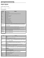
List of Tables
5-1. Front-ends to DLV
5-2. Theory restrictions in abductive diagnostic reasoning
5-3. Theory restrictions in Reiter's diagnostic reasoning
6-1. Front-end Options
6-2. General Options
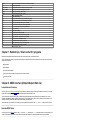
List of Examples
2-1. Simple terms:
2-2. Complex terms:
2-3. Predicates:
2-4. Atoms:
2-5. Literals:
2-6. Facts:
2-7. A program with comments
2-8. Rules:
2-9. Disjunctive facts:
2-10. Constraints:
2-11. Using Anonymous Variables
2-12. True negation vs. negation as failure
2-13. Consistency criterion
2-14. Constraints and negation
2-15.
2-16. Weak Constraints with weights only
2-17. Team Building with weights and priorities
2-18. Comparative predicates:
2-19. Arithmetic predicates:
2-20. List predicates:
2-21. Numeric named constant
2-22. Symbolic named constant
2-23. Assigning a named constant to a named constant
2-24. A weird example program
2-25. Aggregate Predicates
2-26. Symbolic Set Syntax
2-27. Informal meaning of Symbolic Set
2-28. Informal Meaning of Aggregate Functions
2-29. The Cartoons Co. Employees
2-30. #count
2-31. #sum
2-32. #times
2-33. #min
2-34. #max
2-35. Minimum Spanning Tree with Aggregates and Weak Constraints
2-36. The Seating Problem
3-1. Safe Rules and Constraints
3-2. Unsafe Rules and Constraints
3-3. Safe Rules and Constraints
3-4. Unsafe Rules and Constraints
3-5. Not finite domain program
3-6. Not finite domain program
3-7. Finite domain program
3-8. Program generating ever longer lists
3-9. Lists growing both in length and in nesting
4-1. Queries:
4-2. An example for non-ground brave reasoning
4-3. A query with multiple variable occurrences
4-4. A query with negation
4-5. An example for succeeding ground brave reasoning
4-6. Failing ground brave reasoning
4-7. An example for non-ground cautious reasoning
4-8. Succeeding ground cautious reasoning
4-9. Failing ground cautious reasoning
4-10. Succeeding cautious reasoning, if the program does not have any model
4-11. Plain Disjunctive Datalog query
8-1. Simple table import
8-2. Transitive closure on imported table
8-3. Exporting a transitive closure
8-4. Simple import
8-5. 3-coloring with tuple insertion
8-6. 3-coloring with tuple replacement
Overview
DLV is a deductive database system, based on disjunctive logic programming, which offers front-ends to several advanced KR formalisms.
More information (including an online version of this manual) and executables for several platforms are available at the DLV homepage
(http://www.dlvsystem.com/).
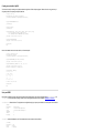
Chapter 1. Getting Started
This is just a quick introduction to Disjunctive Datalog and DLV. For a more thorough and formal definition refer to Chapter 2.
You can invoke DLV directly on the command-line. If you do not specify any options or files, DLV will just print some informational output:
$ DLV
DLV [build BEN/May 23 2004
gcc 2.95.4 20011002 (Debian prerelease)]
usage: DLV {FRONTEND} {OPTIONS} [filename [filename [...]]]
Specify -help for more detailed usage information.
The first line will most probably look different with your installation. It first tells you which program this is, then it gives information about the version. This
consists of the identifier BEN, which stands for "benchmark version",
Note: Versions other than BEN should only be used for development purposes!
the date when the binary was built, and the identifier of the compiler. Usually, you will not have to bother with these gory details, but please include this
information when you are reporting a bug or asking for support.
If you do not want to see this status line, use the -silent option, which suppresses various informational output and blank lines.
$ DLV -silent
usage: DLV {FRONTEND} {OPTIONS} [filename [filename [...]]]
Specify -help for more detailed usage information.
From now on, all examples will include the -silent option.
Since we did not specify any input file, DLV just prints a brief usage message. Let's try with an empty file.
$ DLV -silent empty
{}
The "{}", as noted above, tells you that the input (no program, no database) admits the model in which nothing is true (and as a matter of fact, in which
nothing is false either in this case).
Caution
It is very important to note the difference between an empty model (as above) and no model: If a program has no model, it is contradictory or
inconsistent in some sense, while this is not the case with an empty model.
Chapter 2. The Core Language of DLV: Disjunctive Datalog
DLV's native language is Disjunctive Datalog extended with constraints, true negation and queries.
The most basic elements of Disjunctive Datalog are constants. They refer to entities, just as objects which are stored in relational databases. Constant
names must begin with a lowercase letter and may be composed of letters, underscores and digits. Additionally, all numbers are constants as well.
Note: not is a reserved word and not a valid constant.
Variables are placeholders for constants. Variable names must begin with an uppercase letter and may contain letters, underscores and digits.
There is a special feature, which is called anonymous variable. The anonymous variable is denoted by "_" (the underscore) and is different from a usual
variable as defined in the previous paragraph. Each occurrence of _ represents a new and unique variable, which does not occur anywhere else in the
same rule resp. constraint. Anonymous variables thus can be thought of as preprocessor statements which are substituted by unique variable names
(Actually this description is quite close to what really happens internally). The purpose of this feature is to specify that an argument can be ignored or
does not matter in the current rule resp. constraint without having to invent new and unique variable names.
Note: Since anonymous variables represent unique variables, there is no point of using them in the head of a rule or in a negative literal in
the body, because such rules cannot be safe (see Chapter 3).
A term is either a simple term or a complex term.
A simple term is either a constant or a variable.
Example 2-1. Simple terms:
Constants: a1, 1, 9862, aBc1, c__
Variables: A, V2f, Vi_X3
A complex term is either a funcional term or a list term.
A functional term is a function symbol followed by a parenthesized list of terms. A function symbol must begin with a lowercase letter and may be
composed of letters, underscores and digits.
A list term can have the two following forms:
[t1,... , tn], i.e., a list of terms enclosed in square brackets;
[h|t], where h (the head of the list) is a term, and t (the tail of the list) is a list term ("a la Prolog" syntax).
Note: Since the presence of complex terms could cause the derivation of infinitely many new terms, programs including complex terms are
checked in order to verify if termination is a priori guaranteed (see Chapter 3).
Example 2-2. Complex terms:
Functional terms: f(1), g_1(a), fUN(1,a,f(5)), f(X), f(a,f(gibon(X),1,Y),Zulu)
List terms: [a,[1,2],c,[2,3]], [1,f(1),2,f(a)], [], [1|[2,3]], [a|[b|[c]]], ["Zulu",[],f([])]
Predicates correspond to traditional relations. Predicate symbols begin with a letter and may contain letters, underscores and digits. Again, not is not a
valid predicate.
Example 2-3. Predicates:
ord, oBp, r2D2, E_mc2
An atom is a composition of a predicate symbol and some (possibly none) terms. It is used to represent one or several (by using placeholders) tuples in
the relation identified by the predicate. An atom is denoted by the predicate name, and if there are any terms involved they are written between
parentheses and separated by commata.
The number of terms which a predicate takes in an atom is referred to as arity and must be constant for every predicate.
Example 2-4. Atoms:
a, b(8,K), weight(X,1,kg)
A literal is a (possibly negated) atom. Unlike other systems, DLV supports two types of negation: True (or explicit) negation (as defined by Gelfond and
Lifschitz) and negation-as-failure. True negation is written as - or ~, whereas the negation-as-failure symbol is not.
We refer to an atom which is possibly preceded by a true negation symbol as explicitly negated literal. An explicitly negated literal which is possibly
preceded by the negation-as-failure symbol is simply termed literal.
Example 2-5. Literals:
-a
not ~b(8,K)
not weight(X,1,kg)
Note that an explicit negation symbol followed by the negation-as-failure symbol is not valid syntax.
Facts are explicitly negated literals, which are asserted to be true. Syntactically we denote this by adding a full-stop after the explicitly negated literal.
Note that facts may not contain variables because of the safety criterion (see Chapter 3).
Example 2-6. Facts:
weight(apple,100,gram).
-valid(1,equals,0).
Comments
A DLV program can be documented by adding comments directly to the source. Any line starting with the "%" character, or anything between a "%"
character (that does not occur in a quoted string) and the end of the current line is considered a comment and ignored by DLV.
Example 2-7. A program with comments
% This line is a comment.
weight(apple,100,gram). % Here is a new comment, it ends in this row.
EDB - Extensional Database
Disjunctive Datalog combines databases and logic programming (hence the name!). For this reason, DLV can be seen as a logic programming system
or as a deductive database system. In order to be consistent with deductive database terminology, the input is separated into the extensional database
(EDB), which is a collection of facts, and the intensional database (IDB), which is used to deduce facts.
With DLV, a way to specify such a database is by providing facts in a file, but there is also the possibility to import facts from a relational database,
through ODBC, as described in Chapter 8.
Note: DLV does not require EDB and IDB to be stored in separate files. The same relation may even consist of both EDB and IDB parts.
However, in general it is considered clean if EDB and IDB are separate. To make this separation explicit, we use distinct files for EDB and
IDB in this chapter. The examples also work if the inputs are stored in only one file per example.
The EDB may contain pure propositional knowledge, as in the following example:
hot_furnace.
valve_closed.
Assume that the above (which could be a very simplified description of a steam engine) is stored in a file called engine. Now let us see, what happens if
we call DLV with this input:
$ DLV -silent engine
{hot_furnace, valve_closed}
As expected, the answer contains precisely the two assertions. However, since the EDB is fixed knowledge, displaying it in the output is often not
desired (as it is redundant) or even counterproductive since, for real applications, the EDB will be very large. Using the -nofacts option, predicates
occurring only in the EDB (that is, defined only by means of facts) will not be displayed.
$ DLV -silent -nofacts engine
{}
Unlike in the previous example, the EDB may also contain facts which look like standard relational tuples, rather than propositional atoms:
arc(a,b).
arc(b,c).
arc(b,d).
is called a predicate symbol or relation symbol, the parts within the parentheses are constants. These constants must begin with a lowercase letter
and may contain letters (both upper- and lowercase), underscores and digits. Additionally, all non-negative integer numbers are constants, too.
arc
The EDB above might encode a directed graph which looks like this:
c
^
|
a --> b --> d
Again, since this is an EDB, a call to DLV with the file above (call it simple_graph) results in:
$ DLV -silent simple_graph
{arc(a,b), arc(b,c), arc(b,d)}
and
$ DLV -silent -nofacts simple_graph
{}
IDB - Intensional Database
So far, we have shown how to specify a database serving as input (the EDB). In this section we will show how to define knowledge which can make use
of these input databases.
This knowledge may depend on the EDB, or it may represent independent, but indefinite knowledge, or both. Collectively, this part of the input is termed
intensional database (IDB), or sometimes just program.
Rules state relations between explicitly negated literals. Basically, rules have the following form: h1 v ... v hn :- b1, ..., bm. h1 to hn represent
explicitly negated literals, where n > 0 (i.e. there must be at least one of those). The :- is the transcription of an implication arrow and b1, ..., bm
represent general literals, where m >= 0 must hold (i.e. the body may be omitted completely). The part before the :- is referred to as head, the part after
:- as body. Note that negation-as-failure symbols may occur in the body only. In addition, rules must be safe. For a definition, we refer to Chapter 3.
Informally, if the body evaluates to true, the head must evaluate to true as well. The negation-as-failure symbols can be read as "there is no evidence that
xxx evaluates to true", as in default logic. The head represents a disjunction whereas the body represents a conjunction.
Example 2-8. Rules:
-ok :- not -hazard.
male(X) v female(X) :- person(X).
fruit(P) v vegetable(P) :- plant_food(P).
true v false :- .
employee(P) :- personnel_info(_,P,_,_,_).
Also note that facts can be viewed as special forms of rules, in which the body is empty. The neutral element of conjunction is true, so facts must always
be true. We also allow disjunctive facts as a special case. Note that due to the safety requirement (see Chapter 3), no variables may occur in disjunctive
facts.
Example 2-9. Disjunctive facts:
true v false.
edible(apple) v foul(apple).
The other special form of a rule, in which the head is empty, is called constraint. The neutral element of disjunction is falsity, so the body of a constraint
must not become true, because the head can never become true.
These constructs can be used to constrain the worlds described by the program, hence the name. Since constraints are special forms of rules, they must
meet the safety criterion (see Chapter 3).
Example 2-10. Constraints:
:- color(apple,red), color(apple,green).
:- -healthy(X), not sick(X).
To summarise, a Disjunctive Datalog program consists of an arbitrary number of facts, rules, and constraints.
Definite Rules
The simplest case is if the truth of some statement depends on the truth of some other statements. As an example, reconsider our EDB stored in the file
engine. Let us now define an IDB, which we will store in the file alarm. It should specify that if the furnace is hot (hot_furnace holds) and the pressure
valve is closed (valve_closed holds), then alarm_on should hold.
alarm_on :- hot_furnace, valve_closed.
This construct is called a rule. The :- can be read as "if", and the comma can be considered as an "and". The part to the right of :- is referred to as
body, the left hand side is termed head.
If we call DLV on these two files, we see that alarm_on is indeed derived:
$ DLV -silent engine alarm
{alarm_on}
Note: The ordering of the parameters to DLV does not matter. You can even specify the options at the end or mixed up with the files.
Of course, we usually want to make more general statements, involving some kind of variables. For instance, we might want to define the notion of a path
(i.e., there is a sequence of arcs from one node to a second node) on any graph which is defined by means of the arc predicate. The following IDB does
exactly that:
path(X,Y) :- arc(X,Y).
path(X,Y) :- path(X,Z), arc(Z,Y).
Note that X, Y, and Z are variables. The name of a variable is a sequence of letters, underscores and digits, starting with an uppercase letter. The name
of a predicate can be any sequence of letters, underscores and digits, starting with a lowercase letter.
So the program above says that there is a path from some X to some Y, if there is an arc from X to Y. The second rule is more difficult: It says that a path
exists from X to Y, if there is a path from X to some Z (note that Z did not occur before in this rule) and there is an arc from this Z to Y.
The second rule is worth looking at. The predicate path occurs both in the head and in the body of the rule, so it seems that something is defined by itself
which seems odd. However, this is a common feature in logic programming and is called recursion. You can think of it as assuming that path is already
completely defined, and specifying what conditions have to be met by the defined relation.
Note that variables, which occur in the head, must also occur in the body. This is one of the safety requirements for rules (see Chapter 3).
If we take this program (assume it is stored in a file called path and apply it to the graph defined above, we see:
$ DLV -silent -nofacts simple_graph path
{path(1,2), path(1,3), path(1,4), path(2,3), path(2,4)}
Indeed, this result corresponds to the paths in the graph.
Sometimes a variable is used to mask an argument which is not used in the rest of the rule. For example, if you want to define a node in some graph
(specified in the same format as above), you could write:
node(X) :- arc(X,Y).
node(Y) :- arc(X,Y).
In the first rule Y is used to mask the second argument, in the second rule X masks the first argument of arc.
DLV provides a feature which saves us from the need to invent variable names for these masking variables and which clarifies to readers of programs
that a variable is just used for masking. This feature is called anonymous variable and denoted as _ (an underscore). In spite of its name, an
anonymous variable is not a variable as in the original description. Its meaning can be described as follows: In a preprocessing step, each occurrence of
an anonymous variable is replaced by a unique variable (which does not occur anywhere else in the same rule resp. constraint).
The previous example (defining a node) can thus be rewritten as follows:
Example 2-11. Using Anonymous Variables
node(X) :- arc(X,_).
node(Y) :- arc(_,Y).
Disjunctive Rules
The rules above described definite knowledge, but Disjunctive Datalog (the language we use here) also provides several ways to define indefinite
knowledge.
A simple case is the one, where we know for sure that at least one of two conditions is true, but we are unable to determine which. For example, if we
notice that it is not dark in a room, we know that either the sun shines or that some artificial light is on, or even both:
sunny v light_on.
The v (alternate notions are | and ;) indicates that this construct specifies disjunctive knowledge. Although the above may look similar to a simple fact, it
is no definite knowledge and thus part of the IDB. Now let's see how DLV acts on this input:
$ DLV -silent light
{sunny}
{light_on}
For the first time, the output consists of more than one model. Now it is also clear what a model represents: It represents different worlds for which the
program gives reason. But something seems to miss: What about the model, in which both sunny and light_on are true?
Practically all semantics (definitions of the meaning of a program) have a minimality criterion. That means that if there are two potential models and one
of them is a superset of the other, it should not be considered because it contains some redundant information. Since {sunny, light_on} is a superset
of both {sunny} and {light_on}, it is not considered a proper model.
Note that because of this minimality criterion one disjunctive rule can give reason to exactly one of its atoms in the head. If several head atoms are true in
one rule, there must be some other rules which require the truth of these additional true atoms.
Another example: Say you want to find some node coloring of a graph, which is represented by arcs. That is, we have several colors to choose from, say
red, green, and blue and every node should be assigned one color, but we do not know which one.
To this end, we reuse the node definition of Example 2-11.
The more interesting part is the last rule. Similar to the previous example, we specify that for any node X, either color(X,red), color(X,green) or
color(X,blue) must hold. Here the minimality criterion ensures that exactly one color is assigned to a node.
node(X) :- arc(X,_).
node(Y) :- arc(_,Y).
color(X,red) v color(X,green) v color(X,blue) :- node(X).
Let us view the output by DLV for this example (file coloring) on our example graph in simple_graph:
$ DLV -silent -nofacts coloring simple_graph
{node(1), node(2), node(3), node(4), color(1,red), color(2,red), color(3,red), color(4,red)}
{node(1), node(2), node(3), node(4), color(1,red), color(2,red), color(3,red), color(4,green)}
[... and so on ...]
{node(1), node(2), node(3), node(4), color(1,blue), color(2,blue), color(3,blue), color(4,green)}
{node(1), node(2), node(3), node(4), color(1,blue), color(2,blue), color(3,blue), color(4,blue)}
Negative Rules
We have not yet introduced another important feature of Disjunctive Datalog: negation. Several proposals of what negation should mean in this context
have been made. DLV implements one of those, which has been widely accepted as a reasonable proposal: the Stable Model Semantics.
Negation is treated as "negation as failure". In other words: If an atom is not true in some model, then its negation should be considered to be true in that
model. We will not go into detail here, the examples should give you an idea how this works.
With this mechanism we can, for example, define the complementary graph of a given graph. This is the graph which has the same nodes, but of all
possible arcs, it has exactly those arcs which do not exist in the original graph.
node(X) :- arc(X,_).
node(Y) :- arc(_,Y).
comparc(X,Y) :- node(X), node(Y), not arc(X,Y).
Here comparc describes the set of arcs in the complementary graph. Such an arc must go from one node to another node (possibly the same one), and
this arc must not be contained in the original arc set.
Note that node(X) and node(Y) need to be included in the body in order to satisfy the following safety requirement for rules: Variables, which occur in a
negated literal, must also occur in a positive literal in the body. See Chapter 3.
$ DLV -silent -nofacts simple_graph compl_graph
{node(1), node(2), node(3), node(4), comparc(1,1), comparc(1,3), comparc(1,4), comparc(2,1), comparc(2,2), comparc(3,1), comparc(3,2), comparc(3,3), comparc(3,4), comparc(4,1), comparc(4,2), comparc(4,3), comparc(4,4)}
This was straightforward, but what if negation is used together with recursion? Let us look at a simple example:
bad :- not bad.
Now let us assume a model in which bad is true (in this case {bad}: It is not a valid model, since the only way in which bad could become true is by not
bad being true, which clearly is not the case. On the other hand, a model not containing bad (here {}), is not valid either, because in this case not bad is
true, hence bad must be in the model, but it is not. Consequently, no model exists.
$ DLV -silent bad
So in this case, there is no output at all, because as we have seen, the "empty model" {} is not valid.
Note: Although we did not give any example of this, negation may also occur in the body of disjunctive rules.
True Negation
DLV implements yet another notion of negation: true negation.
Negation as failure, which has been introduced above, does not support explicit assertion of falsity. Rather, if there is no evidence that an atom is true, it
is considered to be false.
There are several situations in which negation as failure is not appropriate because it is necessary that something is explicitly known to be false. For this
reason, true negation is sometimes referred to as explicit negation.
True negation is denoted by preceding an atom with "-" or "~".
Example 2-12. True negation vs. negation as failure
Imagine a simple situation, in which an agent has to cross a railroad. The agent should cross it if there is no train approaching.
With this (sloppy) description, one might specify the following program:
cross_railroad :- not train_approaches.
Since there is no other information, train_approaches does not hold, and cross_railroad is derived:
$ DLV -silent rail_naf
{cross_railroad}
But this is a problem in that the specification should have read "The agent should cross, if it is explicitly known that no train approaches". The difference
is how incomplete information is handled. In the first case, information, whose truth value is unknown, may be used for inference, in the second case this
is forbidden. So we utilise true negation:
cross_railroad :- -train_approaches.
In this case, -train_approaches can be considered as a separate atom, and since there is no information that it holds, cross_railroad cannot be
derived.
$ DLV -silent rail_true
{}
Example 2-13. Consistency criterion
An atom and its explicitly negated counterpart may never occur in the same model. In the literature, "models" of programs containing true negation are
called "answer sets". If atoms a and -a occur in the same answer set, it is inconsistent. An inconsistent answer set contains all (possibly explicitly
negated) literals of the language. In our framework, inconsistent models do not exist.
a.
-a.
This program has no model.
Integrity Constraints
Constraints in our framework specify conditions which must not become true in any model. In other words, constraints are formulations of possible
inconsistencies. This mechanism is very useful in connection with disjunctive rules. The disjunctive rules serve as generators for different models and the
constraints are used to select only the desired ones.
The syntax of constraints is simple: They look like rules without heads. As with rules, constraints must meet the safety requirements (see Chapter 3).
A very well-known problem is to find a coloring of a graph, such that no two adjacent nodes (i.e. two nodes which are connected by an arc) have the
same color.
To formulate this problem in Disjunctive Datalog, let us reconsider the coloring example from above:
node(X) :- arc(X,_).
node(Y) :- arc(_,Y).
color(X,red) v color(X,green) v color(X,blue) :- node(X).
The models of this program (together with a database describing the graph) correspond to all possible colorings. We only need to add a constraint
which discards colorings where two adjacent nodes have the same color:
:- arc(X,Y), color(X,C), color(Y,C).
Assuming the combined code resides in 3col, the output then is:
$ DLV -silent -nofacts simple_graph 3col
{node(1), node(2), node(3), node(4), color(1,red), color(2,green), color(3,red), color(4,red)}
[... and so on ...]
{node(1), node(2), node(3), node(4), color(1,blue), color(2,green), color(3,blue), color(4,red)}
{node(1), node(2), node(3), node(4), color(1,blue), color(2,green), color(3,blue), color(4,blue)}
Note that this program yields 24 models, while the previous coloring example led to 81 models.
Example 2-14. Constraints and negation
Of course, also negation can be used in constraints:
a v b.
:- not a.
{a}
is a model of this program, but {b} is not, since the constraint would be violated for {b}.
As a comparison, a constraint with true negation:
a v b.
:- -a.
Both {a} and {b} are models, since -a is not contained in any of these models.
Weak Constraints
This feature allows us to formulate several optimization problems in an easy and natural way. While standard constraints (integrity constraints, strong
constraints) always have to be satisfied, weak constraints express desiderata, i.e., they should be satisfied if it is possible, but their violation does not
"kill" the models.
The answer sets of a program P with a set W of weak constraints are those answer sets of P which minimize the number of violated weak constraints.
They are called Best Models of (P,W). Note that a program may have several best models (violating the same number of weak constraints).
Weak constraints can be weighted according to their importance (the higher the weight, the more important the constraint). In the presence of weights,
best models minimize the sum of the weights of the violated weak constraints. Weak constraints can also be prioritized. Under prioritization, the
semantics minimizes the violation of the constraints of the highest priority level first; then the lower priority levels are considered one after the other in
descending order.
Syntactically, weak constraints are specified as follows.
:~ Conj. [Weight:Level]
where Conj is a conjunction of (possibly negated) literals, and both Weight and Level are positive integers.
Weights and priority levels are allowed to be variables, provided that these variables also appear in a positive literal in Conj. The user can omit the
weight or the priority or both, but all weak constraints must have the same syntactic form (i.e., the user is free to specify only weights or only priorities, or
both, but all constraints of the program must have the same syntactic form).
Example 2-15.
Consider the following program stored in a file called example1.
a v b.
c :- b.
:~ a.
:~ b.
:~ c.
Since weights and priority levels are omitted, their values are set to 1 by default. If we feed this program into DLV, we obtain the following output:
$ DLV -silent example1
Best Model: {a}
Cost ([Weight:Level]): <[1:1]>
Note that the answer sets of { a v b. c :- b. } are {a} and {b, c}. The presence of weak constraints discards {b, c} because it violates two weak
constraints (while {a} violates only one weak constraint).
Example 2-16. Weak Constraints with weights only
The following program, stored in a file called min_sp, computes the minimum spanning trees of a weighed directed graph.
root(a).
node(a). node(b). node(c). node(d). node(e).
edge(a,b,4). edge(a,c,3). edge(c,b,2). edge(c,d,3). edge(b,e,4). edge(d,e,5).
in_tree(X,Y,C) v out_tree(X,Y) :- edge(X,Y,C), reached(X).
:- root(X), in_tree(_,X,C).
:- in_tree(X,Y,C), in_tree(Z,Y,C), X != Z.
reached(X):- root(X).
reached(Y):- reached(X), in_tree(X,Y,C).
:- node(X), not reached(X).
:~ in_tree(X,Y,C). [C:1]
The output of this program is
$ DLV -silent -nofacts min_sp_tree
Best model: {reached(a), out_tree(a,b), in_tree(a,c,3), reached(b), reached(c),
in_tree(b,e,4), in_tree(c,b,2), in_tree(c,d,3), reached(e), reached(d),
out_tree(d,e)}
Cost ([Weight:Level]): <[12:1]>
Finally, we show an example where both weights and priorities are specified.
Example 2-17. Team Building with weights and priorities
Consider the problem of assigning a given set of employees to two projects. As a minor desideratum, we wish that members of the same group already
know each other.
Higher level constraints ask each group to be heterogeneous as far as skills are concerned, and require that people married with one another do not
work in the same group. We can define the following program in file called plan.
employee(a). employee(b). employee(c). employee(d). employee(e).
know(a,b). know(b,c). know(c,d). know(d,e).
same_skill(a,b).
married(c,d).
member(X,p1) v member(X,p2) ::~ member(X,P), member(Y,P), X
:~ member(X,P), member(Y,P), X
:~ member(X,P), member(Y,P), X
employee(X).
!= Y, not know(X,Y). [1:1]
!= Y, married(X,Y). [1:2]
!= Y, same_skill(X,Y). [1:2]
This program has two best models:
$ DLV plan -silent -filter=member
Best
Cost
Best
Cost
model: {member(a,p2), member(b,p1), member(c,p1), member(d,p2), member(e,p2)}
([Weight:Level]): <[6:1],[0:2]>
model: {member(a,p1), member(b,p2), member(c,p2), member(d,p1), member(e,p1)}
([Weight:Level]): <[6:1],[0:2]>
If you specify the -costbound=weight[,weight] option on the command line, all of the models with a cost less-or-equal than costbound will be computed.
Note that not all of the computed models will be best models. You can associate a positive integer with each priority level of costbound. If, instead of an
integer, _ is specified the corresponding weight is unbound. For instance, running DLV with the option
$ DLV take2.dl -costbound=5,10,_
sets up an upper bound for the cost of the computed models, where the first two priority levels must have a value less-or-equal than 5 and 10,
respectively, while the last one is unbound. Note that the rightmost weight is associated with the highest level. If you specify fewer priority levels than
occur in the input, only weights corresponding to the lower priorities will set up the upper bound of the cost, the remaining levels will be unbound. On the
other hand, superfluous higher levels will be ignored.
For instance, running the following command line for Example 2-16 we will obtain the following results
$ DLV min_sp_tree -silent -filter=member -costbound=13
{in_tree(a,c), in_tree(c,b), in_tree(c,d), in_tree(d,e)}
Cost ([Weight:Level]): <[13:1]>
{in_tree(a,c), in_tree(b,e), in_tree(c,b), in_tree(c,d)}
Cost ([Weight:Level]): <[12:1]>
If costbound is less than the cost of the best model(s), no model is output.
Note that the number of computed models can be limited also under option -costbound. For instance running
$ DLV take2.dl -costbound=10 -n=1
asks for computing one model whose cost is at most 10.
Note: In presence of weak constraints adding the option -n=1 may speed up the computation significantly in some cases. Also the
specification of a costbound may improve the efficiency.
specification of a costbound may improve the efficiency.
Built-in predicates
In addition to those predicates defined by the user, some predicates are already built into DLV and available for all programs. These predicates have
names different from those that can be defined by users and must not be redefined. An atom with a built-in predicate is referred to as a built-in atom.
Like ordinary atoms, built-in atoms can be negated by using negation-as-failure.
Comparative Predicates
Constants can be compared by means of the built-in predicates
<, >, <=, >=, = (with == as a deprecated alternative), !=
writable in normal prefix or infix notation. All kinds of constants (symbols and integers) may be compared against each other freely. If two integers are
compared, the semantics are as expected. All other comparisons are just guaranteed to impose a fixed ordering over all constants.
Example 2-18. Comparative predicates:
in_range(X,A,B) :- X>=A, <(X,B).
pair(X,Y) :- Y>X, color(X,green), color(Y,green).
In the second example, pair is guaranteed to define an asymmetric relation. I.e., if pair(A,B) holds, pair(B,A) does not. As a direct consequence, no A
exists, such that pair(A,A) holds.
All variables occurring in comparative predicates are required to satisfy a safety condition as reported in Chapter 3.
Arithmetic Predicates
Reasoning and computing over a finite set of integer ranges is possible with the predicates
#int, #succ, #prec, #mod, #absdiff, #rand, +, *, -, /
The unary version of the #int builtin is only defined if an upper integer limit N is given on the command-line (with -N=N - see Chapter 6). Note that, such
option limits the integers known by DLV to the range [0,N] and no arithmetic predicate will generate integers outside of the known range. If integer
constants outside this range occur in the input, an error is issued.
is true, iff X<=Z<=Y holds.
is true, iff X is a known integer (i.e. 0<=X<=N).
#succ(X, Y) is true, iff X+1=Y holds.
#prec(X, Y) is true, iff X-1=Y holds.
#mod(X, Y, Z) is true, iff X%Y=Z holds.
#absdiff(X, Y, Z) is true, iff abs(X-Y)=Z holds.
#rand(X, Y, Z) is true, iff Z is a randomly generated integer such that X<=Z<=Y holds.
#rand(X) is true, iff X is a randomly generated integer such that X>=0 and X is not greater than the maximum value for integers.
+(X,Y,Z), or alternatively: Z=X+Y is true, iff Z=X+Y holds.
*(X,Y,Z), or alternatively: Z=X*Y is true, iff Z=X*Y holds.
-(X,Y,Z), or alternatively: Z=X-Y is true, iff Z=X-Y holds.
/(X,Y,Z), or alternatively: Z=X/Y is true, iff Z=X/Y holds.
#int(X, Y, Z)
#int(X)
Each arithmetic built-in has a number of input arguments and exactly one output argument. The output argument is always the last one and its value is
computed from the values of input arguments.
Input arguments are required to satisfy a safety condition as specified in Chapter 3.
Example 2-19. Arithmetic predicates:
fibonacci(N,F) :- #succ(N2,N1), #succ(N1,N), fibonacci(N1,F1), fibonacci(N2,F2), +(F1,F2,F).
previousSec(Y) :- sec(X), #prec(X,Y).
even(X) :- #int(X), #mod(X,2,0).
odd(X) :- #int(X), not #mod(X,2,0).
weight(X,KG,kilogram) :- weight(X,G,gram), *(G,1000,KG).
product(X) :- #int(P), #int(Q), X=P*Q.
productOfPrimes(X) :- #int(P), #int(Q), X=P*Q, P>1, Q>1.
prime(A) :- #int(A), not productOfPrimes(A).
netWeight(X,N) :- fullweight(X,W), tare(X,T), N=W-T.
monthlyFee(Y) :- fee(X), Y=X/12.
sameDiagonal(X1,Y1,X2,Y2) :- cell(X1,Y1), cell(X2,Y2), X1!=X2, Y1!=Y2, #absdiff(X1,X2,D), #absdiff(Y1,Y2,D).
diceRoll(X) :- #rand(1,6,X).
The following small example file
number(X) :- #int(X).
demonstrates the range of valid integers. It results in output like this:
$ DLV -silent -N=5 number
{number(0), number(1), number(2), number(3), number(4), number(5)}
This example shows a use of #succ:
lessthan(A,B) :- #int(A), #succ(A,B).
lessthan(A,C) :- lessthan(A,B), #succ(B,C).
The output is as follows:
$ DLV -silent -N=3 lessthan
{lessthan(0,1), lessthan(0,2), lessthan(0,3), lessthan(1,2),
lessthan(1,3), lessthan(2,3)}
List Predicates
A number of predicates are available for reasoning and computing over list terms:
#append, #delnth, #flatten, #getnth, #head, #insLast, #insnth, #last, #length, #member, #reverse, #subList, #tail
All list built-ins (except #member and #subList) have a number of input arguments and exactly one output argument. The output argument is always the
last one and its value is computed from the input arguments. It must be either a variable or a constant term, i.e. it cannot be a complex term that is not
constant. Built-ins #member and #subList do not produce any output but just perform a check on their input arguments.
#append(X, Y, Z)
#delnth(X, Y, Z)
valid position in X.
is true iff Z is a list obtained by appending the elements of Y to X. X and Y must be list terms.
is true iff Z is a list obtained from deleting the element of X at position Y. X must be a list term and Y must be a number referring to a
is true iff Y is a list obtained from flattening X. X must be a list term.
is true iff Z is the element at position Y in the list X. X must be a list term and Y must be a number referring to a valid position in X.
#head(X, Y) is true iff Y is the first element of X. X must be a list term.
#insLast(X, Y, Z) is true iff Z is a list obtained by appending the term Y to X. X must be a list term, Y can be any term.
#insnth(X, Y, Z, W) is true iff W is a list obtained by inserting the term Y into X at position Z. X must be a list term, Y can be any term and Z must be a
number referring to a valid position in X.
#last(X, Y) is true iff Y is the last element of X. X must be a list term.
#length(X, Y) is true iff Y is the size of X. X must be a list term.
#member(X, Y) is true iff X is a member of Y. X can be any term whereas Y must be a list term.
#reverse(X, Y) is true iff Y is a list obtained from reversing X. X must be a list term.
#subList(X, Y) is true iff X is a sublist of Y. X and Y must be list terms.
#tail(X, Y) is true iff Y is the list containing all elements but the first of X. X must be a list term.
#flatten(X, Y)
#getnth(X, Y, Z)
List built-ins #append, #insLast and #insnth may cause the evaluation of a program to not terminate because they could generate ever longer lists. See
section Chapter 3 for further information.
Example 2-20. List predicates:
newList(X) :- #append([a,b,c],[d,e],X).
newList(X) :- #delnth([a,b,c],1,X).
flattenedList(X) :- #flatten([a,b,[c,[d]]],X).
anElement(X) :- #getnth([a,b,c],2,X).
headElement(X) :- #head([a,b,c],X).
newList(X) :- #insLast([a,b,c],d,X).
newList(X) :- #insnth([a,b,c],d,4,X).
lastElement(X) :- #last([a,b,c],X).
size(X) :- #length([a,b,c],X).
yes :- #member(c,[a,b,c]).
reversedList(X) :- #reverse([a,b,c],X).
yes :- #subList([c],[a,b,c]).
tailList(X) :- #tail([a,b,c],X).
Facts over a fixed Integer Range
As a shortcut for defining unary facts ranging over a sequence of integer values you can use the following syntax:
pred(X..Y).
where pred is a predicate name and X,Y are integers less or equal to the upper integer limit (as given on the command-line with -N - see Chapter 6) and
X should be less or equal than Y (in order to produce any results).
For example:
weekday(1..7).
is equivalent to adding the facts
weekday(1).
weekday(2).
weekday(3).
weekday(4).
weekday(5).
weekday(6).
weekday(7).
Built-in constants
equals the upper integer limit (as given on the command-line with -N - see Chapter 6). Using #maxint if there was no integer range defined
results in an error.
#maxint
In addition to the command-line option -N, #maxint can also be set directly in the input, as in the following example.
#maxint=19.
bignumber(#maxint).
Named constants
A name can be assigned to a constant. This can be useful when the same constant is used many times in your program and you want to change its
value.
To define a new named constant use the following syntax:
#const namedConstant = constant.
where namedConstant is a constant name (it must begin with a lowercase letter and may be composed of letters, underscores and digits) and constant
is any legal constant term. Following such a definition, all occurrences of namedConstant are replaced with constant. The definition of a new value for an
already defined named constant is not allowed.
Example 2-21. Numeric named constant
#const rate = 5.
due(2). due(10).
pay(X) :- due(Y), X=Y*rate.
The output is as follows:
$ DLV -silent -N=50 numconst
{due(2), due(10), pay(10), pay(50)}
Example 2-22. Symbolic named constant
#const nickname = mickey.
username(u1). username(u2).
user(X,nickname) :- username(X).
The output is as follows:
$ DLV -silent symconst
{username(u1), username(u2), user(u1,mickey), user(u2,mickey)}
Note that a named constant appearing on the right side of a named constant definition will be treated like a regular constant.
Example 2-23. Assigning a named constant to a named constant
This example should clarify the previous note.
#const rate = 5.
#const new_rate = rate.
p(rate).
p(new_rate).
The output is as follows:
$ DLV -silent remark1
{p(5), p(rate)}
It is explicitly forbidden to define a named constant, which has already been used as a regular constant.
Example 2-24. A weird example program
#const a = b.
#const b = a.
a(a).
b(b).
The output is as follows:
$ DLV -silent remark2
line 2: constant term 'b' already used.
Aborting due to parser errors.
Aggregate Predicates
Aggregate predicates allow to express properties over a set of elements. They can occur in the bodies of rules and constraints, possibly negated using
negation-as-failure. DLV programs with aggregates often allow clean and concise problem encodings by minimizing the use of auxiliary predicates and
recursive programs, and help the DLV programmer to depict problems in a more natural way. From the point of efficiency, encodings using aggregates
often outperform those without, since the size of the ground instantiation tends to be much smaller in this case.
Example 2-25. Aggregate Predicates
q :- 0 <= #count{X,Y : a(X,Z,k),b(1,Z,Y)} <= 3.
q(Z) :- 2 < #sum{V : d(V,Z)}, c(Z).
p(W) :- #min{S : c(S)} = W.
:- #max{V : d(V,Z)} > G, c(G).
Using the example above we introduce the main features of the aggregate predicates:
The sets appearing in curly braces are called Symbolic Sets.
#count, #sum, #times, #min, and #max
are called aggregate functions, and DLV currently supports exactly these five. An aggregate function is applied
over a set and returns a numeric value.
The terms 0, 2, 3, G, W are called guards.
Guards can be numbers or variables. They provide a range to compare the value returned by the aggregate function. If the value is in the range then the
aggregate predicate is true, it is false otherwise. Moreover an aggregate predicate is false if a guard is a variable instantiated with a non numerical
value.
The term W above is an assignment guard which assigns the value returned by the aggregate function to a variable. If the guard is an assignment, the
aggregate is always true.
In the next sections we provide details on syntax and informal meaning of the aggregate predicates features. Moreover we show several examples of
program encodings, and finally we present two problems from AI encoded with aggregates.
Symbolic Sets
The syntax of a Symbolic Set is
{Vars : Conj}
where Vars is a list of local variables (see below), and Conj is a conjunction of (non-aggregate) literals.
The following is an example of a symbolic set occurring in an aggregate.
Example 2-26. Symbolic Set Syntax
q(Z) :- 1 < #count{X : a(X,Y,Z), not d(2,Y,goofie)}, c(Z).
Variable X is local, i.e. it occurs in at least one literal of Conj, and does not appear anywhere outside of the symbolic set (note that it can not occur in any
other symbolic set defined in the same rule). Literals of Conj can contain constants, local variables, and global variables (i.e. variables also appearing
outside the symbolic set). In the example Example 2-26 Vars consists of the local variable X. Y is also a local variable, while Z is a global variable.
Finally, 2 and goofie are constants. We will further discuss safety of variables occurring in a symbolic set in Chapter 3.
Example 2-27. Informal meaning of Symbolic Set
Consider the following symbolic set
{V : d(V,3)}
The ground instantiation of this symbolic set consists of pairs V,d(V,3) such that d(V,3) is true w.r.t. the current interpretation.
Given an interpretation
I = {d(1,1), d(1,3), d(3,3)}
the true instances of d(V,3) w.r.t. I are
d(1,3)
d(3,3)
hence the symbolic set is given by
S = {<1,d(1,3)>, <3,d(3,3)>}
Aggregate Functions
An aggregate function applies to the symbolic set, and returns a number.
Example 2-28. Informal Meaning of Aggregate Functions
The aggregate function #count returns the cardinality of the symbolic set to which is applied. If we apply #count to the symbolic set from example
Example 2-27 w.r.t. interpretation I.
Example 2-27 w.r.t. interpretation I.
#count{<1,d(1,3)>, <3,d(3,3)>}
the returned value is 2.
In the following we show syntax and informal meaning of all the aggregate functions supported by DLV by examples. In order to do that, we introduce the
following EDB representing the employees of a company.
Example 2-29. The Cartoons Co. Employees
Each employee is is represented by a fact of the form emp(ID,NAME,SALARY) which we store in a file called employees.
emp(1,goofie,1250).
emp(2,willy,700).
emp(3,woody,750).
emp(4,jerry,900).
emp(5,tom,1050).
Example 2-30. #count
Aggregate function #count returns the cardinality of the symbolic set to which it is applied.
We want to count how many employees of the company earn more than 1000. The program is stored in a file called query1.dl.
over1000(I,S) :- emp(I,N,S), S > 1000.
over1000nr(X) :- #count{I : over1000(I,W)} = X.
Intuitively the symbolic set appearing in the aggregate predicate consists of two ground predicates
{<1,over1000(1,1250)>,<5,over1000(5,1050)>}
which are both true w.r.t. the unique model of the whole program, hence
#count{over1000(1,1250),over1000(5,1050)}
returns 2, and the output is
$ DLV -silent -nofacts employees query1.dl
{over1000(1,1250), over1000(5,1050), over1000nr(2)}
Note: Please note that we can also rewrite the program omitting the first rule and changing the second one as follows:
over1000nr(X) :- #count{I : emp(I,N,S),S>1000} = X.
To check whether there is any employee earning more than 1200, we can write the following program stored in a file named query2.dl
warnMeOver1200 :- #count{I : emp(I,N,S), S > 1200} > 0.
Example 2-31. #sum
#sum returns the sum of the first local variable to be aggregated over in the symbolic set.
Suppose we want to know how much Cartoon Co. spends on salaries. This can be easily implemented using the following program query3.dl.
salaryTotal(X) :- #sum{S,I : emp(I,N,S)} = X.
The symbolic set here consists of 5 elements, namely all of the facts stored in the database of the employees. The aggregate function applied to the
given set returns the sum of the salaries of all the employees, the output thus is:
$ DLV -silent -nofacts employees query3.dl
{salaryTotal(4650)}
Note: The sum is formed only over S, the first variable in the set, while the specification of I is necessary to guarantee that one value per
employee is summed. If only S was specified, then if two distinct employees earn the same amount of value, this amount would be summed
only once instead of twice.
If we look only at the projection on S, then specifying S represents the set of values for S, for which emp(I,N,S) holds, while specifying S,I
represents the multiset of values for S, for which emp(I,N,S) holds.
To check whether the expenses for salaries exceed 4500, we can use the following simple program:
warning :- #sum{S,I : emp(I,N,S)} > 4500.
Example 2-32. #times
#times is similar to #sum, but computes the product of the first local variable to be aggregated over in the symbolic set. When applied over the empty
set, #times returns 1.
Example 2-33. #min
#min returns the minimum value of the first local variable to be aggregated over in the symbolic set.
The following simple program then returns the lowest income among all employees.
lowest(X) :- #min{S : emp(I,N,S)} = X.
To perform the same query without aggregate predicates we would need to write the following program consisting of the query plus an auxiliary rule
which is by far less elegant.
lowest(X) :- emp(_,_,X), not existsLowerThan(X).
existsLowerThan(W) :- emp(_,_,W), emp(_,_,W1), W1 < W.
Example 2-34. #max
#max returns the maximum value of the first local variable to be aggregated over in the symbolic set.
The following program computes the maximum income earned in the company
highest(X) :- #max{S : emp(I,N,S)} = X.
Running this program with DLV generates the following output:
$ DLV -nofacts employees query6.dl
{highest(1250)}
Knowledge Representation Using Aggregate Predicates
In the following we present several examples of well-known problems in the field of Artificial Intelligence which can be represented in a very elegant and
readable way by means of aggregates.
Example 2-35. Minimum Spanning Tree with Aggregates and Weak Constraints
The following program is an alternate version of the program Example 2-16, where integrity constraints are rewritten by using aggregates.
The strong constraint
:- root(X), in_tree(_,X,C).
ensuring that "the root of a tree should not have any incoming arc" can be rewritten as follows
:- root(R), not #count{X : in_tree(X,R,C)} = 0.
The constraint
:- in_tree(X,Y,C), in_tree(Z,Y,C), X != Z.
ensuring that "each node in the tree must have only one incoming arc" can be rewritten as
:- edge(_,Y,_), not #count{X : in_tree(X,Y,_)} = 1.
Please note that the previous definition ensures also that "each node in the graph should be reached (i.e. must belong to the spanning tree)", hence in
this version of the program the following part
reached(X) :- root(X).
reached(Y) :- reached(X), in_tree(X,Y).
:- node(X), not reached(X).
is redundant, and can be omitted. Thus the rewritten IDB of the program appears as follows
in_tree(X,Y,C) v out_tree(X,Y) :- edge(X,Y,C).
:- root(R), not #count{X : in_tree(X,R,C)} = 0.
:- edge(_,Y,_), not #count{X : in_tree(X,Y,_)} = 1.
:~ in_tree(X,Y,C). [C:1]
Comparing this encoding with the one from Example 2-16, we obtain improved readability (aggregates are more meaningful also to entry-level users)
and more elegant definitions (without auxiliary rules.).
Example 2-36. The Seating Problem
Assume we store facts specifying a set of 24 persons and facts defining whether couples of people like or dislike each other in a file called rel:
npersons(24). % number of people
#maxint = 24. % number of people
person(K1):- #int(K1), K1 > 0, K1 <= K, npersons(K).
like(1,2).
dislike(2,3).
...
Furthermore, assume we have another file called restaurant which specifies the number of tables and the number of seats for each table of a
restaurant:
ntables(3).
nchairs(8).
% number of tables
% number of chairs
Consider the problem of assigning seats to the set of people. Each person should be assigned to a seat S of a table T, where she she will meet only
people she likes and nobody she dislikes. We can encode this problem by means of aggregates.
% Guess if person P sits at table T or not.
at(P,T) v not_at(P,T) :- person(P), table(T).
% The number of persons at a table T must not exceed the number of chairs.
:- table(T), nchairs(C), not #count { P: at(P,T) } <= C.
% A person is seated at precisely one table.
:- person(P), not #count{T : at(P,T)} = 1.
% People who like each other should sit at the same table.
:- like(P1,P2), at(P1,T), not at(P2,T).
% People who dislike each other must not sit at the same table.
:- dislike(P1,P2), at(P1,T), at(P2,T).
Chapter 3. Safety
DLV imposes a safety condition on variables in rules. This guarantees that a rule is logically equivalent to the set of its Herbrand instances.
Standard, Arithmetic and Comparative Predicates
A variable X in an aggregate-free rule is safe if at least one of the following conditions is satisfied:
X
occurs in a positive standard predicate in the body of the rule;
X
occurs in a true negated standard predicate in the body of the rule;
X
occurs in the last argument of an arithmetic predicate A and all other arguments of A are safe.
A rule is safe if all its variables are safe. However, cyclic dependencies are disallowed, e.g., :- #succ(X,Y), #succ(Y,X) is not safe.
Example 3-1. Safe Rules and Constraints
a(X) :- not b(X), c(X).
a(X) :- X > Y, node(X), node(Y).
a(Y) :- number(X), #prec(X,Y).
a(Z) :- number(X), #succ(X,Y), Z=X+Y.
:- number(X), number(Y), #mod(X,Y,2).
:- -a(Y), not b(Y), not c(Y).
Example 3-2. Unsafe Rules and Constraints
a(X) v -a(X).
a(X) :- not b(X).
a(X) :- number(Y), X=Y*Z.
a(X) :- number(Y), #succ(X,Y).
:- not number(X), #succ(X,Y).
:- not -b(Y).
:- X <= Y, node(X).
Aggregates
A variable X appearing in the symbolic set of an aggregate is safe if it does not appear elsewhere outside the aggregate atom and at least one of the
following conditions is satisfied:
X
occurs in a positive standard predicate in the symbolic set;
X
occurs in a true negated standard predicate in the symbolic set;
X
occurs in the last argument of an arithmetic predicate A in the symbolic set and all other arguments of A are safe.
All other variables (including guards) appearing in an aggregate atom have to be made safe by some other literal of the body.
Example 3-3. Safe Rules and Constraints
a(X) :- node(X), #count{V : edge(V,X)} >0.
a(X) :- node(X), not #count{V : edge(V,X)} =0.
a(X) :- #count{V : node(V), #succ(V,Z), not node(Z)} =X.
:- #count{V : edge(V,Y), not edge(Y,V)} =X, X>2.
:- not node(X), #count{V : edge(V,Y)} =X.
Example 3-4. Unsafe Rules and Constraints
a(X) :- not node(X), #count{V : edge(V,X)} > 0.
a(X) :- node(X), #count{V : edge(V,X)} >Z.
a(X) :- node(X), #count{V : edge(V,X), not edge(V,Y)} > 0.
a(X) :- #count{V : node(V), not edge(V,Y), Y=V+Z} > 0.
:- #count{V : edge(V,Y), not edge(Y,X)} >0, X>2.
:- #count{V : edge(V,Y)} >0, X>Y.
:- not node(X), #count{V : edge(V,Y)} >X.
An assignment aggregate aggregateFunction{symbolicSet} =X makes X safe. However, as for arithmetic predicates, cyclic dependencies are
disallowed. For instance, the following rule is unsafe because of a cyclic dependency between two aggregates:
a(Z) :- #count{V : edge(V,Z)} =X, #count{T : edge(T,X)} =Z.
The following rule is unsafe because of a cyclic dependency between a built-in and an aggregate:
a(Z) :- node(X), #count{V : edge(V,Z)} =Y, Z=X+Y.
Finite Domain Check
In case of programs with arithmetic predicates or complex terms, a finite domain check is performed in order to verify if termination is guaranteed. This
check is enabled by default, but can be disabled/enabled by using proper options (-nofinitecheck/-finitecheck see Chapter 6).
Arithmetic Predicates
By evaluating a program with arithmetic predicates it is possible to derive new numeric constants, different from those already occurring in the program.
In case of recursive rules, this could cause the non-termination of the evaluation so an error message is issued in this case.
Example 3-5. Not finite domain program
p(0).
p(Y) :- p(X), #succ(X,Y).
To safely evaluate this kind of programs an upper integer limit N has to be specified either on the command-line (with -N=N - see Chapter 6) or in the
program (with #maxint=N.).
Complex Terms
Evaluation of a program might not terminate if a complex term occurs in the head of a recursive rule.
Example 3-6. Not finite domain program
p(0).
p(f(X)) :- q(X).
q(X) :- p(X).
Some programs can be safely evaluated even if there are complex terms appearing in the head of a rule. This is the case when all arguments of a
functional term are restricted to range over a finite domain thanks to the presence of some other atoms in the body.
Example 3-7. Finite domain program
p(0). r(0).
p(f(X)) :- r(X), q(X).
q(X) :- p(X).
When a program is not recognized to have a finite domain and termination thus cannot be guaranteed, an error is issued. The program can be evaluated
in any case, skipping the finite domain check by using the -nofinitecheck command-line option. The -maxnesting=N command-line option can be used
in order to limit the maximum nesting level for complex terms to N (see Chapter 6).
In the presence of list terms, program evaluation may not terminate for two different reasons. The first is an indefinite increase of nesting levels for newly
generated lists, similar to functional terms. The second reason is the indefinite increase in length of lists. The following example shows a program whose
evaluation does not terminate because of the generation of ever longer lists.
Example 3-8. Program generating ever longer lists
p([]). q(0).
p([X|Y]) :- q(X), p(Y).
The -maxlist=N command-line option can be used in order to limit to N the maximum length for list terms (see Chapter 6). Note that a program with lists
may need to have both options set because -maxnesting limits growth in nesting whereas -maxlist limits growth in length.
Example 3-9. Lists growing both in length and in nesting
p([]). p(0).
p([X|Y]) :- p(X), p(Y).
Chapter 4. Queries
In general, by posing a query one looks for ground substitutions such that the substitution applied to the query is true or validated by the rest of the
program. Since a Disjunctive Datalog program may have more than one model, there are different reasoning modes resp. front-ends (brave [cf. the
Section called Brave Reasoning] and cautious [cf. the Section called Cautious Reasoning]) to decide whether a substituted query is satisfied.
The query syntax is the same for all types of queries described in the previous paragraph: Queries consist of one or more literals, which must be
separated by commata and terminated by a question mark. Only one query per program is considered.
Note: If you specify more than one query, only the last one will be considered and DLV will issue an appropriate message.
A special case arises when the query is ground. In this case, there is only one meaningful substitution to consider (the empty substitution), and therefore
the task of finding a substitution boils down to a decision of whether the empty substitution is admissible or not. For brave reasoning [cf. the Section
called Brave Reasoning] this means deciding whether there exists an answer set in which the query holds, and for cautious reasoning [cf. the Section
called Cautious Reasoning] the task is deciding whether the query holds in all answer sets. For ground queries, there is a third alternative: One might be
interested in which models the query is satisfied (cf. the Section called Plain Disjunctive Datalog).
Example 4-1. Queries:
The following three are ground queries,
not a ?
a, -b ?
not ~a2(h,i,j,k), not b1(1,2,3) ?
while the next three are non-ground queries.
a(X) ?
a(Y), -b(Y) ?
not ~a2(Z,i,X,k), b1(X,Z,3) ?
Note: Note that the conjunction in a query must be safe, just like a rule body, as described in Chapter 3.
Brave Reasoning
If you specify -brave on the command line, brave (or credulous) reasoning is selected. In this mode, a query must be specified. A query is bravely true
for a substitution, if its conjunction, on which the substitution has been applied, is satisfied in at least one model of the program.
DLV will output all substitions for which the wuery is bravely true. Each substitution is listed on a separate line, in the form of a list of constants. When
ordering the variables of the query by their first occurrence, this list specifies the corresponding constants substituted for the variables. When no model
exists, DLV will output No stable model found. instead of nothing.
Example 4-2. An example for non-ground brave reasoning
Consider a simple three-coloring example. We have three input files, one with map data (map):
borders(technocratia,absurdistan).
borders(technocratia,schilda).
borders(technocratia,shangri_la).
borders(schilda,absurdistan).
borders(schilda,shangri_la).
A second file contains the program and a pre-coloring information that shangri_la should be colored blue (file coloring):
country(C) :- borders(C,_).
country(C) :- borders(_,C).
colored(C,red) v colored(C,blue) v colored(C,yellow) :- country(C).
colored(shangri_la,blue).
:- colored(C1,Col), colored(C2,Col), borders(C1,C2).
A third file (coloring.query.1) contains our query, which (under brave reasoning) just asks for colorings that are possible in any scenario:
colored(C,Col)?
Let us now call DLV on these files with the brave reasoning front-end:
$ DLV -silent -brave map coloring coloring.query.1
shangri_la, blue
technocratia, red
technocratia, yellow
absurdistan, blue
schilda, red
schilda, yellow
Note: The -silent flag is only used to suppress some version information and similar output.
Note: Each line corresponds to a substitution, in which the first constant is the substitute for C and the second constant is the substitute for
Col.
Example 4-3. A query with multiple variable occurrences
Let us consider the setting of Example 4-2 and specify a different query in file coloring.query.2), asking for the color assigned to schilda and the
countries that have been assigned this color in some scenario:
colored(schilda,Col), colored(C,Col)?
We get:
$ DLV -silent -brave map coloring coloring.query.2
red, schilda
yellow, schilda
Note: Here, the first constant is the substitute for Col and the second constant is the substitute for C, because Col occurs before C in the
query of this example.
This answer tells us that schilda can be assigned red or yellow in different scenarios, and that no other country will be assigned the color of schilda in
the respective scenarios.
Example 4-4. A query with negation
Let us continue with the setting of Example 4-2 with yet another query in file coloring.query.3), this time asking for cities that are not colored like
absurdistan in some scenario:
colored(C,Col), not colored(absurdistan,Col)?
We get:
$ DLV -silent -brave map coloring coloring.query.2
technocratia, red
technocratia, yellow
schilda, red
schilda, yellow
We can see that technocratia and schilda can be colored in a different way as absurdistan is in some scenario. In particular, we learn that in these
scenarios red or yellow can be used.
Ground Brave Reasoning
Brave reasoning over ground (variable-free) is special: If a substition is found, it is the empty substitution (as there are no variables to substitute). If the
empty substition exists, the query succeeds; if it does not, the query fails. Since printing an empty substitution or not is not very clear, DLV provides a
more readable output for programs with a ground query, as the following examples show.
Example 4-5. An example for succeeding ground brave reasoning
Input file (test_1):
a v b.
a ?
And here is what happens if we call DLV on this file with the brave reasoning front-end:
$ DLV -silent -brave test_1
a is bravely true.
DLV tells you that the query a ? is bravely true. By additionally specifying --witness a model is provided, which serves as a witness for the query to be
true.
$ DLV -silent -brave --witness test_1
a is bravely true, evidenced by {a}
Note: Some optimizations (notably magic sets) may cause the witnessing model to be incomplete.
Example 4-6. Failing ground brave reasoning
Input file (test_2):
b v c.
a ?
And here is what happens if we call DLV on this file with the brave reasoning front-end:
$ DLV -silent -brave test_2
a is bravely false.
In this case, DLV tells you that the query a ? is bravely false, i. e., there is no model in which the query is satisfied.
Indeed, the models of this example are {b} and {c}, both of which do not satisfy a.
Cautious Reasoning
If you specify -cautious on the command line, cautious (or sceptical) reasoning is selected. Again, a query must be specified in this mode. A query is
cautiously true for a substitution, if its conjunction, on which the substitution has been applied, is satisfied in all models of the program.
Example 4-7. An example for non-ground cautious reasoning
Reconsider the setting in Example 4-2 and recall the query
colored(C,Col)?
which under cautious reasoning asks for colorings that hold in all scenarios. We obtain
$ DLV -silent -cautious map coloring coloring.query.1
shangri_la, blue
absurdistan, blue
which is less than under brave reasoning. Indeed, technocratia and schilda do not get same color in all scenarios and therefore are not included with
cautious reasoning.
Let us reconsider the second query that was considered in Example 4-3:
colored(schilda,Col), colored(C,Col)?
Under cautious reasoning this query asks which color is assigned to schilda in all scenarios, and what other countries are colored in this way in all
scenarios. Here we obtain
$ DLV -silent -cautious map coloring coloring.query.2
which tells us that there is no such color.
Finally, the query presented in Example 4-4
colored(C,Col), not colored(absurdistan,Col)?
asks for countries that are colored in the same way in all scenarios, which is not the color assigned to absurdistan in any scenario. We obtain
$ DLV -silent -cautious map coloring coloring.query.3
indicating that there is no such country.
Ground Cautious Reasoning
The reasoning of the Section called Brave Reasoning also applies to cautious reasoning over ground queries. Also here, instead of printing an empty
substition or no substitution, DLV provides a more readable output format, as shown in the following examples.
Example 4-8. Succeeding ground cautious reasoning
Input file (test_3):
a
a
b
a
a
v b.
v c.
v c.
:- c.
?
If we call DLV on this file with the cautious reasoning front-end, we get:
$ DLV -silent -cautious test_3
a is cautiously true.
The models of this program are {a, b} and {a, c}, so a is true in all models and therefore the query a ? is cautiously true.
Example 4-9. Failing ground cautious reasoning
If we call DLV on the input file from Example 4-5 with the cautious reasoning front-end, we see that the query a ? is not true in all models and thus
cautiously false.
$ DLV -silent -cautious test_1
a is cautiously false.
Similar to succeeding brave queries (see Example 4-5), by specifying --witness a witnessing model (in which the query is not satisfied) will be
displayed.
$ DLV -silent -cautious --witness test_1
a is cautiously false, evidenced by {b}
Note: Some optimizations (notably magic sets) may cause the witnessing model to be incomplete.
No model: If a program does not have any model, any query is true in cautious reasoning, since the criterion that it is satisfied in all models
holds trivially.
Example 4-10. Succeeding cautious reasoning, if the program does not have any model
Input file (test_4):
a :- not a.
foo ?
This program does not have any model, so the query is true in all models of the program (although this might seem a bit awkward at the first glance):
$ DLV -silent -cautious test_4
foo is cautiously true.
Plain Disjunctive Datalog
This mode is available only for ground queries. Unlike brave and cautious reasoning (see the Section called Brave Reasoning and the Section called
Cautious Reasoning), in the plain Disjunctive Datalog mode one is not interested in the truth or falsity of the query, but rather in those models which
satisfy the query.
The ground query thus acts like a filter among the models of the program: Only those models in which the query is satisfied will be printed out.
Example 4-11. Plain Disjunctive Datalog query
Input file (same as in Example 4-5):
a v b.
a ?
The program has two models: {a} and {b}, only the first of which satisfies the query a ?.
$ DLV -silent test_1
{a}
Dynamic Magic Sets
DLV includes the technique Dynamic Magic Sets, as described in this technical report. By default it will be applied on positive programs with brave or
cautious queries that are partially (or fully) bound. They cannot be applied if the program contains aggregates, constraints, strong negation, or weak
constraints.
The application of Dynamic Magic Sets can be requested explicitly by specifying -OMS or -OODMS on the command line. Also if requested explicitly, a
query must be present (brave or cautious), aggregates and weak constraints must not be present. The presence of unstratified negation is always fine,
otherwise the correctness of the method is still guaranteed for so-called super-coherent programs, that is, programs that are guaranteed to have at least
one answer set when an arbitrary set of facts is added, as shown in this paper. It is also possible to invoke a non-optimized variant of the method by
specifying command-line option -ODMS, but this should normally not be used.
It is also possible to turn off Dynamic Magic Sets explicitly by specifying -OMS- or -OODMS- on the command-line.
Chapter 5. Front-ends
In addition to Disjunctive Datalog (Chapter 2) several front-ends exist, which interface with the generic system.
The Brave and Cautious Reasoning front-ends have already been described. Similarly, a front-end for computing various flavors of diagnosis is
provided by specifying the respective -FD or -FR options. Finally, there is also a front-end implementing a subset of SQL3 (SQL3 is a proposed
standard, which - among others - incorporates means to formulate a restricted class of recursive queries).
Table 5-1. Front-ends to DLV
Front-end
Command-line Switches
Disjunctive Datalog [default]
Diagnosis
-FD* and -FR*
Planning
-FP*
SQL3
-FS
Diagnosis Front-end
DLV provides front-ends for abductive and consistency-based (Reiter's) diagnostic reasoning. Chapter 6 describes how to invoke these front-ends.
Restrictions
A general restriction for Reiter's diagnostic reasoning is that hypotheses may only be formed of the predicate "ab".
Additionally, several restrictions are imposed on the theories in diagnostic reasoning.
Table 5-2. Theory restrictions in abductive diagnostic reasoning
Minimality criterion Theory Restrictions
none
none
single error
none
subset minimality
non-disjunctive, positive
Table 5-3. Theory restrictions in Reiter's diagnostic reasoning
Minimality criterion
Theory Restrictions
none
non-disjunctive, positive (hypotheses may occur negated)
single error
non-disjunctive, positive (hypotheses may occur negated)
subset minimality
non-disjunctive, positive (hypotheses may occur negated)
Chapter 6. Synopsis
What follows is a description of how to invoke DLV.
DLV [front-end options] [general options] [filename]...
Table 6-1. Front-end Options
Option
-FB, -brave
-FC, -cautious
--witness
-FD
-FDmin
-FDsingle
-FR
-FRmin
-FRsingle
-FP
-FPsec
-FPopt
Description
Brave query answering
Cautious query answering
Print a witnessing answer set for true ground brave queries and false ground cautious queries.
Abductive Diagnosis
Abductive Diagnosis, subset minimal
Abductive Diagnosis, single error
Reiter's Diagnosis
Reiter's Diagnosis, subset minimal
Reiter's Diagnosis, single error
Planning front-end, interactive mode
Planning front-end, secure plans only
Planning front-end, optimistic plans as well
Planning front-end, choose a complete secure check (currently available SC1 and SC2). If options -FPcompletecheck and FPsoundcheck are given, DLV uses the sound check first. Plans which pass are stated to be secure, plans which fail the
FPcompletecheck=[1,2] subsequent complete check are stated to be insecure. For plans which fail the sound check but pass the complete check,
plan security is not decidable.
-FPsoundcheck=[1,2] Planning front-end, choose a sound secure check (currently available SC1 and SC2).
-planlength=N
Planning front-end, choose the plan length. If this option is given, the plan length given in the input file is overridden.
-plancache=N
Planning front-end, choose the size of the plan cache (number of plans, defaults to 1000)
Planning front-end, choose the minimum number of actions executed in parallel per time. If this option is given, keyword
-planminactions=N
"noConcurrency." in the input file is overridden.
Planning front-end, choose the maximum number of actions executed in parallel per time. If this option is given, keyword
-planmaxactions=N
"noConcurrency." in the input file is overridden.
Table 6-2. General Options
Option
Description
Compute a deterministic set, i.e., a superset of the well-founded model that is contained in the intersection of all answer
-det
sets (if any).
-instantiate
Only perform grounding and print the resulting instantiation.
Turns on filtering. Predicates named pred or -pred (the true negation) will be included in the output. This option may be
-filter=pred
used multiple times, and pred may also be a comma-separated list of predicate names. Predicates not mentioned in any
-filter or -pfilter option are not printed.
Turns on filtering. Predicates named pred will be included in the output. This option may be used multiple times, and pred
-pfilter=pred
may also be a comma-separated list of predicate names. Predicates not mentioned in any -filter or -pfilter option
are not printed.
-nofacts
Pure EDB predicates (that is, which are defined exclusively by facts) will not be included in the output.
-n=n
Compute at most n models. If n is 0 or all, all models are computed.
Compute the models with a cost less-or-equal than costbound. weights should be positive integers. If a weight is set to _
then the initial value of the corresponding priority level is unbound. If weights of costbound exceed or lack, only lower levels
costbound=weight[,weight]
are considered.
-N=N
Limit integers to [0,N].
-silent
Suppress informational output and blank lines.
Print statistics and timings regarding the computation. (Note that the timings are an unsupported feature. They may be
-stats
inaccurate and even completely incorrect for extremely short resp. long running instances.)
-wait
Before terminating, wait until Return is pressed.
-finitecheck
Perform finite domain check. [default]
-nofinitecheck
Skip finite domain check.
-maxnesting=N
Limit the maximum nesting level for complex terms to N. Default is 0 (no limits).
-maxlist=N
-O0
-OMS, -OODMS
-OMS-, -OODMS-ODMS
-ODMS-OR
-OR-ORdr
-ORdr-OS
-OGp
-OGp-OGo0
-OGo1
-OGo2
-OGs
-OH
-OH-OM-OPf
-OPf--
Limit the maximum length for list terms to N. Default is 0 (no limits).
Disable all optimizations.
Enable Optimized Disjunctive Magic Sets rewriting. [default]
Disable Optimized Disjunctive Magic Sets rewriting.
Enable Disjunctive Magic Sets rewriting.
Disable Disjunctive Magic Sets rewriting.
Enable input rewriting. [default]
Disable input rewriting.
Rewriting deletes rules whose body is always false. [default]
Rewriting does not delete rules whose body is always false.
Enable input subsumption checking and elimination.
Use special grounding for propositional input. [default]
Do not use special grounding for propositional input.
No body reordering.
Simple body reordering.
Advanced body reordering. [default]
Grounding employs semi-naive evaluation. [default]
Employ Heuristics in the Model Generator. [default]
Disable Heuristics in the Model Generator.
Disable Model Checker. Not for general use!
Enable partial model checking ``forwards''. [default]
Disable partial model checking ``forwards''.
Also read input from stdin.
Chapter 7. Random tips / How to write DLV programs
Note that base facts (EDB predicates) are already part of the input and thus they are not printed with the result.
We are often asked how to write DLV programs that are both easy to understand and efficient. While clearly there is no simple answer, here are some
general recommendations:
Use disjunction.
Use constraints.
Avoid non-stratified negation.
Use the query facility, even when not employing brave or cautious reasoning.
Use built-in predicates.
Chapter 8. ODBC interface (#import/#export Built-ins)
Introduction and Overview
Some DLV versions (see the DLV download page) provide an interface to database systems via ODBC (Open Database Connectivity). For Unix-like
systems, this is achieved by using unixODBC, while for Windows systems Microsoft ODBC is used.
First we will give a brief example in which we set up unixODBC with a MySQL database system. Note that this is not at all related to DLV. It is not
important, which database is "behind" the ODBC interface, MySQL is just an example. You should in any case consult the respective manuals for your
database, unixODBC or the Windows ODBC subsystem when creating your ODBC setup.
After this intermezzo, we describe the DLV constructs for accessing databases thorugh ODBC: the #import and #export built-ins of the DLV system.
Example ODBC Setup
In our example, we set up a MySQL database called test and a user dlvodbc with password dlvodbc on our MySQL server (in our example all is on one
machine, but the database could well be on a different server than the ODBC interface). We assume that MySQL has been properly installed.
Creating user and table in MySQL
There are various ways for creating a user, database and table using all sort of GUIs and helper programs. What we do here is a very generic way of
doing that job, which uses only the generic MySQL text client:
$ mysql -u root -p
Enter password: your_mysql_root_password
[some output dependent on your MySQL installation]
mysql> CREATE DATABASE test;
[some output]
mysql> USE mysql;
[some output]
mysql> GRANT select, insert, alter, update, delete, create, drop,
-> create temporary tables, index ON test.*
-> TO dlvodbc@localhost IDENTIFIED BY 'dlvodbc';
Query OK, 0 rows affected (0.36 sec)
mysql> FLUSH PRIVILEGES;
Query OK, 0 rows affected (0.01 sec)
mysql> QUIT;
Bye
Now we check whether it works and create a relation p and insert two tuples.
$ mysql -u dlvodbc -p test
Enter password: dlvodbc
[some output dependent on your MySQL installation]
mysql> CREATE TABLE p(ID1 char, ID2 char);
Query OK, 0 rows affected (0.32 sec)
mysql> INSERT INTO p VALUES ('a','b'), ('b','c');
Query OK, 2 rows affected (0.00 sec)
Records: 2 Duplicates: 0 Warnings: 0
mysql> SELECT * FROM p;
+------+------+
| ID1 | ID2 |
+------+------+
| a
| b
|
| b
| c
|
+------+------+
2 rows in set (0.00 sec)
mysql> QUIT;
Bye
Set up unixODBC
Now let's set up unixODBC (we again assume that it has already been installed correctly). The relevant configuration files are /etc/odbcinst.ini and
/etc/odbc.ini. For further information or finding out what to do for configuring Microsoft ODBC for use with MySQL, MyODBC documentation.
/etc/odbcinst.ini
defines the drivers. This might have been configured already by your system upon installation; on our test system it looks as follows:
[MySQL]
Description
Driver
Setup
CPTimeout
CPReuse
FileUsage
/etc/odbc.ini
=
=
=
=
=
=
MySQL driver
/usr/lib/odbc/libmyodbc.so
/usr/lib/odbc/libodbcmyS.so
1
defines the database access. For the database we have just created, this looks as follows:
[testodbc]
Description
Driver
Server
= test
= MySQL
= localhost
User
Password
Database
Port
Socket
Option
Stmt
=
=
=
=
=
=
=
dlvodbc
dlvodbc
test
3306
The name in square brackets is the ODBC DSN (Data Source Name). The driver must match the ID defined in /etc/odbcinst.ini, User, Password, and
Database are those of our MySQL setup. The Server is our own machine (localhost), using the standard MySQL port 3306.
unixODBC includes the program isql that can be used to test the ODBC setup.
$ isql testodbc dlvodbc dlvodbc
+---------------------------------------+
| Connected!
|
|
|
| sql-statement
|
| help [tablename]
|
| quit
|
|
|
+---------------------------------------+
SQL> select * from p
+----+----+
| ID1| ID2|
+----+----+
| a | b |
| b | c |
+----+----+
SQLRowCount returns 2
2 rows fetched
SQL> quit
DLV and ODBC
We extend DLV with an ODBC interface by adding two new built-in commands to import and export relations (predicates) from/to a DBMS. These
commands take a number of arguments providing the information needed for DBMS authentication, the relational predicate to import/export from/to the
DBMS, and the name of the table in the DBMS.
The #import command
The #import command reads tuples from a specified table of a relational database and stores them as facts (EDB program) with a predicate name p
provided by the user. The name of the imported atoms is set to p, and defines a part of the EDB program. Further EDB predicates can be added by
providing input via text files. Since DLV supports only unsigned integer and constant data types, the #import commands takes a parameter which
specifies a type conversion for every column of the table.
The #import command is of the form:
#import (databasename,"username","password","query", predname[, typeConv]).
where:
1. databasename is the name of the ODBC DSN (Data Source Name);
2. username defines the name of the user who connects to the database (the string must be enclosed by " ");
3. password defines the password of that user (the string must be enclosed by " ");
4. query is an SQL statement that constructs the table that will be imported (and must be quoted by " ");
5. predname defines the name of the predicate that will be used;
6. typeConv is optional and specifies the conversion for mapping DBMS data types to DLV data type; it provides a conversion for each column
imported by the database.
The typeConv parameter is a string with the following syntax:type: Conv [, Conv], where "type:" is a string constant and Conv is one of several
conversion types:
U_INT: the
column is converted to an unsigned integer;
UT_INT: the
column is truncated to an unsigned integer;
UR_INT: the
column is rounded to an unsigned integer;
CONST: the
column is converted to a string without quotes;
Q_CONST: the
column is converted to a string with quotes.
The number of the entries in the conversion list has to match the number of columns in the selected table. Strings converted as CONST should be valid
DLV constants (e.g. they must not contain spaces).
Example 8-1. Simple table import
Let us now use the DSN defined in the Section called Example ODBC Setup to import the table p. Let the file importonly contain just a single #import
statement:
#import(testodbc,"dlvodbc","dlvodbc","SELECT * FROM p",p).
Invoking DLV (obviously a version with ODBC support) with this file yields:
$ DLV importonly -silent
{p("a","b"), p("b","c")}
Example 8-2. Transitive closure on imported table
The imported table p can now be used just like any other predicate. For instance we may define a predicate t which is the transitive closure of p.
Assuming that the file importtransclosure contains
#import(testodbc,"dlvodbc","dlvodbc","SELECT * FROM p",p).
t(X,Y) :- p(X,Y).
t(X,Y) :- t(X,Z), t(Z,Y).
invoking DLV yields:
$ DLV importonly -silent
{p("a","b"), p("b","c"), t("a","b"), t("a","c"), t("b","c")}
The #export command
The #export built-in allows exporting the extent of a predicate in an answer set to a database. Every atom (for that predicate) which is true in the answer
set will lead to the insertion of a corresponding tuple into the database.
The #export command comes in two variants. The first is of the form
#export(databasename, "username", "password", predname, tablename).
The second variant adds another parameter, "REPLACE where SQL-Condition", which replaces the tuples in the table tablename for which SQLCondition holds. It allows adding tuples to the table without creating conflicts whenever such tuples would violate some integrity constraint of the
database (e.g. duplicate values for a key attribute).
#export(databasename,"username","password",predname, tablename,"REPLACE where SQL-Condition").
where
1. databasename is the name of the database server;
2. username is the name of the user who connects to the database (the string must be enclosed by " ");
3. password provides the password of that user (the string must be enclosed by " ");
4. predname defines the name of the predicate that will be exported;
5. tablename defines the name of the table; and
6. "REPLACE where SQL-Condition" contains the key words REPLACE and where followed by an SQL-Condition which indicates the tuples which shall
be deleted from the relational table before the export takes place.
Remark: Export must be used with option -n=1.
Example 8-3. Exporting a transitive closure
Let us now extend the program of Example 8-2 and insert all tuples of predicate t into a table of the same name. The program in file
importtransclosureexportis then
#import(testodbc,"dlvodbc","dlvodbc","SELECT * FROM p",p).
t(X,Y) :- p(X,Y).
t(X,Y) :- t(X,Z), t(Z,Y).
#export(testodbc,"dlvodbc","dlvodbc",t,t).
Note that is not needed that the #export statement is placed after the definition of the predicates it exports.
For exporting into t, this table must exist. Here we create it using isql of unixODBC (for Windows, you could for example use the MySQL client).
$ isql testodbc dlvodbc dlvodbc
+---------------------------------------+
| Connected!
|
|
|
| sql-statement
|
| help [tablename]
|
| quit
|
|
|
+---------------------------------------+
SQL> SELECT * FROM t
[ISQL]ERROR: Could not SQLExecute
SQL> CREATE TABLE t(ID1 char, ID2 char);
SQLRowCount returns 0
SQL> SELECT * FROM t;
+----+----+
| ID1| ID2|
+----+----+
+----+----+
SQLRowCount returns 0
SQL> quit
Now run DLV on it:
$ DLV importtransclosureexport -n=1 -silent
{p("a","b"), p("b","c"), t("a","b"), t("a","c"), t("b","c")}
So far this is the same as in Example 8-2, but now as a sideeffect, the table t has been filled with the respective tuples. We can check this using isql
again:
$ isql testodbc dlvodbc dlvodbc
+---------------------------------------+
| Connected!
|
|
|
| sql-statement
|
| help [tablename]
|
| quit
|
|
|
+---------------------------------------+
SQL> SELECT * FROM t;
+----+----+
| ID1| ID2|
+----+----+
| a | b |
| a | c |
| b | c |
+----+----+
SQLRowCount returns 3
3 rows fetched
SQL> quit
Further examples with the ODBC Interface
Example 8-4. Simple import
The following program connects to a database via ODBC, reads all of the data from the table employee (defined as employee(id int4, Name
char(20))) and stores them as facts with predicate name emp. The database name is payroll , access is granted to the user scott with password
tiger.
#import(payroll,"scott","tiger","SELECT id, Name, FROM employee", emp, type: U_INT, Q_CONST).
Example 8-5. 3-coloring with tuple insertion
The following program is an encoding of the 3-coloring problem: given an undirected graph, represented by facts of the form edge(X,Y), assign to each
node one of three colors such that no two adjacent nodes have the same color. Assignments computed in the model(s) of the input program are defined
by the predicate colored. The program shows how to export all of the atoms with predicate name colored belonging to an answer set, in the relational
table named colors of the data source postgres. Access is granted to the user username with password passwd.
#export(postgres,"username","passwd",colored,colors).
node(X) :- edge(X,Y).
node(Y) :- edge(X,Y).
colored(X,red) v colored(X,green) v colored(X,blue)
:- node(X).
:- edge(X,Y), colored(X,C), colored(Y,C).
Example 8-6. 3-coloring with tuple replacement
The following programs shows the main feature of the second form of the #export command. Given an undirected graph, again we compute a 3-coloring
of the graph. However, we want to replace all of the tuples previously stored in the table colors with the extent of the predicate colored of an answer set
of the program. The data source is named postgres, access is granted to the user username with password passwd.
#export(postgres,"username","passwd",colored,colors,"REPLACE").
node(X) :- edge(X,Y).
node(Y) :- edge(X,Y).
colored(X,red) v colored(X,green) v colored(X,blue)
:- node(X).
:- edge(X,Y), colored(X,C), colored(Y,C).
Note: The argument REPLACE without any further specification, the removal of all tuples in the table tablename before adding any new tuples.
To perform a partial update, it is possible to specify REPLACE where followed by a string that contains an SQL condition; this deletes the
tuples for which that condition holds.
Chapter 9. Technicalities
How does the system work?
An input program in the language of the respective front-end is translated into an internal representation, which is then transformed into an equivalent
program without variables. This program is fed into the model generator, which computes models, and subjects them to the model checker. Each model
approved by this last component is finally post-processed by the according front-end again.
Dynamic Body Reordering during Grounding
Positive body literals are ordered for efficiency:
- Those literals with unique variables are placed at the end of the re-order rule body, since the join operation with the rest of the body literals is equivalent
to their Cartesian product.
- Literals using built-in predicates are moved to the foremost position in the body where all their variables have been bound by previous literals. This is
because built-in predicates are evaluated very easily, once their parameters are known, but would give a large range of values to unbound variables.
- Other literals are sorted by increasing cardinality of their ground occurrences and by decreasing number of shared variables.
This is the default optimisation.