Download Manual p2

Manual p2
version 2.0.0.7
Bonne J.H. Zijlstra
Marijtje A.J. van Duijn
Contents
1 General Information
2
2 A short introduction to the p2 model
2.1 Network data . . . . . . . . . . . . . . . . . . .
2.2 The p1 model . . . . . . . . . . . . . . . . . . .
2.3 Extending the p1 model to include covariates: p2
2.4 Dyadic attributes (Zij ) . . . . . . . . . . . . . .
2.5 Covariate effects . . . . . . . . . . . . . . . . . .
3
3
4
4
5
6
.
.
.
.
.
.
.
.
.
.
.
.
.
.
.
3 Getting started
7
4 Input data
8
5 Model selection
9
6 Model specifications
9
7 Output
12
8 Formulas for effects
16
9 Limitations
17
10 p2 files
18
10.1 the data file . . . . . . . . . . . . . . . . . . . . . . . 18
10.2 the input file . . . . . . . . . . . . . . . . . . . . . . 20
10.3 the design file . . . . . . . . . . . . . . . . . . . . . . 21
11 Creating dyadic covariates for
attributes
11.1 adjusting the input file . . .
11.2 adjusting the design file . .
11.3 running p2 . . . . . . . . . .
specific values of actor
23
. . . . . . . . . . . . . . 23
. . . . . . . . . . . . . . 24
. . . . . . . . . . . . . . 24
12 Appendix A:
Input file for example
26
13 Appendix B:
Design file for example
26
14 References
27
1
1
General Information
The p2 program performs calculations for the p2 model as proposed
by Van Duijn and Snijders (see e.g. Lazega & Van Duijn, 1997;
Van Duijn, 1995). The p2 model is a model for the analysis of
directed binary relationship data. It computes sender, receiver,
density, and reciprocity effects. Covariates can be included to explain these effects. The p2 program is incorporated in StOCNET
(Boer, P. et al., 2001), an open software system for the analysis of
social networks. StOCNET is freely distributed from the website
http://stat.gamma.rug.nl/stocnet.
2
Part I
User’s manual
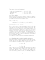
2
A short introduction to the p2 model
The p2 model is designed for statistical analysis of social networks.
Social networks consist of actors and variables indicating their ties.
Often ties simply are recorded by asking actors with whom they have
ties. However, there are many possible measures for ties and actors
do not necessarily have to be persons, but could also be firms, countries, etc. The p2 model analyzes complete networks. This means
that within the networks everyone can possibly be tied to everyone
else, although information on the presence of some ties are allowed
to be missing. In practice, this is the case in closed settings, e.g.
villages, organizations or school classes. The p2 model allows for
some observations from these complete networks to be missing.
2.1
Network data
The p2 model analyzes dichotomous network data, representing ties
that are either present (1) or absent (0). The data are collected in
a square adjacency matrix Y with elements yij indicating a relation
from actor i directed towards actor j (i indicates rows and j columns
in Y ). Below, an example of an adjacency matrix (Y ) indicating the
relations between actors a, b, c, and d is shown:
a
b
c
d





a
0
1
1
0
b
1
0
0
1
c
0
1
0
0
d
0
0
1
0





From such an adjacency matrix, dyads can be derived (Wasserman
& Faust, 1994). A dyad consists of two tie indicator variables Y for
two directed ties between two actors, usually denoted by Dij = (yij ,
yji )= (y1 , y2 ).
3
Three types of dyads are distinguished:
reciprocated (or mutual) dyad → (ya,b , yb,a )= (1, 1)
asymmetric dyad
→ (ya,c , yc,a )= (0, 1)
null dyad
→ (ya,d , yd,a )= (0, 0)
2.2
The p1 model
The p2 model can be seen as an extension of the p1 model introduced by Holland and Leinhardt (1981). The p1 model specifies the
probability for dyads in a network with n actors:
P (Yij = y1 , Yji = y2 )
= exp{y1 (µ + αi + βj ) + y2 (µ + αj + βi ) + y1 y2 ρ}/kij ,
for y1 , y2 = 0, 1; i, j = 1, . . . , n; i 6= j.
Here, ρ can be seen as a reciprocity parameter, since it is the only
term that is involved when ties in both directions are present. The
parameter µ can be recognized as an overall density parameter. For
sender i in the tie indicator variable yij , αi can be seen to be a sender
parameter. For sender j in the opposed tie indicator variable yji , αj
can again be seen as a sender parameter. In a similar manner, the
parameters βj and βi can be recognized as a receiver parameter for
the tie indicator variables yij and yji , respectively. The parameter
kij is a normalizing constant.
Note that in the p1 model the dyads are mutually independent.
2.3
Extending the p1 model to include covariates: p2
The p2 model allows covariates as predictors for the sender, receiver,
density, and reciprocity effects. Within the p2 model the sender and
receiver effects are reformulated, using a regression model, as:
α = X1 γ1 + A,
and
β = X2 γ2 + B,
where α and β are vectors containing the sender and receiver effects
and X1 , X2 are matrices with covariates for the sender and receiver
effects with coefficients γ1 and γ2 , respectively. A and B are random effects with (co)variances σA2 , σB2 , σAB and E(A)= E(B)= 0.
4
Between actors the random effects are assumed independent.
These substitutions can be regarded as a bivariate regression model
for the pairs (αi , βi ).
Replacing the sender and receiver effects by a function of covariates
and random effects, reduces the number of parameters to be estimated. This allows the density and reciprocity parameters to vary
over the dyads. In the p1 model this was not allowed. The density
and reciprocity parameters are reformulated as:
µij = µ + Z1ij δ1 ,
and
ρij = ρ + Z2ij δ2 ,
where Z1ij , Z2ij are matrices containing dyadic attributes for the
density and the reciprocity effects with δ1 and δ2 vectors containing coefficients for the density and reciprocity effect, respectively.
(Dyadic attributes have values for each pair of actors, i, j = 1, . . . , n,
i 6= j.) µ And ρ are the constant parts of µij and ρij . Because ρij
represents reciprocity, ρij = ρji is assumed and therefore the dyadic
attributes that are used as covariates for the reciprocity parameter
are supposed to be equal as well (Z2ij = Z2ji ).
2.4
Dyadic attributes (Zij )
Covariates for the density and reciprocity parameters can vary over
dyads. Hence, they are called dyadic attributes. They can be represented by a matrix. For attributes that are covariates for the
reciprocity parameter, the matrix must be symmetrical.
Dyadic attributes can be collected for each combination of actors
(each dyad), like network data are collected. Dyadic attributes can
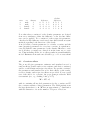
be derived from actor attributes as well. We often use differences
and absolute differences of actor attributes in dyads. Below, there
is an example with two male (coded ’1’) and two female (coded ’0’)
actors. Both the difference between the actors and the absolute difference derived from this dummy variable are illustrated. (Of course,
there are more possibilities for deriving dyadic attributes from actor
attributes.)
5
actor
sex dummy
a
male
1
b
male
1
c
female
0
d
female
0
difference
0 0 1 1
0 0 1 1
-1 -1 0 0
-1 -1 0 0
absolute
difference
0 0 1 1
0 0 1 1
1 1 0 0
1 1 0 0
Note that when covariates for the density parameter are derived
from actor attributes, either the difference or the absolute difference can be applied. For covariates for the reciprocity parameter,
only the absolute difference can be used, since this derivation is symmetrical regarding both directions of the dyads.
A model with a certain parameter for a sender covariate and the
same (negative) parameter for a receiver covariate, is equivalent to
a model with the same parameter for the density difference covariate if all these covariates are derived from the same actor covariate. Thus including all the above effects results in an unidentifiable
model. Estimates from such a model will be poor. Do not use them!
2.5
Covariate effects
The p2 model gives parameter estimates and standard errors for
random effects (sender and receiver variance and their covariance)
and for overall density and reciprocity effects. For specific covariates,
the parameters and standard errors for their effects on the sender,
receiver, density, and reciprocity effects are provided. For an overall
test of the effect of a covariate, the p2 program provides the Wald
test statistic (see, e.g., Serfling, 1980, p. 157):
W = θ̂0 V̂−1 θ̂,
with θ containing all involved parameters for the covariate and V̂
the covariance matrix of these parameters. The Wald statistic tests
the hypothesis that θ = 0. W has an approximate χ2 distribution
with the dimension of θ as the number of degrees of freedom.
6
3
Getting started
To run the p2 program within StOCNET, specific actions are required. These are in short:
1.
2.
3.
4.
5.
6.
7.
Select network data
If necessary, recode network data to be dichotomous (0/1)
Select p2 model and files required for analysis
Specify the model
If necessary, use the advanced model specification
Run p2
View results
In the next sections we will treat an example. The example will be
discussed in a text box, like this one.
We will treat an example of an analysis using p2 on network data
concerning ties between American lawyers. This is a subsection of
the data treated in Lazega and Van Duijn (1997).
Ties represent lawyers seeking advice among 35 partners of a law
firm in two offices. Lawyers indicated to whom they go for advice.
Actor attributes are ’seniority rank number’ (starting with ’1’ for
the highest rank and ending with ’35’ for the lowest rank) and
’office’, the office in which the lawyers work (coded by ’0’ and ’1’)
as covariates.
We also use a dyadic attribute ’cowork’ for which the lawyers were
asked with whom they have worked together.
7
4
Input data
The p2 model is a model for the analysis of binary network data.
This means that the dependent variable in the analysis needs to be a
binary coded network. This network data is expected to be a square
matrix with elements (i,j) representing a tie indicator variable for a
tie from actor ’i’ towards actor ’j’ (i indicates rows and j columns).
A tie has to be represented by ”1”, the absence of a tie by ”0”.
Elements on the diagonal of the network data representing ties from
actors towards themselves are not considered by the p2 model, but
are advised to be set to ”0” for clarity.
If you do not have a binary coded network file, the network data can
easily be transformed to the required binary format within StOCNET. For this option, see the StOCNET manual, Boer et al. (2002).
Covariates can either be actor attributes or dyadic attributes. Note
that networks can be dyadic attributes as well. Separate files are
expected for actor attributes and networks. Dyadic attributes derived from actor attributes (e.g. difference and absolute difference,
see section 2.4) are generated by the p2 program and do not need
to be in a separate file. Covariates are not restricted to particular
values. Thus when network files are used as dyadic attribute, they
are not restricted to binary values.
Note that the actor attributes and the dyadic attributes are supposed to cover the same actors as the dependent network. Thus the
ordering of actors in all these files should be identical.
All data files should only contain data and all values have to be
separated by tabs or spaces. If there is additional information in
the files (e.g. variable names in the first line), the program will not
work. Files are expected to be in ascii format with actors on subsequent lines and different values on a single line.
For each session, StOCNET asks the user to select files containing
network data and files containing actor attributes. Here, select all
the files that you want to use in different analyses. For specific analyses, StOCNET will ask the user which network is the dependent
variable and which files containing actor attributes have to be used.
8
5
Model selection
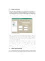
Under the button ’StOCNET model’ (step four in StOCNET), select the p2 model in the pull-down menu in the box ’model choice’.
After the p2 model has been selected, the available network files and
actor attribute files are displayed. From these files, select those that
contain information that you want to use in the analysis. This will
enable specification of covariates later on in the analysis.
model selection window
Select one of the available network files under ’Digraph’. This network will then be the dependent variable in the analysis. If present,
remaining networks can be selected as dyadic covariates. Further,
select the attribute files that contain the actor attributes to be used
as covariates in the analysis.
Pressing ’Model specification’ will allow you to specify your model.
Pressing ’Run!’ starts the p2 estimation process. If you have not
specified a model, the empty model will be estimated on the network that is the dependent variable. We advice to estimate the
empty model first in each new session. This provides a baseline
model for models with covariate effects.
6
Model specifications
In ’model specifications’, specify which covariates to include in the
model. Covariates for the density, reciprocity, sender, and receiver
9
effects can be specified. As mentioned before, covariates for the
density and reciprocity effects are called dyadic attributes. In the
upper half of the ’model specifications’ screen the dyadic attributes
are displayed. These are dyadic attributes derived from actor attributes (differences and absolute differences over dyads) as well as
selected network files. In the lower half of the ’model specifications’
screen actor attributes are displayed. These are the possible covariates for the sender and receiver effects. Marking the checkboxes in
front of any of the covariates will include them in the model.
Note that including a sender and receiver effect for a covariate corresponds to including a density difference effect for this covariate.
Including all the above effects results in an unidentifiable model.
Estimates from such a model will be poor. Do not use them!
model specifications window
Pressing the button ’advanced’ will open the screen with ’advanced
P2 options’. Here, all selected covariates are displayed. Marking the
checkbox in front of these will fix the parameter of the covariate to
a certain value. The value to which the parameter is fixed can be
entered on the right of the covariate name. Novice users are advised
not to use this option.
10
Below these options, a choice for the convergence criterion can be
entered. Either the number of iterations or a measure for convergence can be entered. The measure for convergence is the maximum
difference of all parameter estimates with the estimates from the previous iteration cycle.
advanced model specifications window
11
7
Output
The output of the p2 program is displayed automatically in StOCNET after the iteration process has finished. For a new session, the
output will be visible immediately. For an analysis in an existing
session, the output will be appended to the previous output from
this session. Then, in the output screen of StOCNET, scroll down
to find the output of the last analysis.
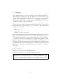
The p2 output is organized in several parts. First there is some basic
information; the version number of p2 , the name of the output file,
and the date and time:
P2 Version 2.0.0.6
example.out
December 17, 2002, 3:26:52 PM
General information on the specific analysis is provided afterwards.
First, the digraph (the network that is the dependent variable in
the analysis) is indicated. Second, the number of valid tie indicator variable observations is printed. Note that this depends on the
number of actors in the network and the number of missing values in
the data. Third, the iteration process is summarized. Other possible messages state the assigned number of iterations and the largest
difference of parameter estimates between the last two performed
iterations.
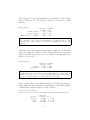
General Information:
Digraph: C:\program files\stocnet\ADVICE35.DAT
Number of valid tie indicator observations: 1190
Convergence criterion: 0.0001 reached after 8 iterations.
In this example the dependent network is advice.dat. From the number of valid tie
indicator observations it is clear that there are no missing values in this dataset. Since
the number of actors is 35, the total number of (directed) tie indicator observations
is 35 × 34 = 1190. Thus, all possible tie indicator observations are valid.
12
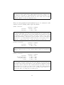
The next part of the output displays the variances of the random
effects. These are σA2 , σB2 , and σAB , referred to in section 2 of this
manual:
Random effects:
parameter
estimate
sender variance:
0.7332
receiver variance:
0.6920
sender receiver covariance: -0.3543
standard
error
0.1633
0.1561
0.1227
Here the amount of variation in sender and receiver activity is presented. That is,
after controlling for the covariates in this analysis. Note that these effects covary
negatively; the more lawyers tend to seek advice, the less likely it is advice is sought
from them.
Following, the output displays fixed effects. First the overall fixed
effects are displayed. These are the overall density and reciprocity
effects as mentioned in section 2. For details on interpreting these
effects, see section 8.
Overall effects:
parameter
estimate
Density: -1.3079
Reciprocity:
1.2648
standard
error
0.3884
0.2994
The negative value of the density parameter indicates that the probability of a relation
is smaller than 0.5 (see section 8) for covariate values equal to zero. The reciprocity
parameter is positive, but not very large, indicating that advice relations have a
tendency to be symmetrical, but not an extremely strong tendency.
Below are the values of the Wald statistic (see section 2) and the pvalues under the approximating χ2 distribution. The Wald statistic
combines the separate t-tests for each covariate.
Overall covariate effects:
Overall effects of covariates including diff and absdiff manipulations.
Covariate
seniority
office
cowork
Wald test
statistic
25.2689
25.3851
133.8964
13
df
3
2
1
P
0.0000
0.0000
0.0000
The covariate seniority is used four times as covariate (sender, receiver, and density
effects). Above is the combined effect of all the instances it was used. Office was used
twice and and cowork just once. The interpretation of these effects should be based
on the specific covariate effects that are shown below. All covariate effects are highly
significant. (This is, of course, not always the case.)
Below are the parameters and standard errors of covariates for the
sender, receiver, density, and reciprocity effects.
Sender covariates:
Covariate
seniority
parameter
estimate
0.0528
standard
error
0.0162
The seniority rank number is positively related to seeking advice. Thus, the higher
the seniority rank number (i.e. the lower the seniority!), the more lawyers tend to
seek advice. More senior lawyers seek less advice than less senior lawyers. Note that
the magnitude of the parameters is related to the range of values of the covariate,
just like unstandardized coefficients in regression analysis. Here the rank numbers
range from 1 to 35. At first sight the parameter may not seem very large. However,
taking into account the range of the covariate, the parameter is rather large.
Receiver covariates:
Covariate
seniority
parameter
estimate
-0.0497
standard
error
0.0160
The seniority rank number is negatively related to advice being sought. Thus, more
advice is sought from the more senior lawyers (lawyers with a low seniority rank
number).
Density covariates:
Covariate
abs_diff_seniority
abs_diff_office
cowork
parameter
estimate
-0.0368
-0.9102
2.0056
standard
error
0.0096
0.2240
0.1733
The negative effect of the absolute difference in seniority rank number indicates that
the probability of an advice relation decreases as the difference in seniority increases.
The negative effect of the absolute difference of the office indicates that the probability
of an advice relation outside the office is smaller than the probability of an advice
relation within one’s own office. Cowork is a dyadic covariate where lawyers indicated
whether they work together with someone else. Working together with someone
increases the chance of seeking advice from that person.
14
Notice that less senior lawyers tend to seek advice more and that advice is sought more
from more senior lawyers. Thus advice appears to ’flow’ from more senior lawyers to
less senior lawyers. Considering this, a positive effect for the difference of seniority
rank would be expected (lawyers with a large rank number seek more advice from
lawyers with a low rank number). Leaving out seniority rank as sender and receiver
covariate will indeed display this effect. Recall from section 2 that for the same
covariate including a sender and receiver effect is equivalent to including a density
difference effect.This problem of unidentifiability is comparable to the collinearity
problem in regression analysis. You are kindly invited to try including covariates
for the different effects to gain more insight in this phenomenon). Section 9 of this
manual deals with this problem as well.
Reciprocity covariates:
Covariate
abs_diff_office
parameter
estimate
0.3365
standard
error
0.4763
Here, there is no increased probability for reciprocal relations as an effect of the
absolute difference of office. Thus here the degree to which advice is a symmetric
relation is not dependent on working in the same office.
15
8
Formulas for effects
In the output of the p2 program parameter estimates are given with
their standard errors. Dividing the former by the latter gives the
t-test statistic. This is the test statistic for the null hypothesis that
the parameter is zero. A commonly used rule of thumb is to accept that the parameter deviates from zero if the absolute value
of the parameter estimate divided by the standard error is two or
larger. More informative are the magnitude and sign of parameters.
Note that the magnitude of parameters for covariates depends on
the range of values of the covariates.
The density and reciprocity parameters have special formulas for
their effects. The density parameter µ can be seen as a log-odds.
The reciprocity parameter ρ can be viewed as the log of an oddsratio.
The definition of µij is the log of the odds:
P (Yij = 1|Yji = 0)/P (Yij = 0|Yji = 0)
i, j = 1, . . . , n; i 6= j .
The definition of ρij is the log of the ratio:
P (Yij = 1|Yji = 1)/P (Yij = 0|Yji = 1)
P (Yij = 1|Yji = 0)/P (Yij = 0|Yji = 0)
=
P (Yij = 1, Yji = 1)P (Yij = 0, Yji = 0)
P (Yij = 1, Yji = 0)P (Yij = 0, Yji = 1)
i, j = 1, . . . , n; i ≤ j.
i, j = 1, . . . , n; i ≤ j.
It represents the log of the increase in the odds that Yij = 1 given
that Yji = 1. The second expression for ρij shows that a higher
value of ρ not only indicates an increased probability of a mutual
tie (1,1), but also indicates an increased probability of a null dyad
(0,0). Thus ρ is a parameter for both symmetric types of dyads (null
and mutual).
As you can see, the density and reciprocity effects are intertwined.
Note that the above interpretations are valid when no covariates are
included in the model. When covariates are added to the model the
same interpretations hold, but only for actors with the same values
on the covariates.
16
9
Limitations
The p2 model has practical limitations for applying it and some more
fundamental limitations concerning the estimation procedure.
A practical limitation may occur when two or more parameters ”estimate” the same information. This will result in unidentifiable estimates, possibly causing overflow (implausibly large estimates). The
same kind of problem is encountered with collinearity in regression
analysis.
Selecting parameters for the sender effect, receiver effect, and density difference effect for the same covariate will result in this problem. In this case it is commonly observed that the convergence
criterion gets stuck at a certain value.
The same problem may arise when a covariate carries very little information. This may be the case when most actors have the same
value. Then again information that a covariate does not contain
may intended to be estimated from the covariate.
Another practical limitation is the maximum number of actors in
the network. Up to version 2.0.0.4 the maximum number of actors
is 90. Note, however, that the number of observations of the tie
indicator variables grows almost quadratically with the number of
actors. So does the computing time. Therefore, when using large
networks, expect long computing times.
For version 2.0.0.5 and higher we estimate the maximum number
of actors to be 180. For 150 actors we know for sure that the program runs satisfactorily. However, expect long computing times for
large networks. In the future we hope to optimize the computing
procedure further and consequently shorten computing time.
A more fundamental problem lies in the estimation procedure applied by the p2 program. The p2 model is a generalized linear mixed
model (thus applying a non-linear link function). The p2 program
uses an IGLS estimation procedure that applies a first order Taylor
approximation of the non-linear link function (see Van Duijn, 1995,
for a similar approach, see e.g. Goldstein, 1991). Such a procedure
has been shown to sometimes underestimate variances in non-linear
mixed models (Rodriguez and Goldman, 1995). In the near future
we hope to offer alternative estimation procedures for the p2 model.
17
Part II
Working with the p2 executable
10
p2 files
The p2 program creates several files. All these files will carry the
session name with different extensions.
Actors are assigned numbers according to their order in the network
file. This ordering should correspond to the ordering of actors in the
files containing actor attributes and dyadic attributes. Information
from all the above files is combined in one single data file. This
file has the extension ’.dat’. Which files contain the required data
(dependent network, covariates, and covariate networks) along with
additional information is stored in the input file. This file has the
extension ’.in’. The model specification is stored in the (model-)
design file. This file has the extension ’.des’.
10.1
the data file
Within the p2 program the data file is created automatically. In
the data file each dyad is represented on two lines; one line for each
directed tie indicator variable in a dyad.
In the data file, each entry on a line carries specific information.
Entries need to be separated by spaces. In the first two entries in
the data file the numbers (according to their order) of the actors
are displayed. Each dyad is represented in two lines. The first line
refers to the ’first’ tie indicator variable, (Yij ), indicating a tie from
the actor on the first entry towards the actor on the second entry. The second line refers to the ’second’, reversed tie indicator
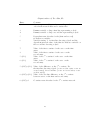
variable, (Yji ). Below there is an overview of the contents of the
data file (with actor covariates c = 1, . . . , C and network covariates
d = 1, . . . , D).
18
Organization of the data file
Entry
1, 2
Contents
Actors, represented by numbers according to their
order in the network files and covariate files
3
4
Dummy variable coding a first line representing a dyad
Dummy variable coding a second line representing a dyad
5
Dependent network value for the (first and second)
tie indicator variables
Variable stating ’1’ for first line denoting a dyad and the
dependent network value of the first tie indicator variable on
the second line denoting a dyad
6
7
8
5+(2*c)
6+(2*c)
Value of the first covariate for the actor on the first
entry
Value of the first covariate for the actor on the
second entry
Value of the cth covariate for the actor on the first
entry
Value of the cth covariate for the actor on the
second entry
Value of the difference on the cth covariate. For
the first line denoting a dyad: (actor on first entry- actor on
second entry), for second line: (actor on second entry- actor
on first entry).
6+(2*C)+(2*c) Value of the absolute difference on the cth covariate
between actors on the first and second entry.
5+(2*C)+(2*c)
6+(2*C)+d
Covariate network value for the dth covariate network.
19
1
1
3
3
2
2
2
1
1
3
1
0
1
0
1
0
1
0
1
0
1
1
0
0
0
1
1
1
0
1
1
1
3
3
2
2
2
1
1
3
0
0
1
1
0
0
0
0
0
1
-1
1
2
-2
-1
1
1
2
2
1
0
0
1
-1
-1
0
0
1
1
1
0
0
0
0
0
Part of the data file for the example presented in the previous sections. There are two actor covariates: ’seniority rank number’ (note
that actors are ordered according to this covariate), and ’office’.
There is one network covariate: ’cowork’.
Each time you run the p2 program, this data file will be produced.
Whenever the same dependent network file and covariate files (actor and dyadic attribute) are selected, the data file will be identical.
Perhaps this seem somewhat wasteful, but this operation takes just
a minimal amount of time. For every differently specified analysis
(with effects for different covariates), different parts of the data file
will be used.
10.2
the input file
For creating the data file, the p2 program needs to know in which files
to find the dependent network, the covariates, and the networks that
are covariates. For creating the output file, the p2 program needs
to know the names of the dependent network and all the covariates.
This information is stored in the input file. For an example, see
Appendix A.
Within StOCNET, the input file is created automatically from the
information entered through the StOCNET interface. The input file
consists of lines that are reserved for specific information.
20
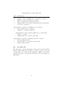
Organization of the input file
Line
1
1
1
2
3
Information
number of actors (+ space)
number of files containing actor covariates (+ space)
number of networks that are covariates
File containing the dependent network
Missing value codes for the dependent network (separated
by spaces) (optional)
subsequently, for all files containing actor covariates:
∗
file containing actor covariates
∗
Number of covariates in the file
subsequently, for all covariates within actor covariate files:
∗ Name of covariate
∗ Missing value for covariate (optional)
subsequently, for all files containing network covariates:
∗
file containing network
∗
missing values for the network (optional)
∗
name for the network
10.3
the design file
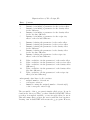
The design file contains information on how the model is specified.
That is, which effects are specified for which covariates. For each
covariate there is one line in the design file. Entries on the lines,
separated by spaces, carry specific information. For an example, see
appendix B.
21
Organization of the design file
Entry
1
2
3
4
5
6
7
8
9
10
11
12
13
14
15
Contents
Dummy for including a parameter
Dummy for including a parameter
Dummy for including a parameter
for the difference
Dummy for including a parameter
for the absolute difference
Dummy for including a parameter
effect for the absolute difference
Dummy for fixing the parameter
Dummy for fixing the parameter
Dummy for fixing the parameter
for the difference
Dummy for fixing the parameter
for the absolute difference
Dummy for fixing the parameter
effect for the absolute difference
for the sender effect
for the receiver effect
for the density effect
for the density effect
for the reciprocity
for the sender effect
for the receiver effect
for the density effect
for the density effect
for the reciprocity
Value on which to fix the parameter
Value on which to fix the parameter
Value on which to fix the parameter
(difference)
Value on which to fix the parameter
(absolute difference)
Value on which to fix the parameter
effect (absolute difference)
for the sender effect
for the receiver effect
for the density effect
for the density effect
for the reciprocity
subsequently, after lines for all covariates:
∗
assigned number of iterations
∗
convergence criterion
∗
dummy for using the assigned number of iterations(1)
or the convergence criterion (0)
The executable of the p2 program is simply called p2.exe. It can be
found in the directory where you have installed StOCNET. Whenever there is an update available, you are strongly advised to use it.
This will ensure that you have the version with the best bug fixes.
Pressing ’run’ in StOCNET will execute the p2 program. However,
22
if you have specified the input file and the design file correctly, the
p2 executable will work outside StOCNET as well.
If the p2 program is used within StOCNET, references to files containing networks and covariates will be altered. The original filenames will preceded by a tilde (˜) . This is because StOCNET has
the option for selecting specific actors (step 3; Selection). Therefore, StOCNET produces a new file with the name of the old file,
preceded by a tilde. In StOCNET, it is this file that is referred to.
11
Creating dyadic covariates for specific values
of actor attributes
Sometimes the standard options of the p2 program will not be satisfactory. Suppose you find a negative effect for the absolute difference of sex on the density (of relations). Roughly, this means
that relations are less likely between actors of a different sex and
consequently more likely when actors share the same sex. Now, you
may wonder whether relationships between boys are equally more
likely as relationships between girls. The common analysis with p2
will not provide an answer to that question. What would provide
an answer to that question is a network covariate coding whether
dyads concern both boys or both girls (instead of just coding the
same sex). This is what we mean by creating dyadic covariates for
specific values of actor attributes. Note that this can be done for
the density effect and for the reciprocity effect.
With some extra effort, the p2 program can be used to create dyadic
covariates indicating equality for specific values of actor covariates.
To do this the input file and the design file need to be altered. These
altered files can be used by the p2 executable (outside StOCNET!)
to create network files containing such dyadic covariates. Of course
there are many other possibilities to produce a dyadic covariate indicating equality for a specific value of a covariate. How a dyadic
covariate was produced, makes no difference to the p2 program.
11.1
adjusting the input file
The first thing to do when you want to create a new network file
for a specific value of an actor attribute is entering a ’1’ on the first
empty line of the input file (that is, after the last non-empty line).
This is a dummy indicating you want to create this file.
23
On the next line you enter the name of the variable you want to
compute the new network file from.
On the next line enter the value for which you want to create the file.
For this specific value the new network file will contain a ’1’ only
if both actors have this specific value. Otherwise, the new network
file will contain a ’0’.
On the last line, enter the name of the new file. This should be a
full name, including an extension (assuming that is what you want).
After taking the previous actions, the original input file should on
the bottom part have something like the following added:
1
office
1
boston.net
After running the analysis, you will have a new network file (here:
boston.net). If you do not want to create the new network file again,
skip the above lines and add the network file to the other files in
your analysis. This can either be done in StOCNET (see StOCNET
manual or section 4 of this manual) or in the input file (see section
10.2).
11.2
adjusting the design file
The p2 program immediately recognizes the new network file as a
covariate. Thus you have to add a line with 15 entries (see section
10.2) on the bottom of the design part of the design file. If you want
to estimate parameters for the newly created dyadic covariate, enter
a ’1’ on the third entry for density and on fifth entry for reciprocity.
All other entries have to be ’0’ unless you want to fix the parameter
to a certain value (see section 10.3).
11.3
running p2
When creating a new network file for a specific value of an actor
attribute, the p2 program cannot be run from within StOCNET.
The easiest way to do this is by creating a shortcut to ’p2.exe’. In
the properties of the shortcut, there are some changes needed. After
the path, enter a space and the title of your session. This should
look like:
"C:\Program Files\p2\p2.exe" example
24
The shortcut should start in the directory where the input file and
design file are stored. If this is not the case, this should also be
changed in the properties of your shortcut.
If ’p2.exe’, the input file, and the design file are stored in the same
directory, entering:
p2 example
and hitting enter in your (Windows) Dos-emulator will work as well.
25
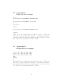
12
Appendix A:
Input file for example
35 1 1
C:\Program files\StOCNET\~ADVICE35.DAT
C:\Program files\StOCNET\~covp2.dat
2
seniority
office
C:\Program files\StOCNET\~COWORK35.DAT
cowork
Input file for the example first presented in section 3. There are
two actor covariates (from the same file): ’seniority rank number’
(note that actors are ordered according to this covariate), and ’office’. There is one network covariate: ’cowork’.
13
Appendix B:
Design file for example
1 1 0 1 0 0 0 0 0 0 0 0 0 0 0
0 0 0 1 1 0 0 0 0 0 0 0 0 0 0
0 0 1 0 0 0 0 0 0 0 0 0 0 0 0
200
0.0001
0
Design file for the example first presented in section 3. There are
two actor covariates (from the same file): ’seniority rank number’
(note that actors are ordered according to this covariate), and ’office’. There is one network covariate: ’cowork’.
26
14
References
Boer, P., Huisman, M., Snijders, T.A.B., & Zeggelink, E.P.H.
(2001). StOCNET: an open software system for the advanced statistical analysis of social networks. Groningen: ProGAMMA / ICS.
Website: http://stat.gamma.rug.nl/stocnet.
Boer, P., Huisman, M., Snijders, T.A.B., & Zeggelink, E.P.H.
(2002). StOCNET user’s manual Version 1.3. Available from website: http://stat.gamma.rug.nl/stocnet.
Goldstein, H. (1991). Nonlinear multilevel models, with an application to discrete response data. Biometrika, 78, 45–51.
Serfling, R.J. (1980). Approximation Theorems of Mathematical
Statistics. New York: John Wiley & Sons.
Lazega, E. & Van Duijn, M. (1997). Position in formal structure,
personal characteristics and choices of advisers in a law firm: a logistic regression model for dyadic network data. Social Networks,
19, p. 375- 397.
Rodriguez, G. & Goldman, N (1995). An assessment of estimation procedures for multilevel models with binary responses. Journal
of the Royal Statistical Society, A, 158, 73-89.
Van Duijn, M.A.J., 1995. Estimation of a random effects model
for directed graphs. In: Snijders, T.A.B. et al. (Ed.) SSS ’95.
Symposium Statistische Software, nr. 7. Toeval zit overal: programmatuur voor random-coffcint modellen, p. 113–131. Groningen, iec
ProGAMMA.
Wasserman, S. & Faust, K. (1994). Social Network Analysis:
Methods and Applications. Cambridge: Cambridge University Press.
27