Download ST-Realizer-II user manual (for ST62 & ST7 8-bit MCUs)

®
ST-Realizer II
USER MANUAL
June 1999
Ref: DOC-ST-REALIZER-II
USE IN LIFE SUPPORT DEVICES OR SYSTEMS MUST BE EXPRESSLY AUTHORIZED.
STMicroelectronics PRODUCTS ARE NOT AUTHORIZED FOR USE AS CRITICAL COMPONENTS IN
LIFE SUPPORT DEVICES OR SYSTEMS WITHOUT THE EXPRESS WRITTEN APPROVAL OF
STMicroelectronics. As used herein:
1. Life support devices or systems are those
which (a) are intended for surgical implant into
the body, or (b) support or sustain life, and whose
failure to perform, when properly used in
accordance with instructions for use provided
with the product, can be reasonably expected to
result in significant injury to the user.
1
2. A critical component is any component of a life
support device or system whose failure to
perform can reasonably be expected to cause the
failure of the life support device or system, or to
affect its safety or effectiveness.
TABLE OF CONTENTS
1
INSTALLING ST-REALIZER II . . . . . . . . . . . . . . . . . . . . . . . . . . . . . . . . . . . . . . . . . 1
1.1 What You Need to Install ST-Realizer II . . . . . . . . . . . . . . . . . . . . . . . . . . . . . . 1
1.2 Installation Procedure . . . . . . . . . . . . . . . . . . . . . . . . . . . . . . . . . . . . . . . . . . . . 1
1.3 Folders and Sub-folders . . . . . . . . . . . . . . . . . . . . . . . . . . . . . . . . . . . . . . . . . . 2
2
INTRODUCTION AND CONCEPTS . . . . . . . . . . . . . . . . . . . . . . . . . . . . . . . . . . . . . 3
2.1 ST-Realizer Application Structures . . . . . . . . . . . . . . . . . . . . . . . . . . . . . . . . . . 4
2.2 Programming using Symbols . . . . . . . . . . . . . . . . . . . . . . . . . . . . . . . . . . . . . . . 4
2.3 Inside ST-Realizer Applications . . . . . . . . . . . . . . . . . . . . . . . . . . . . . . . . . . . . . 5
2.4 Symbols . . . . . . . . . . . . . . . . . . . . . . . . . . . . . . . . . . . . . . . . . . . . . . . . . . . . . . . 6
2.4.1
State Machine Symbols . . . . . . . . . . . . . . . . . . . . . . . . . . . . . . . . . . . . 6
2.5 Schemes . . . . . . . . . . . . . . . . . . . . . . . . . . . . . . . . . . . . . . . . . . . . . . . . . . . . . . 7
2.5.2
The Root Scheme . . . . . . . . . . . . . . . . . . . . . . . . . . . . . . . . . . . . . . . . 7
2.5.3
Subschemes . . . . . . . . . . . . . . . . . . . . . . . . . . . . . . . . . . . . . . . . . . . . 7
2.6 Events . . . . . . . . . . . . . . . . . . . . . . . . . . . . . . . . . . . . . . . . . . . . . . . . . . . . . . . . 8
2.6.4
Execution Conditions . . . . . . . . . . . . . . . . . . . . . . . . . . . . . . . . . . . . . . 8
2.6.5
Event Symbols . . . . . . . . . . . . . . . . . . . . . . . . . . . . . . . . . . . . . . . . . . . 9
2.7 How ST-Realizer Keeps Track of Time . . . . . . . . . . . . . . . . . . . . . . . . . . . . . . 10
2.8 Connecting your Application to the Target Device . . . . . . . . . . . . . . . . . . . . . 11
2.9 Application Development Steps . . . . . . . . . . . . . . . . . . . . . . . . . . . . . . . . . . . . 11
3
TUTORIAL . . . . . . . . . . . . . . . . . . . . . . . . . . . . . . . . . . . . . . . . . . . . . . . . . . . . . . . 13
3.1 Setting Up Your Project . . . . . . . . . . . . . . . . . . . . . . . . . . . . . . . . . . . . . . . . . . 13
3.1.1
Creating the Project File . . . . . . . . . . . . . . . . . . . . . . . . . . . . . . . . . . 13
3.1.2
Choosing a Target Microcontroller . . . . . . . . . . . . . . . . . . . . . . . . . . . 14
3.1.3
Opening the Main Scheme . . . . . . . . . . . . . . . . . . . . . . . . . . . . . . . . 16
3.1.4
The Worksheet Toolbar . . . . . . . . . . . . . . . . . . . . . . . . . . . . . . . . . . . 16
3.2 Designing and Drawing Schemes . . . . . . . . . . . . . . . . . . . . . . . . . . . . . . . . . . 17
3.2.5
The State Machine Diagram . . . . . . . . . . . . . . . . . . . . . . . . . . . . . . . 18
3.3 Completing the Heating Control Application . . . . . . . . . . . . . . . . . . . . . . . . . . 26
3.3.6
What differentiates a main scheme from a subscheme? . . . . . . . . . . 27
3.3.7
External Input Conditions . . . . . . . . . . . . . . . . . . . . . . . . . . . . . . . . . . 28
3.3.8
Internal Input Conditions . . . . . . . . . . . . . . . . . . . . . . . . . . . . . . . . . . 32
3.3.9
External Actions . . . . . . . . . . . . . . . . . . . . . . . . . . . . . . . . . . . . . . . . . 33
iii
1
Table of Contents
3.3.10
3.3.11
3.3.12
3.3.13
The Creation of a Subscheme for an Internal Event-Driven Action . . 35
Connecting Hardware Ports and Peripherals . . . . . . . . . . . . . . . . . . . 38
Event Control . . . . . . . . . . . . . . . . . . . . . . . . . . . . . . . . . . . . . . . . . . . 41
Summary . . . . . . . . . . . . . . . . . . . . . . . . . . . . . . . . . . . . . . . . . . . . . . 43
3.4 Analysing and Generating Program Code . . . . . . . . . . . . . . . . . . . . . . . . . . . . 44
3.4.14 Setting the Compile Options . . . . . . . . . . . . . . . . . . . . . . . . . . . . . . . 44
3.4.15 Executing the Analysis and Compile . . . . . . . . . . . . . . . . . . . . . . . . . 45
3.4.16 Viewing the Analyse and Compile Report . . . . . . . . . . . . . . . . . . . . . 46
3.5 Simulating and Fine-Tuning Your Application . . . . . . . . . . . . . . . . . . . . . . . . . 47
3.5.17 Creating the Simulation Environment File (.sef) . . . . . . . . . . . . . . . . 47
3.5.18 Connecting Probes and Adjusters . . . . . . . . . . . . . . . . . . . . . . . . . . . 48
3.5.19 Running the Simulator . . . . . . . . . . . . . . . . . . . . . . . . . . . . . . . . . . . . 53
3.6 Now it’s Up to You! . . . . . . . . . . . . . . . . . . . . . . . . . . . . . . . . . . . . . . . . . . . . . 53
4
CREATING, OPENING AND SAVING PROJECTS . . . . . . . . . . . . . . . . . . . . . . . . 55
4.1 Project Files . . . . . . . . . . . . . . . . . . . . . . . . . . . . . . . . . . . . . . . . . . . . . . . . . . . 55
4.2 Creating a New Project . . . . . . . . . . . . . . . . . . . . . . . . . . . . . . . . . . . . . . . . . . 55
4.3 Opening an Existing Project . . . . . . . . . . . . . . . . . . . . . . . . . . . . . . . . . . . . . . 56
4.4 Opening Earlier Realizer Version Projects . . . . . . . . . . . . . . . . . . . . . . . . . . . 56
4.5 Closing a Project . . . . . . . . . . . . . . . . . . . . . . . . . . . . . . . . . . . . . . . . . . . . . . . 57
4.6 Saving Projects . . . . . . . . . . . . . . . . . . . . . . . . . . . . . . . . . . . . . . . . . . . . . . . . 57
5
SPECIFYING THE TARGET HARDWARE DEVICE . . . . . . . . . . . . . . . . . . . . . . . 59
5.1 ST6 or ST7 Devices . . . . . . . . . . . . . . . . . . . . . . . . . . . . . . . . . . . . . . . . . . . . 59
5.2 Choosing a Target Microcontroller . . . . . . . . . . . . . . . . . . . . . . . . . . . . . . . . . 60
5.2.1
Selecting the Target Microcontroller for a New Project . . . . . . . . . . . 60
5.2.2
Changing the Target Microcontroller . . . . . . . . . . . . . . . . . . . . . . . . . 61
5.3 Hardware Configuration . . . . . . . . . . . . . . . . . . . . . . . . . . . . . . . . . . . . . . . . . . 62
5.3.3
Accessing Hardware Settings Dialog Boxes . . . . . . . . . . . . . . . . . . . 62
5.3.4
General Hardware Configuration . . . . . . . . . . . . . . . . . . . . . . . . . . . . 63
5.3.5
Memory Configuration . . . . . . . . . . . . . . . . . . . . . . . . . . . . . . . . . . . . 65
5.3.6
Enabling Peripherals . . . . . . . . . . . . . . . . . . . . . . . . . . . . . . . . . . . . . 66
6
CREATING, OPENING, SAVING SCHEMES . . . . . . . . . . . . . . . . . . . . . . . . . . . . . 67
6.1 Schemes . . . . . . . . . . . . . . . . . . . . . . . . . . . . . . . . . . . . . . . . . . . . . . . . . . . . . 67
6.2 Creating a New Scheme . . . . . . . . . . . . . . . . . . . . . . . . . . . . . . . . . . . . . . . . . 67
6.2.1
Opening the Root Scheme . . . . . . . . . . . . . . . . . . . . . . . . . . . . . . . . . 67
6.2.2
Creating Subschemes and other Schemes . . . . . . . . . . . . . . . . . . . . 68
6.3 Opening a Scheme . . . . . . . . . . . . . . . . . . . . . . . . . . . . . . . . . . . . . . . . . . . . . 69
6.4 Saving Schemes . . . . . . . . . . . . . . . . . . . . . . . . . . . . . . . . . . . . . . . . . . . . . . . 69
iv
Table of Contents
7
BUILDING SCHEMES . . . . . . . . . . . . . . . . . . . . . . . . . . . . . . . . . . . . . . . . . . . . . . 71
7.1 Schemes and their Components . . . . . . . . . . . . . . . . . . . . . . . . . . . . . . . . . . . 71
7.2 Symbols . . . . . . . . . . . . . . . . . . . . . . . . . . . . . . . . . . . . . . . . . . . . . . . . . . . . . . 71
7.2.1
Placing and Controlling Symbols . . . . . . . . . . . . . . . . . . . . . . . . . . . . 72
7.2.2
Wiring Symbols Together and Connecting Application Inputs/Outputs 78
7.3 Working in Schemes . . . . . . . . . . . . . . . . . . . . . . . . . . . . . . . . . . . . . . . . . . . . 82
7.4 Subschemes, Execution Conditions and Events . . . . . . . . . . . . . . . . . . . . . . . 85
7.4.3
Description of ST-Realizer Events . . . . . . . . . . . . . . . . . . . . . . . . . . . 85
7.4.4
Execution Conditions . . . . . . . . . . . . . . . . . . . . . . . . . . . . . . . . . . . . . 89
7.4.5
Event Symbols . . . . . . . . . . . . . . . . . . . . . . . . . . . . . . . . . . . . . . . . . . 89
7.4.6
Compatibilities Between Types of Events and Certain Symbols . . . . 91
7.4.7
Subscheme Operations . . . . . . . . . . . . . . . . . . . . . . . . . . . . . . . . . . . 92
7.5 Table Symbols . . . . . . . . . . . . . . . . . . . . . . . . . . . . . . . . . . . . . . . . . . . . . . . . . 99
8
THE MAIN SYMBOL LIBRARY . . . . . . . . . . . . . . . . . . . . . . . . . . . . . . . . . . . . . . 103
8.1 Input and Output Symbols . . . . . . . . . . . . . . . . . . . . . . . . . . . . . . . . . . . . . . . 103
8.2 Sequential Symbols . . . . . . . . . . . . . . . . . . . . . . . . . . . . . . . . . . . . . . . . . . . . 105
8.3 Logic Symbols . . . . . . . . . . . . . . . . . . . . . . . . . . . . . . . . . . . . . . . . . . . . . . . . 107
8.4 Time Related Symbols . . . . . . . . . . . . . . . . . . . . . . . . . . . . . . . . . . . . . . . . . 116
8.5 Mathematical Symbols . . . . . . . . . . . . . . . . . . . . . . . . . . . . . . . . . . . . . . . . . 118
8.6 Counter Symbols . . . . . . . . . . . . . . . . . . . . . . . . . . . . . . . . . . . . . . . . . . . . . . 120
8.7 Conversion Symbols . . . . . . . . . . . . . . . . . . . . . . . . . . . . . . . . . . . . . . . . . . . 121
8.8 Table Symbols . . . . . . . . . . . . . . . . . . . . . . . . . . . . . . . . . . . . . . . . . . . . . . . . 124
8.9 Power Management . . . . . . . . . . . . . . . . . . . . . . . . . . . . . . . . . . . . . . . . . . . 125
8.10 Constant Symbols . . . . . . . . . . . . . . . . . . . . . . . . . . . . . . . . . . . . . . . . . . . . . 126
8.11 State Machine Symbols . . . . . . . . . . . . . . . . . . . . . . . . . . . . . . . . . . . . . . . . . 126
8.12 Hierarchical Sheet Symbols . . . . . . . . . . . . . . . . . . . . . . . . . . . . . . . . . . . . . 128
8.13 Title Symbols . . . . . . . . . . . . . . . . . . . . . . . . . . . . . . . . . . . . . . . . . . . . . . . . . 128
9
ANALYSING AND GENERATING YOUR APPLICATION . . . . . . . . . . . . . . . . . . 129
9.1 Overview . . . . . . . . . . . . . . . . . . . . . . . . . . . . . . . . . . . . . . . . . . . . . . . . . . . . 129
9.2 Changing the Compile Options . . . . . . . . . . . . . . . . . . . . . . . . . . . . . . . . . . . 129
9.3 Executing the Analysis and Compile . . . . . . . . . . . . . . . . . . . . . . . . . . . . . . . 133
9.4 What to Do if there are Errors Found during Analyse . . . . . . . . . . . . . . . . . . 134
9.5 Viewing and Tracing Generated Messages . . . . . . . . . . . . . . . . . . . . . . . . . . 135
9.5.1
Viewing the Analyse and Compile Report . . . . . . . . . . . . . . . . . . . . 135
v
Table of Contents
9.6 Printing Reports . . . . . . . . . . . . . . . . . . . . . . . . . . . . . . . . . . . . . . . . . . . . . . . 138
10 SIMULATING YOUR APPLICATION . . . . . . . . . . . . . . . . . . . . . . . . . . . . . . . . . . 139
10.1 Working with Simulation Environment Files . . . . . . . . . . . . . . . . . . . . . . . . . 139
10.1.1 Creating a New .sef File . . . . . . . . . . . . . . . . . . . . . . . . . . . . . . . . 139
10.1.2 Opening an Existing .sef File . . . . . . . . . . . . . . . . . . . . . . . . . . . . 141
10.1.3 Saving an .SEF File . . . . . . . . . . . . . . . . . . . . . . . . . . . . . . . . . . . . . 142
10.2 Setting, Adjusting and Viewing Input Values . . . . . . . . . . . . . . . . . . . . . . . . . 142
10.2.4 Setting Fixed Input Values . . . . . . . . . . . . . . . . . . . . . . . . . . . . . . . . 143
10.2.5 Setting Variable Input Values . . . . . . . . . . . . . . . . . . . . . . . . . . . . . . 146
10.2.6 Setting Sinusoidal Input Signals . . . . . . . . . . . . . . . . . . . . . . . . . . . 148
10.2.7 Setting Square Wave Input Signals . . . . . . . . . . . . . . . . . . . . . . . . . 150
10.3 Monitoring Signals with Probes . . . . . . . . . . . . . . . . . . . . . . . . . . . . . . . . . . . 151
10.3.8 Viewing Signal Values Numerically . . . . . . . . . . . . . . . . . . . . . . . . . 152
10.3.9 Viewing Signal Values Graphically . . . . . . . . . . . . . . . . . . . . . . . . . 153
10.3.10 Viewing State Machine States . . . . . . . . . . . . . . . . . . . . . . . . . . . . . 156
10.4 Selecting Adjusters and Probes . . . . . . . . . . . . . . . . . . . . . . . . . . . . . . . . . . 157
10.5 Running the Simulator . . . . . . . . . . . . . . . . . . . . . . . . . . . . . . . . . . . . . . . . . . 157
10.5.11 Starting/Stopping the Simulation . . . . . . . . . . . . . . . . . . . . . . . . . . . 158
10.5.12 Setting Run Options . . . . . . . . . . . . . . . . . . . . . . . . . . . . . . . . . . . . . 158
10.6 Recording and Reusing Adjuster and Probe Values . . . . . . . . . . . . . . . . . . . 160
10.6.13 Recording Adjuster and Probe Values . . . . . . . . . . . . . . . . . . . . . . . 161
10.6.14 Reusing Adjuster Values . . . . . . . . . . . . . . . . . . . . . . . . . . . . . . . . . 162
11 CREATING YOUR OWN SYMBOL . . . . . . . . . . . . . . . . . . . . . . . . . . . . . . . . . . . 165
11.1 Overview . . . . . . . . . . . . . . . . . . . . . . . . . . . . . . . . . . . . . . . . . . . . . . . . . . . . 165
11.2 Running the ST Symbol Editor . . . . . . . . . . . . . . . . . . . . . . . . . . . . . . . . . . . 165
11.3 Defining a New Subscheme Symbol . . . . . . . . . . . . . . . . . . . . . . . . . . . . . . . 166
11.3.1 Adding Your New Subscheme Symbol to a Library . . . . . . . . . . . . . 169
11.4 Defining a New User-Defined Symbol . . . . . . . . . . . . . . . . . . . . . . . . . . . . . . 171
11.4.1 Defining the New Symbol . . . . . . . . . . . . . . . . . . . . . . . . . . . . . . . . . 172
11.4.2 Editing the New Symbol . . . . . . . . . . . . . . . . . . . . . . . . . . . . . . . . . . 176
11.4.3 Adding Pins to Your Symbol . . . . . . . . . . . . . . . . . . . . . . . . . . . . . . 181
11.4.4 Assigning Attributes to Your Symbol . . . . . . . . . . . . . . . . . . . . . . . . 182
11.4.5 Modifying Existing Attributes . . . . . . . . . . . . . . . . . . . . . . . . . . . . . . 185
11.4.6 Creating the Macro Header . . . . . . . . . . . . . . . . . . . . . . . . . . . . . . . 187
11.4.7 Creating the New User-Defined Symbol Macro . . . . . . . . . . . . . . . . 187
11.4.8 Writing the Assembly Macro . . . . . . . . . . . . . . . . . . . . . . . . . . . . . . 188
11.4.9 Adding New User-Defined Symbols to a Library . . . . . . . . . . . . . . . 191
vi
Table of Contents
12 CUSTOMIZING ST-REALIZER . . . . . . . . . . . . . . . . . . . . . . . . . . . . . . . . . . . . . . . 193
12.1 Automatically Saving Your Work and Setting Screen Preference. . . . . . . . . 194
12.2 Attribute Display Preferences . . . . . . . . . . . . . . . . . . . . . . . . . . . . . . . . . . . . 195
12.3 Worksheet Layout Preferences . . . . . . . . . . . . . . . . . . . . . . . . . . . . . . . . . . . 196
12.4 Printing Options . . . . . . . . . . . . . . . . . . . . . . . . . . . . . . . . . . . . . . . . . . . . . . . 197
12.5 Symbol Layout Preferences . . . . . . . . . . . . . . . . . . . . . . . . . . . . . . . . . . . . . 198
12.6 Customizing Toolbars . . . . . . . . . . . . . . . . . . . . . . . . . . . . . . . . . . . . . . . . . . 199
12.6.1 Adding and Deleting Toolbar Buttons . . . . . . . . . . . . . . . . . . . . . . . 200
12.6.2 Placing Separators Between Toolbar Buttons . . . . . . . . . . . . . . . . . 200
12.6.3 Changing the Order of Toolbar Buttons . . . . . . . . . . . . . . . . . . . . . . 200
12.6.4 Restoring the Default Toolbar . . . . . . . . . . . . . . . . . . . . . . . . . . . . . 200
12.7 Wire Drawing Options . . . . . . . . . . . . . . . . . . . . . . . . . . . . . . . . . . . . . . . . . . 201
Appendix A:Variables and Attributes . . . . . . . . . . . . . . . . . . . . . . . . . . . . . . . . . . . . 203
A1
Variable Types and Rules . . . . . . . . . . . . . . . . . . . . . . . . . . . . . . . . . . . . . . . 203
A1.1
Type Inheritance . . . . . . . . . . . . . . . . . . . . . . . . . . . . . . . . . . . . . . . . 204
A1.2
Type Overruling . . . . . . . . . . . . . . . . . . . . . . . . . . . . . . . . . . . . . . . . 205
A2
Attribute Types . . . . . . . . . . . . . . . . . . . . . . . . . . . . . . . . . . . . . . . . . . . . . . . . 205
A2.1
Pin Attributes. . . . . . . . . . . . . . . . . . . . . . . . . . . . . . . . . . . . . . . . . . . 206
A2.2
Symbol Attributes . . . . . . . . . . . . . . . . . . . . . . . . . . . . . . . . . . . . . . . 207
Appendix B:Sample Applications . . . . . . . . . . . . . . . . . . . . . . . . . . . . . . . . . . . . . . . 211
B1
Coded
B1.1
B1.2
B1.3
B1.4
B1.5
Lock Application . . . . . . . . . . . . . . . . . . . . . . . . . . . . . . . . . . . . . . . . . 211
Application Overview . . . . . . . . . . . . . . . . . . . . . . . . . . . . . . . . . . . . 211
Functional Description . . . . . . . . . . . . . . . . . . . . . . . . . . . . . . . . . . . 212
Sequencing Control . . . . . . . . . . . . . . . . . . . . . . . . . . . . . . . . . . . . . 212
Secret Code Storage in the EEPROM . . . . . . . . . . . . . . . . . . . . . . . 214
Access Code Entry and Recognition . . . . . . . . . . . . . . . . . . . . . . . . 214
B2
Analog Multiple Key Decoder . . . . . . . . . . . . . . . . . . . . . . . . . . . . . . . . . . . . . 215
B2.1
Application Overview . . . . . . . . . . . . . . . . . . . . . . . . . . . . . . . . . . . . 215
B2.2
The Keyboard . . . . . . . . . . . . . . . . . . . . . . . . . . . . . . . . . . . . . . . . . . 216
B2.3
Software Generation . . . . . . . . . . . . . . . . . . . . . . . . . . . . . . . . . . . . . 217
B2.4
Possible Improvements. . . . . . . . . . . . . . . . . . . . . . . . . . . . . . . . . . . 218
B3
Clock Design . . . . . . . . . . . . . . . . . . . . . . . . . . . . . . . . . . . . . . . . . . . . . . . . . 220
B3.1
Application Overview . . . . . . . . . . . . . . . . . . . . . . . . . . . . . . . . . . . . 220
B3.2
Current Time Counting . . . . . . . . . . . . . . . . . . . . . . . . . . . . . . . . . . . 220
B3.3
Current Time Setup. . . . . . . . . . . . . . . . . . . . . . . . . . . . . . . . . . . . . . 221
B3.4
Alarm Time Setup . . . . . . . . . . . . . . . . . . . . . . . . . . . . . . . . . . . . . . . 221
B3.5
Alarm triggering. . . . . . . . . . . . . . . . . . . . . . . . . . . . . . . . . . . . . . . . . 221
B3.6
Timebase . . . . . . . . . . . . . . . . . . . . . . . . . . . . . . . . . . . . . . . . . . . . . 221
vii
Table of Contents
B3.7
B3.8
B3.9
B4
Current Time Counting . . . . . . . . . . . . . . . . . . . . . . . . . . . . . . . . . . . 222
Current Time Setup. . . . . . . . . . . . . . . . . . . . . . . . . . . . . . . . . . . . . . 223
Alarm Time Setup . . . . . . . . . . . . . . . . . . . . . . . . . . . . . . . . . . . . . . . 224
Fast Counter Application . . . . . . . . . . . . . . . . . . . . . . . . . . . . . . . . . . . . . . . . 225
B4.1
The Application . . . . . . . . . . . . . . . . . . . . . . . . . . . . . . . . . . . . . . . . . 225
B4.2
Fast Counter Report File. . . . . . . . . . . . . . . . . . . . . . . . . . . . . . . . . . 228
B4.3
Generated Code . . . . . . . . . . . . . . . . . . . . . . . . . . . . . . . . . . . . . . . . 230
INDEX . . . . . . . . . . . . . . . . . . . . . . . . . . . . . . . . . . . . . . . . . . . . . . . . . . . . . . . . . . . . . . 237
viii
Chapter 1
1
What You Need to Install ST-Realizer II
INSTALLING ST-REALIZER II
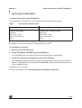
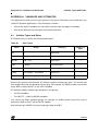
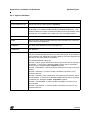
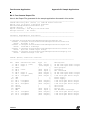
1.1 What You Need to Install ST-Realizer II
You must install ST-Realizer II on a PC that meets the following requirements:
Table 1
PC Hardware Requirements
Minimum requirements
For Optimum Performance
Processor: Intel®80486
Processor: Intel® Pentium-100 MHz
RAM: 8 Mb
RAM: 16 Mb
Disk memory: 14 Mb
Disk memory: 16 Mb
Monitor: Grey scale VGA
Monitor: Super-VGA, 17"
Mouse
Mouse
ST-Realizer II runs under Microsoft® Windows® 95, 98, or NT®.
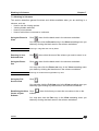
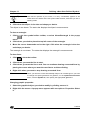
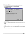
1.2 Installation Procedure
1
Boot your PC under Windows.
2
Put the ST-Realizer CD-ROM in your CD-ROM drive.
The CD-ROM’s autorun function will open the Setup program automatically.
3
Follow the instructions that appear in the pop-up windows.
The Installation program will ask you to specify the folder into which you wish to install STRealizer. The folder you choose will be the root folder. Either accept the default or enter
a new installation folder.
Installation is now complete.
È
È
È
To launch ST-Realizer, click Start Programs ST-Realizer II Realizer.
1/248
Folders and Sub-folders
Chapter 1
1.3 Folders and Sub-folders
The installation process creates the following folders and sub-folders:
<root_folder> which contains the system executable files and DLLs. (The root folder is C:/
Program Files/ST-Realizer/ by default.)
<root_folder>\Examples which contains examples of ST-Realizer projects.
<root_folder>\Help, which contains the help files, a readme file and PDF documents about
ST-Realizer.
<root_folder>\Lib, which contains the main symbol library and a number of other libraries.
<root_folder>\TargetHW, which contains the definition files for the ST6 and ST7
microcontrollers supported by ST-Realizer II.
2/248
Chapter 2
2
INTRODUCTION AND CONCEPTS
The founding idea behind ST-Realizer was to create an accessible and user-friendly software
package, allowing people at various levels of programming expertise to efficiently design
embedded applications for ST6 and ST7 microcontrollers.
ST-Realizer is an application programming package that allows you to create applications
ready to be loaded into ST6 and ST7 microcontrollers without having any knowledge of
assembler code. To do this, you use symbols that represent programming functions to create
flow diagrams that perform your application functions. While the user is assumed to have a
good understanding of the microcontroller for which he or she wishes to create an application,
care has been taken to create a sufficiently broad spectrum of symbols to cover all of your
application design needs. And should you require a symbol not included in ST-Realizer’s main
library, you can design your own using the Symbol Editor function.
All ST-Realizer applications are destined for one of the ST6 or ST7 family of microcontrollers.
The scope of the application is necessarily limited by the resources available on the target
device—the microcontroller for which the application has been designed.
It is therefore imperative that you fully understand the specifications of the target
microcontroller before you begin to design your application. Datasheets for those ST6 and
ST7 microcontrollers supported by ST-Realizer are supplied on the ST-Realizer CD-ROM. In
addition, datasheets for ST microcontrollers can be easily obtained from the
STMicroelectronics microcontroller web site:
http://st7.st.com
The remainder of this chapter will describe the basic concepts behind using ST-Realizer, to
help you generate your embedded application programs.
ST-Realizer was developed by ACTUM Solutions expressly for
STMicroelectronics, for use in developing embedded applications for ST6 and
ST7 microcontrollers. In addition to ST-Realizer, ACTUM Solutions provides a
variety of other software products, some of which can be used as a
complement to ST-Realizer to further refine your application. For more
information, please refer to the ACTUM Solutions web site.
http://www.actum.com/
3/248
2
ST-Realizer Application Structures
Chapter 2
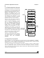
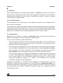
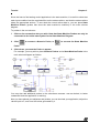
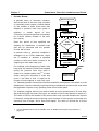
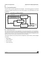
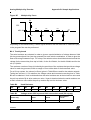
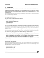
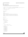
2.1 ST-Realizer Application Structures
Perhaps the best place to start describing
ST-Realizer is at the final product—the
generated assembler application that STRealizer will produce for you. It is
important to understand how the final
generated code is structured before you
start designing your application, so that
you are aware of how best to optimize
available resources, such as memory.
Reset entry point
Chip Initialization
ROS
There are two main parts to each STRealizer assembler application. The first
part is a series of initialization macros
that are embedding automatically and
that make up the Realizer Operating
System (ROS). The ROS sequentially
initializes the microcontroller, it’s I/O’s,
peripherals and memory, in much the
same way that your PC’s BIOS initializes
the PC hardware as soon as you switch Application
you create
the power on. The second part of the
code is the part that you create using STRealizer—the application program.
I/O Initialization
Peripheral
Initialization
Data memory
Initialization
Keep track of
elapsed time
Read inputs
Calculate data
Write outputs
Main
Loop
Updating of
Copies and
State Machines
Peripheral IRQs
The figure at right shows a flow chart of
the overall structure of the generated
assembler
code
that
ST-Realizer
produces.
Interrupt
Subroutines
2.2 Programming using Symbols
With ST-Realizer, you create applications by placing and connecting symbols in a scheme .
Each symbol is, in fact, a graphical representation of an assembler macro, usually including
attributes which you can modify to your specific needs.
The symbols included in the ST-Realizer main library represent a variety of coded entities
such as: mathematical, logical, conversion and power management functions, constants,
tables, subschemes/hierarchical sheets, states, input devices, output devices and sequential,
counted or time-related events.
4/248
Chapter 2
Inside ST-Realizer Applications
The symbols are made such that you need never write a single line of assembler code to
produce your application—all of the attribute modifications you may need to perform are
accessible through dialog boxes.
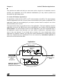
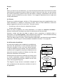
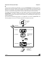
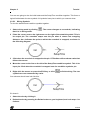
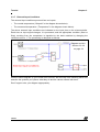
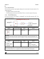
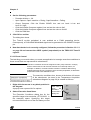
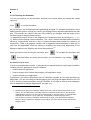
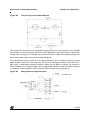
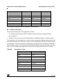
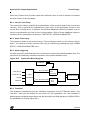
2.3 Inside ST-Realizer Applications
An application is built around an ST6 or ST7 microcontroller unit (MCU). The input signal(s)
enter the application from one (or more) of the microcontroller’s pins, ports or peripherals. The
application treats the input signal(s) as you require, and the result is output to one of the
microcontroller’s pins or ports.
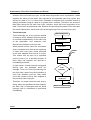
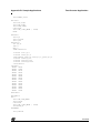
The figure below shows a generalized view of an application. The input signal(s) enter the
application via one of the MCU’s pins, ports or peripherals, and is taken up by the root (or
main) scheme. The root scheme is the core of the application—the main, sequential loop. If
the application requires any interrupts, you must create a subscheme. (Interrupts cannot
occur in the root scheme.) If you simply wish to section off a very complex part of the
application for aesthetic reasons, you may also create subschemes to contain parts of the
main loop. Subschemes are represented in the root scheme by subscheme symbols, of
which more will be said a little later.
Application
Root Scheme
Subscheme
Symbol
Table
Symbol
Input signal
Output signal
(from MCU pin,
port or
peripheral)
(to MCU pin or
port)
Additional inputs from
MCU pins, ports or
peripherals are possible.
Subscheme
5/248
Symbols
Chapter 2
2.4 Symbols
Using ST-Realizer, you design your application by placing symbols and wiring them together
in schemes.
Each symbol may represent:
• An operation, such as converting a physical analog value to a binary value,
• A piece of information related to the behavior of the application, such as a state
transition,
• A system state, or condition,
• An action reflecting a change in the system state or caused by an event such as the
occurrence of a timer interrupt.
Each symbol is associated with an ST6 or ST7 assembler code macro. The wires represent
the flow of data, and are linked to variables and constants. You can modify certain attributes
of symbols and wires, allowing you to customize them for your specific application. For
example, by attaching an attribute of type UINT (unsigned integer) to a wire, you define its
value capacity to that of an unsigned integer (0 to 65536). For more details on attributes see
Appendix A: “Variables and Attributes” on page 203.
2.4.1 State Machine Symbols
Within your root scheme, you may create a state machine, which logically guides the program
between different functional states of your application. Say, for example, you had an
application which performs the following functions:
•
Turning a motor on.
•
Setting the motor speed.
•
Turning the motor off.
In a state machine, you would define a state, using a state symbol, for each functional step
of the application above and, in addition, a state which defines the starting point of the
application—the initial state.
The sequence of state symbols would therefore look like:
•
•
•
•
Motor OFF (Initial State).
Motor ON.
Setting Speed.
Motor OFF.
The transitions between each of these states are controlled by conditions. Condition
symbols act as switches. When a condition is met, the condition symbol is triggered, and the
program can progress to the next state.
The tutorial included in this manual (see Chapter 3 “Tutorial” on page 13) provides an very
good example of how a state machine and state symbols can be used in creating an
application.
6/248
Chapter 2
Schemes
2.5 Schemes
When using ST-Realizer, you design your application in schemes. A scheme is like a plan on
which you place symbols and draw wires. Each application consists of a set of schemes,
including one root scheme and any number of subschemes. Section 7 on page 71 explains
how to build and modify schemes.
2.5.2 The Root Scheme
The root scheme is the starting point of your application program, and corresponds to the
reset vector of the program.
The root scheme is where you create the main loop of your application. All of the large scale,
sequential functions should be kept here. However, if there are any particularly complicated or
cumbersome actions in your main loop, you may wish to put them into a subscheme to save
space in the root scheme and to make the application easier to follow visually.
2.5.3 Subschemes
Applications can include any number of subschemes which contain further symbols and
wires but are displayed in the root scheme as a single symbol.
There are three reasons to create a subscheme:
•
To include complex portions of the main loop, thus saving space in the root scheme and
making it easier to reuse processes. In this case, the subscheme is executed as if it were
a part of the main loop (root scheme).
•
To include parts of the application that are event-driven. (Events can never be placed in
the root scheme.) Subschemes can be assigned either a single execution condition,
which will apply to the entire subscheme, or alternatively, can include any number of
event symbols. More will be said about execution conditions and events shortly.
•
To save functional parts of your application (analogous to subroutines) that you may wish
to reuse in other applications. Subschemes are saved in their own files (.sch files) and
can be easily copied to other ST-Realizer projects and reused. You may also save
customized subschemes symbols to a library, to be accessible by all projects.
(Subscheme symbols are described below).
Designing a subscheme is no different than designing an ordinary scheme, with one
exception: a subscheme has connections to its root scheme via a subscheme symbol. The
subscheme symbols are named sssp_q, where p indicates the number of inputs you need for
your symbol and q the number of outputs. For example, sss2_1 is a subscheme with two
inputs and one output.
7/248
Events
Chapter 2
When you want to use a subscheme, you must therefore first think about its connections: what
inputs does the subscheme need to deliver its output? Once you know this, you can choose
the correct subscheme symbol from the main library. However, subschemes, like the root
scheme, can be modified at any time. Section 7.4 on page 85 describes how to create and
modify subschemes.
2.6 Events
Events are conditional triggers, similar to If..Else statements, that can be applied either to an
entire subscheme, or simply to a sequence of code. Like an If..Else statement, events are
always triggered by an input of some sort. The input may be:
•
An interrupt, such as a timed or hardware interrupt.
•
An input value change.
When an event is applied to an entire subscheme, it is called an execution condition—
because it defines the conditions by which the subscheme will be executed.
However, events can also be made to apply to just a sequence of symbols within a
subscheme, using event symbols. These symbols act as switches—if the condition that they
represent is met, the code that follows them can be performed.
There are many types of events, some hardware independent, and others that are hardware
dependent. The full range of events available is detailed in Section 7.4 on page 85.
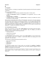
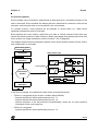
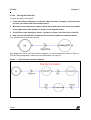
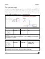
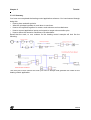
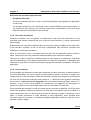
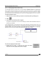
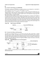
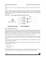
2.6.4 Execution Conditions
An execution condition can be applied to a subscheme,
such that the subscheme is only executed when that
execution condition is met—such as a timed interrupt,
or upon a subscheme input change. Only one execution
condition can be applied to any given subscheme and
when this execution condition is fulfilled, all of the code
within the subscheme is executed.
Subschemes with execution conditions are chiefly used
to contain reasonably complex subroutine functions
that are conditionally performed in addition to the code
in the main programming loop.
The diagram at right shows a schematic example of
how a subscheme with execution conditions is used in
an application.
Reset entry point
Initialization
Normal Code
Execution
Is
Execution
Condition
met?
Y
Subscheme
Code
Normal Code
Execution
8/248
N
Chapter 2
Events
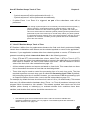
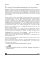
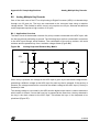
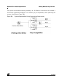
2.6.5 Event Symbols
Event symbols can be included in subschemes to determine when, and which portions of, the
code is executed. Event symbols are always placed in subschemes, because events act as
interrupts, and interrupts may never be placed in the root scheme.
In a certain manner, event symbols act as switches to control when (i.e. under which
conditions) subsequent code is executed.
Event symbols are most usefully used when you wish to include several events that may
control the similar portions of code. However, certain rules apply when placing more than one
event symbol in a single subscheme (refer to Section 7.4.5 on page 89).
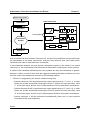
The diagram below shows a schematic example of how event symbols can be used to control
how a subscheme is executed.
Reset entry point
Subscheme Code
Initialization
symbol sequence A
Normal Code
Execution
Event 1
out1
Event 2
out2
event symbols
Subscheme
Symbol
symbol sequence B
symbol sequence C
Normal Code
Execution
In the above example, the subscheme code will be executed as follows:
•
If Event 1 is triggered (by the event’s condition being fulfilled):
- Symbol sequence A will be performed with out1 = 1.
- Symbol sequence B will be performed with out2 = 0.
- Symbol sequence C will be performed unconditionally—there are no event symbols
connected to this code sequence.
•
If Event 2 is triggered:
- Symbol sequence A will be performed with out1 = 0.
9/248
How ST-Realizer Keeps Track of Time
Chapter 2
- Symbol sequence B will be performed with out2 = 1.
- Symbol sequence C will be performed unconditionally.
•
If neither Event 1 nor Event 2 is triggered, no part of the subscheme code will be
performed.
Note:
Even though symbol sequence C is not directly connected to a event symbol, by
virtue of it being in a subscheme with that contains events, it will not be
performed unless one of the events is triggered. The golden rule is that you
cannot mix events with root scheme symbols (meaning those symbols that are
performed as part of the main loop or normal code). When you place symbols
in a subscheme which contains one or more events (either in the form of event
symbols or an execution condition), those symbols cannot be considered as
part of the root scheme.
2.7 How ST-Realizer Keeps Track of Time
ST-Realizer II differs from its predecessors because the final code that it produces will only
contain timer initialization code if there are time-related symbols or events in the application.
However, if your application includes either time-related symbols or events, ST-Realizer will
generate something called a base clock timer tick in the following manner:
•
Every ST6 and ST7 microcontroller has a timer, called Timer 1 (ST6) or Timer A (ST7),
which (if there are either time-related symbols or events in the application) is used as the
base clock to measure out units of time called “timer ticks”. You can choose to set the
value of the timer tick—this is described on page 131.
•
All time-related symbols and events are based on timer ticks. This means that one timer
tick is the smallest increment of time that can be distinguished.
•
Timer ticks may be used to control the processing time of a main loop cycle. The time
required to perform one main loop cycle is called the Processing Cycle Time. By default,
the processing cycle time is variable. However, you can choose to fix the processing cycle
at a specific number of timer ticks—how to do this is described on page 131.
For example, by default the base clock timer tick is set to 0.01 s (10 milliseconds). This means
that every 10 milliseconds the hardware timer (Timer 1 or Timer A) sends an interrupt to the
program which increments a tick variable. Time-related symbols and events use this tick
variable (either directly or indirectly(1)) to evaluate whether their conditions have been
satisfied, and whether their actions should be executed or not.
1
10/248
How different types of time-related events use the value of the tick to evaluate their
conditions is detailed in Section 7.4.3 on page 85. Time-related symbols are described in
detail in Section 8.4 on page 116.
Chapter 2
Connecting your Application to the Target Device
The concept of the base clock timer tick is an important one, because it appears every time we
require a time-related symbol or event. In our tutorial example, we demonstrate how to use
both time-related symbols and timed events. We strongly urge you to take the time to
complete the tutorial—it is a very efficient way to get up to speed in ST-Realizer and the time
you spend doing the tutorial will be saved later by having increased your productivity!
2.8 Connecting your Application to the Target Device
All signal inputs to the application are supplied by one or more of the microcontroller’s input
pins, ports or peripheral control registers. Similarly, the application’s final output must also be
sent to an output pin or a port. In general, each ST6 and ST7 microcontroller has a variety of
digital and analog input/output pins, as well as ports for serial or parallel data. The number of
pins and ports, of course, depends on the microcontroller in question.
However, peripheral support can vary largely, depending on the microcontroller to be used.
Any application design, must obviously bear in mind the resources available on the
microcontroller.
To link inputs and outputs between the application and the microcontroller, you must connect
pins, ports or peripheral control registers to input or output symbols in the application’s
schemes.
Note that peripherals must be enabled before they can be used by the application. Once
enabled, each peripheral used must usually be configured to meet the hardware requirements
of your application—hardware setting dialog boxes are designed for this purpose. These
hardware settings are used by the ROS to initialize the microcontroller properly.
2.9 Application Development Steps
Once you have designed your application using ST-Realizer, you analyse and compile it
using ST-Analyser.
ST-Analyser performs the following tasks:
•
Analyses your scheme by creating the netlist, creating cross references, analysing and
generating final code. Providing no fatal errors are encountered, ST-Analyser generates a
non-compiled ST6 or ST7 macro-assembler language (.asm) file from the scheme.
•
Generates the compiled binary ST6 or ST7 executable file. Depending on whether or not
you included the ROS (see Section 2.3 on page 5 and Section 5.3.4 on page 63), a file
with extension *.hex or *.obj respectively is generated for ST6, or with extension *.s19 or
*.obj for ST7. A *.hex (or *.s19) file can be directly loaded into an ST MCU while you
must link a *.obj file with another program.
When the analysing process has been successfully completed, a report file is generated. This
report file gives information about the designation of I/O pins, a list of the variables used by
type and the memory space required by the application.
11/248
Application Development Steps
Chapter 2
Once you have compiled your application, you can use ST-Simulator to simulate its behavior,
generate and view input signals, monitor signals that are generated by your application, and
fine-tune it if necessary. You design simulation environments in the same way you design
schemes, except that the design is held in what are called simulation environment files.
To provide you with greater flexibility, you can create or edit your own symbols using STSymbol Editor. You create a symbol by drawing its shape, placing pins that represent the
variables that are input to and output from the process you are defining, then linking it to the
macro it represents.
All the files and definitions that pertain to an application are stored in project files. The
following diagram shows the ST-Realizer application development process.
Application
Idea
Project FIle
ST-Realizer
Draw the schemes
ST-Analyser
Compile the code
and generate the
report
ST-Simulator
97
Test and debug
the code
Load the code
into an ST
microcontroller
12/248
Chapter 3
3
Tutorial
TUTORIAL
The following tutorial is designed to help you fully understand both the principles behind
creating applications using ST-Realizer and how to create applications using ST-Realizer.
In this tutorial, you’ll learn how to create an ST microcontroller application.
The application you will create manages a heating control system. The ambient temperature
is periodically measured, filtered and compared with a preset value. When the measured
temperature is lower than the control value, the heating system is started while the pump
speed is adjusted proportionally to the temperature differential. A pilot LED lights up to show
that the heating is on. When the measured temperature exceeds the control value, the heating
system is stopped.
This tutorial application runs in stand-alone mode using an ST72212G2 microcontroller.
However, note that the same application could be applied equally to an ST6 microcontroller,
such as the ST6265, with little modification. The goal of this tutorial is to demonstrate, in a
general manner, how to use ST-Realizer, rather than to supply sample applications for a given
microcontroller.
3.1 Setting Up Your Project
In this part of the tutorial you will:
•
Create a new project file for the heating control application.
•
Define the ST microcontroller onto which the application will be loaded.
•
Learn how to open the scheme in which you'll draw the application.
3.1.1 Creating the Project File
Each application you design is stored in a project. When you create a new project, the first
step is to specify the folder in which you wish to place it. It is recommended that you create a
separate folder for each new project.
ST-Realizer will creates a project.rpf file, that contains project-specific path settings, the
project's scheme names, target hardware information and compiler settings.
Once you've defined your project, you'll be able to open a new scheme and start designing
your application.
13/248
3
Tutorial
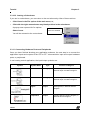
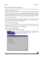
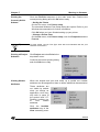
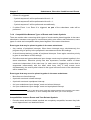
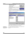
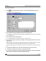
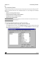
1
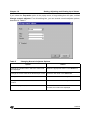
Chapter 3
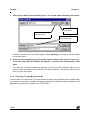
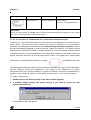
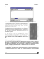
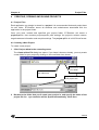
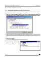
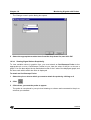
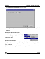
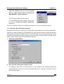
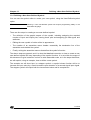
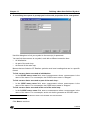
È
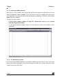
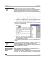
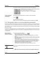
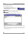
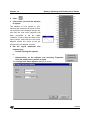
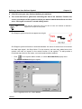
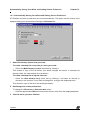
Click Project New in the cascading menu. The Create a New File dialog box opens:
Click here to create
a new folder.
Click here to move up
one folder level.
Type the name of your
new project here.
Create a new folder for your tutorial project called “Heating” by clicking on the new folder
icon shown above.
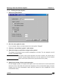
2
Once you have created your project folder, type the name of the project (“heating”)
in the File name field. ST-Realizer will add the .rpf extension automatically. Click
Save.
You have just created the heating.rpf file in which the main settings related to your
project will be recorded at the end of the ST-Realizer session. They will be used the next
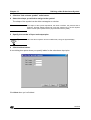
time you open the project.
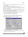
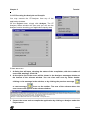
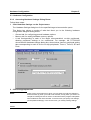
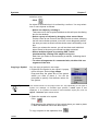
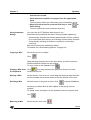
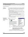
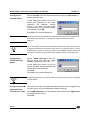
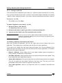
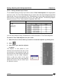
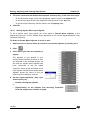
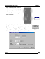
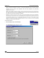
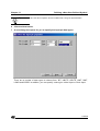
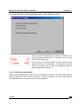
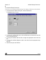
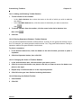
3.1.2 Choosing a Target Microcontroller
The next step is to choose the ST microcontroller on which the application will be loaded. After
you create a new project, a window will open prompting you to select the target hardware. This
application is going to be loaded on an ST72212G2:
14/248
Chapter 3
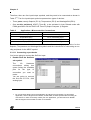
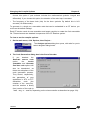
Tutorial
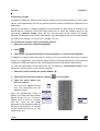
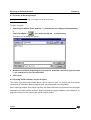
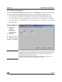
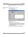
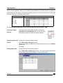
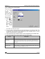
1
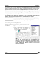
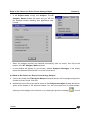
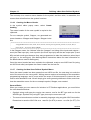
Click the Target Hardware folder in the Select Target Hardware window. A
browsable list of target hardware devices will appear in the window shown below.
2
Find the desired ST microcontroller (ST72212G2) by clicking the device icons in the
list until the name of the chosen device is displayed. Select the ST microcontroller
ST72212G2 by clicking once on it.
3
Click OK to confirm.
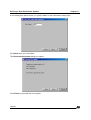
You may also double-click the line showing the device.
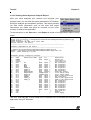
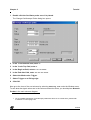
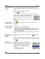
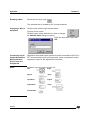
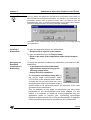
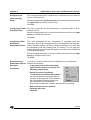
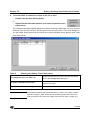
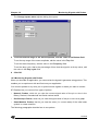
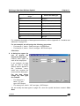
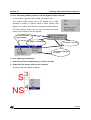
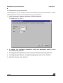
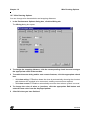
4
Once you have selected your target hardware, the Project window will open, as
shown below:
This window will list all of the components of your project—schemes, libraries and target
hardware. Notice that ST-Realizer has already created an application scheme file called
heating.sch by default. Next, we’ll learn how to design the application scheme.
15/248
Tutorial
Chapter 3
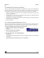
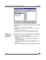
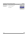
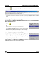
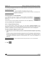
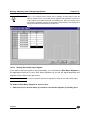
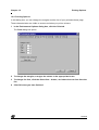
3.1.3 Opening the Main Scheme
Now that you have created your project and specified the target microcontroller, you must
draw the main (or “root”) scheme. This is the sheet on which you design the main part of
your application. The main scheme file has already been created by ST-Realizer, and is called
heating.sch by default.
To open the main scheme:
•
In the Project window (shown on page 15), double-click heating.sch, located
under the Schematics folder.
A new blank worksheet opens where you can draw the main (root) scheme of the
application:
3.1.4 The Worksheet Toolbar
At the top of the scheme worksheet, you will see a toolbar with a number of icons. How to use
these icons will be described as we work through the tutorial, but a quick summary of their
names and uses is given here.
16/248
Tutorial
N
ew
O P
pe ro
Sa n F jec
ve ol t
C F de
u ile r
C t
op
Pa y t
s o
D te Clip
el
bo
e
ar
Se te
d
le
W ct
iri To
A ng ol
na T
o
Pr lys ol
e
ev r
N iou Me
ex s s
s
C t M Me ag
ha e s e
s
s
In nge sa sag
fo P g e e
M rma ro
irr t pe
i
R or O on rtie
ot
b on s
A ate jec S of
dd O t e l A
ec ttr
C Ne bje
te ib
op w c
d ut
t
y
O e
L
O L a
bj
pe o b
ec
e
c
C n S al l t
t
op y O o
y mb bje Sc
Zo Sy o c he
m lL t
m
Zo om
bo ib
e
r
I
om n
l
ar
Pa
ie
s
n Ou
t
Fi
ti
n
H to
el
W
p
in
do
w
Chapter 3
Note:
The step-by-step instructions in this tutorial describe how to operate STRealizer using the default toolbar setup shown above. If, while you are doing this
tutorial, you cannot find a button that is shown in an instruction, refer to
“Customizing Toolbars” on page 199, to find out which menu commands
correspond to that button.
3.2 Designing and Drawing Schemes
For the heating control application, the microcontroller will require the following inputs and
outputs:
•
2 analog inputs:
- The actual temperature
- The control temperature
•
1 digital output to one pilot LED to indicate the heating system status,
•
1 digital output to control the speed of the pump.
In this part of the tutorial, you are going to learn how to create the above application by
drawing graphical schemes. In particular, you will learn:
•
How to place symbols.
•
How to edit symbols.
•
What the principal symbols do, and when to use them.
•
How to connect the pins.
•
How to handle events.
The schemes associated with the application include symbols that describe:
•
A State Machine diagram.
•
Conditions, that is conditions that are transmitted to the application from external sources
such as temperature records, or that are internally determined, for example when the
17/248
Tutorial
Chapter 3
system switches to a specific state.
•
Actions, that is actions that are output from the application, such as putting on the pilot
LED, or actions that are internally determined, for example those resulting from a timer
interrupt.
The following section will explain how to draw the heating application using symbols fulfilling
the above roles.
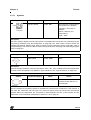
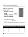
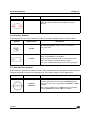
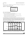
3.2.5 The State Machine Diagram
Each time a condition changes, as a result of the signals received from the microcontroller
input pins, the state machine selects the appropriate state. The state defines the signals that
are sent to the microcontroller output pins.
The overall management of the heating control system is carried out by a simple state
machine with four states: Init, HeatingOFF, HeatingON, and Pump Enabled.
SetupTime, Start, SetPump and Stop conditions trigger state transitions.
A specific action is associated with each state.
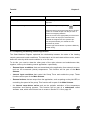
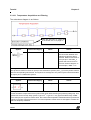
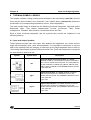
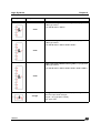
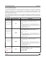
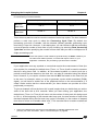
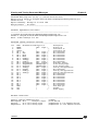
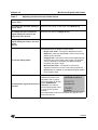
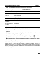
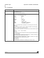
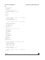
The following table summarizes the relationship between events(1) (or inputs), conditions and
actions.
Event(1) or Input Signal
Internal
External
Event = Timer
Interrupt
1
18/248
Action
Condition
New State
SetupTime
HeatingOFF
Pilot LED OFF
Measured Temp.
is lower than
Control Temp.
Start
HeatingON
Pilot LED ON
Measured Temp.
exceeds Control
Temp.
Stop
HeatingOFF
Pilot LED OFF
SetPump
PumpEnabled
Pump speed
control active
Setup Time has
elapsed
System switches
to HeatingON
state
State Transition
No state transition
For more information about Events, please refer to Section 7.4 on page 85.
Input acquisition
active
Chapter 3
Tutorial
When you define the state machine, the first symbol you must place is the initial state.
For the heating control application, the initial state is Init. This is a holding state that allows
time for the application to measure and filter the actual temperature, before deciding whether
to turn on the heat pump.
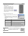
3.2.5.1
Placing the Initial State
To place the initial state, Init:
1
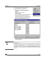
Click
.
2
The main library dialog box will open, as shown at right:
All of the symbol names are categorized by function. A
complete listing of symbols (organized by functional category
and name) can be found in Chapter 8 on page 103.
The initial state symbol is called “stateinit”, located under the
“State machine” category.
Find “stateinit” and select it by:
•
double-clicking on it,
or,
•
3
clicking once on it and, without moving the cursor
from the library dialog box, right-click the mouse and select Place.
A square box will now appear next to the cursor, indicating the size and position of
the “stateinit” symbol. Move the cursor to where you want to place the symbol, then
click once. It is recommended that you place the symbol towards the top and left of
your scheme.
Note:
4
If you wish to move the symbol after having placed it, just click once next to the
symbol so that a red rectangle appears around the entire symbol, indicating that
it has been selected. Then simply drag and drop it where you wish.
A dialog box will open, prompting you to edit the value of the state. In doing so, you
are effectively naming the initial state variable. Type “Init” in the field, then click
OK.
CAUTION:
With ST-Realizer, object naming (such as when you assigned the name “Init” to
the initial state symbol above) is case-sensitive. In addition, spaces are interpreted as characters. Ensure that all object names are used consistently, otherwise, errors will result when you compile the application.
19/248
Tutorial
Chapter 3
You've just placed your first symbol—the initial state, Init. It should look like this:
If it doesn't, select the symbol by clicking next to it, then delete it by pressing the Delete button
on your keyboard, and redo steps 2 to 4 above.
If you find that the symbol is too small, and you want to zoom in on it, click
, then select
the area around your symbol. If you make a mistake, and can no longer see your symbol, click
to see the whole scheme, then reuse
to zoom in on your symbol.
Now you are ready to place the first condition—the SetupTime condition—that is activated for
the first time when the start button is pressed. Active conditions are signalled by sending the
value 1—a signal value equal to 0 indicates that the condition is not active.
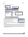
3.2.5.2
Placing a Condition
To place the Start condition:
1
In the main library dialog box, under the category “State machine”, scroll down the
list until you find “condition”, then double-click it.
2
Move the cursor to where you want to place the symbol (i.e. to the right of the
stateinit symbol as shown in the diagram below), then click.
3
The Edit the value dialog box opens. Type “SetupTime” in the field, then click OK.
Your scheme should now look like this:
If it doesn’t, select the incorrect symbol by clicking next to it, then delete it by pressing the
Delete button on your keyboard, and redo steps 1 to 3 above.
20/248
Chapter 3
Tutorial
You are now going to wire the initial state and the SetupTime condition together. This forms a
logical link between the two symbols. All symbols have pins to which you connect wires.
3.2.5.3
Wiring Symbols
To wire the stateinit and condition symbols together:
1
Select wiring mode by clicking
that it is in wiring mode.
. The cursor changes to a crosshair, indicating
2
Place the cursor next to the right arrow on the right of the stateinit symbol. This is
its output pin. The crosshair snaps onto the pin when it comes into snapping
distance. An x indicates the point to which the crosshair is snapped, as shown in
the following diagram:
3
Click when the crosshair is snapped to the pin. ST-Realizer will now draw a wire that
follows the cursor.
4
Move the cursor to the line on the left of the SetupTime condition symbol. This is its
input pin. Click when the crosshair is snapped onto the condition symbol’s pin.
5
Right-click the mouse or press the ESC key or click
symbols are now connected by a wire.
to finish wiring. The two
Your scheme should now look like this:
If it doesn’t:
1
Select the wire by clicking it.
2
Delete the wire by pressing the Delete button on your keyboard, and redo steps 1 to
6 above.
21/248
Tutorial
3.2.5.4
Chapter 3
Placing the Next State
To place the state, HeatingOFF:
1
In the main library dialog box, under the “State machine” category, scroll down the
list until you reach state, then double-click it.
2
Move the cursor to where you want to place the symbol, then click. Place the symbol
to the right of the state symbol, as shown in the diagram below.
3
The Edit the value dialog box opens. Type HeatingOFF in the field, then click OK.
4
Now, wire the SetupTime condition to the new state symbol as explained above.
Your scheme should now look like this
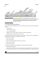
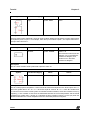
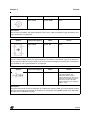
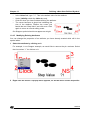
Now design the rest of the state machine diagram, so that it appears as shown in Figure 1.
The following paragraphs contain hints and explanations to help you.
Figure 1 The final state machine diagram.
22/248
Chapter 3
3.2.5.5
Tutorial
Designing the Complete State Machine Diagram—Hints and Explanations
Reminder: The application manages a heating control system. The ambient temperature is
periodically measured, filtered and compared with a preset value. When the measured
temperature is lower than the control value the heating system is (re)started while the pump
speed is adjusted proportionally to the temperature differential. A pilot LED lights up to show
that the heating is on. When the measured temperature exceeds the control value, the heating
system is stopped.
When the application is started, the initial state, Init, triggers a counter that allows enough time
for the system to measure and filter the actual temperature value. Once this time has elapsed,
the SetupTime condition is met, and triggers the HeatingOFF state, while simultaneously
evaluating the temperature inputs. If the temperature differential between the actual
temperature and the setpoint temperature is larger than a preset constant, a new condition
called Start is met and a signal equal to 1 is sent. This signal triggers the transition between
the HeatingOFF state and the HeatingON state, meaning that the heating system is powered
and the pilot LED is switched on. To create the HeatingON state we must place a state
symbol, to which we assign the name value HeatingON, and then wire it to the Start
condition, as shown in Figure 1.
Now, the pump should operate in such a way that its speed is proportional to the differential
observed between the actual temperature value and a preset temperature value. In order to
do this, the pump must be enabled prior to operation. The system must change to the
PumpEnabled state. A new condition symbol, SetPump, is needed, that will trigger the
transition between the HeatingON state and the PumpEnabled state.
Similarly, another condition, Stop, will ensure the transition between the PumpEnabled state
and the HeatingOFF state.
You can see that the same symbol (“condition”) is to be used four times (the “state” symbol
itself is to be used three times).
When one symbol already exists in a scheme, you can copy it rather than selecting it from the
library. Since you are now going to place the Start condition symbol, you can copy it from the
SetupTime condition symbol:
1
Click just next to the SetupTime condition symbol to select it.
2
Click
3
Click where you want to place the copy (beside the HeatingOFF state symbol, as
shown in Figure 1).
.
23/248
Tutorial
Chapter 3
4
Double-click the name of the symbol. The Edit the value dialog box opens. Type
Start, the name of the new condition, then click OK.
5
For the HeatingON state symbol, select and copy the HeatingOFF state symbol
using
. Place it beside the Start condition symbol. Double-click the name of
the symbol and enter the new value HeatingON, as shown in the diagram.
6
Create the SetPump condition in the same manner that you created the Start
condition. Note that in the State Machine diagram, the SetPump condition symbol is
in the opposite direction to the Start condition symbol. You can change its direction
using the mirror function, by clicking on
position by clicking
7
, or by rotating it to the required
twice.
For the PumpEnabled state symbol, select and copy the HeatingON state symbol
using
. Place it at the bottom of the State Machine diagram. Double-click the
name of the symbol and enter the new value PumpEnabled, as shown in the
diagram.
8
For the Stop condition symbol, select the select the SetPump condition symbol,
click
to copy it, place the new symbol at the left of the PumpEnabled state
symbol, then enter the value Stop.
The next step is to wire the HeatingON state symbol, the three new condition symbols and the
PumpEnabled state symbol. Look at the state machine diagram to see how these are wired
together.
In your scheme, make sure wiring mode is selected by clicking
Note:
24/248
and wire the symbols.
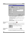
Auto wiring and Auto reroute are options available in the
Option Environment Wiring menu path. These options create corners and
reroute wires across the shortest path automatically. If you prefer to connect the
wires another way, you can deactivate them:
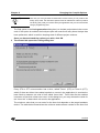
1 On the Options menu, select Environment.
2 In the Environment Options dialog box click the Wiring tab.
3 Click the Auto wiring and Auto reroute check boxes. When these are empty,
Auto wiring and Auto reroute are deselected.
È
È
Chapter 3
Tutorial
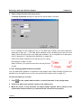
To place a heading in the diagram:
1
Click anywhere in the diagram area with the right mouse button.
A popup menu displays.
2
Select the New/Attribute options
The Create an Attribute dialog box opens.
3
Specify the following options:
TAG = TXT,
Value = “State Machine Diagram” (enter text)
Visibility = Tag checkbox left unchecked
4
Place the heading where you want, by dragging it
5
Click OK.
You’ve just drawn the state machine, which is part of the main scheme of the heating control
application.
The next section will explain how to draw the rest of the heating control application. Since you
should now be used to placing, editing and wiring symbols, the descriptions that follow will
explain what symbols you will place, with what values and why the symbols are there. They
will not include details on how to place, edit and wire the symbols that are there. Table 2
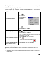
shows a summary of the editing functions that you can use to create the remaining diagrams.
Table 2
Summary of Editing Functions
To do this:
Select a symbol
Do this:
Choose the select mode by clicking
toolbar.
on the
Keeping the left mouse button pressed, drag a box
around the symbol, or click near the symbol with
the left mouse button.
Move a symbol
Select the symbol then drag-and-drop it where you
want to place it.
Copy a symbol
Select the symbol. Click
on the toolbar.
Click where you want to place the copy.
Change the name of a symbol
Double-click the name that is currently displayed
with the symbol. The Edit the Value dialog box
opens. Type the new name. Click OK.
25/248
Tutorial
Chapter 3
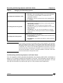
To do this:
Do this:
Delete a symbol
Select the object. Press the Delete key on your
keyboard.
Wire two symbols together
Select the wiring mode by clicking
.
Place the cursor next to the output pin on the first
symbol. A crosshair snaps onto the pin when it
comes into snapping distance.
Move the cursor to the appropriate pin of the other
symbol. This is an input pin. Click when the
crosshair is snapped onto the symbol’s pin.
The two places where you clicked are now
connected by a wire.
Click the right mouse button or press the ESC key
to finish wiring.
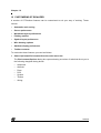
3.3 Completing the Heating Control Application
The State Machine Diagram explained the relationship between the state of the heating
control system and certain conditions. The next step is to link each state with an action, and to
define the rules by which each condition is, or is not, met.
To do this, you need to draw the other parts of the main scheme and subschemes that,
together, make up the heating control application—specifically:
•
External Input conditions, that are transmitted to the application from external sources,
such as the measured (actual) temperature. This function will be part of the Main
Scheme.
•
Internal input conditions that control the Setup Timer and enable the pump. These
functions will be part of the Main Scheme.
•
External actions, that are output from the application, such as putting on the pilot LED, or
controlling the speed of the pump. This function will be part of the Main Scheme.
•
An internal event-driven action such as the periodic activation of the temperature
acquisition and filtering process. This function will be part of a subscheme called
filter.sch, which we will learn how to create in Section 3.3.10 on page 35.
26/248
Chapter 3
Tutorial
3.3.6 What differentiates a main scheme from a subscheme?
Each diagram (meaning a collection of symbols wired together) in a scheme is analogous to a
sub-routine in a program. The main scheme is, if you will, the conceptual core of your
application. It pays to keep things simple in the main scheme, and to only include diagrams
that represent the large-scale, sequential running of the application.
All of the highly detailed acquisition, filtering and comparison programs are better put into
subschemes so that the application will be easier to de-bug or update later.
There are two good guidelines to keep in mind when deciding when to put something into a
subscheme, rather than in the main scheme:
•
Size and complexity of the diagram - the larger and more complex the diagram, the more
reason to put it into a subscheme by itself,
•
If the function that the diagram performs runs in parallel to other functions (for example, a
sampling program that periodically reads external inputs continuously), it must be put in
a subscheme.
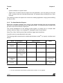
The entire main scheme of the heating control application is shown below. Only one
subscheme—for the internal event-driven action described above—will be created after we
finish the main scheme.
We have already completed the State Machine Diagram (top left). The remainder of the main
scheme diagrams are described in the following paragraphs.
27/248
Tutorial
Chapter 3
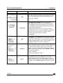
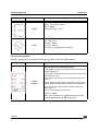
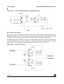
3.3.7 External Input Conditions
The external input conditions proceed from two inputs:
•
The control temperature (“Setpoint” in the diagram shown below).
•
The measured temperature (“Temperature” in the diagram shown below).
The above external input conditions are indicated on the input pins on the microcontroller.
Each time an input signal changes, it is processed, and the appropriate condition (Start or
Stop) resulting from the comparison is signalled to the state machine by changing the
condition value to 1. The processing is designed as follows:
Diagram cont’d in
Section 3.3.9.2
on page 34
Draw the above diagram on your heater main scheme, with the help of the following tables that
describe the symbols you’ll place, what they do and the values entered with them.
Don’t forget to wire your diagram appropriately.
28/248
Chapter 3
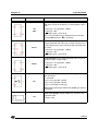
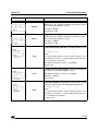
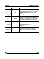
3.3.7.1
Tutorial
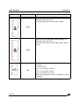
Symbols
Symbol
Functional Category
Input and output
Name
Symbol: adc
Values
There are two occurrences of
this symbol in the diagram:
Comment = As shown in
diagram
Name = SetPoint and
Temperature.
Type = UINT
Description
This is an analog to digital converter input symbol. The NAME value connects it to a hardware port (see
“Connecting Hardware Ports and Peripherals” on page 38). The TYPE value is used to define the
variable type (UBYTE, SBYTE, UINT, SINT or LONG). The two instances have the Type UINT, which is
unsigned integer. The comment value is used in the report file (see “Analysing and Generating Program
Code” on page 44).
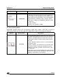
Symbol
Functional Category
Mathematical
Name
Symbol: sub2
Values
None
Description
This is a two input subtractor, with type inheritance. OUT = IN1 - IN2. It subtracts the actual temperature
from the Control Temperature. For details on type inheritance, see “Type Inheritance” on page 204.
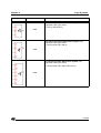
Symbol
Functional Category
Hierarchical Sheet
Name
Symbol: sss1_1
Values
Scheme = Name of the related
subscheme file (filter.sch, in
the example).
Description
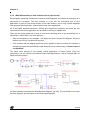
This is a subscheme connection symbol. It represents a process that is contained in a sub-scheme. In
this case, the subscheme has one input (“In”) and one output (“Out”). By using Portin and Portout
symbols within the subscheme the connection is made between the pins of this symbol and the
subscheme. This subscheme is described in Section 3.3.10 on page 35.
29/248
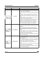
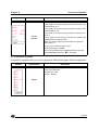
Tutorial
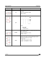
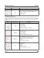
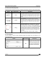
Symbol
Chapter 3
Functional Category
Logic
Name
Symbol: mux1
Values
None.
Description
This is a single-output multiplexer, where an input condition determines whether the output value should
be equal to input 0 or input 1. For example, when the input condition equals 1, the output value will be
the input value from line 1.
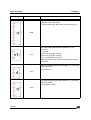
Symbol
Functional Category
Constant
Name
Symbol: constw
Values
Value = 10
There are two instances in this
diagram, one in the ARTimer
subscheme diagram, and
another one in the Filter
subscheme diagram.
Description
This is a word constant value symbol that inputs the value 10.
Symbol
Functional Category
Conversion
Name
Symbol: comp
Values
None
Description
This is a multi purpose comparator. It returns three bit values that depend on the three inputs. B>A = 1
when B is greater than A. B = A = C = 1 when B is equal to A and C. B < C = 1 when B is smaller than
C. There is one occurrence of this symbol. It indicates the Start condition, when this condition is met, by
outputting 1. This condition is met when the differential between the control temperature and the actual
temperature is greater than 1 degree C. It indicates the Stop condition (output=1 on this pin) when the
differential between the control temperature and the actual temperature is negative.
30/248
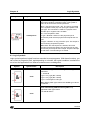
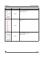
Chapter 3
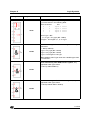
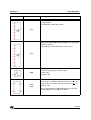
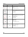
Symbol
Tutorial
Functional Category
State machine
Name
Symbol: stateout
Values
Name = HeatingON
Several additional
occurrences of this symbol
can be found in other main
scheme diagrams.
Description
This is an example of a state output symbol. State output symbols are connected to state symbols by
their names. When the system switches to the specified state, the processing that follow the state output
symbol is performed. In the example, the processing simply consists of enabling the pump.
Symbol
Functional Category
State machine
Name
Symbol: statein
Values
There are two occurrences of
this symbol in this diagram:
Name = Start
Name = Stop
Another instance of this
symbol can be found in the
Internal Input Condition
diagram.
Description
These are state input symbols, that connect to condition symbols in the state machine that have the
same name. For example, when the bit value 1 is received from the B>A output of the comparator, it
signals the Start condition by outputting the value 1 to the state machine.
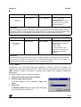
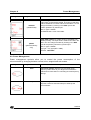
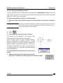
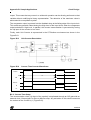
3.3.7.2 Wires
Occasionally, you must attach data type attributes to wires to control the outputs. For
example, you must attach attribute TYPE = SINT to the wire connected to the output pin of the
sub2 symbol in order to be able to evaluate both positive and negative temperature
differentials.
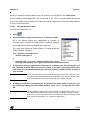
To attach a type to a wire, proceed as follows:
1
2
Click the wire with the left mouse button.
Click the right mouse button.
3
A list box displays, with 3 attributes: Type, Init,
Label.
Click Type.
The Edit the value dialog box opens, with a scrolling
list of data types to choose from.
31/248
Tutorial
4
Chapter 3
Select the type, SINT, and click OK.
SINT, stands for Signed Integer.
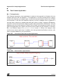
3.3.8 Internal Input Conditions
There are two internal input conditions that must be met:
•
Enough time must pass to allow temperature values to be acquired and filtered before the
temperature differential is measured. When this has happened, the SetupTime condition
is met.
•
Once the HeatingOn state is active, the pump must be enabled prior to being put into
operation by activating the SetPump condition.
The diagram is shown below:
Symbol
Functional Category
Time related
Name
Symbol: timf
Values
Name = Timer
Time = 0.05
Comment = Setup Timer
Description
This is a simple timer. The output signal is 1 until the time specified has elapsed, and then the output
becomes 0. This symbol allows enough time for the application to acquire and filter temperature values.
Symbol
Functional Category
Logic
Name
Symbol: inv
Values
None.
This symbol also occurs later
in the application.
Description
This is a multi-type bit-wise inverter. The 0 output from the timer is reverted to 1, triggering the SetupTime
condition
32/248
Chapter 3
Tutorial
3.3.9 External Actions
External actions generate output signals relating to the current state in the state machine. The
output signals are:
•
The signal to switch on the Pilot LED.
•
A PWM signal generated by the Auto-Reload Timer to control the speed of the pump.
3.3.9.1
Pilot LED Monitoring
As long as the state of the system is HeatingOFF, the Pilot LED should be OFF. The
corresponding diagram is:
Symbol
Functional Category
Logic
Name
Symbol: or2
Values
None.
Description
This is a two-value binary OR function symbol with type inheritance. If either the HeatingOFF or Init
states are active, the Pilot LED will be remain off. However, if neither of these states is active, the LED
will be ON.
Symbol
Functional Category
Input and output
Name
Symbol: digout
Values
Only one instance in the
example:
Name = HeatingIsON
Comment = Pilot LED ON
Description
This is a digital output symbol. The name value is used for connecting this symbol to the microcontroller
output ports (see Section 3.3.11 on page 38). The Comment value is used in the report file.
33/248
Tutorial
3.3.9.2
Chapter 3
Pump Speed Control
A Pulse Width Modulation (PWM) signal generated on the OCMP1_B output pin (TBOC1LR
Timer B port, for the ST72212G2) ensures pump speed control. For this, the ARCP compare
register is loaded with a value between 0 and 255 that reflects the temperature differential
calculated by comparing actual and control temperature inputs (see the “external input
conditions” diagram above).
The pump speed control diagram in the main scheme is as follows:
Cont’d from Section
3.3.7 on page 28
Symbol
Functional Category
Mathematical
Name
Symbol: mul
Values
None.
Description
This is a 2-input multiplier symbol with type inheritance. Z=A*B. Type for A and B can be any type from
UBYTE through LONG. Type for Z is the largest of A or B types. For details on type inheritance, see
“Type Inheritance” on page 204.
Symbol
Functional Category
Mathematical
Name
Symbol: limf
Values
ValueTop = 255
ValueBottom = 0
Description
This is a fixed-value limiter symbol. The output will not be larger than the top value and not smaller than
the bottom value. Type of O = type of I = any type from UBYTE through LONG.
34/248
Chapter 3
Symbol
Tutorial
Functional Category
Input and output
Name
Values
Symbol: outputlatch Name = ARCP
Comment = PumpSpeedControl
Description
This is an output symbol. The NAME value connects it to a hardware port (see Section 3.3.11 on page
38). Any type from BIT through LONG can be used.
3.3.10 The Creation of a Subscheme for an Internal Event-Driven Action
In Section 3.3.7, we made reference in the main scheme to a subscheme for an internal eventdriven action. This particular action controls the periodic activation of the temperature
acquisition and filtering process and reflects a timed interrupt execution condition—that is,
an event periodically triggered by a timer interrupt. Recall from Section 3.3.6 that all events
that need to be executed in parallel, or independently from, the main scheme, must be placed
in subschemes. In our tutorial application, the subscheme attached to this action (filter.sch )
groups code that executes as an interrupt service routine. This single-input, single-output
subscheme is represented by the sss1_1 symbol
, embedded in the main
scheme diagram where the input pin of the symbol corresponds to the input in the subscheme,
and the symbol’s output pin corresponds to the output of the subscheme. Of course,
subschemes can have various numbers of inputs and outputs, and can be represented by
symbols of type “sssx_y”, where x = the number of inputs and y = the number of outputs.
To create a subscheme:
1
Double-click on the above symbol in the main scheme diagram.
2
A window (shown below) will appear asking if you wish to create the new
subscheme. Click OK.
A new blank scheme will appear.
35/248
Tutorial
Chapter 3
3.3.10.1 Temperature Acquisition and Filtering
The subscheme diagram is as follows:
Note: We will learn to create this
box in Section 3.3.12 on page 41.
Symbol
Functional Category
Hierarchical sheet
Name
Symbol: portin
Values
Label = identifier used to make
the connection between this
subscheme and the parent
scheme. Must be the name of
the input pin in the sss 1_1
symbol that can be found in
the main scheme diagram. In
the example, LABEL = “In”.
Description
This symbol is used to connect an input pin of a subscheme symbol (“sssx_y”) from the parent scheme
with the corresponding subscheme. This symbol is homologous to the portout symbol which describes
an output pin in a subscheme symbol.
Symbol
Functional Category
Logic
Name
Symbol: loopdel
Values
None.
Description
In other words the output value of this symbol is the value obtained during the previous polling loop. This
symbol acts as a one-loop delay symbol. Type of Z-1 = type of Z = any type from BIT through LONG.
In the example, this symbol is used 4 times: this means that temperature measurements are performed
5 times, one polling loop after the other. The five temperature values are then averaged to smooth the
effect of temporary variations.
36/248
Chapter 3
Symbol
Tutorial
Functional Category
Mathematical
Name
Symbol: add2
Values
None
Description
This is a two input adder, with type inheritance. OUT = IN1 + IN2. For details on type inheritance, see
“Type Inheritance” on page 204.
Symbol
Functional Category
Mathematical
Name
Symbol: div
Values
None.
Description
This is a 2-input divider symbol with type inheritance. Q = A/B, R = A modulo B. Type for A and B can
be any type from UBYTE through LONG. Type for Q and R is the largest of A or B types. For details on
type inheritance, see “Type Inheritance” on page 204.
Symbol
Functional Category
Hierarchical sheet
Name
Symbol: portout
Values
Label = identifier used to make the
connection between this
subscheme and the parent
scheme. Must be the name of the
output pin in the sss1_1 symbol
that can be found in the main
scheme diagram. In the example,
LABEL= “Out”.
Description
This symbol is used to connect an output pin of a subscheme symbol (“sssx_y”) from the parent scheme
with the corresponding subscheme. This symbol is homologous to the portin symbol which describes
an input pin in a subscheme symbol.
37/248
Tutorial
Chapter 3
3.3.10.2 Leaving a Subscheme
If you are in a subscheme, you can return to the root scheme by either of these actions:
•
Click Close in the File option of the main menu, or,
•
Click with the right mouse button any blank position in the subscheme.
A popup menu opens with five options.
Click here to return
to the root scheme
Select Leave.
You will be returned to the root scheme.
3.3.11 Connecting Hardware Ports and Peripherals
Once you have finished drawing your application schemes, the next step is to connect the
application inputs and outputs to the ST6 or ST7 microcontroller input and output hardware
ports, or peripherals.
In our heating control application, the input/output symbols are:
Symbol
38/248
Symbol Name
Type
Function in Diagram
adc
Analog Input
Control temperature acquisition, in
External Input Conditions diagram.
adc
Analog Input
Actual temperature acquisition, in
External Input Conditions diagram.
digout
Output
HeatingIsON, in External Actions
diagram.
outputlatch
Output
Loading ARCP Compare Register, in
External Actions diagram.
Chapter 3
Tutorial
Therefore, there are four input/output symbols, and they need to be connected as shown in
Table 3(1). The four input/output symbols represent two types of devices:
•
Three ports, namely Setpoint (PC.4), Temperature (PC.5) and HeatingIsON (PB.0).
•
One on-chip peripheral, ARCP (Timer B), to be activated in Auto Reload mode with
PWM generation via the TBOC1LR Timer B (Output Compare 1) Register.
Table 3
Application—Microcontroller Connections.
Application Symbol:
Microcontroller Pin:
SetPoint (adc)
PC.4, 8-bit analog input
Temperature (adc)
PC.5, 8-bit analog input
HeatingIsON (digout)
PB.0, Push-pull output
ARCP (outputlatch)
TBOC1LR Timer B Register
To make these connections, follow the instructions for connecting a port device for the
Setpoint, Temperature and HeatingIsON symbols and the instructions for connecting an onchip peripheral for the ARCP symbol.
3.3.11.1 Connecting a port device
You’re now going to connect the SetPoint input:
1
Double-click the SetPoint
adc symbol.
The
I/O
Hardware
connections dialog box
opens listing the available
pins for the type of
connection you want to
make:
You are going to connect
the first adc to PC.4, 8-bit
analog input.
1
Pin connections depend upon the application and target microcontroller. For this tutorial
application, and our target microcontroller, ST72212G2, we have specified the necessary pin
connections. In order to correctly create your own application, you will need to be familiar
with the target microcontroller for which it is intended.
39/248
Tutorial
2
Chapter 3
In the Available resources list, double-click the entry PC.4,8-bit analog input
and then click OK.
Now connect the Temperature and HeatingIsON inputs in the same way.
When you connect port devices, the dialog boxes automatically display input or output pins
depending on the type of symbol. There is no need for you to configure the ports as input or
output, prior to connecting them.
However, for on-chip peripherals, such as the Timer B on the ST72212G2, you need to
specify some hardware settings before the appropriate resource appears in the dialog box.
For instructions on how to specify these settings, see below.
3.3.11.2 Connecting and Specifying Hardware Settings for an On-Chip Peripheral
To connect the on-chip peripheral, Timer B, proceed as follows:
1
Click the Hardware Settings entry in the Project menu.
or:
Click the Properties button in the I/O Hardware connections dialog box.
2
In the Hardware settings dialog box, click the Timer B tab.
The Timer B dialog box opens.
3
At the top of the Timer B Dialog box, click the Enable box.
This action permits the application use of the Timer B peripheral and allows access to the
interrupts and control registers of the peripheral.
40/248
Chapter 3
4
Set the following parameters:
•
•
•
•
•
•
5
Tutorial
Prescaler division = 1/8.
Input Capture: Capt1 transition = Rising, Capt2 transition = Falling.
Output Compare: Click the Enable OCMP1 box and set Level 1 = Low and
Level 2 = High.
Click the Initialise Compare register1 box and set the value to 0x0.
Click the Initialise Compare register2 box and set the value to 0x100.
Click the PWM box.
Click OK to confirm.
The dialog box closes.
The Timer B on-chip peripheral is now enabled as a PWM generating device.
Consequently, a Pulse-Width Modulated signal can be generated on the OCMP1 B output
pin.
6
Now that the device is correctly configured, follow the procedure in Section 3.3.11.1
on page 39 and connect the ARCP symbol (outputlatch) to the TBOC1LR Timer B
register.
3.3.12 Event Control
The last thing you must do when you create an application is to assign execution conditions to
those events that are represented in subschemes.
Note:
Execution conditions cannot be assigned to main (root) schemes—it simply
doesn’t make sense to use the main scheme as an interrupt routine, for
example. In addition, it is best to define execution conditions after having
enabled (see page 40) any necessary microcontroller peripherals, so that these
peripheral functions are available for use.
The execution conditions box, shown at the bottom left corner
of the subscheme, (as seen in the Temperature Acquisition
subscheme diagram on page 36) is created as follows:
1
Right-click the mouse in any blank position in
the diagram.
A popup menu opens with five options.
2
Select Execution Conditions.
The Execution Conditions dialog box for the
specified target microcontroller (ST72212G2, in
the example) opens. Specifying this target
microcontroller was one of the first tasks you had
Click here to
open
the
Hardware
Connections
dialog box.
41/248
Tutorial
Chapter 3
to perform (see Section 3.1.2 on page 14).
This is the device you
have specified at the
beginning.
Name of the file where the
subscheme is saved.
Select the subscheme execution
condition (Timed Interrupt in the
tutorial example).
3
In the Execution Conditions dialog box (see above),
double-click the Timed Interrupt line.
A new dialog box opens for you to specify the time period
between input value acquisitions.
4
Enter 0.01 (1/100 second) and click OK.
5
Click the OK button in the Execution Conditions
dialog box.
6
The Timed Interrupt event is now connected to the subscheme, with a time value of 0.01
seconds. What does this mean? It means that the code described by the Temperature
Acquisition and Filtering subscheme will be executed every 1/100 of a second, after the
main processing loop has been interrupted on a priority basis. The polling of the
temperature capture points and the consolidation of the measured temperatures will thus
be performed every 0.01 seconds.
42/248
Chapter 3
Tutorial
3.3.13 Summary
You have now completed the heating control application schemes. You have learned through
doing this:
• How to place and edit symbols.
• What the principal symbols do, and when to use them.
• How to wire symbols together to create a main scheme and a subscheme.
• How to connect application inputs and outputs to target microcontroller pins.
• How to define the execution conditions of a subscheme.
Recall that the main, or root, scheme for the heating control example will look like the
following:
The next part of this tutorial will show you how to analyse and generate the code for the
heating control application.
43/248
Tutorial
Chapter 3
3.4 Analysing and Generating Program Code
In this part of the tutorial you are going to learn how to analyse the schemes you draw and
generate the program code for them.
When you execute the analysis and compile, ST-Realizer analyses your scheme by creating
the netlist, creating cross references, analysing and generating final code. During these
phases the connectivity between symbols, the I/O assignment and variable types are checked
before generating the source code. Providing no fatal errors are encountered, ST-Realizer
generates a non-compiled ST6 or ST7 macro-assembler language (.asm) file from the
scheme, which it then compiles.
When the analysing process has been successfully completed, a report file is generated. This
report file gives information about the designation of I/O pins, a list of the variables used by
type and the memory space required by the application.
3.4.14 Setting the Compile Options
There are a number of compile options that you may set before performing an Analysis of your
application. These options are discussed in detail in Section 9.2 on page 129. However, most
of the default settings are suitable for our tutorial application.
To view or set the compile options:
1
On the main menu, click Options, then Project...
The Code Generation dialog box in the Analyse Options
window opens. The default settings are suitable for our
tutorial application. Click OK.
44/248
Chapter 3
Tutorial
3.4.15 Executing the Analysis and Compile
You may execute the ST-Analyser from any of the
application windows.
On the Project menu, simply click Analyse. The ST
Analyser Status window will open and you will see the
Analyse function checking your application step-by-step.
If there are errors:
1
A dialog box will open, showing the status of the compilation, with the number of
errors and warnings. Click OK.
2
A descriptive list of the errors will be shown in the Analyzer messages window at
the bottom of the scheme window. You can view each error by either doubleclicking on its message in the window, or by clicking the previous message
or next message
icons on the toolbar. The area of the scheme where the
error occurs will appear in the scheme window.
3
Correct the errors and re-compile the application by clicking on Analyse under the
Project menu.
45/248
Tutorial
Chapter 3
3.4.16 Viewing the Analyse and Compile Report
Once you have analysed your scheme and compiled your
program code, you can view the report generated by ST-Realizer
during the analysis and compilation process. This report provides
you with useful information such as the input and output
connections you made, and gives an overview of how much
memory is used by the application.
To see the report, on the View menu, click Report. A portion of our application report is shown
below:
ST72212G2 Realizing Unit (V4.00) (c) 1990-98 Actum Solutions
Report file of project C:\Program Files\ST-Realizer\Examples\Heating\heating.rpf
Scheme Version
: 1.00
Report timestamp: Wed Apr 14 13:14:40 1999
Analyze results : No errors
------------------------------------------------------------------Schematic dependencies and events:
------------------------------------------------------------------C:\Program Files\ST-Realizer\Examples\Heating\heating.sch
Scheme: C:\Program Files\ST-Realizer\Examples\Heating\Filter.sch
Event: Timed interrupt 0.01 Sec.
ST72212G2 (DIL28) connection overview:
------------------------------------------------------------------Pin
Name
Alternative name
Type
I/O
Description
1:
RESET
(BIT
Input ),
Active low
2:
OSCin
),
Oscillator In
3:
OSCout
(
),
Oscillator Out
4:
PB.7
SS
(BIT
Input ),
Not connected
5:
PB.6
SCK
(BIT
Input ),
Not connected
6:
PB.5
MISO
(BIT
Input ),
Not connected
7:
PB.4
MOSI
(BIT
Input ),
Not connected
8:
PB.3
OCMP2_A
(BIT
Input ),
Not connected
9:
PB.2
ICAP2_A
(BIT
Input ),
Not connected
10:
PB.1
OCMP1_A
(BIT
Input ),
Not connected
11:
PB.0
HeatingIsON
(BIT
Output),
Push-pull output
12:
PC.5
Temperature
(UBYTE Input ),
8 bit analog input
13:
PC.4
Setpoint
(UBYTE Input ),
8 bit analog input
14:
PC.3
ICAP2_B
(BIT
Input ),
Used by the application
15:
PC.2
CLKOUT
(BIT
Input ),
Not connected
16:
PC.1
OCMP1_B
(BIT
Input ),
Used by the application
17:
PC.0
ICAP1_B
(BIT
Input ),
Used by the application
18:
PA.7
(BIT
Input ),
Not connected
19:
PA.6
(BIT
Input ),
Not connected
20:
PA.5
(BIT
Input ),
Not connected
21:
PA.4
(BIT
Input ),
Not connected
22:
PA.3
(BIT
Input ),
Not connected
23:
PA.2
(BIT
Input ),
Not connected
24:
PA.1
(BIT
Input ),
Not connected
25:
PA.0
(BIT
Input ),
Not connected
26:
TEST
(
),
Test mode pin
27:
Vss
(
),
Ground
28:
Vdd
(
),
Power Supply
The next, and final part of this tutorial will to describe how to simulate and fine-tune your
application using ST-Simulator.
46/248
Chapter 3
Tutorial
3.5 Simulating and Fine-Tuning Your Application
Once you have designed and analysed your application, you can use ST-Simulator to
simulate its behavior, generate and view input signals, monitor signals that are generated by
your application, and fine-tune it if necessary. In this part of the tutorial, you’re going to:
•
Create a simulation environment file, which defines the environment in which you'll
simulate your application.
•
Add adjusters to your simulation environment file, which enable you to generate and view
the signals that are input to your application.
•
Add probes to your simulation environment file, which enable you to view the signals that
are generated by your application.
•
Run the simulation.
3.5.17 Creating the Simulation Environment File (.sef)
The first step in simulating your application is to create its simulation file. Simulation files are
based on the application schemes and the target device, and are created in ST-Simulator.
To create the heating control simulation environment file:
1
Make sure that the heating control application
is open.
2
On the Tools menu, click Simulator.
The ST-Simulator window opens.
3
È
On the File menu, click New Simulation
environment.
The Create a New File dialog box opens, letting you assign a name for the new simulation
environment.
Type the name of the .sef file: heating.sef. Click Save.
47/248
Tutorial
Chapter 3
You’ve now created the simulation environment file for the heating control application.
A pin level drawing of the ST72212G2 chip appears as shown
at right. Note that where the pins have been connected to
application input/output functions, the pin names have been
replaced by the function names.
If you double-click on the pin level drawing, you will open a
copy of your root scheme diagram as another window. You
can also open subschemes by double-clicking on the
subscheme symbols.
You can use both the pin level drawing and the scheme
diagrams to help you run the simulation—both views are useful
in evaluating whether your application is running as you wish.
To see all views at once, under the Window menu, select
Tile.
3.5.18 Connecting Probes and Adjusters
You are now going to connect probes and adjusters to your scheme, so that you can adjust
input values to the application and view output values. This enables you to experiment with
and fine-tune your application. There are four types of adjusters and three types of probe
available, and these are described in detail in Sections 10.2 and 10.3, respectively.
Connecting an Adjuster
In our application, recall that there are two temperature inputs: a Setpoint temperature, which
is the desired temperature for the system, and the Actual temperature, which is read and
48/248
Chapter 3
Tutorial
filtered by a temperature probe. In our simulation environment, we need to adjust both of these
temperatures in order to test how our application responds.
In order to control these temperatures, we use a Numeric Adjuster, which allows us to input
and adjust the values we wish.
The first adjuster you are going to connect is
an adjuster placed on the pin level drawing
that will simulate the setpoint temperature
that is input to the application. To do this,
you will need to place a digital numeric
adjuster on the Setpoint pin:
1
Click the Setpoint pin on the pin level
drawing.
2
Click
3
Click where you want the Numeric
Adjuster to appear. You may decrease
the size of the adjuster by rightclicking on it, and selecting Decrease
size.
4
Enter the temperature value 0.
.
At the pin level, temperature values are expressed in Volts, rather than in °C. A simple
conversion formula links the two quantities:.
T ( °C ) ⋅ 10
----------------------- ⋅ 5V = T ( V )
255
Therefore, 0 °C = 0 V.
5
Now, connect a numeric adjuster to the Temperature pin in the same manner, also
setting the value to 0.
A list of temperatures in °C and their corresponding values in Volts is shown in Table 4.
Table 4
A list of temperature values in °C and their corresponding values in Volts.
Setpoint Temperature (Setpoint pin)
Actual Temperature (Temperature pin)
°C
V
°C
V
0
0
0
0
18
3.53
12
2.35
18
3.53
15
2.94
18
3.53
17
3.33
18
3.53
20
3.92
49/248
Tutorial
Chapter 3
Connecting a Probe
In addition to adjusters, which fix input values, we also need to connect probes, to view output
values. In this application, we will use all three types of probe to evaluate the response of our
application:
During our simulation, it would be helpful to know whether the heat pump is running or not.
Recall that we included a Pilot LED that would turn on when the heating came on. By
connecting a Numeric Probe (which lets you view the value of the output in the Binary,
Decimal, Hexadecimal and Octal number bases) to the HeatingIsON pin, we can view whether
the LED is ON (voltage = 5.0 V) or OFF (voltage = 0.0 V).
To connect the numeric probe, proceed as follows:
1
Select the output pin called HeatingIsON.
2
Click
3
Click where you want the Numeric Probe to appear (i.e. close to HeatingIsON).
.
In addition to seeing if the heat pump is running or not, we would also like to see its power
rating. In our application, recall that the pump’s power is directly proportional to the (positive)
temperature differential between the actual temperature and the setpoint temperature.
To view the input power to the heat pump, we can attach an Oscilloscope Probe, which
allows you view the value of the output as a graph.
1
Select the Timer B output pin (called OCMP1_B).
2
Select the Oscilloscope Probe by clicking
3
Place the probe where you
wish it to appear.
Your pin level diagram should
now look something like the
diagram at right.
Once the Oscilloscope Probe is
placed, you need to set the variable
display range as 0 to 5 and the
display time to 0.001 s, meaning
that the Y-axis on the graph
displayed in the oscillator probe will
start at 0 V and end at 5 V, and the
X-axis (Time) will start at 0 s and
end at 0.001 s(1):
50/248
on the toolbar.
Chapter 3
1
Tutorial
Double click the Oscillator probe once it is placed.
The Change Oscilloscope Probe dialog box opens:
2
In the Y-axis Bottom field, enter 0.
3
In the Y-axis Top field, enter 5.
4
In the Begin at field, enter00.00.00.0000.
5
In the End after field, enter 00:00:00:0010.
6
Select the Mode value Trigger.
7
Select Trigger on a Rising edge.
8
Click OK.
Now go to the view of the root scheme by selecting heating.sch under the Window menu.
To see what the signal values are in the various connection wires, you should place Numeric
Probes in the main scheme diagram.
1
For a complete description of oscilloscope parameters and how to control them, please refer
to Section 10.3.9 on page 153.
51/248
Tutorial
Chapter 3
Since the heart of the heating control application is the state machine, it is useful to check that
each input condition has the required effect on the state machine, and that the state machine
takes the appropriate actions. To see what the current active state is, you can place State
Machine Probes (probes that show the state machine’s condition) in the main scheme
diagram.
To probes in the root scheme:
1
Click on the connection wire you wish. Note that State Machine Probes can only be
connected to the initial state symbol in the State Machine Diagram.
2
Click
to connect a Numeric Probe, or
to connect the State Machine
Probe.
3
Click where you want the Probe to appear.
For example, you may wish to place Numeric Probes and a State Machine Probe in the
main scheme diagram as follows:
You may also add additional probes to the subscheme filter.sch as desired, to better
understand how the application is working.
Now you have placed your adjusters and probes, you can simulate your application, adjust the
values input to it, and view the values generated by it.
52/248
Chapter 3
Tutorial
3.5.19 Running the Simulator
You are now ready to run the simulator, and see how it reacts when you change the values
input to it.
Click
to run the simulation.
As you can see, the oscilloscope starts generating its signal. To simulate the behavior of the
heating control system, change any value in the analog numeric adjusters placed after the adc
pins. This causes the value of the pilot LED probe to be changed, and the shape of the
oscillator signal to display discrete levels.
Try adjusting the input values of the Setpoint and Temperature pins by clicking the <, >, <<,
>>, buttons on the analog numeric adjusters. The < and > buttons decrease and increase the
values by 1 respectively, and the << and >> buttons decrease and increase the values by 10
respectively. Table 4, on page 49, shows a list of suggested values designed to allow you to
view how the application reacts by starting or stopping the heat pump, depending on the
difference between the Setpoint and Actual temperatures.(1)
When you want to stop running the simulator, click
. To run again the simulator click
. Note that before re-running the simulator, you can initialize it, by clicking:
.
3.6 Now it’s Up to You!
You’ve now completed the tutorial. In this tutorial you learned the three major steps involved in
creating your own application using ST-Realizer:
•
How to draw the application.
•
How to analyse your scheme and compile your application code.
•
How to simulate your application.
Furthermore, you learned what most of the ST-Realizer symbols do, and how and where to
place them. You are now ready to start developing your own bug-free applications for the ST6
or ST7 families of microcontrollers using ST-Realizer. If you want to look at more examples,
refer to Appendix B:“Sample Applications” on page 211.
1
Simulator time does not necessarily elapse at the same rate as real time (the time on your
watch). The simulator time is generally slower than real time, depending on the hardware
characteristics of the PC you are running ST-Analyser on. For this reason, in our application
example (see Section 3.3.10 on page 35), we specified a periodic sampling every
0.01 seconds so that our simulation would not be too slow. If you find that the simulation
takes too long to respond to changes in input values, you may need to change the periodic
sampling time.
53/248
Tutorial
54/248
Chapter 3
Chapter 4
4
Project Files
CREATING, OPENING AND SAVING PROJECTS
4.1 Project Files
Each application you design is stored in a project. It is recommended that each project have
its own folder. ST-Realizer stores all schemes and subschemes associated with the
application in the project folder.
Once your have created and specified your project folder, ST-Realizer will create a
project.rpf file, that contains project-specific path settings, the project’s scheme names,
target hardware information and compiler settings. The project.rpf file is in ASCII text format.
4.2 Creating a New Project
To create a new project:
1
È
Click Project New in the cascading menu.
The Create a New File dialog box opens. If you haven’t done so already, you may create
a new folder for your project by clicking on the new folder icon shown.
Click here to create
a new folder.
Click here to move up
one folder level.
Type the name of your
new project here.
2
Browse to the folder that you’ll create your project in, and specify the name of the
project file. An .rpf extension will be applied automatically. Click Save .
55/248
4
Opening an Existing Project
Chapter 4
4.3 Opening an Existing Project
Note:
Only one project may be open at a time.
To open a project:
1
È
Click Project Open. (Files with the .rpf extension are displayed automatically.)
or,
Click File Open or
È
. (You must specify the .rpf extension).
The Open a File dialog box opens:
2
Browse to the folder containing your project file, and either select it or type its name
(.rpf extension) in the File name field.
3
Click Open.
4.4 Opening Earlier Realizer Version Projects
The Open a file dialog box shown above can be used to open .ini project files from earlier
versions of ST-Realizer. Both.ini projects and .rpf projects are fully compatible.
When opening projects from earlier versions, be aware that these projects still use the target
hardware from these earlier versions. Simply reselect the target hardware (see Chapter 5 on
page 59) once you have opened the earlier version project.
56/248
Chapter 4
Closing a Project
4.5 Closing a Project
To close a project:
È
È
Click File Close or Project Close.
4.6 Saving Projects
Once you have defined your project, you should save it so that all of the configuration
information you have updated is kept as a part of the .rpf file.
•
If you try to close a modified project, you will be prompted to save it.
•
Otherwise, to save a project, under the File menu, select Save.
•
If you wish to save your project to another filename (for example, create a back-up copy of
the project), under the File menu, select Save As, and type the name of the file that you
wish to save the project to.
Tip:
If you save your project to a different folder, all of the schemes and subschemes
associated with the project will also be saved to the new folder.
57/248
Saving Projects
58/248
Chapter 4
Chapter 5
5
ST6 or ST7 Devices
SPECIFYING THE TARGET HARDWARE DEVICE
5.1 ST6 or ST7 Devices
Once you have created a new project, the next step is to define the ST6 or ST7 device type
that the application will be loaded into. This will attach the hardware configuration of the ST6
or ST7 device (such as pinout and memory capacity) to the scheme that will describe your
application.
This hardware data assures that the application is tailored to the target ST6 or ST7 device.
Note for ST6 users:
ST-Realizer does not support any RAM or ROM paging, except for static pages. Because of
this, the ROM size is limited to 4 kilobytes and the RAM size to 128 bytes.
The Max. ROM and Max. RAM values determine the maximum size of the ST-Realizer
application.
The I/O pins determine the number of input and output symbols that can be used in the STRealizer application.
The EEPROM values determine how much EEPROM can be used by the symbols from the
MAINPER.LIB symbol library. This symbol library contains symbols that use the EEPROM
space to store their values.
59/248
Choosing a Target Microcontroller
Chapter 5
5.2 Choosing a Target Microcontroller
5.2.1 Selecting the Target Microcontroller for a New Project
When you create a new project, just after creating your project.rpf file, you will be prompted to
specify the target hardware for your project.
1
Click the Target Hardware folder in the Select Target Hardware window. A
browsable list of target hardware devices will appear in the window shown below.
2
Find the target ST microcontroller by clicking the device icons in the list until the
name of the chosen device is displayed. Select the target device by clicking once on
it.
3
Click OK to confirm.
You may also double-click the line showing the device.
4
Once you have selected your
target hardware, the Project
Viewer will open, similar to
that shown at right:
60/248
Chapter 5
Choosing a Target Microcontroller
5.2.2 Changing the Target Microcontroller
Once you have specified a target hardware device for a project, the configuration and a
connection (1) information for that device is stored in the .rpf file for the project. If you change
the target hardware device of a previously existing project, the new target hardware device
information is also added to the .rpf, without losing the previously specified device information.
To change the target hardware device for an existing project, follow these steps:
1
Open the Project whose target microcontroller you
wish to modify.
2
Click Hardware Select... on the Project menu, or
double-click the target hardware device in the
Project Viewer.
3
The Select target hardware dialog box will open,
showing the target hardware device previously
selected. Simply browse to the new target
hardware device desired. Click once to select it.
4
Click OK to confirm.
You may also double-click the line showing the microcontroller. Note that the name of the
current microcontroller is displayed on top of the dialog box.
1. If you add a new target hardware device to a pre-existing project, you may have to update the
hardware connections by reconnecting I/O symbols to the appropriate hardware ports and
peripherals. For more information, refer to “Connecting Input/Output Symbols to
Microcontroller Pins, Ports and Peripherals” on page 80.
61/248
Hardware Configuration
Chapter 5
5.3 Hardware Configuration
5.3.3 Accessing Hardware Settings Dialog Boxes
Follow these steps:
1
Click Hardware Settings. on the Project menu.
The Hardware Settings dialog box for the specified target microcontroller opens.
This dialog box shows a number of tabs that direct you to the following hardware
configuration daughter dialog boxes:
• General tab, for configuring general hardware options.
• Memory tab, for setting hardware memory options.
• A tab corresponding to each of the target microcontroller’s on-chip peripherals,
allowing peripheral settings to be customized. For example, the ST72212G2
microcontroller hardware settings dialog box, shown below, has four peripheral setting
tabs corresponding to each of its four on-chip peripherals: Timer A, Timer B, SPI and
Ports.
2
Click the appropriate tab.
Note:
62/248
There are two circumstances in which you may want to modify the settings in
these windows: (a) when you build a new scheme, and (b) when you want to recompile an existing scheme in order to customize how the program will operate
when loaded into the microcontroller. In the first case you specify new settings,
(or keep default settings); in the second case, you modify existing settings.
Chapter 5
Hardware Configuration
5.3.4 General Hardware Configuration
This is the first tab in the dialog box.
Note:
Option bytes are not supported.
From the General tab, you can specify:
1
The oscillator frequency of the microcontroller.
Note:
2
This frequency is the external frequency. The ST7 uses a internal frequency
which is half the external frequency (Fin = FExt/2).
Whether or not the Watchdog function is enabled.
The Watchdog function is a peripheral included on each ST6 and ST7 microcontroller.
Enabling the Watchdog initializes it and instructs ST-Realizer to refresh the Watchdog
regularly. For more information on the Watchdog function, please refer to your
microcontroller’s datasheet.
3
Whether or not you want the ROS to be disabled.
The Realizer Operating System (ROS) is made up of macros or pieces of code that
perform background tasks that must be added to an ST-Realizer application for it to be
complete and ready to load into an ST device. In a certain sense, the ROS is similar the
BIOS of your PC—ROS macros encompass such operations as chip initialization, I/O
initialization, timer initialization and data memory initialization, that are essential to the
running of your application.
Note:
Refer to Chapter 2, “Introduction and Concepts” on page 3, for an overview of
the running of an ST-Realizer program.
Alternatively, you can disable the inclusion of the standard ROS macros, and generate
your own code to perform the ROS tasks instead. The tasks which you must provide
macros for are described below.
To disable the ROS:
•
•
Click the Complete ROS check box. ROS is disabled when the check box is
empty (unchecked).
Click OK.
If you disable the ROS, you must use an external program to perform the following
functions:
•
Call the following subroutines that are created by ST-Realizer:
63/248
Hardware Configuration
•
•
•
Chapter 5
PortInit, which initializes the I/O ports according to the ST-Realizer application.
RamInit, which initializes the RAM allocated by the ST-Realizer application.
RealInit, which initializes the ST-Realizer application.
RealMain, which executes the ST-Realizer application.
The PortInit, RamInit and RealInit must be executed once and the RealMain
subroutine must be executed continuously.
Perform all the interrupt management.
Fill in the input variables that are used by ST-Realizer application and copy the output
variables of the ST-Realizer application to the data registers of the I/O ports.
The input variables are:
Apxd
where x is the port name A, B or C, and d is the pin number 0..7. This is a set of
variables generated as the result of the A/D conversion. These variables are already
allocated with the size of one byte.
RTICK
This is the one-byte timer tick variable. This must be filled with the number of ticks
during the last execution of the RealMain subroutine.
The output variables are of the form:
BUDRx
where x is the port name A, B or C and each variable is one byte in length. Their
contents must be copied to the data registers of the appropriate port.
4
Include files for user-defined macros.
If the scheme you are analysing and compiling includes a symbol that you created
yourself, you must include the macro or macros linked to the symbol before analysing the
scheme. For details on how to create your own symbols see “Creating Your Own Symbol”
on page 165.
To include the macros linked to user-defined symbols:
5
i
In the Include files field, enter the name and full path to the macro files linked to your
symbols. To include more than one macro file, separate each path and file name with
a semi-colon (;).
ii
Click OK.
Assembler options.
Normally, you will not need to alter the default assembler options.
64/248
Chapter 5
Hardware Configuration
5.3.5 Memory Configuration
The second Hardware Settings dialog box tab is entitled Memory. In this tab, shown below,
you can configure the target microcontroller’s memory configuration options, such as:
•
The start and end of ROM (corresponding to the beginning of your application code).
•
The start and end of RAM (corresponding to the beginning of your application variables).
•
The start and end of EEPROM (if this memory type is included in your target
microcontroller).
To set or update one
of these parameters:
1
Type a new
value or
overtype its
current value.
2
Click OK.
To reset the values
to standard device
settings, click Reset.
Notes:
1. The default values found in these fields do not correspond to those reported
in the microcontroller’s datasheet because ST-Realizer reserves a portion of the
available RAM memory for its own use. For example, for ST7 devices, STRealizer uses 12 bytes of RAM memory.
2. If the values in these fields are changed, there will be an impact on the
application’s variables and on the generation of the code.
65/248
Hardware Configuration
Chapter 5
5.3.6 Enabling Peripherals
Each peripheral belonging to the target microcontroller has an associated tab in the Hardware
settings window. If you wish to use one or more of the peripherals in your application, you
must enable the peripheral, which allows it to be initialized and configured. To do this:
1
Click the appropriate tab to open the dialog box that describes the peripheral to be
configured.
The peripherals available vary depending on the target microcontroller device.
2
Check the Enable box at the top of the peripheral’s dialog box.
The peripheral is now enabled and may be configured (using the rest of the options in the
dialog box) as you wish.
For details on the peripherals available, and their configuration options, refer to the
Microcontroller data book. See also Chapter 8, “The Main Symbol Library” on page 103.
66/248
Chapter 6
6
Schemes
CREATING, OPENING, SAVING SCHEMES
6.1 Schemes
Once you have created or opened the project on which you want to work, you must create or
open a scheme. A scheme is the sheet on which you design your application. When you have
finished working on a scheme, remember to save your work.
You can export schemes in the Windows metafile (.WMF) format, so that you can import them
into drawing or word processing packages.
This section describes how to create a new scheme, open an existing scheme, and save your
work.
6.2 Creating a New Scheme
When you create a new project, an empty root scheme is created by default, taking the same
name as the project. For example, if you created a new project called “Heating.rpf”, the root
scheme called heating.sch will be created by default.
A default root scheme is
automatically created by
ST-Realizer for each new
project.
Tip:
If you wish to change the root scheme, right-click on the scheme in the
schematics folder, and select Change root schematic. You will then
be prompted to select (by browsing) the new scheme which will
become the new root scheme for the project.
6.2.1 Opening the Root Scheme
The root (or “main”) scheme is the sheet on which you design the main part of your
application and is created by ST-Realizer when you create a new project.
To open the root scheme:
•
In the Project Viewer (shown above), double-click the root scheme (for example,
heating.sch, as shown above) located under the Schematics folder.
67/248
Creating a New Scheme
Chapter 6
A new blank worksheet opens where you can draw the root scheme of the application:
6.2.2 Creating Subschemes and other Schemes
1
Click
.
È
È
You may also click the File New Scheme.
The Create a New File dialog box opens.
2
Browse to your project folder and specify the name of the scheme file (.sch
extension).
3
Click Save.
A new, blank scheme opens.
Tip:
68/248
A new subscheme will not appear under the Schematics list in the Project
Viewer until it has been connected to the project and the project has been
Analysed. To connect a subscheme to a project, there must be a symbol in
somewhere in the root scheme or in another subscheme which is connected to
the new subscheme (refer to “Connecting a subscheme to a symbol in the root
scheme” on page 92). If the new scheme is not a subscheme, it can only be
connected to the project if it is declared as the root scheme.
Chapter 6
Opening a Scheme
6.3 Opening a Scheme
1
Click
.
È
You may also click File Open.
The Open a File dialog box opens.
2
Enter the path of your project, and specify the scheme name (.sch extension).
3
Click Open.
Tip:
To open a scheme you’ve used recently, click its name at the bottom of the File
menu.
6.4 Saving Schemes
To save the scheme that is currently active, click
.
To save all the schemes that are open, click Save all in the File menu.
To save a scheme under a new name,:
1
Click Save as in the File menu.
2
Specify the new name of the scheme file (.sch extension).
3
Click Save.
Note:
You can also set up ST-Realizer to save your work automatically at a specified
interval. See “Automatically Saving Your Work and Setting Screen Preference.”
on page 194 for further details.
Tip:
Subschemes will not be appear in the Project Viewer until you have performed
an Analyse of the project. A saved .sch scheme file will be placed in the root
directory of the project, but you will have to open it manually if does not appear
in the Project Viewer.
69/248
Saving Schemes
70/248
Chapter 6
Chapter 7
7
Schemes and their Components
BUILDING SCHEMES
7.1 Schemes and their Components
A scheme is a collection of symbols connected to one another via lines named “wires”. Each
symbol has input and output pins that allow them to be wired to other symbols. The symbols,
pins and wires in a scheme can be assigned attributes to precisely define their configuration
and behavior.
Schemes are at the heart of ST-Realizer. By designing schemes, you are in fact creating your
application code.
In each application you create, you must have a root (or “main”) scheme. This is the scheme
which contains the main body of your application—the core of the program which controls the
sequential running of the application.
In addition to the root scheme, most applications also include subschemes that represent
specific processing in your application. Subschemes usually contain those actions which must
be performed in addition (and sometimes conditionally) to the actions in the root scheme. In
particular, subschemes may be connected to events, such as timer interrupts, periodic events,
hardware (external) input changes and peripheral operation. Subschemes can also be used to
mask more complex operations, so that they do not “clutter” the root scheme.
7.2 Symbols
Symbols are the basic building blocks used to create an application with ST-Realizer. In
essence, each symbol is a graphical representation of a portion of assembler code, usually
representing a function or a short subroutine. Symbols can represent many coded entities
such as: mathematical, logical, conversion and power management functions, constants,
tables, subschemes/hierarchical sheets, states, input devices, output devices and sequential,
counted or time-related events. The main symbol library in ST-Realizer (see Chapter 8 on
page 103) encompasses all of the main functions required in assembler code, and should you
need a very specialized symbol for your application, there is a symbol editor function that
allows you to modify an existing symbol, or create an entirely new symbol, and save it to the
library.
Most symbols in ST-Realizer’s main library have attributes which you must specify. These
attributes allow you to specify many parameters, such as:
•
Giving the symbol an application-specific name in order to identify it elsewhere in the
scheme.
•
Assigning the input or output data type.
•
Specifying a time period in a time-related symbol.
71/248
Symbols
Chapter 7
The above list is by no means exhaustive. The modifiable attributes depend on the type of
symbol. In Chapter 8 on page 103, you will find a complete list of all of the symbols in the STRealizer main library, complete with the modifiable attribute values available for each one.
Earlier, we mentioned that each symbol is in fact a graphical representation of a portion of
assembler code called a macro. Later, in Chapter 11 on page 165, we will take a closer look
at customizing symbols using the Symbol Editor, and at the assembler macros that define
each symbol.
The remainder of this chapter will concentrate on how to manipulate symbols and their
attributes, and how to wire together symbols to create an application scheme.
Note:
With ST-Realizer, object naming is case-sensitive. In addition, spaces are
interpreted as characters. Ensure that all object names are used consistently,
otherwise, errors will result when you compile the application.
7.2.1 Placing and Controlling Symbols
Placing a symbol in Symbols can be placed in a scheme in two
ways:
the scheme
1 Insert a new symbol (one that does not
already exist in the open scheme) by
choosing it from the main library:
i Click
.
The main.lib (and mainper.lib if it
exists for the target microcontroller)
dialog box(es) open. The symbols
are, by default, ordered by functional
category
(Hierarchical
View).
However, you can view the library of symbols alphabetically by
right-clicking in the library dialog box and selecting Alphabetical
View.
You may also open any library via the File Open menu
sequence, by specifying the appropriate <filename>.lib file.
ST-Realizer has with a number of symbol libraries in the
<root_folder>\Lib directory, including a some that are
microcontroller-specific.
È
72/248
Chapter 7
Tip:
Symbols
The most commonly-used symbols are grouped in two libraries:
main.lib, for symbols that use values to be stored in RAM, and mainper.lib, for
symbols that use values to be stored in permanent, non-volatile storage.
When you build a scheme, you use a set of symbols that are copied from these
libraries. The list of the symbols actually selected constitutes the local library
attached to the scheme.
Note that when you copy a scheme, you also copy the attached local library.
ii
Double-click the name of the symbol you wish to place or select
the symbol by clicking once on it, right-click the mouse without
moving it from the library dialog box, and select Place
iii A square box will appear next to the cursor, indicating the size
and position of the symbol you have chosen. Move the cursor to
where you want to place the symbol, then click once.
2 Make a copy of a symbol that already exists in the open scheme
(symbol from the local library):
i
Click
.
A dialog box (having the name of the
open scheme in the title) opens. It
contains a list of all the symbols used
in that scheme.
ii Select the symbol you want to place.
Click Place.
You may also double-click the name
in the list.
iii Drag and drop the ghost box
associated with the symbol down to
the new location of the symbol.
You can obtain information about the symbol by clicking Info, prior to
placing it.
Tip:
The local library attached to a scheme can be saved for further use. For
example, to enrich the set of symbols available for another scheme.
To do this, click the Save as option in the File menu, and specify a .lib file type,
keeping the original name of the scheme.
Selecting a Symbol, As with any drawing package, before you can modify an object or a
group of objects you must first select them.
Wire or Group of
Objects
To select items, you must be in selection mode (the cursor is in the form
of an arrow). This is the default mode. However, if you need to activate
73/248
Symbols
Chapter 7
selection mode:
• Click
.
An object is selected when it is outlined by a red box. You may select
one or more objects as follows:
• Select one object by clicking it.
Take care not to click a symbol attribute as this will open the dialog
box for the attribute.
• Select a group of objects by dragging a box around them.
Put the cursor at one corner of the area you wish to select. Keeping
the left mouse button pressed, move the cursor diagonally across
the area you want to select until the whole area is outlined by a red
box.
When you release the mouse, you will see that each individual
object found in the area you outlined has been selected.
• Select multiple objects by pressing SHIFT while
simultaneously clicking each object one by one.
Each item you select is surrounded by a red box, indicating that it
is selected.
• To select all segments of a connected wire, double-click one
segment of the wire.
Copying a Symbol
Tip:
You can copy a symbol in two ways:.
1 Right-click the symbol to be copied. A popup
menu will open. Select Copy shape .
Drag and drop the ghost box of the symbol
where you want to place it. You will be
prompted to specify new attribute values for
the symbol.
The choices shown on the popup menu can vary depending on the type of
symbol. For example, for Constant type symbols, a Value option is also
displayed, or for symbols connected to microcontroller output pins, such as
digout, a Connect option will be shown.
2 Select the symbol to be copied.
Click
.
Drag and drop the ghost box of the symbol where you want to place
it. Note that attribute values are also copied.
To copy a symbol to the clipboard, click
74/248
.
Chapter 7
Symbols
Copying a Group of You may copy either a group of symbols or a scheme (portion or
entirety). Note that you will also copy all other objects in the group, such
Symbols
as wires.
1 Select the group of symbols to be copied.
2 Click
in the toolbar.
3 Place the ghost box where you wish to place the copied objects.
To copy a group of symbols to the clipboard, select
the group then click with the right mouse button.
The pop-up menu shown at right will appear. Select
Copy.
To copy the selection to the scheme page choose
Duplicate.
Pasting an Object
from the Clipboard
Click
, then drag and drop the ghost box down to the new
location of
the symbol.
Moving a Symbol or To move a symbol or a group of objects:
Group of Objects
• Select the symbol or group of objects.
• Place the cursor on the selected group and drag and drop the
ghost box with the four-headed arrow pointer to the new
location of the symbol.
Note that the wire connections attached to a symbol are moved with the
symbol.
Deleting a Symbol
or Group of
Symbols
Select the symbol or the group of symbols. Click
Del key.
or press the
Note that you delete also all other objects in the group, such as wires.
To delete a symbol and place it in the clipboard, select the symbol and
click
.
Changing a
Symbols can have a variety of attributes that
Symbol’s Attributes depend on the symbol type. When you place a
symbol on a scheme from the symbol library, you
are prompted to specify these attributes.
However, they can be changed at any point.
To do this:
• Right-click the symbol.
A popup menu opens.
75/248
Symbols
Chapter 7
•Click Attributes.
The Select an Attribute dialog
box opens.
•Double click the line of the
attribute you want to change.
An Edit the Value dialog box
opens.
The field label in this dialog box (NAME, in the example) depends on
the value to be changed for the specified attribute.
• Enter the new value, then click OK.
Tip:
To change the value of the Constant symbols
or
, you
may also click the Value entry in the popup menu that is specific to this type of
symbol. The same Edit the value dialog box opens.
Changing the
You may also change the manner in which an
attribute is displayed on a symbol:
Symbol Attribute
Preference Settings
• Right-click the attribute field in the
symbol of interest.
A popup menu opens.
• Select Properties...
76/248
Chapter 7
Symbols
The following dialog box opens:
• Change the preference settings to the desired values.
Select the appropriate Alignment and Direction settings in the
corresponding drop-down lists.
To change the color of the text, click Edit and select the new color
from the displayed palette.
To have tag name and value displayed on the scheme check the
appropriate box.
• Click OK to confirm the changes you have made in the
preference settings.
Mirroring a Symbol
or Group of
Symbols
Rotating a Symbol
or Group of
Symbols
Select the symbol(s), then click
.
You may also use the Mirror option in the popup menu associated with
the symbol (right-click the symbol).
To mirror a group of symbols, select the group then
click with the right mouse button.
A popup menu displays. Choose Mirror.
Select the symbol(s) you wish to rotate, then click
.
The selected symbol will be rotated by 90° counterclockwise.
You may also use the Rotate option in the popup menu associated with
77/248
Symbols
Chapter 7
the symbol (clicking the symbol with the right mouse button).
To rotate a group of symbols, select the group then
click with the right mouse button.
A popup menu displays. Choose Rotate.
Viewing Symbol
Information
Select the symbol about which you want to view information.
Click
.
An information box opens.
When you have finished viewing the symbol information, click OK.
7.2.2 Wiring Symbols Together and Connecting Application Inputs/Outputs
Almost all symbols have at least one input and one output pin to which you connect wires (the
only exceptions are some subscheme symbols). Wiring two symbols together creates the data
flow between them. By default, the input pin(s) are to the left of the symbol and the output
pin(s) to the right.
This section describes how to wire symbols together, control the attributes of wires and how to
connect external application inputs and outputs to the appropriate target microcontroller ports
or peripherals.
Drawing Wires
between Symbols
Tips:
To wire two symbols together:
• Select wiring mode by clicking
.
The cursor changes to a crosshair, indicating that it is in wiring
mode.
• Place the cursor on the pin of the first symbol, where you want
the wire to start.
The crosshair snaps onto the pin when it comes into snapping
distance. An x indicates the point to which the crosshair is snapped.
• Click when the crosshair is snapped to the pin of the first
symbol, where you wish the wire to start.
ST-Realizer will now draw a wire that follows the cursor.
If you want to define your own wire corners, click twice where you want each
corner to be.
• Move the cursor to the pin of the second symbol, where you
78/248
Chapter 7
Symbols
wish the wire to end.
• Click when the crosshair is snapped onto the appropriate
point.
The two places where you clicked are now connected by a wire.
• Right-click the mouse or press the ESC key or click
to
finish wiring.
The two symbols are now connected by a wire.
Using Automatic
Wiring:
You may also let ST-Realizer draw wires for you.
Automatic wiring simplifies the task of wiring symbols together by:
- Automatically choosing the shortest path between the two symbols
to be connected (Auto wiring), and creating corners where required.
- Automatically rerouting wires when a symbol is moved (Auto
rerouting).
Both these options are enabled by default.
For details see “Wire Drawing Options” on page 201
Copying a Wire
Select the wire to be copied.
Click
.
Drag and drop the ghost box of the wire where you want to place it.
Note that attribute values are also copied.
To copy a wire to the clipboard, click
.
Pasting a Wire from Click
, then drag and drop the ghost box down to the new
location of the wire.
the Clipboard
Moving a Wire
Select the wire, click once on it, and drag and drop the ghost box with
the four-headed arrow pointer down to the new location of the wire.
Deleting a Wire
Select the wire or the group of wires. Click
or press the Del key.
Note that you delete also all other objects in the group, such as
symbols.
To delete a wire and place it in the clipboard, select the symbol and
click
Mirroring a Wire
.
Select the wire, then click
.
79/248
Symbols
Rotating a Wire
Chapter 7
Select the wire, then click
.
The selected wire is rotated by 90° counterclockwise.
Changing a Wire’s
Attributes
Click the wire with the right mouse button.
A popup menu opens:
Click the name of the attribute you want to change.
An Edit the Value dialog box opens:
Enter the new value, then click
OK.
Connecting Input/
Output Symbols to
Microcontroller
Pins, Ports and
Peripherals
Application input and output symbols must be connected to the ST6 or
ST7 microcontroller input and output pins, ports or peripheral control
registers in order for the application to function.
Note:
Application Input and Output symbols are:
adc:
digin:
digout:
input:
inputlatch:
output:
outputlatch:
event
eventenable
80/248
Chapter 7
Symbols
To connect these symbols to a target
microcontroller port or peripheral:
• Right-click or double-click the I/O
symbol.
This popup menu opens:
• Click Connect.
The I/O Hardware Connections window for
the target microcontroller opens. The
resources available in this window vary
depending on the target microcontroller.
• Select the appropriate device pin.
• Click the right arrow or double click the selected device pin
name. Click OK.
Tips:
To have connections for the device sorted in pin order, check the Sort by
resource box.
If the peripheral register or bit that you wish to connect does not appear in the
list at the left side of the window, click on the Properties button. This will open
the Hardware settings dialog box, and allow you to enable the peripheral that
you desire to use. When you return to the Hardware connections dialog box,
the registers or bits of the peripheral you just enabled should now be included
in the list.
81/248
Working in Schemes
Chapter 7
7.3 Working in Schemes
This section describes general functions and utilities available when you are working in a
scheme, such as:
• How to use the viewing options.
• Viewing hidden attributes.
• How to print schemes.
• How to add a title or comment to a scheme.
Using the Zoom-In
View
Click
, then click the blank area in the scheme worksheet.
You may also click the Zoom in entry in the View cascading menu you
obtain by clicking the blank area in the scheme worksheet.
Note:
Zooming in magnifies the view by 200%.
Zooming in on a
Selected Area
Click
, then select the area of the scheme you want to zoom in on.
Using the ZoomOut
Click
, then click the blank area in the scheme worksheet.
You may also click the Zoom out entry in the View cascading menu
you obtain by clicking the blank area in the scheme worksheet.
Note:
Zooming out reduces the magnification by 50%.
Using the Full
Screen View
Click
.
You may also click the Full view entry in the View cascading menu you
obtain by right-clicking any blank area in the scheme worksheet.
Redefining the View Click
, then click where you want the new centre to be on the
scheme.
Center of your
Scheme
You may also click the Pan entry in the View cascading menu you
obtain by clicking the blank area in the scheme worksheet.
82/248
Chapter 7
Printing the
Currently Active
Scheme
Tip:
Working in Schemes
Click the File-Print sequence in the main menu bar. Continue the
normal printing dialog and click OK when ready.
• Set Up the Printer
On the File menu, click Printer setup.
The standard Windows Print Setup dialog box opens. Refer to your
Windows documentation for further information.
Click OK when you have finished setting up your printer.
• Choose a Printer Font
On the File menu, click Printer setup, next click Properties and the
Font tab.
For best results, use the True-Type fonts that come standard with the your
Windows environment.
Printing all Project
Schemes
Click Project and select Print in the
drop-down menu:
Continue the normal printing dialog
and click OK when ready.
Viewing Hidden
Attributes
When the shapes and pins that make up a symbol are created,
attributes can be assigned to them to define additional characteristics.
These attributes are
not visible by default
when you design an
application, since they
only refer to parts of
the symbol itself. STRealizer enables you
to
view
hidden
attributes:
Click the Invisible
attributes entry in the
View cascading menu
83/248
Working in Schemes
Chapter 7
you obtain by clicking the blank area in the scheme worksheet.
When the Invisible attributes option is selected, all attributes are
visible.
Placing a Title in the 1 Right-click any blank area in the scheme.
Scheme
A popup menu appears.
2 Select the New/Attribute options.
The Create attribute dialog box opens.
3 Specify the following options:
• TAG = TXT
• Enter the title text in the Value edit box.
• Under Visibility, there are two options. If you wish only the title
text that you typed to appear, select Value only. If you wish the
attribute tag to appear as well (in this case “TXT = title text”),
select both Tag and Value.
4 You may specify color, size or alignment values for the title.
5 Place the heading by dragging it where you want and click OK.
84/248
Chapter 7
Subschemes, Execution Conditions and Events
7.4 Subschemes, Execution Conditions and Events
Subschemes are exactly what their name implies—additional schemes that are subservient to
the root scheme. Their appearance is similar to the root scheme, in that they also contain
symbols and wires. However, subschemes exist apart from the root scheme, and are only
executed when called upon via a subscheme symbol in the root scheme.
As previously discussed, there are three reasons to create a subscheme:
•
To include complex portions of the main loop, thus saving space in the root scheme and
making it easier to reuse processes. In this case, the subscheme is executed as if it were
a part of the main loop.
•
To include parts of the application that are event-driven. (Events can never be placed in
the root scheme.) Subschemes can be assigned either a single execution condition,
which will apply to the entire subscheme, or alternatively, can include any number of event
symbols. More will be said about execution conditions and events shortly.
•
To save functional parts of your application (analogous to subroutines) that you may wish
to reuse in other applications. Subschemes are saved in their own files (.sch files) and
can be easily copied to other ST-Realizer projects and reused. You may also save
customized subschemes symbols to a library, to be accessible by all projects.
(Subscheme symbols are described below).
Designing a subscheme is no different than designing an ordinary scheme, with one
exception—a subscheme has connections to its root scheme via a subscheme symbol. The
subscheme symbols are named sssp_q, where p indicates the number of inputs you need for
your symbol and q the number of outputs. For example, sss2_1 is a subscheme with two
inputs and one output.
When you want to use a subscheme, you must therefore first think about its connections: what
inputs does the subscheme need to deliver its output. Once you know this, you can choose the
correct subscheme symbol from the main library.
Subschemes not linked to events (either by definition of execution conditions or the inclusion
of event symbols) are basically annexes to the root scheme, and therefore, the same rules
that apply to root schemes must apply to them.
However, those subschemes to which execution conditions are attached, or in which event
symbols are embedded, are special cases, and the rest of this section is dedicated to
describing how to configure subschemes with execution conditions or event symbols.
7.4.3 Description of ST-Realizer Events
Events are a general concept (described in Section 2.6 on page 8), and allow for the
conditional execution of code within an application. As outlined above, if an event is applied to
85/248
Subschemes, Execution Conditions and Events
Chapter 7
an entire subscheme, it is called an execution condition; if it is applied to only a portion of code
within a subscheme, the event takes the form of an event symbol.
The following paragraphs give a list of the principle types of events—those that are hardwareindependent, meaning that they are available on all microcontrollers—and those that are
hardware-dependent, meaning that they make use of peripherals that are only available on
certain microcontrollers.
Events that are independent of the target hardware device:
•
Upon subscheme input change
Code contained in a subscheme is executed each
time one of the input signals coming from the
parent scheme has changed. This is similar to an
If..Else switch in standard programming
algorithms.
The diagram at right shows a schematic flow
diagram of an application with a subscheme
having this type of event (either as an execution
condition or an event symbol).
Reset entry point
Initialization
Normal Code
Execution
Subscheme
input(s)
changed??
Y
Subscheme
Code
Normal Code
Execution
86/248
N
•
Subschemes, Execution Conditions and Events
Periodic Events
A periodic event, or execution condition,
acts at the level of the main loop. Inclusion
of a periodic event causes a counter based
on the number of base clock timer ticks
elapsed in previous main loop cycles to
measure a certain period of time.
(Therefore, the period specified must always
be a whole number multiple of the timer
tick’s value).
Once the period of time specified has
elapsed, the subscheme or periodic code
part will be executed and the periodic
counter will be reset.
A periodic event or execution condition is
analogous to an If..Else statement, where
the If condition is whether a specified
number of ticks have been counted at the
beginning of each main loop cycle.
Reset entry point
Initialization
Normal Code
Execution
Time
Elapsed?
N
Y
Periodic
Code Part/
Subscheme
Normal Code
Execution
Optimized part (Periodic Optimization)
Chapter 7
For example, at the beginning of each main
TIMER
loop cycle, the number of timer ticks elapsed
IRQ
during the previous main loop cycle is
written to a variable called “rtick”(1). In other
Update timer
words, during the execution of main loop
datastructures
cycle n, the value of rtick is equal to the
number of ticks elapsed in main loop cycle
n-1. Because periodic events and execution conditions add together rtick values to count
elapsed time, they are relatively imprecise timing methods and should not be used when
the application requires a very precisely timed event to take place.
For example, imagine that the you wish to define an event period equal to 5 timer ticks.
Say that during the first main loop cycle, the number of timer ticks elapsed is equal to 2.
The value of rtick for the duration of the second main loop cycle will therefore be equal to
2. However, during the second main loop cycle, because of other events or interrupts, the
execution time is longer, and 4 timer ticks elapse. The value of rtick will be 4 for the
1. A more detailed look at how the variable “rtick” is related to the timer tick is provided on
page 131.
87/248
Subschemes, Execution Conditions and Events
Chapter 7
duration of the 3rd main loop cycle, so that when the periodic event is evaluated, it adds
together the values of rtick that it has received for all completed main loop cycles, and
arrives at a total of 2 + 4 = 6 timer ticks. Evaluation of elapsed time in periodic events is
always performed using an “equal to or greater than” condition. Therefore, the event will
take place during the 3rd main loop cycle. However, there will be an imprecision of at
least 1 timer tick in this particular case, because the specified period was 5 timer ticks and
the actual elapsed time was 6 timer ticks at the beginning of the 3rd main loop cycle.
•
Timed interrupts
Timed interrupts are a very precise method
of timing an event, because a timed interrupt
is executed independently of the main loop
of the application, and measures time
directly from the base clock timer tick.
While periodic events count the cumulative
value of elapsed timer ticks at the beginning
of each main loop cycle, timed interrupts
count each elapsed timer tick as it occurs.
This means that as soon as a specified
amount of time (i.e. a specified number of
timer ticks) has elapsed, the interrupt is
immediately executed.
In other words, a timed interrupt is triggered
directly from the hardware clock (for
example, Timer 1 or Timer A) measuring out
the timer ticks, rather from the evaluation of
main loop variables (such as rtick) which
count the number of timer ticks elapsed in
the previous main loop cycle.
Therefore, no matter what the main loop is
doing, when the specified time has elapsed,
the main loop is interrupted and the timed
interrupt code or subscheme is performed
immediately.
88/248
Reset entry point
Initialization
Normal Code
Execution
TIMER
IRQ
Update timer
datastructures
Time
Elapsed?
Y
Timed Interrupt
code part
Return from Interrupt
N
Chapter 7
Subschemes, Execution Conditions and Events
Event that are hardware-dependent are:
•
Peripheral interrupts
These are interrupts that occur when a specified peripheral has signalled the application
in some way.
An example would be an SCI peripheral, which uses an RS232 protocol transmission. If
you specify an SCI interrupt, the interrupt would occur (independent of the main loop)
when the end of the transmission has occurred.
7.4.4 Execution Conditions
Execution conditions can be applied to subschemes, such that the subscheme is only
executed when certain conditions are met—such as a timed interrupt, or upon a subscheme
input change.
Subschemes with execution conditions allow you to perform tasks in addition to the main loop,
if the execution condition is met. In this way, subschemes with execution conditions are
analogous to subroutine operations.
While a root scheme runs in a constant loop from the time the application starts to when it
stops, subschemes are only performed when specified by the execution conditions.
There are a variety of execution conditions that one can assign to a subscheme, and these
can vary depending on the target microcontroller for which the application is designed, and
furthermore, upon which of the microcontroller’s peripheral have been enabled for use by the
application.
7.4.5 Event Symbols
Event symbols are analogous to execution conditions, but while execution conditions apply to
an entire subscheme, an event symbol is placed within a scheme, and acts to trigger only
certain portions of the subscheme. When the conditions necessary to trigger an event symbol
are met, the event symbol outputs a binary value of “1”. When the event symbol’s conditions
are not met (i.e. the event is not triggered), the event symbol outputs a binary value of “0”.
However, if none of the event symbols in a subscheme are triggered, the subscheme is
effectively invisible to the rest of the program and no code within it is executed.
Event symbols are assigned in much the same way as execution conditions—all of the same
options are available. However, because more than one event symbol can be included in a
single subscheme, they can be used as a means of imposing a range of conditions on the
same, or similar sequences of code. Because of this functionality, event symbols were
conceived more as a means of controlling hardware-dependent interrupts, than as an allpurpose condition trigger.
89/248
Subschemes, Execution Conditions and Events
Chapter 7
Reset entry point
Subscheme Code
Initialization
symbol sequence A
Normal Code
Execution
Event 1
out1
Event 2
out2
event symbols
Subscheme
Symbol
symbol sequence B
symbol sequence C
Normal Code
Execution
If we revisit the flow chart shown in Section 2.6.5, we can see how different event symbols can
be incorporated in the same subscheme, and how they influence how (and under which
conditions) the code in the subscheme is executed.
In this schematic example, we have placed a subscheme symbol in the midst of our normal
code loop (i.e. the root scheme) that references a subscheme containing two event symbols.
If neither of the conditions defined by the event symbols are met, the subscheme is ignored.
However, if either or both of the events are triggered (meaning that their conditions are met),
then the code in the subscheme executed in the following manner:
•
If Event 1 is triggered (by the event’s condition being met):
- Symbol sequence A will be performed with output signal equal to “1” (out = 1). In other
words, the symbol sequentially following the Event 1 symbol will have the binary value
“1” as its input signal, and the rest of code sequence A will be executed in accordance.
- Symbol sequence B will be performed with output signal equal to “0” (out2 = 0). In other
words, the symbol sequentially following the Event 2 symbol will have the binary value
“0” as its input signal, and the rest of code sequence B will be executed in accordance.
- Symbol sequence C will be performed unconditionally (there are no event symbols
connected to this code sequence).
90/248
Chapter 7
•
Subschemes, Execution Conditions and Events
If Event 2 is triggered:
- Symbol sequence A will be performed with out1 = 0.
- Symbol sequence B will be performed with out2 = 1.
- Symbol sequence C will be performed unconditionally.
•
If neither Event 1 nor Event 2 is triggered, no part of the subscheme code will be
performed.
7.4.6 Compatibilities Between Types of Events and Certain Symbols
There are certain rules concerning which types of events can be placed together in the same
subscheme, because some types of events have priority over others, and furthermore, some
types of events are incompatible when placed together in the same subscheme.
Event types that may be placed together in the same subscheme:
•
Any number of peripheral interrupts. When these interrupts occur simultaneously, the
program will give priority to the peripheral in accordance with the IRQ settings.
•
A timed interrupt and any number of peripheral interrupts. Once again, execution priority
is given in accordance to IRQ settings.
•
Periodic events and upon subscheme input change events may be placed together in the
same subscheme. Execution priority has less importance, because neither of these
events are independent of the main loop (i.e. each event is triggered by a value that is
augmented incrementally with the base clock timer tick). If both events occur
simultaneously, the event symbol closest to the upper left-hand corner of the subscheme
will be treated first.
Event types that may never be placed together in the same subscheme:
•
More than one timed interrupt.
•
A periodic event and a timed interrupt.
•
A periodic event and a peripheral interrupt.
•
An “upon subscheme input change” event and a timed interrupt.
•
An “upon subscheme input change” event and a peripheral interrupt.
Note:
If any of the above event types are placed separate event symbols in the same
subscheme, an error message will result when you run ST-Analyser.
Compatibilities between Events and Time-Related Symbols
•
Periodic events and time-related symbols are completely compatible, because they both
count elapsed time in an identical manner.
91/248
Subschemes, Execution Conditions and Events
Chapter 7
7.4.7 Subscheme Operations
In the remainder of this section, we will describe how to create a subscheme and assign
execution conditions to it.
Creating a
Subscheme
You can create your subscheme just a you would create a new scheme
(refer to Section 6.2.2 on page 68). Once you have opened the new
scheme window, design your subscheme with these guidelines in
mind:
- Place the symbols that represent the function the subscheme is
supposed to execute.
- Place as many portin and portout symbols as necessary. These
symbols are used to establish the links (in and out) between the root
scheme and the embedded subscheme.
- Make sure that the names for the portin and portout symbols are
the same in the root scheme and in the subscheme.
- Input ports are normally to the left, and output ports to the right, of the
symbol.
- Choose a name for your scheme and save it. A .sch file is created
with the name you specified.
Connecting a
subscheme to a
symbol in the root
scheme
Once your subscheme has been
drawn:
• Open the root scheme.
• Click
.
The Main.lib list dialog box opens.
Select the sss-type symbol you
want to place. You will select the
sssp_q symbol that has p portin
symbols and q portout symbols in
the future subscheme.
• Click Place.
The sssp_q symbol will be placed in the root scheme.
For example, the sss2_1 symbol is shown at left
•When prompted to enter the “SCHEME”
attribute, type the name of the subscheme
(without the .sch extension).
The subscheme is now inserted in the root scheme: double-clicking
the symbol in the root scheme causes the subscheme to open.
92/248
Chapter 7
Tip:
Subschemes, Execution Conditions and Events
You may always add subscheme symbols to the root scheme even before you
have created the subschemes themselves. For example, you could place the
subscheme symbol, name it (using the same name you intend to give the
subscheme file). Then, to create the subscheme, all you need to do is doubleclick the subscheme symbol. A warning message will display:
Click Yes. A new scheme window will be opened and you can begin drawing
your subscheme.
Opening a
Subscheme
To open a subscheme whilst in the root scheme:
• Double-click its symbol in the scheme.
To open a subscheme from the Project Viewer:
• Click on the name of the subscheme under the Schematics
folder.
Assigning an
Execution
Condition to a
Subscheme
To assign an execution condition to a subscheme, you must be in the
subscheme.
• In any blank area of the subscheme,
right-click the mouse to bring up the
following popup menu:
• Select Execution conditions.
The Execution conditions dialog box for
the current target microcontroller opens
(ST72212G2 in the example shown below).
It shows the list of events that can occur
during the main loop execution and cause a
specific action to be performed, namely the execution of the code
generated by the subscheme.
This list depends on the target microcontroller and also which
peripherals on the microcontroller have been enabled. For this
reason, it is important to enable all of the peripherals that your
application needs to function (see “Connecting Input/Output
Symbols to Microcontroller Pins, Ports and Peripherals” on page 80)
before you define the execution conditions in any subschemes.
93/248
Subschemes, Execution Conditions and Events
Chapter 7
In the example, the microcontroller ST72212G2 has had one of its
peripherals, Timer B, enabled. The resulting choice of execution
conditions are:
- Each time there is a subscheme input change.
- Periodically, by specifying a fixed time between each consecutive
execution.
- According to a timed interrupt.
- According either one of five Timer B interrupts (these are only
available because the Timer B peripheral has been enabled).
Placing and
Configuring an
Event Symbol in a
Subscheme
94/248
By placing an Event symbol in the subscheme, the execution of the
entire subscheme, or part of it, can be triggered by an event determined
by a specific symbol within the subscheme.
• Place the event symbol in the appropriate location in the
subscheme.
• You will be prompted to provide values for the attributes
Comment and Name.
The Name attribute will identify the event in the subscheme. In the
example shown below, the value of the Name attribute is
“My_Event”.
• Wire the event symbol to the rest of the subscheme diagram.
Chapter 7
Subschemes, Execution Conditions and Events
• Right-click the symbol area.
A popup menu opens:
• Select Connect.
The Events dialog box for the current
target microcontroller opens (ST72212G2 in
the example).
It shows the list of events that can occur
during the main loop execution and cause a
specific action to be performed, namely the
execution of the code in the subscheme that follows the event
symbol.
This list depends on the target device.
In the example (ST72212G2), the event “Upon subscheme input
change” has been associated with the event “My_Event”.
Configuring a
Subscheme Input
Change Event
Select Upon subscheme input change in the left window pane and
click the right arrow (or double-click the line).
Click OK.
95/248
Subschemes, Execution Conditions and Events
Chapter 7
Configuring a
Periodic Event
Select Periodic in the left window pane and click the right arrow (or
double-click the line).
A new dialog box opens, for you to
specify the frequency of the code
execution (for example, specify
0.01 s if you want the code to be
executed once every one-hundredth
of a second). Click OK.
Click OK in the events dialog box.
Note:
Remember that the time specified in a periodic event should be a multiple of the
base clock timer tick value. To change the value of a timer tick, refer to
page 131.
Tip:
Configuring a
Timed Interrupt
Event
Tip:
Don’t use periodic events for time-sensitive subschemes where high precision
is required. Because the execution of the code is not interrupt-driven, in some
instances the precision of the timing may be unacceptable. Periodic events are
best used to measure long periods of time where precision is less important.
Select Timed Interrupt in the left
window pane and click the right
arrow (or double-click the line).
A new dialog box opens, for you to
specify the time interval between two
consecutive timer interrupts.
Click OK.
Click OK in the events dialog box.
Timed interrupts are a very precise means of timing events and can be applied
to short delays.
Configuring an NMI The execution of the code generated by the subscheme is triggered by
the occurrence of a non-maskable software interrupt.
Interrupt Event
(ST6 devices only) Select NMI Interrupt in the left window pane and click the right arrow
(or double-click the line).
Click OK.
96/248
Chapter 7
Configuring an
Input Interrupt
Event
Subschemes, Execution Conditions and Events
The code generated by the subscheme is executed when an interrupt
occurs on an input line.
Select the appropriate input Interrupt in the left window pane and click
the right arrow (or double-click the line).
Click OK.
Configuring a Timer The code generated by the subscheme is executed when a timer
overflow occurs.
Overflow Event
Select the appropriate line in the left window pane and click the right
arrow (or double-click the line).
Click OK.
Configuring Other
PeripheralDependent Events
The code generated by the subscheme is executed upon the
occurrence of an event interrupt specific to the peripheral (for example,
end of SPI data transfer, ARTimer Compare interrupt, etc.). Note that
the peripheral must be enabled (refer to Section 5.3.6 on page 66)
before these specific interrupts will appear in the Execution Conditions
or Events dialog boxes.
Select the appropriate line in the left window pane and click the right
arrow (or double-click the line).
Click OK.
Disconnecting a
If you wish to remove the execution conditions from a subscheme,
Subscheme from its perform the following:
Execution
• In any blank area of the subscheme,
right-click the mouse to bring up the
Conditions
following popup menu:
• Select Execution Conditions.
The Execution conditions dialog box for
the current target microcontroller opens.
It shows, at the right side of the window, a
list of the applied conditions that have
been attached to the subscheme.
Note that more than one condition can have been specified.
• Select the event to be removed.
• Click the left arrow.
• Click OK.
97/248
Subschemes, Execution Conditions and Events
Returning to the
Root Scheme from
a Subscheme:
Click the subscheme area out of any symbol
with the right mouse button.
A popup menu opens:
Select Leave.
98/248
Chapter 7
Chapter 7
Table Symbols
7.5 Table Symbols
There are two types of data tables that you can include in your scheme as a way of converting
or treating data: lookup tables and index tables. Both of these table symbols are found in the
main library, under the “Table” functional category.
Lookup tables convert input values to output values by matching their values in the table. If the
input value is not found in the table, a default output value is assigned. An example of a lookup
table is:
Input value
Output value
def
0
10
82
15
128
30
67
35
48
According to the above table, when the input value is 10, the table symbol will output the value
82. When the input value is not equal to either 10, 15, 30 or 35, the output value will be equal
to 0.
Index tables are single column tables of output values only, however, each consecutive value
has a different indice. For example, the first value in the table would correspond to the default
value, the second value would have indice = “0”, the third to indice “1”, etc. This allows values
to be output sequentially, such as would be the case if you had a loop where at each iteration,
the output value changes. An example of an index table is:
Output value
0
45
96
132
145
According to the above example, if the input value was “2”, the index table symbol would
output “132”.
Tables can store values in the Binary, Decimal, Hexadecimal and Octal formats.
The first line in a table defines the default output value (def). This is the value that is output if
the input value is out of the range defined by the table.
99/248
Table Symbols
Chapter 7
Once you have placed a table, you can either import data from an ASCII text file or enter the
data directly into the table. The following diagram shows the format of ASCII files—note that
commas are used to separate table entries:
ASCII File Contents:
Table Values
aah
10h ,14h
20h ,30h
40h ,100h
ST-Realizer stores table data in ASCII text files that have the extension .TAB.
Inserting a Table
Symbol
The Index and Lookup table symbols are named
indextable and lookuptable and are stored in the
main library under the Table functional category.
Changing table data Double-click inside the table symbol.
format
The Table editor dialog box opens.
Select the format you want to use from the drop-down list in the Radix
combo box.
Click OK.
Editing table data
100/248
Double-click inside the table symbol.
The Table editor dialog box opens. (The figure below shows the
lookup table used as an example on the previous page.)
Chapter 7
Table Symbols
Double-click the cell whose value you want to change.
To insert a new row, click where you want to insert the row then press
the Insert key on your keyboard. For more rows, press Insert again.
Click OK.
Note that the Table editor dialog box shows an area for the graphical
representation of the table. X-axis is the input (or index) axis, Y-axis is
the output axis. The smallest Y value is on the bottom border, the
highest Y value is on the top border, the first value is on the left border,
the last value is on the right border.
Importing files Into
tables
Double-click just next to the table.
The Table editor dialog box opens.
Click the Import button.
The Import file dialog box opens.
In the Directories box, double-click the folder holding the file you want
to import.
Note:
The ASCII file you wish to import must be in the format shown on the previous
page—i.e. table entries must be separated by commas.
In the list below the File name: field, double-click the file you want to
import.
Click OK.
101/248
Table Symbols
102/248
Chapter 7
Chapter 8
8
Input and Output Symbols
THE MAIN SYMBOL LIBRARY
This chapter contains a listing of the symbols available in the main library (main.lib). Some of
them may be also included in the “persistent” (non volatile) library (mainper.lib) (these are
mentioned in the corresponding explanation column, where applicable).
The main symbol library is divided into the following functional categories: Input and output,
Sequential, Logic, Time related, Mathematical, Counter, Conversion, Table, Power
management, Constant, State machine, Hierarchical sheet and Title.
Each of these functional categories, and the symbols they contain are explained in the
following sections.
8.1 Input and Output Symbols
These symbols provide input and output links between the application you create and the
target microcontroller’s pins, ports and peripherals. It is important to remember to connect
each of the symbols from this category to resources on the target hardware device. Refer to
“Connecting Input/Output Symbols to Microcontroller Pins, Ports and Peripherals” on page 80
for instructions on how to do this.
Symbol
Symbol Name
Description
adc
Analog-to-Digital Converter Symbol. The NAME
attribute is used for connecting this symbol to a hardware
port. For this, double-click the symbol. The TYPE attribute
is used to define the variable type (UBYTE, SBYTE, UINT,
SINT, LONG, or WORD). The COMMENT attribute is used
in the report file.
digin
Digital Input Symbol. The NAME attribute is used for
connecting this symbol to a hardware port. For this,
double-click the symbol. The COMMENT attribute is used
in the report file.
Type = BIT
digout
Digital Output Symbol. The NAME attribute is used for
connecting this symbol to a hardware port. For this,
double-click the symbol. The COMMENT attribute is used
in the report file.
Type = BIT
103/248
5
Input and Output Symbols
Symbol
Chapter 8
Symbol Name
event
Description
Event Symbol. Can be used only in a subscheme to
cause the symbols that follow it in the subscheme code
flow to be executed when the associated event occurs.
Output type = EVENT
Event With Enable Symbol. Can be used only in
subschemes to connect an event to the scheme it is in,
thus causing an event-driven execution of the scheme.
eventenable
E type = Boolean. When TRUE it enables the execution of
the event-driven subscheme.
OutDigital representation of the event (type = Event).
CountEvent name, the user is prompted for the symbolic
name (Count). The connection is made to a micro
controller event/interrupt and is invisible.
Remarks:None
input
inputlatch
Input Symbol. The NAME attribute is used for connecting
this symbol to a hardware port. For this, double-click the
symbol. The TYPE attribute is used to define the variable
type (BIT, UBYTE, SBYTE, UINT, SINT or LONG). The
COMMENT attribute is used in the report file.
Inputlatch Symbol. The input value (name) is loaded
when the enable input (En) is TRUE. You are prompted for
the symbolic name and the type of input. The TYPE
attribute is used to define the variable type (BIT, UBYTE,
SBYTE, UINT, SINT or LONG). The COMMENT attribute
is used in the report file.
En type = boolean
In type = Any type (BIT..LONG)
output
104/248
Output Symbol. The NAME attribute is used for
connecting this symbol to a hardware port. For this,
double-click the symbol. The TYPE attribute is used to
define the variable type (BIT, UBYTE, SBYTE, UINT, SINT
or LONG). The COMMENT attribute is used in the report
file.
Chapter 8
Symbol
Sequential Symbols
Symbol Name
outputlatch
Description
Outputlatch Symbol. The output value (Name) is
transferred to the hardware port when the enable input
(En) is TRUE. You are prompted for the symbolic name
and the type of the physical output. The TYPE attribute is
used to define the variable type (BIT, UBYTE, SBYTE,
UINT, SINT or LONG). The COMMENT attribute is used in
the report file.
En type = boolean
Out type = Any type (BIT..LONG)
8.2 Sequential Symbols
Sequential symbols allow you to sequence inputs and outputs. They are a means of
sequencing signals in the main loop of the application, without introducing an interrupt.
Symbol
Symbol Name
Description
Micro Delay Fixed Symbol. Delays the main loop for a
fixed time. This symbol is meant for short and time-critical
operations, and does not use the base clock timer tick,
thereby leaving Timer 1 (ST6) or Timer A (ST7) free for
other uses.
microdelf
En type = Boolean. When En is true (= 1) the fixed delay
will become active.
Out type = Boolean. The output is a copy of the En input.
This output is used for linking the sequential symbols.
ValueTime = The time, entered in microseconds, of the
fixed delay/wait.
Note: When the fixed delay is started, all normal execution
process are halted. Only the interrupts are still active. The
watchdog, if applicable, is not reloaded.
105/248
Sequential Symbols
Symbol
Chapter 8
Symbol Name
Description
Micro Delay Variable Symbol. Delays the complete
process for a user defined time. This symbol is meant for
short and time-critical operations.
En type = Boolean. When true the fixed delay will become
active.
microdelv
Time type = Word. Defines the time to wait. The Time
input, together with the TimeBase, will determine the time
to wait.
Out type = Boolean. A copy of the En input. This output is
used for linking the sequential symbols.
TimeBase = The timebase, entered in microseconds. This
time base is used a the timebase for the Time input.
Note: When the variable delay is started, all normal
execution process are halted. Only the interrupts are still
active. The watchdog, if applicable, is not reloaded.
Sequential Input Symbol. Converts, if enabled, a physical
input to a binary value. This symbol is meant for time critical
operations.
inputsequence
Name = Physical input. The user is prompted for the
symbolic name (In) and the input type. The connection is
made to a physical micro controller pin or register and is
invisible.
En type = Boolean. When true the physical input is read.
Out type = Boolean. A copy of the En input. This output is
used for linking the sequential symbols.
Note: When the input sequence is enabled, the physical
input is read immediately. .
Sequential Output Symbol. Converts, if enabled, a binary
value to a physical output. This symbol is meant for time
critical operations.
outputsequence
Name = Physical output (type = All). The user is prompted
for the symbolic name (OI). The connection is made to a
physical micro controller pin and is invisible.
En type = Boolean. When true the physical output is
written.
Out type = Boolean. A copy of the En input. This output is
used for linking the sequential symbols.
Note: When the output sequence is enabled, the physical
output is written immediately.
106/248
Chapter 8
Symbol
Logic Symbols
Symbol Name
Description
Sequential Wait Symbol. Reads a physical input and
waits until it equals a pre-defined value. This symbol is
meant for short and time critical operations.
Name = Physical input (type = All). The user is prompted
for the symbolic name (In). The input type equals the Val
input type. The connection is made to a physical micro
controller pin or register and is invisible.
Val = The comparison value.
waitsequence
En type = Boolean. When true the physical input is
continuously read until the physical value equals the Val
input.
Out type = Boolean. A copy of the En input. This output is
used for linking sequential symbols.
Note: When the wait sequence is started, all normal
execution process are halted. The physical input is read
continuously until it equals the Val input. Only the interrupts
are still active. The watchdog is re-loaded.
8.3 Logic Symbols
Logic symbols perform logical functions essential to most programs. With these functions, you
can control a program’s path, and depending on whether the logical condition is satisfied or
not, divert the application into different subschemes or subdiagrams.
Symbol
Symbol Name
Description
Two-value binary AND function symbol with type
inheritance.
Z = A AND B
and2
A type = Any type (BIT..LONG)
B type = Any type (BIT..LONG)
Z type = The largest A or B type
Note: ANDing a BIT-type value and a WORD-type value is
not allowed.
Three-value binary AND function symbol, only
applicable to BIT-type values.
Z=A AND B AND C
and3
107/248
Logic Symbols
Symbol
Chapter 8
Symbol Name
Description
Four-value binary AND function symbol, only applicable
to BIT-type values.
Z=A AND B AND C AND D
and4
Six-value binary AND function symbol, only applicable
to BIT-type values.
Z=A AND B AND C AND D AND E AND F
and6
Eight-value binary AND function symbol, only applicable
to BIT-type values.
Z=A AND B AND C AND D AND E AND F AND G AND H
and8
change
Change Detection Symbol. An output pulse is generated
when the input value changes.
IN type = Any type (BIT..LONG)
OUT type = BIT
108/248
Chapter 8
Symbol
Logic Symbols
Symbol Name
Description
D Element Symbol. D flip-flop symbol with multiple-type
data input. D input is clocked in on a rising edge on the C
input.
dff
pdff
D input type = Any type (BIT..LONG)
C input type = BIT
Q, Q output types = same as D
When in the persistent (non volatile) library this symbol
(named pdff) shows an “M” in its design.
dff-clr
D Element with Clear Symbol. D flip-flop symbol with
multiple-type data and clear input. D input is clocked in on
a rising edge on the C input. The D flip-flop is cleared when
Clr is high.
D input type = Any type (BIT..LONG)
C input type = BIT
Q, Q output types = same as D
D Latch Symbol with multiple-type data input. D input is
clocked in when C input is high.
D input type = Any type (BIT..LONG)
dlatch
C input type = BIT
Q, Q output types = same as D
Two-value binary Exclusive OR function symbol with
type inheritance.
Z = A XOR B
xor
A type = Any type (BIT..LONG)
B type = Any type (BIT..LONG)
Z type = The largest A or B type
Note: XORing a BIT-type value and a WORD-type value is
not allowed.
Initial Loop Symbol. Output TRUE only during the first
pulse after reset.
init
Out type = BIT
109/248
Logic Symbols
Symbol
Chapter 8
Symbol Name
Description
Multi-type binary Inverter Symbol.
Z= NOT A
inv
A type = Any type (BIT..LONG)
Z type = A type
Jk Flip-flop Symbol. Values are:
Clk
J
K
Q
Q
_________________________
jkff
0
x
x
Q-1
Q-1
!
0
0
Q-1
Q-1
!
1
0
1
0
!
0
1
0
1
!
1
1
toggle
Where:
! = rising edge
x = don’t care
Q-1 = previous value
One-loop Delay Symbol. The output is the previous value
of the current input.
loopdel
In type = Any type (BIT..LONG)
Out type = In type
One-selection Input Multiplexer Symbol. If the 0/1
selection input value is 0, Out takes the input 0 value.
Otherwise Out takes input 1 value.
0/1 type = BIT
mux1
0, 1 type = Any type (BIT..LONG)
Out type = The largest 0 or 1 type
110/248
Chapter 8
Symbol
Logic Symbols
Symbol Name
Description
Two-selection Input Multiplexer Symbol. Values taken
by Out are shown in the following table:
Sel bit 0 Sel bit 1
mux2
0
1
0
1
0
0
1
1
Out
Input
Input
Input
Input
0
1
2
3
value
value
value
value
Sel 0/1 type = BIT
0, 1, 2, 3 type = Any type (BIT..LONG)
Out type = The largest 0, 1, 2, or 3 type
Two-value binary NOT AND function symbol with type
inheritance.
Z = NOT(A AND B)
nand2
A type = Any type (BIT..LONG)
B type = Any type (BIT..LONG)
Z type = The largest A or B type
Note: NANDing a BIT-type value and a WORD-type value
is not allowed.
Three-value binary NOT AND function symbol, only
applicable to BIT-type values.
Z= NOT (A AND B AND C)
nand3
Four-value binary NOT AND function symbol, only
applicable to BIT-type values.
Z= NOT(A AND B AND C AND D)
nand4
111/248
Logic Symbols
Symbol
Chapter 8
Symbol Name
Description
Six-value binary NOT AND function symbol, only
applicable to BIT-type values.
Z= NOT(A AND B AND C AND D AND E AND F)
nand6
Eight-value binary NOT AND function symbol, only
applicable to BIT-type values.
Z= NOT(A AND B AND C AND D AND E AND F AND G
AND H)
nand8
Two-value binary NOT OR function symbol with type
inheritance.
Z = NOT(A OR B)
nor2
A type = Any type (BIT..LONG)
B type = Any type (BIT..LONG)
Z type = The largest A or B type
Note: NORing a BIT-type value and a WORD-type value is
not allowed.
112/248
Chapter 8
Symbol
Logic Symbols
Symbol Name
Description
Three-value binary NOT OR function symbol, only
applicable to BIT-type values.
Z= NOT (A OR B OR C)
nor3
Four-value binary NOT OR function symbol, only
applicable to BIT-type values.
Z= NOT(A OR B OR C OR D)
nor4
Six-value binary NOT OR function symbol, only
applicable to BIT-type values.
Z= NOT(A OR B OR C OR D OR E OR F)
nor6
113/248
Logic Symbols
Symbol
Chapter 8
Symbol Name
Description
Eight-value binary NOT OR function symbol, only
applicable to BIT-type values.
Z= NOT(A OR B OR C OR D OR E OR F OR G OR H)
nor8
Two-value binary OR function symbol with type
inheritance.
Z = A OR B
or2
A type = Any type (BIT..LONG)
B type = Any type (BIT..LONG)
Z type = The largest A or B type
Note: ORing a BIT-type value and a WORD-type value is
not allowed.
Three-value binary OR function symbol, only applicable
to BIT-type values.
Z=A OR B OR C
or3
Four-value binary OR function symbol, only applicable
to BIT-type values.
Z=A OR B OR C OR D
or4
114/248
Chapter 8
Symbol
Logic Symbols
Symbol Name
Description
Six-value binary OR function symbol, only applicable to
BIT-type values.
Z=A OR B OR C OR D OR E OR F
or6
Eight-value binary OR function symbol, only applicable
to BIT-type values.
Z=A OR B OR C OR D OR E OR F OR G OR H
or8
Rising Edge Detector Symbol. A rising edge on input
causes an output pulse to be generated.
edge
In type = BIT
Out type = BIT
Set/reset Flip-flop Symbol.
A high level on S causes output Q to be set to 1 (Q = 0)
srff
psrff
A high level on R causes output Q to be set to 0 (Q = 1)
All types = BIT
When in the persistent (non volatile) library this symbol
(named psrff) shows an “M” in its design
115/248
Time Related Symbols
Chapter 8
8.4 Time Related Symbols
Time related symbols perform functions where the concept of time is required. This range from
requiring a delay period, or a timed operation, to providing an oscillating signal. These
symbols can be used in the main loop and will run off of the default microcontroller timer. They
do not interrupt the main loop.
Time-related symbols use the timer tick to evaluate whether their conditions in exactly the
same way that periodic events do—refer to page 87 for a description of how periodic events
evaluate time.
Symbol
Symbol Name
Description
Delay Fixed Symbol. An ON or OFF input bit is delayed a
specified fixed time. The TIME attribute format is:
dd:hh:mm:ss.xxx
delf
where:
dd is the number of days, hh is the number of hours, mm is
the number of minutes, ss is the number of seconds and
xxx is a fraction of a second.
I and O types = BIT
Delay Fixed Off Symbol. An OFF input bit is delayed a
specified fixed time. The TIME value format is:
dd:hh:mm:ss.xxx
delfoff
where:
dd is the number of days, hh is the number of hours, mm is
the number of minutes, ss is the number of seconds and
xxx is a fraction of a second.
I and O types = BIT
Delay Fixed On Symbol. An ON input bit is delayed a
specified fixed time. The TIME value format is:
dd:hh:mm:ss.xxx
delfon
where:
dd is the number of days, hh is the number of hours, mm is
the number of minutes, ss is the number of seconds and
xxx is a fraction of a second.
I and O types = BIT
delv
Delay Variable Symbol. An ON or OFF input bit is delayed
a variable time. The Time input defines the number of clock
ticks for the delay (default= 10 ms).
Time type = WORD
I and O types = BIT
116/248
Chapter 8
Symbol
Time Related Symbols
Symbol Name
Description
delvoff
Delay Variable Off Symbol. An OFF input bit is delayed a
variable time. The Time input defines the number of clock
ticks for the delay (default= 10 ms).
Time type = WORD
I and O types = BIT
delvon
Delay Variable On Symbol. An ON input bit is delayed a
variable time. The Time input defines the number of clock
ticks for the delay (default= 10 ms).
Time type = WORD
I and O types = BIT
Fixed Time Oscillator Symbol. The TIME attribute format
is:
dd:hh:mm:ss.xxx
where:
oscf
dd is the number of days, hh is the number of hours, mm is
the number of minutes, ss is the number of seconds and
xxx is a fraction of a second.
Note that the frequency in Hz is = 1/(2*TIME)
O type = BIT
Variable Time Oscillator Symbol. The Time input defines
the number of clock ticks (default= 10 ms).
oscv
Note that the frequency in Hz is = 1/(2*TIME)
TIME type = WORD
O type = BIT
Fixed Timer Symbol. A rising edge on the input pin causes
a pulse to be generated. The TIME attribute format is:
dd:hh:mm:ss.xxx
timf
where:
dd is the number of days, hh is the number of hours, mm is
the number of minutes, ss is the number of seconds and
xxx is a fraction of a second.
I, O type = BIT
117/248
Mathematical Symbols
Symbol
Chapter 8
Symbol Name
timv
Description
Variable Timer Symbol. A rising edge on the input pin
causes a pulse to be generated. The Time input defines the
number of clock ticks for the pulse (default= 10 ms).
Time type = WORD
I, O type = BIT
8.5 Mathematical Symbols
These symbols perform mathematical functions such as adding, subtracting, multiplying,
dividing, integrating and differentiating, so that you may treat and transform your application’s
signals.
Symbol
Symbol Name
Description
Two-value Add Symbol with type inheritance.
OUT =IN1+IN2
add2
IN1 type = WORD
IN 2 type = WORD
OUT type = The largest IN1 or IN2 type
Average Symbol. Takes average of IN1 and IN2.
OUT = (IN1 + IN2)/2
average
IN1 type = WORD
IN 2 type = WORD
OUT type = The largest IN1 or IN2 type
Differential Symbol. Takes derivative of input (In) with
respect to time. K is a constant input value.
differential
Out(t)= 2/3*(In(t)-In(t-dt))/dt+1/3*Out(t-dt)
K=2/(3*dt)
Type = depends on input type
Divider Symbol.
Q= A/B
div
R = A%B
A, B type = WORD
Q, R type = The largest A or B type
118/248
Chapter 8
Symbol
Mathematical Symbols
Symbol Name
Description
Integral Function Symbol.
Out(t) = Out(t-dt) + In(t)*dt
integral
K= 1/dt
Type = depends on input type
Fixed Limiter Symbol. Output value is not larger than the
top value, and not smaller than the bottom value.
I type = WORD
limf
O type = I type
Variable Limiter Symbol. Output value is not larger than
the top value, and not smaller than the bottom value.
TOP type = WORD
limv
BOTTOM type = WORD
In type = WORD
O type = In type
Multiplier Symbol.
Z = A*B
A, B type = WORD
mul
Z type = The largest A or B type
Fixed Scaler Symbol. G = Gain. O = Offset.
Output = Input*Gain + Offset
scalert
I type = WORD
Output value type = I type
119/248
Counter Symbols
Symbol
Chapter 8
Symbol Name
Description
Variable Scaler Symbol. G = Gain. O = Offset.
Output = Input*Gain + Offset
I type = WORD
scalerv
Output value type = I type
Two-value Subtractor Symbol with type inheritance.
OUT = IN1 - IN2
IN1 type = WORD
sub2
IN 2 type = WORD
OUT type = The largest IN1 or IN2 type
8.6 Counter Symbols
Counter symbols let you count the iterations of either a fixed or variable signal.
Symbol
Symbol Name
Description
Counter symbol with fixed initial value.
A rising edge on the Up input pin causes the counter to be
incremented by one.
A rising edge on the Dn input pin causes the counter to be
decremented by one.
countf
pcountf
A high level on the Clr input pin causes the counter to be
set to 0.
A rising edge on the Pr input pin causes the counter to be
loaded with the specified value (via the value dialog box).
When the counter output value Val reaches 0 the Zero
output value = 1.
Up, Dn, Clr, Pr and Zero types = BIT
Val type = WORD
When in the persistent (non volatile) library this symbol
(named pcountf) shows an “M” in its design
120/248
Chapter 8
Symbol
Conversion Symbols
Symbol Name
Description
Counter symbol with variable initial value.
A rising edge on the Up input pin causes the counter to be
incremented by one.
A rising edge on the Dn input pin causes the counter to be
decremented by one.
countv
pcountv
A high level on the Clr input pin causes the counter to be
set to 0.
A rising edge on the Pr input pin causes the counter to be
loaded with the Pval input value.
When the counter output value Val reaches 0 the Zero
output value = 1.
Up, Dn, Clr, Pr and Zero types = BIT
Val and Pval types = WORD
When in the persistent (non volatile) library this symbol
(named pcountv) shows an “M” in its design
8.7 Conversion Symbols
Conversions symbols allow you to convert between different data types within the application.
Symbol
Symbol Name
Description
8-bit to 1-byte Packer Symbol. Enables you to construct
a byte out of eight bits.
B0 to B7 type = BIT
W type = WORD
bpack
121/248
Conversion Symbols
Symbol
Chapter 8
Symbol Name
Description
1-byte to 8-bit Unpacker Symbol. Enables you to unpack
a byte into eight (or less) bits.
W type = WORD
B0 to B7 type = BIT
bunpack
Multi-purpose Comparator Symbol.
if B>A, the B>A output takes bit value =1
if B=A=C, the B=A=C output takes bit value =1
comp
if B<C, the B<C output takes bit value =1
A, B, C types = WORD
output types = BIT
Type conversion symbol that enables you convert a BIT
type to a WORD type or a WORD type to a BIT type.
convert
IN type = BIT..LONG
OUT type = BIT..LONG
Shift register symbol.
If Clr = 1, the shift register is cleared
If D/U = 0, the shift direction is down
If D/U = 1, the shift direction is up
shift
pshift
A rising edge on Cin causes the In input value to be loaded
into the shift register.
A rising edge on Shift triggers the shift operation in the shift
register.
The C output is the last bit shifted out (carry).
Clr, D/U, Cin, Shift, C type = BIT
In, Out type = Any type (BIT..LONG)
When in the persistent (non volatile) library this symbol
(named pshift) shows an “M” in its design
122/248
Chapter 8
Symbol
Conversion Symbols
Symbol Name
Description
Word Merge Symbol. Symbol used to build a word out of
a high byte and a low byte.
All types = WORD
wmerge
Word Pack Symbol. Symbol used to pack sixteen bits into
one word.
wpack
Word Split Symbol. Symbol used to split an input word
into a high byte and a low byte.
All types = WORD
wsplit
123/248
Table Symbols
Symbol
Chapter 8
Symbol Name
Description
Word Unpack Symbol. Symbol used to unpack a word into
sixteen bits.
wunpack
8.8 Table Symbols
Table symbols allow input values to be converted to output values according to a table of
correspondence which you either input directly, or import from an ASCII file.
Note:
Symbol
Take care to choose the data input type (I type) carefully as some types use
more of the microcontroller’s available RAM than others.
Symbol Name
Description
indextable
Index table Symbol. The input value is used as an index
in the table. The table is stored as an ASCII file defined by
the TABLE attribute. Each table begins with a default value
that is used when the input value is out of range. To create
or change a table, double-click the symbol.
I type = WORD
Q(I) type = Any type (BIT..LONG)
See also: pitable (persistent index table)
lookuptable
Lookup Table Symbol. The input value is the search
argument to find the output value. The table is stored as an
ASCII file defined by the TABLE attribute. Each table
begins with a default value that is used when the input value
is out of range. To create or change a table, double-click the
symbol.
I type = WORD
Q(I) type = Any type (BIT..LONG)
124/248
Chapter 8
Symbol
Power Management
Symbol Name
ramtable
(volatile RAM)
Description
Ramtable Symbol. Converts the input to a non-linear
output value, found within the table. The input is used as an
index to address the constant value from the table. You can
change the table by clocking in the Data input at the
position pointed to by the In input.
Data, In type = WORD
BlockSizeInUnits = size of the table.
pitable
(persistent library
only)
Index table symbol for a table stored in persistent (non
volatile) memory. The input value is used as an index in the
table. You can change the table by clocking in the Data
input at the position pointed to by the In input.
Data, In type = WORD
Q(I) type = Any type (BIT..LONG)
See also: indextable
8.9 Power Management
Power management symbols allow you to control the power consumption of the
microcontroller by changing between normal, slow, stopped and wait modes.
Symbol
Symbol Name
Description
slow
Slow mode symbol. Sets the microcontroller clock
frequency lower. Refer to your target microcontroller’s
datasheet for information on controlling its clock frequency
settings.
stop
Stop mode symbol. Sets the microcontroller to standby.
Requires a reset or external interrupt to wake up the
microcontroller.
125/248
Constant Symbols
Symbol
Chapter 8
Symbol Name
wait
Description
Wait mode symbol. Sets the microcontroller to sleep
mode. The microcontroller can be woken up by any
interrupt.
8.10 Constant Symbols
Constant symbols are useful when you need to compare a signal value to a fixed value.
Symbol
Symbol Name
Description
Constant bit symbol. Values 0 and 1 are allowed.
constb
constw
OUT type = BIT
Constant word symbol. The value can be specified in the
range -2147483648 to 2147483647.
Values can be in decimal, binary, hexidecimal or octal
types. The value is a decimal value by default.
OUT type = WORD (determined by the value specified)
8.11 State Machine Symbols
State machine symbols are used to create state machines for the application. State machine
symbols define and control the progression of, the various states of your application.
Symbol
Symbol Name
stateinit
pstateinit
Description
Initial state symbol in a state machine. Every state
machine must have one and only one stateinit symbol.
This symbol can only be connected to condition or state
symbols.
When in the persistent (non volatile) library this symbol
(named pstateinit) shows an “M” in its design .
126/248
Chapter 8
Symbol
State Machine Symbols
Symbol Name
state
condition
statein
Description
State symbol used within a state machine. Can be used in
conjunction with a stateout symbol within a scheme. See
also stateout. The state symbol can only be connected to
condition, state or stateinit symbols within a state
machine.
Condition function symbol for state machines.This
symbol can only be connected to state or stateinit symbols
in state machines.The NAME attribute is used to make a
connection with a statein symbol in schemes. See also
state.
State input symbol. This symbol connects a BIT variable
to a condition symbol within a state machine. The
connection is performed by assigning the condition and
statein symbols the same name.
In type = BIT
stateout
State output symbol. This symbol extracts a state from a
state machine and converts it to a BIT variable. The
connection is performed by assigning the state and
stateout symbols the same name. See also state.
Out type = BIT
127/248
Hierarchical Sheet Symbols
Chapter 8
8.12 Hierarchical Sheet Symbols
Hierarchical sheet symbols are used to represents subschemes and their inputs and outputs.
Symbol
Symbol Name
Description
portin
Portin Symbol. This symbol is used to connect the
subscheme symbol pins from the parent scheme with the
subscheme nets. The LABEL attribute is used to make the
connection between the subscheme symbol pin and this
symbol.
portout
Portout Symbol. This symbol is used to connect the
subscheme symbol pins from the parent scheme with the
subscheme nets. The LABEL attribute is used to make the
connection between the subscheme symbol pin and this
symbol.
sssx_y
Subscheme symbol, with x input pins and y output pins.
The symbol column shows an example of a subscheme
with 2 input pins and 1 output pin. The SCHEME attribute
defines the filename of the subscheme. portin and portout
symbols are used to make the connection between the
actual subscheme and the pins of the subscheme symbol.
Several types of subscheme symbols are available in the
main library:
sss0_1, sss1_0, sss1_1, sss1_2, sss2_1, sss2_2.
8.13 Title Symbols
The title symbol is used to enter information about the scheme you are working on, for
archiving purposes.
Symbol
Symbol Name
title
128/248
Description
Title block used for archiving
purposes. There are numerous
fields that you can enter values
for to record information about
the scheme, the circumstances
of its creation and the project.
Chapter 9
9
Overview
ANALYSING AND GENERATING YOUR APPLICATION
9.1 Overview
ST-Analyser is a built-in tool that analyses your application for errors and converts it into either
ST6 or ST7 code, depending on the target microcontroller. If any errors are encountered
during the analysis and code generation, online information is provided to help you locate the
error and take corrective action.
When you execute the analysis and compile, ST-Analyser analyses the current project by
creating the netlist and cross references, then analysing and generating the final code. During
this process, all project schemes are checked for connections between symbols, I/O
assignments and variable types, before generating the source code. Providing no fatal errors
are encountered, ST-Realizer generates a non-compiled ST macro-assembler language
(.asm) file from the scheme.
ST-Analyser then generates the binary ST code. This process runs the STMicroelectronics ST
assembler. Depending on whether or not you included the ROS (see Section 2.3 on page 5
and Section 5.3.4 on page 63), a file with extension *.hex or *.obj respectively is generated for
ST6, or with extension *.s19 or *.obj for ST7. A *.hex (or *.s19) file can be directly loaded into
an ST MCU while you must link a *.obj file with another program.
When the analysis process has been successfully completed, a report file is generated. This
report file gives information about the designation of I/O pins, a list of the variables used by
type and the memory space required by the application.
If any messages are generated during the analysis and compile, you can view them and trace
them back to their origin.
ST-Realizer includes hardware-specific characteristics, which you must configure prior to
analyzing and compiling your code. They cover general hardware, memory, and peripheral
information. See Section 5.3 on page 62 for further details.
9.2 Changing the Compile Options
Before you analyse and compile schemes using ST-Realizer, you can set the following
compilation options:
•
Whether or not you want to generate source code.
•
Whether or not you want to invoke the assembler.
•
Whether or not you want to generate final hex code.
•
Whether or not you want to include project data (this can be useful for version control).
•
Whether or not you want to generate code that uses a constant sampling time (you must
129/248
6
Changing the Compile Options
Chapter 9
choose this option if your scheme includes the mathematical symbols: integral and
differential). If you choose this option, the duration of the main loop is constant.
•
The frequency of the base clock (tick) for the timer symbols. By default this is 0.01
seconds (10 milliseconds).
To generate, in a single run, executable code that can be embedded in an ST device, you
must use the default settings.
Each ST device needs its own assembler and target compiler to create the final executable
file. These elements are standard components of the ST-Realizer system.
To view or set the compile options:
1
On the main menu, click Options, then Project...
The Analyse options dialog box opens, with tabs for you to
select daughter dialog boxes.
2
The Code Generation dialog box is the first of the tabs.
If
you
deselect
the
Generate source code
option,
the
Invoke
assembler and Generate
final hex code options will
also be deselected, as
these are suboptions of the
code generation process.
They control, respectively,
the generation of your
application in ST6 or ST7
assembler
code
(the
creation of the .asm file),
and the creation a binary
(hex) version of the code (a
.hex, .obj or .s19 file, depending on the microcontroller as described on page 129).
130/248
Chapter 9
Tip:
Changing the Compile Options
Note that you must generate the assembler version before you can produce the
binary (hex) code. The first three options must be selected in order to produce
the binary (hex) code you need to load your application into your microcontroller
using a programming tool.
The final option in the Code generation dialog box is to include project data in the source
code. If this option is enabled, the Analyse report will record how many times Analyse has
been performed, which is useful in keeping track of different project versions.
Once you have selected the options you wish, click OK.
3
The second tab opens the Timing dialog box.
Every ST6 or ST7 microcontroller has a timer, called Timer 1 (ST6) or Timer A (ST7),
which (if there are either time-related symbols or events in the application) is used as the
base clock to measure out units of time called “timer ticks”. Timer ticks are the smallest
increment of time that a timer can count. In this dialog box, you may choose the value for
the “timer tick” or base clock unit used in the application.
The minimum value that you can enter for the timer tick depends on the target hardware
device. The table below summarizes the minimum and maximum values for the timer tick
131/248
Changing the Compile Options
Chapter 9
for each family of microcontroller.
ST6 (8 MHz crystal)
ST7 (16 MHz crystal)
Minimum
Timer Tick
100 µs
75 µs
Maximum
Timer Tick
48 000 µs
60 000 µs
Timer ticks may also be used to count the number of main loop cycles. The time it takes to
perform a main loop cycle is called the Processing Cycle Time . By default, the
processing cycle time is variable, with the shortest (fastest) possible processing cycle
time being 1 timer tick. However, in this dialog box, you can choose to fix the processing
cycle at a specific number of timer ticks of your choosing, by selecting Fixed processing
cycle time, and then specifying the number of timer ticks that you wish to correspond to a
single processing cycle.
Note:
Timer ticks (and the code needed to generate them) are ONLY created if you
use either time-related symbols, or events that require a timer, in your
application. Otherwise, the processing cycle time will be variable.
If your application uses any symbols or events that require the measurement of time (the
timer symbol, for example) the default timer (Timer 1 or Timer A) will be used to measure
that time using timer ticks. In addition, all time-related symbols or events (such as a
periodic event) that are based on the timer tick, can also be controlled using the default
timer. However, if you require a further timer that will NOT be based on the timer tick (as
is the case, for example, when you wish to generate a pulse width modulated (PWM)
signal), you will have to enable one of the peripheral timers on the microcontroller (if it
exists—make certain that the microcontroller you have chosen can provide all of the
peripherals you require).
To give an example of how the timer tick is used, imagine that you decide that you set the
value of the timer tick at 0.01 seconds. When you start running your application, the
default timer (Timer 1 or Timer A) will count out the number of ticks (each tick being equal
to 0.01 s). At the beginning of the second main loop cycle, the total number of timer ticks
that have elapsed during the first main loop cycle is recorded (i.e. the number of elapsed
timer ticks is written to a variable called “rtick”). This recorded value is used to evaluate all
time-related symbols and most (but not all(1)) time-related events during the running of the
1. Some time-related events use the timer tick differently to evaluate elapsed time more
precisely. For more information, refer to “Timed interrupts” on page 88.
132/248
Chapter 9
Executing the Analysis and Compile
second main loop cycle. Simultaneously, the timer resets and begins counting the number
of ticks that elapse during the running of the second main loop cycle. At the beginning of
the third main loop cycle, the number of timer ticks that have elapsed during the running
of the second main loop cycle is recorded, and this recorded value is used during the
execution of the third main loop cycle.
If you choose to fix the processing cycle time, the number of timer ticks elapsed during
each main loop cycle remains constant.
Tip:
Please note that there is one golden rule when it comes to timers—the quantity
of time that you are measuring (either using a timer symbol or a periodic event)
must be substantially greater than one tick. Because these time-related
functions are based on the timer tick, they cannot measure times less than the
value of one tick. Furthermore, the closer the value of the measured time period
is to the value of one tick, the more inaccurate the timer function will be (refer to
“Periodic Events” on page 87 for details on why this is).
Once you have entered the Timer options you wish, click OK.
4
The last tab opens the Optimisations dialog box.
The options in this dialog box are not currently available in this version of ST-Realizer II.
However they are implemented in Realizer Gold which can be obtained from Actum
Solutions.
9.3 Executing the Analysis and Compile
When you execute the analysis and compile, ST-Realizer performs the following tasks:
•
Creates a netlist of all the schemes in the project.
•
Creates the cross references between all schemes in the project.
•
Analyses the logical functionality of the schemes for consistency.
•
Generates the ST code.
•
Transfers the ST code to the assembler for the chosen target hardware. This assembler
generates the final executable code that is transferred into the target ST.
•
Scans the map file and generates a report file.
You may execute the ST-Analyser from any of the project windows.
133/248
What to Do if there are Errors Found during Analyse
Chapter 9
•
In the Project menu, simply click Analyse. The ST
Analyser Status window will open and you will see
the Analyse function checking your application stepby-step.
•
When the analyse process has finished successfully (with no errors), click OK at the
bottom of the ST Analyser Status window.
•
A new window will appear on your screen, entitled Analyser messages. It will simply
report the date and time and that “no errors” were found.
9.4 What to Do if there are Errors Found during Analyse
1
If errors are found, the ST Analyser Status window will show a “fail” message and give the
number of errors found. Click OK.
2
A descriptive list of the errors will be shown in the Analyser messages window which then
opens at the bottom of the scheme window. You can view each error by either doubleclicking on its message in the window, or by clicking the previous message
134/248
or next
Chapter 9
Viewing and Tracing Generated Messages
message
icons on the toolbar. The area of the scheme where the error occurs will
appear in the scheme window.
3
Correct the errors and re-compile the application by clicking on Analyse under the Project
menu.
9.5 Viewing and Tracing Generated Messages
The information in the Analyser messages window is saved after you run ST-Analyser and
can be displayed at any time:
1
Click
,
or:
Select Analyser messages in the View menu:
The Analyser messages window for the last analysis opens.
2
Double-click any displayed message to view its origin.
9.5.1
Viewing the Analyse and Compile Report
Once you have analysed your scheme and compiled your
program code, you can view the report generated by ST-Realizer
during the analysis and compilation process. This report provides
you with useful information such as the input and output
connections you made, and gives an overview of how much
memory is used by the application.
To see the report, on the View menu, click Report. An example of
an application report is shown on the following pages.
135/248
Viewing and Tracing Generated Messages
Chapter 9
ST72212G2 Realizing Unit (V4.00) (c) 1990-98 Actum Solutions
Report file of project C:\Program Files\ST-Realizer\Examples\Heating\heating.rpf
Scheme Version
: 1.00
Report timestamp : Wed Apr 14 13:14:40 1999
Analyze results : No errors
------------------------------------------------------------------Schematic dependencies and events:
------------------------------------------------------------------C:\Program Files\ST-Realizer\Examples\Heating\heating.sch
Scheme: C:\Program Files\ST-Realizer\Examples\Heating\Filter.sch
Event: Timed interrupt 0.01 Sec.
ST72212G2 (DIL28) connection overview:
------------------------------------------------------------------Pin
1:
2:
3:
4:
5:
6:
7:
8:
9:
10:
11:
12:
13:
14:
15:
16:
17:
18:
19:
20:
21:
22:
23:
24:
25:
26:
27:
28:
Name
RESET
OSCin
OSCout
PB.7
PB.6
PB.5
PB.4
PB.3
PB.2
PB.1
PB.0
PC.5
PC.4
PC.3
PC.2
PC.1
PC.0
PA.7
PA.6
PA.5
PA.4
PA.3
PA.2
PA.1
PA.0
TEST
Vss
Vdd
Alternative name Type
(BIT
(
(
SS
(BIT
SCK
(BIT
MISO
(BIT
MOSI
(BIT
OCMP2_A
(BIT
ICAP2_A
(BIT
OCMP1_A
(BIT
HeatingIsON
(BIT
Temperature
(UBYTE
Setpoint
(UBYTE
ICAP2_B
(BIT
CLKOUT
(BIT
OCMP1_B
(BIT
ICAP1_B
(BIT
(BIT
(BIT
(BIT
(BIT
(BIT
(BIT
(BIT
(BIT
(
(
(
I/O
Input ),
),
),
Input ),
Input ),
Input ),
Input ),
Input ),
Input ),
Input ),
Output),
Input ),
Input ),
Input ),
Input ),
Input ),
Input ),
Input ),
Input ),
Input ),
Input ),
Input ),
Input ),
Input ),
Input ),
),
),
),
Description
Active low
Oscillator In
Oscillator Out
Not connected
Not connected
Not connected
Not connected
Not connected
Not connected
Not connected
Push-pull output
8 bit analog input
8 bit analog input
Used by the application
Not connected
Used by the application
Used by the application
Not connected
Not connected
Not connected
Not connected
Not connected
Not connected
Not connected
Not connected
Test mode pin
Ground
Power Supply
Hardware connections:
---------------------------------------------------------------------Symbolic name
HeatingIsON
Setpoint
Temperature
136/248
H/W nameDescription
PB.0
Push-pull output
PC.4 8 bit analog input
PC.5 8 bit analog input
|
|
|
|
Comment
Pilot LED ON
Temperature in 1/10 degrees Celsius
Temperature (in 1/10 degrees Celsius
Chapter 9
Viewing and Tracing Generated Messages
Register connections:
---------------------------------------------------------------------Symbolic name H/W nameDescription
| Comment
ARCP
TBOC1LRTimerB output compare 1 low re| PumpSpeedControl
List of all used peripherals:
---------------------------------------------------------------------TIMERB settings:
Prescaler value = 1/2
Output level 1 = Low
Output level 2 = High
Capt1 transition = Rising
Capt2 transition = Falling
Output Compare 1 = Enabled
Output Compare 2 = Disabled
Forced Output Compare 1 = Disabled
Forced Output Compare 2 = Disabled
Initialise compare register 1 = 000H
Initialise compare register 2 = 100H
PWM = Enabled
One Pulse Mode = Disabled
Variable overview:
---------------------------------------------------------------------Total used bits
: 13
Total used events
: 1
Total used unsigned bytes
: 7
Total used signed bytes
: 0
Total used unsigned integers : 18
Total used signed integers
: 3
Total used longs
: 0
Memory overview:
---------------------------------------------------------------------Total used RAM
: 63 byte (0080H,0081H->00BEH)
Total used ROM
: 892 byte (E000H->E37BH) of FFDFH
Note:
Note that if you add up the RAM memory used in the variable overview and
compare it with the value shown in the memory overview, there is a disparity.
This is because the Total RAM includes memory for internal variables used by
ST-Realizer.
137/248
Printing Reports
9.6 Printing Reports
To print a report:
1
Display the report.
2
Select File Print in the main menu bar.
3
Continue the normal printing dialog and click OK when ready.
È
138/248
Chapter 9
Chapter 10
Working with Simulation Environment Files
10 SIMULATING YOUR APPLICATION
Once you have designed and analysed your application, you can use ST-Simulator to
simulate its behavior, generate and view input signals, monitor signals that are generated by
your application, and fine-tune it if necessary. The principal tasks involved in simulating an
application are:
•
Creating a simulation environment file, which defines the environment in which you'll
simulate your application.
•
Adding adjusters to your simulation environment file, which enable you to view and control
the value of the input signals to your application.
•
Adding probes to your simulation environment file, which enable you to view the signals
that are generated by your application.
•
Running the simulation.
You can also record the values generated by adjusters and read by probes while a simulation
is being run. ST-Realizer records this information in Log files. This information can be useful
for viewing the exact adjuster and probe values at any given time during the simulation.
This section explains how to perform these tasks.
10.1 Working with Simulation Environment Files
Each project you want to simulate must have its own simulation environment (.sef) file
before it can be simulated. A simulation environment file contains copies of the project
schemes with adjusters and probes added where required. You can save and reuse
simulation environment files as you can do with any other type of file.
10.1.1
Creating a New .sef File
The first step in simulating your application is to create an associated simulation file.
Simulation files are based on schemes, and are created by ST-Simulator.
To create a new simulation environment file:
1
If you are in ST-Realizer, make sure that the project you wish to simulate is open.
2
Click Simulator on the ST-Realizer Tools
menu.
ST-Simulator will open in a separate window.
139/248
Working with Simulation Environment Files
3
In ST-Simulator, select the
File menu and click New.
In the cascading menu that
appears, select Simulation
environment.
The Create a file dialog
box opens, letting you
specify the name of your
new
simulation
environment (.sef) file.
4
Type the name of the .sef file, (heating.sef, for example).
A pin level drawing of the target microcontroller appears
(such as shown at right). Note that where the pins have
been connected to application input/output functions, the
pin names have been replaced by the function names.
If you double-click on the pin level drawing, you will
open a copy of your root scheme diagram as another
window. You can also open subschemes by doubleclicking on the subscheme symbols.
You can use both the pin level drawing and the scheme
diagrams to help you run the simulation—both views are
useful in evaluating whether your application is running as
you wish.
To see all views at once, under the Window menu,
select Tile.
140/248
Chapter 10
Chapter 10
Working with Simulation Environment Files
You've now created a new simulation environment file for your application. Don’t forget to save
your work (see Section 10.1.3 below).
10.1.2
1
Opening an Existing .sef File
If you are already running ST-Realizer, open the
Simulator Window by clicking on Simulator on the
ST-Realizer Tools menu.
Tip:
2
You can access ST-Simulator directly from
Start Programs ST-Realizer II Simulator.
È
È
È
Windows
by
selecting
Once you are in ST-Simulator, select the File menu and click Open.
The Open simulation environment dialog box opens:
3
In the list, double-click the name of the .sef file (for example main.sef), then click
Open.
All of the simulation views contained in the .sef file will open (for example, the pin-level
drawing of the target microcontroller, and/or the project schemes). You are free to run or
modify the simulation at will.
141/248
Setting, Adjusting and Viewing Input Values
10.1.3
Chapter 10
Saving an .SEF File
You should save the modifications you made on a .sef file at regular intervals and, of course,
once you have finished all your work on the file. You may also make a duplicate of an existing
.sef file, under a different filename, if you wish to have several different simulation versions.
To save an .sef file:
•
On the File menu, click Save.
To make a duplicate of an existing .sef file:
1
On the File menu, click Save as.
The Save file as dialog box opens.
2
Browse to the folder in which you want to create the duplicate file.
3
Type the new file name in the File name field, then click OK.
Note:
You may save your file as a .WMF (Windows Meta File)-type file. This will
enable you to export the drawing to any word processing or publishing project
file that accepts this format.
10.2 Setting, Adjusting and Viewing Input Values
When you simulate an application, you can set, adjust and view the values input to the
application. This enables you to experiment with and fine-tune your application.
To be able to set, adjust and view input values and types, you connect adjusters to the
appropriate pins and wires in the pin-level and scheme views of your application. ST-Realizer
lets you set four types of adjusters:
•
Numeric Adjusters, which display and let you adjust variable values numerically, in
binary, decimal, hexadecimal or octal format
•
Sine Wave Adjusters, which generate and let you define analog sine wave signals. They
let you adjust the wave depth and frequency.
•
Square Wave Adjusters, which generate and let you define analog square wave signals.
They let you adjust the wave depth, frequency, and duty cycle. The duty cycle is the
percentage of the period in which the signal is at its top value.
•
Time Table Adjusters, which let you adjust the value of a variable at specified time
intervals.
142/248
Chapter 10
Setting, Adjusting and Viewing Input Values
The following paragraphs describe how to attach adjusters to pins and wires, and how to set
the appropriate input values.
Note:
1. You can only attach one adjuster to each pin or wire.
2. Clicking any object in the schematic causes information on this object to be
displayed in the status bar.
Changing Adjuster or Probe Attributes
If you right-click any type of adjuster or probe (probes are described in
Section 10.3 on page 151), a popup menu will open that looks similar to
that at right:
From this menu you may increase or decrease the size of the adjuster by
selecting Increase size or Decrease size.
10.2.4
Setting Fixed Input Values
To set a fixed analog or binary input value, you must attach a Numeric Adjuster to the
appropriate input pin or wire. Numeric Adjusters let you set the value input by the pin or wire
to which it is attached, as well as change the number base that the value is displayed in.
To attach a Numeric Adjuster to a pin or wire:
1
Select the pin or wire to which you want to attach the Numeric Adjuster by clicking
on it.
The pin or wire you choose should be an input pin or wire. For example, select the pins on
the pin-level drawing that you have attached to input symbols in your scheme (refer to
“Connecting Input/Output Symbols to Microcontroller Pins, Ports and Peripherals” on
page 80).
Note:
2
Click
A numeric adjuster has the same type as the pin or wire it is attached to.
.
143/248
Setting, Adjusting and Viewing Input Values
3
Chapter 10
Click where you want the Numeric
Adjuster to appear.
The adjuster is now placed in your
scheme and connected to the pin or wire
you selected. In the example at right, we
see that the numeric adjuster has been
connected to the pin called “Setpoint”,
which is also the name of the input
symbol. Note that the numeric adjuster
shows the name of the pin whose input
the adjuster controls.
4
Set the value input to the pin or wire.
If the pin or wire input is analog, you can change its value
by either:
•
•
•
Clicking the displayed value in the Numeric Adjuster
and entering a new value in the Change numeric
value dialog box, shown at right.
Clicking the <<, <, > or >> buttons on the Numeric
Adjuster:
Numeric Adjuster Button
Action
<<
Decreases the input value by the fast step increment value (see
below).
<
Decreases the input value by the step increment (see below).
>
Increases the input value by the step increment.
>>
Increases the input value by the fast step increment value.
If the pin or wire input is binary, you can change its value by clicking the displayed
value in the Numeric Adjuster icon. The value toggles between 0 and 1.
Tip:
144/248
You may also open the Change numeric value dialog
box to change the value of the numeric adjuster (as
shown above), by right-clicking the adjuster and
selecting Value from the popup menu at right.
Chapter 10
Setting, Adjusting and Viewing Input Values
If you select the Properties option in the popup menu, a large dialog box will open, entitled
Change numeric adjuster. From this dialog box, you can several numeric adjuster options,
described in Table 5.
Table 5
Changing Numeric Adjuster Options
Option
Action
Change the number base in which the value is set
and displayed.
Select the appropriate button in the Radix box.
Change the current value of the attached pin or wire.
Enter the new value in the Value field.
Change the increment value of the < and > buttons.
Enter the new value in the Step field.
Change the increment value of the << and >>
buttons
Enter the new value in the Step fast field.
Hide or display the <, >, << and >> buttons.
Click the Extended check box. When this box is
checked, the buttons are displayed.
145/248
Setting, Adjusting and Viewing Input Values
10.2.5
Chapter 10
Setting Variable Input Values
To set variable analog or binary input values, attach a Time Table Adjuster to the appropriate
input pin or wire. The Time Table Adjuster lets you set an input value that changes at specified
time periods. Once you have placed a Time Table Adjuster, you can either import data from an
ASCII text file or enter the data directly into the Time Table Adjuster. The following diagram
shows the format of Time Table Adjuster-compatible ASCII files:
ASCII File Contents:
Table Values:
5,100
75000,150
600000,75
You can store decimal, binary, hexadecimal or octal information in Time Table Adjusters.
To attach a Time Table Adjuster to a pin or wire:
1
Select the pin or wire to which you want to connect the adjuster by clicking on it.
2
Click
3
Click where you want the adjuster
to appear.
.
The adjuster is now placed in your
scheme and connected to the pin or wire
you selected. In the example at right, we
see that the time table adjuster has been
connected to the pin called “Setpoint”,
which is also the name of the input
symbol. Note that the time table adjuster
shows the name of the pin whose input
the adjuster controls.
146/248
Chapter 10
4
Setting, Adjusting and Viewing Input Values
To set the table of values to be input to the pin or wire:
•
Double-click the time table adjuster,
or,
•
Right-click the time table adjuster, and select Properties in the
popup menu.
The Change time table adjuster dialog box opens, showing a table with one row, and two
columns—the first for the time, and the second for the input value. From this dialog box,
you can either import them from an ASCII file or enter the table values directly (see Table
6 for instructions).
Table 6
Entering and Editing Time Table Values
To change the value of a table cell.
Double-click the entry you want to change, then edit its
value in the Change value dialog box.
To Insert a new table row of cells.
Press the Insert key on your keyboard, then enter the
new time and value.
Import values from an existing file.
Click Import, and choose the file you want to import.
Note:
The smallest possible time interval between two entries in the table is 0.0001
seconds. However, make certain that the smallest possible interval that you
enter is superior to the value of the base clock timer tick (refer to page 131).
147/248
Setting, Adjusting and Viewing Input Values
Tip:
10.2.6
Chapter 10
Note, in the example shown below, that in addition to being able to view the
table of values at left, you can also see a graphical representation of the timeoutput values in the right-hand area of the dialog box. When you select one of
the values in the table, the point in the graph corresponding to the value pair to
which the selected value belongs, will turn red.
Setting Sinusoidal Input Signals
If you wish to the input signal to vary sinusoidally, you must attach a Sine Wave Adjuster to
the appropriate input pin or wire. Sine Wave Adjusters let you set the signal amplitude and
frequency that is input to the pin or wire.
Note:
You can only attach Sine Wave Adjusters to wires or pins with analog input.
To attach a Sine Wave Adjuster to a pin or wire:
1
Select the pin or wire to which you want to connect the adjuster by clicking on it.
148/248
Chapter 10
Setting, Adjusting and Viewing Input Values
2
Click
.
3
Click where you want the adjuster
to appear.
The adjuster is now placed in your
scheme and connected to the pin or wire
you selected. In the example at right, we
see that the sine wave adjuster has
been connected to the pin called
“Setpoint”, which is also the name of the
input symbol. Note that the sine wave
adjuster shows the name of the pin
whose input the adjuster controls.
4
Set the signal amplitude and
frequency by:
•
Double-clicking the adjuster,
or,
•
Right-clicking on the adjuster and selecting Properties
from the popup menu (shown at right).
The Change sine wave adjuster dialog box opens:
149/248
Setting, Adjusting and Viewing Input Values
5
Fill in the values that will define the amplitude and frequency of the sine wave input:
•
•
•
6
Chapter 10
To set the bottom range of the wave amplitude, edit the value in the Bottom field
To set the top range of the wave amplitude, edit the value in the Top field.
To set the wave frequency, edit the value in the Frequency field.
Click OK.
10.2.7
Setting Square Wave Input Signals
To set a square wave input signal, you must attach a Square Wave Adjuster to the
appropriate input pin or wire. Square Wave Adjusters let you set the signal amplitude, duty
cycle and frequency.
To attach a Square Wave Adjuster to a pin or wire:
1
Select the pin or wire to which you want to connect the adjuster by clicking on it.
2
Click
3
Click where you want the adjuster to
appear.
.
The adjuster is now placed in your
scheme and connected to the pin or wire
you selected. In the example at right, we
see that the square wave adjuster has
been connected to the pin called
“Setpoint”, which is also the name of the
input symbol. Note that the square wave
adjuster shows the name of the pin
whose input the adjuster controls.
4
Set the signal amplitude, duty cycle
and frequency by:
• Double-clicking the adjuster,
or,
•
Right-clicking on the adjuster and selecting Properties
from the popup menu (shown at right).
150/248
Chapter 10
Monitoring Signals with Probes
The Change square wave adjuster dialog box opens:
5
To set the bottom range of the wave amplitude, edit the value in the Bottom field
To set the top range of the wave amplitude, edit the value in the Top field.
To set the wave frequency, edit the value in the Frequency field.
To set the duty cycle, that is the percentage of time that the signal is at its top value, edit
the value in the Duty cycle field.
6
Click OK.
10.3 Monitoring Signals with Probes
When you simulate an application, you can monitor the signals it generates using probes. This
enables you to experiment with and fine-tune your application.
You connect probes to any wire, pin or symbol whose signals or states you want to monitor.
ST-Realizer lets you connect four types of probes:
•
Numeric Probes, which let you view the current signal value of the pin or wire in the
Binary, Decimal, Hexadecimal and Octal number bases.
•
Oscilloscope Probes, which let you view the signal value of the pin or wire as a graph.
•
State Machine Probes, that let you view the value (i.e. current state) of the initial state
symbol in a state machine.
The following paragraphs describe how to use probes.
151/248
Monitoring Signals with Probes
10.3.8
Chapter 10
Viewing Signal Values Numerically
To view signal values in numeric form, you must attach a Numeric Probe to the appropriate
wire or symbol. Numeric Probes let you view the current value of the wire or symbol’s signal,
in the Binary, Decimal, Hexadecimal or Octal number bases. While the simulation is running,
the value that Numeric Probe displays will vary with the changing signal in the wire or symbol.
To attach a Numeric Probe:
1
Select the pin or wire to which you want to connect the probe by clicking on it.
2
Click
3
Click where you want the probe to appear.
.
The probe is now placed in your pin-level drawing or scheme and connected to the pin or
wire that you selected.
In the example below, we see that the numeric probe has been connected to the a wire in a
scheme. Because this wire is an input to a symbol and the symbol pin to which it is connected
is called “ARCP”, this is also the name of the signal that the numeric probe is measuring.
Because of this, the numeric probe also displays the signal name, “ARCP”.
To select the displayed number base:
1
Double-click the probe, or right-click the probe and select
Properties from the popup menu (shown at right).
152/248
Chapter 10
Monitoring Signals with Probes
The Change numeric probe dialog box opens:
2
Select the appropriate number base from the drop-down list, and click OK.
10.3.9
Viewing Signal Values Graphically
To view variable values in graphic form, you must attach an Oscilloscope Probe to the
appropriate pin or wire. Oscilloscope Probes let you view the value of the pin or wire as a
graph. You can also adjust the top and bottom levels of the Y-axis of the displayed graph, and
the time scale within which the value is displayed.
To attach an Oscilloscope Probe:
1
Select the pin or wire to which you want to attach the probe by clicking on it
2
Click
3
Click where you want the probe to appear.
The probe is now placed in your pin-level drawing or scheme and connected to the pin or
wire that you selected.
153/248
Monitoring Signals with Probes
Chapter 10
In the example at right, we see that the
oscilloscope probe has been connected
to the an output pin, called OCMP1_B,
in the pin-level drawing. Note that the
oscilloscope probe also shows the
name of the pin whose output signal the
probe is monitoring.
To change the Y-axis, time scale, and time mode of the displayed
graph:
1
Double-click the probe, or right-click the probe and select
Properties from the popup menu (shown at right).
The Change oscilloscope probe dialog box will open. From this dialog box, you can set
options that will control the way in which the signal is displayed. Table 7 explains the
various options available in the dialog box.
154/248
Chapter 10
Table 7
Monitoring Signals with Probes
Adjusting the Oscilloscope Probe Output
To change the maximum displayed
Y-axis value:
Enter the new top Y-axis value in the Top field.
To change the minimum displayed
Y-axis value:
Enter the new bottom Y-axis value in the Bottom field.
To change the time at which the
signal display will start (i.e. the
beginning of the X-axis):
Enter the new time in the Begin at field.
To change the time at which the
signal display will end (i.e. the end
of the
X-axis):
Enter the new time in the End at field.
The Oscilloscope can display in three modes:
• Single scan mode - The signal is displayed from the
Begin at X-value until the End at X-value, and then the
display picture is frozen.
To set the display mode:
• Trigger mode - The signal is continuously displayed such
that each time a rising edge, falling edge or a specified
value is detected by the probe, the displayed signal
restarts at the graph’s origin.
• Wrap around mode - The signal is continuously
displayed such that once the X value (time) equals the
End at value (or multiple of), the displayed signal restarts
at the graph’s origin.
To add another signal to the second
channel:
Right-click on the
oscilloscope probe in the
simulation view. A popup
menu will appear as at right.
Select Add/Replace
channel 2, and select a
second signal (either a wire
or a pin) for the second
channel.
The oscilloscope probe will now display two signals—one
from each channel.
155/248
Monitoring Signals with Probes
Chapter 10
10.3.10 Viewing State Machine States
You can view the states of a state machine by attaching a State Machine Probe to the initial
state machine symbol. You can choose to see either the current state only or the current state
and a set number of previous states.
To attach a State Machine Probe to a state machine:
1
Select the initial state symbol to which you want to attach the probe by clicking on
it.
Note:
You may only attach State Machine probes to initial state symbols in schemeviews of the simulation. State Machine probes cannot be connected to pins,
wires or any symbol other than stateinit.
2
Click
.
3
Click where you want the probe to appear.
The probe is now placed in the scheme and
connected to the state machine you selected.
In the example shown at right, the state machine
probe is connected to a stateinit symbol in a state
machine diagram. The symbol name is called Init,
hence the name of the probe is also Init. The value of
the probe corresponds to the value of the state which
is currently active (in our example, the active state is
called HeatingOFF).
To enable/disable the state history list and set its
length:
1
Double-click the probe, or right-click the probe
and select Properties from the popup menu (shown at right).
156/248
Chapter 10
Selecting Adjusters and Probes
The Change state machine probe dialog box opens:
To change the length of the history list, enter a new length in the Show a history list of
field.
2
Click OK.
10.4 Selecting Adjusters and Probes
Instead of using the buttons in the tool bar, you
may select any adjuster or probe via the Object
menu. Just click Adjuster, or Probe, and select
the appropriate object.
10.5 Running the Simulator
When you run the simulator, the adjusters you placed generate the input values, your
application performs its processing, and where appropriate, the results are displayed by the
probes you placed.
While the simulator is running, the simulation time is displayed in the status bar at the bottom
of the screen.
157/248
Running the Simulator
Chapter 10
10.5.11 Starting/Stopping the Simulation
You can initialize, start, or stop the simulation process and proceed to the recording or
displaying of information about this process:
If you have already run the simulator, and you want to initialize
it to its original state:
Click
, or:
To initialize the simulator:
In the Simulate menu;
click Initialize:
To run the simulator:
Click
, or:
In the Simulate menu; click Start.
To temporarily stop your
simulation:
Click
, or:
In the Simulate menu; click Pause.
1 Open a .log file (see “Recording and Reusing Adjuster and
Probe Values” on page 160)
To record simulation information:
2 Under the Simulate menu, click Record, or
click
3 The red circle changes to a red square:
To display information about the
current simulation session:
Under the Simulate menu, click Information.
10.5.12 Setting Run Options
Before you run your simulation, you should consider which run options you want to set.
The run options are:
•
Whether you want to run the simulation continuously, for a set number of loops, or for a
set time period.
158/248
Chapter 10
Running the Simulator
When continuous simulation is chosen, you stop the application when you want. Periodic
adjusters such as square wave adjusters and sine wave adjusters are particularly
adapted to this mode.
When a set number of loops is chosen, you can execute one loop at a time. Note that in
this case a loop time is the time needed to execute all the macro-instructions and not the
tick which is the time base used by ST-Realizer.
•
Whether you want to use your PC's clock or the microcontroller clock for the simulation.
Note that if you use the PC's clock, the sampling time is the end of the execution loop. The
corresponding absolute time is recalculated using the PC's clock. This mode is much
faster to run since the number of sampled points is lower, however the lower sampling
frequency causes a loss of precision.
To set these options:
1
On the Options menu, click Simulate.
The Simulating daughter dialog box opens:
159/248
Recording and Reusing Adjuster and Probe Values
Table 8
Chapter 10
Changing the Simulating options
There are two simulation modes available:
To change the Simulation mode:
• Pin level - This is the default setting. A pin-level drawing of
the simulation will be available, as well as all of the
application schemes.
• Functional - Only the scheme-views of the application will
be available.
There are three running modes available:
• Continuous - The simulation will run continuously until you
stop or pause manually.
To change the Running mode:
• Limited loops - You can enter the number of loops
(processing cycles) you wish the simulation to run for in the
Stop after field.
• Limited time - You can run the simulation for a specific
period of time by entering the amount of time in the Stop
after field.
There are two timing mode options:
To change the Timing mode:
• Use target time - This option uses the microcontroller clock
to time the simulation.
• Use host time - This option uses the PC’s clock to time the
simulation.
Note:
If you choose to use the microcontroller clock for the simulation, the simulation
time is controlled by the ST device, and a scaling effect takes place due to the
simulation process. This means that, for instance, the PC may need 10 seconds
to represent, say, 100 ms in the simulated application environment. This is the
most accurate way of simulating the ST device. If you choose to use your PC
clock for the simulation, a time of 10 seconds will take 10 seconds. This mode
is less accurate than the target time mode.
10.6 Recording and Reusing Adjuster and Probe Values
You can record the values generated by adjusters and read by probes while a simulation is
being run. ST-Realizer records this information in Log files. This information can be useful for
viewing the exact adjuster and probe values at any given time during the simulation. You can
view log file information by opening the log file in any word processor application.
160/248
Chapter 10
Recording and Reusing Adjuster and Probe Values
The format of log files is as follows:
These are the adjuster and probe names.
Time,Start,Voltage,Current,MaxCurrent,Charge time,Ready,BusyHigh,High,BusyLow,Low,Ready,Oscillator
5 ,1 ,9 ,10 ,100 ,0 ,Ready,0 ,0 ,0 ,0 ,0 ,0
9 ,1 ,9 ,10 ,100 ,0 ,High,0 ,1 ,0 ,1 ,0 ,0
15 ,1 ,9 ,10 ,100 ,0 ,Low,1 ,0 ,0 ,1 ,0 ,0
22 ,1 ,9 ,10 ,100 ,3000 ,Low,0 ,1 ,1 ,0 ,0 ,0
112 ,1 ,9 ,10 ,100 ,2999 ,Low,0 ,1 ,1 ,0 ,0 ,50
209 ,1 ,9 ,10 ,100 ,2998 ,Low,0 ,1 ,1 ,0 ,0 ,49
306 ,1 ,9 ,10 ,100 ,2997 ,Low,0 ,1 ,1 ,0 ,0 ,48
These are the adjuster
and probe values that were
read each time a value
changed.
You can also reuse recorded adjuster values in subsequent simulations in order to recreate
identical conditions.
10.6.13 Recording Adjuster and Probe Values
1
Before running the simulation whose values you want to record, on the Options
menu click Simulate.
The Simulate Options dialog box opens.
2
Click the Logging tab.
161/248
Recording and Reusing Adjuster and Probe Values
Chapter 10
The Logging daughter dialog box opens.
3
Type the name of the log file you want to create in the “start logging...” box, or
browse through the appropriate folder.
4
Click Open.
5
Run your simulation. The log file will be recorded while your simulation is running.
6
Once you have finished recording simulation information, close the log file by
clicking
.
10.6.14 Reusing Adjuster Values
Once you have recorded a log file, you can reuse the recorded adjuster values in subsequent
simulations:
In the Simulate Options dialog box:
1
Click the Logging tab.
The Logging daughter dialog box opens as shown on page 161.
162/248
Chapter 10
Recording and Reusing Adjuster and Probe Values
2
Type the name of the log file you want to create in the “play back...” box, or browse
through the appropriate folder.
3
Click Open.
4
Run your simulation. The adjuster values recorded in the log file are input to your
simulation while it is running. Note that you can also manually change adjuster
values.
5
Once you have finished recording simulation information, close the log file by
clicking
.
163/248
Recording and Reusing Adjuster and Probe Values
164/248
Chapter 10
Chapter 11
Overview
11 CREATING YOUR OWN SYMBOL
11.1 Overview
You create or edit your own symbols using ST-Symbol Editor. Creating a symbol involves the
following tasks:
•
Creating a symbol shape.
•
Placing pins that represent the variables that are input to and output from your symbol.
•
Linking your symbol to the macro(s) it represents.
Once you've finished creating your symbol, you can create a customized library containing all
the symbols that you used in a project, including symbols that you created yourself.
The creation of new symbols falls into two categories:
•
The creation of new subscheme symbols. These are the symbols that represent
subschemes in the root scheme. A number of subscheme symbols are included in the
main library, but you may find that you need to create your own because you require a
different number of input and output pins that available in those symbols provided.
•
The creation of new user-defined symbols. This is a means by which you can design
your own symbol to perform a customized function. Note that creation of a new userdefined symbol requires a sound understanding of how to program in assembler
code as it will be necessary to write the macros which define how your symbols
work.
The creation of both of these types of symbols is described in this chapter. In both cases, you
use the ST-Symbol Editor to create your symbol.
Note:
The ST-Realizer online help system includes a tutorial which leads you through
the steps of creating an example symbol and its macros.
11.2 Running the ST Symbol Editor
To run ST-Symbol Editor from the ST-Realizer window:
1
Make sure you have a scheme loaded in the STRealizer window
2
On the Tools menu, click Symbol Editor
or:
165/248
7
Defining a New Subscheme Symbol
Chapter 11
Click the scheme area out of any symbol
with the right mouse button and select the
New Symbol... menu sequence.
È
The ST-Symbol Editor window opens.
It automatically shows the symbol editor’s tool
bar and the Select the Symbol properties
dialog box:
You can now define either a new subscheme symbol or a new user-defined symbol.
11.3 Defining a New Subscheme Symbol
Subscheme symbols are, effectively, single-symbol representations of an entire subscheme,
that can be used to reference a subscheme from within another scheme. Some subscheme
symbols have already been defined in the ST-Realizer library, but you may find that you need
to create a subscheme with, say 3 inputs and only one output. We will use this example to help
explain how to easily create a new subscheme symbol.
1
Open the Symbol Editor.
2
Give the new subscheme symbol a name.
An “sssx_y” type name is recommended, to be consistent with standard subscheme
names that can be found in the main symbol library. An “sssx_y” subscheme has x
inputs and y outputs.
166/248
Chapter 11
Defining a New Subscheme Symbol
3
Click the “Sub scheme symbol” radio button.
4
Select the shape you which to assign to the symbol.
The shape of the symbol can be either rectangular or circular.
Note:
5
The shape of the symbol represents, but does not affect, the process that is
behind it. Symbol shapes should not cross the square box in the ST-Symbol
Editor window (this represents the physical limits of the symbol).
Specify the number of input and output pins.
Tip:
6
All of the above options can be modified later, using the Symbol Editor.
Click the Next button.
A new dialog box opens where you specify labels for the subscheme input pins.
Click Next when you’ve finished.
167/248
Defining a New Subscheme Symbol
Chapter 11
A new dialog box opens where you specify labels for the subscheme output pins.
Click Next when you’ve finished.
The Generate the symbol dialog box opens.
Click Finish to generate the new symbol.
168/248
Chapter 11
Defining a New Subscheme Symbol
The new subscheme symbol is automatically added to the local
symbol library for the project in which you are working. To save
the symbol in a library accessible to all projects, follow the
instructions in Section 11.3.1.
To place it in your scheme, click
as explained on
page 73.
In our example at left, the new subscheme symbol has 3 input
pins and one output pin. The associated subscheme is named
“custom.sch”, however, you may choose to leave this attribute field non-specific (by leaving
the “?” placed by default, for example).
11.3.1
Adding Your New Subscheme Symbol to a Library
In order to use your new subscheme symbol (or symbols, if you have created more than one)
in any ST-Realizer project, you must save it to a library file located in the <root
folder>\Lib folder. To do this:
1
Open the project where you have created the new subscheme symbol(s). Open the
scheme where the new subscheme symbol is.
2
Open the local symbol library by clicking
3
Create a new blank scheme in the project by selecting File New Scheme . Call it
any name you wish (for example, temporary.sch).
4
Using the local symbol library, select and place the new subscheme symbol(s) that
you wish to save to a library in the blank scheme.
5
Now you must edit the new subscheme symbol(s).
Right-click the new subscheme symbol and select Edit from the popup menu. The
symbol editor will open. Double click on the subscheme filename attribute at the
bottom of the symbol (i.e. in the above example, we gave the value “custom.sch” to
this attribute, but by default it is left as a “?”).
At this point you have to make a choice, depending on how you wish the default
usage of the symbol to be:
.
È
•
È
If you wish to leave the subscheme file generic, leave the “?” in the field. Every time
you use the symbol in the future, you will have to remember to fill in this attribute value,
specifying the filename of the subscheme (and it’s path if it is not located in the project
folder). Alternatively, if you double-click the symbol (once placed in a project scheme),
you will be prompted to create a new subscheme.
169/248
Defining a New Subscheme Symbol
•
Chapter 11
If you always wish your new subscheme symbol to reference the same subscheme
file, enter the name of the subscheme file (for example, custom.sch) in this attribute
field with its correct path (i.e. the project folder in which the subscheme file will occur).
Note:
Remember that if you enter a filename in this attribute field, the path by default
will be the path of the project in which you created/edited the subscheme
symbol.
To be able to access a particular subscheme from any project, we recommend that
you copy the subscheme file you have specified (for example, custom.sch) to the
<root folder>\Lib folder and, using the symbol editor, in the filename attribute
field
enter
path
and
filename
of
the
subscheme
as
follows:
<root folder>\Lib\filename.sch.
For example, in order to use the
subscheme custom.sch in any project, we would place a copy of custom.sch in
<root folder>\Lib
and
using
the
symbol
editor,
enter
<root folder>\Lib\custom.sch in the subscheme filename attribute field.
Note:
The exact <root folder> path depends on where you installed ST-Realizer
on your PC. By default, this path is C:\\Program Files\ST-Realizer\Lib\...
Exit the Symbol Editor, saving your changes.
Repeat the above steps for each new symbol you have included in the scheme.
6
While in the subscheme you created in Step 3 (i.e. temporary.sch), select
File Save as.. from the main menu and save the file as a library file (.lib
extension) in the library folder (<root folder>\Lib). Give the new library a
suitable name—for example, my_symbols.lib. Your new subscheme symbols will
be stored in this library file, accessible to all projects.
È
Tip:
7
When you save a scheme as a library, you will copy all of the symbols in that
scheme to the library. Therefore, to save only new subscheme symbols you
have created to a library, they need to be in a scheme by themselves.
Exit, without saving, the project in which you have created and modified you new
subscheme symbols. (If you save the project, all of the modifications you made to
your new subscheme symbols to apply to the project you performed them in.)
Now, each time you wish to use your subscheme symbol(s) in a new project, simply open the
library file you created and select and place the symbols as you would normally do from any
other symbol library.
170/248
Chapter 11
Defining a New User-Defined Symbol
11.4 Defining a New User-Defined Symbol
You can use the symbol editor to create your own symbol, using the User-Defined symbol
option.
Note:
Defining a new user-defined symbol will require programming ability in the
assembler language.
There are four steps in creating a new user-defined symbol:
•
The definition of the graphic aspect of the symbol, including assigning the required
number of input and output pins, naming these pins and assigning pin data types and
attributes.
•
Editing the new symbol to further refine its appearance.
•
The creation of an assembler macro header—essentially the declaration line of the
assembler code behind the symbol.
•
Finally, writing the assembler macros that define the symbol’s function.
The above steps are general, and it is clear that detailed instruction on how to create a new
user-defined symbol will vary depending of the symbol function. It is not within the scope of
this document to give instruction on how to write assembler code, so in the steps that follow,
we will explain, using an example, how to define a new symbol.
The example we will show here is a stepper symbol—a symbol whose function will be to
increase an input value by a fixed increment upon detection of a second signal input signal.
The stepper symbol will output both the incremented value and its complement.
171/248
Defining a New User-Defined Symbol
11.4.1
Chapter 11
Defining the New Symbol
1
Open the Symbol Editor.
2
Give the new symbol a name.
In our example, above, we have named our new symbol “Stepper”.
3
Click the “user-defined symbol” radio button.
4
Select the shape you which to assign to the symbol.
The shape of the symbol can be either rectangular or circular. For our example, we will
choose a rectangle shape.
Note:
5
The shape of the symbol represents, but does not affect, the process that is
behind it. Symbol shapes should not cross the square box in the ST-Symbol
Editor window (this represents the physical limits of the symbol).
Specify the number of input and output pins.
For the stepper symbol, we require two inputs (one for the initial value to be incremented
and one for the clock that will control the frequency of the incremental steps), and two
outputs (one for the incremented value and the second for the complement of the
incremented value).
172/248
Chapter 11
Tip:
Defining a New User-Defined Symbol
All of the above options can be modified later, using the Symbol Editor.
6
Click the Next button.
7
A new dialog box opens for you to specify the input pin data types:
There are a number of data types to choose from: BIT, UBYTE, SBYTE, UINT, SINT,
LONG and WORD. In addition, you can specify a sub-type—either Input or Clock Input.
173/248
Defining a New User-Defined Symbol
For a pin transmitting this value
range:
Chapter 11
Choose this data type:
0 or 1
Bit (BIT)
0 to 255
Unsigned byte (UBYTE)
-128 to 127.
Signed byte (SBYTE)
0 to 65535.
Unsigned int (UINT)
-32768 to 32767.
Signed int (SINT)
-2147483648 to 2147483647.
Long (LONG)
Any values except BIT-type values
Word (WORD)
Any
No type
For a detailed description of data types and attributes, refer to Appendix A: “Variables and
Attributes” on page 203.
For our example, we will assign the following properties:
• For input pin 1, label = “Data” and type = WORD/Input.
• For input pin 2, label = “Clock” and type = BIT/Clock Input.
Click Next.
8
A dialog box opens for
you to specify the
output pin data types.
Choose data types for
each of the output pins.
In our example, the data
type we wish to assign
(Max1) doesn’t appear in
the
pull-down
menu,
which only contains the
most common data types.
For the time being,
assign any data type,
for example:
• For output pin 3,
label = “S” and
type = BIT/Output.
• For output pin 4, label = “NS” and type = BIT/Output.
We will modify the data types on page 178, once the symbol has been created. Click
Next.
174/248
Chapter 11
9
Defining a New User-Defined Symbol
A new dialog box opens to prompt you for the code properties of the new symbol.
Use this dialog box to link your symbol to the macro(s) it represents.
You can link three macros to a symbol, each with a different execution time:
•
•
•
At initialization.
As part of the main loop.
At the end of the main loop.
Macros that are linked to ST-Realizer symbols must have headings that are in a specific
format:
To link a macro that’s executed at initialization:
•
In the ICODE macro name field, enter i<macroname> where <macroname> is the
name of the macro. For our example, the ICODE macro name is “iStepper”.
To link a macro that’s executed as part of the main loop:
•
In the CODE macro name field, enter <macroname> where <macroname> is the
name of the macro. For our example, the CODE macro name is “Stepper”.
To link a macro that’s executed at the end of the main loop:
•
Note:
In the OCODE macro name field, enter o<macroname> where <macroname> is the
name of the macro. For our example, we do not wish to generate an OCODE macro.
Recall that names in ST-Realizer are case-sensitive.
Click Next to continue.
175/248
Defining a New User-Defined Symbol
Chapter 11
10 The Generate the symbol dialog box opens. Click Finish to confirm.
The new symbol will appear in the scheme, similarly to our
example symbol shown at left. We can see our two 2 input
pins and two output pins.
The next step is to edit the symbol in order to give the pins
names that are more descriptive, to change the pin data
types if necessary, and to add some graphical detail to
better distinguish the symbol.
11.4.2
Editing the New Symbol
Once you have generated the new symbol, it will appear as above in a symbol editor window
that is called by the name of the new symbol. In this environment, you can further edit the
visual appearance of the symbol, and refine its attributes.
176/248
Chapter 11
Defining a New User-Defined Symbol
11.4.2.1 Accessing Editing options from the Symbol Editor window:
•
In the scheme, right-click the symbol you wish to edit.
The symbol editor popup menu will appear as at right,
allowing a number of options. Most of these options also
appear in a toolbar which floats in the symbol editor window.
The figure below shows how you can use either the popup
menu or the toolbar to edit the symbol.
...to edit description,
create heading...
...to define a new attribute
... to define a new pin
...to draw a rectangle,
an ellipse...
11.4.2.2 Editing pin attributes:
1
Select the pin whose attributes you wish to modify.
2
Right-click the mouse with the pin selected.
A popup menu will appear as below.
177/248
Defining a New User-Defined Symbol
3
Chapter 11
Select Properties from the popup menu.
A Change properties dialog box, like the one shown below, will open.
In our example, we will change the pin 4 (“S”) data type to MAX1 (this option takes the
data type of input pin 1. (The data types available in the cascading menu are the most
widely used, but they not the only data types available. For a complete list of data types,
refer to Appendix A: “Variables and Attributes” on page 203.)
Perform the same operation to the NS pin (pin 4), setting
the data type to Max1 as well.
When finished, your symbol should now look as pictured
at right.
11.4.2.3 Adding graphical detail to symbols
You can add simple graphics to symbols to help identify them. Basic drawing functions are
available from the popup menu or from the symbol editor toolbar (refer to page 177).
To draw an ellipse (or a circle):
È
on the symbol editor toolbar, or select New Arc in the popup menu.
1
Click
2
Click once where you want the centre of the ellipse to be.
3
Move the cursor in any direction. An ellipse shape appears that is based on the
relationship between where you clicked and the current cursor position.
178/248
Chapter 11
Defining a New User-Defined Symbol
Tip:
4
Note that the position of your cursor, in x and y coordinates, appears in the
status bar at the bottom left of the symbol editor window, whenever you are in
drawing mode.
Click when the ellipse is the size and shape you desire.
The ellipse is now drawn. The status bar displays the ellipse’s measurements.
To draw a rectangle:
1
È
in the symbol editor toolbar, or select New Rectangle in the popup
Click
menu.
2
Click where you wish to place the top left corner of the rectangle.
3
Move the cursor downwards and to the right. Click when the rectangle is the size
and shape you desire.
The rectangle is now drawn. The status bar displays the rectangle’s measurements.
To draw lines:
1
Click
2
Click where you want the line to start.
3
Click where you want the line to end. You can continue drawing connected lines by
placing the cursor where you want the next line to end then clicking.
4
Right-click when you want to stop drawing connected lines.
Note:
in the main toolbar.
When you draw the cursor automatically snaps to an invisible grid. If you want
to change the spacing between the gridlines, on the Options-Environment
menu, click the Symbol tab, then specify the appropriate grid value.
Changing graphic properties:
1
Select the graphical object you wish to modify by clicking once on it.
2
Right-click the mouse. A popup menu appears with one options: Properties. Select
it.
179/248
Defining a New User-Defined Symbol
3
Chapter 11
A dialog box entitled Change properties opens.
In this dialog box, you can change the dimensions of the graphic, the angle (if the graphic
is a line), the line thickness and color, and finally, you can choose to fill the graphic.
In our Stepper example, we are going to add a small
graphic to help identify the symbol:
•
In the symbol editor window, select
from the
È
symbol editor toolbar, or select New Arc in the
popup menu.
•
Using the ellipse drawing tool, draw the footsteps as
shown.
•
Using Change properties dialog box, fill the four ellipses that make up the footsteps.
11.4.2.4 Symbol Information
To change the text that describes the symbol (when you click the
button) select Edit
design notes in the popup menu and enter the description you wish in the dialog box.
180/248
Chapter 11
11.4.3
Defining a New User-Defined Symbol
Adding Pins to Your Symbol
The pins you place
on your symbol
represent
the
variables that are
input to and output
from the symbol
you are defining.
To place a pin:
1
Click
in
the
symbol
editor toolbar,
or
select
New Pin in
the
popup
menu.
È
The Create a pin dialog box opens.
2
The pin number is automatically generated and displayed in the Number field. This
is reflected in the structure of the arguments for the assembly macros. The pin
number sets the sequence of parameters.
3
In the Label field, enter a label for the pin. This corresponds to the variable name.
4
In the Input/output field, select the type of pin you want to place:
Pin Type
Description
Input
Normal input pin.
Clock input
Input pin that can distinguish between a rising edge, a falling edge and a
plateau, by storing the previous input value and comparing it to the present
input value.
Output
Normal output pin. There can only be one output pin on a net.
Passive output
Passive output pin. An example of a passive output is a state. There can be
more than one passive output pin on a net.
181/248
Defining a New User-Defined Symbol
5
Chapter 11
In the Type field, select the capacity of the pin you want to place:
For a pin transmitting
this value range:
Choose this data type:
0 or 1
Bit (BIT)
0 to 255
Unsigned byte (UBYTE)
-128 to 127.
Signed byte (SBYTE)
0 to 65535.
Unsigned int (UINT)
-32768 to 32767.
Signed int (SINT)
-2147483648 to
2147483647.
Long (LONG)
Any values except BITtype values
Word (WORD)
Any
No type
6
If you want to change the pin color, click the Color box, then choose a new color
from the palette.
7
Click OK.
8
A rectangle now appears, representing the position of the pin. Note that it starts at
the left side of the symbol boundary.
If you want it to start at another side of the symbol boundary, click
. Each time
you click this button the pin moves anti-clockwise to the next boundary.
9
Move the cursor to the point of your symbol to which you want to connect the pin,
then click to place the pin.
11.4.4
Assigning Attributes to Your Symbol
Attributes allow you to attach extra characteristics to symbols. For example, attaching an
attribute of type DEVICE to a pin extends the macro that is linked with the symbol with
additional information. The available attribute types are listed in Appendix A: “Variables and
Attributes” on page 203.
182/248
Chapter 11
Defining a New User-Defined Symbol
To assign an attribute:
1
Click
È
in the symbol editor toolbar, or select New Attribute popup menu.
The Create attribute dialog box opens.
2
In the Tag field, select an attribute tag from the drop-down list.
For example, for our Stepper symbol, we’d like to add some text. Select the TXT tag from
the cascading menu.
3
In the Value field, enter the tag value.
For our Stepper symbol, we’d like to enter the text “Step Value”.
4
If you want the tag or the value to be hidden, click the appropriate check box in the
Visibility box.
When the boxes are checked, the tag or values are visible. Hidden tags and values can
be made visible by choosing View Invisible attributes from the main menu.
È
For our Stepper symbol, we only wish to view the text, and therefore only check the Value
box.
5
To change the attribute color, click the Color field and choose a new color.
6
To change the attribute size, edit the value in the Size field.
7
If you want to change the vertical and horizontal alignment, select the Alignment
type from in the Vertical and Horizontal drop-down lists.
183/248
Defining a New User-Defined Symbol
Chapter 11
8
Click OK when you have finished defining the attribute.
9
The cursor becomes a ghost box indicating the size of the attribute. Position the
cursor over the part of the symbol to which you want to attach the attribute and click
once. Click again to return to normal editing mode.
Tip:
Note that the attachment point—the item to which the attribute is attached—
appears as red spot in the symbol.
Our Stepper symbol should now appear as at right.
Our Stepper symbol still lacks an essential attribute: the value of the amount to increment
the data input signal - the Step Value. For the moment, we have only added text to the
symbol—this has no impact on the actual function of the symbol. To add provide a
numerical step value to the macro, we need create another attribute:
•
Click
The Create attribute dialog box opens.
•
In the Tag drop-down list, select Value.
184/248
È
in the symbol editor toolbar, or select New Attribute popup menu.
Chapter 11
•
•
•
•
Defining a New User-Defined Symbol
In the Value field, type “?1”. This is the default value for the attribute.
Under Visibility, check the Value box only.
Click OK when you have finished defining the attribute.
The cursor becomes a ghost box indicating the
size of the attribute. Position the cursor just
beside the text “Step Value” and click once. Click
again to return to normal editing mode.
Our Stepper symbol should now appear as at right.
11.4.5
Modifying Existing Attributes
You can change the properties of an attribute you have already created while still in the
symbol editor:
1
Select the attribute by clicking on it.
For example, in our Stepper example, we would like to remove the pin numbers. Select
the pin number “1” by clicking on it.
2
Right-click the mouse. A popup menu appears, as shown above. Select Properties.
185/248
Defining a New User-Defined Symbol
Chapter 11
A Change properties dialog box appears.
Under Visibility, uncheck the Value box. Click OK.
The pin number will disappear from the symbol.
In a similar manner, make all of the pin numbers
disappear from the symbol. Our stepper symbol will now
appear as at right.
Tip:
You can make attributes invisible, as
we just did for the pin numbers, but they are still present in the symbol. To view
invisible attributes, select View Invisible attributes from the main menu or
from the popup menu.
È
Note:
You may also change existing symbol attributes directly from the ST-Realizer
worksheet where your scheme has been loaded. See “Changing a Symbol’s
Attributes” on page 75.
Recall from page 171 that there are four steps to complete the creation of a new user-defined
symbol. We have now completed the first two steps in the creation of our Stepper symbol:
•
The definition of the graphic aspect of the symbol, including assigning the required
number of input and output pins, naming these pins and assigning pin data types and
attributes.
•
Editing the new symbol to further refine its appearance.
186/248
Chapter 11
Defining a New User-Defined Symbol
The next step is to create a macro header for the symbol, and then write, in assembler, the
macros that will define how the symbol functions.
11.4.6
Creating the Macro Header
In the symbol editor popup menu, select Create
heading.
The macro header for the new symbol is copied to the
clipboard.
For our example symbol, Stepper, we generated two
macro headers—iStepper and Stepper. iStepper looks
like:
;*****************************************************************************************************
;
;
istepperwbbww macro Data,tData,Clock,nClock,tClock,pClock,pnClock,ptClock,S,tS,NS,tNS,c5
;
;
Description: Initialize Word STEPPER
;*****************************************************************************************************
In the iStepper macro, the “wbbww” after the “istepper” is a listing of the inputs and outputs—
word (the Data input pin), clock input bit (the Clock input pin) and the two output pins (S and
NS) are both word types because they were programmed to take the maximum valued input
pin type (i.e. the word type). (See Naming Macro Instructions below for more information on
the abbreviations used for data types.)
Once the macro header has been copied to the clipboard, create a new ASCII text file (using
an ASCII text editor) and paste the macro header into the text file.
11.4.7
Creating the New User-Defined Symbol Macro
Once the macro header has been pasted into an ASCII text file, the next step is to write the
rest of the macro for the new symbol. Writing macros requires a knowledge of the assembler
programming language, and it is now within the scope of this document to instruct the user
how to write assembler code. We will simply give some general guidelines to follow, and show
how the assembler macro for the our example symbol, Stepper, was created.
General Rules
When you create your own macros for inclusion in ST-Realizer applications, you must follow
the rules described below.
•
Symbols using multi-type pins require two macros: one for the BIT type and one for the
WORD type. Symbols only using BIT type pins require one macro call.
•
The macro instructions are written in assembly language using any plain ASCII text editor.
Remember to save the ASCII file as a .mac file (for ST6) or as an .inc file (for ST7). For
187/248
Defining a New User-Defined Symbol
Chapter 11
example, we could save our Stepper symbol as stepper.inc.
Naming Macro Instructions
The names of macro instructions are a concatenation of the following:
•
The attribute value.
•
The type of the input/output variable ranked by the pin number.
The type of the input output variable uses the following convention:
w for a WORD type
b for a BIT type
bb for a BIT clock input
ww for a WORD clock input
For example, a symbol that has two input pins, one which is BIT type and the other
WORD type, and one output pin of WORD type and with the attribute CODE=Stepper,
has the macro name: Stepperbww.
Parameters
The macro name is followed by the macro parameters. A parameter set is used for each
variable according to the signal type and function.
BIT type input and output pins have the parameters: variable name, bit number, variable type,
where bit number is the position of the bit within a byte.
WORD type input and output pins have the parameters: variable name, variable type.
BIT type clock input pins have three parameters for the current clock variable: variable, bit
number, variable type and three parameters for the previous clock variable: variable, bit
number, variable type.
WORD type clock input pins have two parameters for the current clock variable: variable
name, variable type and two parameters for the previous clock variable: variable name,
variable type, where current and previous refer to the loop.
The parameter sets are ranked by the pin number.
11.4.8
Writing the Assembly Macro
Macro headers are created as requested on page 175. For our Stepper symbol, we requested
an initialization macro header, called iStepper, and a main code macro header, simply called
Stepper. These macro headers enumerate the parameter list for each portion of the code:
•
for the initialization portion of the code, the parameter list is: Data, tData, Clock, nClock,
tClock, pClock, pnClock, ptClock, S, tS, NS, tNS and c5.
188/248
Chapter 11
•
Defining a New User-Defined Symbol
for the main portion of the code, the parameter list is: Data, tData,Clock, nClock, tClock,
pClock, pnClock, ptClock, S, tS, NS, tNS and c5.
The final macro calls (i.e the contents of the ASCII file stepper.inc) will look like this:
;******************************************************************************************
;
;
istepperwbbww macro Data,tData,Clock,nClock,tClock,pClock,pnClock,ptClock,S,tS,NS,tNS,c5
;
;
Description: Initialize Word STEPPER
;******************************************************************************************
istepwbbww macro Data,tData,Clock,nClock,tClock,pClock,pnClock,ptClock,S,tS,NS,tNS,c5
#if {tNS}
ld A,#0FFH
#if {{tNS eq TUBYTE} or {tNS eq TSBYTE}}
ld NS,A
#endif
#if {{tNS eq TUINT} or {tNS eq TSINT}}
ld NS,A
ld {NS+1},A
#endif
#if {tNS eq TLONG}
ld NS,A
ld {NS+1},A
ld {NS+2},A
ld {NS+3},A
#endif
#endif
mend
;*****************************************************************************************
;
;
stepperwbbww macro Data,tData,Clock,nClock,tClock,pClock,pnClock,ptClock,S,tS,NS,tNS,c5
;
;
;
Description: WORD stepper
;*****************************************************************************************
stepwbbww macro Data,tData,Clock,nClock,tClock,pClock,pnClock,ptClock,S,tS,NS,tNS,c5
local labnr
;test rising edge on the Clock input
bittjf Clock,nClock,E&labnr
bittjt pClock,pnClock,E&labnr
;addition of 2 bytes
#if {tS}
#if {tData eq TCONST}
ld A,#{low {Data}}
#endif
#if {{tData eq TUBYTE} or {tData eq TSBYTE}}
ld A,Data
#endif
#if {{tData eq TUINT} or {tData eq TSINT}}
ld A,{Data+1}
#endif
#if {tData eq TLONG}
ld A,{Data+3}
#endif
;#if {tin2 eq TCONST}
add A,#{low {c5}}
;#endif
#endif
#if {{tS eq TUBYTE} or {tS eq TSBYTE}}
ld S,A
#endif
#if {{tS eq TUINT} or {tS eq TSINT}}
189/248
Defining a New User-Defined Symbol
ld {S+1},A
#endif
#if {tS eq TLONG}
ld {S+3},A
#endif
#if {{tS eq TUINT} or {tS eq TSINT} or {tS eq TLONG}}
#if {tData eq TCONST}
ld A,#{low {{Data} shr 8}}
#endif
#if {tData eq TUBYTE}
clr A
#endif
#if {tData eq TSBYTE}
clr A
push CC
bittjf Data,7,A&labnr
cpl A
A&labnr:
pop CC
#endif
#if {{tData eq TUINT} or {tData eq TSINT}}
ld A,Data
#endif
#if {tData eq TLONG}
ld A,{Data+2}
#endif
;#if {tin2 eq TCONST}
adc A,#{low {{c5} shr 8}}
;#endif
#endif
#if {{tS eq TUINT} or {tS eq TSINT}}
ld S,A
#endif
#if {tS eq TLONG}
ld {S+2},A
#endif
#if {tS eq TLONG}
#if {tData eq TCONST}
ld A,#{low {{Data} shr 16}}
#endif
#if {{tData eq TUBYTE} or {tData eq TUINT}}
clr A
#endif
#if {{tData eq TSBYTE} or {tData eq TSINT}}
clr A
push CC
bittjf Data,7,D&labnr
cpl A
D&labnr:
pop CC
#endif
#if {tData eq TLONG}
ld A,{Data+1}
#endif
;#if {tin2 eq TCONST}
adc A,#{low {{c5} shr 16}}
;#endif
ld {S+1},A
#if {tData eq TCONST}
ld A,#{low {{Data} shr 24}}
#endif
#if {{tData eq TUBYTE} or {tData eq TUINT}}
clr A
190/248
Chapter 11
Chapter 11
Defining a New User-Defined Symbol
#endif
#if {{tData eq TSBYTE} or {tData eq TSINT}}
clr A
push CC
bittjf Data,7,G&labnr
cpl A
G&labnr:
pop CC
#endif
#if {tData eq TLONG}
ld A,Data
#endif
;#if {tin2 eq TCONST}
adc A,#{low {{c5} shr 24}}
;#endif
ld S,A
#endif
#if {tNS}
copyww S,tS,NS,tNS
comw NS,tNS
#endif
E&labnr:
mend
11.4.9
Adding New User-Defined Symbols to a Library
You can save your new user-defined symbol to a library by following these steps:
1
In any ASCII text editor, open the library file to which you wish to save your new
symbol.
For example, if you wish to save your symbol to the main library, open
<root folder>\Lib\st72lib.mac (the ST6 main symbol library) or <root
folder>\Lib\st72lib.inc (the ST7 main symbol library).
If you wish to save the symbol to a new library, create a new ASCII file in the
<root folder>\Lib
folder and call it an appropriate name, such as
my_symbols.mac (for ST6) or my_symbols.inc (for ST7).
2
Copy and paste the new symbol’s ASCII macro (i.e. the contents of the ASCII macro
file you created on page 187) either to your newly created library file, or to the end of
the main library file above.
3
Save the library file.
Note:
4
It is always wise to save your new symbol macros and any modified or created
libraries to a back-up folder, or on a floppy disk. In the event that you need to
reinstall ST-Realizer, the root folder will be overwritten, and all of your
customized symbol libraries will be replaced by the ST-Realizer default libraries.
Next, save the symbol graphic by copying and pasting the new symbol graphic from
within the scheme where you created it to a new, blank scheme. From this new
191/248
Defining a New User-Defined Symbol
Chapter 11
È
scheme containing the new symbol, select File Save as.. filename.lib where
filename is the name of the symbol (for example, stepper).
Tip:
When you save a scheme as a library, you will copy all of the symbols in that
scheme to the library. Therefore, to save only the new user-defined symbol to
the library, it needs to be in a scheme by itself.
Each time you wish to use the symbols that you have created, from within the project where
you are working, perform the following:
È
1
Select Project Hardware settings.
2
In the Hardware settings dialog box, in the Include file field, ensure that the library
that you saved your symbol to appears in the list of files:
•
•
<root folder>\Lib\st72lib.mac (for ST6) or <root folder>\Lib\st72lib.inc
(for ST7) if you saved your symbol to a main library.
<root folder>Lib\filename.mac (for ST6) or <root folder>Lib\filename.inc
(for ST7) where filename is the name of the new symbol library you created above.
192/248
Chapter 12
12 CUSTOMIZING ST-REALIZER
A number of ST-Realizer features can be customized to suit your way of working. These
include:
•
Automatic work saving
•
Screen preferences
•
Worksheet layout preferences
•
Printing options
•
Symbol layout preferences
•
Wire drawing options
•
Attribute display preferences
•
Toolbar contents
To customize these features, proceed as follows:
1
È
Select Options Environment from the main menu bar.
The Environment Options dialog box opens showing a number of tabs that direct you to
the following daughter dialog boxes:
•
•
•
•
•
•
•
Advanced
Attribute
Page
Print
Symbol
Toolbar
Wiring
193/248
8
Automatically Saving Your Work and Setting Screen Preference.
Chapter 12
12.1 Automatically Saving Your Work and Setting Screen Preference.
ST-Realizer can back up and save your work automatically. This option can be chosen in the
daughter dialog box accessed by clicking the Advanced tab:
1
Select the backup options that you wish.
To create a backup file every time you save your work:
•
Check the Make backup on save check box by clicking it.
This creates a copy of the file before your latest changes are saved. If a backup file
already exists, the new backup file overwrites it.
To create a backup file at regular intervals:
•
Check the Auto backup every check box by clicking it, and enter an interval (in
minutes) in the text box. If you want to change this, overtype the displayed value.
This causes a copy of the file to be saved periodically.
2
Set/Change the screen preferences.
To change the Ghost box or Selection box colors:
•
3
Click the appropriate Edit button and select the new color from the displayed palette.
Click Ok when you have finished.
194/248
Chapter 12
Attribute Display Preferences
12.2 Attribute Display Preferences
In this tab, you can change the default settings for the display of attributes on the worksheet.
1
In the Environment Options dialog box, click the Attribute tab.
The Attribute dialog box opens.
2
To change the attribute label color, click the Edit button and select the new color
from the displayed palette.
3
To change the attribute label font Size, overtype the appropriate value in the text
box.
4
To change the attribute Alignment, select a new value from the appropriate dropdown list.
5
Click OK when you have finished.
195/248
Worksheet Layout Preferences
Chapter 12
12.3 Worksheet Layout Preferences
In this dialog box, you can change the size and orientation of your scheme worksheet. These
characteristics are visible on screen and when you print a scheme.
1
In the Environment Options dialog box, click the Page tab.
The Page dialog box opens.
2
To change the worksheet orientation, select the appropriate option in the
Orientation drop-down list.
3
To change the worksheet size, select a new size from the Size drop-down list.
4
To change the grid distance overtype the appropriate value in the Grid box.
5
Click OK when you have finished.
196/248
Chapter 12
Printing Options
12.4 Printing Options
In this dialog box, you can change the margins and the font of your printed scheme page.
These characteristics are visible on screen and when you print a scheme.
1
In the Environment Options dialog box, click the Print tab.
The Print dialog box opens.
2
To change the margins, overtype the values in the appropriate boxes.
3
To change the font, click the Select font... button, and select the new font from the
list.
4
Click OK when you have finished.
197/248
Symbol Layout Preferences
Chapter 12
12.5 Symbol Layout Preferences
In this dialog box, you can change the way symbols are displayed on the worksheet.
1
In the Environment Options dialog box, click the Symbol tab.
The Symbol dialog box opens.
2
To change the color of symbols, click the Edit button and select the new color from
the displayed palette.
3
To change the grid distance within symbols, overtype the appropriate value in the
Grid box.
Each symbol you create is normally linked to one or more macros. These macros have
headings with a specific format. For details, see “Naming Macro Instructions” on
page 188.
4
To allow pin names to be used in macro headings click the corresponding check
box.
5
Click OK when you have finished.
198/248
Chapter 12
Customizing Toolbars
12.6 Customizing Toolbars
Toolbar buttons provide you with quick access to frequently-used commands. Most of the STRealizer commands have their own, predefined buttons. You can change the ST-Realizer
toolbars by:
•
Adding or deleting toolbar buttons.
•
Placing separators between toolbar buttons.
•
Changing the order of toolbar buttons.
•
Restoring the default toolbar.
Note:
Note that the changes you make to the toolbar are not implemented until you
open a scheme.
The following paragraphs describe how to perform these tasks.
1
In the Environment Options dialog box, click the Toolbar tab.
The Toolbar dialog box opens. The Available buttons box lists the toolbar buttons that
are available but are not currently being used. The Active buttons box lists the toolbar
buttons that are currently being used.
199/248
Customizing Toolbars
Chapter 12
12.6.1 Adding and Deleting Toolbar Buttons
1
To add a button to the toolbar:
•
•
In the Active buttons box, select the button to the left of which you wish to add the
new button.
In the Available buttons box, click the name of the button you want to add, then
click
2
.
To delete a button from the toolbar, click its name in the Active buttons box,
then click
3
.
Click OK.
12.6.2 Placing Separators Between Toolbar Buttons
You can place separators between toolbar buttons, so that you can group the buttons as you
like. For example, you could group the edit functions: Cut, Copy and Paste buttons. Placing a
separator widens the space between two buttons.
To place a separator:
1
In the Active buttons box, click the button to the left of which you want to place a
separator.
2
Click the Separator button, then click OK.
12.6.3 Changing the Order of Toolbar Buttons
1
In the Active buttons box, click the button you want to move
2
Click Up to move the button one place to the left, or Down to move the button one
place to the right.
3
Repeat step 3 until the button is in the required position.
4
Click OK when you have finished ordering the buttons.
12.6.4 Restoring the Default Toolbar
1
Click Default.
2
Click OK.
200/248
Chapter 12
Wire Drawing Options
12.7 Wire Drawing Options
You can change wire characteristics and snapping distances.
1
In the Environment Options dialog box, click the Wiring tab.
The Wiring dialog box opens.
2
To change the snapping distance, click the corresponding check box and overtype
the appropriate value in the text box.
3
To enable the auto wiring and/or auto reroute features, click the appropriate check
box.
•
•
With Auto wiring, ST-Realizer draws the wires by automatically choosing the shortest
path between the symbols to be connected, creating corners where required.
With Auto reroute, ST-Realizer automatically reroutes wires when a symbol is moved.
4
To change the color of wires or junctions, click the appropriate Edit button and
select the new color from the displayed palette.
5
Click OK when you have finished.
201/248
Wire Drawing Options
202/248
Chapter 12
Appendix A: Variables and Attributes
Variable Types and Rules
APPENDIX A: VARIABLES AND ATTRIBUTES
This appendix provides you with quick access to the type of information you’ll need when you
create ST-Realizer applications. This information includes:
•
A list of the type of variables you can define, and the rules that apply to variables.
•
A list of the attributes you can place on symbols and wires.
A1
Variable Types and Rules
ST-Realizer lets you define the following data types:
Table A1
Data Types
Name
Range
Data type
Number of
bytes
BIT
0,1
Boolean Bit
UBYTE
0...255
Unsigned byte
1
SBYTE
-128...+127
Signed byte
1
UINT
0...65535
Unsigned integer
2
SINT
-32768...32767
Signed integer
2
LONG
-2147483648.. .2147483647
Signed long
4
WORD
Represents any type, except BIT
Any, except Boolean
1 through 4
Most of the symbols included with ST-Realizer support multiple-type pins. This means that
any variable types can be assigned to these pins. For example, the AND2 symbol can be used
as an AND or either two BIT or two UINT variables.
ST-Realizer handles multiple type variables in two groups:
•
The BIT variables.
•
The UBYTE .. LONG (=WORD) variables.
You cannot mix these variable groups, for example, an AND2 symbol cannot be used to
perform an AND on a BIT and a UBYTE variable.
Note that the type WORD covers any data type other than BIT.
203/248
1
Variable Types and Rules
Appendix A: Variables and Attributes
To define a variable type, you attach an attribute with the Tag TYPE and the name of the
variable type in the Value field.
Note:
A LONG variable uses 4 bytes in RAM, while a UINT or SINT variable uses 2
bytes and an UBYTE uses 1 byte. To save RAM space, it is therefore
recommended that you use the LONG variable range only when needed.
A1.1 Type Inheritance
Multiple-type pins support type inheritance: this means that the output pin type is the same as
the greatest of the input pin types.
The following picture shows how type is inherited by the AND2 symbol.
Note that, if the expected result is outside the expected range, you must set the appropriate
type for the output pin by placing a TYPE= attribute on that pin. For example, if a multiplication
is performed between the values 124 and 245, which are both UBYTE type variables, the final
result will be 30380, which is a SINT type variable. Thus the SINT type must be attributed to
the output wire.
Note:
204/248
Operations between BIT and WORD variables are not allowed.
Appendix A: Variables and Attributes
Attribute Types
A1.2 Type Overruling
You can overrule type inheritance rules. By placing an attribute with the Tag TYPE on the
output wire, you can set the output of a symbol to a specific variable type.
This feature can be useful when you use the MUL symbol to multiply two values. When you
multiply two SINT variables an overflow may occur: 2000 * 1500 becomes -14656 instead of
the expected 3000000. By putting a TYPE=LONG attribute on the output wire of the MUL
symbol, this overflow is prevented (the value 3000000 can easily fit into a LONG variable). For
example:
Another example of type overruling is where the DIV symbol (divide) is used to divide two
SINT variables. This results in a value that fits onto an SBYTE variable. By using the TYPE=
attribute a smaller variable type can be defined, generating more efficient and faster code:
A2
Attribute Types
The following tables list the types of attribute that you can place on pins and symbols, and
describe the available values and meanings.
205/248
Attribute Types
Appendix A: Variables and Attributes
A2.1 Pin Attributes
Tag
#
Description
Pin numbering: # = 0..x
Specifies the parameter sequence.
TYPE
Specifies the variable type of a pin. The following table lists the available
values for TYPE tags and their ranges:
Value
EVENT
BIT
UBYTE
SBYTE
UINT
SINT
LONG
WORD
Range
0,1
0,1
0 .. 255
-128 .. 127
0 .. 65535
-32768 .. 32767
-2147483648 .. 2147483647
= any type except BIT
When one of these values is specified, the connecting wire must be of the
same type.
For input pins the attribute: TYPE = WORD is available. This allows type
UBYTE .. LONG to be connected to the pin.
For output pins a combination of input pins can be used to define the output
type:
MAX a,b,c,...: a,b,c,.. are pin numbers.
MIN a,b,c,...
The MAX value returns the largest of the input pin types and the MIN value
return the smallest.
For example, MAX1 will return the type of input pin 1. MAX12, will return the
largest of the input pin types of pins 1 and 2.
Non volatile allocation: ALLOCATION = "FIXED" . Allocates a non volatile
variable with the same variable type as the pin.
Local variables:
ALLOCATE = x
’x’ extra variables are added, the variable type of the pin is used.
206/248
Appendix A: Variables and Attributes
Attribute Types
A2.2 Symbol Attributes
Tag
Description
ALLOCATEBLOCK IN
Defines the memory space (RAM or EEPROM).
ALLOCATION
By adding the ALLOCATION = FIXED attribute to an output pin, ST-analyser
will allocate a non-volatile variable (usually a EEPROM variable) to it. This
variable is added to the macro parameter list after the list of parameters of that
particular pin. This enables you to make your own non-volatile symbol.
BLOCK SIZE IN UNITS
Defines the size of the block in units (variables).
CODE
Defines a macro that is executed inside the main execution loop. Enter the
macro name in the Value field.
COMMENT
The value of this attribute is used in the report file.
COUNT PIN
See “DEVICE”
DEVICE
DEVICE attributes apply to macros associated with some particular symbols.
They are automatically specified when you select the symbol. They extend the
macro definition with additional information added in the macro argument list
after the pin and value attribute parameters.
The available DEVICE values are:
DEVICE = INPUT, which extends the macro argument list with the input port
parameters. In this case the attribute NAME must be used to associate a
hardware port. Examples: input, inputlatch symbols.
DEVICE = INPUTREG, is used to enable a hardware connection to an Input
register.
DEVICE = INPUTALL, is used to enable a hardware connection to any
hardware resource.
DEVICE = OUTPUT, which extends the macro argument list with the output
port parameters. In this case the attribute NAME must be used to associate
a hardware port. Examples: output, outputlatch symbols.
DEVICE = OUTPUTREG, is used to enable a hardware connection to an
output register.
DEVICE = OUTPUTALL, is used to enable a hardware connection to any
hardware resource..
207/248
Attribute Types
Appendix A: Variables and Attributes
Tag
Description
DEVICE (cont’d)
DEVICE = TIMER, which extends the macro argument list with a time value,
a time variable and a system tick variable. The time value is optional (attribute
“TIME = 2:00.00”). The type of the time variable is determined by the constant
time value or the attribute “TIMEPIN = x”, where x is an input pin number. The
TIMER attribute results in the following macro call extensions:
If the TIME = attribute exists:
time,Ttime,timer,Ttimer,tick,Ttick
If the TIMEPIN = attribute exists:
timer,Ttimer,tick,Ttick
Examples: timf, timv symbols.
DEVICE = MICROSEC, is used to create a micro second delay, using
timebase with the attribute TIMEBASE = x .
DEVICE = COUNTER, which extends the macro argument list with an
additional variable and its type. This variable is used as an internal variable
(the counter value). The type of the internal variable is defined by the
“COUNTPIN = x” attribute, where x = a pin number. Examples: countf,
countv symbols.
DEVICE = SHIFT, which extends the macro argument list with an additional
variable and its type. This variable is used as an internal variable (the shift
value). The type of the internal variable is defined by the “SHIFTPIN = x”
attribute, where x = a pin number. Example: shift symbol.
ICODE
Defines a macro that is executed once, before the main program loop is
executed, to initialise the symbol’s properties. Enter the macro name
preceded by i in the Value field.
LABEL
Used to link two wires by means of a name or to name an object.
NAME
See “DEVICE”
OCODE
Defines a macro that is executed at the end of the execution loop. Enter the
macro name preceded by o in the Value field.
SCHEME
Subscheme attribute; specifies the name of the file (*.sch) associated with the
subscheme
SHIFT PIN
See “DEVICE”
TABLE
Extends the macro parameter list with a reference to a ROM table, the number
of records in the ROM table and the default value of the table:
table,nrOfrecs,defval
The tag TABLETYPE can also be used with the value INDEX or LOOKUP, to
generate an indexed table or a lookup table respectively.
The “TABLE =“ attribute defines the filename of the table.
208/248
Appendix A: Variables and Attributes
Attribute Types
Tag
Description
TIME
See “DEVICE”
TIME PIN
See “DEVICE”
TXT
Specifies ASCII data to be entered as plain text.
UNIT TYPE
Type of a variable, from BIT through WORD, and also MIN and MAX.
VALUExxxx
The values of attributes with the tag: VALUE, are added after the pin
parameters.
VALUEx = x , is used to create a constant.
FAMILY
FAMILY="ST623" , used to identify hardware specific symbols. This string is
compared with the device string when there is a partial compare the symbol is
excepted by the analyzer.
209/248
Attribute Types
210/248
Appendix A: Variables and Attributes
Appendix B: Sample Applications
Coded Lock Application
APPENDIX B: SAMPLE APPLICATIONS
B1
Coded Lock Application
Applications generally include more and more security features. These aim to insure data
confidentiality, access control or identify users. Non-volatile memory is usually required to
store the identification or secret code. With the embedded EEPROM provided on the ST6 or
ST7 MCU, one-chip solutions can be developed with the associated cost and density
advantages.
The following example shows a coded lock system that was developed using ST-Realizer.
B1.1 Application Overview
This application manages a coded lock for a door. A secret code is loaded into the lock system
to allow the door to be unlocked only if that code is entered. When loaded, the secret code is
stored in the non-volatile memory (EEPROM) embedded in the ST6 or ST7 MCU. This
ensures that the data is retained, even after a voltage cut-off, and insures security.
The application includes the following features:
•
Secret code recording (3 digits).
•
Recognition of entered access codes.
•
Door lock control.
All the described functions of the system are managed in the final application under software
control by the MCU.
Only the core of the application, the secret code storage in EEPROM and the code
recognition, are described as a generic base for various applications. Any type of user
interface, such as keyboard, IR or RF could be used, while the output signal can activate any
kind of circuit. For this example, it is assumed that the user interface provides the following 4
inputs:
•
Digit reception flag
•
Digit value (0..9)
•
Change secret code
•
Lock the door
The digits used for the code are received serially, and are announced by the activation of a
flag.
211/248
2
Coded Lock Application
Appendix B: Sample Applications
B1.2 Functional Description
Figure B1 below shows the application block diagram. Note that the application is restricted
to its core: operation sequencing, the secret code storage in the EEPROM and the code
recognition.
Figure B1
Coded Door Lock Block Diagram
Lock the door
From user interface
Change secret code
Sequencing
Control
Digit reception flag
EEPROM
Digit value
Code
Recognition
to door
locking
system
B1.3 Sequencing Control
The most important feature of this application is the sequencing control of all its operations.
Two main items must be considered: the transition between the different working modes (Door
locked, Access code entry, Door unlocked and Secret code entry) and the management of the
serial flow of the numeric values received from the user interface.
The transition between the working modes is managed by a state machine, which manages
four states:
•
Door locked
•
Code recognition
•
Door unlocked
•
Secret code entry
212/248
Appendix B: Sample Applications
Figure B2
Coded Lock Application
Sequencing Control State Machine
The conditional occurrences are generated through either the user interface (Lock, Change
secret code), or some functional sub-blocks of the application (One digit received, Right code,
Wrong code, Last digit). For example, the occurrence of the condition One digit received in the
Door locked state initiates the process code recognition.
The management of the serial flow of the digits entered (0..9) is carried out using a received
digits counter (Figure B3). This stores the 1st, 2nd and 3rd digits received (in the case of a 3digit code), in associated memory locations. When the 3rd digit is received, the counter is
reset. In addition, the reception flags of the 1st digit and 3rd digit are used in the state-machine
to initiate the code recognition and conclude the Secret code entry respectively.
Figure B3
Management of Digit Reception
213/248
Coded Lock Application
Appendix B: Sample Applications
B1.4 Secret Code Storage in the EEPROM
ST-Realizer enables the EEPROM non-volatile memory to be managed as a standard bistable component: R/S Latch, D Latch, Shift Register or Counter.
Each EEPROM location is identified by a specific D Latch component providing the nonvolatility feature. This component, provided within the ST-Realizer library, has the advantage
of being multitype. This means the same symbol can be used whatever the input type: Bit,
Byte, Word, Integer or Signed variable.
The data input comes directly from the interface as the digit value, in one byte. The number of
D Latches must be equal to the number of digits used for the secret code, that is 3. There is a
specific clock for each of the 3 D Latches, controlled by the sequencing control module. Data
can be written (Clock activated) to a D Latch only if the active mode is Secret code entry, and
if the received bit corresponds to this location (Figure B4). The clock is generated through an
AND function between the Secret code entry mode and the ranking of the received digit. This
ranking is issued by the counter used for serial flow reception.
Figure B4
Digit Storage in EEPROM
B1.5 Access Code Entry and Recognition
The digits are received serially, as in the Secret code entry mode, and stored in Volatile
Memory locations (RAM). The RAM locations are described with standard D Latch symbols.
The input/output of this component are exactly the same as for the non-volatile components
allowing a clear analogy between the functional description of the two modules. The data input
channel is the same while the clocks are logically validated, except if the Secret code entry
mode is activated (Figure B5).
Figure B5
Digit Management for Code Recognition
Code recognition is performed by a one-to-one comparison between the values stored in
EEPROM and RAM.
214/248
Appendix B: Sample Applications
B2
Analog Multiple Key Decoder
Analog Multiple Key Decoder
One of the main uses of the ST on-chip Analog to Digital Converter (ADC) is to decode keys
through one I/O port pin. The keys are connected to the converter input using a resistive
voltage divider. This method is useful, since it only requires one I/O pin, whereas a traditional
matrix keyboard requires a high number of I/O pins.
B2.1 Application Overview
The basic circuit of the decoder consists of a pull-up resistor connected to the ADC input, with
the first key directly switching to ground. The following keys are then connected in sequence
to the ADC input through serial resistors. The combination of the pull-up resistor, the serial
resistors and the pressed key form a resistive voltage divider (Figure B6).
Figure B6
Analog Keyboard Resistor Key Matrix
5V
ST6
ADC IN
When a key is pressed, the voltage at the ADC input is given by the activated voltage divider,
generating a different voltage at the ADC input for each key that is pressed. If the top key is
pressed, the voltage measured is zero while the default voltage at the ADC input (if no key is
pressed) is Vdd.
This analog voltage is converted by the ADC and the digital output value is used to determine
which switch is closed. If more than one key is pressed at the same time, the key detected is
the key in the chain closest to the ADC input. This allows the keys in the keyboard to be
prioritized (Figure B7).
215/248
Analog Multiple Key Decoder
Figure B7
Appendix B: Sample Applications
Multiple Key Press
5V
ST6
RP
R1
R2
R3
ADC IN
S0
S1
S2
S3
Depending on the identified key, a direct signal activation can be achieved or a selective jump
in the program flow can be performed.
B2.2 The Keyboard
The serial resistors are selected in order to give an equal distribution of voltage between Vdd
(No key pressed) and Vss (Last key pressed) for each switch combination, in order to give the
best noise margin between keys. For n keys, the resistor values should be selected so that the
voltage for the second key from top is Vdd/n, for the 3rd 2Vdd/n, for the 4th 3Vdd/n and for the
nth (n-1)Vdd/n.
The maximum number of keys is limited by the precision of the resistors that provide a voltage
value for each key pressed, within a margin of error either side of the theoretical value.
For a 10-key system, the values (in Ohms) given in Table B2 are used for the resistor network.
Taking into account +/- 2% resistors, the voltage values and conversion results given in Table
B3 can be obtained. Vmin is obtained when the serial resistors are at their minimum value and
the pull-up resistor Rp is at its maximum value. Vmax is obtained when the serial resistors are
at their maximum value while the pull-up resistor Rp is at its minimum value.
Table B2
Used Resistors
Rp
R1
R2
R3
R4
R5
R6
R7
R8
R9
10000
1100
1300
1800
2400
3300
5100
8200
16000
51000
Table B3
Voltage at the ADC input and 8-bit conversion result (5V supply)
Active key
Vmin
Vmax
Conversion
result
Key0
0.00
0.00
0-0
216/248
Appendix B: Sample Applications
Analog Multiple Key Decoder
Key1
0.48
0.51
24-26
Key2
0.94
1.00
48-51
Key3
1.44
1.52
73-78
Key4
1.94
2.04
99-104
Key5
2.44
2.54
124-129
Key6
2.95
3.05
151-156
Key7
3.45
3.54
179-180
Key8
3.95
4.02
202-205
Key9
4.48
4.52
229-230
The condition no key pressed corresponds to a result of 255.
B2.3 Software Generation
The functional description of the application includes:
•
The analog input through an ADC to read the value issued by the voltage dividers.
•
Key recognition.
•
Transfer of the result to other functional blocks, or conditional jumps in a state machine.
The recognition of the pressed key is achieved by comparing the digitized analog value with
the range limits defined in Table B3. However, these ranges [0-0], [24-26] up to [229,230] are
not contiguous, thus two comparisons (upper limit and lower limit) are required to check that a
value is within a range. This means that more ROM and RAM is used with an higher execution
time. Thus some extended ranges with common limits are defined as shown in Table B4.
Table B4
Recognition ranges
Key pressed
Recognition ranges
Key0
0-12
Key1
12-37
Key2
37-62
Key3
62-88
Key4
88-114
Key5
114-140
Key6
140-165
Key7
165-190
Key8
190-217
Key9
217-244
None
244-255
217/248
Analog Multiple Key Decoder
Appendix B: Sample Applications
A range limit value is never reached (see Table B3), therefore no ambiguous situation can
occur.
The key pressed can then be recognized with numeric comparators and some logical gates,
as shown in the Figure B8. The output signals generated Key 0,.., Key 9, None are logical
signals, and can therefore be used both as input signals to other functions or as conditions in
a state machine.
Figure B8
Key Recognition by Analog Value Evaluation
B2.4 Possible Improvements
The inputs A and C of the comparators are interpreted as variables to which fixed values are
assigned: the range limits. Even though this does not have any importance for the application
process itself, it must be taken into account in some cases. Some RAM locations, usually
dedicated to variable storage, are used to store these constant values. This reduces the RAM
space available for the surrounding application (Data processing, I/O control etc.).
This can be improved by creating a specific comparison symbol where the reference values
are defined as constant. Thus the limit values are stored in the ROM and not in the RAM
space.
While doing this, it is also possible to fine tune the symbol function for the application. The new
symbol is defined as follows:
The variable input value is compared to 2 reference values Bot, Top attached to the symbol
instance, providing 3 output:
•
Input > Top
•
Bot <= Input <= Top
•
Input < Bot
Only 5 comparators and one RAM location are used by the digitized representation of the
voltage value, instead of 11 in the previous case (input value plus 10 border values).
218/248
Appendix B: Sample Applications
Analog Multiple Key Decoder
The symbol customisation feature provided by the ST-Realizer environment thus enables a
more simple graphical description to be created (only 5 comparators) while optimizing the
memory requirements (Figure B9).
Figure B9
System Optimization Using Customized Components
219/248
Clock Design
B3
Appendix B: Sample Applications
Clock Design
MCU solutions are often used as clocks owing to the onboard timer and all the task
management possibilities offered by the MCU embedded resources. This approach enables
single-chip solutions to be developed that are extremely useful in applications such as small
home appliances.
The following paragraphs show an example clock design, that includes an alarm feature, that
was developed using ST-Realizer.
B3.1 Application Overview
The clock system provides the following features:
•
Current time counting
•
Alarm triggering at a defined time
•
Current time setup
•
Alarm time setup
The time values are represented in the HH:MM format, but the described concept can easily
be extended to representation in seconds. By using this HH:MM format, the time value is
represented by a pair of integer variables ranging between [0 to 59] for the minutes and [0 to
23] for the hours.
The user interface consists of 4 keys: TIME SETUP, ALARM SETUP, HOURS and MINUTES.
With these 4 keys, both the current time and the alarm time can be adjusted:
•
When the key TIME SETUP is activated, the Hours (Resp. Minutes) variable of the current
time is increased each time the key HOURS (Resp. MINUTES) is activated.
•
When key ALARM SETUP is activated, the Hours (Resp. Minutes) variable of the Alarm
time is increased each time the key HOURS (Resp. MINUTES) is activated.
All time variables are reset to 00 when they reach the maximum value (23 for the hours and 59
for the minutes).
B3.2 Current Time Counting
The system uses a timebase generated by the clock of the embedded timer on the ST6 or ST7
MCU. This timebase can be configured (the default value is 10 ms). It is used to trigger three
chained modulo-n counters (Unit Counter):
•
One for seconds (n = 60).
•
One for minutes (n = 60).
•
One for hours (n = 24).
220/248
Appendix B: Sample Applications
Clock Design
When any of these Unit Counters reach their maximum value, a clock is issued to increment
the Unit counter of the next stage.
B3.3 Current Time Setup
The current time value is modified by incrementation of the counters used for the current time
counting. This is achieved by duplicating the clock input of the appropriate counter in the
current time counting block. In practice, two different additional clocks are needed, one for
minute incrementation and one for hour incrementation. Each of these additional clocks is
controlled by the combination of the keys: TIME SETUP, HOURS and MINUTES.
B3.4 Alarm Time Setup
This process is similar to current time setup. Two counters are used, one for minutes, and for
hours. The contents of these counters can only be modified by pressing the keys ALARM
SETUP, HOURS and MINUTES once.
B3.5 Alarm triggering
An alarm process is launched when the current time is equal to the predefined alarm time. The
occurrence is enabled by a double comparison: Hours equal, Minutes equal
Figure B10
Application Block Diagram
TIMEBASE
2
TIME SETUP
ALARM SETUP
Hour, Min Setup
USER
Current
2
Time
Computing
COMPARISON
HOURS
MINUTES
INTERFACE
2 Hour, Min Alarm Setup
Alarm
Time
Setup
2
B3.6 Timebase
The timebase is described using the Oscillator component of the ST-Realizer library. Any
“real-time” value can be defined for the period. For this application, the 1Hz timebase is
defined as an oscillating square wave with half a period (level High duration) of 00:00:00.50 in
the HH:MM:SS.xx format (Figure B11).
221/248
Clock Design
Appendix B: Sample Applications
ST-Realizer uses the embedded Timer of the ST6 or ST7 MCU as the timebase, and
generates by software any periodic variable.
Figure B11
Timebase Description
B3.7 Current Time Counting
Each of the 3 chained Modulo-N counters presents:
•
An input clock issued from the previous stage (timebase for the 1st stage).
•
An output clock to activate the following stage.
•
A byte-wise output with the current counted value (Second, Minute or Hour).
•
An optional clock for the incremental set-up process.
Any content change can only be performed during an input clock transition from 0 to 1. Thus
the reset phase when the counter reaches its maximum value has to be anticipated. For
example, the Hours Modulo-24 counter is reset if the two following conditions occur: contents
equal 23 and input clock transition. In parallel, the resulting Reset signal is issued as output
clock to increment the next stage as shown in Figure B12 in the case of a Modulo 5 counter.
Figure B12
Clock synchronism principle
CLKin
Value
CLKout
Each Modulo-N block is based on a Counter component provided within the ST-Realizer
standard library. This symbol presents the advantage of generating a numeric variable as
222/248
Appendix B: Sample Applications
Clock Design
output. This means that any numeric or arithmetic operation can be directly performed on that
variable without modifying its binary representation. The detection of the maximum value is
achieved with a comparator symbol.
The comparator output is entered into the feedback loop at the falling edge of the input clock.
This avoids any parasitic Reset during the High level of the input clock, when the comparator
output switches to High level. In parallel, the counter incrementation is prevented by forcing
the Up input of the counter to Low level.
Finally, each Unit Counter is represented in the ST-Realizer environment as shown in the
Figure B13.
Figure B13
Unit Counter Description
Figure B14
Current Time Counter Waveforms
CLKin
N-1
N
0
Val
A=B=C
Q
Pr
B3.8 Current Time Setup
The incrementation clock (Up input of the symbol) is duplicated through an OR gate with an
external clock, Setup signal, for Hour or Minute setup. Any activation on this clock increments
the content of the counter by 1 (Figure B15).
223/248
Clock Design
Figure B15
Appendix B: Sample Applications
Current Time Setup with a Duplicated Clock
B3.9 Alarm Time Setup
As for the Current Time setup, the Alarm Time setup is achieved by incrementation of two
Modulo-N counters, one for minutes and one for hours. Each of them has its own input clock,
controlled by the combination of the keys ALARM SETUP, HOURS and MINUTES.
A feedback loop is still needed to reset the counter when the maximum value is reached, but
its implementation can be more simple than in the Current Time counting blocks. A precise
synchronism is not mandatory, and a basic solution can be used (Figure B16).
Figure B16
224/248
Alarm Time Setup
Appendix B: Sample Applications
B4
Fast Counter Application
Fast Counter Application
B4.1 The Application
The following description of an application is added to this appendix to illustrate the new
features that come with ST-Realizer II. The application is a pulse counting device used to
measure the frequency of a digital signal. It uses the interrupt sensitive inputs of an ST6260
microcontroller. It will filter the measured frequency so that a readable value is obtained. It
converts these values into viewable data and then drives a 4-digit 7-segment LED-display.
Figure B17 shows the basic block diagram symbols that represent the subschemes. The next
diagrams show the 4 sub schemes in detail. Parts of these sub schemes are used in the first
part of this application note. Please note that they are all made using ST-Realizer II. In Section
B4.2, the Realizer Report File (FASTCNT.RPF) is shown. It informs the designer what
resources are used in which way. In addition, the code generated by Realizer is shown, with
some comments added for your convenience.
Figure B17
Overview of the Fast Counter Application
The subscheme shown in Figure B18 calculates the moving average over 4 samples every 3
seconds.
Figure B18 Fast Counter: Input section
225/248
Fast Counter Application
Figure B19
Appendix B: Sample Applications
Fast Counter: Filter and Limit section
The subscheme shown in Figure B19 counts under interrupt. The counter value is latched
every second. The edge detection symbol is needed to de-assert the Clr input during the hightime of the oscillator.
The subscheme shown in Figure B20 converts the integer value into 4 bytes that carry the
data for the 7-segment displays. It is executed only when the input changes.
Figure B20
Fast Counter: Conversion section
The subscheme shown in Figure B21 takes care of the multiplexing of 4 7-segment displays.
It runs under interrupt control, every 10 milliseconds.
226/248
Appendix B: Sample Applications
Figure B21
Fast Counter Application
Fast Counter: Display section
227/248
Fast Counter Application
Appendix B: Sample Applications
B4.2 Fast Counter Report File
Here is the Report File generated for the sample application discussed in this section.
---------------------------------------------------------------------ST6260 Realizing Unit (V4.00) (c) 1990-99 Actum Solutions
Report file of project C:\Program Files\STRealizer\Examples\Fastcnt\FastCnt.rpf
Scheme Version
: 1.04
Report timestamp : Tue May 18 14:06:28 1999
Analyze results : No errors
---------------------------------------------------------------------Schematic dependencies and events:
---------------------------------------------------------------------C:\Program Files\ST-Realizer\Examples\Fastcnt\Fastcnt.sch
Scheme: C:\Program Files\ST-Realizer\Examples\Fastcnt\Latch.sch
Event: Periodic 3 Sec.
Scheme: C:\Program Files\ST-Realizer\Examples\Fastcnt\Input.sch
Event: Count=PB.2 interrupt
Scheme: C:\Program Files\ST-Realizer\Examples\Fastcnt\convert.sch
Event: Upon sub scheme input change
Scheme: C:\Program Files\ST-Realizer\Examples\Fastcnt\display.sch
Event: Timed interrupt 0.03 Sec.
ST6260 (DIL20) connection overview:
---------------------------------------------------------------------Pin
1:
2:
3:
4:
5:
6:
7:
8:
9:
10:
11:
12:
13:
14:
15:
16:
17:
18:
19:
20:
Name Alternative name
PB.0 Digit 0 (lsd)
PB.1 Digit 1
TEST
PB.2 Count
PB.3
PB.6 Digit 2
PB.7 Digit 3 (msd)
PA.0 a-segment
Vdd
Vss
PA.1 b-segment
PA.2 c-segment
PA.3 d-segment
OSCin
OSCout
RESET
NMI
PC.4 f-segment
PC.3 g-segment
PC.2 e-segment
228/248
Type
(BIT
(BIT
(
(BIT
(BIT
(BIT
(BIT
(BIT
(
(
(BIT
(BIT
(BIT
(
(
(BIT
(BIT
(BIT
(BIT
(BIT
I/O
Output ),
Output ),
),
Input ),
Input ),
Output ),
Output ),
Output ),
),
),
Output),
Output),
Output),
),
),
Input ),
Input ),
Output),
Output),
Output),
Description
20 mA sink open drain output
20 mA sink open drain output
Test/program
interrupt
Not connected
20 mA sink open drain output
20 mA sink open drain output
5 mA sink open drain output
Power supply
Power supply
5 mA sink open drain output
5 mA sink open drain output
5 mA sink open drain output
Oscillator
Oscillator
Active low
Non Maskable Interrupt
5 mA sink open drain output
5 mA sink open drain output
5 mA sink open drain output
Appendix B: Sample Applications
Fast Counter Application
Hardware connections:
---------------------------------------------------------------------Symbolic name
Digit 0 (lsd)
Digit 1
Digit 2
Digit 3 (msd)
a-segment
b-segment
c-segment
d-segment
e-segment
f-segment
g-segment
H/W name
PB.0
PB.1
PB.6
PB.7
PA.0
PA.1
PA.2
PA.3
PC.2
PC.4
PC.3
Description
20 mA sink open drain output
20 mA sink open drain output
20 mA sink open drain output
20 mA sink open drain output
5 mA sink open drain output
5 mA sink open drain output
5 mA sink open drain output
5 mA sink open drain output
5 mA sink open drain output
5 mA sink open drain output
5 mA sink open drain output
| Comment
|
|
|
|
|
|
|
|
|
|
|
Variable overview:
---------------------------------------------------------------------Total
Total
Total
Total
Total
Total
Total
used
used
used
used
used
used
used
bits
events
unsigned bytes
signed bytes
unsigned integers
signed integers
longs
:
:
:
:
:
:
:
23
5
20
0
19
0
0
Memory overview:
---------------------------------------------------------------------Total used RAM
Total used ROM
: 73 byte (000H->03FH,085H->08CH)
: 1714 byte (0080H->0732H) of 0F9DH
Note: The pins that are not connected are defined as digital input with pull-up.
The timer pin is configured as an output.
229/248
Fast Counter Application
Appendix B: Sample Applications
B4.3 Generated Code
Code generated for the sample application discussed in this section.
;
;
;
;
;
;
ST Realizer (Beta 3) (V4.00) : generated ST6260 Code
File
: C:\Program Files\ST-Realizer\Examples\Fastcnt\Fastcnt.asm
Scheme Version : 1.04
Date
: Tue May 18 14:06:27 1999
Used variables : 52
Used functions : 100
.VERS "ST6260"
.ROMSIZE 4
.DP_ON
.LIST 0
.INPUT "Fastcnt.inc"
.INPUT "C:\Program Files\ST-Realizer\lib\ST6260.inc"
.INPUT "C:\Program Files\ST-Realizer\lib\st62lib.mac"
.INPUT "C:\Program Files\ST-Realizer\lib\st62xx.mac"
.INPUT "C:\Program Files\ST-Realizer\lib\st62eepr.mac"
.LIST 1
.ORG 00080H
RROMST:
.ASCIZ "Fastcnt"
.ASCIZ "1.04"
Reset:
LDI IOR,IOR_MASK
LDI HWDR,0FFH
LDI DRBR,010H
LDI EECTL,000H
PerInit:
;
initialize PORTB events
;
Enable interrupt on PORTB.2
PortInit:
LDI DDRA,00FH
; LDI ORA,000H
LDI DRA,00FH
LDI BUDRA,00FH
LDI DDRB,0C3H
LDI ORB,004H
LDI DRB,0C3H
LDI BUDRB,0C3H
LDI DDRC,01CH
; LDI ORC,000H
LDI DRC,01CH
230/248
Appendix B: Sample Applications
Fast Counter Application
LDI BUDRC,01CH
Rtcinit:
LDI PSC,015H
LDI TCR,0CFH
LDI TSCR,06DH
CLR TICK
LDI IOR,(IOR_MASK | 010H)
RETI
RamInit:
LDI A,0
LDI X,000H
LDI Y,62
RamInit1:
LD (X),A
INC X
DEC Y
JRNZ RamInit1
iconstw v1n7,2,4
iconstb v2n4,5,1,0
idltchwbww v2n10,4,v2n11,2,1,y2n9,4,0,0
iconstw v3n20,2,10
iconstw v3n19,2,100
iconstw v3n18,4,1000
JP EIS03011
IS03011:
.BYTE 000H
.BYTE 07EH
.BYTE 001H
.BYTE 030H
.BYTE 002H
.BYTE 06DH
.BYTE 003H
.BYTE 079H
.BYTE 004H
.BYTE 033H
.BYTE 005H
.BYTE 05BH
.BYTE 006H
.BYTE 01FH
EIS03011:
RealMain:
Rtc:
LDI IOR,IOR_MASK
LD A,TICK
CLR TICK
LDI IOR,(IOR_MASK | 010H)
LD RTICK,A
RTIMEND:
LD A,RTICK
231/248
Fast Counter Application
Appendix B: Sample Applications
JRNZ IRTC0003
JP RTCSKIP
IRTC0003:
; Decrement 16 bit timers
JRS 7,037H,RTC0003
sub2www 037H,4,RTICK,2,037H,4
RTC0003:
RTCSKIP:
RINPEND:
;
;
moved to TIMER1 interrupt:
LDI IOR,IOR_MASK
copyww y2n9,4,v0n5,4
LDI IOR,(IOR_MASK | 010H)
moved to PORTB interrupt:
CALL SUB0002
CALL SUB0002
;
check for time-out
JRR 7,AT00001,_UNI0000
LDI AT00001+0,1
LDI AT00001+1,43
CALL SUB0001
_UNI0000:
;
Input change detection on v0n7
LD A,v0n7+0
CP A,pv0n7+0
JRZ _UNI0001
JP EXEC0003
_UNI0001:
LD A,v0n7+1
CP A,pv0n7+1
JRZ _UNI0002
JP EXEC0003
_UNI0002:
JP NOEX0003
EXEC0003:
CALL SUB0003
NOEX0003:
;
Disable interrupts for parameter passing
LDI IOR,IOR_MASK
copyww v0n11,2,x4n5,2
copyww v0n8,2,x4n2,2
copyww v0n10,2,x4n4,2
copyww v0n9,2,x4n3,2
;
Enable interrupts
LDI IOR,(IOR_MASK | 010H)
;
moved to TIMER1 interrupt:
ROUTPEND:
232/248
CALL SUB0004
Appendix B: Sample Applications
Fast Counter Application
copyww v0n7,4,pv0n7,4
LDI IOR,IOR_MASK
LD A,BUDRA
LD DRA,A
LD A,BUDRB
LD DRB,A
LD A,BUDRC
LD DRC,A
LDI IOR,(IOR_MASK | 010H)
LDI HWDR,0FFH
JP RealMain
SUB0001:
loopdelwww v0n5,4,sv1n2,4,v1n0,4
loopdelwww v1n0,4,pv1n0,4,v1n1,4
loopdelwww v1n1,4,pv1n1,4,v1n5,4
add2www v0n5,4,v1n0,4,v1n3,4
add2www v1n3,4,v1n1,4,v1n4,4
add2www v1n4,4,v1n5,4,v1n6,4
divwwww v1n6,4,v1n7,2,v1n9,4,0,0
limfww v1n9,4,v0n7,4,0,9999
copyww v0n5,4,sv1n2,4
copyww v1n0,4,pv1n0,4
copyww v1n1,4,pv1n1,4
ret
SUB0002:
; interrupt driven sub routine
oscfb v2n13,0,1,49,100,T02006,2
edgebbb v2n13,0,1,pv2n13,1,1,v2n11,2,1
loopdelbbb v2n11,2,1,pv2n11,3,1,v2n3,4,1
eventb v2n12,6,1
countfbbbbbbbwb
v2n12,6,1,pv2n12,7,1,v2n4,5,1,pv2n4,0,1,v2n3,4,1,v2n4,5,1,pv2n4,0,1,v2n10,4,
0,0,0,0,CT02000,4
dltchwbww v2n10,4,v2n11,2,1,y2n9,4,0,0
copybb v2n13,0,1,pv2n13,1,1
copybb v2n11,2,1,pv2n11,3,1
copybb v2n4,5,1,pv2n4,0,1
ret
; end of interrupt driven sub routine
SUB0003:
divwwww v0n7,4,v3n18,4,v3n16,2,v3n10,4
divwwww v3n10,4,v3n19,2,v3n27,2,v3n12,2
divwwww v3n12,2,v3n20,2,v3n26,2,v3n21,2
indtabww v3n21,2,v0n11,2,S03011,14,0
indtabww v3n26,2,v0n10,2,S03011,14,0
indtabww v3n27,2,v0n9,2,S03011,14,0
indtabww v3n16,2,v0n8,2,S03011,14,0
ret
SUB0004:
; interrupt driven sub routine
stateoutb v4n22,1,1,st0,2,2
stateoutb v4n21,2,1,st0,2,3
or2bbb v4n21,2,1,v4n22,1,1,v4n1,3,1
stateoutb v4n19,4,1,st0,2,1
233/248
Fast Counter Application
Appendix B: Sample Applications
or2bbb v4n19,4,1,v4n21,2,1,v4n0,5,1
mux2bbwwwww v4n0,5,1,v4n1,3,1,x4n2,2,x4n3,2,x4n4,2,x4n5,2,v4n6,2
bunpackwbbbbbbbb
v4n6,2,0,0,0,v4n43,6,1,v4n47,7,1,v4n42,0,1,v4n41,1,1,v4n44,2,1,v4n45,3,1,v4n
46,4,1
digoutb v4n46,4,1,BUDRC,3,1
digoutb v4n45,3,1,BUDRC,4,1
digoutb v4n44,2,1,BUDRC,2,1
digoutb v4n42,0,1,BUDRA,2,1
digoutb v4n47,7,1,BUDRA,1,1
digoutb v4n43,6,1,BUDRA,0,1
digoutb v4n41,1,1,BUDRA,3,1
stateoutb v4n12,5,1,st0,2,0
digoutb v4n12,5,1,BUDRB,0,1
stateoutb v4n13,6,1,st0,2,1
digoutb v4n13,6,1,BUDRB,1,1
stateoutb v4n14,7,1,st0,2,2
digoutb v4n14,7,1,BUDRB,6,1
stateoutb v4n15,0,1,st0,2,3
digoutb v4n15,0,1,BUDRB,7,1
stateminit st0,2,0
stateminit st0,2,1
stateminit st0,2,2
stateminit st0,2,3
stateminit st0,2,-1
stateinit st0,2,0
state st0,2,0,1
stateend st0,2,0
stateinit st0,2,1
state st0,2,1,2
stateend st0,2,1
stateinit st0,2,2
state st0,2,2,3
stateend st0,2,2
stateinit st0,2,3
state st0,2,3,0
stateend st0,2,3
statemend st0,2,4
LD A,BUDRA
LD DRA,A
LD A,BUDRB
LD DRB,A
LD A,BUDRC
LD DRC,A
ret
; end of interrupt driven sub routine
.IFC NDF Rtcint
Rtcint:
LDI TSCR,000H
LDI PSC,015H
LDI TCR,0CFH
LDI TSCR,06DH
INC TICK
;
Create normal stack push
234/248
Appendix B: Sample Applications
LD
LD
LD
LD
LD
LD
LD
LD
LD
LD
LD
Fast Counter Application
STACKA,A
A,X
STACKX,A
A,Y
STACKY,A
A,V
STACKV,A
A,W
STACKW,A
A,REG0
STACK0,A
;
Decrement interrupt timers
JRS 7,T02006,TM1_0004
decw T02006,2
JRR 7,T02006,TM1_0004
CALL SUB0002
TM1_0004:
;
Decrement prioritized timers
decw AT00004,2
JRR 7,AT00004,TM1_0005
CALL SUB0004
copyww 2,TCONST,AT00004,2
TM1_0005:
;
Create normal stack pop
LD A,STACK0
LD REG0,A
LD A,STACKW
LD W,A
LD A,STACKV
LD V,A
LD A,STACKY
LD Y,A
LD A,STACKX
LD X,A
LD A,STACKA
RETI
.ENDC
; PORTA,PORTB interrupt service routine
.IFC NDF PORTAint
PORTAint:
;
Create normal stack push
LD STACKA,A
LD A,X
LD STACKX,A
LD A,Y
LD STACKY,A
LD A,V
LD STACKV,A
235/248
Fast Counter Application
LD A,W
LD STACKW,A
LD A,REG0
LD STACK0,A
SET 6,v2n12
CALL SUB0002
RES 6,v2n12
;
Create normal stack pop
LD A,STACK0
LD REG0,A
LD A,STACKW
LD W,A
LD A,STACKV
LD V,A
LD A,STACKY
LD Y,A
LD A,STACKX
LD X,A
LD A,STACKA
RETI
.ENDC
RROMEND:
.ORG 0FFEH
JP Reset
.ORG 0F9EH
JP Reset
.ORG 0FF0H
JP Rtcint
.ORG 0FFCH
NOP
RETI
.ORG 0FF6H
JP PORTAint
.ORG 0FF4H
NOP
RETI
.ORG 0FF2H
NOP
RETI
236/248
Appendix B: Sample Applications
INDEX
Symbols
# attribute ...................................................... 206
.asm file ......................................................... 129
.hex file .................................................... 11, 129
.ini files ............................................................. 56
.log file ........................................................... 160
.obj file ..................................................... 11, 129
.rpf file .............................................................. 55
.s19 file .................................................... 11, 129
.sch file ............................................................ 67
.sef files
creating.................................................. 139
opening.................................................. 141
saving .................................................... 142
.wmf file ................................................... 67, 142
A
ACTUM solutions
internet address ....................................... 3
adc symbol ...................................................... 80
Adjusters ....................................................... 142
numeric.................................................. 143
attaching ......................................... 143
options ............................................ 145
setting values.................................. 144
sine wave .............................................. 148
placing ............................................ 148
square wave ......................................... 150
placing ............................................ 150
setting values.................................. 150
time table .............................................. 146
placing ............................................ 146
setting values.................................. 146
values
recording................................. 139, 160
reusing .................................... 139, 160
ALLOCATEBLOCKIN attribute ................. 207
ALLOCATION attribute ............................... 207
Analog-to-digital symbol ............................... 80
Analyse
execution............................................... 133
what to do if there are errors ............. 134
Analyse and compile report ....................... 135
Analyse error messages ............................ 134
viewing and tracing ............................. 135
Analysing and generating your
application .................................... 129
Application development steps ................... 11
Applications
introduction to .......................................... 5
simulation of ......................................... 139
structure of ............................................... 4
Apxd variable
Variables
Apxd ................................................. 64
Arguments for macros ................................ 188
Attaching numeric adjusters to pins ......... 143
Attribute preference settings for symbols . 76
Attributes
# ............................................................. 206
ALLOCATEBLOCKIN ......................... 207
ALLOCATION ...................................... 207
attaching to symbols ........................... 182
BLOCKSIZEINUNITS ......................... 207
CODE .................................................... 207
COMMENT ........................................... 207
DEVICE ................................................ 207
ICODE ................................................... 208
LABEL ................................................... 208
NAME .................................................... 208
OCODE ................................................. 208
SCHEME .............................................. 208
TABLE ................................................... 208
TIME ...................................................... 209
TXT ........................................................ 209
TYPE ..................................................... 206
UNITTYPE............................................ 209
VALUE .................................................. 209
viewing hidden ....................................... 83
Automatic wiring ............................................ 79
B
Backup file
creating ................................................. 194
Base Clock
changing the timer tick value ............ 131
BIT ................................................................. 203
237/248
3
INDEX
BLOCKSIZEINUNITS attribute ................. 207
BUDRx variable
Variables
BUDRx .............................................. 64
Buttons in toolbar ......................................... 199
Digital input symbol....................................... 80
digout symbol ................................................. 80
Displaying simulation information............. 158
Drawings
exporting ............................................... 142
in symbol shapes ................................ 178
C
E
Changing table data format ....................... 100
Changing the Target Microcontroller.......... 61
Clock input pin.............................................. 181
CODE attribute ............................................. 207
Code generation
example of ............................................ 230
options ................................................... 130
structure .................................................... 4
Colors of boxes ............................................ 194
COMMENT attribute ................................... 207
Compiling
changing options ................................. 129
execution ............................................... 133
Configuring events ........................................ 95
Connecting
Application to Target Device
introduction ....................................... 11
I/O symbols............................................. 80
Constant symbol
changing value ....................................... 76
Creating
a new project .......................................... 55
backup file ............................................. 194
macros ................................................... 187
guidelines........................................ 187
new schemes ......................................... 67
projects .................................................... 55
simulation environment file ................ 139
your own symbol.................................. 165
Customization of ST-Realizer ................... 193
D
Default clock ................................................... 10
Description of ST-Realizer Events ............. 85
DEVICE attribute ......................................... 207
digin symbol .................................................... 80
238/248
Earlier versions of Realizer
opening projects from ........................... 56
Editing table data ........................................ 100
EEPROM ........................................................ 65
Environment options ................................... 193
Error messages ........................................... 129
eventenable symbol ...................................... 80
Events ............................................................. 85
configuring .............................................. 95
description of ......................................... 85
input interrupt ......................................... 97
introduction to .......................................... 8
introduction to event symbols ............... 9
introduction to execution conditions .... 8
NMI signal .............................................. 96
periodic ............................................. 87, 95
peripheral interrupts.............................. 89
peripheral-specific ................................. 97
scheduled ............................................... 87
subscheme input change ..................... 95
symbol ..................................................... 80
symbols ......................................... 9, 85, 89
target-dependent ................................... 96
timed interrupts ...................................... 88
upon subscheme input change .......... 86
Execution Conditions ................................ 8, 85
Exporting drawings ..................................... 142
F
Files
.asm ....................................................... 129
.hex .................................................. 11, 129
.ini ............................................................ 56
.log ......................................................... 160
.obj ................................................... 11, 129
INDEX
.rpf ............................................................ 55
.s19 .................................................. 11, 129
.sch........................................................... 67
.sef ......................................................... 139
.wmf ................................................. 67, 142
importing into tables ............................ 101
log........................................................... 139
ST macro-assembler language ......... 129
Folders
created by ST-Realizer........................... 2
Fonts for printer ............................................. 83
G
Generated code (example) ........................ 230
Generated report file (example) ................ 228
Ghost box colors .......................................... 194
H
Hardware (see Target Hardware)
heating control system tutorial .................... 13
placing a symbol from ...................... 73
symbol ..................................................... 73
log file ............................................................ 139
LONG ............................................................ 203
M
Macro files ...................................................... 64
Macro parameters ....................................... 188
Macros .......................................................... 208
arguments ............................................ 188
creating ................................................. 187
naming .................................................. 188
Main symbol library ..................................... 103
main.lib library................................................ 73
mainper.lib library .......................................... 73
Memory Configuration .................................. 65
Memory configuration ................................... 62
Monitoring
simulated signals ................................. 151
Multitype pins ............................................... 203
N
I
ICODE attribute ........................................... 208
Importing files into tables ........................... 101
Initialising the simulation ............................ 158
Input
interrupt (event) ..................................... 97
pin........................................................... 181
simulated values .................................. 142
symbols ................................................... 80
variables used by ST-Realizer ............ 64
inputlatch symbol ........................................... 80
Installation
folders created ......................................... 2
L
LABEL attribute ............................................ 208
Libraries
adding new subscheme symbol to ... 169
adding new user-defined symbol to . 191
local .......................................................... 73
NAME attribute ............................................ 208
Naming macros ........................................... 188
NMI signal (event) ......................................... 96
Non-volatile variables ................................. 207
Numeric adjusters ....................................... 143
O
OCODE attribute ......................................... 208
Opening
projects ................................................... 56
schemes ................................................. 69
simulation environment file ................ 141
Optimisations ............................................... 133
Oscilloscope probes ................................... 153
Output
pin .......................................................... 181
symbols ................................................... 80
Output symbol................................................ 80
outputlatch symbol ........................................ 80
239/248
INDEX
P
Page preferences ........................................ 196
Parameters for macros ............................... 188
Passive output pin ....................................... 181
Periodic (event) .............................................. 95
Peripherals
enabling ................................................... 66
settings .................................................... 62
Pin type ......................................................... 206
Pins
multitype ................................................ 203
Placing symbols in a scheme ...................... 72
portin symbol
portout symbol ....................................... 92
PortInit subroutine ......................................... 64
Preference settings
symbol attributes ................................... 76
Preferences
pages ..................................................... 196
printing ................................................... 197
screen .................................................... 194
symbols ................................................. 198
toolbar.................................................... 199
Printer
fonts ......................................................... 83
setting up ................................................ 83
Printing preferences .................................... 197
Probes
numeric.................................................. 152
oscilloscope .......................................... 153
attaching ......................................... 153
changing properties of .................... 154
simulation .............................................. 151
state machine ....................................... 156
state machine probes, attaching ....... 156
closing ..................................................... 57
creating new ........................................... 55
opening ................................................... 56
opening projects from earlier
versions of Realizer .............. 56
saving ...................................................... 57
R
RAM ................................................................. 65
RamInit subroutine ........................................ 64
RealInit subroutine ........................................ 64
Realizer Operating System ......................... 63
RealMain subroutine..................................... 64
Recording
adjuster values ............................ 139, 160
probe values ................................ 139, 160
simulation information ........................ 158
Report
analyse and compile ........................... 135
file (example) ....................................... 228
printing of .............................................. 138
Requirements
hardware ................................................... 1
software .................................................... 1
Reusing
adjuster values ............................ 139, 160
probe values ................................ 139, 160
ROM ................................................................ 65
Root scheme
introduction to .......................................... 7
root_directory ................................................... 2
ROS ................................................................. 63
RTICK variable
Variables
RTICK............................................... 64
Running the simulation .............................. 158
values
recording......................................... 139
reusing ............................................ 139
values, recording ................................. 160
values, reusing ..................................... 160
Processing Cycle
controlling the time of ......................... 131
Project files ..................................................... 12
240/248
S
Saving
projects ................................................... 57
schemes ................................................. 69
simulation environment file ................ 142
SBYTE .......................................................... 203
INDEX
Scheduled (event) ......................................... 87
SCHEME attribute ....................................... 208
Schemes ........................................................... 7
analysing ............................................... 129
creating.................................................... 67
creating subschemes ............................ 68
introduction to........................................... 7
opening.................................................... 69
placing symbols ..................................... 72
placing titles in ....................................... 84
printing ..................................................... 83
root scheme .............................................. 7
saving ...................................................... 69
simulating .............................................. 139
subschemes ............................................. 7
viewing options ...................................... 82
working in ................................................ 82
Screen Preferences .................................... 194
Setting
numeric adjuster options .................... 145
numeric adjuster values ..................... 144
square wave adjuster values ............. 150
time table adjuster values .................. 146
up printer ................................................. 83
Simulated signals
monitoring ............................................. 151
viewing .................................................. 151
Simulating your application ........................ 139
Simulation
adjusters................................................ 142
displaying information ......................... 158
environment file
creating ........................................... 139
opening ........................................... 141
saving ............................................. 142
initialising .............................................. 158
input values .......................................... 142
probes.................................................... 151
recording ............................................... 158
recording and reusing adjuster
and probe values ................. 160
recording information .......................... 158
run options ............................................ 158
running .................................................. 158
starting and stopping .......................... 158
Sine wave adjusters ................................... 148
SINT .............................................................. 203
Software requirements ................................... 1
Specifying the Target Hardware Device ... 59
Square wave adjusters .............................. 150
sssp_q symbol ............................................... 92
ST6 .................................................................. 59
ST6 users
note to ..................................................... 59
ST7 .................................................................. 59
ST-Analyser ................................................. 129
error messages ................................... 129
State history list ........................................... 157
State machine .............................................. 156
State machine probes
attaching ............................................... 156
Steps in application development .............. 11
STMicroelectronics
internet address....................................... 3
Stopping the simulation.............................. 158
ST-Realizer
application structures ............................. 4
subroutines ............................................. 64
ST-Simulator ................................................ 139
running the ........................................... 157
Subscheme input change (event) .............. 95
Subschemes ........................................ 7, 85, 92
assigning execution conditions to ...... 93
connecting to root schemes ................ 92
creating ............................................. 68, 92
disconnecting execution conditions
from ......................................... 97
introduction to .......................................... 7
leaving ..................................................... 98
opening ................................................... 93
placing event symbol in ....................... 94
symbols ................................................... 92
defining new ................................... 166
Symbol editor ............................................... 165
adding graphics ................................... 178
adding pins to a symbol ..................... 181
assigning attributesl ............................ 182
changing graphic properties .............. 179
editing new symbols ........................... 176
editing pin attributes ........................... 177
241/248
INDEX
editing symbol information ................. 180
generating macro headers ................. 175
modifying attributes ............................. 185
opening.................................................. 165
Symbol libraries ............................................. 73
Symbol preferences .................................... 198
Symbols
adc ................................................... 80, 103
add2 ....................................................... 118
Analog-to-digital ..................................... 80
and2 ....................................................... 107
and3 ....................................................... 107
and4 ....................................................... 108
and6 ....................................................... 108
and8 ....................................................... 108
attaching attributes .............................. 182
attributes
editing ............................................... 75
average ................................................. 118
bpack ..................................................... 121
bunpack ................................................. 122
change ................................................... 108
comp ...................................................... 122
condition ................................................ 127
connecting to target hardware device 80
constant ................................................. 126
constb .................................................... 126
constw ................................................... 126
conversion ............................................ 121
convert................................................... 122
counter .................................................. 120
countf, pcountf ..................................... 120
countv, pcountv.................................... 121
creating your own ................................ 165
defining a new subscheme symbol .. 166
defining new user-defined symbols .. 171
deleting .................................................... 75
delf ......................................................... 116
delfoff ..................................................... 116
delfon ..................................................... 116
delv......................................................... 116
delvo ...................................................... 117
delvoff .................................................... 117
dff, pdff .................................................. 109
dff-clr ...................................................... 109
242/248
differential ............................................. 118
digin ................................................. 80, 103
digout............................................... 80, 103
div .......................................................... 118
dlatch ..................................................... 109
drawing shapes in ............................... 178
edge ....................................................... 115
event ................................................ 80, 104
eventenable ................................... 80, 104
hierarchical sheet ................................ 128
indextable ............................................. 124
information
editing ............................................. 180
viewing ............................................. 78
input ................................................. 80, 104
input and output ................................... 103
inputlatch ........................................ 80, 104
inputsequence ..................................... 106
integral .................................................. 119
introduction to .......................................... 6
inv .......................................................... 110
jkff .......................................................... 110
limf ......................................................... 119
limv ........................................................ 119
logic ....................................................... 107
lookuptable ........................................... 124
loopdel .................................................. 110
main symbol library ............................. 103
mathematical ....................................... 118
microdelf ............................................... 105
microdelv .............................................. 106
mirroring .................................................. 77
moving .................................................... 75
mul ......................................................... 119
mux1 ...................................................... 110
mux2 ...................................................... 111
nand2 .................................................... 111
nand3 .................................................... 111
nand4 .................................................... 111
nand6 .................................................... 112
nand8 .................................................... 112
nor2 ....................................................... 112
nor3 ....................................................... 113
nor4 ....................................................... 113
nor6 ....................................................... 113
INDEX
nor8 ........................................................ 114
or2 .......................................................... 114
or3 .......................................................... 114
or4 .......................................................... 114
or6 .......................................................... 115
or8 .......................................................... 115
oscf......................................................... 117
oscv ........................................................ 117
Output ...................................................... 80
output............................................... 80, 104
outputlatch .............................................. 80
outputsequence ................................... 106
persistent library symbols .................. 103
pitable .................................................... 125
placing in a scheme .............................. 72
portin ................................................ 92, 128
portout ............................................. 92, 128
power management ............................ 125
programming with .................................... 4
ramtable (volatile RAM) ...................... 125
rotating .................................................... 77
scalert .................................................... 119
scalerv ................................................... 120
sequential ............................................. 105
shift, pshift............................................. 122
slow ........................................................ 125
srff, psrff ................................................ 115
sssp_q ..................................................... 92
sssx_y.................................................... 128
state ....................................................... 127
state machine ................................... 6, 126
statein .................................................... 127
stateinit, pstateinit................................ 126
stateout.................................................. 127
stop ........................................................ 125
sub2 ....................................................... 120
table ....................................................... 124
table symbols ......................................... 99
time related ........................................... 116
timf ......................................................... 117
timv......................................................... 118
title .......................................................... 128
user-defined ........................................... 64
wait ......................................................... 126
waitsequence ....................................... 107
wiring ....................................................... 78
wiring together ....................................... 78
wmerge ................................................. 123
wpack .................................................... 123
wsplit ..................................................... 123
wunpack ................................................ 124
xor .......................................................... 109
T
TABLE attribute ........................................... 208
Table symbols
changing data format.......................... 100
editing data ........................................... 100
importing data files into ...................... 101
inserting ................................................ 100
Tables
data format
changing ......................................... 100
editing data in ...................................... 100
importing files ....................................... 101
index ................................................ 99, 208
lookup .............................................. 99, 208
ROM ...................................................... 208
Target Hardware
changing the .......................................... 61
configuring the ....................................... 62
requirements ............................................ 1
settings .................................................... 62
specifying device ................................... 59
Target Microcontroller
(see Target Hardware)
Target-dependent events ............................ 96
TIME attribute .............................................. 209
Time table adjusters ................................... 146
Timer ticks
changing the value of ......................... 131
introduction to ........................................ 10
Timing ............................................................. 10
options .................................................. 131
Toolbar buttons............................................ 199
Tutorial ............................................................ 13
TXT attribute ................................................ 209
Type
inheritance (variables) ........................ 204
243/248
INDEX
of a pin ................................................... 206
overruling (variables) .......................... 205
TYPE attribute .............................................. 206
U
UBYTE ........................................................... 203
UINT ............................................................... 203
UNITTYPE attribute .................................... 209
V
VALUE attribute ........................................... 209
Value of a constant symbol ......................... 76
Variables
BIT.......................................................... 203
LONG .................................................... 203
non-volatile ........................................... 207
SBYTE................................................... 203
SINT ....................................................... 203
type inheritance ................................... 204
type overruling ..................................... 205
UBYTE .................................................. 203
UINT ...................................................... 203
WORD ................................................... 203
244/248
View
hidden attributes .................................... 83
Viewing
simulated signals ................................. 151
symbol information ................................ 78
W
Wires
changing attributes ............................... 80
copying .................................................... 79
deleting ................................................... 79
drawing ................................................... 78
mirroring .................................................. 79
moving .................................................... 79
pasting .................................................... 79
rotating .................................................... 80
Wiring
symbols together ................................... 78
automatically .................................... 79
WORD ........................................................... 203
Z
Zoom view ...................................................... 82
INDEX
245/248
SALES OFFICES
EUROPE
DENMARK
2730 HERLEV
Herlev Torv, 4
Tel.: (45-44) 94.85.33
Telefax: (45-44) 948694
FINLAND
LOHJA SF-08150
Ratakatu, 26
Tel.: (358-19) 32821
Telefax.: (358-19) 3155.66
FRANCE
94253 GENTILLY Cedex
7 - avenue Gallieni - BP. 93
Tel.: (33-1) 47.40.75.75
Telefax: (33-1) 47.40.79.10
67000 STRASBOURG
20, Place des Halles
Tel.: (33-3) 88.75.50.66
Telefax: (33-3) 88.22.29.32
GERMANY
D-85630 GRASBRUNN
Bretonischer Ring 4
Postfach 1122
Tel.: (49-89) 460060
Telefax: (49-89) 4605454
D-30916 ISERNHAGEN
Ernst-Grote-Strasse 23A
Tel. (49-511) 9027513
Telefax: (49-511) 90275555
D-90491 NÜRNBERG 20
Erlenstegenstrasse, 72
Tel.: (49-911) 959840
Telefax: (49-911) 9598499
D-70499 STUTTGART 31
Mittlerer Pfad 2-4
Tel.: (49-711) 13968-0
Telefax: (49-711) 8661427
ITALY
20090 ASSAGO (MI)
V.le Milanofiori - Strada 4 - Palazzo A/4/A
Tel.: (39-2) 57546.1 (10 linee)
Telefax: (39-2) 8250449
40033 CASALECCHIO DI RENO (BO)
Via R. Fucini, 12
Tel.: (39-51) 591914
Telefax: (39-51) 591305
00161 ROMA
Via A. Torlonia, 15
Tel.: (39-6) 44251142
Telefax: (39-6) 85354438
NETHERLANDS
5652 AR EINDHOVEN
Meerenakkerweg 1
Tel.: (31-40) 2509600
Telefax: (31-40) 2528835
POLAND
WARSAW 00517
Ul. Marszalkowska 82
Tel.(0048-22) 622 0561
Telefax: (0048-22) 623 6437
SPAIN
E-08004 BARCELONA
Calle Gran Via Corts Catalanes, 322
6th Floor, 2th Door
Tel.: (34-3) 4251800
Telefax: (34-3) 4253674
E-28027 MADRID
Calle Albacete, 5
Tel. (34-1) 4051615
Telefax: (34-1) 4031134
SWEDEN
S-16421 KISTA
Borgarfjordsgatan, 13 - Box 1094
Tel.: (46-8) 7936920
Telefax: (46-8) 7504950
SWITZERLAND
1215 GENEVA 15
Route de Pré-Bois, 20
Tel.: (41-22) 9292929
Telefax: (41-22) 9292900
UNITED KINGDOM and EIRE
MARLOW, BUCKS
Planar House, Parkway
Globe Park
Tel.: (44-1628) 890800
Telefax: (44-1628) 890391
Internet Address http://www.st.com (Home Page)
Product Support http://www.st.com/stonline/products/support/index.htm
SALES OFFICES
AMERICAS
OREGON
Lake Oswego -
BRAZIL
TENNESSEE
Knoxville -
Tel.: (503) 635-7635
Fax: (503) 635-7677
Tel.: (615) 524-6239
Fax: (615) 524-6247
05413 SÃO PAULO
R. Henrique Schaumann 286-CJ33
Tel.: (55-11) 883-5455
Telefax : (55-11) 282-2367
Carrollton -
CANADA
Houston -
NEPEAN ONTARIO K2H 9C4
301 Moodie Drive Suite 307
Tel.: (613) 829-9944
Telefax : (613) 829-8996
FOR RF AND MICROWAVE POWER TRANSISTORS CONTACT THE FOLLOWING
REGIONAL OFFICE IN THE U.S.A.
U.S.A.
PENNSYLVANIA
Montgomeryville - Tel.: (215) 361-6400
Fax: (215) 361-1293
NORTH & SOUTH AMERICAN MARKETING
HEADQUARTERS
55 Old Bedford Road
Lincoln, MA 01773
Tel.: (617) 259-0300
Telefax : (617) 259-4421
ALABAMA
Huntsville -
Tel.: (205) 895-9544
Fax : (205) 895-9114
ARIZONA
Phoenix -
Tel.: (602) 485-6201
Fax: (602) 485-6330
CALIFORNIA
Agoura Hills
Santa Ana
San Jose
Scotts Valley
Tel. (818) 865-6850
Fax: (818) 865-6861
Tel. (714) 957-6018
Fax: (714) 957-3281
Tel.: (408) 452-8585
Fax: (408) 452-1549
Tel.: (408) 439-2950
Fax: (408) 439-2969
COLORADO
Longmont
Tel.: (303) 772-9729
Fax: (303) 772-0790
FLORIDA
Boca Raton
Tel.: (561) 997-7233
Fax: (561) 997-7554
GEORGIA
Norcross
Tel.: (770) 449-4610
Fax: (770) 449-4609
ILLINOIS
Schaumburg
Tel.: (847) 517-1890
Fax: (847) 517-1899
INDIANA
Kokomo
Indianapolis
Tel.: (317) 455-3500
Fax: (317) 455-3400
Tel.: (317) 575-5520
Fax: (317) 575-8211
MICHIGAN
Livonia
Tel.: (313) 953-1700
Fax: (313) 462-4071
MINNESOTA
Mineapolis
Tel.: (612) 835-3500
Fax: (612) 835-3555
NORTH CAROLINA
Cary
Tel.: (919) 469-1311
Fax: (919) 469-4515
NEW JERSEY
Voorhees
Tel.: (609) 772-6222
Fax: (609) 772-6037
Basking Ridge Tel.: (908) 766-7401
Fax: (908) 766-7738
NEW YORK
Poughkeepsie
Tel.: (914) 896-2926
Fax: (914) 897-3734
TEXAS
Tel.: (972) 466-8844
Fax: (972) 466-8130
Tel.: (281) 376-9939
Fax: (281) 376-9948
MALAYSIA
46000 PETALING JAYA, SELANGOR
Level 12-Std.D
PJ Tower (A)
AMCORP Trade Centre
No 18, Jalan Persiaran Barat
Off Jalan Timur
Tel.:(60-3) 758 1189
Telefax: (60-3) 758 1179
PENANG 10400
Unit 9-A, Lower Level 5
Hotel Equatorial
1 Jalan Bukit Jambul
Tel.: (60-4) 642 8291
Telefax (60-4) 642 8284
KOREA
AUSTRALIA
SEOUL
19th Fl Kang Nam Building
1321-1 Seocho-dong Seocho-ku
Seoul
Tel.: (82-2) 3489-0114
Telefax:(82-2) 588-9030
DINGLEY VIC 3172
Suite 6, Business Centre
14 Garden Boulevard
Tel.: (61-3) 9558 3399
Telefax: (61-3) 9558 3377
TAE-GU 701-023
18th Floor Youngman Tower
111 Shinchun-3 Dong, Dong-Ku
Tel.: (82-53) 756-9583
Telefax:(82-53) 756-4463
ASIA / PACIFIC
NSW 2220 HURTSVILLE
Suite 3, Level 7, Otis House
43 Bridge Street
Tel.: (61-2) 9580-3811
Telefax: (61-2) 9580-6440
CHINA (Liaison Offices)
BEIJING
Beijing No. 5
14 Wu Lu Tong Road
De Sheng Men Wai
Tel.: (86-10) 202 4378
Telefax: (86-10) 202 4378
SHANGAI 200233
108-10 Astronartics Building
222 Cao Xi Road
Tel.: (86-21) 6472-5415
Telefax: (86-21) 6472-6814
SHENZHEN 518001
52, Tao Hua Road
Futian Free Trade Zone
SHENZHEN 518048
Tel.: (86-755) 359-0950
Telefax: (86-755) 359-1155
WANCHAI
22nd Floor - Hopewell centre
183 Queen’s Road East,
Tel.: (852) 2861 5700
Telefax: (852) 2865 5000
INDIA (Liaison Offices)
BANGALORE 560052
Diners Business Service
26 Cunningham Road
Tel.: (91-80) 267 272
Telefax: (91-80) 261 133
NOIDA 201301
Liaison Office
Plot N. 2 & 3, Sector 16A
Institutional Area
Distt Ghaziabad UP
Tel.: (91-11) 853 0965/8
Telefax: (91-11) 855 6957
SINGAPORE
SINGAPORE 2056
28 Ang Mo Kio - Industrial Park 2
Tel.: (65) 482 1411
Telefax: (65) 482 0240
TAIWAN
TAIPEI 106
20th Floor, #207
Tun Hua South Road, Section 2
Tel.: (886-2) 2378-8088
Telefax: (886-2) 2378-9188
THAILAND
BANGKOK 10110
Unit # 1315
54 Asoke Road
Sukhumvit 21
Tel. : (66-2) 260 7870
Telefax : (66-2) 260 7871
JAPAN
TOKYO 108
5 F Nisseki - Takanawa Blg. 2-18-10
Takanawa Minato-Ku
Tel.: (81-3) 3280-4120
Telefax: (81-3) 3280-4131
OSAKA 532
Shin-Osaka Second Mori Bldg..
3-5-36 Miyahara Yodogawa-Ku
Tel. (81-6) 397-4130
Telefax: (81-6) 397-4131
Information furnished is believed to be accurate and reliable. However, STMicroelectronics assumes no responsibility for the
consequences of use of such information nor for any infringement of patents or other rights of third parties which may result f rom its use.
No license is granted by implication or otherwise under any patent or patent rights of STMicroelectronics. Specifications mentioned in this
publication are subject to change without notice. This publication supersedes and replaces all information previously supplied.
STMicroelectronics products are not authorized for use as critical components in life support devices or systems without the express written
approval of STMicroelectronics.
The ST logo is a trademark of STMicroelectronics
Intel® is a U.S. registered trademark of Intel Corporation.
Microsoft®, Windows® and Windows NT ® are U.S. registered trademarks of Microsoft Corporation.
1999 STMicroelectronics - All Rights Reserved.
Printed in France
Purchase of I2C Components by STMicroelectronics conveys a license under the Philips I2C Patent. Rights to use these components in an
I2C system is granted provided that the system conforms to the I2C Standard Specification as defined by Philips.
STMicroelectronics Group of Companies
Australia - Brazil - Canada - China - France - Germany - Italy - Japan - Korea - Malaysia - Malta - Morocco - The Netherlands Singapore - Spain - Sweden - Switzerland - Taiwan - Thailand - United Kingdom - U.S.A.
248
Recycled and chlorine free paper