Download kalc User`s Manual

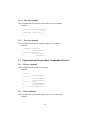
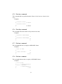
kalc User’s Manual
Eduardo M Kalinowski ([email protected])
Version 2.2.2
Contents
1
Introduction and Disclaimer
2
Using kalc – a brief tutorial
2.1 Reverse Polish Notation .
2.2 Other functions . . . . .
2.3 Complex numbers . . . .
2.3.1 Polar form . . .
2.4 Entering commands . . .
2.5 Getting help . . . . . . .
3
Running kalc
4
Using Readline
4.1 Readline essentials .
4.2 Killing text . . . . .
4.3 Numeric Arguments .
4.4 The history . . . . .
4.5 Other commands . .
7
.
.
.
.
.
.
.
.
.
.
.
.
.
.
.
.
.
.
.
.
.
.
.
.
.
.
.
.
.
.
.
.
.
.
.
.
.
.
.
.
.
.
.
.
.
.
.
.
.
.
.
.
.
.
.
.
.
.
.
.
.
.
.
.
.
.
.
.
.
.
.
.
.
.
.
.
.
.
.
.
.
.
.
.
.
.
.
.
.
.
.
.
.
.
.
.
.
.
.
.
.
.
.
.
.
.
.
.
.
.
.
.
.
.
.
.
.
.
.
.
.
.
.
.
.
.
.
.
.
.
.
.
7
8
8
8
9
9
9
9
.
.
.
.
.
10
10
11
11
11
12
5
Reusing the last arguments
5.1 Using lastarg for error recovery . . . . . . . . . . . . . . . . . . .
12
12
6
Working with other bases
6.1 Options relevant to hexadecimal strings . .
6.2 The current word size . . . . . . . . . . . .
6.3 Hexadecimal string operations . . . . . . .
6.3.1 Shifts and rotations . . . . . . . . .
6.4 Converting to and from hexadecimal strings
.
.
.
.
.
12
13
14
14
15
16
7
Using the memory
7.1 Listing and erasing the memory . . . . . . . . . . . . . . . . . .
7.2 Saving objects to disk . . . . . . . . . . . . . . . . . . . . . . . .
17
18
19
8
Other kinds of objects
8.1 Strings . . . . . . . . . . . . . . . . . . . . . . . . . . . . . . . .
8.2 Tagged objects . . . . . . . . . . . . . . . . . . . . . . . . . . .
8.3 Inf and NaN’s . . . . . . . . . . . . . . . . . . . . . . . . . . . .
19
19
19
20
9
The status file
20
.
.
.
.
.
.
.
.
.
.
.
.
.
.
.
.
.
.
.
.
.
.
.
.
.
1
.
.
.
.
.
.
.
.
.
.
.
.
.
.
.
.
.
.
.
.
.
.
.
.
.
.
.
.
.
.
.
.
.
.
.
.
.
.
.
.
.
.
.
.
.
.
.
.
.
.
.
.
.
.
.
.
.
.
.
.
.
.
.
.
.
.
.
.
.
.
.
.
.
.
.
.
.
.
.
.
.
.
.
.
.
.
.
.
.
.
.
.
.
.
.
.
.
.
.
.
.
.
.
.
.
.
.
.
.
.
.
.
.
.
.
.
.
.
.
.
.
.
.
.
.
.
.
.
.
.
.
.
.
.
.
.
.
.
.
.
.
.
.
.
.
10 Customization
10.1 Angle mode . . . . . . . . . . . . . .
10.2 Coordinate mode . . . . . . . . . . .
10.3 Number display format and precision .
10.4 Prompt . . . . . . . . . . . . . . . . .
10.5 Number of stack levels to display . . .
10.6 Screen width . . . . . . . . . . . . .
11 Arithmetic commands reference
11.1 The + command . . . . . . .
11.2 The - command . . . . . . .
11.3 The * command . . . . . . .
11.4 The / command . . . . . . .
11.5 The inv command . . . . . .
11.6 The mod command . . . . .
11.7 The chs and neg commands .
11.8 The abs command . . . . . .
11.9 The ceil command . . . . . .
11.10The floor command . . . . .
11.11The ip command . . . . . .
11.12The fp command . . . . . .
11.13The % command . . . . . .
11.14The %t command . . . . . .
11.15The %ch command . . . . .
11.16The gcd command . . . . . .
11.17The lcm command . . . . .
.
.
.
.
.
.
.
.
.
.
.
.
.
.
.
.
.
.
.
.
.
.
.
.
.
.
.
.
.
.
.
.
.
.
.
.
.
.
.
.
.
.
.
.
.
.
.
.
.
.
.
.
.
.
.
.
.
.
.
.
.
.
.
.
.
.
.
.
.
.
.
.
.
.
.
.
.
.
.
.
.
.
.
.
.
.
.
.
.
.
21
21
21
22
23
23
23
.
.
.
.
.
.
.
.
.
.
.
.
.
.
.
.
.
.
.
.
.
.
.
.
.
.
.
.
.
.
.
.
.
.
.
.
.
.
.
.
.
.
.
.
.
.
.
.
.
.
.
.
.
.
.
.
.
.
.
.
.
.
.
.
.
.
.
.
.
.
.
.
.
.
.
.
.
.
.
.
.
.
.
.
.
.
.
.
.
.
.
.
.
.
.
.
.
.
.
.
.
.
.
.
.
.
.
.
.
.
.
.
.
.
.
.
.
.
.
.
.
.
.
.
.
.
.
.
.
.
.
.
.
.
.
.
.
.
.
.
.
.
.
.
.
.
.
.
.
.
.
.
.
.
.
.
.
.
.
.
.
.
.
.
.
.
.
.
.
.
23
23
24
24
24
25
25
25
25
26
26
26
27
27
27
27
28
28
12 Exponential and Logarithmic Commands Reference
12.1 The exp command . . . . . . . . . . . . . . . . .
12.2 The ln command . . . . . . . . . . . . . . . . .
12.3 The ˆ command . . . . . . . . . . . . . . . . . .
12.4 The xroot command . . . . . . . . . . . . . . . .
12.5 The sq command . . . . . . . . . . . . . . . . .
12.6 The sqrt command . . . . . . . . . . . . . . . .
12.7 The expm1 command . . . . . . . . . . . . . . .
12.8 The lnp1 command . . . . . . . . . . . . . . . .
12.9 The log command . . . . . . . . . . . . . . . . .
12.10The alog command . . . . . . . . . . . . . . . .
12.11The cis command . . . . . . . . . . . . . . . . .
.
.
.
.
.
.
.
.
.
.
.
.
.
.
.
.
.
.
.
.
.
.
.
.
.
.
.
.
.
.
.
.
.
.
.
.
.
.
.
.
.
.
.
.
.
.
.
.
.
.
.
.
.
.
.
.
.
.
.
.
.
.
.
.
.
.
.
.
.
.
.
.
.
.
.
.
.
.
.
.
.
.
.
.
.
.
.
.
.
.
.
.
.
.
.
.
.
.
.
28
28
28
29
29
29
30
30
30
31
31
31
.
.
.
.
.
.
.
.
.
.
.
.
.
.
.
.
.
2
.
.
.
.
.
.
.
.
.
.
.
.
.
.
.
.
.
.
.
.
.
.
.
.
.
.
.
.
.
.
.
.
.
.
.
.
.
.
.
.
.
.
.
.
.
.
.
.
.
.
.
.
.
.
.
.
.
.
.
.
.
.
.
.
.
.
.
.
.
.
.
.
.
.
.
.
.
.
.
.
.
.
.
.
.
.
.
.
.
.
.
.
.
.
.
.
.
.
.
.
.
.
.
.
.
.
.
.
.
.
.
.
.
.
.
.
.
.
.
.
.
.
.
.
.
.
.
.
.
.
.
.
.
.
.
.
.
.
.
.
.
.
.
.
.
.
.
.
.
.
.
.
.
13 Trigonometric commands reference
13.1 The pi command . . . . . . . .
13.2 The sin command . . . . . . . .
13.3 The cos command . . . . . . . .
13.4 The tan command . . . . . . . .
13.5 The sec command . . . . . . . .
13.6 The csc command . . . . . . . .
13.7 The cot command . . . . . . . .
13.8 The asin command . . . . . . .
13.9 The acos command . . . . . . .
13.10The atan command . . . . . . .
13.11The atan2 command . . . . . . .
13.12The asec command . . . . . . .
13.13The acsc command . . . . . . .
13.14The acot command . . . . . . .
13.15The vers command . . . . . . .
13.16The hav command . . . . . . . .
13.17The d¿r command . . . . . . . .
13.18The r¿d command . . . . . . . .
.
.
.
.
.
.
.
.
.
.
.
.
.
.
.
.
.
.
.
.
.
.
.
.
.
.
.
.
.
.
.
.
.
.
.
.
.
.
.
.
.
.
.
.
.
.
.
.
.
.
.
.
.
.
.
.
.
.
.
.
.
.
.
.
.
.
.
.
.
.
.
.
.
.
.
.
.
.
.
.
.
.
.
.
.
.
.
.
.
.
.
.
.
.
.
.
.
.
.
.
.
.
.
.
.
.
.
.
.
.
.
.
.
.
.
.
.
.
.
.
.
.
.
.
.
.
.
.
.
.
.
.
.
.
.
.
.
.
.
.
.
.
.
.
.
.
.
.
.
.
.
.
.
.
.
.
.
.
.
.
.
.
.
.
.
.
.
.
.
.
.
.
.
.
.
.
.
.
.
.
.
.
.
.
.
.
.
.
.
.
.
.
.
.
.
.
.
.
.
.
.
.
.
.
.
.
.
.
.
.
.
.
.
.
.
.
.
.
.
.
.
.
.
.
.
.
.
.
.
.
.
.
.
.
.
.
.
.
.
.
.
.
.
.
.
.
.
.
.
.
.
.
.
.
.
.
.
.
.
.
.
.
.
.
.
.
.
.
.
.
.
.
.
.
.
.
.
.
.
.
.
.
.
.
.
.
.
.
.
.
.
.
.
.
.
.
.
.
.
.
.
.
.
.
.
.
.
.
.
.
.
.
.
.
.
.
.
.
.
.
.
.
.
.
31
31
32
32
32
32
33
33
33
34
34
34
35
35
35
36
36
36
36
14 Hyperbolic commands reference
14.1 The sinh command . . . . .
14.2 The cosh command . . . . .
14.3 The tanh command . . . . .
14.4 The sech command . . . . .
14.5 The csch command . . . . .
14.6 The coth command . . . . .
14.7 The asinh command . . . . .
14.8 The acosh command . . . .
14.9 The atanh command . . . . .
14.10The asech command . . . .
14.11The acsch command . . . .
14.12The acoth command . . . . .
14.13The gd command . . . . . .
14.14The invgd command . . . .
.
.
.
.
.
.
.
.
.
.
.
.
.
.
.
.
.
.
.
.
.
.
.
.
.
.
.
.
.
.
.
.
.
.
.
.
.
.
.
.
.
.
.
.
.
.
.
.
.
.
.
.
.
.
.
.
.
.
.
.
.
.
.
.
.
.
.
.
.
.
.
.
.
.
.
.
.
.
.
.
.
.
.
.
.
.
.
.
.
.
.
.
.
.
.
.
.
.
.
.
.
.
.
.
.
.
.
.
.
.
.
.
.
.
.
.
.
.
.
.
.
.
.
.
.
.
.
.
.
.
.
.
.
.
.
.
.
.
.
.
.
.
.
.
.
.
.
.
.
.
.
.
.
.
.
.
.
.
.
.
.
.
.
.
.
.
.
.
.
.
.
.
.
.
.
.
.
.
.
.
.
.
.
.
.
.
.
.
.
.
.
.
.
.
.
.
.
.
.
.
.
.
.
.
.
.
.
.
.
.
.
.
.
.
.
.
.
.
.
.
.
.
.
.
.
.
.
.
.
.
.
.
.
.
.
.
.
.
.
.
.
.
.
.
.
.
.
.
.
.
.
.
37
37
37
37
37
38
38
38
38
39
39
39
39
40
40
15 Stack manipulation commands reference
15.1 The dup command . . . . . . . . . . . . . . . . . . . . . . . . .
15.2 The dupdup command . . . . . . . . . . . . . . . . . . . . . . .
15.3 The ndupn command . . . . . . . . . . . . . . . . . . . . . . . .
40
40
40
41
.
.
.
.
.
.
.
.
.
.
.
.
.
.
3
.
.
.
.
.
.
.
.
.
.
.
.
.
.
15.4 The dup2 command .
15.5 The dupn command .
15.6 The drop command .
15.7 The nip command . .
15.8 The drop2 command
15.9 The dropn command
15.10The clear command .
15.11The swap command .
15.12The over command .
15.13The pick3 command
15.14The pick command .
15.15The unpick command
15.16The rot command . .
15.17The unrot command .
15.18The roll command . .
15.19The rolld command .
15.20The depth command
15.21The keep command .
.
.
.
.
.
.
.
.
.
.
.
.
.
.
.
.
.
.
.
.
.
.
.
.
.
.
.
.
.
.
.
.
.
.
.
.
.
.
.
.
.
.
.
.
.
.
.
.
.
.
.
.
.
.
.
.
.
.
.
.
.
.
.
.
.
.
.
.
.
.
.
.
.
.
.
.
.
.
.
.
.
.
.
.
.
.
.
.
.
.
.
.
.
.
.
.
.
.
.
.
.
.
.
.
.
.
.
.
16 Miscellaneous commands reference
16.1 The rand command . . . . . . .
16.2 The rdz command . . . . . . . .
16.3 The ! command . . . . . . . . .
16.4 The lgamma command . . . . .
16.5 The perm command . . . . . . .
16.6 The comb command . . . . . .
16.7 The min command . . . . . . .
16.8 The max command . . . . . . .
16.9 The sign command . . . . . . .
16.10The psign command . . . . . . .
16.11The mant command . . . . . . .
16.12The xpon command . . . . . . .
16.13The rnd command . . . . . . . .
16.14The type command . . . . . . .
16.15The vtype command . . . . . .
16.16The = command . . . . . . . . .
16.17The eval command . . . . . . .
16.18The shell command . . . . . . .
4
.
.
.
.
.
.
.
.
.
.
.
.
.
.
.
.
.
.
.
.
.
.
.
.
.
.
.
.
.
.
.
.
.
.
.
.
.
.
.
.
.
.
.
.
.
.
.
.
.
.
.
.
.
.
.
.
.
.
.
.
.
.
.
.
.
.
.
.
.
.
.
.
.
.
.
.
.
.
.
.
.
.
.
.
.
.
.
.
.
.
.
.
.
.
.
.
.
.
.
.
.
.
.
.
.
.
.
.
.
.
.
.
.
.
.
.
.
.
.
.
.
.
.
.
.
.
.
.
.
.
.
.
.
.
.
.
.
.
.
.
.
.
.
.
.
.
.
.
.
.
.
.
.
.
.
.
.
.
.
.
.
.
.
.
.
.
.
.
.
.
.
.
.
.
.
.
.
.
.
.
.
.
.
.
.
.
.
.
.
.
.
.
.
.
.
.
.
.
.
.
.
.
.
.
.
.
.
.
.
.
.
.
.
.
.
.
.
.
.
.
.
.
.
.
.
.
.
.
.
.
.
.
.
.
.
.
.
.
.
.
.
.
.
.
.
.
.
.
.
.
.
.
.
.
.
.
.
.
.
.
.
.
.
.
.
.
.
.
.
.
.
.
.
.
.
.
.
.
.
.
.
.
.
.
.
.
.
.
.
.
.
.
.
.
.
.
.
.
.
.
.
.
.
.
.
.
.
.
.
.
.
.
.
.
.
.
.
.
.
.
.
.
.
.
.
.
.
.
.
.
.
.
.
.
.
.
.
.
.
.
.
.
.
.
.
.
.
.
.
.
.
.
.
.
.
.
.
.
.
.
.
.
.
.
.
.
.
.
.
.
.
.
.
.
.
.
.
.
.
.
.
.
.
.
.
.
.
.
.
.
.
.
.
.
.
.
.
.
.
.
.
.
.
.
.
.
.
.
.
.
.
.
.
.
.
.
.
.
.
.
.
.
.
.
.
.
.
.
.
.
.
.
.
.
.
.
.
.
.
.
.
.
.
.
.
.
.
.
.
.
.
.
.
.
.
.
.
.
.
.
.
.
.
.
.
.
.
.
.
.
.
.
.
.
.
.
.
.
.
.
.
.
.
.
.
.
.
.
.
.
.
.
.
.
.
.
.
.
.
.
.
.
.
.
.
.
.
.
.
.
.
.
.
.
.
.
.
.
.
.
.
.
.
.
.
.
.
.
.
.
.
.
.
.
.
.
.
.
.
.
.
.
.
.
.
.
.
.
.
.
.
.
.
.
.
.
.
.
.
.
.
.
.
.
.
.
.
.
.
.
.
.
.
.
.
.
.
.
.
.
.
.
.
.
.
.
.
.
.
.
.
.
.
.
.
.
.
.
.
.
.
.
.
.
.
.
.
.
.
.
.
.
.
.
.
.
.
.
.
.
.
.
.
.
.
.
.
.
.
.
41
41
42
42
42
43
43
43
43
44
44
44
45
45
46
46
46
47
.
.
.
.
.
.
.
.
.
.
.
.
.
.
.
.
.
.
47
47
47
47
47
48
48
48
48
48
49
49
49
50
50
51
51
51
51
17 Time and date commands reference
17.1 The date command . . . . . . .
17.2 The time command . . . . . . .
17.3 The ¿hms command . . . . . . .
17.4 The hms¿ command . . . . . . .
17.5 The date+ command . . . . . .
17.6 The ddays command . . . . . .
17.7 The hms+ command . . . . . .
17.8 The hms- command . . . . . . .
17.9 The dow command . . . . . . .
17.10The dowstr command . . . . . .
17.11The tstr command . . . . . . . .
.
.
.
.
.
.
.
.
.
.
.
.
.
.
.
.
.
.
.
.
.
.
.
.
.
.
.
.
.
.
.
.
.
.
.
.
.
.
.
.
.
.
.
.
.
.
.
.
.
.
.
.
.
.
.
.
.
.
.
.
.
.
.
.
.
.
.
.
.
.
.
.
.
.
.
.
.
.
.
.
.
.
.
.
.
.
.
.
.
.
.
.
.
.
.
.
.
.
.
.
.
.
.
.
.
.
.
.
.
.
.
.
.
.
.
.
.
.
.
.
.
.
.
.
.
.
.
.
.
.
.
.
.
.
.
.
.
.
.
.
.
.
.
.
.
.
.
.
.
.
.
.
.
.
.
.
.
.
.
.
.
.
.
.
.
.
.
.
.
.
.
.
.
.
.
.
.
.
.
.
.
.
.
.
.
.
.
51
52
52
52
52
53
53
53
53
54
54
54
18 Complex number commands reference
18.1 The r¿c command . . . . . . . . . .
18.2 The re¿c command . . . . . . . . .
18.3 The im¿c command . . . . . . . . .
18.4 The c¿r command . . . . . . . . . .
18.5 The re command . . . . . . . . . .
18.6 The im command . . . . . . . . . .
18.7 The conj command . . . . . . . . .
18.8 The arg command . . . . . . . . . .
.
.
.
.
.
.
.
.
.
.
.
.
.
.
.
.
.
.
.
.
.
.
.
.
.
.
.
.
.
.
.
.
.
.
.
.
.
.
.
.
.
.
.
.
.
.
.
.
.
.
.
.
.
.
.
.
.
.
.
.
.
.
.
.
.
.
.
.
.
.
.
.
.
.
.
.
.
.
.
.
.
.
.
.
.
.
.
.
.
.
.
.
.
.
.
.
.
.
.
.
.
.
.
.
.
.
.
.
.
.
.
.
.
.
.
.
.
.
.
.
.
.
.
.
.
.
.
.
55
55
55
55
55
56
56
56
56
.
.
.
.
.
.
.
.
.
.
57
57
57
57
58
58
58
59
59
59
59
.
.
.
.
60
60
60
60
61
19 Relational commands reference
19.1 The == command . . . . . .
19.2 The != and # commands . .
19.3 The ¡ command . . . . . . .
19.4 The ¿ command . . . . . . .
19.5 The ¡= command . . . . . .
19.6 The ¿= command . . . . . .
19.7 The and command . . . . . .
19.8 The or command . . . . . .
19.9 The xor command . . . . . .
19.10The not command . . . . . .
20 String commands reference
20.1 The + command (for strings)
20.2 The size command . . . . .
20.3 The ¿str command . . . . . .
20.4 The str¿ command . . . . . .
.
.
.
.
.
.
.
.
.
.
.
.
.
.
5
.
.
.
.
.
.
.
.
.
.
.
.
.
.
.
.
.
.
.
.
.
.
.
.
.
.
.
.
.
.
.
.
.
.
.
.
.
.
.
.
.
.
.
.
.
.
.
.
.
.
.
.
.
.
.
.
.
.
.
.
.
.
.
.
.
.
.
.
.
.
.
.
.
.
.
.
.
.
.
.
.
.
.
.
.
.
.
.
.
.
.
.
.
.
.
.
.
.
.
.
.
.
.
.
.
.
.
.
.
.
.
.
.
.
.
.
.
.
.
.
.
.
.
.
.
.
.
.
.
.
.
.
.
.
.
.
.
.
.
.
.
.
.
.
.
.
.
.
.
.
.
.
.
.
.
.
.
.
.
.
.
.
.
.
.
.
.
.
.
.
.
.
.
.
.
.
.
.
.
.
.
.
.
.
.
.
.
.
.
.
.
.
.
.
.
.
.
.
.
.
.
.
.
.
.
.
.
.
.
.
.
.
.
.
.
.
.
.
.
.
.
.
.
.
.
.
.
.
.
.
.
.
.
.
.
.
.
.
.
.
.
.
.
.
.
.
.
.
.
.
.
.
.
.
.
.
.
.
.
.
.
.
.
20.5 The num command . . . . . .
20.6 The chr command . . . . . . .
20.7 The head command . . . . . .
20.8 The tail command . . . . . . .
20.9 The pos command . . . . . . .
20.10The sub command . . . . . . .
20.11The repl command . . . . . .
20.12The str¿id and $¿id commands
20.13The id¿str and id¿$ commands
.
.
.
.
.
.
.
.
.
.
.
.
.
.
.
.
.
.
.
.
.
.
.
.
.
.
.
.
.
.
.
.
.
.
.
.
.
.
.
.
.
.
.
.
.
.
.
.
.
.
.
.
.
.
.
.
.
.
.
.
.
.
.
.
.
.
.
.
.
.
.
.
.
.
.
.
.
.
.
.
.
.
.
.
.
.
.
.
.
.
.
.
.
.
.
.
.
.
.
.
.
.
.
.
.
.
.
.
.
.
.
.
.
.
.
.
.
.
.
.
.
.
.
.
.
.
.
.
.
.
.
.
.
.
.
.
.
.
.
.
.
.
.
.
.
.
.
.
.
.
.
.
.
.
.
.
.
.
.
.
.
.
.
.
.
.
.
.
.
.
.
61
61
61
62
62
62
63
63
63
21 Memory commands reference
21.1 The sto command . . . . . . .
21.2 The rcl command . . . . . . .
21.3 The purge command . . . . .
21.4 The clvar and clusr commands
21.5 The clvar command . . . . .
21.6 The coldstart command . . . .
21.7 The vars command . . . . . .
21.8 The disksto command . . . . .
21.9 The diskrcl command . . . . .
21.10The pwd command . . . . . .
21.11The cd command . . . . . . .
.
.
.
.
.
.
.
.
.
.
.
.
.
.
.
.
.
.
.
.
.
.
.
.
.
.
.
.
.
.
.
.
.
.
.
.
.
.
.
.
.
.
.
.
.
.
.
.
.
.
.
.
.
.
.
.
.
.
.
.
.
.
.
.
.
.
.
.
.
.
.
.
.
.
.
.
.
.
.
.
.
.
.
.
.
.
.
.
.
.
.
.
.
.
.
.
.
.
.
.
.
.
.
.
.
.
.
.
.
.
.
.
.
.
.
.
.
.
.
.
.
.
.
.
.
.
.
.
.
.
.
.
.
.
.
.
.
.
.
.
.
.
.
.
.
.
.
.
.
.
.
.
.
.
.
.
.
.
.
.
.
.
.
.
.
.
.
.
.
.
.
.
.
.
.
.
.
.
.
.
.
.
.
.
.
.
.
.
.
.
.
.
.
.
.
.
.
.
.
.
.
.
.
.
.
.
.
.
.
64
64
64
64
64
64
64
65
65
65
65
65
6
1
Introduction and Disclaimer
This document describes kalc version 2.2.2, a full-featured scientific calculator
using Reverse Polish Notation (see section 2.1). It includes many functions, and a
built-in help system (see section 2.5).
kalc can work with real and complex numbers, and also with strings. It includes “unlimited” memory to store any object that can be put in the stack. (“Unlimited” here means that there is no arbitrary limit on the size of the memory.
Obviously, you cannot store, for example, a 2Gb string in memory if you don’t
have that amount of RAM (or disk space, if your system supports virtual memory
and swapping.)
The behaviour of kalc is very similar to the one of a HP48 or HP49 calculator.
It is not, however, a HP48 emulator nor it uses any code from its ROM.
The source code of kalc distributed. For instructions on how to compile and
install it, see the file INSTALL. There is also a package with a pre-compiled MSDOS executable.
You may distribute kalc freely, but only in its whole, unmodified form. You
are allowed to make modifications to this program, but if you do so, you must not
redistributed your modificated version. For details, see the file COPYING.
The above conditions do not necessarily apply to the GNU Readline Library,
used by this program. See the file COPYING.lib for details on the conditions of
use and redistribution of that library.
This program is distributed in the hope it will be useful, but it comes without
any kind of warranty. Use it at your onw risk.
2
Using kalc – a brief tutorial
To run kalc, just enter kalc at your shell prompt. If this is the first time you run the
program, you’ll see a message saying “Status file invalid/inexistent – using default
settings”. Ignore that message for now. You’ll then see a > prompt. Whenever you
see this prompt you can enter commands. For example, enter 2 3 +. You’ll see
the result (5), and another prompt.
The entire section up to the above should look like this:
$ kalc
Status file invalid/inexistent -- using default settings
kalc v2.2.2, Copyright (C) 1999-2000 Eduardo M Kalinowski ([email protected])
> 2 3 +
1:
5
7
>
The fact that there is prompt showing means that you can enter more commands. For example, let’s divide the above result by 3. Just enter 3 / and press
ENTER. The result is shown.
2.1
Reverse Polish Notation
As you may have noted from the above two calculations, the operator (the + or the
/) has come after the operands (the numbers.) This curious thing is called Reverse
Polish Notation.
In RPN, the operators always come after the operands. For example, the expression (5 + 2)/3 would be written as “5 2 + 3 /”. The order of evaluation is from
left to right always; parenthesis are never necessary.
kalc uses a stack to do its calculations. kalc’s stack is just like a pile of plates:
the first plate put on the pile is the last one to be used. The difference is that kalc’s
stack is upside down, ie, the “plates” are put (and thus removed) from the bottom.
When you enter a number, it is put in the bottom of the stack, and any numbers
previously there are shifted up. The operations you do remove numbers from the
bottom of the stack, and them put their result(s) again in the bottom of the stack.
The bottommost stack level is numbered “1”. The above levels get increasing
numbers. Most calculations will take their arguments from level one (and sometimes level two also), and return their result to level one.
The stack in kalc doesn’t have a fixed size, it is only limited by the amount of
available memory. But only the four bottommost are displayed by default. (This
can be changed, see sections 3 and 10.5.) If you want to see more, use the =
command (see section 16.16.)
2.2
Other functions
Besides the basic arithmetic operators, kalc has a lot of built-in scientific functions.
Try, for example, sin, exp, cosh. Remember that first you put the argument in
the stack, then you run the function.
All mathematical functions are called in kalc by their symbols. So, even if I
haven’t told you how to do it, you can probably guess how to calculate the hyperbolic arc tangent of a number.
2.3
Complex numbers
kalc can work with complex numbers, too. To put a complex number in the stack,
use the following syntax: (x, y), where x is the real part and y is the imaginary
8
part. You can omit the space or comma delimiting the two parts, but not both.
Almost all operations that can be applied to real numbers can also be used
with complex numbers. This included not only the basic functions like + but also
functions like cosh or ln.
2.3.1
Polar form
Complex numbers can be entered and/or displayed in their polar forms. The format
is (r, <theta), where r is the magnitude and theta is the angle. You may
omit the space and/or the comma if you wish.
To configure kalc to display complex numbers in polar form, see section 10.2.
The current angle mode (degrees or radians) is used to display the angle of
complex numbers. Refer to section 10.1 to learn how to change the angle mode.
2.4
Entering commands
The most basic way to enter a command (and seldom used) is to enter that command and press ENTER. However, you can enter more than one command at a
time, just separate them with spaces. Numbers should also be separated from commands and other numbers with a space.
If you just press ENTER without entering any command, the stack will be
shown.
The case is not important when entering commands. dup is the same as DUP
or dUp.
This program uses the GNU Readline Library. This allows you to edit the line
with the commands using many powerful features. The most basic ones are moving
the cursor and inserting text in arbitrary locations. But there is much more. See
section 4 or the GNU Readline Manual for more information on what you can do.
2.5
Getting help
At any time, you can use the help command to get help. If you just type “help”,
you’ll get a list of commands. To get help on a particular command, use help
followed by that command’s name, for example help sin.
3
Running kalc
kalc supports a few command line options that control its behaviour. The syntax
is:
kalc [options] [--] [commands]
9
The options are -d, -s, -m, -b, --help and --version. Any unprocessed
options will be taken as commands, and these will be executed as if they had been
entered on the prompt. If you use -- anywhere on the command line, everything
that follows will be considered a command, even if it starts with a -.
The -d option must be followed by a numeric argument. It specifies how
many levels of the stack will be shown by default. If you want the whole stack to
be shown always, specify -1 as the argument. Note that if the argument is 0, the
stack will not be displayed.
If this option is present, it overrides the number saved in the status file (see
section 9.)
The -s and -m options tell kalc not to load the stack and memory, respectively,
from the status file (see section 9.)
The -b options specifies that kalc should be run in batch mode. After processing all the commands in the command line and printing the stack, it exits.
The --help option prints a help message describing the command line options and exits successfully. The --version option prints kalc’s version and
exits successfully.
4
Using Readline
kalc uses the GNU Readline Library. This allows you to edit the commands you’ve
entered as if you were using a text editor. You can move the cursor, insert or delete
text, and much more. If you are familiar with Readline, you probably want to
skip this section. This is because the Readline library provides a consistent user
interface between all programs that use it.
4.1
Readline essentials
You can enter characters as usual. Just type them, and they’ll appear on the
screen. Use the Backspace key (or the Delete key, if your keyboard doesn’t have
a Backspace key) to delete the last character. To move the cursor, use the left and
right arrow keys. If your keyboard doesn’t have arrow keys, the keys Control-b and
Control-f will move the cursor to the left and right, respectively. To move forward
or backward a word, use the Alt-b and Alt-f keys. The “Alt” key may be labelled
“Edit” on some keyboards. If you don’t have an Alt or Edit key, press ESC, release
it and then press b (or f). This combination works for all commands that use the
Alt key.
To move to the beginning of the line, use Control-a. To move to the end of the
line, use Control-e.
10
Another useful command is Control- (underscore). It undoes the last action.
So, if you make a mistake, just press Control- to undo it.
4.2
Killing text
Killing means deleting text from a line, but saving it somewhere it can be later
brought again. The operation of bringing back killed text is called “yanking”.
Whenever you use one of the kill commands, the text is saved in the “kill ring”.
Any number of consecutive kills saves the text together, so when you yank it you’ll
get it all back. The kill-ring is not line-specific, you may yank text from a previous
line.
The most frequently used kill and yank commands are:
Control-k Kill text from the cursor position to the end of the line.
Alt-d Kill from the cursor postion to the end of the current word, or, if between
words, to the end of the next word.
Alt-Backspace (or Alt-Del in some computers) Kill from the cursor postion to
the start of the current word, or, if between words, to the start of the previous
word.
Control-y Yank the most recently killed text back at the cursor position.
Alt-y Rotate the kill-ring. This command can only be used if the previous command was Control-y or Alt-y. This replaces the last yanked text with the text
that was killed before it.
4.3
Numeric Arguments
Most Readline commands support numeric arguments. For example, if you give
the argument 5 to the command Control-f (go forward a character) it goes five
characters forward.
To enter an argument to a command, press Alt and the argument digit simultaneously. For example, to give the Control-f command an argument of 10, press
Alt-1 0 Control-f. Arguments can also be negative, if you press Alt– (hyphen) as
the first argument digit. If you just specify “-” as argument, it is equivalent to -1.
4.4
The history
All commands you type are saved in the history. To cycle through the commands in
the history in order, use the up and down arrow keys or the Control-p and Control-n
keys.
11
To search the history for a specific entry, press Control-r then enter part of the
command. As your entry matches the history lines, they are shown. When you’ve
found what you wanted, press Enter to execute the command or any other key to
execute the action bound to that key. To finish a search, use Control-g.
4.5
Other commands
In kalc, use the Tab key to insert the element in level one at the command line.
With an argument, inserts the number at the given level.
There are also many other commands for Readline, and it can also be customized for your personal taste. For more information, see the Readline manual.
5
Reusing the last arguments
Everytime you run a command, its arguments are stored in a special area called the
“last arguments list”, or “lastarg” for short. You can bring the commands from that
list with the lastarg command. Here is an example of its use:
> 6 9 *
1:
> lastarg
3:
2:
1:
> +
2:
1:
5.1
54
54
6
9
54
15
Using lastarg for error recovery
The memory commands purge and sto (see 7) have a slightly different behavior
regarding the last arguments.
When you run the purge command, the former contents of that variable are
stored (and also the name), so that you can restore the variable with lastarg
sto.
The sto command stores the name and the former contents of that variable, so
that you can recover from an accidental sto with lastarg sto lastarg.
6
Working with other bases
kalc can work with integers (but not real numbers) in bases other than 10. You can
convert numbers to and from any base between 2 and 10, and do several kinds of
12
manipulation to them.
To work with numbers in other bases, a new kind of object is used: the hexadecimal string (or hxs for short.) The name “string” comes from the HP48, and
is kept for consistency, however, in kalc these objects are more closely related to
integers. Despite the name, all bases from 2 to 10 can be used.
The syntax of that object is:
# <number><base specifier>
After the # sign, you may put spaces. However, the base specifier must not be
separated from the number.
The number is simply the representation of the number. The valid characters
depend on the base used (see below.) For bases greater than 10, the letter “a”
represents 11, “b” represents 12, and so on. You can enter the letters in upper or
lower case (but there is a catch — read on.)
The base specifier is an at sign (@) followed by the base (which is always
written in decimal.) So, base 2 is represented as @2 and base 27 is @27.
For the most commonly used bases 2, 8, 10, and 16 there are some shortcuts:
appending a “b” after the number makes it binary (the same as “@2”,) an “o” represents octal, a “d” decimal and “h”. When the hexadecimal strings are displayed,
that notation is also used.
If you do not specify a base, then the current base (see section 6.1) will be
used to parse the number. You must be careful, however, because if the number
ends with a lowercase “b”, “o”, “d” or “h”, that will be taken as a base specifier. To
avoid that happening, you can end the number with an uppercase letter or explicitly
specify the base.
Here are some examples, all of them represent the number 123:
#
#
#
#
#
#
#
#
6.1
1111011b
443@5
173o
123d
A3@12
7Bh
4N@25
3F@36
Options relevant to hexadecimal strings
There are two options that are relevant to hexadecimal strings: the current base and
word size.
The current base is the base that the numbers will be displayed in the stack, and
the numbers entered without a explicit base will be parsed in that base.
13
To set the base, use the set command:
> set base x
where x is the desired base, between 2 and 36. For the bases 2, 8, 10 and
16, you can use set base bin, set base oct, set base dec and set
base hex, respectively. You can also simply type bin, oct, dec or hex.
6.2
The current word size
The current word size affects the way that numbers are displayed and used in calculations.
The word size can be this way:
> set wordsize x
where x is the desired word size. The minimum value is 1, the maximum
depends on your system. When kalc was built, it checked wheter 64-bit numbers
were available. If possible, they were used. If not, then 32-bit numbers were used.
If you don’t know the maximum word size, then just enter a big number such as
99, and kalc will use the greates word size possible. You can see the base with the
show wordsize command.
Another way to set the current word size is by putting a real number or an
hex string in the stack representing the desired word size and then run the stws
command. The rcws command puts in the stack a real number representing the
current word size.
Whenever an hexadecimal number is displayed, it is truncated to the n least
significant bits, where n is the current word size setting. Whenever you do some
operation on an hexadecimal number (see section 6.3, the result is also truncated to
the current word size. Shifts and rotations (see section 6.3.1) only change the least
significant bits, and the result is then truncated.
6.3
Hexadecimal string operations
All arithmetic commands also work for hexadecimal strings. You can add, subtract, divide and multiply hexadecimal strings normally. You can even mix real
numbers in the calculation: they will be automatically be converted to hexadecimal strings (but the fractional part will be lost.) The neg command produces the
two’s complement of the number.
14
6.3.1
Shifts and rotations
kalc includes a wide variety of commands for shifting and rotating the hexadecimal
string bits. They all take into consideration the current word size (see section 6.2.)
The available commands are:
sl This command shifts the hxs one bit to the left. The most significant bit is lost.
Here is an example, assuming the current word size is 4:
1:
> sl
1:
> sl
1:
# 1011b
# 110b
# 1100b
slb This command shifts the hxs one byte to the left. The most significant byte is
lost. Here is an example, assuming the current word size is 32:
1:
> slb
1:
> slb
1:
# CAFEBABEh
# FEBABE00h
# BABE0000h
sr This command shifts the hxs one bit to the right. The least significant bit is lost.
Here is an example, assuming the current wordsize is 4:
1:
> sr
1:
> sr
1:
# 1101b
# 110b
# 11b
asr This command does an arithmetic shift one bit to the right. The most significant bit is preserved in the operation. The least significant bit is lost. Here is
an example, assuming the current word size is 4:
1:
> asr
1:
> asr
1:
# 1010b
# 1101b
# 1110b
srb This command shifts the hxs one byte to the right. The least significant byte
is lost. Here is an example, assuming the current word size is 32:
15
1:
> srb
1:
> srb
1:
# DEADBEEFh
# DEADBEh
# DEADh
rl This command rotates the hxs one bit to the left. Here is an example, assuming
the current word size is 4:
1:
> rl
1:
> rl
1:
# 1101b
# 1011b
# 111b
rlb This command rotates the hxs one byte to the left. Here is an example, assuming the current word size is 32:
1:
> rlb
1:
> rlb
1:
# CAFEBABEh
# FEBABECAh
# BABECAFEh
rr This command rotates the hxs one bit to the right. Here is an example, assuming
the current word size is 4:
1:
> rr
1:
> rr
1:
# 1001b
# 1100b
# 110b
rrb This command rotates the hxs one byte to the right. Here is an example,
assuming the current word size is 32:
1:
> rrb
1:
> rrb
1:
6.4
# DEADBEEFh
# EFDEADBEh
# BEEFDEADh
Converting to and from hexadecimal strings
There are two commands for converting to and from hexadecimal strings. Here
they are:
16
r>b This command converts the real number in level one to an hexadecimal string.
The fractional part is discarded. Example:
1:
> r>b
1:
> 413442.4321
2:
1:
> r>b
2:
1:
12345
# 12345d
# 12345d
413442.4321
# 12345d
# 413442d
b>r This command converts an hexadecimal string to a real number. Example:
1:
> b>r
1:
7
# 134214d
134214
Using the memory
Besides the stack, you can store all objects that can be present in kalc’s stack in
the memory, a permanent place of storage. The memory has no fixed size, you can
store as many objects as your computer’s memory and disk can hold.
To store an object in memory, you must give it a name, which will be later used
to bring it back when you want. Such names in kalc are called identifiers. It is a
piece of text delimited by single quotes. Unlike in the HP48, identifiers in kalc can
have any characters, even those not allowed on the HP48 such as +, *, space, etc.
The identifier may even be a null identifier: ’’. When entering the identifier, you
may include a single quote in it using the \’ escape sequence.
To store an object, put that object in level two of the stack and an identifier in
level one. Then, just run the command sto and the object is stored.
To recall an object from the stack, put in level one the identifier, and run the
rcl command. A copy of the object is put in level one. The original object is not
affected: you may recall it again if you want.
There is an easier way to recall objects: instead of putting the identifier on the
stack (delimited by single quotes), just enter the identifier as if it were a command,
without the quotes. You’ll get the object in the stack. If there is no object with that
name, you’ll end up with the identifier in the stack. However, this shortcut will not
work if the identifier has spaces in it. In this case, you’ll need to use the standard
approach.
17
The memory is stored in the status file (see section 9). When starting kalc, you
can use the -m option to prevent the memory from being loaded. For more details
on this, see section 3.
Here are some examples of the usage of the memory:
> pi
1:
3.14159265358979
> ’AConstant’
2:
3.14159265358979
1:
’AConstant’
> sto
> ’AConstant’
1:
’AConstant’
> rcl
1:
3.14159265358979
> AConstant
2:
3.14159265358979
1:
3.14159265358979
7.1
Listing and erasing the memory
When you want to see all the objects stored in memory, you can use the vars
command. It will output a list of all objects in memory. Here is an example (continuation of the previous):
> 1 exp ’Another Constant’
2:
2.71828182845905
1:
’Another Constant’
> sto
> "Hello World"
1:
"Hello World"
> ’String’
2:
"Hello World"
1:
’String’
> sto
> (3, -2) ’cmp’ sto
> vars
’AConstant’ ’cmp’ ’String’
’Another Constant’
To erase one object from the memory, put that object’s identifier in the stack
and run the purge command.
If you want to erase the whole memory, use the clvar command. This command will erase all your memory and there is no way of bringing it back. Because of this, the command asks your for confirmation before doing the operation.
18
7.2
Saving objects to disk
In addition to saving objects in kalc’s memory, objects can also be saved to the
disk. To do this, put the object in level two, and the path of the file you want to
save in level one (this is an identifier). Then run the disksto command. The
object will be saved to the named file.
To recall an object from a file, put the file’s path (an identifier) in the stack, and
run the diskrcl command. If the file contains a valid object, it will be loaded in
level one.
If you give a relative path as the name of the file, it is considered as relative
to the current working directory. To discover which directory is this, run the pwd
command. It will output the directory. To change the current directory, put the
directory you want to go to in level one (an identifier) and run the cd command.
8
8.1
Other kinds of objects
Strings
In addition to being able of manipulating numbers, kalc can also work with strings.
To include a string in the stack, surround it with double quotes, for example:
> "This is a string"
1:
"This is a string"
>
When entering a string, you may include a new-line character with the escape
sequence \n or a double-quote with \".
8.2
Tagged objects
Any object in kalc can have a tag, a short (or long, if you wish) string that identifies
it. To create a tagged object, prefix it with :tag:, where tag is the name you
want to give to the object.
To give an existing object a tag, put that object in level two and the tag (a string,
or any other object, which will be converted to a string) in level one, and run the
>tag command. Here are some examples:
> :Tag: 12345
1:
> (12 -5)
2:
1:
> Result
Tag: 12345
Tag: 12345
(12,-5)
19
3:
2:
1:
> >tag
2:
1:
Tag: 12345
(12,-5)
’Result’
Tag: 12345
Result: (12,-5)
You can work with tagged objects as if they were normal objects. The tags will
be removed, however, if you do any operation on them.
To strip all tags from an object, use the dtag command.
8.3
Inf and NaN’s
Provided your system supports it, kalc has support for non-stop calculations. This
means you’ll never get an error while you’re doing your calculations, except if you
do not enter enough arguments or if you mistake the argument type. But you’ll not
get an error for dividing 1 by 0, or even 0 by 0.
To achieve this, two concepts are important: Inf and NaN. You’ll get Inf as
a result whenever you run a function which an argument that would result in a
very large result, such as 1e300 * 1e300, or 2 divided by 0. You can read ”Inf” as
infinity, and that’s what it means. Its complement is -Inf, which is negative infinity.
The other concept is NaN (short for not-a-number). You get this result when
the result of a function you called is undefined, such as 0/0, Inf-Inf, and so on.
If you want to get one of this values in the stack, you can just use the commands
inf, -inf and nan.
9
The status file
You do not have to worry about losing your work when you exit kalc. You can
save the state of the calculator and load it again whenever necessary. You can even
keep several saved states. This is achieved with the status files.
When kalc is started, it reads the last file that was used. If you haven’t told
kalc to use a different file, it will be a file called .kalc on your home directory (if
you are using a UNIX system) or kalc.ini in the current directory (if you are
using a MS-DOS system). In this file, all your preferences are saved (see section
10), the last arguments (see section 5), the stack (see section 2.1 and the memory
(see section 7).
When you exit kalc, the status file is saved automatically. If for some reason
you do not want this to happen, exit kalc with the abort command. This will not
save the status file. At any moment, you can use the save command to save the
status.
20
If you want to open another status file, put its name in the stack (a identifier),
and run the open command. If it is necessary, you’ll be asked to save the current
if. Then, the new file will be opened.
To save the current status under a different name, use the saveAs command.
Just put the file name (as an identifier) in level one, and run the command.
If for some reason you want to reset kalc to its default state, run the coldstart command. Note that this will erase the memory, the stack, the last arguments and return all the preferences to their default values without asking for
confirmation.
10
Customization
Several aspects of kalc can be customized. These include, for example, the way to
display numbers and the angle mode. The commands that allow this are set and
show.
The set command, as you might have guessed, sets a specific option in kalc.
A few of these options can also be set in a different way, more RPN-like. Details
will be given in the appropriate sections. The show command displays the current
value for a specific option.
Both commands, if given no option after it, display a list of options (equivalent
to typing help show).
10.1
Angle mode
The angle mode can be set to either radians (the default) or degrees. To set it, use
the set command this way:
> set anglemode {deg|rad}
Choosing the one you want. Or you can use the commands deg and rad to
select degress and radians, respectively.
Note: when dealing with complex numbers, the angle mode is ignored, and is
assumed to be always radians.
10.2
Coordinate mode
The coordinate used to represent complex numbers system can be set to rectangular
(the default) or polar. It is set this way:
> set coordinate {rect|cylin}
21
Specifying rect selects rectangular coordinates, and cylin specifies cylindrical (polar) coordinates. You can also select rectangular mode with the rect
command, and polar mode with the commands polar and cylin (both are equivalent.)
10.3
Number display format and precision
These options are closely related. The number display format specifies how the
numbers will be shown (the four available formats are described below), and the
precision the number of decimal places to show in each mode. Note that precision
does not really alter the precision of the calculator; all calculations are done using
all possible precision numbers, but not all must be shown should you want it this
way.
To set the number format, use the command
> set number-format &lcub;std|fix|sci|eng&rcub;
The available number formats are:
std The “standard” mode is the common mode for displaying numbers: if possible,
the number is not displayed in scientific notation, and decimal places are only
shown if they are present. Up to 15 decimal places may be shown, but no
trailing zeros are added.
fix The “fixed precision” mode always display the number of decimal places specified by the precision option. Trailing zeros are added if necessary.
sci The “scientific notation” mode always displays numbers using scientific notation, with the number of decimal places specified by the precision option.
eng The “engineering notation” mode displays precision + 1 significant digits using engineering notation. Engineering notation is like scientific notation, but
the exponent is always a multiple of three.
To set the precision, use the set command as follows:
> set precision <n>
Where <n> is the number of decimal places you want. It must be between zero
and fifteen, inclusive. Numbers less than zero are treated as zero, and numbers
greater than fifteen are treated as fifteen. Only the integer part of the argument is
considered.
Note that the precision is ignored for the std mode.
You can also set the precision with the commands std, fix, sci and eng.
All but std take an argument in level one: the precision.
22
10.4
Prompt
You can change the prompt for commands kalc uses. You can set it to anything
you want, up to 20 characters. Use the set command to change it:
> set prompt <text>
If you want to include spaces in the prompt, surround the entire prompt with
double quotes.
10.5
Number of stack levels to display
By default, kalc displays only the bottommost four stack levels. You can change
this number with the set lines command.
This option can be temporarily overriden with the = command (see section
16.16).
10.6
Screen width
The width of the screen can be set this way:
> set width <n>
Where <n> is the number of columns. The default is 78. The minimum is 25,
values less than that will be rejected.
11
11.1
Arithmetic commands reference
The + command
This command adds two numbers.
Examples:
> 12.5
1:
> 3.7
2:
1:
> +
1:
> (1, 3) (-2 4)
3:
2:
1:
12.5
12.5
3.7
16.2
16.2
(1,3)
(-2,4)
23
> +
2:
1:
11.2
16.2
(-1,7)
The - command
This command subtracts two numbers.
Examples:
> 15.7 3.2
2:
1:
> 1:
> (4 -3) (1 -1)
3:
2:
1:
> 2:
1:
11.3
15.7
3.2
12.5
12.5
(4,-3)
(1,-1)
12.5
(3,-2)
The * command
This command multiplies two numbers.
Examples:
> 3.4 -5.2 *
1:
> (4, 2) (3 -1) *
2:
1:
11.4
-17.68
-17.68
(14,2)
The / command
This command divides two numbers.
Examples:
> 10 3 /
1:
3.33333333333333
> (4 8) (2 2)
3:
3.33333333333333
2:
(4,8)
1:
(2,2)
> /
2:
3.33333333333333
1:
(3,1)
24
11.5
The inv command
This command returns one divided by a number.
Examples:
> 5 inv
1:
> (4 2)
2:
1:
> inv
2:
1:
11.6
0.2
0.2
(4,2)
0.2
(0.2,-0.1)
The mod command
This command returns the remainder of the division of y (level two) and x (level
one).
Example:
> 10 3 mod
1:
11.7
1
The chs and neg commands
Thesse commands change the sign of a number.
Examples:
> 4
1:
> chs
1:
> neg
1:
11.8
4
-4
4
The abs command
This command returns the absolute value of a number. For real numbers, this is
equal to the number without its sign. For complex number, it is the square root of
the sum of the squares of the real and imaginary parts.
Examples:
> 4 abs
1:
> -5 abs
4
25
2:
1:
> (3 4)
3:
2:
1:
> abs
3:
2:
1:
11.9
4
5
4
5
(3,4)
4
5
5
The ceil command
This command returns the smallest integer greater than or equal to its input.
Examples:
> 3.9 ceil
1:
> -3.9 ceil
2:
1:
11.10
4
4
-3
The floor command
This command returns the greatest integer less than or equal to its input.
Examples:
> 3.9 floor
1:
> -3.9 floor
2:
1:
11.11
3
3
-4
The ip command
This command returns the integer part of its input.
Examples:
> pi
1:
> ip
1:
3.14159265358979
3
26
11.12
The fp command
This command returns the fractional part of its input.
Examples:
> pi
1:
> fp
1:
11.13
3.14159265358979
0.141592653589793
The % command
This command returns y (level two) percent of x (level one).
Examples:
> 200 25 %
1:
> 314 13.9 %
2:
1:
11.14
50
50
43.646
The %t command
This command returns the percent of the level two argument that is represented by
the level one argument.
Examples:
> 200 25 %t
1:
> 520 52 %t
2:
1:
11.15
12.5
12.5
10
The %ch command
This command returns the percentage change from y (level two) to x (level 1) as a
percentage of y.
Examples:
> 150 175 %ch
1:
16.6666666666667
> 215 190 %ch
2:
16.6666666666667
1:
-11.6279069767442
27
11.16
The gcd command
This command returns the greatest common divisor of two numbers.
Examples:
> 411056775237 61754894058 gcd
1:
1257
> 895324789 3745907 gcd
2:
1257
1:
1
11.17
The lcm command
This command returns the least common multiple of two numbers.
Examples:
> 799984123 239874 lcm
1:
191895391520502
> 104890 2349002 lcm
2:
191895391520502
1:
123193409890
12
12.1
Exponential and Logarithmic Commands Reference
The exp command
This command returns e raised to its argument.
Examples:
> 1 exp
1:
2.71828182845905
> 3.7 exp
2:
2.71828182845905
1:
40.4473043600674
> pi (0, 1) * exp
3:
2.71828182845905
2:
40.4473043600674
1: (-1,1.22460635382238e-16)
12.2
The ln command
This command returns the natural logarithm (base e) of its argument.
Examples:
28
> 4
1:
4
> ln
1:
1.38629436111989
> (3 2)
2:
1.38629436111989
1:
(3,2)
> ln
2:
1.38629436111989
1: (1.28247467873077,
0.588002603547568)
12.3
The ˆ command
This command raises y (level two) to x (level one).
Examples:
> 2 10 ˆ
1:
1024
> 3.75 2.48 ˆ
2:
1024
1:
26.521467069654
> (2 3) (1 -1)
4:
1024
3:
26.521467069654
2:
(2,3)
1:
(1,-1)
> ˆ
3:
1024
2:
26.521467069654
1: (9.20434248861135,
-2.84401950837022)
12.4
The xroot command
This command returns the nth (level one) root of x (level two).
Examples:
> 2472806570256 4 xroot
1:
1254
12.5 The sq command
This command squares its argument.
Examples:
29
> 16 sq
1:
> (2 1)
2:
1:
> sq
2:
1:
12.6
256
256
(2,1)
256
(3,4)
The sqrt command
This command returns the square root of its argument.
Examples:
> 32041 sqrt
1:
179
> (14229, -37620) sqrt
2:
179
1:
(165,-114)
> -100 sqrt
3:
179
2:
(165,-114)
1: (6.12303176911189e-16,10)
12.7
The expm1 command
This command returns exp(x) - 1. It is more accurate than exp when x is close to
zero.
Examples:
> 3.5 expm1
1:
32.1154519586923
> -4.2 expm1
2:
32.1154519586923
1:
-0.985004423179522
12.8
The lnp1 command
This command returns ln(1 + x). It is more accurate than ln when x is close to
zero.
Examples:
> 45 lnp1
1:
3.8286413964891
> 72.5 lnp1
2:
3.8286413964891
1:
4.29728540621879
30
12.9
The log command
This command returns the decimal (base 10) logarithm of its argument.
Examples:
> 1e20 log
1:
20
> 1724.3123 log
2:
20
1:
3.23661592615434
12.10
The alog command
This command raises 10 to its argument.
Examples:
> 21 alog
1:
> 7.1524
2:
1:
> alog
2:
1:
12.11
1e+21
1e+21
7.1524
1e+21
14203651.2404801
The cis command
This function returns the complex exponential of its argument, that is, exp(ix).
Examples:
> pi cis
1: (-1,
1.22460635382238e-16)
> 1 cis
2: (-1,
1.22460635382238e-16)
1: (0.54030230586814,
0.841470984807897)
13
13.1
Trigonometric commands reference
The pi command
This command puts the constant pi (3.14159...) in the stack.
Example:
31
> pi
1:
13.2
3.14159265358979
The sin command
This command returns the sine of its argument.
Example:
> set anglemode rad
> pi 2 / sin
1:
> pi 3 * 2 / sin
2:
1:
13.3
1
1
-1
The cos command
This command returns the co-sine of its argument.
Examples:
> set anglemode rad
> pi 2 / cos
1:
6.12303176911189e-17
> pi chs cos
2:
6.12303176911189e-17
1:
-1
13.4
The tan command
This command returns the tangent of its argument.
Examples:
> set anglemode rad
> pi 4 / tan
1:
0.0137086425343941
> .5 tan
2:
0.0137086425343941
1:
0.00872686779075879
13.5
The sec command
This command returns the secant of its argument.
Examples:
32
> set anglemode rad
> pi sec
1:
-1
> pi 4 / sec
2:
-1
1:
1.41421356237309
13.6
The csc command
This command returns the co-secant of its argument.
Examples:
> set anglemode rad
> pi 2 / csc
1:
1
> pi -3 / csc
2:
1
1:
-1.15470053837925
13.7
The cot command
This command returns the co-tangent of its argument.
Examples:
> set anglemode rad
> pi 3 / cot
1:
0.577350269189626
> pi 1.2 * cot
2:
0.577350269189626
1:
1.37638192047117
13.8
The asin command
This command returns the arc sine of its argument.
Examples:
> .5 asin
1:
0.523598775598299
> 1 asin
2:
0.523598775598299
1:
1.5707963267949
> 2 asin
3:
0.523598775598299
2:
1.5707963267949
1: (1.5707963267949,
-1.31695789692482)
33
13.9
The acos command
This command returns the arc co-sine of its argument.
Examples:
> set anglemode rad
> .5 acos
1:
1.0471975511966
> 1 acos
2:
1.0471975511966
1:
0
> 2 acos
3:
1.0471975511966
2:
0
1:
(0,-1.31695789692482)
13.10
The atan command
This command returns the arc tangent of its argument.
Examples:
> set anglemode rad
> 1 atan
1:
0.785398163397448
> 2 atan
2:
0.785398163397448
1:
1.10714871779409
> .2 atan
3:
0.785398163397448
2:
1.10714871779409
1:
0.197395559849881
13.11
The atan2 command
This command returns the arc tangent of y/x, where y is in level two and x is in
level one. The signs of both arguments are used to calculate the quadrant of the
result.
Examples:
> set anglemode rad
> -4 -1.7 / atan
1:
1.16892567935444
> -4 -1.7 atan2
2:
1.16892567935444
1:
-1.97266697423535
34
13.12
The asec command
This command returns the arc secant of its argument.
Examples:
> set anglemode rad
> 2 asec
1:
1.0471975511966
> 4.6 asec
2:
1.0471975511966
1:
1.35165526779736
> .5 asec
3:
1.0471975511966
2:
1.35165526779736
1:
(0,-1.31695789692482)
13.13
The acsc command
This command returns the arc co-secant of its argument.
Examples:
> set anglemode rad
> 2 acsc
1:
0.523598775598299
> 4.6 acsc
2:
0.523598775598299
1:
0.219141058997532
> .5 acsc
3:
0.523598775598299
2:
0.219141058997532
1: (1.5707963267949,
-1.31695789692482)
13.14
The acot command
This command returns the arc co-tangent of its argument.
Examples:
> set anglemode rad
> 2 acot
1:
0.463647609000806
> 4.6 acot
2:
0.463647609000806
1:
0.214060683563822
> .5 acot
3:
0.463647609000806
2:
0.214060683563822
1:
1.10714871779409
35
13.15
The vers command
This command returns the versine of its argument. The versine of an angle x is
defined as 1 - cos(x).
Examples:
> set anglemode rad
> pi 4 / vers
1:
0.292893218813452
> pi 3 / vers
2:
0.292893218813452
1:
0.5
13.16
The hav command
This command returns the haversine of its argument. The haversine of an angle x
is defined as vers(x)/2.
Examples:
> set anglemode rad
> pi 4 / hav
1:
0.146446609406726
> pi 3 / hav
2:
0.146446609406726
1:
0.25
13.17
The d¿r command
This command converts from degrees to radians.
Examples:
> 45 d>r
1:
> 60 d>r
2:
1:
13.18
0.785398163397448
0.785398163397448
1.0471975511966
The r¿d command
This command converts from radians to degrees.
Examples:
> pi r>d
1:
> pi 3 / r>d
2:
1:
180
180
60
36
14
14.1
Hyperbolic commands reference
The sinh command
This command returns the hyperbolic sine of its argument.
Examples:
> 2 sinh
1:
3.62686040784702
> (3 4) sinh
2:
3.62686040784702
1: (-6.548120040911,
-7.61923172032141)
14.2
The cosh command
This command returns the hyperbolic co-sine of its argument.
Examples:
> 2 cosh
1:
3.76219569108363
> (3 4) cosh
2:
3.76219569108363
1: (-6.58066304055116,
-7.58155274274654)
14.3
The tanh command
This command returns the hyperbolic tangent of its argument.
Examples:
> 2 tanh
1:
0.964027580075817
> (3 4) tanh
2:
0.964027580075817
1: (1.00070953606723,
0.00490825806749603)
14.4
The sech command
This command returns the hyperbolic secant of its argument.
Examples:
> 2 sech
1:
0.26580222883408
37
14.5
The csch command
This command returns the hyperbolic co-secant of its argument.
Examples:
> 2 csch
1:
0.275720564771783
14.6
The coth command
This command returns the hyperbolic co-tangent of its argument.
Examples:
> 2 coth
1:
14.7
1.03731472072755
The asinh command
This command returns the hyperbolic arc sine of its argument.
Examples:
> 2 asinh
1:
1.44363547517881
> (4 -1) asinh
2:
1.44363547517881
1: (2.12255012381007,
-0.238317461809866)
14.8
The acosh command
This command returns the hyperbolic arc co-sine of its argument.
Exmamples:
> 2 acosh
1:
1.31695789692482
> (4 -1) acosh
2:
1.31695789692482
1: (2.09659645728889,
-0.252179408716353)
> .5 acosh
3:
1.31695789692482
2: (2.09659645728889,
-0.252179408716353)
1:
(0,1.0471975511966)
38
14.9
The atanh command
This command returns the hyperbolic arc tangent of its argument.
Examples:
> .5 atanh
1:
0.549306144334055
> (4 5) atanh
2:
0.549306144334055
1: (0.0964156202029962,
1.44830699523146)
> 2 atanh
3:
0.549306144334055
2: (0.0964156202029962,
1.44830699523146)
1: (0.549306144334055,
-1.5707963267949)
14.10
The asech command
This command returns the hyperbolic arc secant of its argument.
Examples:
> .5 asech
1:
1.31695789692482
14.11
The acsch command
This command returns the hyperbolic arc co-secant of its argument.
Examples:
> 2 acsch
1:
0.481211825059603
14.12
The acoth command
This command returns the hyperbolic arc co-tangent of its argument.
Examples:
> 2 acoth
1:
0.549306144334055
39
14.13
The gd command
This command returns the Gudermannian function of its argument. The Gudermannian function of x is defined as gd(x) = 2atan(eˆx) - pi/2.
Examples:
> 1 gd
1:
0.865769483239659
> (1.5 -1) gd
2:
0.865769483239659
1: (1.32229241744284,
-0.374252799625128)
14.14 The invgd command
This command returns the inverse Gudermannian function of its argument. The
inverse Gudermannian function of x is defined as invgd(x) = ln(sec(x) + tan(x)).
Examples:
> 1 invgd
1:
1.22619117088352
> (-0.5 1) invgd
2:
1.22619117088352
1:
-0.52223810327844
15
15.1
Stack manipulation commands reference
The dup command
This command makes a copy of the number in level one.
Examples:
> 11 22
2:
1:
> dup
3:
2:
1:
15.2
11
22
11
22
22
The dupdup command
This command makes two copy of the number in level one.
Examples:
40
> 11 22
2:
1:
> dupdup
4:
3:
2:
1:
15.3
11
22
11
22
22
22
The ndupn command
This command makes makes n − 1 (n is in level one) copies of the object in level
two. If n is zero, the object in level two is dropped.
Examples:
> 123
1:
> 4 ndupn
4:
3:
2:
1:
15.4
123
123
123
123
123
The dup2 command
This command makes copies of the numbers in levels one and two.
Examples:
> 11 22
2:
1:
> dup2
4:
3:
2:
1:
15.5
11
22
11
22
11
22
The dupn command
This command takes a number as argument. Only the integer part of that number
is considered. It makes copies of n (given as argument) stack elements.
Examples:
> 11 22 33 44
4:
3:
11
22
41
2:
1:
> 4 dupn
8:
7:
6:
5:
4:
3:
2:
1:
15.6
33
44
11
22
33
44
11
22
33
44
The drop command
This command removes the element in level one.
Examples:
> 11 22
2:
1:
> drop
1:
> drop
15.7
11
22
11
The nip command
This command removes the element in level two.
Examples:
> 11 22
2:
1:
> nip
1:
15.8
11
22
22
The drop2 command
This command removes the in levels one and two. Caution: once dropped, there
is no way to bring a number back.
Examples:
> 11 22 33
3:
2:
1:
> drop2
1:
11
22
33
11
42
15.9
The dropn command
This command removes n (in level one) elements from the stack. Caution: once
dropped, there is no way to bring a number back.
Examples:
> 11 22 33 44
4:
3:
2:
1:
> 3 dropn
1:
15.10
11
22
33
44
11
The clear command
This command removes all elements from the stack. Caution: once dropped, there
is no way to bring a number back.
Examples:
> 11 22 33 44
4:
3:
2:
1:
> clear
15.11
11
22
33
44
The swap command
This command swaps the elements in levels one and two, that is, the element that
was in level one now is in level two, and the element that was in level two now is
in level one.
Examples:
> 11 22
2:
1:
> swap
2:
1:
15.12
11
22
22
11
The over command
This command makes puts a copy of the element in level two in the stack. (Equivalent to 2 PICK.)
Examples:
43
> 11 22
2:
1:
> over
3:
2:
1:
15.13
11
22
11
22
11
The pick3 command
This command makes puts a copy of the element in level three in the stack. (Equivalent to 3 PICK.)
Examples:
> 11 22 33
3:
2:
1:
> pick3
4:
3:
2:
1:
11
22
33
11
22
33
11
15.14 The pick command
This command takes an argument n. It makes a copy of the element in level n+1.
Examples:
> 11 22 33 44
4:
3:
2:
1:
> 3 pick
5:
4:
3:
2:
1:
15.15
11
22
33
44
11
22
33
44
22
The unpick command
This command replaces the object in level n + 2 (n is in level one) with the object
in level two.
Example:
44
4:
3:
2:
1:
> 22 3 unpick
4:
3:
2:
1:
> 11 4 unpick
4:
3:
2:
1:
15.16
1
2
3
4
1
22
3
4
11
22
3
4
The rot command
This command rolls levels one, two and three upwards. The number in level three
goes to level one, the number in level two goes to level three and the number in
level one goes to level two. (Equivalent to 3 ROLL.)
Examples:
> 11 22 33
3:
2:
1:
> rot
3:
2:
1:
15.17
11
22
33
22
33
11
The unrot command
This command rolls levels one, two and three downwards. The number in level
one goes to level three, the number in level two goes to level one and the number
in level three goes to level two. (Equivalent to 3 ROLLD.)
Examples:
> 11 22 33
3:
2:
1:
> unrot
3:
2:
1:
11
22
33
33
11
22
45
15.18
The roll command
This command rolls levels from two to n+1 (n is in level one) upwards.
Examples:
> 11 22 33 44
4:
3:
2:
1:
> 4 roll
4:
3:
2:
1:
15.19
11
22
33
44
22
33
44
11
The rolld command
This command rolls levels from two to n+1 (n is in level one) downwards.
Examples:
> 11 22 33 44
4:
3:
2:
1:
> 4 rolld
4:
3:
2:
1:
15.20
11
22
33
44
44
11
22
33
The depth command
This command puts the number of elements in the stack in level one.
Examples:
> 11 22 33
3:
2:
1:
> depth
4:
3:
2:
1:
11
22
33
11
22
33
3
46
15.21
The keep command
This command clears all stack levels above the n+1, where n is specified in the
stack.
Examples:
> 1 2 3 4 5
5:
4:
3:
2:
1:
> 2 keep
2:
1:
16
16.1
1
2
3
4
5
4
5
Miscellaneous commands reference
The rand command
This command returns a random number from 0 (inclusive) to 1 (exclusive).
16.2
The rdz command
This command takes a number as argument, and stores that number as the random
number generator seed. If the argument is 0, then a seed is generated from the
current time.
16.3
The ! command
This command returns the factorial of the number given as argument. For nonintegers, it returns gamma(x + 1).
Examples:
> 5 !
1:
> 6.3 !
2:
1:
16.4
120
120
1271.42363366391
The lgamma command
This command returns the logarithm of the absolute value of the gamma function
of its argument.
Examples:
47
> 6.3 lgamma
1:
5.30734288962476
16.5
The perm command
This command returns the number of permutations of n elements (level two) taken
m by m (level one.)
Examples:
> 10 3 perm
1:
16.6
720
The comb command
This command returns the number of combinations of n elements (level two) taken
m by m (level one.)
Examples:
> 10 3 comb
1:
16.7
120
The min command
This command returns the smallest of its two arguments.
Examples:
> 3 4 min
1:
16.8
3
The max command
This command returns the largest of its two arguments.
Examples:
> 3 4 max
1:
16.9
4
The sign command
For real numbers, this command returns -1 if the number is negative, 0 if it is zero
or 1 if it is positive. For complex numbers, it returns the unit vector in the direction
of a complex number.
Examples:
48
> -6 sign
1:
> 0 sign
2:
1:
> 8 sign
3:
2:
1:
> (3, 4) sign
4:
3:
2:
1:
16.10
-1
-1
0
-1
0
1
-1
0
1
(0.6,0.8)
The psign command
This command returns -1 if the number is negative, or 1 if it is positive or zero.
Examples:
> -6 psign
1:
> 0 psign
2:
1:
> 8 psign
3:
2:
1:
16.11
-1
-1
1
-1
1
1
The mant command
This command returns the mantissa of its argument.
Examples:
> 1.3515413566333e20
1:
1.3515413566333e+20
> mant
1:
1.3515413566333
16.12
The xpon command
This command returns the exponent of its argument.
Examples:
49
> 1.3515413566333e20
1:
1.3515413566333e+20
> xpon
1:
20
16.13
The rnd command
This command truncates the level two argument (a real or complex number) to n
(in level one) decimal places.
Examples:
> pi
1:
> 4 rnd
1:
16.14
3.14159265358979
3.1416
The type command
This command returns the type of its argument. The type is one of the following:
0 Real number
1 Complex number
2 String
6 Identifier
8 Program
10 Hexadecimal string
12 Tagged object
18 Built-in function
Examples:
> 45 type
1:
> "Hello World" type
2:
1:
0
0
2
50
16.15
The vtype command
This command returns the type of the object stored in the variable whose name is
in the stack (an identifier), or -1 if that variable does not exist.
See the type command (section 16.14) for a list of type codes.
16.16
The = command
This command is special. It allows you to override the number of stack elements to
show, but only for the next time the stack is displayed. It accepts an argument, but
not from the stack. If there is a number immediately following the “=” command,
it is treated as the number of elements to display. If there is no number, or the
number is less than or equal to zero, the whole stack is displayed. Note that there
must be no space between the number and the “=” sign.
16.17
The eval command
This command evaluates the object in level one of the stack.
16.18
The shell command
The shell command is used to run commands from kalc. To run a command, just
enter shell COMMAND. The command will be run, and after it finishes, a message will be displayed asking you to press ENTER. When you’re done examining
the output of the command, press ENTER to return to kalc.
If you do not specify a command for The shell command, an interactive shell
will be called instead. When you’re finished, exit the shell as usual, normally by
entering exit at the prompt or pressing CTRL-D.
17
Time and date commands reference
You can use kalc to do some operations on time and dates, such as calculating how
many days are there between two dates.
Dates are entered in the format MM.DDYYYY, that is, the month is the integer
part, the fractional part is the day and the year.
For example, the 26th of April of 1999 would be represented as 4.261999.
Times are entered in a similar format: HH.MMSS, that is, the hour is the integer
part, and the fractional part contains the minutes and seconds. The hour is always
in 24-hour format. So, 1:30:45pm would be represented as 13.3045.
51
You should not that whenever time is involved, the hours can be though as
degrees, so the functions related to time are useful for dealing with angles in sexagesimal notation.
Here is a list of the commands related to time and dates:
17.1 The date command
This command puts the current date in the stack.
Example:
> date
1:
5.021999
17.2 The time command
This command puts the current time in the stack.
Example:
> time
1:
15.1941
17.3 The ¿hms command
This command converts time (or angles) in decimal format to HH.MMSS format.
Examples:
> 15.3030 >hms
1:
> 5.4559 >hms
2:
1:
15.18108
15.18108
5.272124
17.4 The hms¿ command
This command converts time (or angles) in HH.MMSS format to decimal format.
Examples:
> 15.18108 hms>
1:
> 5.272124 hms>
2:
1:
15.303
15.303
5.4559
52
17.5
The date+ command
This command adds an specified number of days (in level one) to a date (in level
two).
Examples:
> 4.291999 15 date+
1:
5.141999
> 6.201999 60 date+
2:
5.141999
1:
8.191999
17.6
The ddays command
This command returns the number of days between two dates.
Examples:
> 4.291999 5.141999 ddays
1:
15
> 6.201999 8.191999 ddays
2:
15
1:
60
17.7
The hms+ command
This command adds time (or angles) in HH.MMSS format.
Examples:
> 22.59 .01 hms+
1:
> 7.3045 .4530 hms+
2:
1:
17.8
23
23
8.1615
The hms- command
This command subtracts time (or angles) in HH.MMSS format.
Examples:
> 23 22.59 hms1:
0.0100000000000001
> 8.1615 7.3045 hms2:
0.0100000000000001
1:
0.453
53
17.9
The dow command
This command returns the day of the week for a given date. The returned values
are 0 for Sunday, 1 for Monday, etc...
Examples:
> date
1:
> dow
1:
> 5.031999 dow
2:
1:
17.10
5.021999
0
0
1
The dowstr command
This command returns a string with the three-letter abbreviation of the day of the
week of a given date.
Examples:
> date
1:
> dowstr
1:
> 5.031999 dowstr
2:
1:
17.11
5.021999
"Sun"
"Sun"
"Mon"
The tstr command
This command takes as argument a date (in level two) and a time (in level one),
and returns a string representing that time and date.
Example:
> date
1:
> time
2:
1:
> tstr
1: "Tue 04/27/1999
4.271999
4.271999
15.3257
15:32:57...
54
18
18.1
Complex number commands reference
The r¿c command
This command takes two real numbers as arguments, and returns a complex number
whose real part is the level two argument and whose imaginary part is the level one
argument.
Examples:
> pi 1 exp
2:
3.14159265358979
1:
2.71828182845905
> r>c
1: (3.14159265358979,
2.71828182845905)
18.2
The re¿c command
This command takes a real number as argument, and returns a complex number
whose real part is its argument and whose imaginary part is zero.
Examples:
> pi
1:
> re>c
1:
18.3
3.14159265358979
(3.14159265358979,0)
The im¿c command
This command takes a real number as argument, and returns a complex number
whose real part is zero and whose imaginary part is its argument.
Examples:
> pi
1:
> im>c
1:
18.4
3.14159265358979
(0,3.14159265358979)
The c¿r command
This command takes a complex number as argument and returns two real numbers,
representing its real and imaginary parts.
Examples:
55
> (3, -4)
1:
> c>r
2:
1:
18.5
(3,-4)
3
-4
The re command
This command takes a complex number as argument and returns a real number
representing its real part.
Examples:
> (3, -4)
1:
> re
1:
18.6
(3,-4)
3
The im command
This command takes a complex number as argument and returns a real number
representing its imaginary part.
Examples:
> (3, -4)
1:
> im
1:
18.7
(3,-4)
-4
The conj command
This command returns the conjugate of its argument.
> (3, -4)
1:
> conj
1:
18.8
(3,-4)
(3,4)
The arg command
This command returns the argument of a complex number, that is, it’s angle when
represented in polar form.
Examples:
56
> set anglemode deg
> (4 4)
1:
(4,4)
> arg
1:
45
> (-2 4)
2:
45
1:
(-2,4)
> arg
2:
45
1:
116.565051177078
19
Relational commands reference
The commands in this section deal with flags. A flag is just a real number. If its
value is 0, the flag is false. Any other value means true.
19.1
The == command
This command compares its two arguments and returns 1 if they are equal.
Examples:
> 4 4 ==
1:
> 4 5 ==
2:
1:
19.2
1
1
0
The != and # commands
These commands (they are actually the same command, but with two names) compare their two arguments and return 1 if they are not equal, that is, different.
Examples:
> 4 4 !=
1:
> 4 5 #
2:
1:
19.3
0
0
1
The ¡ command
This command compares its arguments and returns 1 if the one in level two is less
than the one in level one.
Examples:
57
> 4 6 <
1:
> 4 -2 <
2:
1:
19.4
1
1
0
The ¿ command
This command compares its arguments and returns 1 if the one in level two is
greater than the one in level one.
Examples:
> 4 6 >
1:
> 4 -2 >
2:
1:
19.5
0
0
1
The ¡= command
This command compares its arguments and returns 1 if the one in level two is less
than or equal to the one in level one.
Examples:
> 4 5 <=
1:
> 4 4 <=
2:
1:
> 4 3 <=
3:
2:
1:
19.6
1
1
1
1
1
0
The ¿= command
This command compares its arguments and returns 1 if the one in level two is
greater than or equal to the one in level one.
Examples:
> 4 5 >=
1:
> 4 4 >=
2:
1:
0
0
1
58
> 4 3 >=
3:
2:
1:
19.7
0
1
1
The and command
This command performs a logical and between two flags. The result is 1 if both
flags are true.
Examples:
> 1 0 and
1:
> 1 1 and
2:
1:
19.8
0
0
1
The or command
This command performs a logical or between two flags. The result is 1 if either
flag is true.
Examples:
> 1 0 or
1:
> 0 0 or
2:
1:
19.9
1
1
0
The xor command
This command performs a logical xor between two flags. The result is 1 if only
one of the flags is true.
Examples:
> 0 1 xor
1:
> 1 1 xor
2:
1:
1
1
0
19.10 The not command
This command inverts the flag given as argument to it. A true becomes a false, and
a false becomes a true.
Examples:
59
> 1 not
1:
> not
1:
20
20.1
0
1
String commands reference
The + command (for strings)
The + command, when at least one argument is a string, does string concatenation.
The string at level one is appended at the end of the string at level two. If one of
the two arguments is not a string, it will be converted to a string.
Examples:
> "Hello, " "World!"
2:
"Hello, "
1:
"World!"
> +
1:
"Hello, World!"
> 45 +
1:
"Hello, World!45"
20.2
The size command
This command returns a real number representing the size of the string given as
argument, in bytes.
Examples:
> "Hello, World!"
1:
"Hello, World!"
> size
1:
13
20.3
The ¿str command
This command converts its argument to a string representing it. Numbers are converted using the current setting of precision, number format and coordinate mode
(see section 10). Strings are not modified.
Examples:
> (1, 3)
1:
> >str
1:
(1,3)
"(1,3)"
60
> 4 >str
2:
1:
20.4
"(1,3)"
"4"
The str¿ command
This command takes a string as argument, and evaluates it as if it were a series of
commands typed at command line.
Example:
> "6 16 sqrt +"
1:
"6 16 sqrt +"
> str>
1:
10
20.5
The num command
This command takes a string and returns a real number, whose value is the ASCII
code for the first character of the string.
Examples:
> "A"
1:
> num
1:
> "c" num
2:
1:
20.6
"A"
65
65
99
The chr command
This command takes a real number representing an ASCII code as argument, and
returns a string with the character that code represents.
Examples:
> 65 chr
1:
> 99 chr
2:
1:
20.7
"A"
"A"
"c"
The head command
This command takes a string and returns another string containing just the first
character of the string.
Examples:
61
> "Hello, World"
1:
"Hello, World"
> head
1:
"H"
20.8
The tail command
This command takes a string and returns another string containing the input string
minus its first character.
Examples:
> "Hello, World"
1:
"Hello, World"
> tail
1:
"ello, World"
20.9
The pos command
This command takes two strings as argument. The string in level one is searched
in the string in level two. A real number is returned, representing the position of
the start of the substring in the string. If no match was found, zero is returned.
Examples:
> "Hello, World" "W" pos
1:
> "Hello, World" "x" pos
2:
1:
20.10
8
8
0
The sub command
This command takes three arguments: a string in level three, and two real numbers
in levels two and one, representing the starting position and the ending position. A
new string is returned, which is a the part of the input string between the starting
and ending positions, inclusive.
If the starting position is less than one, it is considered as one. If the ending
position is greater than the length of the string, it is considered as the length of the
string. If the ending position is less than the starting position, an empty string is
returned.
Examples:
> "Hello, World"
1:
"Hello, World"
> 4 8 sub
62
1:
> 3 3 sub
1:
20.11
"lo, W"
","
The repl command
This command takes three arguments: a string in level three, a real number in level
two and another string in level one. The characters of the string in level three,
starting at the position in level two, are substituted by the string in level one.
Examples:
> "Hello John" 7 "Mary" repl
1:
"Hello Mary"
> 7 "L" repl
1:
"Hello Lary"
> 10 "ry" repl
1:
"Hello Larry"
20.12
The str¿id and $¿id commands
These command convert the string in level one to an identifier.
Examples:
> "Hello"
1:
> str>id
1:
> "World" $>id
2:
1:
20.13
"Hello"
’Hello’
’Hello’
’World’
The id¿str and id¿$ commands
These commands convert the identifier in level one to a string. The difference
between these commands and >str is that the latter inserts the quotes as part of
the string.
Examples:
> ’Hello’
1:
> id>str
1:
> ’World’ id>$
2:
1:
’Hello’
"Hello"
"Hello"
"World"
63
> ’World’ >str
3:
2:
1:
21
21.1
"Hello"
"World"
"’World’"
Memory commands reference
The sto command
This command stores an object (in level two) in memory, with the name given in
level one (an identifier).
21.2
The rcl command
This command recalls from memory the object whose name is in level one (an
identifier).
21.3
The purge command
This command deletes from memory the object whose name is in level one (and
identifier). Be careful: there is no way to bring back an erased object.
21.4
The clvar and clusr commands
These commands delete the whole contents of memory. Because there is no way
to bring back the memory contents, these commands asks you for confirmation
before. Answer ’y’ at the prompt to delete the memory.
21.5
The clvar command
This command deletes the whole memory, without asking you for confirmation
before.
21.6
The coldstart command
This command resets kalc to its initial state. The whole memory is cleared, the
options are set to their default values, the stack is cleared and the last arguments
are erased. There is no prompt for confirmation, nor is there a way to undo this
command.
64
21.7
The vars command
This command displays all objects stored in memory.
21.8
The disksto command
This command saves the object in level two to a file whose path is given in level
one (as an identifier).
21.9
The diskrcl command
This command recalls an object saved in the file whose path is given as argument
(and identifier) in level one.
21.10
The pwd command
This command prints the current working directory.
Examples:
> pwd
/home/ekalin/progs/kalc
21.11
The cd command
This command changes the current working directory to the directory given as
argument (an identifier) in level one.
Examples:
> ’/usr/bin’
1:
> cd
> pwd
/usr/bin
’/usr/bin’
65