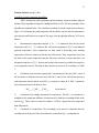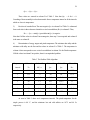
1
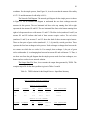
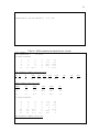
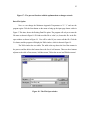
THE HEAT EXCHANGER NETWORK
( THEN )
USER’S MANUAL
and
TUTORIAL
Kedar Telang, F. Carl Knopf and Ralph W. Pike
March 1, 2001
Copyright 2001
Mineral Processing Research Institute
Louisiana State University
Baton Rouge, LA-70803
DISCLAIMER
Mineral Processing(MPRI) makes no warranties, express or implied, including without
limitation the implied warranties of merchantability and fitness for particular purpose, regarding
the MPRI software. MPRI does not warrant, guarantee or make any representation regarding
the use or the results of the use of the MPRI software in terms of its correctness, accuracy,
reliability, currentness or otherwise. The entire risk as to the results and performance of the
MPRI software is assumed by you.
In no event will MPRI, its director, officers, employees or agents be liable to you for
any consequential, incidental or indirect damages (including damage for loss of business profits,
business interruption, loss of business information, and the like) arising out of the use or inability
to use the MPRI software even if MPRI has been advised of the possibility of such damages.
TABLE OF CONTENTS
I
INTRODUCTION
1
Installation
II
III
1
TUTORIAL SESSION
2
Process Example
2
Pinch Analysis
4
USING “ THEN ”
7
Introduction
7
Interactive Data Entry Option
8
Output Menu
16
Evaluation of results
17
Grand composite curve
17
Network grid diagram
Output data file
18
18
Flowsheet for the improved process
Data file option
IV
INPUT DATA REQUIREMENTS
21
22
26
Number of hot streams
26
Number of cold streams
26
Stream names
26
Stream flowrates
26
Units
27
Stream heat capacity
27
Stream source temperature
27
Stream target temperature
27
Minimum approach temperature
27
Stream heat transfer film coefficient
28
V
RESULTS FROM THEN
29
VI
ADDITIONAL INFORMATION
34
Grand composite curve
34
Solution method
35
Program limits
37
General information
37
REFERENCES
39
INDEX
40
LIST OF FIGURES
Figure 1
Flowsheet for a simple process
2
Figure 2a
Temperature profiles for streams
5
Figure 2b
Composite curves for streams
5
Figure 3
Combined composite curve
6
Figure 4
The main window
7
Figure 5
The input option page
8
Figure 6
The interactive data page
9
Figure 7
The hot stream page
10
Figure 8
The cold stream page
11
Figure 9
The incorrect data message
11
Figure 10
The escape option
12
Figure 11
The save as window
12
Figure 12
The execution window
13
Figure 13
The output menu window
14
Figure 14
The grand composite curve
14
Figure 15
The network grid diagram
15
Figure 16
The output data window
15
Figure 17
The process flowsheet with the optimum heat exchanger network
22
Figure 18
The file open window
23
Figure 19
The edit window
23
Figure 20
The add a stream window
24
Figure 21
The network grid diagram with loop path
33
LIST OF TABLES
Table 1Process streams data
3
Table 2a
THEN solution for simple process - Input data summary
18
Table 2b
THEN solution for simple process - Results
19
Table 3The Problem Table Algorithm
36
1
I
INTRODUCTION
THEN is a heat exchanger network synthesis program that was developed by Professor
Knopf at Louisiana State University (Knopf ,1989). It integrates the networks of heat
exchangers, boilers, condensers and furnaces for best energy utilization. It uses pinch
technology as the basis for designing a network.
The Additional Information section provides more details on the types of problems
that can be solved using THEN. This includes the limits on the number and type of streams and
heat exchangers.
The program was originally developed on an IBM mainframe machine, and
subsequently moved to the PC. The PC version has been revised once. Enhancements over the
earlier version include a modified solution algorithm that is able to solve certain problems that
the original version could not solve, ability to name process streams and the calculation of heat
exchanger areas from user supplied film coefficient data.
A graphical interface was added recently to make the program more efficient and
attractive. Microsoft Visual Basic 5.0 was chosen for this purpose. The interface uses
interactive windows to handle the input-output operations in a user-friendly manner.
Installation
The Heat Exchanger Network (THEN) program must be installed under Windows 95
or Windows NT. The procedure to install the program is described as following:
1)
Insert disk 1 in drive a (or b) and run the “setup.exe” program.
2)
The default destination directory is “C:\then” into which the THEN program will be
copied when the setup program is run.
3)
Run the program “Then.exe” in the installation directory.
2
II
TUTORIAL SESSION
Process Example
THEN uses Pinch Analysis for the optimum design of heat exchanger network. It
employs three concepts: the composite curves, the grid diagram of process stream and the pinch
point; and these are applied to minimize the energy use in the process. This program takes the
necessary streams information from the user and decides the best arrangement of heat
exchangers, heaters and coolers so that the amount of utilities needed such as cooling water and
steam is minimized. It plots the Grand Composite Curve (GCC), which shows the enthalpy of
the process streams as a function of temperature. It also shows the heat exchanger network
design in a graphical form as the network grid diagram for visualization of the network
configuration.
FEED 1 (C1)
REACTOR 1
PRODUCTS 1 (H1)
125.0
20.0
150.0
Heater
60.0
Cooler
FEED 2 (C2)
REACTOR 2
25.0
100.0
Heater
90.0
PRODUCTS 2 (H2)
OFF GAS
60.0
Cooler
Separator
60.0
60.0
Figure 1: Flowsheet for a Simple Process
The best way to understand the concepts of pinch technology and the use of THEN is
to consider a process scheme encountered in the chemical industry. The flowsheet in Figure 1
3
shows a simple process which involves two reactors and a separation unit. Our objective is to
minimize the use of cooling water and steam by application of THEN and determine a better
design for the process.
In Figure 1, there are two hot streams and two cold streams that will be analyzed using
THEN. The feed to the Reactor1 has to be heated from 20.0 °C to 125.0 °C, and the feed to
Reactor2 has to be heated from 25.0 °C to 100.0 °C. These are the cold streams that increase
in temperature. Product from Reactor1 needs to be cooled from 150.0 °C to 60.0 °C whereas
the product out of Reactor2 has to be cooled from 90.0 °C to 60.0 °C. These are the two hot
streams that decrease in temperature.
Now that we have defined the problem and identified the hot and cold streams, we
need to know the flowrate, heat capacities and the film heat transfer coefficients for each of
these streams. All of this data for the above process is given in the Table 1 below. The names in
the brackets will be used as the stream identifiers in the program. For each stream, you must
enter a unique name.
Table 1 Process Stream Data
Film Heat Transfer
Stream Name
Flowrate (kg/s)
Heat Capacity (J/kg-°C)
Products1 (H1)
1.0
2.0
1000.0
Products2 (H2)
1.0
8.0
1000.0
Feed1 (C1)
1.0
2.5
500.0
Feed2 (C2)
1.0
3.0
500.0
Coefficient (J/m2-s-°C)
THEN also requires a Minimum Approach Temperature. This is the closest approach
temperature allowed between two streams exchanging heat. There is no fixed recommended
value for this temperature difference, and optimum values depend on the process. For this
process, we have chosen a Minimum Approach Temperature of 20 °C.
4
The section on Input Data Requirements in this manual describes the information
required by the program. Now we have all the necessary data, and we are ready to use THEN
for this problem. But before that, lets try to understand what Pinch Analysis means and how
THEN will use pinch analysis to solve this problem.
Pinch Analysis (Shenoy, 1995)
This is a technique for evaluating the heat flows in any heat exchanger network. The
process streams are first divided into hot and cold streams. For each stream, the enthalpytemperature diagram is drawn. This is shown in Figure 2(a) for the process described in Figure
1. Then, all of the hot streams are then combined to generate the Hot Composite Curve and all
the cold streams are combined to give Cold Composite Curve. These composite curves are
shown in Figure 2(b). This combination is done by summing up the mass heat capacity values
of all streams of the same kind (hot or cold) within each temperature interval. The limits of the
temperature interval correspond to the inlet and outlet temperatures of the streams.
The hot and cold composite curves provide a comprehensive picture of the heat supply
and heat demand for the process over the entire temperature range. In essence, all process
streams may be combined and visualized as a single hot stream and a single cold stream in
counterflow with a piecewise variation in the mass heat capacity. When the two curves are
drawn together, the combined composite curve is obtained. This is shown in Figure 3. In the
combined composite curve, the minimum approach temperature determines the relative position
of the two curves. As shown in Figure 3, the minimum approach temperature is 20 °C.
The point at which the two curves come closest is called the Pinch Point, and the
corresponding temperature is called the Pinch temperature ()Tmin). The pinch point divides the
process into two thermodynamically separate regions. The pinch point is shown by arrows in
Figure 3.
Below the pinch, there is a heat surplus and only utility cooling is required. Any utility
heating supplied to the process below the pinch temperature cannot be absorbed and will be
rejected by the process to the cooling utility, increasing the amount of cooling utility required.
5
Similarly, the problem above the pinch requires only utility heating and no utility cooling. Any
utility cooling above the pinch temperature has to be made up by additional utility heating.
6
160
160
120
120
H1
T (°C)
C1
80
T (°C) 80
C2
H2
40
40
0
0
0
100
200
300
400
500
0
100
200
Q (W)
300
400
500
Q (W)
Figure 2(a) : The temperature profiles of hot streams (on the left side) and cold streams (on the
right side) for the simple process.
160
160
120
120
T (°C) 80
T (°C) 80
C1+C2
H1+H2
40
40
0
0
0
100
200
300
Q (W)
400
500
0
100
200
300
400
Q (W)
Figure 2(b) : The composite curves for hot streams (on the left side) and cold streams (on the
right side) for the simple process.
500
7
160
120
T (°C)
Cold
Hot
80
)T min = 20
40
0
0
100
200
300
400
500
600
Q (W)
Figure 3 : The combined composite curve.
Once, the problem is divided into two sub-problems, a problem above the pinch and a
problem below the pinch, each one is solved separately, beginning at the pinch temperature. In
each case, the most constrained hot stream (the one with the lowest temperature) is considered
for heat exchange with the most constrained cold stream (the one with the highest temperature).
If heat exchange is thermodynamically possible between these two streams, it is counted as a
match. If heat exchange is not possible, the next most constrained stream is chosen for
consideration. This process is continued until a match is found. The amount of heat transfer is
equal to the maximum heat transfer thermodynamically possible. The process is repeated for all
the streams. Based on the matches made, the new heat exchanger network configuration is
decided. One of the rules used to ensure that the best heat exchanger configuration is found is
that heat transfer must not cross the pinch temperature by process to process heat transfer or
inappropriate use of utilities. This rule is both necessary and sufficient to ensure the best
configuration as long as all of the heat exchangers have a temperature difference smaller than the
minimum approach temperature. (Smith,1995)
Thus, THEN takes the necessary stream data for the process and applies the basic
concepts of pinch technology to determine the optimum process design. Having understood
8
how THEN works, now we can use the program to determine the best configuration for the
heat exchanger network.
9
III
Using “THEN”
Introduction
Upon running THEN, the first window presented to the user is the main window with
the menu. This is shown in Figure 4 below.
Figure 4 : The Main Window
The welcome message at the center tells the user about the options available in the
menu. When the user begins a task by choosing the Start button, it automatically becomes
dimmed and is unavailable till the task is over. Note that the main window acts as the container
for the entire application, and the menu will be accessible to the user at all times. Also, at any
stage, the Exit button can be clicked to end the program.
10
When the user clicks the start button, the Input option page is presented. This is shown
in Figure 5 below. Here, the user can choose either the Data File option or the Interactive Data
entry option.
Interactive Data Entry Option:
This option is recommended when the data is being entered for the first time and does
not exist in a file. So, we will select the Interactive option for our problem here. The use of the
Data-File option is explained later.
Figure 5 : The Input Option Page
On choosing the interactive option, a message is flashed on the screen. This informs the
user that the data can be entered in any consistent set of units. So, we will be entering all the
data in kg-m-°C-sec system.
The next page of this option is shown in Figure 6, and the user is asked to enter the
number of hot streams, number of cold streams and the minimum approach temperature. We
11
enter the values as shown in the Figure 6 using the data in Table 1. After this, the user can either
move forward by clicking the YES button or go back to the input page by pressing CANCEL.
Figure 6 : The Interactive Data Page
The next page is shown in Figure 7, and it is the Hot Stream page. The stream number
in the topmost label shows the current stream for which data is being entered. The user has to
enter the various data items e.g. stream name, flow-rates etc. We now enter all the data for
stream H1 as shown. This data is given in Table 1.
After this, the user can go to the next stream by pressing the Next Stream button and
enter data for that stream. Also, the user can go back to any previous stream by pressing the
Previous Stream button. When the last stream is reached, the DONE button becomes enabled.
Clicking this button takes the user to the next page to enter the data for the cold streams as
shown in Figure 8.
12
Figure 7 : The Hot Stream Page
If the data entered is non-numeric or any of the data fields has been left blank, the
program displays the message ‘Incorrect Data. Please enter again’ as shown in Figure 9. At any
stage, the user can press ESCAPE to quit the data entry part. A message appears in a window
as shown in Figure 10. It warns the user that the data entered has not been saved. The user can
either press RESUME to continue data entry or press RESTART to lose data and start again or
press EXIT to end the task.
13
Figure 8 : Cold Stream Page
Figure 9 : The ‘Incorrect Data’ Message
14
Figure 10 : The Escape Option
Figure 11 : The ‘ Save As ’ Window
15
The Cold Stream page shown in Figure 8 is very similar to the Hot Stream Page. The
user can move forward and backward in the streams using ‘Next stream’ and ‘Previous
Stream’ button. At any stage, the ‘Go Back to Hot Streams’ button can be clicked to go to the
window for hot streams data and make changes.
When the user has accurately entered all the data, the ‘Done’ button on the Cold
Streams page should be clicked. After this, the user can not make further changes.
The program then asks the user to save the data in a file by displaying the ‘Save As’
window which is shown in Figure 11. Saving the data is absolutely necessary so that it can be
used in the subsequent runs. Lets save this data in the file ‘a.dat’ in the 'Then' directory.
At this stage, all of the data required to run the THEN program is available in the datafile. The Visual Basic program assembles this data and is ready to call ‘THEN’ to run the
program with the data-file.
The Execution Window shown in Figure 12 appears on the screen asking whether the
user is ready to start executing the program. At this stage, the user clicks on the YES button,
and the program is run. However, if the user realizes that he has made some mistakes in the
data, he can quit the application by clicking the EXIT button. Since the data has been saved in a
file, the user can start another task and edit the file using the data-file option explained later.
Choosing the YES button on the Execution window button will run the THEN program,
and an Output Menu Window will appear on the screen as shown in Figure 13.
Figure 12 : The Execution Window
16
Figure 13 : The Output Menu Window
Figure 14 : The Grand Composite Curve
17
The Output Menu
Clicking the first button ‘View and save the GCC’ on the 'Output Menu Window'
displays the 'Grand Composite Curve' on the screen. This is shown in Figure 14. It is a plot of
enthalpy flows in the system versus temperature. The menu bar at the top of the diagram
provides options for viewing and printing the diagram. Clicking the 'View' button displays the
commands to turn off the grid and show the data points. The 'Print Options' button can be used
to set the number of copies and change the orientation. Clicking the 'Print' button will print the
diagram to the default system printer. Click the 'Save' button to save the diagram in 'Windows
Metafile' format. The 'Help' button will display a brief description about the Grand Composite
Curve. Closing the window brings the user back to the 'Output Menu Window'.
The second button ‘View and save the Grid Diagram’ on the 'Output Menu Window'
displays the 'Network Grid Diagram'. This is shown in Figure 15. It is a graphical representation
of the network solution designed by the program. It shows the arrangement of heat exchangers,
heaters and coolers in the system. Red lines going from left to right represent hot streams and
blue lines going from right to left represent cold streams. A red circle on a blue line means a
heater and a blue circle on a red line is a cooler. Green circles joined by a vertical green line
represent a heat exchanger between the streams on which the two circles lie.
The network grid diagram offers a very convenient way of understanding the solution
network. Clicking on a unit in the diagram displays a small box which shows all the necessary
information for that unit. For example, clicking on a green circle will display the relevant
information for the heat exchanger that it represents. This information includes the names of the
hot and cold streams flowing through it, the heat exchange load of the exchanger and its area.
Clicking on a heater or a cooler will show the name of the stream flowing through it and its heat
load. Similarly, clicking on a horizontal line will display the temperature, mass flowrate and
average heat capacity of that stream. In Figure 15, the heat exchanger with index 1 has been
selected by clicking, and the box at the bottom right side is showing the information for that heat
exchanger.
18
Figure 15 : The Network Grid Diagram
19
Figure 16 : The Output Data Window
Information about the grid diagram can be obtained as online help by clicking the 'Help'
button in the menu bar at the top of the diagram. Other buttons in the menu bar are to set the
view and print options. The 'Zoom' button allows the user to change the zoom of the diagram.
The 'View' button can be used to display the printer lines. The 'Print' button will open the printer
dialog box and print the diagram to the selected printer. Closing the window will take the user
back to the 'Output Menu Window' shown in Figure 13.
The third button, the ‘View and save the Output Data’ button shows the output text file
in a window (Figure 16). Using horizontal and vertical scroll bars, the user can see the entire
output text. The 'Print' button at the top of the window prints output file to the default printer.
On clicking the ‘Save’ button, the program opens the 'Save as' window and requests the user to
specify the filename. Let us save the output as file 'out.dat' in the directory 'Then'. Click the
'Close' button to go back to the Output Menu window.
More information on the method of solution and the grand composite curve is given in
the Additional Information section of this manual.
Clicking the 'Exit' button will end the current task and take the user back to the main
window shown in Figure 4. Now the user can click the START option in the menu to start
another task or click the Exit button to quit the application.
Using the results from THEN
The Grand Composite Curve (GCC): The GCC for the simple process is shown in
Figure 14. It is a plot of temperature on Y-axis versus the enthalpy flow on X axis. If the curve
touches the temperature-axis at 0.0 enthalpy, it is a pinched process, and the temperature
corresponding to that point is the pinch temperature. In Figure 14, the GCC meets the
temperature axis at 80. Hence, the pinch temperature for this process is 80 °C.
Also, the GCC can be used to determine the minimum amount of hot and cold utilities
needed by the process. To find the amount of hot utility required, locate the topmost point of the
curve and read its X coordinate which is equal to the amount of hot utility. Similarly, to get the
amount of cold utility required, locate the bottommost point of the curve and read its X
20
coordinate. For the simple process, from Figure 14, it can be seen that the amount of hot utility
is 107.5 J/s and the amount of cold utility is 40 J/s.
The Network Grid Diagram: The network grid diagram for the simple process is shown
in Figure 15. Let us examine this diagram to understand the new heat exchanger network
structure for this process. The two horizontal red lines at the top running from left to right
represent the hot streams H1 and H2. The two horizontal blue lines at the bottom running from
right to left represent the two cold streams C1 and C2. The blue circles (numbered 1 and 2) on
streams H1 and H2 indicate that both of these streams require coolers. The red circles
(numbered 1 and 2) on streams C1 and C2 show that both of these streams require heaters.
There are four pairs of green circles (numbered 1, 2, 3, 4) joined by vertical green lines. These
represent the four heat exchangers in the process. Each exchanger exchanges heat between the
two streams on which the two circles lie. For example, heat exchanger 1 (the pair of green
circles with number 1) is exchanging heat between hot stream H1 and cold stream C1. Thus, it
can been seen from the grid diagram that the simple process needs four heat exchangers, two
heaters and two coolers in new network solution.
The Output Data File: Now, let us examine the output data generated by THEN. The
complete output file for the above problem is given in Tables 2 a and b.
Table 2a THEN solution for the Simple Process - Input Data Summary
HEAT EXCHANGER NETWORK SYNTHESIS
DETAILS OF HOT STREAMS
ST NAME
FLOWRATE
MCP
INLET T
OUTLET T
FILM COEFFICIENT
H1
1.0
2.0
150.0
60.0
1000.0
H2
1.0
8.0
90.0
60.0
1000.0
DETAILS OF COLD STREAMS
ST NAME
C1
FLOWRATE
MCP
INLET T
OUTLET T
1.0
2.5
20.0
125.0
FILM COEFFICIENT
500.0
21
C2
1.0
3.0
25.0
MINIMUM DELTA T FOR THE MATCHES IS
100.0
20.00
500.0
DEG
Table 2b THEN solution for the Simple Process - Results
PINCH LOCATED
PINCH TEMPERATURE =
ALL STRMS EXHAUSTED
.0
.0
.0
.0
1.0
.0
.0
.0
.0
2.0
80.000000
.0
.0
.0
.0
140.0
.0
.0
.0
.0
.0
2.0
3.0
80.0
90.0
.0
1.0
2.5
128.0
17.5
120.0
HEAT EXCHANGER SUMMARY ABOVE THE PINCH
HEX
CS
HS
HEAT
THIN
THOUT
TCIN
1.
C1
H1
120.0
150.0
90.0
70.0
TCOUT
CPH
118.0
2.0
HEATER SUMMARY ABOVE THE PINCH
HEATER
CNO
HEAT
TCIN
TCOUT
1.0
1.0
17.5
118.0
125.0
2.5
2.0
2.0
90.0
70.0
100.0
3.0
ALL STRMS EXHAUSTED
.0
.0
.0
.0
2.0
2.0
1.0
.0
.0
.0
.0
5.0
3.0
2.0
.0
.0
.0
.0
55.0
50.0
57.5
.0
.0
.0
.0
.0
.0
15.0
HEAT EXCHANGER SUMMARY BELOW PINCH
2.0
3.0
35.0
.0
.0
90.0
45.0
1.0
2.5
30.0
.0
125.0
.0
.0
CPC
CPC
2.5
AREA
.014
22
HEX
CS
HS
2.
C2
H2
3.
C1
4.
C2
HEAT
THIN
THOUT
TCIN
TCOUT
CPH
CPC
AREA
90.0
90.0
60.0
40.0
70.0
3.0
3.0
.014
H2
125.0
90.0
65.0
20.0
70.0
5.0
2.5
.012
H1
45.0
90.0
67.5
25.0
40.0
2.0
3.0
.003
COOLER SUMMARY BELOW THE PINCH
COOLER
CNO
1.0
1.0
15.0
2.0
2.0
25.0
LOOP#
HEAT
THIN
THOUT
CPH
67.5
60.0
2.0
63.1
60.0
8.0
HEAT EXCHANGERS INVOLVED
1
4
1
2
3
THE MINIMUM HOT UTILITY REQUIREMENT IS:
107.500000
THE MINIMUM COLD UTILITY REQUIREMENT IS:
40.000000
The following discussion is be for the most relevant information for the simple process.
A complete discussion is presented in the section Results from THEN later in the manual.
Table 2a simply lists a summary of the input information entered by the user. This
consists of the data for hot and cold streams followed by the specified minimum approach
temperature for the matches.
Table 2b lists the results for the simple process. The first two lines of output mean that
the given problem was a pinched problem and that the pinch temperature was found to be 80
°C. (For more information on these terms, see the section Results from THEN).
This is followed by a matrix of values which is the solution array generated by THEN
for the problem above the pinch. These values can help in understanding the matches made by
the program to arrive at the solution. However, the most important part of the output is the Heat
Exchangers, Heaters and Coolers summary tables, which follow.
The heat exchanger summary above the pinch shows that there should be a heat
exchanger between streams H1 and C1. The heat transfer rate will be 120 J/s. Also, it gives the
inlet and outlet temperatures for both the streams. Note that the area of the heat exchanger
(0.014 m2) has been calculated using the film heat transfer coefficient supplied in the data.
23
Next comes the heater summary above the pinch. It shows that we need two heaters in
the system, one for each cold stream. The heat load for the heater on the stream C1 is 17.5 J/s.
C1 enters the heater at 118 °C and leaves at 125 °C. Similarly, the other heater has a load of
90 J/s and heats the stream C2 from 70 °C to 100 °C.
After this comes another solution array for the problem below the pinch. The Heat
Exchangers summary below the pinch is given next, and it has three heat exchangers between
streams C2-H2, C1-H2 and C2-H1. Then, the cooler summary follows and shows that two
coolers, one for each hot stream are needed.
Next comes the information about the loops identified in the network. A loop is any
path in the heat exchanger network that starts at some point and returns to the same
point. For the simple process, there is only one loop in the network, and it involves all of the
four heat exchangers which are needed for this process.
Finally, the last two lines of output give the minimum hot and cold utilities needed for this
process. Thus, for this simple process, 107.5 J of external heat needs to be supplied and 40.0 J
of heat needs to be removed.
Note that just above the printout of the two solution arrays is a message which says if all
the streams were exhausted or not. If the message is ‘all streams exhausted’ for both above the
pinch and below the pinch problems, THEN has successfully generated the heat exchanger
network. If the message is ‘Error- not all streams exhausted’, THEN has failed to solve the
problem. In this case, the order of the streams in the input data should be changed. For
example, the data for stream H2 should be entered before stream H1. The program uses a
solution method that is sensitive to the order in which the stream data is entered.
To summarize, the simple process has a pinch point at 80 °C, and it needs 4 heat
exchangers, 2 heaters and 2 coolers for maximum energy utilization. The minimum amount of hot
utility is 107.5 J/s and the minimum amount of cold utility is 40 J/s.
Flowsheet for the Improved Simple Process
24
Using the above results, let us build a process flowsheet which incorporates the new
heat exchanger network design. The network grid diagram generated by THEN for this process
(shown in Figure 15) can be of great help in this effort.
In the network grid diagram, we select a particular stream and follow its path in the
network. We start with its source and follow it until it reaches its target temperature. Along this
path, the stream flows through various heat exchangers, heaters and coolers. For example, we
select the hot stream H1 and follow its path. We see that it flows through heat exchanger 1 and
then passes through heat exchanger 4 and then finally, it is cooled down to its target temperature
by cooler1. We repeat this exercise for all the streams. The inlet and outlet temperatures for
each of the heat exchangers, heaters and coolers can be obtained either from the grid diagram
by simply clicking that unit or can be read from the output data file. All these heat exchangers,
heaters and coolers are now included in the process flowsheet at the appropriate places. The
new process flowsheet thus obtained features the optimum heat exchanger network. The new
flowsheet for the simple process is given in Figure 17.
PRODUCTS 1
FEED 1
E1
E3
Reactor 1
70 °C
20 °C
118 °C
150 °C
125 °C
Heater 1
90 °C
FEED 2
E4
90 °C
E2
70 °C
40 °C
25 °C
Reactor 2
100 °C
PRODUCTS 2
Heater 2
65 °C
67.5 °C
60 °C
60 °C
OFF GAS
63.1 °C
Cooler 1
60 °C
Cooler 2
60 °C
60 °C
25
Figure 17 : The process flowsheet with the optimum heat exchanger network
Data-File Option
Now we can change the Minimum Approach Temperature to 25 °C and run the
program again. Click the Start button on the menu to bring up the input page shown earlier in
Figure 5. This time, choose the Existing Data File option. The program will ask you to enter the
file name as shown in Figure 18. We had saved the file as ‘a.dat’; so, choose this file in the fileopen window as shown in Figure 18. You will be asked if you want to edit the file. Click the
Yes button, and the program will display the 'Edit' window, which is shown in Figure 19.
The 'Edit' window has two tables. The table at the top shows the list of hot streams in
the process and the table at the bottom shows the list of cold streams. There are three buttons
adjacent to the table of hot streams; 'Add hot stream', 'Delete hot stream' and 'Edit hot stream'.
Figure 18 : The File-Open window
26
Figure 19: The Edit window
27
Figure 20 : 'Add a stream' window
To add a hot stream, click the 'Add hot stream' button. A small window will be shown
to enter the data for the new hot stream. This is shown in Figure 20. After entering all the
necessary data, click the 'Done' button. To go back to the 'Edit' window without adding a
stream, click the 'Cancel' button. To delete a stream from the hot streams table, select that
stream in the table by clicking the mouse pointer on that row and then click the 'Delete hot
stream' button. The row will be deleted from the table. To change the data for a particular hot
stream, select that stream in the table and click the 'Edit hot stream' button. A small window
similar to the window in Figure 20 is displayed. Enter the new data values for the selected
stream and click the 'Done' button. The values for that stream in the table will be changed.
Similar to the buttons for the hot streams, there are three buttons for the cold streams;
'Add cold stream', 'Delete cold stream' and 'Edit cold stream'. These buttons can be used to
add a cold stream, delete a cold stream and edit a cold stream in the cold streams table in
exactly the same manner as the buttons for the hot streams.
At the bottom of the 'Edit' window, the minimum approach temperature is shown. We
can change this value to from 20 to 25.
After all the changes are made, the 'Finish' button on the edit window should be clicked.
The user is now asked if the changes made in the edit window should be accepted.
Click 'Yes' to accept the changes. This modified data will now be used for the next run. The
user is further asked if the new data is to be saved to a file. This time, save the data with a
different filename of your choice.
THEN now shows the same Execution window shown in Figure 12. Run the program
and analyze the output just as we did for approach temperature of 20 °C. This is left as an
exercise for the reader.
28
IV
INPUT DATA REQUIREMENTS
The data required for a THEN run is explained below.( Knopf, 1989 )
Number of Hot Streams
This is the total number of hot streams in the problem. A hot stream is defined as a
stream that has to be reduced in temperature. By definition, a hot stream is a source of heat.
This heat may be used to heat other cold streams or may have to discarded in a cooling utility
such as air, cooling water or a refrigeration system.
Number of Cold Streams
This is the total number of cold streams in the problem. A cold stream is defined as a
stream that has to be increased in temperature. By definition, a cold stream requires heat and is
a source of cooling. This heat may come from other hot streams or from a hot utility such as
steam, a fired heater or a heat transfer fluid such as DOWTHERM. An alternate way of
looking at this is that the cooling capacity of a cold stream may be used to cool other hot
streams or may have to be discarded in a hot utility. This definition is more useful in cases
where the cost of cooling may be significantly higher than the cost of heating, such as in
refrigeration cycles.
Stream Names
Each stream can be given a name of up to 12 characters long for ease of identification.
Stream Flowrates
The flowrate of each stream is required to compute the total heating or cooling required
by the stream and to compute its heating and cooling capacity. The heating or cooling capacity
of a stream is the change in the temperature of the stream when it absorbs one unit of heat. This
is also the product of the stream flowrate and its specific heat. Note that streams with a very
large heating or cooling capacity may require a small amount of total heating or cooling if the
temperature range they span is small, and streams with small heating or cooling capacities can
require a large amount of heat if they span a large temperature range.
29
Units
THEN does not require any particular set of units. However, care must be taken to
provide the input in a consistent set of units.
Stream Heat Capacities
These are required to compute the stream heating and cooling capacity as explained
under stream flowrates. The units used must be consistent with the units used for the flowrates
and temperatures.
Stream Source Temperatures
This is the temperature at which the stream is available from the plant or process before
it undergoes any heat exchange.
Typically, this is the battery limit temperature, or the
temperature at which a stream originates from process equipment such as a reactor or
distillation column.
Stream Target Temperatures
This is the temperature at which the stream is desired after all heat exchange has been
completed, including heating by hot utilities such as steam or fired heaters, or cooling by cold
utilities such as water or air. Typically, this is also a battery limit condition or the temperature at
which a stream must enter process equipment such as a reactor or a distillation column.
Minimum Approach Temperature
This is the closest approach temperature that is allowable between two streams
exchanging heat. There is no fixed number that can be uniformly recommended. Typically, in
crude distillation units, a value of 30 to 50 deg F is reasonable, whereas in refrigeration cycles, a
value of 10 to 15 deg F is reasonable. However, the optimum value of this parameter is
significantly affected by the relative costs of energy and heat exchange area, and this is the
primary parameter that has to be optimized in any pinch design.
The minimum approach temperature selected affects both the capital costs and the
operating costs. Selecting a low value means that hot streams can approach the temperature of
the cold streams more closely. The cold stream thus absorbs more heat from the hot stream.
This reduces the utility heating required for the cold stream and also the utility cooling required
for the hot stream, as the hot stream exits at a lower temperature after heat exchange with the
30
cold stream. This reduces the operating costs by lowering the utility costs, but it also increases
the capital costs, since the lower approach temperature between the hot and cold streams
reduces the Log Mean Temperature Difference (LMTD) in the heat exchanger. The lowered
driving force and higher duty of individual heat exchangers results in larger heat exchanger areas
being required, which increases capital costs. Similarly, a large value of the minimum approach
temperature results in lower capital costs and higher utility (operating) costs.
Stream Heat Transfer Film Coefficients
The overall heat transfer coefficient is used to estimate the area required for each heat
exchanger generated by THEN. Assuming a counter-current flow in the heat exchanger, the
following equation is used.
Q = U A ∆Tlm
(1)
The overall coefficient is computed from the film heat transfer coefficients using the
following approximate equation.
1/U
= 1 / hc + 1 / hh
(2)
where U is the heat exchanger overall heat transfer coefficient, hc is the cold stream coefficient
and hh is the hot stream coefficient.
The exchanger area is given by the following equation
Area = Q / ( U x ∆Tlm)
(3)
where Q is the exchanger duty ( m Cp ∆T for no phase change) and ∆Tlm is the log mean
temperature difference in the exchanger [ ( ∆T1 - ∆T2 ) / ln ( ∆T1 / ∆T2) ].
Care must be taken to ensure the film coefficients are entered in units consistent with the
units used for the flowrates, heat capacities and temperatures.
31
V
RESULTS FROM THEN
The results from THEN consist of an echo of the input data, details of the heat exchange
matches made, a summary of the loops detected in the network, the total hot and cold utility
required as illustrated in Table 2b. THEN also shows the Grand Composite Curve and a
graphical display of the Network Grid Diagram.
Before explaining the output file, it is necessary to provide some background on pinch
technology to explain some of the terms that will be encountered.
Pinch analysis is a technique for evaluating the heat flows in any heat exchange
network. It is used to determine the pinch temperature. The pinch temperature is a temperature
determined from the stream data and the approach temperature. It is used to separate the
problem into two sub problems, called the problem above the pinch and the problem below the
pinch.
The problem above the pinch is always in heat deficit, and the problem below the pinch
is always in heat surplus. The problem above the pinch requires only utility heating and no utility
cooling, and the problem below the pinch requires only utility cooling and no utility heating. Any
utility heating supplied to the process below the pinch temperature cannot be absorbed and will
be rejected by the process to the cooling utility, increasing the amount of cooling utility required.
Similarly, the problem above the pinch requires only utility heating and no utility cooling. Any
utility cooling above the pinch temperature has to be made up by additional utility heating.
Some processes require no utility cooling at all, only utility heating. Such a process is
said to lie above the pinch. Other processes require no utility heat at all, only utility cooling.
These processes are said to lie below the pinch. Problems that are entirely above the pinch or
entirely below the pinch are called unpinched problems.
The results from solution of THEN are given in Tables 2a and 2b for the simple
process. This is typical of the output for a general problem. The first section of the output file
consists of an echo of the hot stream data followed by an echo of the cold stream data and the
minimum approach temperature to be used. This is followed by a statement that the problem is a
pinched problem or an unpinched problem. For a pinched problem, the statement 'Pinch
32
located' is given and the pinch temperature is reported as shown in Table 2b. Following this
pinch temperature is the solution array for the problem above the pinch temperature. Just above
the solution array, a message states whether all streams were exhausted or not exhausted.
THEN has successfully generated a heat exchanger network for the problem above the pinch if
the message 'all streams exhausted' appears after the pinch temperature as shown in Table 2b. If
the message says 'error-all streams not exhausted', THEN was unsuccessful in generating a
network above the pinch.
The solution array above the pinch is a matrix that represents the streams above the
pinch and the heat exchange matches made between them. The elements of the first four rows in
the first four columns of this array are always zero. Hot streams are represented in the rows of
this array, beginning from row five, and cold streams are represented in the columns of this
array, beginning from column five. For example, the first element of the fifth row is 1. This
means that the fifth row represents hot stream H1 because H1 is the first hot stream in the
order of hot streams for the input data. Similarly, the first element of the fifth column of the
matrix is 2. This means that the fifth column represents stream C2 because stream C2 appears
second in the input order of cold streams. The second element of a row or a column shows the
product of mass flowrate and heat capacity for the stream that it represents. For example, the
fifth column represents the stream C2. The second element of that column is 3 which is equal
to the product of the mass flowrate and heat capacity of stream C2. The intersection of a row
and column gives the amount of heat exchange between the hot stream and the cold stream they
represent. For example, intersection of fifth row and fifth column is 120. This means that there is
an heat exchanger between stream H1 and stream C1. This exchanger is placed above the
pinch and the heat exchange load of this exchanger is 120 J/s.
For the problem above the pinch, the message 'all streams exhausted' indicates that the
cooling requirements of all the hot streams above the pinch have been met, and all the hot
streams are exhausted. For the problem below the pinch, the message 'all streams exhausted'
indicates that heating requirements of all the cold streams have been met, and all the cold
streams are exhausted as illustrated in Table 2b.
33
Note that ‘THEN’ has successfully generated a solution only when the message "all
streams exhausted" appears for the problem above the pinch as well as the problem below the
pinch.
The solution array is followed by the heat exchanger summary above the pinch and it
lists the heat exchangers and heaters used in the solution for the problem above the pinch. The
heat exchanger summary lists the heat exchanger number (HEX), the name of the hot stream
and the cold stream exchanging heat (HS and CS respectively), the exchanger duty (HEAT),
the hot and cold inlet and outlet temperatures (THIN, THOUT, TCIN, TCOUT), the product
of the mass flow and specific heat for the hot and cold stream (CPH and CPC), and the
exchanger area (AREA).
The heat exchanger summary is followed by the heater summary. This summary lists the
heater number (HEATER), the stream number of the cold stream flowing through it (CNO), the
heating load of the heater (HEAT), the inlet and outlet temperature of the cold stream flowing
through it (TCIN and TCOUT) and the product of the mass flow and specific heat of the cold
stream (CPC).
Next the information is given for the solution below the pinch. This includes the solution
array, heat exchanger summary and cooler summary for the problem below the pinch. The
description of the information in the solution array and the heat exchanger summary is the same
as the information for solution above the pinch. The cooler summary information is as follows. It
lists the cooler number (COOLER), the stream number of the hot stream flowing through it
(CNO), the cooling load of the cooler (HEAT), the inlet and outlet temperature of the hot
stream flowing through it (THIN and THOUT) and the product of the mass flow and specific
heat of the hot stream (CPH).
Next the information is given for the loops in the system. A loop refers to a closed path
on the heat exchanger network grid diagram formed by a combination of heat exchangers and
streams. For the simple process, there is one loop and it involves heat exchangers 4, 1, 2 and 3
as shown in Table 2b.
Physically, a loop represents those areas of the network where more exchangers have
been used than are theoretically required. For a problem involving n streams, the number of
34
exchangers theoretically required is n-1 according to Shenoy, 1995. However, it is usually not
possible to achieve the desired utility use with this number of exchangers. Since the pinch
method breaks any problem into two sub problems and solves them independently, only the sub
problems are likely to satisfy this rule. The whole problem will have a number of loops equal to
the number of streams that exist both above the pinch and below the pinch.
Loops can be broken by removing one of the exchangers that is a part of it. If one of
the exchangers in the loop lies above the pinch, and the other lies below the pinch, then breaking
the loop will incur an energy penalty equal to the duty of the exchanger that is removed.
However, if the loop lies entirely above the pinch or entirely below the pinch, it may be possible
to readjust the duties of the other exchangers so that there is no energy penalty. The loop
summary provided by THEN is intended to assist in these evaluations by highlighting the loops in
the design generated by THEN. THEN currently does not support these reevaluations of the
network.
The loop summary provided by THEN lists all the exchangers involved in the loop. This
information is used to trace the loop on a grid diagram in the following manner. Start with the
first heat exchanger listed in the loop summary. If this exchanger lies above the pinch, locate the
hot stream flowing through it. If the exchanger lies below the pinch, locate the cold stream
flowing through it. Follow this stream in the direction of its flow until you hit another heat
exchanger. This heat exchanger will be one of the heat exchangers listed in the loop summary.
Now locate the stream flowing through the other end of this heat exchanger and then, follow that
stream in the direction of its flow until you come across another heat exchanger. Continue doing
this until you reach your original starting point. The cyclic trajectory traversed in the network in
this manner constitutes the path of the loop. For the simple process, the network grid diagram
has been redrawn in Figure 21 to show the loop path in a dotted line.
The last two items shown on the output are the total hot utility required and the total
cold utility required. For the simple process, the minimum hot utility required (usually steam) is
107.5 J/s. Of this total, 17.5 J/s has to be supplied at a temperature of at least 125 °C and 90
J/s has to be supplied at a temperature of at least 100 °C. The minimum total cold utility
35
requirement, usually cooling water, is 40 J/s and it has to be supplied below a temperature of 60
°C.
1
H1
4
2
H2
1
2
3
1
C1
2
C2
Heater
Cooler
Heat Exchanger
Loop
Figure 21 : The Network Grid Diagram with the Loop Path
This completes the discussion of the results obtained from THEN. The next section
presents detailed information on the grand composite curve and the solution method used by
THEN.
36
VI
ADDITIONAL INFORMATION
Grand Composite Curve (GCC) :
The grand composite curve is a plot of temperature against the net heating or cooling
requirement. The GCC is a useful way to view the heat flows in a system graphically. The GCC
for the simple process described in the tutorial session of this manual is given in Figure 14.
In a GCC, the temperature is plotted on the y axis and the heating or cooling
requirement on the x axis. The curve begins in the top right corner of the graph and descends
towards the bottom left corner. It may change direction several times. It approaches a leftmost
point and then changes direction and descends towards the bottom right corner. The GCC will
touch the y axis at its leftmost point. The point at which the curve touches the y axis is the pinch
temperature of the problem.
The GCC above the pinch temperature represents the problem above the pinch. To
determine the net hot utility required to heat all the streams in the problem to any temperature
above the pinch temperature, simply read the heat flow requirement at that temperature.
Similarly, the GCC below the pinch temperature represents the problem below the pinch. To
determine the net cooling requirement to bring all the streams to any temperature below the
pinch temperature, read the heat flow at that temperature.
If a part of the GCC has a negative slope (top left to bottom right), there is a heat
surplus in that temperature range. This is true above the pinch as well as below the pinch. The
heat surplus is a result of hot streams giving up more heat in that temperature range than can be
absorbed by the cold streams. Often, condensing streams will cause a large heat surplus
because of the large amount of heat released over a relatively small temperature range.
Similarly, if a part of the GCC has a positive slope (bottom left to top right), there is a
heat deficit caused by the cold streams requiring more heat than is available from the hot
streams in that temperature range. Streams undergoing vaporization will typically cause the
GCC to have a positive slope. Thermodynamically, any heat surplus can be used to meet a heat
deficit at a lower temperature, but not at a higher temperature. This represents the spontaneous
flow of heat from a higher temperature to a lower temperature.
37
Solution Method : (Knopf, 1989)
Calculation of pinch temperature and utilities:
THEN calculates the pinch temperature and the minimum amount of utilities using the
Problem Table Algorithm developed by Linnhoff and Flower(1978). The basic principles of this
algorithm are explained below. The calculations presented are for the simple process shown in
Figure 1. For calculating the pinch temperature and the utilities, only the inlet and temperatures,
heat capacities and flowrates are required. The steps of are the algorithm (Shenoy, 1995) are as
follows.
1)
Determination of temperature intervals: )Tmin / 2 is subtracted from the hot stream
temperatures and )Tmin / 2 is added to the cold stream temperatures ()Tmin is the minimum
approach temperature). These temperatures are then sorted in descending order, omitting
temperatures which are common to both hot and cold streams. These temperatures now form
the limits of the various temperature intervals. This step is necessary to ensure that there is an
adequate driving force of )Tmin between the hot and cold streams for possible heat transfer in
every temperature interval. The limits of these intervals are shown as Tint in column A of Table
3.
2)
Calculation of net mass*heat capacity (MC p) in each interval: The sum of MCp values of
the hot streams is subtracted from the sum of the MC p values of the cold streams present in
each temperature interval and the result MC p,int is entered in column B of Table 3 against the
lower temperature limit of the interval. Thus,
MC p,int = ∑ MC p,c - ∑ MC p,h
3)
for the interval
Calculation of net enthalpy requirement in each interval : The MCp,int in each interval is
multiplied by the temperature difference for that interval to obtain the net enthalpy deficit in the
interval (Qint). These values are entered in column C of Table 3 against the lower temperature
limit of the interval.
4)
Calculation of cascaded heat: The net enthalpy in an interval is subtracted from the
cascaded heat in the previous interval to obtain the cascaded heat (Q cas,i) for that interval.
38
Qcas,i = Qcas,i-1 - Qint,i
These values are entered in column D of Table 3. Note that Qcas,i = 0 for i = 0.
Cascading of heat essentially involves heat transfer from a temperature interval to all the intervals
which are lower in temperature.
5)
Revision of cascaded heat: The most negative Qcas in column D of Table 3 is subtracted
from each value in that column to obtain the revised cascaded heat (Rcas) in column E. Thus,
Rcas,i = Qcas,i - min(Qcas) provided min(Qcas) is negative.
Note that if all the values in column D are nonnegative, then step 5 is not required and column E
is the same as column D.
6)
Determination of energy targets and pinch temperature: The minimum hot utility and the
minimum cold utility are the first and last values in column E of Table 3. The temperature in
column A that corresponds to zero revised cascaded heat in column E is the Pinch temperature.
If all the values in column E are positive, then it is an unpinched problem.
Table 3 The Problem Table Algorithm
Temperature
Column A
Column B
Column C
Column D
Column E
interval
Tint
MC p,int
Qint
Qcas
Rcas
0
140
0
0
0
107.5
1
135
-2
-10
10
117.5
2
110
0.5
12.5
-2.5
105
3
80
3.5
105
-107.5
0
4
50
-4.5
-135
27.5
135
5
35
5.5
82.5
-55
52.5
6
30
2.5
12.5
-67.5
40
As seen in Table 3, there are 6 temperature intervals. The pinch temperature for the
simple process is 80 °C, and the minimum hot and cold utilities are 107.5 and 40 J/s
respectively.
39
Synthesis of optimum heat exchanger network:
THEN breaks the network synthesis problem into two problems-the problem above the
pinch and the problem below the pinch. Each problem is then solved separately, beginning at the
pinch temperature. In each case, the most constrained hot stream is matched with the most
constrained cold stream. If a match cannot be made, the next most constrained hot or cold
stream is chosen. The process is repeated until a match can be made. The amount of heat
transferred is the maximum amount that is thermodynamically feasible (until one stream is
exhausted or the streams are separated by the minimum approach temperature). The streams
are then reevaluated to determine the new most constrained hot stream and most constrained
cold stream, and the process is repeated until all the streams have been exhausted.
The most constrained hot stream is the hot stream with the lowest temperature. If two
or more hot streams have the same temperature, the most constrained hot stream is the stream
with the lowest mCp (mass flow x heat capacity) product above the pinch and the lowest mCp
product below the pinch. For cold streams, the most constrained stream is the stream at the
highest temperature. If two cold streams have the same temperature, the most constrained cold
stream is the stream with the highest mCp product above the pinch and the lowest mCp product
below the pinch.
This method of solution sometimes makes THEN sensitive to the order in which stream
information is entered. If THEN is unable to reach a solution, try changing the order of the
streams in the input data.
Program Limits :
THEN is currently limited to a maximum of 50 hot streams, fifty cold streams and fifty
heat exchangers.
General Information :
THEN was developed as a result of a class project in a graduate class on computer
aided design offered by Dr. Knopf at the Chemical Engineering Department at LSU. It is written
in FORTRAN. It has been tried on a number of problems and been found to solve successfully
in most cases. The types of problems that have been solved range from simple classroom
problems, problems from the literature, and industrial problems covering the petrochemicals,
40
refining, and specialty chemicals industries. However, it has been known to fail in some cases
and it is not guaranteed to work with all problems that are likely to be encountered.
41
REFERENCES
Knopf , F. C., Pethe, Singh, Bhargava, and Dhoopar, 1989. THEN User’s Manual.
Shenoy, U. V., 1995, Heat Exchanger Network Synthesis, Gulf Publishing Company, USA.
Smith, Robin, 1995, Chemical Process Design, McGraw Hill Inc., New York, NY.
Linnhoff, B. and Flower, J.R., 1978, Synthesis of heat exchanger networks, AIChE J., 24(4), p
633-642.
42
INDEX
additional information, 34
pinch point, 4
all streams exhausted, 30
pinch temperature, 4
breaking loops, 32
problem above the pinch, 29
cold composite curve, 4
problem below the pinch, 29
combined composite curve, 4
process flowsheet, 2
constrained cold stream, 35
program limits, 35
constrained hot stream, 35
running THEN, 7
editing a data file, 23, 24
saving input data, 13
enthalpy temperature diagram, 4
solution array, 30
existing data file option, 22
solution method, 35
grand composite curve, 14, 17, 34
stream flowrates, 26
grid diagram, see network grid diagram
stream heat transfer film coefficient,
hot composite curve, 4
stream heats capacity, 27
input data requirements, 26
stream matching, 6
interactive data entry, 8
stream names, 26
interface, 1
stream source temperature, 27
loops, 20, 31
stream target temperature, 27
minimum approach temperature, 27
successful solution, 21
network grid diagram,15, 16, 18
tips for cases where problem is not solved,
number of cold streams, 26
21
number of hot streams, 26
tutorial session, 1
order of stream data,
units, 8, 27
output data, 15, 16, 18, 19
unpinched problem, 29
pinch analysis, 4
utilities, 32
28