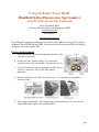
1
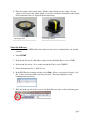
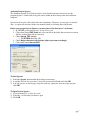
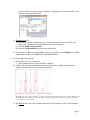
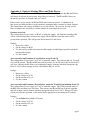
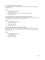
Using the Bruker Tracer III-SD
Handheld X-Ray Fluorescence Spectrometer
using PC Software for Data Collection
Scott A Speakman, Ph.D
Center for Materials Science and Engineering at MIT
[email protected]
617-253-6887
http://prism.mit.edu/xray
This SOP guides you through collecting X-ray Fluorescence (XRF) data using a PC to operate
the Bruker Tracer III-SD handheld XRF. Data can also be collected using a PDA- this mode of
operation is covered in another SOP.
Prepare the Instrument
1. Make sure that the cable from Communications Port to the
computer is connected.
2. If doing low mass elements (Mg to Cl), connect the
vacuum system to the Vacuum Port. Do not turn it on yet.
3. Use the Power Key to turn the instrument on. Turn the key
all the way clockwise. The yellow lamp should
illuminate.
4. Put the desired filter in the filter slot (brass screw). See Appendix A for guidance
choosing a filter.
5. Turn on the vacuum pump. The vacuum gauge should read below 15—if it does not,
contact SEF staff to replace the vacuum window.
pg. 1
6. Place the sample on the sample table. Put the sample shield over the sample. If your
sample is too large for the sample shield, or you need to hold the instrument to the sample
for measurement, then see Appendix B for instructions.
The Sample Table
The Sample Shield
Start the Software
1. Make sure that the XRF unit has been turned on for at least 1 minute before you start the
software.
2. Start S1PXRF
3. In the menu Download > Baud Rate, make sure that the Baud Rate is set to 115200
4. In the menu Download > Port, make sure that the Port is set to COMM 5
5. Select the menu item File > PDZ Preview.
6. In the PDZ Preview dialogue window, select Path. Choose a previously collected *.pdz
file. It does not matter which *.pdz file you select. This step configures several
communication parameters.
7. If the dot in the top left of the screen is red, then click on it once so that it will turn green.
pg. 2
8. Select the menu item Setup > Instrument Setup
9. In the Instrument Setup dialogue box
a. Ensure that Back Scatter and PC Trigger are
both unchecked
b. All other options should be checked.
c. Number of channels should be 2048.
d. Click Done to close the window.
10. Select the menu item Tube > KTI Tube > Read.
11. In the KTI Tube window dialogue
!! You must have a sample in place before doing this step. If your sample does not fit
conveniently on the sample table, then use a dummy sample (one of the XRF calibration
standards) !!
a. Select the desired voltage and current. See Appendix A for guidance choosing
voltage and current.
b. Check the box PC Trigger.
c. Watch the values Actual High Voltage and Actual Anode Current. Ensure that
they go to the correct values.
d. When they stabilize at the correct values (+/- 1%), uncheck the box PC Trigger.
e. Click OK to close this window
12. Select the menu item Setup > Instrument Setup.
a. This time, make sure that PC Trigger is checked
b. Back Scatter should still be unchecked.
c. All other options should be checked.
d. Number of channels should be 2048.
e. Click Done to close the window.
pg. 3
Collect Data
There are two options to collect data, the manual data collection and the timed assay. The timed
assay is very useful for comparing scans from different samples, since it makes sure that the data
collection time was the same for all measurements.
MANUAL DATA COLLECTION
1. In the Navigation Bar in the top left of the data window, click on the Start button. Data
will begin collecting.
2. When enough counts have accumulated, then click the Stop button in the navigation bar.
3. To save the file, select the menu item File > Save As. Save the file in *.pdz format
TIMED ASSAY DATA COLLECTION
1. Go to the menu Timed > Timed Assay
2. Enter the data collection time in seconds (typically 120 seconds)
3. Make sure that the PDZ File Types checkbox is checked
4. Make sure that Autosave is checked
5. Make sure that FWHM is 150
6. Click OK to start data collection for the specified amount of time.
!!! FOR BOTH METHODS OF DATA COLLECTION, YOU MUST MONITOR THE COUNT RATE
Make sure that the count rate is less than 200,000 cps. The count rate is found in the lower right
corner of the S1PXRF program (shown below). If the count rate exceeds 200,000 cps, then:
a. Stop the measurement by clicking on the Stop button in the navigation bar.
b. Select the menu item Tube > KTI Tube > Read.
c. Select an option with the same voltage but a lower current.
d. Click OK to close the window.
e. Restart the data collection.
* You can also use a lower current to reduce the intensity of sum peaks
pg. 4
Analyze Data
You can do some basic data analysis with S1PXRF, the data collection software. The data
analysis software, Spectra, provides more functionality.
Identifying Elements with S1PXRF
The document S1PXRF User Guide provides a more detailed reference for how to use the
program S1PXRF. A link to this user guide can be found on the desktop of the data collection
computer.
1. Select the menu item ID.
a. This opens the ID menu
2. To see the fluorescence lines for an element of interest:
a. Click on the Elem button in the ID menu. The Select Elements window opens.
b. Select the element that you want to display
c. Use the radial button to select the K, L, or M
lines (you can only add one set of lines at a
time).
d. If you want to permanently label the peaks
from that element in the spectrum, click on
the Add button.
e. Use the Z- or Z+ buttons to scroll through the
elements, viewing the fluorescence lines for each in turn.
f. Click OK to close the Select Elements dialogue.
3. To get quantitative information about the fluorescence peaks:
a. Select the menu item Setup > Get ROI Data
b. The Intensity Data window will open, which contains the energy and channel limits
for each element. Chan-Counts records the total counts within the channel limits for
each element.
c. You can Copy or Print this list
pg. 5
4. To change the view in the S1PXRF window
a. In the Navigation Bar:
i.
The series of buttons (
) expands, shrinks, compresses, and broadens
the spectra for easier viewing.
ii.
The
icon restores the spectrum to its original dimensions.
b. You can left-click and drag in the window to expand, shrink, compress, and broaden
the spectra as well.
c. To change the colors and display
i.
Select the menu item Setup > Display and Color
ii.
Select the radio button for an item listed, and then you can change its color
and font
iii. The Flood Fill option will toggle between filling the spectra with a solid color
or just showing the spectra as an outline.
5. To save the analysis results
a. Save the file as a *.pdz to record the analysis as well as the spectrum
b. Select the menu item File > Copy to Clipboard to capture the image of the
spectrum on the screen so that you can insert it into another document (such as a
MS Word document).
pg. 6
Analyzing Data in Spectra
The document Spectra User Guide provides a more detailed reference for how to use the
program Spectra. A link to this user guide can be found on the desktop of the data collection
computer.
Spectra can be used to collect data with some instruments. However, we only use it to analyze
data—so ignore all references in the user manual related to collecting data with Spectra.
Before you can open data in Spectra, you must convert the data into a *.txt format
1. In S1PXRF, go the menu Setup > Group Conversion
2. Click on the button PDZ Name and select one file in the folder that you want to convert.
All files in that folder will be converted.
3. Check Output TXT (Artax)
a. The FWHM should be 150
4. Check Replace duration with livetime (adjust spectrum accordingly)
5. Click on the button Execute PDZ
To Start Spectra
1) Select the Spectra shortcut from the desktop or start menu
2) A window will ask for a password. Leave the password field blank and click OK.
3) You will get two error messages as Spectra starts up. Ignore the error messages and just
click OK.
To Open Data in Spectra
1) Go to the menu File > Open Spectrum
2) Select the *.txt files that you want to open
3) Click OK
pg. 7
To Manipulate the View of Data in Spectra
To scroll and zoom the data view, you left-click and drag the mouse while holding down
different keys on the keyboard. The program also behaves differently depending on where the
cursor is positioned.
•
•
•
•
•
To zoom the y axis: left-click and drag on the y-axis, to the left of the data window
To zoom the x and y axis: hold down the CTRL key and left-click and drag within the data
window
To scroll the x axis: left-click and drag on the x-axis, below the data window
To zoom out: double-click outside the data window (to the left or below the data window)
To change the scan color:
o In the toolbar, use the drop-down menu (circled in red below) to select a spectrum
o Click on the color box to the left of the scan name and select a new color.
To change line widths or fonts sizes, go to the menu Options > Display Options.
Many other veiw options can be accessed by selecting the Options menu or right-clicking on the
data.
To Identify Elements
1) Select the menu Analyze > Periodic Table
2) The window “Periodic Table of the Elements” will open
3) Left-click on a peak in the spectrum
i) A line will be drawn at the position where you clicked
ii) Within the Periodic Table of the Elements window, all elements that will create a
spectral line at that energy will be listed
iii) If you left-click on an element, either in the periodic table or in the list, then it’s
spectral lines will be drawn in the data window
pg. 8
Within the window Periodic Table of the Elements, you can control how spectral lines are
shown and labeled
• All of the spectral lines for an element will be drawn only if the Lines option is checked
• The K-alpha 1 spectral line is labeled if Text is checked.
o If the Lines option is not selected, then the Text label will be placed at the
maximum of the K-alpha peak.
o If the Lines option is selected, then the Text label and height for the K-alpha lines
for all elements will be the same height.
• The K, L, and M series of spectral lines can be shown or hidden by checking the
corresponding options
• To change the color used for the lines of an element, select a color box from the row at
the bottom of the window and drag it to the element on the periodic table.
Advice for Elemental Identification
Use the K-alpha and K-beta peak combinations to identify the elements present in a sample.
If an element is present, both the K-alpha and K-beta peaks will be produced. The K-alpha peak
will usually be substantially more intense than the K-beta peak.
In the spectrum to the right, Mn could produce peaks near the
observed peaks of 5.9 and 6.4 keV. However, the K-beta peak at 6.4
keV would be much weaker (based on the peak heights shown by the
blue line markers).
Labeling the peaks as Cr and Fe does a better job of matching the
observed peak positions and the relative intensities of the peaks.
In this spectrum, it would be very difficult to identify a trace amount of
Mn, because:
• the Mn K-alpha peak overlaps the Cr K-beta peak
• The Mn K-beta peak overlaps the Fe K-alpha peak
The best way to determine the presence of Mn would be reference to
calibration spectrum or peak deconvolution (described on page 11)
pg. 9
Sum Peaks
When two or more x rays enter the detector at the exact same time they are read and converted into one pulse with
energy (e.g. amplitude) equal to the two pulses combined. Sum peaks appear on a spectrum when this occurs
enough times to create a visible peak, as seen in Error! Reference source not found. and Error! Reference source
not found.. In theory, sum peaks can appear in any combination of characteristic energies, but they are most
commonly found as double Kα-Kα, Kα-Kβ and Kβ-Kβ because the higher rate of ocurrance of these x rays leads to a
higher probability of a sum event being recorded. Although sum peaks are small, they may be mistaken as trace
elements and cause spectral interference with other characteristic peaks
Cu Kβ1 peak (8.904 keV)
Cu Kα1 peak (8.047 keV)
Cu Kα- Kα sum peak
(8.047 + 8.047 = 16.094 keV)
Cu Kα- Kβ sum peak
(8.047 + 8.904 = 16.951 keV)
ESCAPE PEAKS
While most characteristic x-rays entering the detector are converted into pulses which are processed by the digital
pulse processor, an incoming x-ray can excite and cause fluorescence in an atom in the detector. If the x-ray
entering the detector has an energy greater than the absorption edge of an element in the detector (for the TRACeR:
Silicon), then fluorescence in the detector may occur. The inbound x ray will lose the amount of energy required to
fluoresce the detector atom, leaving the x ray with an energy E’=E inbound – E Characteristic energy of detector, thus causing the
detector to read the x ray as having an energy of E’.
Escape peaks are much less intense than the characteristic peaks from which they are derived. Several escape peaks
can occur in one spectrum. In the case of a Si based detector, escape peaks will appear approximately 1.74 keV
lower than a characteristic peak because silicon has a Kα absorbtion edge. Error! Reference source not found.
shows the escape peak from the Cu Kα peak. This figure also shows detector edge effect, which occurs at
approximately 60% of the total Kα parent peak energy. Escape peaks can be automatically corrected by computer
algorithms and software.
Cu Kα parent
peak (8.04 keV)
Cu Kβ parent
peak (8.90 keV)
Si Escape peak
(8.04-1.73= 6.26
keV)
Cu sum peaks
Detector edge effects
(8.04 x .6 =4.82 keV)
pg. 10
Spectrum Deconvolution
Based on typical profile intensities, the experimental data can be fit. Use this method:
1) Identify all of the elements in your sample.
2) Select the method that you would like to use or create a new method.
a) Go to the menu Measurement > Method. The Method Editor will open.
b) Select or create new method.
i) To select a method, at the top of the Method Editor window you should select the
method that you want to use. Click OK to close the Method Editor window and
proceed to step 3.
ii) To edit a method, at the top of the Method Editor window you should select the
method that you want to use. Then follow steps c through h below.
iii) To create a new method, type in a new Name at the top of the Method Editor
window. Then follow steps c through h below.
c) Use the four tabs, Measurement, Corrections, Identification, Quantification to define the
method.
d) Measurement tab: this tab is not used for our instrument. You do not need to change
anything in this tab.
e) Corrections tab:
i) Check the Escape correction
ii) Check the Background correction
iii) Define the number of Cycles that you want to use for deconvolution. This should be
10 to 15.
iv) Define the Start and End of the energy range that you want to refine. The maximum
useful range for our instrument is 1 keV to 40 keV. This range can be trimmed if no
light or heavy elements are included in the analysis
f) Identification tab:
i) Check Line Markers to use the elements that you manually identified in step 1.
ii) Check Preset List if you would like to create a standard list of elements that you
expect to always be present as you analyze similar samples. If you have identified the
elements in the current spectrum, you can click the button Get elements to populate
pg. 11
the list with the elements you have identified. Alternatively, you can manually select
elements from the periodic table.
g) Quantification tab:
i) If you have created a calibration curve, you can reference it in this tab. This will
allow you to quantify the concentration of each element present.
ii) Check Calculate concentration
iii) Load the Calibration file that you created previously.
h) Once all tabs are filled out, click Add to create a new method or click Replace to edit the
current method. Then click OK to close the Method Editor.
3) To deconvolute the spectrum,
a) Go to menu Analyze > Evaluation
i) The spectrum will be fit using the Bayes method.
b) Compare the calculated spectrum to the observed spectrum. Slight mismatches may
indicate elements that were not properly identified
The mismatch of the calculated (blue) spectrum to experimental (red) spectrum at 5.9 keV may indicate that
some Mn is present. Mn has a peak at 5.9 keV and would account for the shoulder to the left of the Cr Kbeta peak in the observed data.
c) The Results tab will list the calculated intensities for the primary peaks of each element.
pg. 12
Appendix A: Guide to Selecting Filters and Tube Powers
The Bruker Tracer III-SD uses a Rh X-ray source and Pd slits. This means that Rh and Pd lines
will always be present in your spectra, unless they are removed. The Rh and Pd L-lines can
obscure the presence of elements such as Cl and S.
Filters can be used to remove the Rh and Pd L-lines from your spectra. Combinations of
tube power and different filters can also make the instrument more sensitive to certain elements.
The current filters and settings available to us are listed below. We can also develop custom
filters to enhance the sensitivity to certain elements in your sample if necessary.
GENERAL ANALYSIS
This setting allows X-rays from 1 to 40 keV to reach the sample. All elements from Mg to Pu
will be excited and produce a fluorescence signal. Rh and Pd lines from the source will be
present in the spectrum. This will prevent observation of Cl and S lines.
Settings:
• Do not use a filter.
• Set the voltage to 40 kV
• Use the lowest possible current for metallic samples and the highest possible current for
non-metallic samples
• Use the vacuum
ANALYSIS OF LIGHT ELEMENTS (Cu and below, except S and Cl)
This setting allows X-rays from 1 to 15 keV to reach the sample. The elements Mg, Al, Si, and P
to Cu will be excited. The Rh and Pd lines will be present, so you will not be able to observed Cl
or S lines. Because the Rh L lines are reaching the sample, elements with their absorption edge
below 2.3 keV will be strongly excited—this includes Mg, Al, and Si.
Settings:
• Do not use a filter
• Set the voltage to 15 kV
• Set the current to 55 µA
• Use the vacuum
ANALYSIS OF LIGHT ELEMENTS, (Fe and below, except for Ti and Sc but including S and Cl)
This setting allows X-rays from 3 to 12 keV to reach the sample. The Ti filter absorbs many of
the Rh L-lines and fluoresces Ti K-lines. This removes the Rh and Pd lines from the spectrum
and will strongly excited element with their absorption edge below 4.5 keV. However, Ti lines
will be present in the spectrum, so this would not be appropriate in measuring for Ti content.
Settings:
• Use the Blue filter (which is Ti metal)
• Set the voltage to 15 kV
• Set the current to 55 µA
• Use the vacuum
pg. 13
ANALYSIS OF METALS (Ti to Ag and W to Bi)
This setting allows X-rays from 12 to 40 keV to reach the sample. There is little sensitivity to
elements below Ca.
Settings:
• Use the Yellow filter (Ti and Al)
• Set the voltage to 40 kV
• Start with the current at 10 µA; lower it if the count rate is too high
• Do not use the vacuum
ANALYSIS OF HEAVY METALS (higher Z elements such as Hg, Pb, Br, As)
This setting allows X-rays from 14 to 40 keV to reach the sample. This setting is most sensitive
to As and Pb. There is little sensitivity to elements below Ca.
Settings:
• Use the Red filter (Ti, Al, and Cu)
• Set the voltage to 40 kV
• Set the current to 15 µA
• Do not use the vacuum
ANALYSIS OF HIGHER Z ELEMENTS (Fe to Mo) in ceramics
This setting allows X-rays from 17 to 40 keV to reach the sample. This will excite elements
from Fe to Mo. This setting is optimized for Rb, Sr, Y, Zr, and Nb. There is little sensitivity to
elements below Fe.
Settings:
• Use the Green filter (Cu, Ti, Al)
• Set the voltage to 40 kV
• Set the current to 15 µA
• Do not use the vacuum
pg. 14