Download Climate model description - Hawaiian Ecosystems at Risk project

PROTOTYPE TOOLS FOR RISK ASSESSMENT OF ALIEN PLANT INVASIONS IN HAWAII:
A REPORT OF THE HAWAII ECOSYSTEMS AT RISK (HEAR) PROJECT
TABLE OF CONTENTS
PART 1: OVERVIEW
SECTION 1-1. THE HAWAII ECOSYSTEMS AT RISK PROJECT
SECTION 1-2. THE ALIEN PLANTS WORKING GROUP AND THE ISLAND MATRIX
SECTION 1-3. PRELIMINARY SCREENING AND PRIORITIZATION ISSUES
SECTION 1-4. THE PROTOTYPE RISK ASSESSMENT TOOLS AND PROCEDURES
SECTION 1-5. SOME CAVEATS
SECTION 1-6. FUTURE WORK
REFERENCES FOR PART 1
TABLES 1.1 - 1.6 FOR USE WITH HEAR RISK ASSESSMENT MODEL
PART 2a: USER'S GUIDES TO THE MODELING TOOLS
SECTION 2a-1. USER'S GUIDE #1: INTRODUCTION TO THE GIS MAPS
SECTION 2a-2. USER'S GUIDE #2: CLIMATIC ENVELOPE MODELING METHODS
SECTION 2a-3. USER'S GUIDE #3: RISK ASSESSMENT SPREADSHEET MODEL
REFERENCES FOR PART 2a
PART 2b. USER’S GUIDE TO FORMATTING AND PRINTING MAPS IN ARCVIEW
PART 3: THEORETICAL BACKGROUND AND DOCUMENTATION
SECTION 3-1. CONCEPTUAL ENTITIES AMD MATERIAL SYSTEMS
SECTION 3-2. ALTERNATIVE CRITERIA AND PREDICTABILITY
SECTION 3-3. APPLICABILITY OF THE BIOME CRITERION
SECTION 3-4. CLIMATE CLASSIFICATIONS AND THE CLIMATIC SETTING IN HAWAII
SECTION 3-5. CALIBRATING HOLDRIDGE'S SYSTEM TO HAWAII
SECTION 3-6. COMPARING CLIMATE MAPS WITH VEGETATION MAPS
REFERENCES FOR PART 3
PART 4: APPENDICES
APPENDIX 2-1. TECHNICAL DETAILS OF THE RISK ASSESSMENT SPREADSHEET
APPENDIX 3-1. SYNOPSIS OF THE HOLDRIDGE SYSTEM
APPENDIX 3-2. SYNOPSIS OF THE CRONK AND FULLER SYSTEM
APPENDIX 3-3. SYNOPSIS OF THE CRAMER AND LEEMANS SYSTEM
APPENDIX 3-4. SYNOPSIS OF THE RIPPERTON AND HOSAKA SYSTEM
APPENDIX 3-5. SYNOPSIS OF THE JACOBI AND TNCH SYSTEMS
PROTOTYPE TOOLS FOR RISK ASSESSMENT OF ALIEN PLANT INVASIONS IN HAWAII:
A REPORT OF THE HAWAII ECOSYSTEMS AT RISK (HEAR) PROJECT
PART 1: OVERVIEW OF THE ISLAND MATRIX DATABASE, GIS MODELS, AND RISK
ASSESSMENT SPREADSHEET MODELS
Robert Teytaud, Project Leader
Hawaii Ecosystems At Risk (HEAR) Project
Revised 6/22/98
PROTOTYPE TOOLS FOR RISK ASSESSMENT OF ALIEN PLANT INVASIONS IN HAWAII:
A REPORT OF THE HAWAII ECOSYSTEMS AT RISK (HEAR) PROJECT
PART 1: OVERVIEW OF THE ISLAND MATRIX DATABASE, GIS MODELS, AND RISK
ASSESSMENT SPREADSHEET MODELS
Robert Teytaud, Project Leader
Hawaii Ecosystems At Risk (HEAR) Project
Revised 6/22/98
MAJOR SECTION HEADINGS IN PART 1:
SECTION 1-1. THE HAWAII ECOSYSTEMS AT RISK PROJECT
SECTION 1-2. THE ALIEN PLANTS WORKING GROUP AND THE ISLAND MATRIX
SECTION 1-3. PRELIMINARY SCREENING AND PRIORITIZATION ISSUES
SECTION 1-4. THE PROTOTYPE RISK ASSESSMENT TOOLS AND PROCEDURES
SECTION 1-5. SOME CAVEATS
SECTION 1-6. FUTURE WORK
REFERENCES FOR PART 1
TABLES 1.1 - 1.6 FOR USE WITH THE HEAR RISK ASSESSMENT MODEL
SECTION 1-1. THE HAWAII ECOSYSTEMS AT RISK PROJECT:
The Hawaii Ecosystems at Risk (HEAR) project was conceived as a three-year effort to build a biological,
ecological, and geographical information base on harmful alien species in Hawaii (primarily those which
are already present in the state, as opposed to species that may be introduced in the future). The U. S.
Geological Survey’s Biological Resources Division (USGS/BRD) funded the project from June 1995 to
June 1998, and it was administered through the Cooperative National Parks Resources Studies Unit
(CPSU) at the University of Hawaii at Manoa.
Since its inception, HEAR has provided database-support, decision-support, and information-gatheringand-exchange services to a variety of private, state, and federal agencies involved in the statewide alien
species control effort. These services have included: (a) conducting workshops and expert opinion surveys
to determine data needs, (b) compilation of the raw data contributed by our collaborators, and processing
of the raw data into usable information in response to the stated needs, (c) construction of a number of
special-purpose databases for cooperating agencies, and training agency personnel in their use, (d)
collecting Global Positioning System (GPS) data on alien species populations in the field, (e) producing a
variety of digital maps, ArcView Geographic Information System (GIS) shapefiles, predictive spatial
distribution models, and risk-assessment models, (f) making these information products widely available
to decision-makers, researchers, and resource managers, including electronic distribution by means of a
world-wide-web site on the internet (http://www.hear.org).
The subject of this report is a set of prototype tools and procedures that have been developed by the author
for climatic modeling of the potential distributions of alien plants in Hawaii. These tools also provide the
means for assessing the relative risks posed to the major ecological systems of these islands by a group of
“high-priority” alien plant species. Basic introductory material on the Climatic Envelope Model and the
Risk Assessment Model, and a set of “hands-on” User’s Guides to these decision-support tools, are
presented in Parts 1 and 2. Those who wish to delve more deeply will find the theoretical background for
these methods and supporting documentation in Parts 3 and 4. The data-acquisition, mapping, and
quality-control methods used by the HEAR project have been documented previously in reports that are
available on our website. This information will not be repeated here.
SECTION 1-2. THE ALIEN PLANTS WORKING GROUP AND THE ISLAND MATRIX:
On a practical level, little is to be gained from mere documentation of the spread of an alien species if
nothing can be done to control or eradicate it. Therefore, from the beginning of the HEAR project a
primary focus has been the task of defining a subset of the “most harmful” alien plant species which might
be "potentially controllable" using currently existing methods. An ad-hoc advisory panel of research and
management experts (informally known as the "Alien Plants Working Group" or APWG) was identified
by HEAR project staff early on in the project. Each person was asked to produce a list of alien plants,
which they considered to be among the "most harmful" -- yet "potentially controllable" -- species on one
or more of the main Hawaiian Islands.
The concept of "potential controllability" was deliberately left somewhat vague at first, so that the list of
candidate species would not be unduly restricted. However, it was agreed that biocontrol was to be
specifically excluded from consideration as an option, since the near-term availability, long-term efficacy,
and safety of biocontrol agents appear to be an open question for most alien species.
A series of workshop meetings of the APWG was held, which resulted in the following general terms of
reference for the group:
•
Create a preliminary list of important or "high-priority" harmful alien plant species already present in
the state for which control and/or eradication actions using currently available mechanical or
chemical methods are believed to be feasible and practical at the scale of an entire main island or
islands.
•
Compile a preliminary island-by-island presence/absence list for these species, and identify as far as
possible the important gaps remaining in our information base concerning these species.
By a process of consensus the Alien Plants Working Group combined the high-priority lists provided by
the individual members into a single provisional master list. The group then compiled a table of known
island distributions, and assigned a provisional "controllability status" to each species on each island.
They also came to an agreement that the focus of attention should be on those alien plants which fit one of
the following criteria:
1) The species is known as a harmful invasive alien plant elsewhere in the world. It is already established
in Hawaii as one or more reproducing population(s) in the wild, but is still potentially controllable at
the whole-island scale on one or more islands due to its restricted distribution there. Although at the
present time it may not be known with certainty that the species acts as a harmful invasive plant in
Hawaii, it is believed capable of becoming so.
2) The species is already established as one or more reproducing population(s) in the wild, but is still
potentially controllable at the whole-island scale on one or more islands due to its restricted
distribution there. The species is already known (or at least strongly suspected) to act as a harmful
invasive plant in Hawaii.
3) The species is known to act as a harmful invasive plant in Hawaii and is established in Hawaii as
reproducing population(s) in the wild, but it is already widespread enough that control at the wholeisland scale would be very difficult. Nevertheless, it is considered to be such a serious threat that
control should probably still be attempted (e.g., Miconia calvescens on the Big Island would perhaps
fit in this category).
The preliminary species list and island distribution information provided to HEAR by the APWG was
then validated by comparing it against various standard reference works on Hawaiian botany. This was
necessary in order to clarify taxonomic nomenclature and to distinguish those populations for which
voucher specimens already exist from those for which the distribution is known only on the basis of
informal reports. The opinions of additional experts on field botany and resource management on each
major island were also solicited, as a means of double-checking the information obtained from the
members of the Alien Plants Working Group.
Information validated by this means was then synthesized into a summary table, which became known as
the HEAR "Island Matrix". A printout of the latest version of the Island Matrix Database is available on
the HEAR website at http://www.hear.org. At present this database contains information on island-byisland presence/absence for more than 200 species of plants, as well as estimates of the "potential
controllability status" for each species on each main Hawaiian island where it is known to occur. HEAR
has also created statewide presence/absence maps for many of these plant species, based on the
information summarized in the Island Matrix (additional presence/absence maps are pending for
vertebrates -- mammals, birds, reptiles, amphibians -- and for selected types of invertebrates -- e.g.,
snails).
In the Island Matrix Database, the assertion that a species is "present" on an island is based on a
combination of published literature and (trusted) expert opinion. All such assertions have been
documented by HEAR, either by a reference to a literature source or a "personal communication". Islandby-island species presence/absence information has been partially verified against specimen-based
literature (or herbarium) citations; whether or not the distribution has been verified against such a source - and whether or not the literature "agrees" with matrix data assertion -- is also indicated in the database.
Again, the "potential controllability" classification is based entirely on expert opinion, and is defined very
loosely; it does not necessarily -- although it may -- mean "potentially eradicable". Working definitions of
the presence/absence and potential controllability codes as used in the HEAR Island Matrix Database are
as follows:
0 = "No information available" (i.e., no reliable presence/absence information is known to exist
for this species on this island; such species were added to the matrix with incomplete [or no]
information, with the intent that the details are to be researched at a later date);
1 = "Present on this island and controllable islandwide" (i.e., curated specimen cited or at least
one knowledgeable person has indicated with high confidence that this species is present on
this island; deemed by expert opinion to be controllable islandwide on this particular island);
2 = "Present on this island and uncontrollable islandwide" (i.e., curated specimen cited or at least
one knowledgeable person has indicated with confidence that this species is present on this
island; deemed by expert opinion to be uncontrollable islandwide on this particular island);
3 = "Present on this island and controllability unknown" (i.e., curated specimen cited or at least
one knowledgeable person has indicated with confidence that this species is present on this
island); the experts consulted have indicated that islandwide controllability is unknown on
this particular island);
4 = "Believed absent but is potentially present" (i.e., at least one knowledgeable person has
indicated that this species is not known from this island [and no one has indicated that it is
or has ever been known from this island], but suitable habitat for the species exists on this
island; or no one has indicated that this species is now [or has ever been] present on this
island [and no one has asserted that the species could not be found on the island due to lack
of suitable habitat], and "comprehensive" references that were checked do not indicate
presence of this species on this island;
5 = "Believed absent and no habitat" (i.e., at least one knowledgeable person has indicated that
this species is not known from this island, and that this species is not likely to become
established on this island due to lack of suitable habitat islandwide [Every attempt has been
made to assign this category conservatively; it is used only for Kahoolawe, Niihau, and the
Northwest Hawaiian Islands].
Unfortunately, after creating the Island Matrix the APWG was unable to make any further progress
toward setting priorities for control. This was mainly because the group could not arrive at a consensus
regarding good operational definitions of what actually constitutes a "high-priority" harmful alien plant
species in Hawaii. The APWG therefore asked the HEAR project to develop some more-or-less "objective"
decision-support methodology to help in clarifying these prioritization issues.
HEAR approached this task by attempting to identify a subset of those alien plants already listed as
"potentially controllable" in the Island Matrix, for which control and/or eradication efforts might provide
the greatest conservation benefits on particular islands. Questions of feasibility of control -- i.e., economic
cost-benefit ratios and practical issues of whether control and/or eradication can in fact be achieved at the
whole-island scale using available methods -- were deferred until the basic question of conservation
priorities could be answered.
SECTION 1-3. PRELIMINARY SCREENING AND PRIORITIZATION ISSUES
At the time the work described here was carried out, a total of about 100 alien plant species in the HEAR
Island Matrix were rated by the APWG experts as invasive but "potentially controllable" on at least one
island in Hawaii. Since it appeared unreasonable to expect that equal effort would (or should) be devoted
to the eradication of all these species, it seemed obvious that the number of candidate species must be
reduced via some kind of preliminary screening process. The question was how this process should be
implemented.
Clunie (1995) has divided the criteria used to set alien plant pest control priorities in New Zealand into
so-called "weed-led" and "site-led" strategies; the former emphasizing an "index of weediness" approach
that depends primarily on the biological and ecological characteristics of the various species, and the latter
emphasizing their impacts on biodiversity values in highly valued sites, as well as the general extent of
the land area affected.
However, some members of the APWG were (and remain) adamantly against the use of biological and/or
ecological factors to set priorities for alien plant control. This faction argued that the present state of
knowledge is insufficient to make useful predictions based on such factors; instead, they advocated
reliance on simple “expert intuition” to set priorities for control (this might perhaps be termed the "expertled" strategy).
No one in the APWG disputed that it is sometimes necessary to take immediate tactical actions to control
incipient alien plant invasions on the basis of little more than "seat-of-the-pants" expert judgment about
risks. Nevertheless, many members felt that the decision-making process should be more “objective” and
transparent to non-experts, when it comes to a question of longer-term strategic planning and setting of
priorities..
Given the lack of consensus on these issues, and given that HEAR project's mandate is to create tools for
alien species management that might actually be used by our collaborators, I have chosen not to
emphasize weed-led strategies for prioritization. On the other hand, I have also opted not to rely on an
exclusively "expert-led" strategy. Instead, I have concentrated on developing a "climatic envelope" and
risk assessment modeling approach. This combines expert opinion, GIS mapping of potential alien species
distributions, and site-specific information on the actual distribution of valued environmental resources
(natural vegetation, managed areas, endangered species populations, etc.).
The methodology I have developed uses visual displays (the GIS maps) along with a small set of easilyunderstood criteria and a set of explicit rules for judging the relative environmental impacts of alien
species. It also provides for a clear trail of documentation, so that the process by which decisions are made
and species are prioritized will be accessible to anyone, not just to an expert following his private “mental
model”. It is hoped that this approach will promote more "objective" decision-making by the resource
managers, politicians, and government officials who must make the funding decisions and carry out the
performance reviews, as well as greater understanding by the general public who must pay the taxes to
support the programs.
In order to be useful for our purposes, models need not be complex. The concept of the "minimal model"
(Allen and Hoekstra 1992, p. 24) is very relevant here, because there is no point in trying to construct
overly detailed "realistic" models given the current uncertainties (and outright disagreements) about the
mechanisms underlying alien species invasions. Deliberately simplified models can help us in making
management decisions as long as they are consistent with the available data, and scientific progress will
still be made when -- not if – more accurate data eventually accumulate that invalidate the initial models.
Then it will be time to either completely discard them in favor of something better, or to make the
appropriate adjustments if they still appear to be valuable tools.
I hasten to point out that this primarily geographic approach is only a first step. It seems clear to me that
additional .risk-assessment methods incorporating biological and ecological characteristics will have to be
developed and integrated into decision-making if and when the present disagreements can be resolved (see
further discussion of this point in Sections 1-5 and 1-6 below). In the meantime, HEAR will continue to
maintain a database of information gleaned from the literature on the characteristics of selected Harmful
Non-Indigenous Species (HNIS), and reports derived from this database will from time to time be made
available on the HEAR website at http://www.hear.org.
SECTION 1-4. THE PROTOTYPE RISK ASSESSMENT TOOLS AND PROCEDURES:
Let us assume at this point that a preliminary list of "potentially controllable" invasive plant species
known to be present in some area of interest can eventually be agreed upon by some group charged with
decision-making for alien species control. This can be the 100 or so species in the HEAR Island Matrix,
or it can be some other list. The "area of interest" can comprise the entire state, or it can be restricted to
one or more islands which are of particular concern to the group. The important point is that the climatic
envelope modeling and risk assessment methodology suggested below would remain the same under any
of these scenarios.
When an agreed-upon preliminary list of "potentially controllable" species is in hand, it should be
subdivided into generalized growth-form categories (e.g., Tree/Shrub, Climber, Grass/Herb). A small
number of species which are considered to be "Provisionally High-Priority" should then be chosen from
each growth-form category, either by a poll of expert opinion, or whatever means may be acceptable to the
group.
It is important that the decision-making group provide some credible justifications as to why each alien
species in the chosen subset was selected over the other potential candidates. These justifications do not
have to be lengthy or supported by "hard" quantitative data. They should, however, explicitly state what
methods and assumptions were used to arrive at the decision, and also summarize the pertinent
information about each species, which is presently known to the group. This summary will serve as the
basis for determining what information still needs to be collected, either from the literature or perhaps
from new research to be carried out in the field.
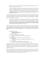
The following is an outline of the minimum amount of information that should be included in such a
justification statement (note that if any of the items is unknown, it is important that this should be
explicitly stated):
(a) State what each species actually does in the ecological context (here or elsewhere) that warrants efforts
to control or eradicate it (e.g., tends to dominate canopy and shade out most other kinds of plants?
prevents regeneration of native species or communities (which ones)? promotes fires and changes fire
disturbance regime? destroys habitat or food resources for wildlife (what species)? causes agricultural
losses (what crops)? is aesthetically objectionable in "natural" areas?); etc.
(b) State where in Hawaii each species is actually creating these general impacts, and where else should
we be concerned that they might do so? (e.g., on what island(s), in what general locations, in what kinds
of habitats? climate zones? broad vegetation types?), etc.
(c) State which specific valued resources each species is negatively affecting at present, and/or others that
might be affected unless control/eradication action is taken (specific private lands, ecological
preserves/National Parks? specific rare "natural" communities? specific critical ecosystems? specific
important watersheds? specific native species? specific endangered species?), etc.
(d) State how something useful can be done about the situation (e.g., of the locations mentioned in (b)
above, in which ones is it "potentially controllable" -- meaning that populations are relatively small and
that biologically effective, culturally and aesthetically acceptable, and cost-effective methods of control are
currently in existence? If not in existence, are they at least being actively researched?), etc.
(e) State who are the major sources of additional local information, and how they may be contacted; also
cite particularly pertinent literature references that are known to provide useful information on the
biology, ecology, climatic preferences, habitat, distribution, and control methods for the species.
Once a reasonably-sized sub-group of "Provisionally High-Priority" species is chosen through some such
preliminary screening process, then the HEAR climatic modeling and risk assessment tools can be used to
compare the potential impacts of each species on environmental resources. Parts 2, 3, and 4 of this
document describe and document in detail the procedures developed by HEAR for this purpose, but they
can be briefly summarized here as follows:
In the first step, each "Provisionally High-Priority" species would be characterized in terms of what is
already known about its general invasive tendencies, conservation impacts, and preferred climatic zones
in other areas worldwide, and the results would be entered on a standard form (see table 1.1 below), using
the categories in tables 1.2 and 1.3.
Each species would also be characterized in terms of what is presently known about its habitat types and
its environmental impacts which are specific to Hawaii, using the categories defined by HEAR in tables
1.4 and 1.5. If desired, a group of experts can be asked to "validate" (i.e., review, correct, and supplement)
this information and provide feedback on the basis of their own knowledge of the alien species and the
environmental conditions in the area(s) of interest.
In the second step, an intensive search of sources in the scientific literature and on the world wide web
would be carried out for these species, but focused primarily on filling in those gaps in our information
base that are relevant to climatic zone preferences, habitats, and impacts. Although not required, it would
be most efficient to record whatever relevant biological and ecological information may turn up during
this literature search, and enter it into the HNIS database for future reference.
In the third step, the ArcView Desktop Geographic Information System (GIS) would be used to construct
digital climatic envelope maps showing the potential distribution in Hawaii of each "Provisionally HighPriority" species, and the relationship of these potential distributions to the known distribution of valued
resources. Specific protocols for this step have been worked out by HEAR (see Parts 2, 3, and 4 of this
report).
In the fourth step, a risk-assessment spreadsheet model would be used to assign an index value to each
"Provisionally High-Priority" alien species, according to its relative potential for causing negative impacts
on environmental assets and resources. Comparison of the index values for all species would provide one
(but not necessarily the only) basis for assigning priorities for control actions over the long term. Specific
protocols for this step have also been worked out by HEAR (see table 1.6).
SECTION 1-5: SOME CAVEATS
Before concluding this overview of HEAR's prototype modeling and risk assessment methods, a few
caveats must be clearly stated.
First, it should be understood that our modeling objective is not to make bullet-proof “predictions” of
future conditions, but rather to enhance our ability to make successively better approximations to reality
under conditions of great uncertainty. This is what Holling (1978) and Walters (1986) have referred to as
the process of "adaptive resource assessment and management". Starfield and Bleloch (1986) have also
emphasized the importance of creating simple but explicitly stated models when dealing with resource
management problems in which there exists:
"...little in the way of supporting data but some understanding of the structure of the problem, [or
in which] ...even the understanding of the problem is tenuous... [Such problems] ...present us two
rather daunting challenges:
1.
From the management point of view, decisions may have to be made despite the
lack of data and understanding. How do we make good, scientific decisions under these
circumstances?
2.
How do we go about improving our understanding and collecting the data we
need?” ...
“Models built [under these limitations] are bound to be speculative. They will never have the
respectability of models built for solving problems in [engineering and physics] because it is
unlikely that they will be sufficiently accurate or that they can ever be tested conclusively. They
should therefore never be used unquestioningly or automatically. The whole process of building
and using these models has to be that much more thoughtful because we do not really understand
the structure of the problem and do not have (and cannot easily get) supporting data.”
“We therefore build models to explore the consequences of what we believe to be true.”...
Second, I have based HEAR’s modeling and risk assessment procedures on the widely-accepted premise
that one of the best predictors of the behavior of alien plants that are invading new areas is knowledge of
their behavior in “similar” environments elsewhere. Therefore, when information obtained from other
geographic areas indicates that a species normally occurs within certain bio-temperature and rainfall
limits, it has been mapped as though it will occur throughout the entire corresponding zone in Hawaii.
But the user needs to be aware that this may or may not reflect the "true" potential distribution of the
species on a particular Hawaiian island (i.e., it could -- probably will -- disperse to and occupy only some
subset of available habitats within that zone on that island).
I have assumed that climatic data obtained from the literature is reliable, and that the HEAR model
correctly extrapolates the given conditions from other geographic areas to Hawaii (detailed support for the
latter assumption is provided in Parts 3 and 4 of this report). Unfortunately, for most environmental
"weeds" it also seems a reasonable assumption that our climatic data set is not necessarily complete.
Moreover, many factors in addition to macro-climate are known to influence plant distribution and
competitive relationships, so the fact that our models may indicate that an alien species can potentially
grow well in a given climatic zone in Hawaii does not mean that it will in fact be able to do so, nor does it
guarantee that if it grows it will become an ecologically dominant or otherwise problematic species.
It is therefore inevitable that someone will find an alien species population growing happily outside its
predicted climatic envelope. If so, I believe that a reasonable response would be to simply add the new
zone to the model; I feel that an unreasonable response would be to immediately declare that the model is
thereby proved to be null and void. I repeat: all models, but especially highly simplified ones like the
HEAR climatic envelope model, require intelligent interaction on the part of the user as well as judicious
interpretation of results. This kind of modeling is meant to be a pragmatic, adaptive process of obtaining
successively better approximations to "reality", not some grand, one-shot-proves-or-disproves-it-all test of
ecological theory.
Third, most actual ecological entities (i.e., populations, communities, and ecosystems) cannot be
represented accurately by the sharp boundary lines that are commonly depicted on small-scale maps. This
should be an obvious point, but it is surprising how often it occurs that knowledgeable people confronted
by a map will forget that real-world boundaries are almost always fuzzy zones of transition, and wind up
making unwarranted assumptions based on what they assume to be clearly demarcated lines. This problem
is worse when one is dealing with such tenuous things as long-term averages of climatic factors which
may actually have been measured at only a few points and then extrapolated to broad areas on the basis of
a very small-scale topographic map.
The potential for errors to arise and propagate through such a data set is great, and the mere fact that this
kind of data may now reside in digital format in a GIS should not lull anyone into thinking that it is
necessarily going to be highly accurate and precise. This is why we have provided metadata files along
with our climatic and vegetation zone maps, as well as the present document discussing underlying theory
and methods -- this information should be read carefully, and the maps interpreted accordingly!
Fourth, although spatial scale is repeatedly discussed throughout this report, little attention is given to
considerations of temporal scale. This is due to the fact that I have deliberately restricted myself to a
methodology that stresses geographic distribution while requiring a minimum amount of biological and
ecological information collected over "a suitably long period of time". Nevertheless, the temporal factor is
important when dealing with risk assessment, since it begins to address the issue of successional
trajectories in the vegetation.
Many (most?) "weedy" species are primarily adapted to take advantage of conditions in areas that have
been recently disturbed - whether by humans, alien animals, natural canopy dieback events, hurricanes, or
other factors. After colonizing an area, populations of weeds may often achieve large numbers within a
disturbance patch (and perhaps even attain ecological dominance there, which is not necessarily the same
thing). However, this short-term behavior says little about whether such species will be able to maintain
their high population numbers in that area, or whether they will be able to spread into adjacent
undisturbed areas.
Under some conditions in some systems, invading plant species may be virtually eliminated from an area
(or at least suffer greatly reduced numbers) simply due to normal biological and ecological processes
during succession. If this were to occur within a time period significantly shorter than the typical local
disturbance return interval, then it is possible that the alien species may not actually pose a severe threat
to the integrity of that ecological system, early appearances notwithstanding.
The point is that, in addition to inquiring about whether an alien species can or cannot invade a certain
area, decision-makers also need to assess the return intervals and other characteristics of the regional and
local disturbance regimes, the possibility that a given alien species either will or will not be eliminated (or
significantly reduced) during the course of succession before the next disturbance, and the degree to which
the valued resources in the area may be affected by that species both in the short term and in the long
term. This goes beyond the capabilities of the simple risk assessment system presented here.
SECTION 1-6. FUTURE WORK: INCORPORATING BIOLOGICAL AND ECOLOGICAL
FACTORS INTO THE ASSESSMENT
I believe that it should be possible to significantly improve on the predictive capability of the prototype
HEAR climatic envelope models IF some method were available for factoring in the biological and
ecological interactions which strongly influence the establishment, survival, reproduction, and dispersal of
each alien species in a particular ecological system.
For example, Tucker and Richardson (1995) have created a prototype computerized "expert system" for
the Fynbos Biome in South Africa, which assigns each alien plant species to either a "High-Risk" or a
"Low-Risk" category. This goes the extra step beyond the current HEAR system by taking into account
critical biological and ecological characteristics of the species in relation to constraining or facilitating
factors of the environment that are found within a given macro-climatic zone.
The biological and ecological characteristics of alien plants that are considered in Tucker and
Richardson's (1995) expert system fall into six main categories: Preferences for Broad-scale
Environmental Factors and Disturbance Regime (e.g., macro-climate, soil nutrient level, successional
stage); Population Characteristics (e.g., whether thicket-forming or "weedy") and Habitat Specialization
(yes/no; if yes, whether biologically determined or not); Dispersal Mechanisms (e.g., principal vector in
home environment; is this vector or some equivalent present/absent in this biome); Seed Production (e.g.,
high/low; and is this genetically or biotically determined); Seed Predation (e.g., is an effective predator
present/absent in this biome); and Special Life History Adaptations (e.g., fire resistance, seed bank
longevity).
Although the task in Hawaii may perhaps be more difficult than in the Fynbos biome (a system strongly
constrained by recurrent drought and fires), the development of risk assessment models incorporating
biological and ecological constraints does not seem totally out of the realm of possibility -- if efforts are
focused on the "potentially high-risk" alien species in certain “critical” ecological systems. One obvious
candidate for a critical system would seem to be Hawaii's Warm Temperate Wet climate zone where much
of the state's remaining terrestrial biodiversity is found (and where the zonal "montane rainforest"
vegetation also appears to be strongly constrained by physical factors; cf. Kitayama and Mueller-Dombois
1992, 1994a, 1994b).
Unfortunately, for many of the alien species classified as “environmental” rather than “agricultural”
weeds, good information regarding their biological and ecological characteristics tends to be rather scarce
in the literature. Even if published information is already available from other areas in the world, some
amount of field research will still be required to verify if and how these characteristics are expressed in
particular Hawaiian environmental systems. One important effect of developing an expert system model
would be to focus field research on closing the gaps in our current knowledge. Over the long term, the
effort required to carry out this more detailed level of data collection and modeling would be repaid in
terms of a greater understanding of the interactions among alien species, indigenous species, and
environment in the selected system(s). This should lead to better decision-making by scientists and land
managers about the benefits versus the costs of control and eradication efforts.
But (once again) perhaps the largest pay-off of creating better models may be in terms of their impact on
non-specialist decision-makers in local, state, and federal governments -- these are the people who will
need more than hand-waving arguments and “horror stories” to convince them to support control or
eradication actions against a alien species (Richardson, 1997).
REFERENCES FOR PART 1:
Allen, T. and Hoekstra, T. 1992. Toward a unified ecology. Columbia University Press, NY.
Clunie, N. M. W. 1995. A strategy for management of plant pests in Auckland Conservancy. Clunie and
Associates, Environmental Consultants for Auckland Conservancy, Department of Conservation,
Auckland, New Zealand.
Cronk, Q. and Fuller, J. 1995. Plant Invaders. Chapman and Hall, London.
Holling, C. (ed.). 1978. Adaptive Environmental Assessment and Management. John Wiley & Sons, New
York.
Kitayama, K. and Mueller-Dombois, D. 1992. Vegetation of the wet windward slope of Haleakala, Maui,
Hawaii. Pacific Science 46(2): 197-220.
Kitayama, K. and Mueller-Dombois, D. 1994a. An altitudinal transect of the windward vegetation on
Haleakala, a Hawaiian island mountain: (1) climate and soils. Phytocoenologia 24: 111-133.
Kitayama, K. and Mueller-Dombois, D. 1994b. An altitudinal transect of the windward vegetation on
Haleakala, a Hawaiian island mountain: (2) vegetation zonation. Phytocoenologia 24: 135-154.
Richardson, D. 1997. (One of the developers of the Fynbos model, pers. com. to R. Teytaud).
Starfield, A. and Bleloch, A. 1986. Building models for conservation and wildlife management.
MacMillan Publ. Co., N.Y.
Tucker, K. and Richardson, D. 1995. An expert system for screening potentially invasive alien plants in
South African Fynbos. Jour. Environ. Manage. 44: 309-338.
Walters, C. 1986. Adaptive Management of Renewable Resources. McGraw-Hill, New York.
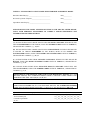
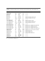
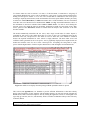
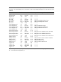
TABLE 1.1: EXAMPLE DATA & RAW SCORE SHEET FOR RISK ASSESSMENT MODEL
Data Sheet Data Entry by:_____________________________
Date___________
Reviewed by (Name of Expert):_________________________
Date___________
Spreadsheet Data Entry by:____________________________
Date___________
PLEASE REVIEW THE CODES ASSIGNED BY HEAR TO THE SPECIES LISTED BELOW,
USING YOUR PERSONAL KNOWLEDGE TO CORRECT AND/OR SUPPLEMENT THE
INFORMATION PROVIDED BY HEAR.
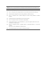
TO THE RIGHT OF THE SPECIES NAME, UNDER "CATEGORY CODES":
(A) PLEASE ENTER EVERY CRONK AND FULLER "INVASIVE CATEGORY" WHICH FITS THE
SPECIES ELSEWHERE IN THE WORLD, USING THE NUMBER CODES GIVEN IN TABLE 1.2,
SEPARATED BY COMMAS; e.g., 1.5, 4.5
(B) PLEASE ENTER EVERY CRONK AND FULLER "CLIMATE ZONE" IN WHICH THE SPECIES
IS KNOWN TO THRIVE ELSEWHERE IN THE WORLD, BOTH IN ITS NATIVE AND
NATURALIZED RANGES, USING THE LOWER CASE LETTER CODES GIVEN IN TABLE 1.3,
SEPARATED BY COMMAS; e.g., m, n, o
(C) PLEASE ENTER EVERY HEAR "INVASIVE CATEGORY" WHICH FITS THE SPECIES IN
HAWAII, USING THE ROMAN NUMERAL CODES GIVEN IN TABLE 1.4, SEPARATED BY
COMMAS; e.g., I, IV
(D) PLEASE ENTER EVERY HEAR "NEGATIVE IMPACT CATEGORY" WHICH FITS THE
SPECIES IN HAWAII, USING THE NUMBER CODES GIVEN IN TABLE 1.5, SEPARATED BY
COMMAS; e.g., 2, 4
PLEASE REPEAT THIS PROCESS FOR EACH OF THE REMAINING SPECIES (E.G., FOR
THE FIRST SPECIES, THE COMPLETED ENTRY UNDER "CATEGORY CODES" MIGHT LOOK
SOMETHING LIKE THIS: 1.5, 4.5, m, n, o, I, IV, 2, 4
SCORING: HEAR PROJECT STAFF WILL CALCULATE THE RAW SCORES, FOLLOWING THE
INSTRUCTIONS IN TABLE 1.6 (E.G., FOR THE FIRST SPECIES, THE COMPLETED ENTRIES
UNDER "RAW SCORES" MIGHT LOOK LIKE: (1) 4.5 (2) 3 (3) 2 (4) 4 (5) 4 (6) 5 (7) 168 (8) 60
Species Name
Acacia mearnsii
Acacia melanoxylon
Casuarina equisetifolia
etc, etc.
Category Codes (from Tables 1.2 to 1.5)
Raw Scores (from Table 1.6)
(1)__(2)__(3)__(4)__(5)__(6)__(7)__(8)__
(1)__(2)__(3)__(4)__(5)__(6)__(7)__(8)__
(1)__(2)__(3)__(4)__(5)__(6)__(7)__(8)__
TABLE 1.2: Invasive Categories Elsewhere for Alien Species Present in Hawaii (after Cronk and Fuller 1995)
Code
1.0
Invasive Categories Elsewhere
Minor weed of highly disturbed or cultivated land (man-made artificial landscapes)
1.5
Serious or widespread weeds of highly disturbed or cultivated land (man-made artificial landscapes)
2.0
Weeds of pastures managed for livestock, forestry plantations or artificial waterways
2.5
Serious or widespread weeds of pastures managed for livestock, forestry plantations or artificial
waterways
3.0
Invading semi-natural or natural habitats (some conservation interest)
3.5
Serious or widespread invaders of semi-natural or natural habitats
4.0
Invading important natural or semi-natural habitats (i.e., species-rich vegetation, nature reserves, areas
containing rare or endemic species)
4.5
Serious or widespread invaders of important natural or semi-natural habitats (i.e., species-rich
vegetation,
nature reserves, areas containing rare or endemic species)
5.0
Invasion threatening other species of plants or animals with extinction
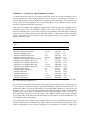
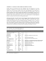
TABLE 1.3: Worldwide Climate Zones for Alien Species Present in Hawaii (after Cronk and Fuller 1995)
Climate Zone
PET
PPT (mm)
BT (C) Equivalent Holdridge Life Zone(s) in Hawaii
Subpolar dry
1-2
<125
1.5-3
----------Subpolar moist
0.5-1
125-250
1.5-3
----------Subpolar wet
<0.5
>250
1.5-3
----------Boreal arid
>2
<125
3-6
----------Boreal dry
1-2
125-250
3-6
----------Boreal moist
0.5-1
250-500
3-6
Subtropical Subalpine Moist Forest
Boreal wet
0.25-.5 500-1000
3-6
Subtropical Subalpine Wet Forest
Boreal wet
<0.25
>1000
3-6
----------Cool Temperate arid
>2
<250
6-12
----------Cool Temperate dry
1-2
250-500
6-12
Subtropical Montane Steppe
Cool Temperate moist
0.5-1
500-1000
6-12
Subtropical Montane Moist Forest
Cool Temperate wet
0.25-.5 1000-2000 6-12
Subtropical Montane Wet Forest
Cool Temperate wet
<0.25
>2000
6-12
----------Warm Temperate arid
>4
<250
12-18
----------Warm Temperate arid
2-4
250-500
12-18
Subtropical Lower Montane Thorn Woodland
Warm Temperate dry
1-2
500-1000
12-18
Subtropical Lower Montane Dry Forest
Warm Temperate moist
0.5-1
1000-2000 12-18
Subtropical Lower Montane Moist Forest
Warm Temperate wet
<0.5
>2000
12-18
Subtropical Lower Montane Wet & Rain Forest
Subtropical arid
>8
<125
18-24
----------Subtropical arid
2-8
125-500
18-24
Subtropical Desert Scrub & Thorn Woodland
Subtropical dry
1-2
500-1000
18-24
Subtropical Dry Forest
Subtropical moist
0.5-1
1000-2000 18-24
Subtropical Moist Forest
Subtropical wet
<0.5
>2000
18-24
Subtropical Wet & Rain Forest
Tropical arid
>2
<1000
>24
----------Tropical dry
1-2
1000-2000 >24
----------Tropical moist
0.5-1
2000-4000 >24
----------Tropical wet
<0.5
>4000
>24
----------*Note: PET = potential evapotranspiration ratio (dimensionless); PPT = mean annual precipitation (mm);
BT = mean annual bio-temperature (C)
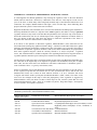
TABLE 1.4: HEAR Invasive Categories for Alien Species Present in Hawaii
Code
I
Invasive Categories
Invading "disturbed" land or "early successional" land other than agricultural landscapes in Hawaii
(i.e., whether disturbed by "natural" causes or "human-mediated" causes)
II
Invading cultivated crops, or man-made pastures managed for livestock in Hawaii
III
Invading forestry plantations in Hawaii
IV
Invading "relatively undisturbed", non-cultivated, "middle-to-late successional"," semi-natural" or
"natural" open habitats in Hawaii (e.g., bogs, dunes, grassland, shrubland, savanna, etc.)
V
Invading "relatively undisturbed", non-cultivated, "middle-to-late successional", "semi-natural" or
"natural" open woodland habitats in Hawaii
VI
Invading "relatively undisturbed", non-cultivated, "middle-to-late successional", "semi-natural" or
"natural" closed-forest habitats in Hawaii
TABLE 1.5: HEAR Negative Impact Categories for Invasive Alien Species Present in Hawaii
Code
1
Negative Impacts Known (or Strongly Suspected) to be Caused by This Species in Hawaii
Invasion of this species is known or suspected to cause economic losses on "developed " agricultural
lands;
housing, commercial, or industrial areas; developed parklands or recreational areas; or any other lands
whose primary values lie in their socio-economic/cultural rather than ecological features and assets)
2
Invasion of this species is known or suspected to cause significant alterations of the natural fire regime of
ecosystems and/or landscapes; and/or invasion of this species is presently known to cause significant
alterations of energy flows, materials and nutrients cycling, moisture relationships, and/or other critical
processes of ecosystems; and/or invasion of this species is presently known to cause significant alterations
of the soil chemistry or the soil erosion characteristics of ecosystems and/or landscapes
3
Invasion of this species is known or suspected to cause replacement of natural and/or semi-natural
systems of high diversity and/or ecological value with systems of significantly lower diversity and/or
ecological value, when considered under community, ecosystem, landscape, and/or macro-climatic zone
(vegetation zone or biome) criteria; and/or invasion of this species is presently known to pose some
significant direct threat to the well-being of native faunal or floral communities in general, or of species
with some special conservation (e.g., rare, threatened, endangered, etc.) or ecological status
4
Invasion of this species is known or suspected to pose some significant direct threat of local, regional,
insular, statewide, or global extinction(s) of native species; and/or of species having some special
conservation (e.g., rare, threatened, endangered, etc.) or ecological status
TABLE 1.6: Scoring System for Use with the HEAR Risk Assessment Model
Score
Score #1
Rules for Computing Raw Scores
"HIGHEST Cronk and Fuller Invasive Category (in terms of the number codes in table 1.2)
presently known for this species ELSEWHERE IN THE WORLD", based on information obtained
from Cronk and Fuller (1995) and/or other literature and/or expert opinion (leave blank only if
information is unavailable)
Score #2
"TOTAL NUMBER of different types of Cronk and Fuller Climate Zones (in terms of table 1.3)
presently known to be occupied by this species ELSEWHERE IN THE WORLD", based on
information obtained from Cronk and Fuller (1995) and/or other literature and/or expert opinion
(leave blank only if information is unavailable)
Score #3
"HIGHEST HEAR Invasive Category (in terms of the number codes in table 1.4) presently known
for this species on the main Hawaiian islands", based on information from the literature and/or
expert opinion (leave blank only if information is unavailable)
Score #4
"HIGHEST HEAR Negative Impact Category (in terms of the number codes in table 1.5) presently
known for this species on the main Hawaiian islands", based on information from the literature
and/or expert opinion (leave blank only if information is unavailable)
Score #5
"TOTAL NUMBER of different types of HEAR Climate Zones within the climate envelope of the
species in Hawaii, and presently/potentially invaded by this species on the main Hawaiian islands";
calculated using information from the HEAR climate envelope GIS model (leave blank only if
information is unavailable)
Score #6
"TOTAL LAND AREA (square miles) of HEAR Climate Zones within the climate envelope of the
species in Hawaii, and potentially invadable by this species on the main Hawaiian islands";
calculated using information from the HEAR climate envelope GIS model (leave blank only if
information is unavailable)
Score #7
"TOTAL LAND AREA (square miles) of existing Natural/Semi-Natural Physiognomic Vegetation
Types (i.e., Ecoregional Sub-Units) potentially invadable if this species were to attain its potential
distribution on the main Hawaiian islands", calculated by intersecting the HEAR climate envelope
GIS model with TNCH's digital map of Ecoregional Sub-Units - enter 0 if no such area is believed
to be threatened (leave blank only if information is unavailable)
Score #8
"TOTAL LAND AREA (square miles) of Managed Areas potentially invadable if this species were
to attain its potential distribution on main Hawaiian islands", calculated by intersecting the HEAR
climate envelope GIS model with TNCH's digital map of Managed Areas - enter 0 if no such area is
believed to be threatened (leave blank only if information is unavailable)
PROTOTYPE TOOLS FOR RISK ASSESSMENT OF ALIEN PLANT INVASIONS IN HAWAII:
A REPORT OF THE HAWAII ECOSYSTEMS AT RISK (HEAR) PROJECT
PART 2a: USER'S GUIDES TO THE MODELING TOOLS
Robert Teytaud, Project Leader
Hawaii Ecosystems At Risk (HEAR) Project
Revised 6/22/98
PROTOTYPE TOOLS FOR RISK ASSESSMENT OF ALIEN PLANT INVASIONS IN HAWAII:
A REPORT OF THE HAWAII ECOSYSTEMS AT RISK (HEAR) PROJECT
PART 2a: USER'S GUIDES TO THE MODELING TOOLS
Robert Teytaud, Project Leader
Hawaii Ecosystems At Risk (HEAR) Project
Revised 6/22/98
MAJOR SECTION HEADINGS IN PART 2a:
SECTION 2a-1. USER'S GUIDE #1: INTRODUCTION TO THE GIS MAPS
SECTION 2a-2. USER'S GUIDE #2: CLIMATIC ENVELOPE MODELS
SECTION 2a-3. USER'S GUIDE #3: RISK ASSESSMENT SPREADSHEET MODELS
REFERENCES FOR PART 2a
Note: The User's Guides in this document provide the basic information needed to access, manipulate, and
correctly interpret HEAR’s prototype modeling tools. However, some familiarity with digital mapping
procedures and windows-based personal computer applications in general -- and with the ArcView 3 and
Excel 7 programs in particular -- is assumed on the part of the user. ArcView and ArcInfo are Geographic
Information System applications by ESRI, Inc.; Excel 7 is a spreadsheet application by Microsoft, Inc.
SECTION 2a-1. USER'S GUIDE #1:
INTRODUCTION TO THE GIS MAPS
Throughout this document, I will be making frequent reference to "GIS maps". I use this loose and somewhat inaccurate term to avoid
introducing technical GIS terminology that may confuse some readers. For those who already know the jargon, I simply point out that what
I call a GIS map corresponds to a "View" in ArcView terms. Each GIS map (or view) contains one or more "Themes" (analogous to
different “map layers" that can be turned on or off). Themes actually consist of individual computer files that may be stored in any of a
number of different formats (e.g., ArcView shapefiles, GPS coordinate files, ArcInfo coverages, remote-sensing images, AutoCAD drawing
files, graphics files, etc.); ArcView is able to display any of these file types as a component of a GIS map.
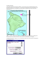
A set of thirteen GIS maps, together with their tabular data files and ancillary files of various types, are
stored on the HEAR distribution disk within a single master directory named "Environment". The main
ArcView project file that controls all of the others is named "Environ.apr". Taken together, all of these
files comprise the "HEAR Climatic Envelope Project", a prototype system designed to model the potential
geographic distribution of alien plant species in Hawaii.
The digital base maps used for the Climatic Envelope Project are a set of standard ArcInfo coverages of
the main Hawaiian Islands (UTM coordinates, Zone 4, Old Hawaiian Datum), which were obtained by
HEAR in 1996 from the now-defunct Hawaii Office of State Planning (OSP). To the best of our
knowledge these OSP coverages were derived from standard USGS digital source files.
I used a small (12" x 12") digitizing tablet, accurate to 0.001 inch, to capture the generalized island-scale
distribution of vegetation and major climatic factors (i.e., rainfall and temperature) from copies of maps
which appear in various publications, and I used ArcView 3 to register the digitized maps to the OSP
digital map base. I recorded information (metadata) on source materials, etc. for each digitized map in the
“Comments” area of the Theme Properties dialog box. All digital maps were saved in the ArcView
shapefile format, which also enables them to be used in other, more sophisticated, Geographic Information
Systems such as ArcInfo.
IMPORTANT NOTICE: The ArcView 3 program expects to find the main Climatic Envelope Project file
(named Environ.apr) and all associated files in a directory named "Environment", located in the same
"path" where they were originally stored on the HEAR computer; i.e., C:\Arcview\Avdata2_Environ\
Environment\
BEFORE OPENING THIS PROJECT FOR THE FIRST TIME, you should first create the following
"path" on the C DRIVE of your computer: C:\Arcview\Avdata2_Environ; then copy the ENTIRE
"Environment" directory off the distribution disk (e.g., a Syquest 135 MB or Zip cartridge) to the
Avdata2_Environ directory that you just created.
PLEASE run the Climatic Envelope Project only AFTER transferring the Environment directory to the C
DRIVE of your computer, and keep your original distribution disk as a backup. DO NOT open the project
file from the distribution disk! Failure to follow the above procedure will not destroy any files, but it
WILL result in the loss of the essential links among the project files. The only cure for this is an extremely
tedious, hours-long session in which ArcView will ask you to specify the location of each and every file.
Description of the HEAR GIS Maps
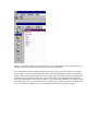
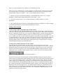
To begin working with the GIS maps, start up the ArcView program and navigate to the Environment
directory on your C drive, then double-click on the Environ.apr file. When the Environ.apr window comes
up, click on the "Views" icon at the left side to see a listing. Thirteen view names starting with the letters
"A" through "M" will appear; simply double-click on the name corresponding to the GIS map that you
wish to display (all of the main Hawaiian islands are shown on each of the maps, except for maps I, J, and
K which cover the "Big Island" only).
Each GIS map generally has associated with it a tabular database containing information (e.g., area,
polygon type, island, etc.) for each individual polygon. The databases can be accessed in ArcView in the
normal manner (i.e., from the menus or by clicking on the appropriate icon in the toolbars).
GIS maps A to C are the source material for all the HEAR maps that are based on the Holdridge Life Zone
model or its modifications (i.e., maps D, E, F, and M). GIS maps G to L depict various other climate and
vegetation zone schemes which are commonly encountered in journal articles, in the worldwide botanical
and bio-geographic literature, and in the recent review volume "Vegetation of the Tropical Pacific
Islands" (Mueller-Dombois and Fosberg 1998) -- these maps provide a means of roughly translating
climatic information given in terms of these other schemes into the Holdridge-based climate zones in
Hawaii. GIS map M displays the prototype climatic envelope models created for each Hawaiian island
using the HEAR climate zone system that will be described below.
The locations of the transect lines sampled in several important studies (e.g., Kitayama and MuellerDombois 1992, 1994a, 1994b; Mueller-Dombois et al. 1981) of macro-climatic factors, soils, plant
communities, and other biota in major ecological systems on the Big Island and Maui have been added to
some of the GIS maps. This was done so that the ground-based data reported in these papers, and the
photographs illustrating different vegetation types, can be easily correlated with HEAR's GIS maps.
Approximate locations for the winter season frequent-frost line and the daily frost line -- important
potential limiting factors for plant growth -- have been added to most of the GIS maps, along with
topographic contours (1,000-ft intervals) and major roads.
Some maps also contain themes displaying the outlines of polygons taken from certain other maps in the
series; these outline themes may be toggled on or off so as to facilitate comparisons between the maps.
Brief descriptions of each of the HEAR GIS maps and their sources are as follows:
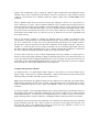
A. Mean Annual Air Temperature, after the Nullet and Sanderson (1993) map of mean annual
air temperature isotherms (degrees C.) for the main Hawaiian islands.
B. Mean Annual Rainfall, after the Giambelluca et al. (1986) map of mean annual rainfall
isohyets (mm) for the main Hawaiian islands, adapted by grouping the isohyets into appropriate
classes corresponding to the index values on the standard Holdridge life zone diagram (Holdridge
1967).
C. Holdridge Altitudinal Belts, derived by grouping the mean annual temperature isotherms
from GIS Map (A) into appropriate bio-temperature classes according to Holdridge (1967); this
aggregation process required interpolation of some isotherms from data provided on the original
maps.
D. Holdridge Life Zones, derived by intersecting the mean annual rainfall isohyets shown on
GIS Map (B) with the Holdridge altitudinal belts shown on GIS Map (C).
E. Cronk and Fuller Climate Zones, derived by a process of aggregating the Holdridge life
zones shown on GIS Map (D) into the appropriate larger units as given by Cronk and Fuller
(1995) in their book on invasive plants.
F. Cramer and Leemans Climate Zones, derived by a process of aggregating the Holdridge life
zones shown on GIS Map (D) into appropriate larger units as given by Cramer and Leemans
(1993) in their paper on the major worldwide vegetation types and climate classification systems.
G. Potential Vegetation Zones/Characteristic Native and Alien Species, after the vegetation
zone map of Ripperton and Hosaka (1942); vegetation zone names consist of the alphanumeric
codes from the original map, supplemented by the existing dominance-type designations given by
Lamoureaux (1986) in the Atlas of Hawaii.
H. Potential Vegetation Zones/Physiognomic-Structural Types, after the vegetation zone map
of Ripperton and Hosaka (1942); vegetation zone names consist of the alphanumeric codes from
the original map, supplemented by the physiognomic-structural type designations of MuellerDombois (1982). Note that the vegetation zone boundaries are identical to GIS Map (G) -EXCEPT that a modified boundary consistent with the findings of Kitayama and MuellerDombois (1994a) is shown between zones D1 (Lowland Rainforest) and D2 (Montane
Rainforest).
I. Koppen Climate Zones (Big Island), after Giambelluca and Sanderson (1993).
J. Thornthwaite Climate Zones (Big Island), after Giambelluca and Sanderson (1993).
K. Thornthwaite Moisture Regimes (Big Island), after Giambelluca and Sanderson (1993).
L. Knapp Climatic Vegetation Zones, after Mueller-Dombois and Fosberg (1998), who state
that the zones are based on the distribution of certain (unspecified) "indicator species" as given
by Knapp (1965) slightly modified according to the Walter-type climate diagrams shown in
Mueller-Dombois et al. (1981).
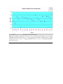
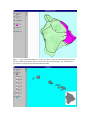
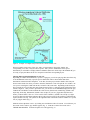
M. Demonstration Climatic Envelope Models: Potential Distributions of Alien Plants Based
on HEAR Climate Zones, derived by "querying" the HEAR climate zone map to select areas on
each main island which match climatic preference information obtained from the literature. Each
climatic envelope model appears as a separate theme in the view's table of contents (in cases of
conflicting information, there may be more than one model for a species). All sources on which a
given climatic envelope model is based are documented in the "Comments" area of the Theme
Properties dialog box for that map.
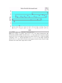
The HEAR climate zones shown in GIS Map M were created by aggregating seven of the Cronk and
Fuller climate zones into three larger units. These three composite units (which occur only on the Big
Island and Maui) include the entire Boreal altitudinal belt, the entire Cool Temperate altitudinal belt, and
the Arid and Dry portions of the Warm Temperate altitudinal belt. These zones were combined to achieve
a closer fit to the boundaries of actual and potential physiognomic vegetation types ("ecoregional subunits") that have been mapped by The Nature Conservancy of Hawaii (see further discussion in Section 22 below, and in Section 3-6 in Part 3 of this document).
In the new aggregated HEAR system there are a total of nine climate zones in Hawaii, compared to ten in
the Cramer and Leemans system, thirteen in the Cronk and Fuller system, and sixteen in the original
Holdridge system. The names of the HEAR zones and the Cronk and Fuller zones are given below;
followed in brackets by the name of the TNCH ecoregional sub-unit which occupies the largest part of
each HEAR zone.
(1). HEAR Subtropical Arid Climate Zone < 500 mm mean ann. rainfall; same as Cronk and
Fuller's Subtropical Arid Climate Zone [TNCH Lowland Dry Shrubland/Grassland]
(2). HEAR Subtropical Dry Climate Zone 500-1000 mm mean ann. rainfall; same as Cronk and
Fuller's Subtropical Dry Climate Zone [TNCH Lowland Dry Forest/Shrubland]
(3). HEAR Subtropical Moist Climate Zone 1000-2000 mm mean ann. rainfall; same as Cronk
and Fuller's Subtropical Moist Climate Zone [TNCH Lowland Mesic Forest/Shrubland]
(4). HEAR Subtropical Wet Climate Zone > 2000 mm mean ann. rainfall; same as Cronk and
Fuller's Subtropical Wet Climate Zone [TNCH Lowland Wet Forest/Shrubland]
(5). HEAR Warm Temperate Arid/Dry Climate Zone 250-1000 mm mean ann. rainfall; includes
Cronk and Fuller's Warm Temperate Arid and Warm Temperate Dry Climate Zones [TNCH
Montane Dry Forest/Shrubland]
(6). HEAR Warm Temperate Moist Climate Zone 1000-2000 mm mean ann. rainfall; same as
Cronk and Fuller's Warm Temperate Moist Climate Zone [TNCH Montane Mesic Forest/
Shrubland]
(7). HEAR Warm Temperate Wet Climate Zone > 2000 mm mean ann. rainfall; same as Cronk
and Fuller's Warm Temperate Wet Climate Zone [TNCH Montane Wet Forest/Shrubland]
(8). HEAR Cool Temperate Dry/Moist/Wet Climate Zone 250-2000 mm mean ann. rainfall;
includes Cronk and Fuller's Cool Temperate Dry, Cool Temperate Moist, and Cool Temperate
Wet Climate Zones [TNCH Subalpine DryForest/Shrubland/Grassland]
(9). HEAR Boreal Moist/Wet Climate Zone 250-1000 mm mean ann. rainfall; includes Cronk
and Fuller's Boreal Moist and Boreal Wet Climate Zones [TNCH Alpine, undifferentiated]
SECTION 2a-2: USER'S GUIDE #2:
CLIMATIC ENVELOPE MODELS
The particular set of climatic envelope models included as separate themes in the HEAR Climate Zone
map corresponds to all alien plant species identified as "potentially controllable" in the HEAR Island
Matrix for which climatic zone data was available in Cronk and Fuller (1995). It is worth emphasizing
that the ONLY worldwide data used to construct these demonstration models comes straight out of this
single book; while it is probably as trustworthy a source as any, there is no guarantee that this information
is complete. In many instances, there may be NO local data whatsoever represented in a given climate
envelope model, unless data from Hawaii just happened to be included in Cronk and Fuller.
In light of this data limitation, the demonstration HEAR climate envelope models are to be interpreted as
follows: IF the climate zones which were reported in Cronk and Fuller are truly representative of the
limits of distribution of a given species ELSEWHERE in the world, and IF any additional zones where the
species is currently KNOWN to occur locally are added to the models, THEN the models should represent
a good first approximation to the ENTIRE POTENTIAL climatic distribution of the species in Hawaii.
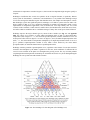
HEAR's climate zones and climatic envelope modeling methods are based on the well-known system of
worldwide bio-climatic zones originally developed by Holdridge (1967) and later modified by Cronk and
Fuller (1995), Cramer and Leemans (1993), and others. Although various other researchers (e.g.,
Pheloung 1995, 1996) have developed climatic envelope procedures to predict distributions of alien
species elsewhere in the world, as far as I am aware the method discussed here is the only one based on
the Holdridge life zone classification system or its derivatives.
The advantages of using a Holdridge-type life zone approach are: first, that it provides a standardized
terminology and methodology for comparing climates and climatically-controlled ecological systems in
Hawaii with those occurring elsewhere in the world; second, that the quantitatively defined and mapped
climatic zones form a hierarchical system which can be aggregated or disaggregated into units of larger or
smaller sizes as necessary to fit the requirements of the analysis; and third, that climatic envelope
projections can be made by utilizing only the most widely available kind of climatic data, i.e., mean
annual rainfall, mean annual temperature, and summaries of the monthly means and extremes for these
variables.
In the absence of consensus on biological/ecological criteria for predicting "degree of invasiveness", and
in order to generate a worst-case scenario for a given alien species, the HEAR method projects the
total area (i.e., the climatic envelope) which may be susceptible to invasion by that species. That is, I
assume (as a first approximation) that the sole natural constraint on the spread of an alien species on a
given island is the pattern of prevailing macro-climates in which it is able to thrive, and that no artificial
control is applied to keep it in check.
I intentionally ignore all other biological/ecological interactions that might alter the climatic and biotic
potential of a species, or affect its ecological potential to attain dominance over other competing species in
the same habitats. Under these simplifying assumptions we are able to generate potential distribution
maps which serve as input to a risk assessment model; the latter then computes a set of index scores which
allows us to more-or-less "objectively" compare different alien species in terms of their "relative potential
for environmental impact".
The assumptions underlying the climatic envelope method can be cast in the form of a very simple but
potentially falsifiable null hypothesis (as usual, rejection of the null hypothesis is the expected outcome).
Note that I am not suggesting that statistical testing of the null hypothesis would be practical, or
necessary, for the present purposes of the HEAR project. The point of framing a null hypothesis is merely
to be as clear as possible about what a climatic envelope model actually means, in the interest of
forestalling any unwarranted assumptions on the part of the user.
NULL HYPOTHESIS: "If tested by field surveys carried out on a given Hawaiian island for 'a suitably
long period of time', there will be no significant difference (say at the 90% level) between the probability
of occurrence of an alien plant species within its climatic envelope on that island, and the probability of
occurrence of this species outside its climatic envelope." REJECTION of this hypothesis would imply that
the climatic envelope IS a successful predictor of the geographic area of a particular island within which
that alien plant species occurs.
Generating a New Climatic Envelope Model
Once the necessary information on geographic distribution and climatic preferences has been collected
from the literature, local experts, and other sources, it is a simple matter to create a climatic envelope
model for a given species (it takes longer to describe the process step-by-step than it takes to actually do
it).
Start by opening GIS map M (Demonstration Climatic Envelope Models: Potential Distributions of Alien
Plants Based on HEAR Climate Zones), and create a new theme that shows the currently known
distribution for the species in Hawaii. If you are fortunate, a map of the current distribution may already
be available from the HEAR project (or other sources) in the form of digitized map polygons or GPS
points, in which case you can just add it as a theme to GIS map M. If a digital map does not already exist
and you have no information that will allow you to create one yourself, then move on to the next step -you can always add current distribution data as it becomes available.
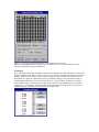
Next, make a copy of the "HEAR Climate Zones" theme in GIS map M by first selecting it and then
choosing "Copy Theme" under the Edit menu; an identical copy of this theme will appear at the top of the
view's table of contents. Select the copied theme in the table of contents by clicking on it, then doubleclick on its name so as to bring up the Legend Editor.
The box labeled "Legend Type" in the Legend Editor will say "Unique Values". Click on the downwardpointing arrow to the right of the box to pull down the list of legend types and choose "Single Symbol"; all
polygons in the theme will now be displayed in some uniform color randomly selected by the program.
Double-click on the "Symbol" rectangle to bring up the Fill Palette; scroll down and choose some bold
pattern (thick horizontal bars, say, like those in the HEAR demonstration model).
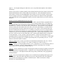
Now click the Color Palette button at the top of the Fill Palette, and when the Color Palette appears select
some bright color for the Foreground color, then select none for the Background color, and none for the
Outline color. Click the "Apply" button in the lower right-hand corner of the Legend Editor, then close
both the Legend Editor and the Color Palette.
Next, choose "Theme Properties" from the Theme menu. Make sure that the icon labeled "Definition" is
highlighted in the list at the left of the "Theme Properties" dialog box, then rename the copied theme as
appropriate (e.g., enter "Clidemia hirta Potential Distrib." in the box at the top labeled "Theme Name").
The next step is very important: in the box labeled "Comments" type in a brief note documenting the
sources of the information you are using to create the climatic envelope model (see the various examples
in the HEAR demonstration models).
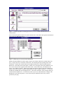
Now you are ready to define the subset of map polygons comprising the new climatic envelope model.
Click on the button in the "Theme Properties" dialog box that has a picture of a hammer on it (to the left
of the Definition box) and the "Query Builder" dialog box will come up. At the left-hand side, scroll down
through the list labeled "Fields" until you find a field labeled "HEAR Climate Zone" and double-click on
it; the name of this field will be added to the Definition box. Click the [=] button, then scroll down
through the list labeled "Values" at the right-hand side until you find a field labeled with one of the
climate zones from which the species has been reported; double-click it to add this value to the definition.
The species for which you are creating the model will often occur in more than one climate zone. To add
additional zone names to the definition, click on the [or] button and then repeat the above procedure of
clicking the "HEAR Climate Zone" field, the "equals" button, and the appropriate "Values" field. Click
the [or] button again and repeat this procedure until you have included all the zones from which the
species is known elsewhere in the world, as well as in Hawaii. Then click the OK button at the bottom.
One more thing remains to be done: calculating and converting the areas of the polygons in the climatic
envelope model. Display the theme's table by clicking on the "Table" button in ArcView's tool bar. Then
choose "Start Editing" under the Table menu and highlight the "Area" field, then click the "Field
Calculator" button. In the dialog box that comes up, you will build an expression telling ArcView what
values to put in the Area field.
In the "Fields" scrolling list, double-click on the "Shape" field and the program will add the word [Shape]
to the text box labeled [Imp_val] = . Place the cursor in this text box immediately following the last
bracket, type in the following expression (without the brackets): <.ReturnArea> and then click OK. Since
the unit of distance measurement in the UTM coordinate system is meters, the area of each polygon will
be calculated in square meters.
For our purposes square miles is a more convenient unit of area measurement than square meters, so we
will need to convert from one to the other. Highlight the "Sq_Miles" field in the table, and when the
dialog box comes up double-click on the "Shape" field in the "Fields" scrolling list, and the program will
add the word [Shape] to the text box labeled [Imp_val] = . Place the cursor in this text box immediately
following the last bracket, type in the following expression (without the brackets): <.ReturnArea>, doubleclick the multiplication symbol (asterisk) at the top of the "Requests" scrolling list, type in the conversion
factor 0.00000038610, and then click OK. The area of each polygon will be calculated in square miles.
Finally, choose "Stop Editing" under the Tables menu, choose "Save Edits", then choose "Save Project"
under the File menu, and you're done. One word of warning: if you make any changes to the definition of
the climatic envelope model theme after this point, you will have to go through the procedure again for
calculating Area and Sq_Miles -- the old square meters and square miles data will not change until you do
this.
Intersecting Climatic Envelope Models with Other Environmental Maps
The Nature Conservancy of Hawaii (TNCH) has recently completed a project to map the distribution of
remnant "natural" or semi-natural vegetation types on all the main Hawaiian Islands (Gon unpub. 1998).
The TNCH maps show the past and present boundaries of broad physiognomic vegetation types that they
call "ecoregional sub-units"; these are more-or-less equivalent to the climate zone/vegetation zone units
that I describe in this document as "biomes". TNCH has also mapped the boundaries of existing
"managed" areas, and the locations of rare/threatened/endangered communities and species.
The TNCH GIS maps are contained on a CD disk entitled "Ecosystem GIS Data" that was provided to the
HEAR project courtesy of TNCH's Hawaii Natural Heritage Program. The use of these maps is subject to
certain legal restrictions as stated in a "License and Nondisclosure Agreement" between TNCH and
HEAR dated Mar. 19, 1998; for this reason they cannot be distributed to others at this time or reproduced
in this report. If you require further details about these maps, please contact The Nature Conservancy of
Hawaii, Hawaii Natural Heritage Program, 116 Smith Street, Suite 201, Honolulu, HI 96817; voice (808)
537-4508, FAX (808) 545-2019.
By intersecting a climatic envelope model for any given alien species with the TNCH maps of ecoregional subunits, managed areas, or threatened/endangered species, you can derive a new set of polygons
corresponding to the area of potential impact of that species on these entities. The intersection operation is
simple to perform in ArcView (see the ArcView User’s Guide for details). If the area of the new polygons
is calculated in square meters and then summed, the resulting number can be converted to square miles as
described above and plugged into the Risk Assessment Spreadsheet Model (described in the following
section) as a quantitative measure of potential impact.
SECTION 2a-3. USER'S GUIDE #3:
THE RISK ASSESSMENT SPREADSHEET MODEL
HEAR's prototype Risk Assessment Spreadsheet Model has been designed to compare a small subset of
harmful alien plant species (say about 20 or fewer, all sharing the same general growth-form) according to
their relative potential for causing negative environmental impacts in Hawaiian ecological systems. This
is an adaptation of a model described by Cartwright (1993), which was itself derived from an
environmental impact assessment model developed in the early 1970s by Joseph C. Zieman and his
colleagues at the Institute of Ecology of the University of Georgia (see Odum, E. et al., 1976,
Transportation Res. Record 561: 57-67).
A demonstration version of the Risk Assessment Model, implemented as an Excel 7.0 workbook for
Windows 95, is contained in a file named "Demo_Tree_Shr.xls" that can be obtained on request from the
HEAR project. As an illustration of our risk assessment methods, this demonstration model is set up to
evaluate a "test group" of 21 alien tree/shrub species against a single "control species" (Psidium
cattleianum) which is generally acknowledged by experts to be extremely invasive and harmful in Hawaii.
The latter species was chosen as a standard for comparison because: (a) it has been naturalized for a long
enough time to have spread very widely wherever suitable habitat exists in Hawaii (i.e., on six of the eight
main islands), and (b) its current distribution is fairly well known.
I have created climatic envelope GIS maps for these 21 alien species and intersected them with maps of
existing "natural vegetation types" and "managed areas" obtained from The Nature Conservancy of
Hawaii (see Sections 2.2 above and 3.6 in Part 3 of this document). This procedure yielded quantitative
projections of the areas of these valued resources which are potentially invadable by each alien species,
based on the extent of its climatic envelope. This data on potential environmental impacts provide two of
the eight primary inputs to our demonstration risk assessment spreadsheet model. Please note that the
demonstration risk assessment spreadsheet model actually uses Cronk and Fuller's system instead of the
current HEAR climate zone system; this is due to the fact that it was completed prior to the creation of the
HEAR system (for our purposes this does not matter; it is the method that is important).
The group of alien trees and shrubs used in the demonstration model should not be construed as HEAR's
top choices for high-priority harmful alien species; the required worldwide climatic data for these species
simply happened to be readily available to us from Cronk and Fuller (1995) and other literature sources.
No comprehensive or up-to-date local distribution data was available to us except for Psidium cattleianum
(sketch maps representing the "best-available" information on the current distribution of this species on
each island were compiled for the HEAR project by University of Hawaii botany graduate student Ryan
Okano).
For purposes of clarity and brevity in the following discussion, I have chosen to restrict myself to a small
set of assessment criteria, which focus on the extent of land area potentially susceptible to invasion by an
alien species, and on the potential impacts to valued resources in these areas. I have also opted for a
relatively simple and straightforward method for generating the raw scores. Of course, additional criteria
of any degree of complexity could be used, if doing so would serve the purpose of the risk analysis.
To reiterate what was said in Section 1-4 in Part 1 of this document, I assume that a sub-group of
"Provisionally High-Priority" species can be identified by some group or groups charged with decisionmaking for alien species control. A set of raw scores would then be calculated for each such species
according to explicitly stated criteria, based on information from local experts and the literature previously
recorded on a standard Data Sheet (see tables 1.1 to 1.6 in Part 1 of this document). The user would then
enter these raw scores into the Excel worksheet titled “Model” (see Fig. 2-1) and document the sources of
the information in the Excel worksheet titled “Source of Raw Scores”. In order to avoid biasing the
outcome, species for which the data are incomplete (indicated by blanks for some items in the “Raw
Scores” portion of the Data Sheet) should be omitted from the analysis until such time as the data
becomes available.
The model automatically normalizes the raw scores, and a single overall index of relative impact is
computed for each species. The model allows the use of one or more sets of weighting factors at the
discretion of the user, and provision is also made for cases in which raw scores cannot be calculated
because the required information for some criteria is simply unknown. The mean index scores and
confidence limits generated for the "test species" can be graphically displayed and compared with one
another and with the scores for one or more "control species". Everything else being taken as equal,
species with the highest index of relative impact should be those with the highest environmental risks.
Figure 2-1: Initial screen display when the prototype HEAR spreadsheet model is opened.
This section (and Appendix 2-1) are intended to provide sufficient information so that those already
having some knowledge of basic statistics and spreadsheet analysis can run and correctly interpret the
HEAR model; others will find it helpful to start by reading the applicable sections of Cartwright's book
(especially pp. 260-262, 268-271, and 402-405), which is available in Hamilton Library at the University
of Hawaii, Manoa.
Before running the model: Please read through this documentation at least once, to familiarize yourself
with the design of the model and its operation.
Overview and Rationale of the HEAR Risk Assessment Spreadsheet Model
At least four “levels of measurement” or “measurement scales” are generally recognized in the literature;
these are referred to as: (a) nominal scale, (b) ordinal scale, (c) interval scale, and (d) ratio scale. The
usage of these terms varies with different authors; our usage is consistent with that of Zar (1996).
The prototype HEAR Risk Assessment Spreadsheet model is able to deal with data at any measurement
level from ordinal-scale (i.e., ranked categories) to ratio-scale (i.e., actual measurement of a continuous
variable with a true zero point) -- as long as consistency is maintained within any given criterion. The
model admittedly uses mathematical operations and descriptive statistical measures of central tendency to
which some mathematical purists may object, on the grounds that they are inappropriate for ordinal data.
However, the use of data transformations (each variable is converted into a dimensionless number on a
common interval scale) considerably lessens if not entirely removes the force of this objection.
The HEAR Risk Assessment model is based on a three-step process, which can be summarized as follows:
In the first step, the user must define the problem in four main dimensions and input this information to
the spreadsheet; that is, she or he must:
(a) determine which particular alien species are to be compared in terms of their potential to cause
significant negative environmental impacts on the eight main islands of Hawaii, and then list the codes
for these species in the appropriate areas on the spreadsheet;
(b) review the criteria given in table 1.6 by which the impacts of these species are to be evaluated (and
either accept them as given, or else modify the definitions and record the modified criteria in the table and
on the spreadsheet), then calculate a set of raw scores based on these criteria and enter them on the
spreadsheet;
(c) develop a system of "weights" to indicate the relative importance to be attached to the calculated raw
scores, and enter these on the spreadsheet. If desired, the design of the spreadsheet model allows two
different weighting systems to be compared for their effects on the final outcome -- for example, there
might be different systems of weights developed using different assumptions, or various systems advocated
by different interest groups;
(d) enter an estimated maximum value (i.e., a decimal number between 0 and 1) for the random error
factor that will be applied to each raw score (entering 0 means that no error factor will be applied).
In the second step, the spreadsheet automatically makes a series of transformations to the raw scores and
the weights that were entered by the user: first they are normalized, and then they are randomized (in the
sense that they are multiplied by a random error factor falling within the range specified by the user).
These transformations are repeated during twenty iterations of the model.
The purpose of normalization is to convert all data values to a common measurement scale with
dimensionless units, thereby avoiding the problem of trying to compare "apples and oranges". In the
HEAR model, normalization of the raw scores and weights is accomplished by dividing each value by a
maximum reference quantity, which ensures that the range of computed scores falls between zero and one.
The purpose of iterating the model twenty times while introducing random errors into the scores (a type of
simulation procedure known as a "Monte Carlo" technique) is to generate a statistical distribution with a
sufficiently large N to allow computation of a mean and 95% confidence interval for the final score that is
assigned to each species. The way this works is that the model multiplies each normalized weight and
score by an evenly distributed random number drawn from the range unity plus and minus the error factor
entered by the user. A new random number within this range is used every time that the model is iterated.
As Cartwright (1993) puts it:
"Suppose the input data on scores and weights are unreliable. Suppose we estimate that each datum
could wrong by as much as, say, 50% in either direction. It is not that the input data are
systematically wrong; it is just that they may be subject to random errors. In order to simulate the
effect of such errors, we can run the model many times, adjusting the scores and weights each time
by a random amount, and average the results. That way, we can calculate not just the average
scores and weights but also a confidence range for each. This confidence range will give us an idea
as [to how] ...confident we can be (with... 95% probability) of our results, given an estimate of the
potential for errors in our input data, no matter how many times we might run the model."
In the third step, the model automatically adds up the results from the twenty iterations to arrive at a
score for each species. The mean value of this score, called an index of relative impact, is then computed
for each species and is displayed on a graph along with its 95% confidence interval.
Specifying Criteria, Codes, and Weights, and Assigning Raw Scores
A standard set of assessment criteria are provided on the prototype HEAR spreadsheet in cells A12 to
A19, according to the specifications given in tables 1.1 through 1.5 in Part 1 of this document (see also
fig. 2-1). If desired, the user may enter two additional criteria in cells A20 to A21 of the demonstration
model; a template model that allows many more criteria to be added is also available on request.
The user must enter appropriate codes for each species to be assessed in the following places on the
"Model" worksheet: cells G3 to AB3; G11 to AB11; G69 to AB69; G133 to AB133; F194 to F215;
AD69 to AY69; AD127 to AY127. Note that these cells (and all others in which the user is expected to
make entries) are outlined with heavy black borders. These codes and the corresponding species names
should also be entered on the Excel worksheet titled "Species Codes".
Because the various criteria used in this kind of risk assessment usually are not of equal importance to the
final outcome, some method of weighting the raw scores should be used. Unless the user already has some
definite weighting scheme in mind, I suggest starting with an arbitrary scale of 1 = average importance, 2
= greater than average importance, and 3 = greatest importance.
The current implementation of the HEAR risk assessment model actually allows the option of assigning
two separate sets of weights to each raw score. Values for the weights are entered under the columns
labeled Wt. 1 and Wt. 2, beginning in cells D12 and E12, respectively.
The advantage of having two sets of weights is that the model can then be used for: (a) incorporating two
different estimates of importance for the same raw scores into one set of composite weights, or (b) testing
the sensitivity of the two alternative weighting systems by setting the weight adjustment factor for either
Wt. 1 or Wt. 2 to zero during any given model run.
The authors of the original model used negative weights to indicate undesirable effects, and positive
weights to indicate desirable effects. By using two sets of signed weights, they were able to represent
situations where the same raw score can change its sign depending on whether the set of weights in "Wt.
1" or "Wt. 2" has the greatest effect; e.g., a species judged to have negative effects when only "Wt. 1" was
considered could actually have favorable effects when both sets of weights were used (or vice versa). For
simplicity, only positive weights are used in this version of the HEAR model; but remember that larger
positive values of the weights imply a greater potential for negative impacts.
Once the criteria, species codes, and weights have been entered, then the raw scores for each species
(previously calculated according to the rules given in table 1.6 in Part 1 of this document) should be
entered in the area of the spreadsheet bounded by cells G12 to AB67. Finally, a separate Excel worksheet
provides space for recording the Sources of Raw Scores used in the model.
Model Set-Up and Operation
Before running the model the user must set two kinds of model parameters:
Parameter 1, the weight adjustment factor, indicates the relative overall importance to be attached to
each set of weights in the columns labeled "Wt. 1" and "Wt. 2". Two different values for Parameter 1may
be entered in cells K9 and N9. This is just a simple way of allowing the user to adjust the relative overall
importance of weights in the Wt. 1 column versus those in the Wt. 2 column. For example, giving the Wt.
1 column a value of 1 and the Wt. 2 column a value of 2 would mean that you consider the "Wt. 2" values
twice as important as the "Wt. 1" values.
NOTE: You may choose to enter only a single set of weights under Wt. 1 if you wish, simply leaving the
cells in the "Wt. 2" column blank or filling them with zeros. If you opt to do this, then you must be sure to
enter a zero in cell N9 and a 1 in cell K9. A weighted average formula is used by the program to compute
a single composite weight for each raw score, so this will ensure that the weights are correctly computed
on the basis of the "Wt. 1" column only.
For ease of interpretation, even in cases where you have entered two sets of weights I recommend starting
out by activating only one of them; i.e., enter a weight adjustment factor of 1 for either the first or the
second set, and a weight adjustment factor of 0 for the other. Later on, if you decide to use both sets of
weights simultaneously, you can re-set the adjustment factors in cells K9 and N9 to reflect the relative
importance of the two sets. The program will then compute a composite weight (i.e., a weighted average)
using the weights in both the Wt. 1 and Wt. 2 columns.
Parameter 2, the error factor, must be entered in cell E9 as a decimal number between 0 and 1. This
number indicates the user's estimate of the maximum amount by which the data could be wrong in either
direction. It controls the extent to which randomization will be allowed to affect the values of the weights
and raw scores that were originally specified (e.g., entering 0.1 means that random errors of up to plus or
minus 10% will be introduced into the data; entering 0.0 means that no errors will be introduced).
NOTE: In this version of the model, the method for normalizing the weights is already entered in cell B5;
and the method for normalizing the scores is already entered in cell B7. These cells have intentionally
been locked to prevent the user from changing these parameters.
To run the model, press <Ctrl R>. The model will display a series of numbers while performing its
computations. After twenty iterations it will stop and return to the initial screen display. When the run is
over, the user must open the worksheet called Current Chart to view a graph of the results. The
numerical output is also accessible in the "Model" worksheet: see cells G194 to J215.
Sensitivity Testing
Before carrying out an actual risk assessment, the sensitivity of the model to changes in its parameters
should be explored.
Begin sensitivity testing by entering all 1's in the "Wt. 1" column (meaning that no weighting is being
applied, since all scores get multiplied by 1), and also set the weight adjustment factor in cell K9 to 1. Set
the weight adjustment factor in cell N9 to zero (this prevents weights that may already be entered in the
Wt. 2 column from having any effect). Then set the Error Factor parameter in cell E9 to zero, which will
suppress any randomization effect, causing the output to appear without bars surrounding the means
(identical values will be calculated in each iteration). Now do a "baseline run" of the model by pressing
<Cntrl R>, and when the run is finished examine the graphic output in the "Current Chart" Excel
worksheet.
Next, try different values for the error factor in cell E9, first setting it to a level of 0.1 (10%), then to 0.3
(30%), and then to 0.5 (50%). This will introduce different levels of random errors and increase the size
of the bars around each data point accordingly. Look at the graphic output to see how sensitive the results
are to possible errors in the input data. That is, do any of the bars overlap at the higher settings, where
they did not in the runs with the error factor set to lower values? When you are finished, set the error
factor back to some smaller value, say, about 0.1 (or zero, or whatever level you feel is appropriate) and
leave it there for now.
Next, if you intend to compare or combine two different systems of weights, you should try some
experiments by varying parameter 2, the weight adjustment factors. In all previous runs the "Wt. 1" factor
was set to 1 and the "Wt. 2" factor was set to 0 (which meant that only the first set of weights will have
had any effect). Now you should reverse the relative importance of the weights in the Wt. 1 and Wt. 2"
columns: i.e., set the first factor to zero and the second factor to one, and run the model again. Then run
the model with both weight adjustment factors set to 1, thereby allowing the spreadsheet to combine the
two sets of (different but equally important) weights into a single composite weight.
You may discover that one or more of these manipulations causes the positions of various species to
change as shown in the graph, indicating a change in predicted impact levels. If so, this should cause you
to pay close attention to the assumptions underlying your choice of weights. You may also want to try out
several other values of the weight adjustment factors to vary the relative importance of each set of weights,
before deciding on a final model configuration for your actual tests.
Graphical Interpretation of Results
As mentioned above, our demonstration model compares a "test group" of 21 alien tree/shrub species
against a single "control species" (Psidium cattleianum). All these species share the same general growth
form (hence they may tend to affect other species in similar ways).
Figs. 2-2 and 2-3 illustrate the graphical output from two different runs of this Risk Assessment Model.
Each different combination of raw scores, weights, weight adjustment factors, and random error factors
yields a characteristic spread of mean values and confidence ranges for the species that are being
evaluated.
As in these examples, it will often happen that the species being evaluated may form definite clusters on
the graphical output; within a cluster the confidence bars will overlap, but there may be a clear separation
among different clusters. A convenient way of emphasizing this is to construct a series of boxes on the
graph, enclosing clusters of species which have overlapping confidence bars (Excel has tools to do this).
Increasing the error factor increases the width of the 95% confidence bars around each species, indicating
greater uncertainty about the "true" relative position of each species on the graph. The larger the error
factor that still yields a clear differentiation among the species, the more confident we can be of our
assessment of their relative potential for negative impact.
Figure 2-2: Example of graphical output from a run of the HEAR Demonstration Risk Assessment
Spreadsheet Model with Error Factor = 0.1. This graph shows the pattern resulting when no weights
are applied to the raw scores (i.e., Weight Adjustment Factor #1 is set to 1, and Weight Adjustment
Factor #2 is set to 0).
Figure 2-3: Example of graphical output from a run of the HEAR Demonstration Risk
Assessment Spreadsheet Model with Error Factor = 0.1. This graph shows the pattern resulting
when the raw scores are weighted according to the scheme shown in Fig. 2-1 under the heading
"Weighting Codes" (i.e., Weight Adjustment Factor #1 is set to 0, and Weight Adjustment
Factor #2 is set to 1). Boxes have been drawn on the graph to indicate clusters of species within
which the value of the relative impact index is similar.
REFERENCES FOR PART 2a:
Cartwright, T. 1993. Modeling the World in a Spreadsheet: Environmental Simulation on a
Microcomputer, Johns Hopkins University Press, Baltimore.
Cramer, W. and Leemans, R. 1993. Assessing impacts of climate change on vegetation using climate
classification systems, pp. 190-217 in A. Solomon and H. Shugart (eds.), Vegetation Dynamics and
Global Change, Chapman and Hall, N. Y.
Cronk, Q. and Fuller, J. 1995. Plant Invaders. Chapman and Hall, London.
Giambelluca, T. and Sanderson, M. 1993. The Water Balance and Climatic Classification. Pp. 56-72 in
M. Sanderson (ed.), Prevailing Trade Winds: Weather and Climate in Hawaii, University of Hawaii Press,
Honolulu, HI.
Giambelluca, T. et al. 1986. Rainfall Atlas of Hawaii, Report R76, State of Hawaii Division of Water and
Development, Water Resources Research Center, University of Hawaii at Manoa, Honolulu.
Gon, S. Unpub. 1998. Hawaiian ecoregional mapping background and definitions. The Nature
Conservancy of Hawaii (TNCH). Honolulu, Hawaii (Jan. 1998).
Holdridge, L. 1967. Life Zone Ecology. Tropical Science Center, San Jose, Costa Rica.
Jacobi, J. 1990. Distribution maps, ecological relationships, and status of native plant communities on the
island of Hawaii. Ph.D. Dissertation, University of Hawaii at Manoa, Honolulu.
Kitayama, K. and Mueller-Dombois, D. 1992. Vegetation of the wet windward slope of Haleakala, Maui,
Hawaii. Pacific Science 46(2): 197-220.
Kitayama, K. and Mueller-Dombois, D. 1994a. An altitudinal transect of the windward vegetation on
Haleakala, a Hawaiian island mountain: (1) climate and soils. Phytocoenologia 24: 111-133.
Kitayama, K. and Mueller-Dombois, D. 1994b. An altitudinal transect of the windward vegetation on
Haleakala, a Hawaiian island mountain: (2) vegetation zonation. Phytocoenologia 24: 135-154.
Knapp, R. 1965. Die Vegetation von Nord-und Mittelamerika und der Hawaii-Inselin. Stuttgart,
Germany: Gustav Fischer Verlag. 373 pp.
Lamoureaux, C. 1986. Vegetation zones. Map on Pp. 70-71 in University of Hawaii Department of
Geography, Atlas of Hawaii (2nd ed.), University of Hawaii Press.
Leemans, R. 1990. Global data sets collected and compiled by the Biosphere Project. Working paper,
IIASA-Laxenburg, Austria.
Mueller-Dombois, D. 1992. Distributional dynamics in the Hawaiian vegetation. Pacific Science 46(2):
221-231.
Mueller-Dombois, D. and Fosberg, R. 1998. Vegetation of the tropical Pacific islands. Springer-Verlag,
NY.
Mueller-Dombois, D. et al. 1981. Island ecosystems: biological organization in selected Hawaiian
communities. US/IBP Synthesis Series 15, Hutchinson Ross Publ. Co., Stroudsburg, PA.
Nullet, D. and Sanderson, M. 1993. Radiation and energy balances and air temperatures. Pp. 37-55 in M.
Sanderson (ed.), Prevailing Trade Winds: Weather and Climate in Hawaii, University of Hawaii Press,
Honolulu, HI.
Pheloung, P. 1995. A report on the development of a Weed Risk Assessment System commissioned by the
Australian Weeds Committee and the Plant Industries Committee. Agriculture Protection Board, Western
Australia.
Pheloung, P. 1996. User's manual for CLIMATE program. Agriculture Protection Board, Western
Australia.
Ripperton, J. and Hosaka, E. 1942. Vegetation zones of Hawaii. University of Hawaii Agricultural
Experiment Station Bulletin 89.
Sanderson, M. (ed.), Prevailing Trade Winds: Weather and Climate in Hawaii. University of Hawaii
Press, Honolulu.
Zar, J. 1996. Biostatistical Analysis (3rd ed.).
PROTOTYPE TOOLS FOR RISK ASSESSMENT OF ALIEN PLANT INVASIONS IN HAWAII:
A REPORT OF THE HAWAII ECOSYSTEMS AT RISK (HEAR) PROJECT
PART 2b. USER’S GUIDE TO FORMATTING AND PRINTING MAPS IN ARCVIEW
Stephanie Marie Joe, Research Assistant
Hawaii Ecosystems At Risk (HEAR) Project
Revised 6/12/98
Generation of Hawaii Ecosystems at Risk (HEAR) Maps of Alien Species Distributions
By Stephanie Marie Joe
Objective: With this tutorial I hope to provide the user with the tools to generate alien species
distribution maps much like the ones currently displayed on the HEAR homepage1. This tutorial also
documents the processes by which these maps were and are being created. Although this tutorial is
available to the public, it is intended as an instruction manual for HEAR staff who have access to required
datafiles for map generation and has tailored the information herein for their use specifically.
Materials: This tutorial assumes that the user has had some experience maipulating data in ArcView 2.1
or 3.0 and has basic skills working with maps. If not, I strongly recommend that you complete the tutorial
provided by ArcView, although it is not absolutely nesessary if you follow these instructions closely.
Before beginning work with the sample project I have provided, Aliens.apr, make sure that all the
supporting shapefiles2 are in the proper locations. These files are available in the HEAR demo project.
The shapefile pathways specified below are the ones reccomended in the Demo intstallation text
Template.txt. The following shapefiles are required for map generation:
PATHWAY3
SHAPEFILE NAME
c:\arcview\template\shapfils\islands\maui\arc
M_1000FT.shp
c:\arcview\template\shapfils\islands\maui\arc
M_cst.shp
c:\arcview\template\shapfils\islands\maui\arc
M_mjrds.shp
c:\arcview\template\shapfils\islands\maui\poly
M_cst.shp (this is the polygon shapefile)
c:\arcview\template\shapfils\islands\oahu\arc
c:\arcview\template\shapfils\islands\oahu\arc
c:\arcview\template\shapfils\islands\oahu\arc
c:\arcview\template\shapfils\islands\oahu\poly
O_1000FT.shp
O_cst.shp
O_mjrds.shp
O_cst.shp (this is the polygon shapefile)
c:\arcview\template\shapfils\islands\hawaii\arc
c:\arcview\template\shapfils\islands\hawaii\arc
c:\arcview\template\shapfils\islands\hawaii\arc
c:\arcview\template\shapfils\islands\hawaii\poly
H_1000FT.shp
H_cst.shp
H_mjrds.shp
H_cst.shp (this is the polygon shapefile)
c:\arcview\template\shapfils\islands\kauai\arc
c:\arcview\template\shapfils\islands\kauai\arc
c:\arcview\template\shapfils\islands\kauai\arc
c:\arcview\template\shapfils\islands\kauai\poly
K_1000FT.shp
K_cst.shp
K_mjrds.shp
K_cst.shp (this is the polygon shapefile)
c:\arcview\template\shapfils\islands\kauai\arc
c:\arcview\template\shapfils\islands\kauai\arc
c:\arcview\template\shapfils\islands\kauai\arc
c:\arcview\template\shapfils\islands\kauai\poly
Ka1000FT.shp
Kacst.shp
Ka0100FT.shp
Kacst.shp (this is the polygon shapefile)
c:\arcview\template\shapfils\islands\kauai\arc
c:\arcview\template\shapfils\islands\kauai\arc
c:\arcview\template\shapfils\islands\kauai\arc
c:\arcview\template\shapfils\islands\kauai\poly
Ni1000FT.shp
Nicst.shp
Ni0100FT.shp
Nicst.shp (this is the polygon shapefile)
c:\arcview\template\shapfils\islands\lanai\arc
L_1000FT.shp
1
http://www2.hawaii.edu/~halesci/HEAR
All bold words are defined in the glossary of this document.
3
These pathways are recommended pathways for your ArcView data and will streamline the map
generating process. Before beginning this tutorial make sure your shapefiles are in the proper directories.
2
c:\arcview\template\shapfils\islands\lanai\arc
c:\arcview\template\shapfils\islands\lanai\arc
c:\arcview\template\shapfils\islands\lanai\poly
L_cst.shp
L_mjrds.shp
L_cst.shp (this is the polygon shapefile)
c:\arcview\template\shapfils\islands\molokai\arc
c:\arcview\template\shapfils\islands\molokai\arc
c:\arcview\template\shapfils\islands\molokai\arc
c:\arcview\template\shapfils\islands\molokai\poly
Mo_1000FT.shp
Mo_cst.shp
Mo_mjrds.shp
Mo_cst.shp (this is the polygon shapefile)
c:\arcview\ template\shapfils\aliens\poly
c:\arcview\template\shapfils\aliens\point
Aliens.shp
Pointdat.dbf
To see how these shapefiles will be displayed in an ArcView 3.0 view please refer to Figure 1.
Those shapefiles found under the island name directories have all been named according to a standard
format; the Island Code = the first two characters (according to the codes used in the Manual of Flowering
Plants4) + a descriptive suffix up to 6 characters. The suffix codes include the following: 1000FT=1000
foot contour line intervals, cst=coast, mjrds=major roads. Two coast shapefiles are required because of the
visual effect produced in the final map (to be discussed later).
The final layout created from the individual island view has an all islands view inset which displays the
Hawaiian Islands with the appropriate island highlighted (Fig. 2). In order to create this view different
shapefiles will be needed. I have created “graphics” shapefiles to enhance the two views (the individual
island and the all islands) you are going to create. These shapefiles will be used to create a blue ocean
backdrop behind your island in the individual island view (Fig. 1), the ocean backdrop and the highlight
boxes in the all islands view (Fig. 2). These files are as follows:
c:\arcview\template\shapfils\template\graphics\sqenclo.shp (This shapefile will display a blue ocean
behind Oahu)
c:\arcview\template\shapfils\template\graphics\sqenclm.shp (This shapefile will display a blue ocean
behind Maui)
c:\arcview\template\shapfils\template\graphics\sqenclh.shp (This shapefile will display a blue ocean
behind Hawaii)
c:\arcview\template\shapfils\template\graphics\sqenclmo.shp (This shapefile will display a blue ocean
behind Molokai)
c:\arcview\template\shapfils\template\graphics\sqencll.shp (This shapefile will display a blue ocean behind
Lanai)
c:\arcview\template\shapfils\template\graphics\sqenclk.shp (This shapefile will display a blue ocean
behind Kauai)
c:\arcview\template\shapfils\template\graphics\ocean.shp (This shapefile will display a blue ocean behind
the All Islands shape (Fig. 2)
c:\arcview\template\shapfils\template\graphics\alliscst.shp (This shapefile displays the coastlines of all the
islands)
c:\arcview\template\shapfils\template\graphics\allislds.shp (This shapefile displays the shapes of all the
islands)
4
WAGNER, W. L., D. R. HERBST, and S. H. SOHMER. 1990. Manual of the Flowering Plants of
Hawai’i. Bishop Museum Special Publication 83. University of Hawaii Press, Bishop Museum Press,
Honolulu. 126-27 pp.
Figure 1. A typical individual island view, in this case, Hawaii. Notice the Sqenclh.shp theme (derived
from the Sqenclh.shp shapefile) on the lower left hand corner labeled Sqenclh_.shp. That shapefile is
responsible for creating the blue backdrop behind the island.
Figure 2. The single “All Islands View” which will be included in your project. Notice that the
Sqench_.shp is currently check-marked created a highlighted box around the island of Hawaii. Checkmarking the other boxes will allow you to highlight the island of your choice.
Methods: Once assuring that all of the above shapefiles are present and in the correct directory, you are
ready to open up the pre-fabricated project I have created for you entitled Aliens.apr. Before starting,
please make a duplicate copy of this project so that you always have a template to begin from should the
other project be altered later. The standard location for this project would be C:\Arcview\Projects\,
although it is not as important to have the project in the correct directory as it is to have the shapefiles in
the correct directory. Why? Because I have set up the project to search for its supporting shapefiles
along the pathways detailed above. Should you decide to change this, you will have to manually “tell” the
project where to find the shapefiles (see below).
How do I tell my project where to find the shapefiles if they are in a non-standard location?
This is accomplished upon opening the project. The project will query you, the user, “Where is
{*}.SHP?” “Where is {*}.DBF?” until you have specified where all the shapefiles are, once you have
done this, and the Project window has been opened go to PROJECT>SAVE on the overhead menu. You
will never again have to tell it where the files are until they are moved again. The reason it will request
for both the shapefile (.SHP extension) and the dBASE table (.DBF extension) location is because both the
graphic and attributes data are required for the production of the layer or theme, in ArcView (another file
is also needed with a .SHX extension. These files are automatically created with any shapefile and should
not be separated from the .DBF or .SHP. Your project will not ask you where these files are. In fact, you
will only see these files displayed in File Manager, or Explorer. DO NOT delete or separate these files
from their supporting files. A .SHP file is one that stores the feature geometry, a .SHX file is one that
stores the index of the feature geometry, and the .DBF is the dBASE file that stores the attribute
information of the features).
Ready to Start
Once you have your project open, you will be looking at the project window (Fig. 3).
Figure 3. The project window in ArcView with the View icon highlighted as well as the all islands view.
Should the user double click on the all islands view, that view would open.
It you click on the VIEW icon on the left hand corner of your screen, you will see a list of views in the
project window. These views will include the names of all 8 Hawaiian Islands as well as one entitled all
islands. Other items within Aliens.apr may be two or three tables, Aliens.dbf, Taxa.dbf, and Pointdat.dbf,
apparent when you click on the Tables icon. These contain polygon, point and attribute data about the
alien species distributions. There will be no charts, so you can ignore the CHARTS icon. When you click
on LAYOUTS, you will see corresponding layouts to all the views with the exception of all islands which
serves as an insert to the other layouts. To see what the finished layout looks like see Figure 4.
Figure 4. Example of completed layout and insert of the all islands view.
When you double click on any of the view, table, or layout names in the project window, the
corresponding view, table, or layout will be opened. After you have obtained the aliens species
distribution you would like to display and have added this data to the Aliens.shp or the Pointdat.dbf, you
are ready to query that theme in the view and print out the final corresponding layout.
Showing different alien distributions in your view
Depending on whether the distribution is a point or a polygon, you will be querying either the Aliens.shp
or the Pointdat.dbf so that only a specific species distribution will be shown rather than all the
distributions contained in these shapefiles. To do this, from the project window double click with your
mouse on the island view where you want to show the distribution. This will open the view window. Be
sure you are selecting the VIEW and not the LAYOUT of the same name. Depending on the island you
have selected, the view will have the same format shown in Figure 1, while the layout will have the same
format as Figure 4. Once you have opened the view, you will see several THEMES displayed in the gray
TABLE OF CONTENTS on the left hand side of the screen; (Island Code) 1000FT.shp, (Island Code)
mjrds.shp, Aliens.shp, Pointdat.dbf, (Island Code) cst.shp (!!If you see a jagged line adjacent to this
theme, you know that it is the “arc” or line version of the coastline!!), (Island Code) cst.shp (!!A light
green box adjacent to this theme indicates that it is the polygon version of the coastline!!) and finally the
sqencl (Island Code).shp. The symbols on the right hand side of the themes indicate whether it is a point,
line, or polygon theme (Fig. 1).
Make the Aliens.shp theme “active” by clicking near it within the Table of Contents. You will know you
have made it active when a gray shadow appears (Fig. 1). From the overhead View menu select
THEME>PROPERTIES. A Theme Properties box will appear (Fig. 5).
Figure 5. The theme properties box that appears when you select THEME>PROPERTIES from the
overhead menu.
Once the Theme Properties box has been opened, double click on the hammer and question mark button to
create a query for that theme (fig. 6).
Figure 6. Sample query for Acacia mearnsii distribution.
Initially, the Query Builder box will be empty except for two brackets which will eventually frame your
query. Using your mouse, scroll down to the Taxon_code field using the down-pointing arrow in the
Fields menu. Double click on this field and it will appear inside the two brackets within the Query
Builder box. Next double click on the equals (=) button; it too will appear in the Query Builder box. By
now, Taxon codes will have appeared in the Values menu. Scroll to the Taxon_code attached to the
species you would like to display. Double click on that code and it will appear in the Query Builder box.
Finally, click on the brackets {( )}button underneath the less than or equals to symbol (<=). Your query
should look something like the one displayed above. Click on the OK button. Press OK again when you
reach the Theme Properties box. You will now be back in your view, and should notice a change in the
distribution of your Aliens.shp theme. It now reflects only the distribution of the Taxon you have
specified in your query.
Creating your layout
Close your view and return to the Project Window. Click on the Layouts icon and then double-click on
the island for which you are creating a map. You will need to change three items on the template layout
before proceeding; the title, the legend text, and the credits text (usually located in the corner of the
layout) (Fig. 7).
Figure 7. The three text objects that will have to be changed (framed by black squares) according to the
date the map was created, the Taxon name, and the date the Taxon distribution was mapped.
To change a text object in a layout or a view for that matter, double click on the text and a Text Properties
box will appear (Fig. 8).
Figure 8. The Text Properties box, in this case, for the default legend text.
While your cursor is within this box, you may change the text inside from the default text to the specific
text your map requires. For example, if the current date is April 1997, and you are creating a map for
Clidemia hirta on Maui, as of March 7th, 1997, you would change the text as follows:
1. The title “Genus species Estimated Distribution on Maui (Month abbreviation, 19??)” would be
changed to “Clidemia hirta Estimated Distribution on Maui (Mar. 7, 1997)”
2. The legend “First letter genus + species name Distribution” would be changed to “C. hirta
Distribution.”
3. The credit “Prepared by the Hawaii Ecosystems at Risk (HEAR) Project (MM/YY)” would be changed
to “Prepared by the Hawaii Ecosystems at Risk (HEAR) Project (04/97)”
Printing out the final maps
Creating a high resolution map with Adobe Acrobat software
From your completed layout select FILE>PRINT SETUP from the overhead menu. Under printer name,
scroll down until you reach Distiller Assistant 3.0 and select it as the printer. Make sure the orientation of
the page is appropriate to your layout. Next select FILE>PRINT from the overhead menu and darken the
circle that says you want the item printed in “Native OS” format as opposed to ArcView Enhanced or
ArcView Basic. Press OK. The item will then be printed to the Acrobat assistant and distiller. You will
be prompted to name your new PDF file which we name after the first three letters of the genus followed
by the first three letters of the species followed by the island code. Because of a glitch in the Acrobat
program, both the (Island Code) cst.shp polygon and the (Island Code) cst.shp line theme are needed to
create the shape and outline of the island in the PDF.
Creating a low resolution map with Lview Pro software
To create a GIF file you will need the Lview Pro program. From your ArcView Layout select
EDIT>PASTE, a turquoise box will be pasted over your layout. This turquoise box is needed to make the
background appear clear on the final Web version of the map. Using Lview Pro you will “suck up” the
turquoise color effectively making it clear. Select GRAPHICS>SEND TO BACK, and the box will go
behind your layout. Using the magnifying glass tool (Fig. 9) zoom closer to the layout until it fills the
screen but is not cut off in any way.
Figure 9. The magnifying tool is depressed in this illustration.
Open the Lview Pro project and select EDIT>CAPTURE>WINDOW making sure that your ArcView
window is the one currently being displayed behind Lview Pro. Wait a moment until your window shows
up as a “photograph” within Lview Pro. Select EDIT>CROP to crop the picture so that only the layout
itself is visible. You accomplish this by drawing a box around the area to be cropped with your mouse.
Next select RETOUCH>COLOR DEPTH and make sure 256 colors is selected by darkening the adjacent
box. Finally select RETOUCH>BACKGROUND COLOR, click once on the dropper button, and using
the dropper click once in the turquoise box. You will know that the dropper has “absorbed” the color
when it appears as a color in the upper left hand box with a black square highlighting it (Fig. 10). Then
from the overhead menu select FILE>SAVE, and save it as a GIF89a file, with the same name as your
PDF file but with the new GIF extension.
Figure 10. The Select Color Palette Entry box (which appears when you select
RETOUCH>BACKGROUND COLOR from the overhead menu) in Lview Pro with turquoise color
effectively absorbed in the upper left hand box.
Finishing up
After completing both the GIF and PDF file and double checking that all of the information is correct and
that these graphics are the FINAL version, exit your ArcView project, WITHOUT SAVING. This ensures
that the layouts and views will be cleared of all former data, and will be ready for the next alien species
distribution to be displayed. Should the layouts be permanently changed, I have stored these layouts as
default templates that can be accessed from either the view or layout window. From the view window,
select VIEW>LAYOUT (from the layout window select LAYOUT>USE TEMPLATE) and a template
manager (Fig. 11) will appear. Scroll down with the right-hand down-pointing arrow until you see the
template with your island name listed and double-click or press OK.
Figure 11. The Template Manager box that allows you to use prefabricated templates of the standard
island maps.
This new layout will be essentially identical to the individual island layouts I have already created except
that the all island insert will be a LIVE LINK to the all island view. This means that the insert will
reflect whatever island is currently highlighted in the all island view not necessarily the island you have
chosen to display on the layout. To change this, open the all island view and turn on the sqenc(Island
Code) theme that will correctly highlight the island of your choice and deselect any you do not wish to be
displayed.
Glossary of terms (summarized from ArcView help)
View: A view is an interactive map that lets you display, explore, query and analyze geographic data in
ArcView. Views are saved in the ArcView project you are currently working with. A view defines the
geographic data that will be used and how it will be displayed, but it doesn’t contain the geographic data
files themselves. Instead, a view references these source data files. This means that a view is dynamic,
because it reflects the current status of the source data. If the source data changes, a view that uses this
data will automatically reflect the change the next time the view is drawn. It also means that the same
data can be displayed in more than one view. For example, you may have one view in your project that
displays a city’s census tracts classified by population, and another view that shows just outlines of these
census tracts (in our case, the Aliens.shp is used in multiple views. When you query this theme in one of
the views, it does not carry over into all the other views, so that separate multiple queries can take place
on the same theme). A view is actually a collection of themes. A theme represents a distinct set of
geographic features in a particular geographic data source. For example, a view showing a country might
have one theme representing cities, one theme representing roads, one representing rivers, etc. A view’s
themes are listed in its Table of Contents.
Table of Contents: Each view has its own Table of Contents that lists the themes in the view. Like the
table of contents of a book, you look at a view’s table of contents to see what’s in it (Fig. 1).
Theme: A theme is a set of geographic features in a view. The themes in a view are listed in its Table of
Contents. For example, a view of a country might have one themes representing cities, one theme
representing roads, one representing a satellite image etc.
Shapefile: ArcView shapefiles are a simple, non-topological format for storing the geometric location and
attribute information of geographic features. A shapefile is one of the spatial data formats that you can
work with in ArcView. The shapefile format defines the geometry and attributes of the geographicallyreferenced features.
Layout: A layout is a map that lets you display views in a format ready for printing with a legend, scale,
and north arrow. The layout defines what data will be used for output and how they will be displayed.
The same data can be displayed on a number of different layouts. Think of each layout as being a
different way of representing the data.
PROTOTYPE TOOLS FOR RISK ASSESSMENT OF ALIEN PLANT INVASIONS IN HAWAII:
A REPORT OF THE HAWAII ECOSYSTEMS AT RISK (HEAR) PROJECT
PART 3: THEORETICAL BACKGROUND, DOCUMENTATION OF METHODS, AND
DETAILS OF THE CLIMATE CLASSIFICATIONS
Robert Teytaud, Project Leader
Hawaii Ecosystems At Risk (HEAR) Project
Revised 6/22/98
PROTOTYPE TOOLS FOR RISK ASSESSMENT OF ALIEN PLANT INVASIONS IN HAWAII:
A REPORT OF THE HAWAII ECOSYSTEMS AT RISK (HEAR) PROJECT
PART 3: THEORETICAL BACKGROUND, DOCUMENTATION OF METHODS, AND
DETAILS OF THE CLIMATE CLASSIFICATIONS
Robert Teytaud, Project Leader
Hawaii Ecosystems At Risk (HEAR) Project
Revised 6/22/98
MAJOR SECTION HEADINGS IN PART 3:
SECTION 3-1. CONCEPTUAL ENTITIES AMD MATERIAL SYSTEMS
SECTION 3-2. ALTERNATIVE CRITERIA AND PREDICTABILITY
SECTION 3-3. APPLICABILITY OF THE BIOME CRITERION
SECTION 3-4. CLIMATE CLASSIFICATIONS AND THE CLIMATIC SETTING IN HAWAII
SECTION 3-5. CALIBRATING HOLDRIDGE'S SYSTEM TO HAWAII
SECTION 3-6. COMPARING CLIMATE MAPS WITH VEGETATION MAPS
REFERENCES FOR PART 3
SECTION 3-1. CONCEPTUAL ENTITIES AND MATERIAL SYSTEMS:
The issue that I address in Part 3 is this: how does one go about creating a reasonably simple and flexible
system for translating general climatic information obtained from other areas of the world where species
alien to the state of Hawaii are known to thrive, into a Geographic Information System (GIS) map -- i.e., a
so-called "climatic envelope model " -- showing corresponding climatic zones in the Hawaiian Islands
where conditions may be suitable for these species? A good model of this type can be an extremely useful
tool in (a) "predicting" the extent to which an alien species may be able to spread within any given
Hawaiian island, and (b) assessing the risks that it will cause significant negative ecological impacts to
valued resources.
Obviously, matters in the "real world" are much more complex than we can depict in a model. In the
present case, it is clear that there are a multitude of other factors besides macro-climate which may or may
not influence the potential distribution of an invasive alien species, depending on particular
circumstances. How then can we design a model so as to reduce the complexity to a manageable level
without losing the essence of the system, and then "validate" it against independent data so as to reassure
ourselves that our model will work reasonably well despite the many factors which have been left out?
In this part of the report I make the case that HEAR's prototype climatic envelope models, although they
are indeed very simple, may nevertheless be "good enough" to capture important and useful information
about the potential distributions of invasive alien species, and to provide some guidance for management
planning that would be difficult to obtain otherwise. I also include here the detailed documentation behind
all the GIS maps, so that others can be aware of the literature sources, data, and assumptions on which the
model is based. But first, in order to clarify the reasoning behind the particular modeling approach I have
used, I must make a short theoretical digression.
In their book on hierarchy theory and resource management ecology, Allen and Hoekstra (1992) list the
following as the principal "ecological criteria" or concepts used to categorize sub-biospheric sized
systems -- organism, population, community, landscape, ecosystem, and biome. Although the usual
practice has been to identify these conceptual criteria with the levels in a scale-defined hierarchy of
systems in which organisms are at one end and biomes are at the other, Allen and Hoekstra offer the
opinion that this is an over-simplification which lies at the root of many "predictability problems" in
ecology. They argue that these ecological criteria can be applied across such a wide range of spatial and
temporal scales that they should be considered as essentially scale-independent. By contrast, most if not
all of the actual material systems have many properties that are strongly scale-dependent. Confusion
between the properties of the conceptual entity and those of the real-world system, and failure to explicitly
specify the scale relationships that govern a particular study, can (and often has) lead ecologists into
unnecessary difficulties, most famously in the case of the Clements - Gleason controversy and its progeny.
The hallmark of Allen and Hoekstra's (1992) approach to resource management ecology is their insistence
that the conceptual criteria and the spatio-temporal boundaries used in any given study are observerdefined properties, which are to some large degree independent of the scale relationships of the actual
material systems. That is, they emphasize that it is largely a matter of choice (hopefully a judicious one!)
on the part of the ecologist as to the spatio-temporal extent (boundaries) of the data set and its resolution
(grain size), regardless of whether it is a mapping exercise or a field experiment. But they also emphasize
the importance of choosing appropriate conceptual criteria and scales, because these choices have
important consequences for the types of measurements and predictions that can or cannot be made about
the actual system, and the relevance of the results to resource management.
For example, academic ecologists doing a basic research project will often choose a single conceptual
criterion as the basis of the study (so as to obtain unambiguous results); they will then choose an optimal
study location and "float" or adjust the spatio-temporal extent and grain size of the study to some
"convenient" level of inclusion (so as to maximize homogeneity in the part of the material system being
studied, and to be able to complete the study within a normal funding cycle). On the other hand, the
choices for resource management ecologists are usually more constrained; they must usually work within a
fixed location and spatial scale (e.g., an existing management unit) and deal with heterogeneity in the
system as they find it; but within the boundaries of this area they must almost always consider multiple
conceptual criteria (e.g., populations, communities, ecosystems, etc.) and multiple temporal scales.
Allen and Hoekstra (1992) have suggested that the unification of theory with basic and applied research in
ecology, ecological restoration, and resource management would be better served by routinely adopting
protocols that allow for "... floating the [spatio-temporal] scale, as does the basic researcher, while
[explicitly] considering how the multiple criteria of the manager might impinge on a general research
problem." Their analysis has obvious implications for any project which is engaged in mapping ecological
systems at various scales for both research and management purposes, so I have adopted their paradigm as
a general guide in carrying out the design and research for the climatic envelope model.
The relevance of the foregoing discussion to the HEAR project is simply this: I will try to show how the
problem of choosing an appropriate mapping system for predicting the potential distribution of alien
species in major ecological systems in Hawaii can be clarified by: (a) first holding the range of spatial
"grain sizes" (mapping units) constant while assessing the suitability of multiple conceptual criteria to the
task at hand, and then (b) choosing a single conceptual criterion while "floating" the range of spatial grain
sizes (by aggregation of the basic mapping units) so as to assess the fit of the climatic map to reference
maps of physiognomic vegetation types based on field work.
In the sections that follow I first review the main conceptual criteria that are used to categorize ecological
systems, and I then explain my reasons for choosing one of these as the context for mapping the potential
limits of alien species populations in Hawaii. I also review relevant features of the Hawaiian climatic
setting and describe how I calibrated the Holdridge bio-climatic classification to the regional and local
climates of the Hawaiian islands. In Section 3-6 I discuss how the grain size of climatic mapping units
was manipulated so as to obtain the best fit between the climate maps and maps of vegetation types based
on analysis of aerial photographs and field surveys. The appendices in Part 4 provide synopses of the main
features of the climatic and vegetation classification schemes that were used in this project.
SECTION 3-2. ALTERNATIVE CRITERIA AND PREDICTABILITY:
"Complexity in ecology is not so much a matter of what occurs in nature as it is a consequence of how we
choose to describe ecological situations" -- T.F.H. Allen and T. Hoekstra (1992), Toward a Unified
Ecology, Columbia University Press, NY.
The official title of the present project, Hawaii Ecosystems at Risk (HEAR), may lead one to think that our
mapping efforts would be aimed at delineating the "ecosystem" units which are most at risk of being
invaded by particular alien species. But the term ecosystem is a slippery one, which tends to mean very
different things to different people (or to the same people in different contexts). Moreover, the ecosystem
is not the only criterion which may lend itself to the kind of ecological mapping that is of interest to the
HEAR project and its collaborators. Therefore, in the following paragraphs I take some pains to specify
exactly what I mean whenever I refer to an "ecosystem", and then I briefly review several alternative
conceptual criteria, following Allen and Hoekstra's (1992) lead in the matter of definitions. Throughout
this report, whenever a general term is needed, I try to be consistent about referring to the entity as an
"ecological system".
While acknowledging the existence of other views, I agree with Allen and Hoekstra that an ecosystem is
best considered to be a non-tangible entity defined by energy flows and material cycles within an area of
indefinite and fluctuating size. Accordingly, organisms, populations, and communities should not be seen
as major functional parts of an ecosystem; that role is played by the pathways of energy and materials in
which these entities are subsumed. Under this "process/functional" definition, the appropriate methods of
study are those concerned with keeping track of the mass balance of the system, and not those primarily
concerned with the spatio-temporal, taxonomic, and biological relationships of the organisms. Although
ecosystems would certainly be disrupted if their biota were removed, it is arguable that many system
functions would continue without catastrophic change if the indigenous biota were simply replaced with
exotic species (although at what level and degree of integration is a matter to be investigated).
A crucial point that follows from the definition above is that a given ecosystem is not readily mappable,
because only rarely will it conform to a place on the ground occupied by a discrete biotic community or
even a readily identifiable landscape entity. For example, Vitousek (1992) includes as ecosystem
properties "... coarse-scale processes such as primary production, consumption, decomposition, water
balance, nutrient cycling and loss, soil fertility, erosion, and disturbance frequency". Many excellent
studies of these processes have in fact been done in Hawaii by Vitousek and his collaborators (e.g.,
Vitousek et al. 1992, 1994; Crews et al. 1995), and some of them (e.g., Vitousek 1990, 1992; Vitousek
and Hooper 1993; Vitousek et al. 1987) even discuss how ecosystem properties can be significantly altered
by the invasion of alien species (e.g., Myrica faya, a nitrogen-fixer) into parts of the system. Nevertheless,
it is hard to see how HEAR's present task -- creating maps to predict the area of spread of invasive alien
species in general -- would benefit very much from the use of the ecosystem criterion as defined here.
By contrast with the ecosystem, the landscape is one of the most tangible of the conceptual criteria.
Landscape entities are explicitly spatial and thus readily mappable onto an actual place on the surface of
the planet; in fact the study of landscapes more-or-less requires mapping of discrete "patch types" which
are set in a surrounding matrix. Landscape mapping can be accomplished by strictly ground-based
methods, but today the most appropriate tools are the use of aerial photos or satellite images. These tools
are essential because they can identify the characteristics of landscape patches over a very broad spatial
area, and they can track future changes in the patch characteristics over long time scales.
Landscape mapping focuses on the existing state of the system at the time of the survey, without explicit
reference to the climate or to long-term successional trends. Patch size, shape, spatial contiguity, and
inter-connectivity, and (to a lesser extent) vegetation physiognomy, structural characteristics, and species
composition are some of the attributes of patches that can be interpreted from aerial photographs and/or
remotely-sensed digital imagery. However, obtaining accurate "ground-truth" information on
physiognomy, structural characteristics, and species composition of patches usually requires extensive
field work.
Individual patches are most often, but not always, made up of groupings of the larger, dominant plant
forms. Even within a single climatic zone there will be many different patch types, which may vary
significantly in physiognomy, structure, and species composition. These may represent various
successional stages of disturbed vegetation, or patches of mature vegetation that may differ from one
another due to variations in soil types, slope, aspect, exposure, etc. However, the mosaic of landscape
patches in areas subject to a certain macro-climate and a typical frequency and intensity of disturbance
can usually be aggregated into a smaller number of "super-patches" whose boundaries roughly
approximate those of a biome or vegetation zone as defined below.
The probable spatial configuration of landscape patches at various periods in the past can be difficult to
reconstruct in areas that have been extensively altered from their natural conditions, especially where
good historical data is unavailable. This can be a serious problem, since without detailed documentation of
the past history of patch dynamics on the ground it is difficult to make predictions about future states of
the system or to compare Hawaiian landscape types with areas elsewhere in the world. For these reasons,
combined with the expense of acquiring remotely sensed imagery and mounting an extensive campaign of
field verification, the landscape criterion was also not considered a viable candidate for HEAR's purposes.
The community is a conceptual entity which can be defined simply as an assemblage of organisms
belonging to multiple species which occupy the same general location in space and time, but according to
Allen and Hoekstra this definition does not do justice to the richness of the community concept. For
example, some primarily landscape-oriented ecologists tend to conceptualize the plant community as a
closely integrated self-regulating whole, while other organism-oriented ecologists prefer to see it as a more
individualistic collection of species. This well-known clash of viewpoints appears to be a prime example
of the limitations imposed by the conventional "levels of organization" approach, which confounds the
conceptual criterion with the scale-defined material system. As Allen and Hoekstra (1992) put it, "... For
the first half of this century, academic wars were fought over the nature of the community: is it an
association on a landscape or is it a collection of organisms? We now see that it can be profitably
considered as both simultaneously."
But whichever end of the organismic/individualistic continuum one favors, the fact remains that the
standard tools for defining a community from field sampling data are the various mathematical techniques
of classification and ordination, which group the species according to their proximity in multidimensional "species space" or "environmental space" rather than by their actual proximity to one another
in a place on the ground. Any community defined by these techniques has an unavoidably abstract aspect,
and will not often coincide with the boundaries of any obvious landscape patch.
For this reason Allen and Hoekstra (1992) have considered a community, like an ecosystem, to be a nontangible conceptual entity:
"... an abstraction of landscapes, one where the pattern of the patchwork on the ground is
replaced by abstract community types defined by species lists and proportions of species
abundances... Although it is the interference [pattern] between two tangibles, landscape and
organisms, the community is not readily part of commonplace experience... communities have
often been mistaken for landscape entities ... [and] like ecosystems, communities do have some
aspects that map onto a spatial matrix. Nevertheless, the spatially defined community is as
inadequate as the spatially defined ecosystem."
Biomes (which I take to be essentially the same thing as "vegetation zones" or "vegetation regions", but
with the proviso that animals are to be more or less explicitly included in the definition) are considered by
Allen and Hoekstra (1992) to be relatively tangible and mappable conceptual entities:
"... characterized principally by their biotic components, although soils and climate are important
parts of the picture. Biomes, at first glance, are a hybrid of community and ecosystem with a
strong landscape reference... By [conventional] definition, biomes cover large areas... [but] ... are
defined by the dominant vegetation physiognomy which is not strictly scale-defined in itself ...
Often an assemblage of animals plays a role in giving the biome its particular structure.
Examples here would be the spruce-moose biome or the grassland biomes with their respective
grazers ... A biome should also have a climate such that the other characters are responses to
some meteorological consideration ... There is a distinct causality for biomes which only
secondarily circumscribes biomes in space. Physiographic features, a landscape consideration, are
responsible for delimiting biomes in space, but they do it indirectly by defining the climate."
Where areas of relatively natural or semi-natural vegetation still remain under the influence of a
disturbance regime which is close to natural, biome mapping units can be recognized by generalizing the
actual vegetation patch mosaic, based on the typical physiognomy and structure of the "zonal" vegetation
type. Mueller-Dombois and Ellenberg (1974) have clarified the meaning of the latter term, as follows:
"A vegetation region usually contains a mosaic of actual vegetation types. One of these vegetation
types may prevail over larger areas in the zone, where it finds its most typical expression on nonextreme sites. Such vegetation was called zonal vegetation by Russian authors (Walter 1971),
which is similar to the climatic climax concept of Anglo-American authors, but less ambiguous.
The Russian concept refers to a specific formation type of actually existing vegetation and not to
potential vegetation, which may not really be present in an area. [By contrast, the generalized
units shown on maps of] ...world vegetation types ...should be called vegetation zones or regions.
The zonal vegetation types, i.e., formations in the original sense could then be indicated by dots,
where present, in the mapped zones."
Indigenous vegetation types in Hawaii arose under the influence of local climates and natural agents of
disturbance (e.g., volcanism, landslides, hurricanes, canopy dieback), but in the absence of large-scale
wildfires, large grazing mammals, and many other animals which often play prominent roles in affecting
the physiognomy of continental biomes. Today, various anthropogenic disturbance effects (including
introduction of large mammals and other alien species) are dominant over the greater part of most
Hawaiian islands, and have been so for a rather long time. Nevertheless, because of the strong climatic
dependence of the biome criterion, macro-climatic factors can be used as a surrogate for physiognomic
characteristics of the vegetation when delineating biome boundaries in seriously disturbed areas. This is a
significant advantage of using biomes instead of landscape units.
Allen and Hoekstra (1992) use the term population to refer to an aggregation of individual organisms of a
single species, which have a shared history and (usually) a level of genetic relatedness from shared
ancestors. They comment that:
"Populations can be mapped onto the landscape. Even so, it is probably a mistake to focus upon
populations as things on a landscape. The factors causing change on the landscape over time are
often not those that pertain to population dynamics and vice versa ... The population criterion is
richer when it is viewed as a distinctive way of observing ecological phenomena, rather than a
staging post between other criteria such as the individual and community."
The HEAR project generally uses this conceptual criterion when we map "existing" (as opposed to
"potential") species distributions within a given island. Because most of HEAR's information on
population boundaries comes from the educated guesswork of collaborating experts rather than from a
field sampling program, all HEAR maps showing existing populations as polygons should be considered
as being decidedly "fuzzy" at the polygon boundaries. Mapped population boundaries will obviously
change over time, and sometimes this can happen very rapidly.
Lastly, there is the organism, which from the human point of view is perhaps the most tangible of all the
ecological criteria. Although HEAR does not normally use this criterion for most of our maps, in the
special case of isolated incipient populations certain HEAR maps actually do show individual organisms
represented as points. In most if not all such cases, we have used Global Positioning System (GPS)
technology to obtain highly precise positions (accurate to within a few meters or less), and the associated
metadata files will indicate that the points represent individuals.
As I mentioned above, the particular conceptual criterion that is used to describe a material system plays a
very important role in our ability to make predictions of the future states of that system. Allen and
Hoekstra (1992) offer the opinion that:
"Prediction appears to depend less on the details of the material system and more on the mode of
description. Some system descriptions slice the natural world along patterns of constraint that are
reliable over the period of the forecast. These are the effective descriptions that allow prediction.
... Predictability comes from the level in question being constrained by an envelope of permissible
behavior. Predictions are made in the vicinity of those constraining limits. When a system is
unpredictable, it has been posited in a form that does not involve reliable constraints. Any
situation can be made to appear unpredictable, so predictability or otherwise is not a property of
nature, it is a property of the description. The name of the game in science is finding those
helpful constraints that allow important predictions. Science would appear to be less about nature
and more about finding adept descriptions."
If we accept this view of system predictability and the other definitions offered in this section, then it
appears that the biome (or vegetation zone) is the single conceptual criterion which offers the most "adept
description" of major ecological systems for the purposes of the HEAR project. That is, the biome is a
major ecological system in which the distribution of the dominant biotic components: a) is most strongly
constrained by a single factor (i.e., macro-climate) that (barring global change) will remain relatively
constant over the long term; b) has boundaries that can be readily approximated using a small number of
simple variables (i.e., topography, mean annual temperature, and mean annual rainfall) which are
frequently measured and mapped in many localities all over the world; c) can be extrapolated into the
future even in cases where the characteristic natural vegetation has been altered by human-mediated
activities; and d) can be correlated with the potential distribution of alien species populations based on
their observed relationships with similar systems in other geographic areas worldwide.
Use of the biome approach for the purposes of the HEAR project does not conflict with the use of other
conceptual criteria such as "landscapes", "ecosystems", or "communities" for different purposes; indeed it
actually facilitates their use by providing a relatively stable long-term context (Mueller-Dombois 1992)
against which change in these other conceptual entities can be studied.
SECTION 3-3. APPLICABILITY OF THE BIOME CRITERION:
As a frame of reference for our discussion of Hawaiian biomes it is helpful to start with the fact that the
land areas of the eight main islands (i.e., Hawaii, Maui, Oahu, Kauai, Molokai, Lanai, Niihau, and
Kahoolawe) span a range from 10,451 sq. km (4,035 sq. mi.) for Hawaii to 116 sq. km (45 sq. mi.) for
Kahoolawe. On any given island, the total land area sets the theoretical upper bound of possibility for the
size of a biome mapping unit. In practice, it turns out that none of the main Hawaiian islands is
completely covered by a single biome; each of them can be divided into at least two units because of
significant differences in elevation, temperature, and rainfall.
To get an estimate of the range in size of the mapping units used by previous authors for depicting biomes
in Hawaii, I have measured the largest and the smallest units shown on the widely-known vegetation zone
map by Ripperton and Hosaka (1942). Ignoring a few "accidental" fragments (e.g., places where a zone
boundary runs along an indented coastline and cuts off small projections), their largest mapping unit was
about 1673 sq. km (636.0 sq. mi.) in area, and the smallest was about 7 sq. km (2.7 sq. mi.). For the
moment, let assume that this range in spatial grain size of biome mapping units is representative of
natural conditions in Hawaii, and let us hold it constant at about this level while we explore the local
applicability of the biome concept in somewhat more detail.
Although biomes have conventionally been thought of as covering areas that are more-or-less subcontinental in scale, Allen and Hoekstra (1992) make the point that it is worth analyzing what constitutes
the essence of the biome criterion apart from its mere size. The following numbered excerpts, taken from
their book, are worth quoting at length here:
(1) "The distinctive character of biomes is revealed when the concept is applied to situations
scaled smaller than usual. Small systems that are simultaneously physiognomic, geographic, and
process-oriented might prove very helpful. It avoids the confusion that arises when we try to use
one of the other criteria to describe such a situation. Landscapes, communities, and ecosystems
used separately or in tandem cannot do the biome concept justice. However, they are often
pressed uncomfortably into service because we lack a term for small biomes. [For example...] A
frost pocket is a patch of treeless vegetation set in a forest. The absence of trees allows cold air to
collect and kill any woody invaders. It is not adequately described as a community, for it has all
biome properties except size: physiognomically recognizable, climate-determined, disturbancecreated, and animal-groomed."
(2) "A biome would be incomplete without its animals, whereas most community considerations
are of either plants or animals, but not usually both at the same time ... The emphasis on a
multispecies biota does not make biomes into large communities. While the biota of a biome
define it, life forms and not species are the biological sub-units employed. In communities, the
emphasis is on an accommodation between different species. In biomes there is primarily an
accommodation [of life forms] to the physical environment ... What makes a biotic collection a
biome is the manner in which all members are pressed against certain constraints that dictate
plant architecture of the dominant. The same vegetation can be seen as either an exemplar of a
community or a biome. The difference is the type of environmental relationship that is considered
and the causal chain which is given primacy."
(3) "For a biome, the very essence of the situation is the manner in which the physical
environment, mostly climate, determines what the biome shall be. The [dominant] life form is all
that the climate will allow ... Think of the climatic regime not so much as an average condition
but as a set of critical periodic events ... Thus ... vegetation physiognomy is a stable wave
interference pattern between climatic periodicity and tolerances of critical life stages of dominant
life forms."
(4) "Biomes are distinctly climate-mediated. Despite the central involvement of the physical
environment of the biota in defining a particular biome, the biome is not just a big ecosystem.
This is because the physical environment is distinctly the context of the system rather than a part
of it. An ecosystem, by our definition, includes the soil and the local atmosphere as being
explicitly inside the system. The biome is defined primarily by its biota. If there is a general soil
type that is associated with a particular biome, then that is seen, by our definition, as a
consequence of the action of the contextual climate and the biota that identify the biome. It is not
because the soil is a part of the system."
(5) "Major topographic features which obviously relate to the placement of biomes remain
constant over the time frame that it takes for major climatic shifts. Many aspects of climate are
continuous, like gradually increasing carbon dioxide. However, the major landscape features...
remain constant and represent a foil against which the jet stream plays to produce storm tracks or
extended drought. Thus, regional climate is held constrained until it breaks through a set of
physiographically set limits."
A recently-published authoritative treatment of tropical Pacific island vegetation by Mueller-Dombois and
Fosberg (1998) supports the idea that, despite a small spatial extent, the major physiognomic vegetation
types on Hawaii and other Pacific islands can usefully be considered as the true counterparts of continental
biomes. These authors state (p. 24) that:
"Island vegetation is complicated by the fact that the degree of isolation of islands from floristic
source areas, the different sizes of islands, their geological, geomorphological, and edaphic
environments, and their ages can all exert controls over their vegetational character that rival
that of climate. Nevertheless, the basic influence of regional climates is also strongly manifested
in the physiognomy of island vegetation. Therefore, island vegetation can indeed be compared
structurally and functionally with continental vegetation."
Mueller-Dombois and Fosberg (1998) have described the following eight "pacific-wide" biomes which are
primarily controlled by regional climatic factors. In brackets after each biome name, I have inserted a code
which corresponds to the very similar vegetation zone units described for the Hawaiian islands by
Ripperton and Hosaka (1942) and Mueller-Dombois (1992) -- see further discussion in Appendix 3-4
below:
Windward rainy exposures:
1. lowland tropical rain forest [D1]
2. montane rain forest [D2]
3. cloud forest [D3]
Mountains above the cloud belt or inversion layer:
4. montane grassland or montane savanna and/or parkland [E1]
Very high slopes:
5. dwarfed "alpine" vegetation of grasses and cushion-plants [E3]
Leeward, drier slopes:
6. mesophytic or moist forest, or seasonally dry evergreen forest [C1 & C2]
7. savanna [A]
Truly dry, rain-shadow, leeward mountain slopes and lowlands:
8. xerophytic or subxerophytic dry forest and sclerophyllous scrub [B]
The major differences between this biome list by Mueller-Dombois and Fosberg (1998) and the two earlier
publications mentioned above is that two of the former mesophytic forest units (C1 and C2) have been
combined into one, and the Subalpine Forest and Scrub [E2] -- which was formerly described as a
transitional belt below the alpine zone on Hawaii and Maui -- has apparently been lumped with one or
more of the other units.
Having reviewed and discussed the applicability and generality of the biome criterion in terms of the
Pacific island environment, it is now time to return to more pragmatic issues: How can these broad,
primarily climatically-controlled ecological systems be delineated and mapped in Hawaii, in such a way as
to best facilitate comparison with closely similar units worldwide?
SECTION 3-4. CLIMATE CLASSIFICATIONS AND THE CLIMATIC SETTING IN HAWAII:
Previous authors have employed at least three different climatic classification schemes to map the average
conditions of temperature and moisture in the Hawaiian islands; these are the Koppen and Thornthwaite
systems (e.g., Juvik et al. 1978), and the system of Walter (e.g., Mueller-Dombois et al. 1981).
Unfortunately, none of these well-known climatic classification systems combine all of the features which
I deemed useful for mapping putative "biome" boundaries. For the specific purposes of the HEAR project,
it was desirable that a climatic classification:
(a) should be mappable over the entire area of each major island in the state of Hawaii by reference solely
to existing maps of average annual rainfall and average annual temperature, plus ancillary data such as
monthly summaries of mean temperature, minimum temperature, and maximum temperature from
weather stations at particular sites;
(b) should have a suitably fine sub-division of climatic types nested within a hierarchical structure, so that
smaller mapping units may be aggregated into larger ones as necessary;
(c) should have been widely tested in the inter-tropical areas of the world, and at least in those areas it
should correlate closely with broad vegetation zones or biomes as defined in physiognomic and structural
terms; and
(d) should also be applicable to the broader worldwide range of latitudinal zones and altitudinal belts from
which alien plants may come to Hawaii.
After considering the possibilities, the basic climatic classification scheme that I ultimately selected for
use by HEAR was the life zone system of Holdridge (1967) which does exhibit all the desirable
characteristics listed above. In addition, I evaluated two other recently-published climatic schemes -Cramer and Leemans (1993), and Cronk and Fuller (1995) -- both of which aggregate some of the life
zones in Holdridge's original (1967) system into coarser units. However, a major drawback was that
Holdridge life zone maps (such as those prepared for Puerto Rico and the Virgin Islands for the U. S.
Forest Service by Ewel and Whitmore 1973) have apparently never been produced for Hawaii. It was
therefore necessary to create such maps de novo for each major island, using whatever data sources were
available in the literature.
The eight main Hawaiian islands all lie in the mid-Pacific Ocean within a rectangular area having the
following geographic boundaries: 19 degrees to 22 degrees north latitude, and 154 degrees to 160 degrees
west longitude. Schroeder (1993) and Giambelluca and Sanderson (1993) have reviewed the local
variations in climatic factors that occur in various areas of the state of Hawaii, and Nullet and Sanderson
(1993) have published one of the few (if not the only) maps showing generalized annual temperature
isotherms for all the main islands. In the numbered excerpts from their article quoted below, the latter
authors describe how their mean temperature data and lapse rates were obtained:
(1) "Air temperatures throughout the world are usually measured in a louvered housing called a
Stevenson screen at a height of 1.5 m (5 ft) above the ground. This elevation has been agreed
upon by the World Meteorological Organization (WMO) as the proper height to minimize the
effect on air temperature of the earth's surface itself, where the radiative exchanges... take place.
At a standard weather station, a maximum and minimum thermometer are mounted in the screen
and read twice daily... The mean daily temperature is approximated by the average of the
maximum and minimum readings for the day... The WMO has established a standard period of
thirty years over which "mean" or "normal" climate data are computed, and the most recent
temperature normals are for the period 1961-1990."
(2) "Since there are few official temperature stations in Hawaii, and probably also because of the
relatively uniform temperatures at sea level, no maps of mean annual temperature have been
published for the Islands [i.e., previous to Nullet and Sanderson's 1993 map]. However, it is
possible to draw such maps using the measured changes in temperature with elevation... for
selected stations, together with the topographic maps of the Islands..."
(3) "It is observed that below approximately 1,200 m (3,900 ft), the lapse rate in Hawaii is
similar to the worldwide average of 6.5 deg. C/1,000 m (3.6 deg. F for 1,000 ft). However, above
1,200 m (3,900 ft), the approximate height of the trade wind inversion, the lapse rate is smaller -about 4 deg. C/1,000 m (3 deg. F for 1,000 ft)."
The average inversion layer height of 1,200 m cited above from Nullet and Sanderson (1993) appears to
be an error, as it does not agree with the figure given by other authors in the same publication (e.g.,
Schroeder 1993), or with other literature sources, which state that the average elevation of the inversion
layer in Hawaii is about 1,900 to 2,000 m above sea level. For example, on the slopes of Haleakala
volcano in Maui Kitayama and Mueller-Dombois (1994a, 1994b) reported that the height of the inversion
layer oscillates between about 1,800 m to 2,400 m, but that it is most commonly found at about 1,900 m.
These authors stated that:
"Mean air temperature decreases upslope in accordance with the lapse rate of 0.55 deg. C per 100
m, the rate estimated on Mauna Loa on the neighboring island of Hawaii by Blumenstock (1961).
The actual temperature reduction diverges from the estimated lapse rate at altitudes where the
trade wind inversion occurs..."
Nullet and Sanderson (1993) published a generalized lapse rate graph for the Hawaiian islands, and also
included summary data for 14 weather stations (see their Table 5). Their graph has two line segments of
different slopes which meet at 1,200 m elevation (the figure they give for the height of the inversion
layer). The lower-elevation segment consists of a line fitted through many data points between 2 m and
1,200 m elevation. The upper-elevation segment is based on data from only two stations located at 2,144
m and 3,400 m, but it has been extrapolated downslope to meet the other line segment at 1,200 m. The
problem is that calculations based on the two lapse rates shown in Nullet and Sanderson's (1993) graph do
not agree very well with the location of isotherms shown on their temperature map. However, if one
assumes that the extrapolated portion of the upper line segment is in error, i.e., that the lapse rate does not
decrease to 4 deg. c/1,000 m until the inversion layer is penetrated at about 2,000 m elevation, then the
calculated results would agree much better with the mapped location of the temperature isotherms.
Giambelluca and Sanderson (1993) provided a detailed discussion of rainfall-producing mechanisms,
yearly precipitation amounts, and spatial variations in rainfall over the major Hawaiian islands. In the
following numbered excerpts these authors characterize the "normal' average annual rainfall in the
general oceanic region occupied by the Hawaiian islands, as well as the augmented precipitation received
by certain areas of the higher islands:
(1) "Estimates of annual average open-ocean rainfall near Hawaii currently range from
approximately 560 mm (22 in) to 700 mm (28 in).... Open-ocean rainfall near Hawaii is almost
exclusively produced by large-scale storm systems."
(2) "Interception of cloud droplets by vegetation contributes significant quantities of moisture to
the soil in cloud-shrouded areas... [For example] Along the leeward slopes of the Ko'olau Range
on Oahu, the area above the cloud base at approximately 610 m (2,000 ft) receives about 230 mm
(9 in) of fog drip annually."
The relatively sparse average annual rainfall over the open ocean is typical of the amounts received by the
small low islands of Hawaii. The much larger amounts of moisture captured by the high islands are due to
rainfall generated by orographic processes and other landmass effects, augmented by fog drip in localized
areas. See Medeiros et al. (1993), and other papers in the volume edited by Hamilton et al. (1993) for
extensive discussion of the relative importance of these and other factors to montane wet and cloud forests
in Hawaii and other areas worldwide. One very interesting phenomenon discussed therein is the tendency
for vegetation zones on island mountains to occur at lower elevations than do the corresponding zones on
continental mountains.
Beard (1949), Charter (1941), Hardy (1946), Mohr (1944), and Walter (1983) have all suggested that a
monthly rainfall of about 100 mm represents a critical point below which plants are likely to experience
moisture stress in tropical areas having normal soils. Walter (1983) presented a diagram showing the
relationship between the mean annual rainfall, the number of drought months in a year (i.e., months with
mean rainfall below 100 mm), and the mature natural vegetation types of tropical India.
Walter's diagram shows that the vegetation type characteristic of a region is influenced in a predictable
manner by both the total mean annual rainfall and the number and distribution of drought months. Walter
believed that similar relationships can be assumed to hold for the natural forest regions of other tropical
regions, although the critical values for total rainfall and length of drought may vary marginally with
differences in the overall climate (of course, areas with azonal edaphic factors should not be expected to fit
this picture).
Jacobi (1990) recognized three rainfall regimes on the Big Island, using the MEDIAN (not the mean)
annual rainfall patterns documented in the Rainfall Atlas of Hawaii (Giambelluca et al. 1986). These were
as follows: 1) xeric <1250 mm median annual rainfall and most months with <100 mm of rain, 2) mesic
1250-2500 mm median annual rainfall with a seasonal distribution (i.e., some dry months with <100 mm
rain during either the summer or winter), and 3) hygric >2500 mm median annual rainfall with no regular
moisture stress (i.e., all months with >100 mm of rain).
A somewhat different definition of rainfall regimes was used by Smith (1993) in a study of the dry
leeward environments of the Big Island, as follows: (1) Seasonal Forests -- where soil moisture deficits
occur for at least 3 months each year; (2) Montane Mesic Forest -- where soil moisture deficits may occur
for short periods, and mean monthly rainfall exceeds 100 mm for only half the year; (3) Montane Rain
forest -- where the rainfall exceeds 100 mm in every month.
Kitayama and Mueller-Dombois (1994a) have investigated the broad-scale climatic and edaphic factors
and their relationship to vegetation on the wet windward slopes of Haleakala Volcano on Maui. The
following excerpt is taken from their paper:
(1) "There are three broad climatic zones along the transect established on the windward slope of
Haleakala. They are the atmospherically moist lowland zone below the lower cloud limit at c.
1000 m asl [asl = above sea level], the atmospherically perhumid montane cloud zone between c.
1000 m asl and 1900 m asl, and the atmospherically arid high altitude zone above c. 1900 m asl.
Soil water regime and associated chemical properties clearly reflect this atmospheric moisture
change. The soils below 1900 m asl are wet, and those above are arid. The most reduced soils are
found in the lowland interfluve region despite its modest atmospheric desiccation, and are related
to the constantly saturated soil water regime due to the downslope run-on and to the poor lateral
drainage. The arid high-altitude zone is further subdivided into three subzones based on the
calculated ground-surface temperature. The frost-free zone is below c. 2400 m asl, the frost zone
during winter is above 2700 m, and the ecotone between c. 2400 and 2700 m asl."
Kitayama and Mueller-Dombois (1994b) also performed a detailed floristic study, using the releve
methods of Braun-Blanquet, along the same Haleakala transect that they used to study vegetation zonation
in relation to the climatic factors and soils. The numbered excerpts below are taken from this paper [note
that the zones indicated by letter designations in their paper are not the same as the zones indicated by
very similar letter designations in Ripperton and Hosaka's system (discussed in Appendix 3-4 below)]:
(1) "The abiotic factors form an environmental gradation from low to high elevations. However,
some of the factors change abruptly at certain altitudes. These altitudes coincide closely with the
differentiated vegetation boundaries where groups of associated species are displaced by other
groups."
(2) "There are three climatic turnover points, which correspond significantly with the vegetation
boundaries: 1. the persistent lower cloud limit (i.e., the lifting condensation level) at c. 900-1000
m asl; 2. the persistent upper cloud limit set by the base of the trade-wind inversion at c. 1900 m
asl; and , 3. the winter ground-frost line at c. 2700 m asl. These correspond to the upper limits of
the lowland (unit A), montane (B) and subalpine (C1) zones, respectively."
(3) "In contrast to the wet montane condition, the high altitude environment (C) is
atmospherically markedly dry with diurnally highly oscillating saturation deficits during
summer, and a long summer drought which alternates with wet winter months. From a global
perspective of vegetation classification, the summer-drought regime would typically support a
maquis, which is micro-phyllous, sclerophytic, and open-canopied scrub (Walter 1979). The
change in vegetation physiognomy at 1900 m asl, where the closed forest changes into a
sclerophytic maquis-like scrub, coincides with the demonstrated change in the atmospheric
moisture regime...; it abruptly becomes xeric with summer drought above 1900 m asl. Therefore,
the closed-forest line is thought to be set primarily by water deficits."
(4) "The upper boundary of C1 may be sharply delimited due to the persistent winter groundfrost. Freeze-thaw activities on the ground may delimit the distributional range of the upper
subalpine zone (C1b), while ground-frost appears to be rare in the lower subalpine zone (C1a)."
(5) "... certain substituted plant communities which are dominated by alien species, spatially
monopolize the landscape over more than one habitat type in Hawaii (Egler 1939, MuellerDombois 1992). The same characteristic can be found in the native dominant canopy species of
the Hawaiian rain forest, Metrosideros polymorpha. This species has an extremely wide
ecological amplitude ranging from newly created lava flows to old growth forest (MuellerDombois 1987).
(6) "An underlying working hypothesis in this study was that natural plant communities would
show a spatial "ecological release" and occur broadly along the mountain slope. Consequently,
altitudinal vegetation zones, which are characterized by such communities, may also be broad
over more than one climatic zone... However, the vegetation boundaries found by indirect
gradient analysis (Braun-Blanquet's synthesis table technique) coincide closely with the
climatic/edaphic zones. Moreover, the study resulted in a similar number of vegetation zones as
those on mountains in the species-rich continental tropics..."
(7) "Plant communities were classified using the 111 releves obtained... These communities [i.e.,
on Haleakala] were not compared floristically with similar vegetation types of other Hawaiian
islands because comparable data are not available... These floristically classified vegetation units
are well-correlated with altitude, and are discrete in distribution."
(8) "Most alien species... are sporadic in distribution, and remain unclassified. However, several
alien species appear preferentially in certain zones, and are included in the differential species
groups..."
To sum up the importance of the preceding discussion of climatic factors in the context of the HEAR
project:
(a) The studies of Kitayama and Mueller-Dombois (1994a, 1994b) on wet windward slopes of Maui show
that the climatic effects of steep elevation gradients tend to override other physical factors and to produce
broad ecological systems that appear to be physiognomically and structurally (and in almost every other
way) analogous to small biomes or vegetation zones as defined above. This confirmation of strong climatic
control reinforces the notion that it is indeed valid to map major ecological systems on the Hawaiian
islands using climate zones as a surrogate for biome units.
(b) Results of Kitayama and Mueller-Dombois' (1994b) floristic analysis show that, contrary to their
expectations, climate is also the major factor controlling broad-scale community and species distribution
within the biomes.
(c) Kitayama and Mueller-Dombois (1994b) found that the distributions of at least some alien species also
correlate strongly with climate. Although it is true that most of the alien plants found in their study area
were too sporadic in their occurrence to correlate well with the climate zones, this in itself means little -many of these species may well represent relatively new invasions into what is still, after all, a relatively
"natural" area.
(d) None of Kitayama and Mueller-Dombois' findings appear to be inconsistent with the firstapproximation assumptions made by HEAR's prototype model regarding the potential distributions of
alien species. The assumptions of the model are that, given sufficient time and the absence of human
control efforts, an invasive alien species will be able to expand its distribution within any given island
until it runs up against the temperature and moisture constraints imposed at the boundary of its individual
climatic envelope.
SECTION 3-5. CALIBRATING HOLDRIDGE'S SYSTEM TO HAWAII:
Once I had selected the Holdridge life zone scheme as the basic working model for the HEAR project, the
next task was to calibrate it to the "normal" climate of Hawaii -- i.e., to determine the correct designation
for the latitudinal region, and pin down the location of the altitudinal belts on each main island.
Summaries of weather station data showing monthly maximum, monthly minimum, and monthly mean
air temperatures for selected stations from sea level to an elevation of 3,400 m were obtained from tables
in Nullet and Sanderson (1993), and also from the world climate database contained in the Australian
climatic modeling program known as CLIMATE (Pheloung 1996). These weather station data were used
in conjunction with published maps showing statewide distribution of mean annual rainfall (Giambelluca
et al. 1986) and mean annual temperature (Nullet and Sanderson 1993).
To determine whether each main island should be classified as being in the "Tropical" or "Subtropical"
latitudinal region according to Holdridge's system, I prepared graphs of monthly temperature data (Nullet
and Sanderson 1993). Pseudo-daily mean temperature curves (Cramer and Leemans 1993) for selected
coastal and high-altitude stations were generated from these plotted points by natural cubic spline
interpolation, using the computer program Interpol (freeware created by Clark T. Benson and David
Lovelock, Dept. of Mathematics, University of Arizona, Tucson, Arizona 85721). Individual pseudo-daily
temperature values were then captured from the interpolated temperature curves using the computer
program Data Thief (freeware created by Kees Huyser and Jan van der Laan, National Institute for
Nuclear Physics and High Energy Physics (NIKHEF-K), PO Box 4395, 1009 AJ Amsterdam, The
Netherlands).
The pseudo-daily temperature values obtained in this way were used in lieu of actual daily mean
temperature data to calculate mean annual bio-temperatures following the method of Holdridge (1967),
which requires the substitution of zero for all daily mean temperature values below 0 degrees C, or above
30 degrees C. The end result of these calculations was that all the "lowland" stations at elevations below
1000 m had mean annual bio-temperatures which fell in the range of 18 to 24 degrees C. By reference to
the Holdridge life zone diagram, it can be seen that this range of bio-temperatures places the lowland or
"basal" life zones on each main island in the Subtropical latitudinal region. No station (including a few
with annual air temperatures around 25 degrees C) had a mean bio-temperature high enough to qualify as
Tropical.
Holdridge's classification has several close parallels in the ecological literature; in particular, Walter's
(1983) system of "Zonobiomes", "Orobiomes", and "Pedobiomes" is very similar to the Holdridge concept
of life zones arranged in latitudinal regions and altitudinal belts, with edaphic and atmospheric variants.
But Holdridge's system has significant practical advantages over Walter's system and some other wellknown schemes in that: (a) it uses a numerical formulation to calculate bio-temperature which is easily
implemented in computerized applications, and (b) detailed life zone maps already exist for several
countries in the Caribbean, Central America, South America, the Mediterranean, South-East Asia, Timor,
and Africa which are within the native or naturalized ranges of many alien weed species found in Hawaii.
Holdridge expresses the major climatic types by means of three variables (see Fig. 3-1 and Appendix
table 3.1). These are as follows: a) mean annual Precipitation (PPT) in mm; b) mean annual BioTemperature (BT) in degrees C - i.e., the mean unit period temperature, with the substitution of zero for
all unit period values below 0 degrees C or above 30 degrees C; and c) Potential Evapotranspiration ratio
(PET) - i.e., the mean annual bio-temperature multiplied by an empirically-estimated factor of 58.93 to
give a potential evapotranspiration estimate in mm, which is then divided by the mean annual
precipitation (PPT) to obtain the dimensionless evapotranspiration ratio.
Holdridge considers potential evapotranspiration to be equivalent to the amount of water that would be
released to the atmosphere by the mature vegetation of a life zone, under conditions of sufficient but not
excessive water available to the plant cover throughout the growing season. The way in which potential
evapotranspiration and temperature relationships are calculated and used is a key factor distinguishing the
Holdridge life zone system from other climatic schemes.
Figure 3-1: The Holdridge Life Zone Diagram (after Holdridge 1967)
In the Holdridge system the range of elevations corresponding to the various altitudinal belts is solely
dependent on the spatial distribution of the mean annual bio-temperature isotherms. The beginning of his
Subtropical Lower Montane belt occurs at a bio-temperature of 18 degrees C, which (according to Nullet
and Sanderson's temperature map) occurs at about 1000 m elevation in Hawaii. With increasing elevation
above 1000 m, conditions become progressively more reminiscent of conditions in the temperate zone
than the subtropics. The Subtropical Montane belt begins around 2000 m elevation, at a bio-temperature
of 12 degrees C, and the Subtropical Subalpine belt starts at about 3,350 m where the bio-temperature falls
to 6 degrees C.
As mentioned in the previous section, Kitayama and Mueller-Dombois (1994a) distinguished three broad
climatic zones based on "climatic turnover points" on Maui. These zones correspond almost exactly to the
first three Holdridge altitudinal belts; i.e., their "lowland zone" corresponds to Holdridge's Subtropical
basal belt (below 1,000 m), their "montane zone" corresponds to his Subtropical Lower Montane belt
(1,000 - 2,000 m), and their "arid high altitude zone" corresponds to his Subtropical Montane belt
(2,000m - 3,350 m). The fourth Holdridge altitudinal belt in Hawaii, the Subtropical Subalpine, occurs
only on the Big Island above 3,350 m elevation.
Frequent occurrence of ground-frost is believed by many authors to be an important temperature effect
regulating the upper limits of plants on tropical mountains. On Haleakala Volcano in Maui, Kitayama and
Mueller-Dombois (1994a) report that ground-frost has been estimated to occur at the summit between 121
days and 187 days per year. During the winter season, ground-frost may frequently occur below the
Haleakala summit at around 2700 m (or even as low as 2400 m during the coldest month); however, such
ground level freeze-thaw events are very rare below 2400 m. On the Big Island, daily (nocturnal) groundfrost events were estimated by Mueller-Dombois (1975) and Mueller-Dombois et al. (1981) to occur
throughout the year above an elevation of about 3,350 m on Mauna Loa and Mauna Kea Volcanoes.
There are some potentially confusing differences between the terminology used by Kitayama and MuellerDombois to refer to vegetation zones and that used by Holdridge for altitudinal belts. The upper limit of
what Kitayama and Mueller-Dombois (1994b) call their "montane zone vegetation (B)" and the upper
limit of Holdridge's Subtropical Lower Montane belt coincide at roughly 1,900 m to 2,000 m, which on
Maui also represents the upper limit of closed-canopy forest. Above that elevation, these authors divided
their "arid high-altitude zone (C)" into three subzones, which were correlated with calculated ground
temperatures and the occurrence of ground frost. Each subzone also supported different vegetation
community types, as follows: a frost-free "lower subalpine zone vegetation (C1a)" below 2400 m, an
ecotonal "upper subalpine zone vegetation (C1b)" between 2400 and 2700 m, and a winter season
frequent-frost "alpine zone vegetation (C2)" above 2700 m. Note, however, that all three of these high
altitude vegetation subzones on Maui occur in what Holdridge calls the Subtropical Montane altitudinal
belt. The beginning of Holdridge's next higher altitudinal belt at 3,350 m (called the Subtropical
Subalpine) has nothing to do with the winter season frequent-frost line; but it does approximate the
elevation of the daily frost line on the Big Island.
The highest-elevation data set provided by Nullet and Sanderson (1993) was from the Mauna Loa Slope
Observatory, located at 3,400 m on the Big Island. This station shows a mean annual air temperature of 7
degrees C. Use of the same data analysis procedures as for the low-elevation stations yields a mean annual
bio-temperature which is also 7 degrees C. Inspection of the pseudo-daily mean air temperature curves
showed that, while a few values were barely on the positive side of 0 degrees C, none were less than 0
degrees or greater than 14.2 degrees.
According to Holdridge, the 6 degree bio-temperature isotherm marks the boundary where the Subtropical
Montane belt gives way to the Subtropical Subalpine belt. Unfortunately, sparse and conflicting air
temperature information makes the estimated location of the 6 degree line on the Big Island somewhat
uncertain. One the one hand, data in Nullet and Sanderson (1993, Table 5) show that Mauna Loa Slope
Observatory has a mean annual air temperature of 7 degrees C, indicating a location close to the
Subalpine boundary but still some distance below it. Starting with this information and using their lapse
rate estimate of 4 degrees C/1,000 m, the elevation where the mean annual air temperature would be 6
degrees C works out to about 3,650 m.
On the other hand, elevation contours on the digital map which I created from Nullet and Sanderson's
(admittedly very small-scale) mean annual air temperature map show that their 6 degree C line meanders
between about 2,900 and 3,660 m on both Mauna Loa and Mauna Kea, depending on the particular
aspect. But if the 6 degree C air temperature line were indeed as depicted on this map, then the location of
Mauna Loa Observatory on the north-eastern slope would be more than 300 m above the Subalpine
boundary.
These differences in the elevation of the 6 degree C line as shown in Nullet and Sanderson (1993) may
perhaps result from local differences in aspect and exposure, but absent any explanation for the apparent
discrepancies I opted for consistency in mapping; i.e., I decided to split the elevation range shown for the
6 degree isotherm on their original map approximately in half, and I have arbitrarily chosen the 3,350 m
(11,000 ft) contour line as a convenient approximation for our purposes. This is close enough to the result
obtained by applying Nullet and Sanderson's dual lapse rates (modified as discussed above) to the average
air temperature at sea-level, and it also coincides with the location of the daily ground frost line as
reported for Mauna Loa and Mauna Kea by Mueller-Dombois (1975) and Mueller-Dombois et al. (1981).
Presumably, the Subtropical Subalpine belt extends from about 3,350 m all the way to the top of the
highest point on Mauna Kea (elevation 4,205 m), where mean annual air temperature should be about 3
degrees C. Climatic conditions in this zone are rather severe: Nullet and Sanderson (1993) stated that
"The lowest temperature ever measured in Hawaii is -12.8 degrees C (9 degrees F), recorded at the Mauna
Kea summit." Schroeder (1993) remarked that "Although precipitation is difficult to measure at
windswept mountain summits, estimates for Mauna Loa and Mauna Kea range between 355 and 406 mm
(14-16 in)/yr. Most precipitation at these locations is frozen, falling as graupel (small soft hail) or snow.
In favorable years people ski on Mauna Kea."
Although the basic Holdridge, Cramer and Leemans, and Cronk and Fuller systems do not take account of
the seasonality of rainfall, it can be helpful to incorporate this factor when making projections of the
potential distributions of alien species. To date, I have included rainfall seasonality in climatic envelope
modeling only in a somewhat ad hoc fashion; i.e., by altering the climatic envelope as necessary using
simple visual inspection of the mean monthly rainfall maps in Giambelluca et al. (1986).
For example, climatic data for Psidium cattleianum obtained from Cronk and Fuller (1995) indicates that
this species invades subtropical moist climate zones in Mauritius and Norfolk Island. However, Cronk and
Fuller specifically state that both these areas have a seasonal pattern of rainfall relatively evenly
distributed through the year with no marked dry season. Since by inspection it appears that all areas with
a subtropical moist climate in Hawaii do experience significant seasonal drought, the subtropical moist
zone was excluded from one of the two different versions of the climatic envelope model, which I created
for this species in Hawaii.
If it turns out that the climatic preference data for alien species, which is available in the literature,
supports this level of detail, it may be worthwhile at some point in the future to incorporate rainfall
seasonality into the analysis. As a preliminary step, it would be necessary to undertake the timeconsuming (but not particularly difficult) task of producing additional GIS maps from the mean monthly
rainfall maps in Giambelluca et al. (1986), showing those areas in the state where the number of drought
months exceeds some set of threshold values -- perhaps the values that were suggested by Jacobi (1990),
or by Smith (1993).
The International Institute for Applied Systems Analysis (IIASA) has developed a global climate database
that contains Holdridge-type climate data for 6,279 weather stations from around the world. Leemans
(1990) used this data together with an interpolation scheme to obtain values for major climatic variables
within 62,483 grid cells covering all the land areas in the world, excluding Antarctica. Maps based on the
IIASA database which use the original Holdridge system of life zones, as well as the original climate data
itself, are readily available in digital format from several sites on the World Wide Web concerned with
global climate change: (e.g.,
<http://www.grid.unep.ch/hold_doc1.html>
and
<http://ingrid.ldgo.columbia.edu/SOURCES/.ECOSYSTEMS/Holdridge/html+viewer?>).
At a resolution of 0.5 degree latitude by 0.5 degree longitude (each grid cell covers an area of about 55 x
55 km at the equator), these maps probably represent about as fine a spatial "grain" as one is likely to find
on a global climatic map based on interpolated real data. But although they are very useful for depicting
the distribution of Holdridge's life zones at sub-continental scales, the spatial grain (pixel size) of these
maps is still much too coarse for showing the corresponding climatic units in the Hawaiian islands with
any degree of realism since the entire state is represented by five pixels (four representing Warm
Temperate dry forest and Subtropical dry forest climates on the Big Island and one representing
Subtropical dry forest climate on Maui; other islands are not shown at all).
SECTION 3-6. COMPARING CLIMATE MAPS AND VEGETATION MAPS
In January 1998, The Nature Conservancy of Hawaii (TNCH) completed a project to create GIS maps of
the "ecoregional sub-units" on all the main Hawaiian Islands. They used a combination of field surveys,
helicopter overflights, satellite imagery, aerial photographs, topographic maps, "natural community"
maps, and older vegetation maps to delineate major existing remnants of "natural" vegetation types
(defined as areas larger than 100 hectares with at least 50% native-dominated canopy cover). They also
prepared maps showing the assumed prior distribution of the ecoregional sub-units before extensive
human-mediated disturbance had occurred. These maps are our currently best-available representations of
the spatial patterns of past, existing, and potential natural vegetation types in Hawaii.
The TNCH GIS maps are contained on a CD disk entitled "Ecosystem GIS Data" that was provided to the
HEAR project courtesy of TNCH's Hawaii Natural Heritage Program. The use of these maps is subject to
certain legal restrictions as stated in a "License and Nondisclosure Agreement" between TNCH and
HEAR dated Mar. 19, 1998; for this reason they cannot be distributed to others at this time or reproduced
in this report. If you require further details about these maps, please contact The Nature Conservancy of
Hawaii, Hawaii Natural Heritage Program, 116 Smith Street, Suite 201, Honolulu, HI 96817; voice (808)
537-4508, FAX (808) 545-2019.
The TNCH mapping project was begun well after HEAR's climate envelope project was underway, and
was conducted completely independently of our efforts, using a different methodology based on a
combination of community and landscape criteria rather than on the biome criterion. However, since
vegetation physiognomy is a feature common to all three criteria, I realized that I might be able to use
their vegetation maps as a "validation check" on the climate zone maps.
My chain of reasoning was as follows: If there really is a strong relationship between the prevailing
climate and the physiognomy of vegetation on a worldwide basis; and if the physiognomy of vegetation in
Hawaii shows a similar response to macro-climatic patterns, and if a given system of climate zones is able
to capture the critical thresholds to which the vegetation physiognomy responds; then there should be
good agreement between a map based on that climate zone system and the TNCH map showing the
previous distribution of ecoregional sub-units in Hawaii (assuming, of course, that their reconstruction of
the pre-contact vegetation is approximately correct).
Of the seven different climate zone systems that I originally mapped, Cronk and Fuller's system appeared
to be the closest fit to the TNCH map. The fit was very good as far as the boundaries of the main
altitudinal belts are concerned, and there was also a quite reasonable fit of the climate zone units to the
vegetation units within the lower-to-mid-altitude belts on most of the islands. The fit was not as good
within some of the middle- and high-altitude, drier belts on the Big Island and Maui, largely due to a
surplus of climate zones compared to the number of vegetation types in these areas. However, I found that
it was possible to obtain much closer agreement with the TNCH map by aggregating a few of the Cronk
and Fuller mapping units that occur only in the upper altitudinal belts on Maui and Hawaii.
For example, Holdridge's diagram shows Subtropical Montane Steppe, Subtropical Montane Moist Forest,
and Subtropical Montane Wet Forest [= Cool Temperate Dry, Moist, and Wet zones in the Cronk and
Fuller system] as three distinct life zones. On the Big Island, however, all three life zones actually support
a single physiognomic vegetation type according to the TNCH map -- "Subalpine Dry Forest and
Shrubland".
Again, the Subtropical Subalpine Moist Forest and Subtropical Subalpine Wet Forest life zones [= Cronk
and Fuller's Boreal Moist and Wet zones] should (theoretically) support moist forest and wet forest, but
they actually support only sparse Alpine scrub and moss desert according to TNCH and other sources.
I have provisionally lumped the three Subtropical Montane life zones as a single "Cool Temperate
Dry/Moist/Wet Zone, 250-2000 mm", and the two Subtropical Subalpine life zones as a single "Boreal
Moist/Wet Zone, 250-1000 mm". These changes have resulted in a new climate zone map that matches up
rather well with TNCH's physiognomic units on all the main islands. I now refer to this revised scheme as
the "HEAR climate zone system", and I have used it as the basis of the climatic envelope models
appearing in GIS map M. This completes our strategy, outlined in Section 3-1 above, of choosing a single
conceptual criterion and then "floating" the range of spatial grain sizes until the best fit to some reference
system is achieved.
REFERENCES FOR PART 3:
Allen, T. and Hoekstra, T. 1992. Toward a unified ecology. Columbia University Press, NY.
Beard, J. 1949. The Natural Vegetation of the Windward and Leeward Islands. Oxford, Clarendon Press.
Blumenstock, , D. 1961. Climates of the states, Hawaii. Climatology of the United States, No. 60-51. U.S.
Dept. of Commerce, Weather Bureau.
Charter, C. 1941. Reconnaissance Survey of the Soils of British Honduras. Govt. Printer, Trinidad.
Cramer, W. and Leemans, R. 1993. Assessing impacts of climate change on vegetation using climate
classification systems, pp. 190-217 in A. Solomon and H. Shugart (eds.), Vegetation Dynamics and
Global Change, Chapman and Hall, N. Y.
Crews, T. et al. 1995. Changes in soil phosphorus and ecosystem dynamics across a long soil
chronosequence in Hawaii. Ecology 76: 1407-1428.
Cronk, Q. and Fuller, J. 1995. Plant Invaders. Chapman and Hall, London.
Egler, F. 1939. Vegetation zones of Oahu, Hawaii. Empire Forestry J. 18:44-57.
Ewel, J. and Whitmore, J. 1973. The Ecological Life Zones of Puerto Rico and the Virgin Islands. Forest
Service Research Paper ITF 18, Institute of Tropical Forestry, Rio Piedras, Puerto Rico.
Giambelluca, T. et al. 1986. Rainfall Atlas of Hawaii, Report R76, State of Hawaii Division of Water and
Development, Water Resources Research Center, University of Hawaii at Manoa, Honolulu.
Giambelluca, T. and Nullet, D. 1991. Influence of the trade-wind inversion on the climate of a leeward
mountain slope in Hawaii. Clim. Res. 1: 207-216.
Gon, S. Unpub. 1998. Hawaiian ecoregional mapping background and definitions. The Nature
Conservancy of Hawaii (TNCH). Honolulu, Hawaii (Jan. 1998).
Hamilton, L. et al. (eds). 1993. Tropical Montane Cloud Forests: Proceedings of an International
Symposium at San Juan, Puerto Rico, 31 May-5 June. East-West Center, Honolulu.
Hardy, F. 1946. The Evaluation of Soil Moisture. Tropical Agriculture 23:66-75.
Holdridge, L. 1967. Life Zone Ecology. Tropical Science Center, San Jose, Costa Rica.
Jacobi, J. 1990. Distribution maps, ecological relationships, and status of native plant communities on the
island of Hawaii. Ph.D. Dissertation, University of Hawaii at Manoa, Honolulu.
Jacobi, J. Unpublished, Sept. 1997. Work plan for production of ecoregional maps for the Hawaiian
islands. Draft document for Sept. 2, 1997 meeting of Ecosystem Data Group at Honolulu office of The
Nature Conservancy, Hawaii.
Kitayama, K. and Mueller-Dombois, D. 1992. Vegetation of the wet windward slope of Haleakala, Maui,
Hawaii. Pacific Science 46(2): 197-220.
Kitayama, K. and Mueller-Dombois, D. 1994a. An altitudinal transect of the windward vegetation on
Haleakala, a Hawaiian island mountain: (1) climate and soils. Phytocoenologia 24: 111-133.
Kitayama, K. and Mueller-Dombois, D. 1994b. An altitudinal transect of the windward vegetation on
Haleakala, a Hawaiian island mountain: (2) vegetation zonation. Phytocoenologia 24: 135-154.
Knapp, R. 1965. Die Vegetation von Nord-und Mittelamerika und der Hawaii-Inselin. Stuttgart,
Germany: Gustav Fischer Verlag. 373 pp.
Krajina, V. 1963. Biogeoclimatic zones on the Hawaiian islands. Hawaiian Bot. Soc. Newsletter 2(7): 9398.
Lamoureaux, C. 1986. Vegetation zones. Map on Pp. 70-71 in University of Hawaii Department of
Geography, Atlas of Hawaii (2nd ed.), University of Hawaii Press.
Medeiros, A. et al. 1993. Conservation of cloud forests in Maui County (Maui, Molokai, and Lanai),
Hawaiian Islands. Pp. 149-162 in L. Hamilton, J. Juvik, and F. Scatena, Tropical Montane Cloud Forests:
Proceedings of an International Symposium at San Juan, Puerto Rico, 31 May-5 June. East-West Center,
Honolulu.
Mohr, E. 1944. The Soils of Equatorial Regions. Michigan, U.S.A.
Mueller-Dombois, D. et al. 1981. Island ecosystems: biological organization in selected Hawaiian
communities. US/IBP Synthesis Series 15, Hutchinson Ross Publ. Co., Stroudsburg, PA.
Mueller-Dombois, D. 1987. Forest dynamics in Hawaii. Trends Ecol. Evol. 2: 216-220.
Mueller-Dombois, D. 1992. Distributional dynamics in the Hawaiian vegetation. Pacific Science 46(2):
221-231.
Mueller-Dombois, D. and Ellenberg, H. 1974. Vegetation types: a consideration of available methods and
their suitability for various purposes. Technical Report No. 49, Island Ecosystems IRP, U. S. International
Biological Program.
Mueller-Dombois, D. and Fosberg, R. 1998. Vegetation of the tropical Pacific islands. Springer-Verlag,
NY.
Mueller-Dombois, D. and Gagne, W. 1975. Hawaiian islands: identification of principal natural terrestrial
ecosystems (Abstr.). Proc. 13th Pac. Sci. Congr., Canada 1:107-108.
Nullet, D. and Sanderson, M. 1993. Radiation and energy balances and air temperatures. Pp. 37-55 in M.
Sanderson (ed.), Prevailing Trade Winds: Weather and Climate in Hawaii, University of Hawaii Press,
Honolulu, HI.
Pheloung, P. 1996. User's manual for CLIMATE program. Agriculture Protection Board, Western
Australia.
Ripperton, J. and Hosaka, E. 1942. Vegetation zones of Hawaii. University of Hawaii Agricultural
Experiment Station Bulletin 89.
Sanderson, M. (ed.), Prevailing Trade Winds: Weather and Climate in Hawaii. University of Hawaii
Press, Honolulu.
Schroeder, T. 1993. Climate controls. Pp. 12-36 in Sanderson, M. (ed.), Prevailing Trade Winds: Weather
and Smith, C. 1985. Impact of alien plants on Hawaii's native biota. Pp. 180-250 in C. Stone and J. Scott,
Hawaii's terrestrial ecosystems: preservation and management. Cooperative National Park Resources
Studies Unit, University of Hawaii, Honolulu.
Smith, C. 1993. Lichens as indicators of cloud forest in Hawaii. Pp. 199-202 in L. Hamilton, J. Juvik, and
F. Scatena, Tropical Montane Cloud Forests: Proceedings of an International Symposium at San Juan,
Puerto Rico, 31 May-5 June. East-West Center, Honolulu.
Vitousek, P. 1990. Biological invasions and ecosystem processes: towards an integration of population
biology and ecosystem studies. Oikos 57: 7-13.
Vitousek, P. 1992. Effects of alien plants on native ecosystems. In Alien plant invasions in Native
Ecosystems of Hawaii: management and research, (ed. C. P. Stone, C. W. Smith, and J. T. Tunison),
University of Hawaii Cooperative National Park Resources Studies Unit, Honolulu, pp. 29-41.
Vitousek, P. and Hooper, D. 1993. Biological diversity and terrestrial ecosystem biogeochemistry. pp. 314 in D. Schulze and H. Mooney (eds.), Biological Diversity and Ecosystem Function. Springer-Verlag.
Vitousek, P. et al. 1987. Biological invasion by Myrica faya alters ecosystem development in Hawaii.
Science 238: 802-804.
Vitousek, P. et al. 1992. The Mauna Loa environmental matrix: foliar and soil nutrients. Oecologia 89:
372-382.
Vitousek, P. et al. 1994. Litter decomposition on the Mauna Loa environmental matrix, Hawaii: patterns,
mechanisms, and models. Ecology 75: 418-429.
Walter, H. 1971, 1979. Vegetation of the Earth. Springer-Verlag, N. Y.
Walter, H. 1983. Ecological Systems of the Geobiosphere (vol. 1). Springer-Verlag, N. Y.
PROTOTYPE TOOLS FOR RISK ASSESSMENT OF ALIEN PLANT INVASIONS IN HAWAII:
A REPORT OF THE HAWAII ECOSYSTEMS AT RISK (HEAR) PROJECT
PART 4: APPENDICES
Robert Teytaud, Project Leader
Hawaii Ecosystems At Risk (HEAR) Project
Revised 6/22/98
PROTOTYPE TOOLS FOR RISK ASSESSMENT OF ALIEN PLANT INVASIONS IN HAWAII:
A REPORT OF THE HAWAII ECOSYSTEMS AT RISK (HEAR) PROJECT
PART 4: APPENDICES
Robert Teytaud, Project Leader
Hawaii Ecosystems At Risk (HEAR) Project
Revised 6/22/98
MAJOR SECTION HEADINGS IN PART 4:
APPENDIX 2-1. TECHNICAL DETAILS OF THE RISK ASSESSMENT SPREADSHEET
APPENDIX 3-1. SYNOPSIS OF THE HOLDRIDGE SYSTEM
APPENDIX 3-2. SYNOPSIS OF THE CRONK AND FULLER SYSTEM
APPENDIX 3-3. SYNOPSIS OF THE CRAMER AND LEEMANS SYSTEM
APPENDIX 3-4. SYNOPSIS OF THE RIPPERTON AND HOSAKA SYSTEM
APPENDIX 3-5. SYNOPSIS OF THE JACOBI AND TNCH SYSTEMS
APPENDIX 2-1. TECHNICAL DETAILS OF THE RISK ASSESSMENT SPREADSHEET
Spreadsheet Structure and Calculation Formulae
An Excel file called Orig_Tree_Shr.xls is included on the distribution disk. This is the template for the
HEAR risk assessment model, and it closely follows the structure of the original model described in
Cartwright (1993). It should be kept as a backup, but copies of the file can be made and modified as
necessary. However, users should be aware that the structure of the Orig_Tree_Shr.xls model has been
slightly modified for HEAR's purposes; in particular, the cell references and cell ranges used in the HEAR
model will differ somewhat from the cell references and ranges as given in Cartwright (1993) and quoted
in the paragraphs below. It is fairly easy to see what cell ranges have been changed by simply making the
formulas visible in the Orig_Tree_Shr.xls template, and comparing them to the instructions given by
Cartwright.
A template for the HEAR demonstration risk assessment model (called Demo_Tree_Shr.xls) is also
included on the distribution disk, with data for 22 alien tree and shrub species already entered into it. This
is essentially the same as the Orig_Tree_Shr.xls model, except that it has been modified to improve its
execution speed by removing the calculation formulas from all unused cells (this change also necessitated
a slight alteration of the formulas in cells G134 to AB134). Users who wish to construct a model of
similar size (i.e., with up to 22 species and up to 10 criteria) can simply replace the criteria, species codes,
raw scores, and weights used in the Demo_Tree_Shr.xls model with their own data, leaving the
spreadsheet structure, formulas, and everything else intact. If more than 10 criteria are required, it would
be easier to start with the Orig_Tree_Shr.xls template (since the calculation formulas have not been
removed from the empty cells in this model).
The series of six numbered paragraphs below are quotes taken from Chap. 11 of T. J. Cartwright (1993),
in which he describes the construction of his original Environmental Impact Assessment (EIA) model. As
mentioned before, the structure of the prototype HEAR risk assessment model was intentionally kept very
similar to Cartwright's original model -- see listing 11.1 on pp. 260 to 262 of his book -- so that the user
can refer to the original source for additional model documentation.
From this point on, all quotes from Cartwright's text are enclosed in quotation marks; whereas all
comments or insertions made by me are enclosed by double brackets, like this: {{ ... }}.
(1) "The model consists of 23 columns (A to W) and 186 rows {{note that this has been expanded to 37
columns (A to AK) and 215 rows (1 to 215) in the present version of the HEAR models}}. It can be
divided into five main parts..:
•
rows 1-67, for data entry, calculation of composite {{“Wt. 1/Wt. 2”}} weights, and displaying a
summary of the results;
•
rows 69-125, for {{normalization or}} standardization and randomization of {{raw}} scores;
•
rows 127-183 (right-hand side) , for multiplication of scores by composite weights;
•
rows 133-160 {{left-hand side), for holding the results of twenty successive runs of the model; and
•
rows 162-172 (left-hand side), that contains a {{Lotus 1-2-3}} macro to run the model 20 times and
graph the results.”
“In the top part of the model, rows 12-67 provide for entry of the various components of the impact
assessment. {{Criterion/Score}} names are entered in column A, their {{level of measurement}} in
column B, their weights... in columns D and E, and the... {{actual raw}} scores... in columns G through
N. Here, too, the user specifies values for each of the ...methodological choices just discussed:
•
in cell B5, the technique to be used for ... {{normalizing or}} standardizing weights {{you could
originally choose technique 1 or 2 from the list of four shown in cells A4:A7; but technique 2 is the
only one used in this version of the HEAR models}};
•
in cell B7, the technique to be used for {{normalizing or}} standardizing {{raw}} scores {{you could
originally choose technique 1, 2, 3, or 4 from the list in cells A4:A7; but technique 3 is the only one
used in this version of the HEAR models}};
•
in cell E9, the extent to which you want randomization to affect the results (you can specify any value
between zero and one); and
•
in cells K9 and N9, the relative importance to be attached to... {{the sets of weights under the “Wt. 1”
and “Wt. 2” columns}}.”
(2) “Columns P, Q, and R provide for calculation of certain statistical values that are used elsewhere.
Similarly, columns U, V, and W provide for a calculation of a single, composite... weight for each {{raw
score}}, and then adjust that weight by a random value to the extent specified (in cell E9). Thus, the
formula in cell U12 is
(D12*$K$9+E12*$N$9)/($K$9+$N$9)
and just calculates a weighted average of the {{two sets of}} weights...”
(3) “...rows 127-183 on the right-hand side compute what is called an “index of relative {{impact}} for
each {{raw score for each species}}. This index is calculated by first multiplying the {{raw}} score
({{normalized}}... and randomized) by the weight (also ({{normalized}}... and randomized).” {{Then
the index values are summed in}} “...rows 133-160 on the left-hand side {{and recorded for}} up to 20
{{iterations}} of the model (prior to copying them up to the summary at the top of the worksheet).”
(4) “... certain descriptive statistics are computed for all of the runs. The formulas in cells G156:G160, for
example, are as follows:"
Mean
Standard deviation
Standard error
Upper {{95%}} confidence limit
Lower {{95%}} confidence limit
AV(G135:G154)
STDEV(G135:154)
G157/SQRT(COUNT(G135:G154))
G156+2.093*G158
G156-2.093*G158
(5) "{{The normalization technique used for weights in the current HEAR version of the model is known
as raw/sum, which works by dividing each value by the sum of all values}}. The effect of this technique is
to make all the {{normalized}} ... values lower than they would be, had the previous technique
{{raw/maximum}} been used. Use of the raw/sum technique means that there cannot be a
{{normalized}}... value of unity, since even the maximum value will be less than the sum of all values...
if there are zero values in the data, their {{normalized}}... values will also be zero, but if there are no zero
values in the raw data, there will be none in the {{normalized}}... data."
"{{Normalization}}... in relation to the sum of all values (i.e., technique 2) has the advantage that the
{{normalized}}... values will always add up to unity, which may be "especially appropriate" in the case of
weights, coefficients, and similar applications. The disadvantage of this technique is that "it results in a
skew[ed] distribution with emphasis on the lower scores."
(6) "{{The normalization technique used for scores in the current HEAR version of the model is known as
raw/range; it}} ...works by dividing the difference between each raw value and the minimum raw value by
the range between the maximum and minimum values. ...Use of this technique means that there is always
at least one raw value (i.e., the minimum) that is {{normalized}} ... into a value of zero and at least one
raw value (i.e., the maximum) that is {{normalized}} ... into a value of unity."
Macro
The macro that runs the HEAR model was originally written by Cartwright (1993) in SuperCalc4; it was
then translated by me into Lotus 1-2-3 (version 2.1 for DOS). Since all windows versions of Excel later
than version 5.0 are capable of translating and running Lotus 1-2-3 macros, I have not bothered to
translate the Lotus macro to the native Excel format (Visual Basic). It is likely that the execution speed of
the model would be improved somewhat if this was done.
APPENDIX 3-1. SYNOPSIS OF THE HOLDRIDGE SYSTEM:
A complete discussion of the life zone climatic classification system can be found in Holdridge (1967).
Various arguments pro and con about the Holdridge system's accuracy in "predicting" the occurrence of
specific vegetation types in various climates may be found in Cramer and Leemans (1993), Emanuel et al.
(1985a, 1985b), Ewel and Whitmore (1973), Schulze and McGee (1978), Tuhkanen (1980), and other
references cited in the bibliography of this report.
Those who are unfamiliar with Holdridge's system should be forewarned that his terminology for the
latitudinal regions between and immediately adjacent to the Tropics of Cancer and Capricorn does not
follow the traditional usage of many other ecologists, plant geographers and climatologists. Holdridge's
Tropical region is roughly equivalent to the "Equatorial Tropics" of other authors, and his Subtropical
region is actually more-or-less equivalent to their "Sub-Equatorial Tropics" (for example, see MuellerDombois and Fosberg 1998).
TABLE 3.1: Index Values* for the Holdridge Life Zones Found in Hawaii (Holdridge
1967)
Holdridge Life Zone
PET
PPT (mm)
BT (C)
Subtropical Subalpine Moist Forest
0.5-1
250-500
3-6
Subtropical Subalpine Wet Forest
0.25-0.5
500-1000
3-6
Subtropical Montane Steppe
1-2
250-500
6-12
Subtropical Montane Moist Forest
0.5-1
500-1000
6-12
Subtropical Montane Wet Forest
0.25-0.5
1000-2000 6-12
Subtropical Lower Montane Thorn Woodland
2-4
250-500
12-18
Subtropical Lower Montane Dry Forest
1-2
500-1000
12-18
Subtropical Lower Montane Moist Forest
0.5-1
1000-2000 12-18
Subtropical Lower Montane Wet Forest
0.25-0.5
2000-4000 12-18
Subtropical Lower Montane Rain Forest
0.125-0.25
4000-8000 12-18
Subtropical Desert Scrub
4-8
125-250
18-24
Subtropical Thorn Woodland
2-4
250-500
18-24
Subtropical Dry Forest
1-2
500-1000
18-24
Subtropical Moist Forest
0.5-1
1000-2000 18-24
Subtropical Wet Forest
0.25-0.5
2000-4000 18-24
Subtropical Rain Forest
0.125-0.25
4000-8000 18-24
*Note: PET = potential evapotranspiration ratio (dimensionless); PPT = mean annual precipitation (mm);
BT = mean annual bio-temperature (C)
All lowland areas in the Hawaiian islands have mean annual bio-temperatures between 18 and 24 degrees
C. I have therefore classified the islands as falling within Holdridge's Subtropical latitudinal region, even
though many authors associate the term with areas at somewhat higher latitudes (say, between 24 to 32
degrees N. and S.). A useful world map showing the approximate geographical extent of each Holdridge
latitudinal region can be found in a publication of the U.S. National Research Council (1982; fig. 2-1).
Note that this map erroneously places some islands of the northern Caribbean in the Tropical latitudinal
region, whereas they are actually located in the Subtropics just like Hawaii (see Ewel and Whitmore 1973
re Puerto Rico and the Virgin Islands).
Above the lowland areas in the Subtropical latitudinal region lie a series of altitudinal belts having cooler
climates reminiscent of areas farther from the equator. The first of these altitudinal belts begins at a mean
annual bio-temperature of about 18 degrees and ends at a bio-temperature of 12 degrees C (right side of
fig. 3.1); it is called the Subtropical Lower Montane by Holdridge. Successively higher altitudinal belts
are designated as Subtropical Montane (to 6 degrees C), and Subtropical Subalpine (to 3 degrees C).
In Hawaii these four altitudinal belts are the only ones present; they are sub-divided by average annual
rainfall intervals into a total of sixteen different life zones (see table 3.1). Note well that (for reasons too
complicated to delve into here) the second tier of life zone hexagons from the bottom of fig. 3.1 is actually
split across the middle into a double layer of latitudinal regions and altitudinal belts (i.e., the subtropical
region/subtropical basal-tropical premontane belt at the bottom and the warm temperate region/lower
montane belt at the top); all the other tiers of hexagons encompass only a single latitudinal region and
altitudinal zone.
The Holdridge life zone diagram (fig. 3.1) also shows three additional altitudinal belts/latitudinal regions
(one hotter and two colder) that do not occur in Hawaii under present global climatic conditions: these are
the Tropical basal (> 24 degrees C), the Subtropical Alpine or Subpolar (1.5 degrees to 3 degrees C); and
the Subtropical Nival or Polar (0 degrees to 1.5 degrees C), which comprise another 22 life zones. These
22 zones added to the 16 that do presently occur in Hawaii make a grand a total of 38 possible life zones
worldwide. Thus, some 42 percent of the world's total complement of climate types are represented
somewhere in the state of Hawaii (at least, according to the Holdridge system).
In inter-tropical latitudinal regions, mean annual bio-temperature calculated according to the Holdridge
system is in most cases equivalent to the mean annual air temperature as normally calculated from raw
climatic data. Only at lowland sites near the equator, in latitudinally peripheral inter-tropical areas, in
deserts, and at extremely high altitudes on mountains will the two values differ by any substantial amount.
There are two important points to note: (a) the calculated mean annual bio-temperature will always be
LOWER than the mean annual air temperature for stations experiencing significant periods of mean
monthly air temperatures greater than 24 degrees C; (b) the calculated mean annual bio-temperature will
always be HIGHER than the mean annual air temperature for stations experiencing periods of sub-zero
temperatures. In Hawaii's climate, the practical result of this is that bio-temperature will be lower than
mean annual air temperature only in some atypical coastal areas where annual means in excess of 24
degrees may occur; it will be higher than mean annual air temperature only within the Subalpine zone
above 3,350 m. Mean annual bio-temperatures and mean annual air temperatures will be identical at all
other locations.
The following numbered paragraphs excerpted from Ewel and Whitmore (1973) offer an excellent brief
description of how the triangular Holdridge life zone classification diagram (fig. 3.1) is to be interpreted:
(1) "Each life zone lies within: (1) a Latitudinal Region (left side of [the Holdridge diagram]); (2)
an Altitudinal Belt (right side of [the Holdridge diagram]); and (3) a Humidity Province (bottom
of [the Holdridge diagram]). The variables used to delineate any given life zone are mean annual
precipitation and mean annual bio-temperature."
(2) "Mean bio-temperature is mean air temperature modified by substituting zero for values
outside the range of 0 [degrees] to 30 [degrees] C. The mean bio-temperature scale appears
along the sides of [the Holdridge diagram]. The values decrease geometrically from 30 [degrees]
at the bottom to 0 [degrees] C at the top. The [basal] Latitudinal Region at any given location is
determined by increasing the mean bio-temperature to the value that it would have at sea level.
For making this conversion a lapse rate of 6 [degrees] C per 1000 m is commonly used; most
areas of the world fall in the range of 5.5 [degrees] to 6.5 [degrees] C per 1000 m. The mean
bio-temperature not corrected for elevation at any place determines the Altitudinal Belt. In
naming life zones the name of the Altitudinal Belt is dropped from the lowest Altitudinal Belt
within a given Latitudinal Region. Thus, we refer to Subtropical Wet Forest, rather than
Subtropical Premontane Wet Forest."
(3) "Mean annual precipitation is the second variable used to define life zones. Precipitation lines
traverse [the Holdridge diagram] from the bottom upward and to the right at a 60 [degree] angle.
The values shown increase from a low of 62.5 mm per year at the left-hand side of [the Holdridge
diagram], to values in excess of 8000 mm per year at the lower right-hand corner of the chart. As
with bio-temperature, the scale of mean annual precipitation is geometric."
(4) "Mean annual bio-temperature and mean annual precipitation bound in two directions the
hexagons which circumscribe life zones on the chart. The final boundaries are formed by the
potential evapotranspiration ratio, which is the ratio between mean annual potential
evapotranspiration and mean annual precipitation. It is, therefore, a general statement of wetness
or dryness of the environment as indicated by the names of the humidity provinces at the base of
[the Holdridge diagram]. The potential evapotranspiration ratio line of 1.00, where mean annual
precipitation equals mean annual potential evapotranspiration, is drawn diagonally across the
chart. Life zones to the left of this line [ratio >1] tend to have an annual water deficit, while life
zones located to the right of this unity line [ratio <1] tend to have an annual water surplus."
(5). "The hexagonal boundaries which delineate the life zones connect the midpoints of the series
of triangles resulting from the intersection of the precipitation, bio-temperature, and potential
evapotranspiration lines. The corners of each hexagon constitute transitional portions of the life
zone and may contain many features common to adjacent life zones. These transitional areas are
sometimes distinguished as mapping units."
(6). "Definition of a site as corresponding to a particular [Holdridge] association characterizes
only the mature vegetation to be expected there. However, the site might well have been modified
and consequently be now occupied by successional vegetation: perhaps crops, pasture, secondary
forest, or a fire-arrested subclimax. Life zones and the associations of which they are composed
then, define only the potential vegetation, or range of vegetation types which might be found in
an area, but do not define what might actually be there at any given time."
Each climate zone can usually be expected to encompasses areas with a variety of "non-zonal" microclimates, slopes, and edaphic conditions. The Holdridge system does in fact provide for mapping the
effects of such factors by means of lower-level units called "associations". But on small-scale maps such as
we are using in the HEAR project, one cannot show the patchy occurrences of non-zonal conditions,
although they unquestionably do have important effects on species distribution and vegetation
physiognomy at a local scale (see Mueller-Dombois and Ellenberg 1974 for an excellent discussion of the
restrictions imposed by map scale).
It is unfortunate that Holdridge's terminology invites confusion with the way the term "association" is used
in floristically-based systems; one needs to keep in mind that he is referring to sub-divisions of the
physical environment, and not to biological communities. The Holdridge "association" which has a
climate and soils approximating the worldwide norm for a given life zone is termed the climatic
association, whereas associations in which conditions depart from normal towards drier or wetter
conditions are known as edaphic, hydric, or atmospheric associations, depending on the dominant
physical factor. Since climate and vegetation together are the major active factors in soil genesis, the
mature residual soils developed under vegetation in a climatic association will theoretically exhibit
characteristics unique to the particular life zone, and can be considered "zonal soils" in this sense.
Climatic associations must be areas with: (a) a normal seasonal distribution of bio-temperature and
precipitation relative to latitude, elevation, hemispheric location, and total annual precipitation; (b) level
to gentle slopes; (c) well-drained ground with a low water table and no unusual geological conditions; (d)
no complicating atmospheric conditions such as frequent fogs or persistent drying winds; and (e) mature
residual soils derived from felsic or intermediate parent materials that are mineralogically complete and
have no unusual properties. It is only in such areas that the major climatic determinants - i.e., temperature
and precipitation - can act on the plant community without modification by other environmental factors.
The vegetation type thought to be characteristic of the climatic association throughout the world, called
the "zonal vegetation", is printed within each life zone on the Holdridge diagram. The zonal vegetation is
characterized in terms of physiognomy rather than floristics, which permits the recognition of similar life
zones in different geographic regions and different elevations.
Because each major life zone (first-level unit) is named for one type of mature natural vegetation, life zone
maps are often misunderstood as promoting a Clementsian monoclimax view of vegetation or ecosystem
development. However, Holdridge (1967) clearly indicates that the mature vegetation type for which each
life zone is named should not be expected to develop everywhere within it, but only in the climatic
association. Especially in mountainous terrain, it is commonly found that no site with these characteristics
may occur in a given geographic area; the mature vegetation in the area will then deviate more or less
strongly from the expected zonal type.
APPENDIX 3-2. SYNOPSIS OF THE CRONK AND FULLER SYSTEM:
For the purposes of this study, much of HEAR's data on climatic preferences of various alien species in
Hawaii was taken from the global survey of invasive alien plants published by Cronk and Fuller (1995).
These authors used a much simplified version of Holdridge's life zone system to describe climatic
conditions in areas where each species is known to be native, and they also provided similar information
for areas where the same species occurs as an invading alien.
Cronk and Fuller's (1995) system of climate zones differs from the life zone classification of Holdridge
(1967) in the following respects: (a) their system has a grand total of only 23 climate zones instead of 38;
this is because they have aggregated 25 life zones at the dry and the wet ends of each latitudinal
region/altitudinal belt into just 11 different "Arid" and "Wet" climates; (b) they have avoided naming their
zones according to putative mature vegetation types; and (c) they have simplified Holdridge's
nomenclature by using the same names for latitudinal regions and altitudinal belts which have similar
climates. Thirteen Cronk and Fuller climate zones (or about 57 percent of the worldwide total) occur in
Hawaii, compared to sixteen life zones for the Holdridge system.
All geographic areas having mean annual climatic parameters within a certain range are classified within
the same life zone hexagon on fig. 3.1, regardless of where in the world (or at what altitude) they may
occur. Whereas Holdridge (1967) carefully distinguishes the life zones of latitudinal regions from those of
altitudinal belts, Cronk and Fuller (1995) use the name of the latitudinal region to represent all
climatically similar zones. For example, in Cronk and Fuller's system "Cool Temperate moist" can equally
well represent a moist climate in the coastal areas of North America or in the high mountains of Hawaii
(i.e., Holdridge's Subtropical Montane Moist) or Costa Rica (i.e., Holdridge's Tropical Montane Moist).
These changes somewhat reduce the total number of named zones compared to the original Holdridge
scheme.
One should not let Cronk and Fuller's simplified terminology obscure the fact that there are some
significant differences among the climates which they have lumped together. As many authors (e.g.,
Walter 1983; Sarmiento 1986) have pointed out, it is somewhat misleading to say that the series of
altitudinal belts found on mountains corresponds in condensed form to the series of latitudinal regions
from the equator to the poles. Mountains usually have a gradient of increasing rainfall with altitude
(which falls off sharply above normal cloud level), but there is no comparable change in rainfall pattern
from the equator to the poles. Day-length or the position of the noontime sun do not change with
increasing altitude, but both do change in a poleward direction. Direct solar radiation increases with
increasing altitude and diffuse radiation becomes less, but the reverse is true of movement towards the
poles. The temperature range in inter-tropical (and especially insular) life zones is also smaller than in
temperate areas that may have a similar mean annual temperature.
Once the above caveats are clearly understood, however, Cronk and Fuller's generic names for their zones
can serve as a very useful shorthand for indicating broad similarities in bio-climatic conditions that may
occur in widely separated parts of the world. Table 3.2 below lists the Cronk and Fuller climate zones,
which actually occur in Hawaii, and their equivalents in the Holdridge life zone system. A few
discrepancies in Cronk and Fuller's (1995) values for the Potential Evapotranspiration ratio (PET) have
been corrected here so that they agree with the values given in Holdridge (1967). By referring to these
index values, and by lumping together the appropriate units on the HEAR digital map of Holdridge life
zones, it was a simple matter to create a new map (GIS Map 5) which displays the distribution of the
Cronk and Fuller climate zones in Hawaii.
TABLE 3.2: Index Values* for the Cronk and Fuller Global Climate Zone System (from Table 5.1 in Cronk
and Fuller 1995 and Holdridge 1967), and Names of the Corresponding Holdridge Life Zones that are Found
in Hawaii.
Climate Zone
Subpolar dry
Subpolar moist
Subpolar wet
Boreal arid
Boreal dry
Boreal moist
Boreal wet
Boreal wet
Cool Temperate arid
Cool Temperate dry
Cool Temperate moist
Cool Temperate wet
Cool Temperate wet
Warm Temperate arid
Warm Temperate arid
Warm Temperate dry
Warm Temperate moist
Warm Temperate wet
Subtropical arid
Subtropical arid
Subtropical dry
Subtropical moist
Subtropical wet
Tropical arid
Tropical dry
Tropical moist
Tropical wet
PET
1-2
0.5-1
<0.5
>2
1-2
0.5-1
0.25-.5
<0.25
>2
1-2
0.5-1
0.25-.5
<0.25
>4
2-4
1-2
0.5-1
<0.5
>8
2-8
1-2
0.5-1
<0.5
>2
1-2
0.5-1
<0.5
PPT (mm)
<125
125-250
>250
<125
125-250
250-500
500-1000
>1000
<250
250-500
500-1000
1000-2000
>2000
<250
250-500
500-1000
1000-2000
>2000
<125
125-500
500-1000
1000-2000
>2000
<1000
1000-2000
2000-4000
>4000
BT (C)
1.5-3
1.5-3
1.5-3
3-6
3-6
3-6
3-6
3-6
6-12
6-12
6-12
6-12
6-12
12-18
12-18
12-18
12-18
12-18
18-24
18-24
18-24
18-24
18-24
>24
>24
>24
>24
Equivalent Holdridge Life Zone(s) in Hawaii
--------------------------------------------------Subtropical Subalpine Moist Forest
Subtropical Subalpine Wet Forest
--------------------Subtropical Montane Steppe
Subtropical Montane Moist Forest
Subtropical Montane Wet Forest
--------------------Subtropical Lower Montane Thorn Woodland
Subtropical Lower Montane Dry Forest
Subtropical Lower Montane Moist Forest
Subtropical Lower Montane Wet & Rain Forest
----------Subtropical Desert Scrub & Thorn Woodland
Subtropical Dry Forest
Subtropical Moist Forest
Subtropical Wet & Rain Forest
-----------------------------------------
*Note: PET = potential evapotranspiration ratio (dimensionless); PPT = mean annual precipitation (mm);
BT = mean annual bio-temperature (C)
APPENDIX 3-3. SYNOPSIS OF THE CRAMER AND LEEMANS SYSTEM:
Another climate zone classification based on the Holdridge system, but employing an even coarser
aggregation of Holdridge life zones than Cronk and Fuller's scheme, was published by Cramer and
Leemans (1993). They provided a modified version of the original Holdridge life zone diagram and a
climate zone map of the world based on data from the IIASA global climate database. Cramer and
Leemans' system has a total of only 14 climate zones worldwide, 10 of which (about 71 percent) occur in
Hawaii. Each climate zone is formed by lumping together from two to five of Holdridge's life zones. As in
Cronk and Fuller's scheme, identical names are given to those latitudinal regions and altitudinal belts
which have similar mean annual climates; again, one must be aware that there are actually significant
differences among the climates which are thus being lumped together.
The names of the climate zones and the index values taken from Cramer and Leemans' (1993) version of
the Holdridge diagram (i.e., their fig. 10.2a) are shown in table 3.3 below, along with the names of the
incorporated Holdridge life zones that occur in Hawaii. By reference to these index values, and by
lumping together the appropriate units on the HEAR digital maps of Holdridge life zones, I was able to
create a new map (GIS Map 6) which shows the statewide distribution of Cramer and Leemans' climate
zones. This map makes it possible to identify the areas in the Hawaiian islands that are climatically
similar to the zones depicted on Cramer and Leeman's (1993) world map, and which more-or-less
correspond to the sub-continental sized regions that have traditionally been thought of as biomes.
TABLE 3.3: Index Values* for the Cramer and Leemans Global Climate Zone System (from Cramer and Leemans
1993), and Names of the Corresponding Holdridge Life
Zones that are Found in Hawaii (from Holdridge 1967).
Climate Zone
Polar Desert
Cool Forest (Dry Tundra)
Tundra (Wet)
Cool Desert
Boreal Forest
Boreal Forest
Steppe
Cool Temperate Forest
Cool Temperate Forest
Chaparral
Warm Temperate Forest
Hot Desert
Savanna
Dry Tropical Forest
Subtropical Forest
Tropical Rain Forest
Hot Desert
Hot Desert
Savanna
Dry Tropical Forest
Tropical Rain Forest
PET
<1
1-4
PPT (mm)
<500
<250
125-1000
2-8
<250
1-0.25 250-1000
<0.25 >1000
1-2
250-500
1-0.25 500-2000
<0.25 >2000
1-4
250-1000
<1
>1000
4-8
<250
2-4
250-500
1-2
500-1000
0.5-1 1000-2000
<0.5
>2000
>4
<250
>8
<250
2-8
250-1000
1-2
1000-2000
<1
>2000
BT (C)
<1.5
1.5-6
1.5-3
6-12
3-6
3-6
6-12
6-12
6-12
12-18
12-18
18-24
18-24
18-24
18-24
18-24
12-18
>18
>24
>24
>24
Equivalent Holdridge Life Zone(s) in Hawaii
----------------------------------------Subtropical Subalpine Moist & Wet Forest
----------Subtropical Montane Steppe
Subtropical Montane Moist & Wet Forest
----------Subtropical Lower Montane Dry Forest & Thorn Woodland
Subtropical Lower Montane Moist & Wet & Rain Forest
Subtropical Desert Scrub
Subtropical Thorn Woodland
Subtropical Dry Forest
Subtropical Moist Forest
Subtropical Wet & Rain Forest
---------------------------------------------------
*Note: PET = potential evapotranspiration ratio (dimensionless); PPT = mean annual precipitation (mm);
BT = mean annual bio-temperature (C)
APPENDIX 3-4. SYNOPSIS OF THE RIPPERTON AND HOSAKA SYSTEM:
In 1942 Ripperton and Hosaka published a map showing the vegetation zones on the main Hawaiian
islands, based on data from a field survey conducted in 1936 and 1937. This map has served over the
years as the basis on which many other biologically-oriented maps of the Hawaiian islands have been
constructed. For example, Mueller-Dombois and Gagne (1975) used this map when delineating their
proposed statewide system of conservation areas for Hawaii.
Ripperton and Hosaka (1942) noted that, due to various azonal anomalies and anthropogenic disturbances,
their map should NOT be taken as a depiction of the actual vegetation, but rather as a map of potential
vegetation. Moreover, they made it clear that their map boundaries were based not only on the results of
their field reconnaissance, but also on "informed guesswork" using the distribution of climatic factors as
they were known at that time. Thus their map appears to fulfill the requirements of the biome or
vegetation zone criterion as defined in Part 3 of this report.
In an article on the dynamics of Hawaiian vegetation, Mueller-Dombois (1992) stated that for the
foreseeable future (barring only significant climatic change -- which now seems rather likely due to global
warming!), the Ripperton and Hosaka vegetation zone map will continue to be a generally valid guide to
the distribution of potential vegetation in Hawaii. With several minor modifications, he proposed that
their zonal vegetation categories (which he variously referred to as "major ecosystems", "vegetation
zones", and "mountain biomes") should be adopted as the organizing framework for long-term studies of
vegetation dynamics and native species/alien species interactions in Hawaiian ecological systems.
For the purposes of this project I have created two digital versions of the 1942 Ripperton and Hosaka map;
one is the same as the original map in its depiction of vegetation zone boundaries, but in place of simple
letter codes, the zone names have been modified to reflect their "characteristic or dominant" species -some of which are aliens -- as given by Lamoureaux (1986).
On the second digital version of the Ripperton and Hosaka map the zone boundaries are also the same as
on the original, except that the line between the D1 zone (Lowland Rain Forest) and the D2 zone
(Montane Rain forest) was re-drawn at about 1000 M elevation so as to be consistent with recent
ecological and floristic studies by Kitayama and Mueller-Dombois (1994a, 1994b). The names of the
zones were also changed on this map to reflect the physiognomy of the vegetation as suggested by
Mueller-Dombois (1992); not shown on either of these maps are four "azonal" systems that were also
listed in Mueller-Dombois (1992) -- these are "Coastline ecosystems", "Bogs and swamps", "Geologically
recent ecosystems", and "Aquatic ecosystems".
TABLE 3.4: Physiognomic Vegetation Zones in Hawaii (after Ripperton and Hosaka 1942; with Zone Names as
Modified by Lamoureaux (1986) and Mueller-Dombois 1992)
Ripperton & Hosaka's
Original Zone Names
Zone A
Zone B
Zone C1
Zone C2
Zone D1
Zone D2
Zone E1
Lamoureaux's Zone Names
Kiawe and Lowland Shrubs
Lantana-Koa Haole Shrubs
Open Guava Forest with Shrubs
Mixed Open Forest
Mueller-Dombois' Physiognomic Zone Names
Savanna and Dry Grassland
Dryland Sclerophyll Forest or Scrub
Low[land] Mixed Mesophytic Forest, Woodland, or Scrub
High[land] Mixed Mesophytic Forest, Woodland, or
Scrub
Closed Guava Forest with Shrubs Lowland Rainforest
Closed Ohia Lehua Rainforest
Montane Rainforest
Open Koa Forest with Mamane
Mountain Parkland and Savanna
Zone E2
Zone E3
Open Mamane-Naio Forest with
Subalpine Shrubs
Alpine Stone Desert
Subalpine Forest and Scrub
Sparse Alpine Scrub and Moss Desert
Smith (1985) provided a list of what he considered to be the most harmful invasive alien plants in Hawaii,
and he keyed his notes on their distribution to this same map of vegetation zones by Ripperton and Hosaka
(but in the caption of his table 2, Smith erroneously attributed this map to Krajina 1963). This article is
available in its entirety on the World Wide Web at the following URL:
http://www.botany.hawaii.edu/faculty/cw_smith/impact.htm.
APPENDIX 3-5. SYNOPSIS OF THE JACOBI AND TNCH SYSTEMS:
Jacobi (1990) reviewed a large number of climatic, habitat, and vegetation classifications developed by
various authors for the Hawaiian Islands, but he carried out actual mapping mostly on Hawaii (the "Big
Island"). In this study Jacobi distinguished five major elevation zones: 1) lowland <500 m, 2) submontane
500-1000 m, 3) montane 1000-2000 m, 4) subalpine 2000-2800 m, and 5) alpine >2800 m. Using the
criteria of elevation, median annual rainfall, and median monthly rainfall distribution, Jacobi - largely
following a previous classification by Mueller-Dombois and Gagne (1975) - classified the environment of
the Big Island into twelve broad "vegetation zones". In these twelve zones Jacobi assumed that the
physiognomy of the vegetation was mainly controlled by the prevailing macro-climate; he also listed an
additional five "azonal" systems in which he considered the vegetation to be controlled mainly by edaphic
factors.
Jacobi (Unpub. Sept. 1997) modified his earlier vegetation zone scheme to facilitate a new mapping of the
"ecoregional sub-units" in the Hawaiian Islands, to be performed by The Nature Conservancy of Hawaii
(TNCH) under contract to the U. S. Fish and Wildlife Service. In this revised scheme Jacobi now refers to
his earlier vegetation zones as "major subregions" of the "Hawaiian Ecoregion" (the latter being defined as
the "... terrestrial and associated marine ecological setting for the Hawaiian Archipelago, including the
eight main islands, offshore islands, and the Northwestern Hawaiian Islands"). The vegetated units
(excluding aquatic and subterranean communities) are intended to be part of a proposed national standard
for vegetation classification (http://biology.usgs.gov/fgdc.veg/); they include "... endemic and indigenous
types of forest, woodland, shrubland, dwarf-shrubland, grassland, herbland, and sparsely vegetated
communities".
The major changes made by Jacobi (unpub. Sept. 1997) are that he has added a "very dry" rainfall regime
in coastal areas, and he has collapsed his previous "lowland" and "submontane" elevation zones into a
single "lowland" zone which now extends from sea level to 1000 m. These changes resulted in a reduction
of the total number of zonal macro-climatic systems from twelve to nine, and the number of azonal
systems from five to three (see tables 3.6a and 3.6b below).
TABLE 3.6a: Zonal Macro-Climatic Systems and Associated Types of Natural or Semi-Natural
Vegetation in Hawaiian Islands, After Jacobi (Unpub. Sept. 1997)
1. Lowland (<1000 m elevation):
A. (254-1270 mm median annual ppt.) -- Dry Forest and Shrubland
B. (1270-2500 mm median annual ppt.) -- Mesic Forest and Shrubland
C. (>2500 mm median annual ppt.) -- Wet Forest and Shrubland
2. Montane (1000-2000 m elevation):
A. (254-1270 mm median annual ppt.) -- Dry Forest and Shrubland
B. (1270-2500 mm median annual ppt.) -- Mesic Forest and Shrubland
C. (>2500 mm median annual ppt.) -- Wet Forest and Shrubland
3. Subalpine (2000-3000 m elevation):
A. (254-1270 mm median annual ppt.) -- Dry Shrubland and Grassland
B. (1270-2500 mm median annual ppt.) -- Mesic Forest and Shrubland
4. Alpine (>3000 m elevation)
A. (254-1270 mm median annual ppt.) -- Dry Shrubland and Desert
TABLE 3.6b: Azonal Ecological Systems and Some Associated Types of Natural or SemiNatural Vegetation in Hawaiian Islands, After Jacobi (Unpub. Sept. 1997)
1. Coastal-Lowlands
A. (<254 mm median annual ppt.) -- Very Dry Grassland and Shrubland
2. Cliffs
A. (254-1270 mm median annual ppt.) -- Lowland Dry Cliff Vegetation
B. (1270 to >2500 mm median annual ppt.) -- Lowland Wet-Mesic Cliff Vegetation
TNCH completed their mapping of ecoregional sub-units in the main Hawaiian Islands in January 1998 .
The presently existing ecoregional sub-units were delineated using a combination of field surveys,
helicopter overflights, satellite imagery, aerial photographs, topographic maps, pre-existing TNCH natural
community maps, and pre-existing vegetation maps (especially those prepared by Jacobi for the Big Island
in 1985). Additional maps were also prepared by TNCH depicting the putative historical distribution of
ecoregional sub-units prior to the time of European contact. Since the greater part of the land area on the
main islands is today heavily disturbed and covered by "replacement vegetation", these historical maps
(much like the HEAR maps) are based primarily on the distribution of macro-climatic factors .
According to Gon (unpub. Jan. 1998), each "ecoregional sub-unit" comprises a higher-level unit of
vegetation having at least 50% native-dominated canopy cover, formed by a process of aggregating
various taxonomically-defined "natural communities" on the basis of Jacobi's (unpub. Sept. 1997) scheme
for elevation, moisture, and physiognomy. He states that "If there was a conflict between the distribution
of a known physiognomic unit and an arbitrary division [e.g., based on elevation] ...the physiognomic unit
boundary took precedence."
The ecoregional sub-units are therefore based on a mixture of both landscape criteria and biome criteria
(these terms were defined in Part 3 above), and they appear to be very similar if not identical to what I call
vegetation zones or biomes. One difference is that both climatically-controlled (i.e., zonal) units and units
controlled by non-climatic factors were mapped by TNCH (the latter were called "multi-zonal" units).
Gon (unpub. 1998) presented a preliminary description of the ecoregional sub-units shown on the TNCH
maps, which I have here subdivided into "zonal" and "multi-zonal" types as tables 3.7a and 3.7b below.
Note that all these map units may include relatively "pure" physiognomic vegetation types as well as
various mosaics of forestland and shrubland, or shrubland and grassland.
TABLE 3.7a: "Zonal" Ecoregional Sub-Units in Hawaiian Islands, After Gon (Unpub., Jan. 1998)
1. Lowland (ca 100-3000 ft (30-1000 m), generally frost-free)
LDS - Lowland Dry Shrubland/Grassland (< 50 in (1200 mm) annual rain, or prevailing dry soils)
LDF - Lowland Dry Forest/Shrubland (< 50 in (1200 mm) annual rain, or prevailing dry soils)
LMF - Lowland Mesic Forest/Shrubland (50-100 in (1200-2500 mm) annual rain, or prevailing
moist soils)
LWF - Lowland Wet Forest/Shrubland (>100 in (2500 mm) annual rain, or prevailing wet soils)
2. Montane (3000-6000 ft (1000-2000 m), infrequent frost)
MDF - Montane Dry Forest/Shrubland (< 50 in (1200 mm) annual rain, or prevailing dry soils)
MMF - Montane Mesic Forest/Shrubland (50-100 in (1200-2500 mm) annual rain, or prevailing
moist soils)
MWF - Montane Wet Forest/Shrubland (>100 in (2500 mm) annual rain, or prevailing wet soils)
3. Subalpine (6000-9000 ft (2000-3000 m), frequent frost)
SDF - Subalpine Dry Forest/Shrubland/Grassland (< 50 in (1200 mm) annual rain, or prevailing
dry soils)
4. Alpine (>9000 ft (>3000 m), frequent frost, treeless)
A - Alpine, undifferentiated for the present
TABLE 3.7b: "Multi-Zonal" Ecoregional Sub-Units in Hawaiian Islands, After Gon (unpub. Jan. 1998)
1. Coastal (variable, usually < 100 ft (30 m), sea spray zone)
C - Coastal, undifferentiated for the present
2. WC - Wet Cliffs (Lowland and Montane lumped)
3. DC - Dry Cliffs (all elevations lumped)
4. Wetlands
REFERENCES FOR PART 4
Cartwright, T. 1993. Modeling the World in a Spreadsheet: Environmental Simulation on a
Microcomputer, Johns Hopkins University Press, Baltimore.
Cramer, W. and Leemans, R. 1993. Assessing impacts of climate change on vegetation using climate
classification systems, pp. 190-217 in A. Solomon and H. Shugart (eds.), Vegetation Dynamics and
Global Change, Chapman and Hall, N. Y.
Cronk, Q. and Fuller, J. 1995. Plant Invaders. Chapman and Hall, London.
Emanuel, W. et al. 1985a. Climatic change and the broad-scale distribution of terrestrial ecosystem
complexes. Climatic Change 7:29-43.
Emanuel, W. et al. 1985b. Response to comment: Climatic change and the broad-scale distribution of
terrestrial ecosystem complexes. Climatic Change 7: 457-460.
Ewel, J. and Whitmore, J. 1973. The Ecological Life Zones of Puerto Rico and the Virgin Islands. Forest
Service Research Paper ITF 18, Institute of Tropical Forestry, Rio Piedras, Puerto Rico.
Gon, S. Unpub. 1998. Hawaiian ecoregional mapping background and definitions. The Nature
Conservancy of Hawaii (TNCH). Honolulu, Hawaii (Jan. 1998).
Holdridge, L. 1967. Life Zone Ecology. Tropical Science Center, San Jose, Costa Rica.
Jacobi, J. 1990. Distribution maps, ecological relationships, and status of native plant communities on the
island of Hawaii. Ph.D. Dissertation, University of Hawaii at Manoa, Honolulu.
Jacobi, J. Unpublished, Sept. 1997. Work plan for production of ecoregional maps for the Hawaiian
islands. Draft document for Sept. 2, 1997 meeting of Ecosystem Data Group at Honolulu office of The
Nature Conservancy, Hawaii.
Kitayama, K. and Mueller-Dombois, D. 1994a. An altitudinal transect of the windward vegetation on
Haleakala, a Hawaiian island mountain: (1) climate and soils. Phytocoenologia 24: 111-133.
Kitayama, K. and Mueller-Dombois, D. 1994b. An altitudinal transect of the windward vegetation on
Haleakala, a Hawaiian island mountain: (2) vegetation zonation. Phytocoenologia 24: 135-154.
Krajina, V. 1963. Biogeoclimatic zones on the Hawaiian islands. Hawaiian Bot. Soc. Newsletter 2(7): 9398.
Lamoureaux, C. 1986. Vegetation zones. Map on Pp. 70-71 in University of Hawaii Department of
Geography, Atlas of Hawaii (2nd ed.), University of Hawaii Press.
Mueller-Dombois, D. 1992. Distributional dynamics in the Hawaiian vegetation. Pacific Science 46(2):
221-231.
Mueller-Dombois, D. and Ellenberg, H. 1974. Vegetation types: a consideration of available methods and
their suitability for various purposes. Technical Report No. 49, Island Ecosystems IRP, U. S. International
Biological Program.
Mueller-Dombois, D. and Fosberg, R. 1998. Vegetation of the tropical Pacific islands. Springer-Verlag,
NY.
Mueller-Dombois, D. and Gagne, W. 1975. Hawaiian islands: identification of principal natural terrestrial
ecosystems (Abstr.). Proc. 13th Pac. Sci. Congr., Canada 1:107-108.
Ripperton, J. and Hosaka, E. 1942. Vegetation zones of Hawaii. University of Hawaii Agricultural
Experiment Station Bulletin 89.
Sarmiento, G. 1986. Ecological features of climate in high tropical mountains. P;. 11-45 in F. Vuilleumier
and M. Monasterio, High Altitude Tropical Biogeography, Oxford University Press, Oxford.
Schulze, R. and McGee, O. 1978. Climatic indices and classifications in relation to the biogeography of
southern Africa. Pp. 21-52 in Werner, M. and A. van Buren (eds.), Biogeography and Ecology of
Southern Africa, Dr. W. Junk Publ., The Hague.
Smith, C. 1985. Impact of alien plants on Hawaii's native biota. Pp. 180-250 in C. Stone and J. Scott,
Hawaii's terrestrial ecosystems: preservation and management. Cooperative National Park Resources
Studies Unit, University of Hawaii, Honolulu.
Tuhkanen, S. 1980. Climatic parameters and indices in plant geography. Acta Phytogeographica Suecica
67.
U.S. National Research Council. 1982. Humid tropical ecosystems. Pp. 25-63 in National Research
Council Committee on Selected Biological Problems in the Humid Tropics, Ecological Aspects of
Development in the Humid Tropics, National Academy Press, Washington, D. C.
Walter, H. 1983. Ecological Systems of the Geobiosphere (vol. 1). Springer-Verlag, N. Y.