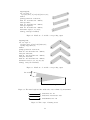
1
METAPOST
a user’s manual
John D. Hobby
and the MetaPost development team
documented version: 1.503
May 21, 2014
Contents
1 Introduction
1
2 Basic Drawing Statements
2
3 The MetaPost Workflow
3
4 Curves
4.1 Bézier Cubic Curves . . . . . . .
4.2 Specifying Direction, Tension,
and Curl . . . . . . . . . . . . . .
4.3 Summary of Path Syntax . . . .
5
6
9.7
9.8
Pens . . . . . . . . . . . . . . . .
Clipping and Low-Level Drawing Commands . . . . . . . . . .
9.9 Directing Output to a Picture
Variable . . . . . . . . . . . . . .
9.10 Inspecting the Components of a
Picture . . . . . . . . . . . . . . .
9.11 Decomposing the Glyphs of a Font
43
44
46
46
48
10 Macros
10.1 Grouping . . . . . . . . . . . . .
10.2 Parameterized Macros . . . . . .
10.3 Suffix and Text Parameters . . .
10.4 Vardef Macros . . . . . . . . . .
10.5 Defining Unary and Binary Macros
50
51
52
55
58
59
6 Expressions
14
6.1 Data Types . . . . . . . . . . . . 14
6.2 Operators . . . . . . . . . . . . . 15
6.3 Fractions, Mediation, and Unary
Operators . . . . . . . . . . . . . 17
11 Loops
61
12 Reading and Writing Files
62
7 Variables
18
7.1 Tokens . . . . . . . . . . . . . . . 19
7.2 Variable Declarations . . . . . . . 19
14 Another Look at the MetaPost
Workflow
65
14.1 Customizing Run-Time Behavior 65
14.2 Previewing PostScript Output . . 68
14.3 Debugging . . . . . . . . . . . . . 70
14.4 Importing MetaPost Graphics
into External Applications . . . . 73
7
10
5 Linear Equations
11
5.1 Equations and Coordinate Pairs . 11
5.2 Dealing with Unknowns . . . . . 13
8 Integrating Text and Graphics
8.1 Typesetting Your Labels . . .
8.2 Font Map Files . . . . . . . .
8.3 The infont Operator . . . .
8.4 Measuring Text . . . . . . . .
.
.
.
.
.
.
.
.
9 Advanced Graphics
9.1 Building Cycles . . . . . . . . . .
9.2 Dealing with Paths Parametrically
9.3 Affine Transformations . . . . . .
9.4 Dashed Lines . . . . . . . . . . .
9.5 Local specials . . . . . . . . . . .
9.6 Other Options . . . . . . . . . .
1
13 Utility Routines
63
13.1 TEX.mp . . . . . . . . . . . . . . . 63
21
22
26
26
27
A High-precision arithmetic with
MetaPost
28
30
32
35
37
40
40
77
B Reference Manual
78
B.1 The MetaPost Language . . . . . 78
B.2 Command-Line Syntax . . . . . . 97
C Legacy Information
100
C.1 MetaPost Versus METAFONT . . 100
C.2 File Name Templates . . . . . . . 103
Introduction
MetaPost is a programming language much like Knuth’s METAFONT1 [8] except that it outputs
either vector graphics in the Postscript or SVG formats or bitmap graphics in the PNG format.
Borrowed from METAFONT are the basic tools for creating and manipulating pictures. These include numbers, coordinate pairs, cubic splines, affine transformations, text strings, and boolean
quantities. Additional features facilitate integrating text and graphics and accessing special features
of PostScript2 such as clipping, shading, and dashed lines. Another feature borrowed from METAFONT is the ability to solve linear equations that are given implicitly, thus allowing many programs
to be written in a largely declarative style. By building complex operations from simpler ones,
MetaPost achieves both power and flexibility.
1 METAFONT
2 PostScript
is a trademark of Addison Wesley Publishing company.
is a trademark of Adobe Systems Inc.
1
MetaPost is particularly well-suited to generating figures for technical documents where some
aspects of a picture may be controlled by mathematical or geometrical constraints that are best
expressed symbolically. In other words, MetaPost is not meant to take the place of a freehand drawing tool or even an interactive graphics editor. It is really a programming language for generating
graphics, especially figures for TEX3 and troff documents.
This document introduces the MetaPost language, beginning with the features that are easiest
to use and most important for simple applications. The first few sections describe the language as
it appears to the novice user with key parameters at their default values. Some features described
in these sections are part of a predefined macro package called Plain. Later sections summarize the
complete language and distinguish between primitives and preloaded macros from the Plain macro
package. Reading the manual and creating moderately complex graphics with MetaPost does not
require knowledge of METAFONT or access to The METAFONTbook [8]. However, to really master
MetaPost, both are beneficial, since the MetaPost language is based on Knuth’s METAFONT to a
large extent. Appendix C.1 gives a detailed comparison of MetaPost and METAFONT.
MetaPost documentation is completed by “Drawing Boxes with MetaPost” and “Drawing Graphs
with MetaPost”—the manuals of the boxes and graph packages originally developed by John D.
Hobby.
The MetaPost home page is http://tug.org/metapost. It has links to much additional information, including many articles that have been written about MetaPost. For general help, try
the [email protected] mailing list; you can subscribe to this list at http://tug.org/mailman/
listinfo/metapost.
The development is currently hosted at http://foundry.supelec.fr/projects/metapost/;
visit this site for the current development team members, sources, and much else.
Please report bugs and request enhancements either on the [email protected] list, or through
the address given above. (Please do not send reports directly to Dr. Hobby any more.)
2
Basic Drawing Statements
The simplest drawing statement is the one that draws a single dot with the current pen at a given
coordinate:
drawdot (30,0)
MetaPost can also draw straight lines. Thus
draw (20,20)--(0,0)
draws a diagonal line and
draw (20,20)--(0,0)--(0,30)--(30,0)--(0,0)
draws a polygonal line like this:
What is meant by coordinates like (30,0)? MetaPost uses the same default coordinate system
that PostScript does. This means that (30,0) is 30 units to the right of the origin, where a unit
1
is 72
of an inch. We shall refer to this default unit as a PostScript point to distinguish it from the
1
standard printer’s point which is 72.27
inches.
MetaPost uses the same names for units of measure that TEX and METAFONT do. Thus bp refers
to PostScript points (“big points”) and pt refers to printer’s points. Other units of measure include
3T
EX is a trademark of the American Mathematical Society.
2
in for inches, pc for picas, cm for centimeters, mm for millimeters, cc for ciceros, and dd for Didot
points. For example,
(2cm,2cm)--(0,0)--(0,3cm)--(3cm,0)--(0,0)
generates a larger version of the above diagram. It is OK to say 0 instead 0cm because cm is really just
a conversion factor and 0cm just multiplies the conversion factor by zero. (MetaPost understands
constructions like 2cm as shorthand for 2*cm). The coordinate (0,0) can also be referred to as
origin, as in
drawdot origin
It is convenient to introduce your own scale factor, say 𝑢. Then you can define coordinates in
terms of 𝑢 and decide later whether you want to begin with u=1cm or u=0.5cm. This gives you
control over what gets scaled and what does not so that changing 𝑢 will not affect features such as
line widths.
There are many ways to affect the appearance of a line besides just changing its width, so the
width-control mechanisms allow a lot of generality that we do not need yet. This leads to the strange
looking statement
pickup pencircle scaled 4pt
for setting the line width (actually the pen size) for subsequent draw or drawdot statements to 4
points. (This is about eight times the default pen size).
With such a large pen size, the drawdot statement draws rather bold dots. We can use this to
make a grid of dots by nesting drawdot in a pair of loops:
for i=0 upto 2:
for j=0 upto 2: drawdot (i*u,j*u); endfor
endfor
The outer loop runs for 𝑖 = 0, 1, 2 and the inner loop runs for 𝑗 = 0, 1, 2. The result is a threeby-three grid of bold dots as shown in Figure 1. The figure also includes a larger version of the
polygonal line diagram that we saw before.
beginfig(2);
u=1cm;
draw (2u,2u)--(0,0)--(0,3u)--(3u,0)--(0,0);
pickup pencircle scaled 4pt;
for i=0 upto 2:
for j=0 upto 2: drawdot (i*u,j*u); endfor
endfor
endfig;
Figure 1: MetaPost commands and the resulting output
3
The MetaPost Workflow
Before describing the MetaPost language in detail, let’s have a look at MetaPost’s graphic design
workflow. This section also contains a few technical details about MetaPost’s compilation process,
just enough to get you started. Section 14 is more elaborate on this topic.
In this manual, we’ll assume a stand-alone command-line executable of the MetaPost compiler
is used, which is usually called mpost. The syntax and program name itself are system-dependent;
sometimes it is named mp. The executable is actually a small wrapper program around mplib, a
library containing the MetaPost compiler. The library can as well be embedded into third-party
applications.4 Section 14.4 has some brief information on how to use the MetaPost compiler built4C
API and Lua bindings are described in file manual/mplibapi.pdf as part of the MetaPost distribution.
3
Editor
Previewer
fig.1
fig.mp
fig.log
MetaPost
Figure 2: The basic MetaPost workflow
into LuaTEX. For more information, please refer to the documentation of the embedding application.
The basic MetaPost workflow is depicted in figure 2. Being a graphics description language,
creating graphics with MetaPost follows the edit-compile-debug paradigm known from other programming languages.
To create graphics with MetaPost, you prepare a text file containing code in the MetaPost
language and then invoke the compiler, usually by giving a command of the form
mpost ⟨input file⟩
on the command-line. MetaPost input files normally have names ending .mp but this part of the
name can be omitted when invoking MetaPost. A complete description of the command-line syntax
can be found in Section B.2.
Any terminal I/O during the compilation process is summarized in a transcript file called ⟨jobname⟩.log, where ⟨jobname⟩ is the base name of the input file. This includes error messages and
any MetaPost commands entered in interactive mode.
If all goes well during compilation, MetaPost outputs one or more graphic files in a variant of
the PostScript format, by default. PostScript output can be previewed with any decent PostScript
viewer, e.g., GSview or PS_View. Section 14.2 has some tips and discusses several more elaborate
ways for previewing PostScript output. Particularly, if graphics contain text labels, some more
work might be required to get robust results in a PostScript viewer. MetaPost is also capable of
generating graphics in the SVG and PNG formats. These file types can be previewed with certain
web browsers, for example Firefox 3 or Konqueror 4.2, or general purpose image viewers.
What does one do with all the graphic files? PostScript files are perfectly suitable for inclusion
into documents created by TEX or troff. The SVG format, as an XML descendant (Extensible
Meta Language), is more aiming at automated data processing/interchanging. The PNG format is
a losslessly compressing bitmap format. Both, SVG and PNG graphics, are widely used for web
applications. Section 14.4 deals with the import of MetaPost graphics into external applications.
4
A MetaPost input file normally contains a sequence of beginfig(), endfig pairs with an end
statement after the last one.5 These are macros that perform various administrative functions and
ensure that the results of all drawing operations get packaged up and translated into PostScript (or
the SVG or PNG format). The numeric argument to the beginfig macro determines the name of
the corresponding output file, whose name, by default, is of the form ⟨jobname⟩.⟨n⟩, where ⟨n⟩ is
the current argument to beginfig rounded to the nearest integer. As an example, if a file is named
fig.mp and contains the lines
beginfig(1);
⟨drawing statements⟩
endfig;
end
the output from statements between beginfig(1) and the next endfig is written in a file fig.1.
Statements can also appear outside beginfig . . . endfig. Such statements are processed, but
drawing operations generate no visible output. Typically, global configurations are put outside
beginfig . . . endfig, e.g., assignments to internal variables, such as outputtemplate, or a LATEX
preamble declaration for enhanced text rendering. Comments in MetaPost code are introduced by
the percent sign %, which causes the remainder of the current line to be ignored.
The remainder of this section briefly introduces three assignments to internal variables, each one
useful by itself, that can often be found in MetaPost input files:
prologues := 3;
outputtemplate := "%j-%c.mps";
outputformat := "svg";
If your graphics contain text labels, you might want to set variable prologues to 3 to make
sure the correct fonts are used under all possible circumstances. The second assignment changes the
output file naming scheme to the form ⟨jobname⟩-⟨n⟩.mps. That way, instead of a numeric index,
all output files get a uniform file extension mps, which is typically used for MetaPost’s PostScript
output. The last assignment lets MetaPost write output files in the SVG format rather than in the
PostScript format. More information can be found in Sections 8.1 and 14.
4
Curves
MetaPost is perfectly happy to draw curved lines as well as straight ones. A draw statement with
the points separated by .. draws a smooth curve through the points. For example consider the
result of
draw z0..z1..z2..z3..z4
after defining five points as follows:
z0 = (0,0);
z2 = (40,90);
z4 = (30,50);
z1 = (60,40);
z3 = (10,70);
Figure 3 shows the curve with points z0 through z4 labeled.
There are many other ways to draw a curved path through the same five points. To make a
smooth closed curve, connect z4 back to the beginning by appending ..cycle to the draw statement
as shown in Figure 4a. It is also possible in a single draw statement to mix curves and straight lines
as shown in Figure 4b. Just use -- where you want straight lines and .. where you want curves.
Thus
draw z0..z1..z2..z3--z4--cycle
5 Omitting
the final end statement causes MetaPost to enter interactive mode after processing the input file.
5
2
3
4
1
0
Figure 3: The result of draw z0..z1..z2..z3..z4
produces a curve through points 0, 1, 2, and 3, then a polygonal line from point 3 to point 4 and
back to point 0. The result is essentially the same as having two draw statements
draw z0..z1..z2..z3
and
draw z3--z4--z0
2
2
3
3
4
4
1
1
0
0
(𝑎)
(𝑏)
Figure 4: (a) The result of draw z0..z1..z2..z3..z4..cycle; (b) the result of draw z0..z1..
z2..z3–z4–cycle.
MetaPost already provides a small selection of basic path shapes that can be used to derive
custom paths from. The predefined variable fullcircle refers to a closed path describing a circle
of unit diameter centered on the origin. There are also halfcircle and quartercircle, the former
being the part of a full circle covering the first and second quadrant and the latter covering just the
first quadrant. Because of the mathematical model that is used to describe paths in MetaPost, all
these are not exactly circular paths, but very good approximations (see Figure 5).
Rectangularly shaped paths can be derived from unitsquare, a closed path describing a square
of unit side length whose lower left corner is located at the origin.
4.1
Bézier Cubic Curves
When MetaPost is asked to draw a smooth curve through a sequence of points, it constructs a
piecewise cubic curve with continuous slope and approximately continuous curvature. This means
that a path specification such as
z0..z1..z2..z3..z4..z5
6
Figure 5: A circle and a square with cardinal points. Arrows are pointing to the start and end points
of the closed paths.
results in a curve that can be defined parametrically as (𝑋(𝑡), 𝑌 (𝑡)) for 0 ≤ 𝑡 ≤ 5, where 𝑋(𝑡)
and 𝑌 (𝑡) are piecewise cubic functions. That is, there is a different pair of cubic functions for each
integer-bounded 𝑡-interval. If z0 = (𝑥0 , 𝑦0 ), z1 = (𝑥1 , 𝑦1 ), z2 = (𝑥2 , 𝑦2 ), . . . , MetaPost selects Bézier
− −
+
+ +
control points (𝑥+
0 , 𝑦0 ), (𝑥1 , 𝑦1 ), (𝑥1 , 𝑦1 ), . . . , where
𝑋(𝑡 + 𝑖)
=
−
2
3
(1 − 𝑡)3 𝑥𝑖 + 3𝑡(1 − 𝑡)2 𝑥+
𝑖 + 3𝑡 (1 − 𝑡)𝑥𝑖+1 + 𝑡 𝑥𝑖+1 ,
𝑌 (𝑡 + 𝑖)
=
−
(1 − 𝑡)3 𝑦𝑖 + 3𝑡(1 − 𝑡)2 𝑦𝑖+ + 3𝑡2 (1 − 𝑡)𝑦𝑖+1
+ 𝑡3 𝑦𝑖+1
for 0 ≤ 𝑡 ≤ 1. The precise rules for choosing the Bézier control points are described in [7] and in
The METAFONTbook [8].
In order for the path to have a continuous slope at (𝑥𝑖 , 𝑦𝑖 ), the incoming and outgoing directions
at (𝑋(𝑖), 𝑌 (𝑖)) must match. Thus the vectors
−
(𝑥𝑖 − 𝑥−
𝑖 , 𝑦𝑖 − 𝑦𝑖 )
and
+
(𝑥+
𝑖 − 𝑥𝑖 , 𝑦𝑖 − 𝑦𝑖 )
−
must have the same direction; i.e., (𝑥𝑖 , 𝑦𝑖 ) must be on the line segment between (𝑥−
𝑖 , 𝑦𝑖 ) and
+ +
(𝑥𝑖 , 𝑦𝑖 ). This situation is illustrated in Figure 6 where the Bézier control points selected by MetaPost are connected by dashed lines. For those who are familiar with the interesting properties of
this construction, MetaPost allows the control points to be specified directly in the following format:
draw (0,0)..controls
..(60,40)..controls
..(40,90)..controls
..(10,70)..controls
..(30,50);
(26.8,-1.8)
(67.1,61.0)
(25.4,94.0)
( 9.6,58.8)
and
and
and
and
(51.4,14.6)
(59.8,84.6)
(10.5,84.5)
(18.8,49.6)
For a way to extract the control points of a path, given by the user or calculated by MetaPost,
see section 9.2.
4.2
Specifying Direction, Tension, and Curl
MetaPost provides many ways of controlling the behavior of a curved path without actually specifying
the control points. For instance, some points on the path may be selected as vertical or horizontal
extrema. If z1 is to be a horizontal extreme and z2 is to be a vertical extreme, you can specify that
(𝑋(𝑡), 𝑌 (𝑡)) should go upward at z1 and to the left at z2:
draw z0..z1{up}..z2{left}..z3..z4;
The resulting shown in Figure 7 has the desired vertical and horizontal directions at z1 and z2,
but it does not look as smooth as the curve in Figure 3. The reason is the large discontinuity in
7
2
3
4
1
0
Figure 6: The result of draw z0..z1..z2..z3..z4 with the automatically-selected Bézier control
polygon illustrated by dashed lines.
curvature at z1. If it were not for the specified direction at z1, the MetaPost interpreter would have
chosen a direction designed to make the curvature above z1 almost the same as the curvature below
that point.
2
3
4
1
0
Figure 7: The result of draw z0..z1{up}..z2{left}..z3..z4.
How can the choice of directions at given points on a curve determine whether the curvature
will be continuous? The reason is that curves used in MetaPost come from a family where a path is
determined by its endpoints and the directions there. Figures 8 and 9 give a good idea of what this
family of curves is like.
beginfig(7)
for a=0 upto 9:
draw (0,0){dir 45}..{dir -10a}(6cm,0);
endfor
endfig;
Figure 8: A curve family and the MetaPost instructions for generating it
beginfig(8)
for a=0 upto 7:
draw (0,0){dir 45}..{dir 10a}(6cm,0);
endfor
endfig;
Figure 9: Another curve family with the corresponding MetaPost instructions
8
Figures 8 and 9 illustrate a few new MetaPost features. The first is the dir operator that takes
an angle in degrees and generates a unit vector in that direction. Thus dir 0 is equivalent to right
and dir 90 is equivalent to up. There are also predefined direction vectors left and down for dir
180 and dir 270.
The direction vectors given in {} can be of any length, and they can come before a point as well
as after one. It is even possible for a path specification to have directions given before and after a
point. For example a path specification containing
..{dir 60}(10,0){up}..
produces a curve with a corner at (10, 0).
Note that some of the curves in Figure 8 have points of inflection. This is necessary in order to
produce smooth curves in situations like Figure 4a, but it is probably not desirable when dealing
with vertical and horizontal extreme points as in Figure 10a. If z1 is supposed to be the topmost
point on the curve, this can be achieved by using ... instead of .. in the path specification as shown
in Figure 10b. The meaning of ... is “choose an inflection-free path between these points unless
the endpoint directions make this impossible.” (It would be possible to avoid inflections in Figure 8,
but not in Figure 9).
1
1
0
2
draw z0{up}..z1{right}..z2{down}
0
2
draw z0{up}...z1{right}...z2{down}
Figure 10: Two draw statements and the resulting curves.
Another way to control a misbehaving path is to increase the “tension” parameter. Using .. in
a path specification sets the tension parameter to the default value 1. If this makes some part of a
path a little too wild, we can selectively increase the tension. If Figure 11a is considered “too wild,”
a draw statement of the following form increases the tension between z1 and z2:
draw z0..z1..tension 1.3..z2..z3
This produces Figure 11b. For an asymmetrical effect like Figure 11c, the draw statement becomes
draw z0..z1..tension 1.5 and 1..z2..z3
The tension parameter can be less than one, but it must be at least 34 .
1
0
1
2
(𝑎)
3
0
2
(𝑏)
1
3
0
2
(𝑐)
3
Figure 11: Results of draw z0..z1..tension 𝛼 and 𝛽 ..z2..z3 for various 𝛼 and 𝛽: (a) 𝛼 = 𝛽 = 1;
(b) 𝛼 = 𝛽 = 1.3; (c) 𝛼 = 1.5, 𝛽 = 1.
MetaPost paths also have a parameter called “curl” that affects the ends of a path. In the absence
of any direction specifications, the first and last segments of a non-cyclic path are approximately
circular arcs as in the 𝑐 = 1 case of Figure 12. To use a different value for the curl parameter, specify
{curl c} for some other value of 𝑐. Thus
draw z0{curl c}..z1..{curl c}z2
sets the curl parameter for z0 and z2. Small values of the curl parameter reduce the curvature at
the indicated path endpoints, while large values increase the curvature as shown in Figure 12. In
particular, a curl value of zero makes the curvature approach zero.
9
2
2
2
2
1
1
1
1
0
𝑐=0
0
𝑐=1
0
𝑐=2
0
𝑐=∞
Figure 12: Results of draw z0{curl c}..z1..{curl c}z2 for various values of the curl parameter 𝑐.
4.3
Summary of Path Syntax
There are a few other features of MetaPost path syntax, but they are relatively unimportant. Since
METAFONT uses the same path syntax, interested readers can refer to [8, chapter 14]. The summary
of path syntax in Figure 13 includes everything discussed so far including the -- and ... constructions which [8] shows to be macros rather than primitives. A few comments on the semantics are in
order here: If there is a non-empty ⟨direction specifier⟩ before a ⟨path knot⟩ but not after it, or vice
versa, the specified direction (or curl amount) applies to both the incoming and outgoing path segments. A similar arrangement applies when a ⟨controls⟩ specification gives only one ⟨pair primary⟩.
Thus
..controls (30,20)..
is equivalent to
...controls (30,20) and (30,20)..
⟨path expression⟩ → ⟨path subexpression⟩
| ⟨path subexpression⟩⟨direction specifier⟩
| ⟨path subexpression⟩⟨path join⟩ cycle
⟨path subexpression⟩ → ⟨path knot⟩
| ⟨path expression⟩⟨path join⟩⟨path knot⟩
⟨path join⟩ → -| ⟨direction specifier⟩⟨basic path join⟩⟨direction specifier⟩
⟨direction specifier⟩ → ⟨empty⟩
| {curl ⟨numeric expression⟩}
| {⟨pair expression⟩}
| {⟨numeric expression⟩,⟨numeric expression⟩}
⟨basic path join⟩ → .. | ... | ..⟨tension⟩.. | ..⟨controls⟩..
⟨tension⟩ → tension⟨numeric primary⟩
| tension⟨numeric primary⟩and⟨numeric primary⟩
⟨controls⟩ → controls⟨pair primary⟩
| controls⟨pair primary⟩and⟨pair primary⟩
Figure 13: The syntax for path construction
A pair of coordinates like (30,20) or a z variable that represents a coordinate pair is what
Figure 13 calls a ⟨pair primary⟩. A ⟨path knot⟩ is similar except that it can take on other forms
such as a path expression in parentheses. Primaries and expressions of various types will be discussed
in full generality in Section 6.
10
5
Linear Equations
An important feature taken from METAFONT is the ability to solve linear equations so that programs
can be written in a partially declarative fashion. For example, the MetaPost interpreter can read
a+b=3; 2a=b+3;
and deduce that 𝑎 = 2 and 𝑏 = 1. The same equations can be written slightly more compactly by
stringing them together with multiple equal signs:
a+b = 2a-b = 3;
Whichever way you give the equations, you can then give the command
show a,b;
to see the values of a and b. MetaPost responds by typing
>> 2
>> 1
Note that = is not an assignment operator; it simply declares that the left-hand side equals
the right-hand side. Thus a=a+1 produces an error message complaining about an “inconsistent
equation.” The way to increase the value of a is to use the assignment operator := as follows:
a:=a+1;
In other words, := is for changing existing values while = is for giving linear equations to solve.
There is no restriction against mixing equations and assignment operations as in the following
example:
a = 2; b = a; a := 3; c = a;
After the first two equations set a and b equal to 2, the assignment operation changes a to 3 without
affecting b. The final value of c is 3 since it is equated to the new value of a. In general, an
assignment operation is interpreted by first computing the new value, then eliminating the old value
from all existing equations before actually assigning the new value.
5.1
Equations and Coordinate Pairs
MetaPost can also solve linear equations involving coordinate pairs. We have already seen many
trivial examples of this in the form of equations like
z1=(0,.2in)
Each side of the equation must be formed by adding or subtracting coordinate pairs and multiplying
or dividing them by known numeric quantities. Other ways of naming pair-valued variables will be
discussed later, but the z⟨number⟩ is convenient because it is an abbreviation for
(x⟨number⟩, y⟨number⟩)
This makes it possible to give values to z variables by giving equations involving their coordinates.
For instance, points z1, z2, z3, and z6 in Figure 14 were initialized via the following equations:
z1=-z2=(.2in,0);
x3=-x6=.3in;
x3+y3=x6+y6=1.1in;
11
Exactly the same points could be obtained by setting their values directly:
z1=(.2in,0);
z2=(-.2in,0);
z3=(.3in,.8in); z6=(-.3in,1.4in);
After reading the equations, the MetaPost interpreter knows the values of z1, z2, z3, and z6.
The next step in the construction of Figure 14 is to define points z4 and z5 equally spaced along
the line from z3 to z6. Since this operation comes up often, MetaPost has a special syntax for it.
This mediation construction
z4=1/3[z3,z6]
means that z4 is
1
3
of the way from 𝑧3 to 𝑧6; i.e.,
1
z4 = z3 + (z6 − z3).
3
Similarly
makes z5
z5=2/3[z3,z6]
2
3
of the way from 𝑧3 to 𝑧6.
beginfig(13);
z1=-z2=(.2in,0);
x3=-x6=.3in;
x3+y3=x6+y6=1.1in;
z4=1/3[z3,z6];
z5=2/3[z3,z6];
z20=whatever[z1,z3]=whatever[z2,z4];
z30=whatever[z1,z4]=whatever[z2,z5];
z40=whatever[z1,z5]=whatever[z2,z6];
draw z1--z20--z2--z30--z1--z40--z2;
pickup pencircle scaled 1pt;
draw z1--z2;
draw z3--z6;
endfig;
40
20
30
6
3
2
1
Figure 14: MetaPost commands and the resulting figure. Point labels have been added to the figure
for clarity.
Mediation can also be used to say that some point is at an unknown position along the line
between two known points. For instance, we could a introduce new variable aa and write something
like
z20=aa[z1,z3];
This says that z20 is some unknown fraction aa of the way along the line between z1 and z3.
Another such equation involving a different line is sufficient to fix the value of z20. To say that z20
is at the intersection of the z1-z3 line and the z2-z4 line, introduce another variable ab and set
z20=ab[z2,z4];
This allows MetaPost to solve for x20, y20, aa, and ab.
It is a little painful to keep thinking up new names like aa and ab. This can be avoided by using
a special feature called whatever. This macro generates a new anonymous variable each time it
appears. Thus the statement
z20=whatever[z1,z3]=whatever[z2,z4]
12
sets z20 as before, except it uses whatever to generate two different anonymous variables instead
of aa and ab. This is how Figure 14 sets z20, z30, and z40.
5.2
Dealing with Unknowns
A system of equations such as those used in Figure 14 can be given in any order as long as all the
equations are linear and all the variables can be determined before they are needed. This means
that the equations
z1=-z2=(.2in,0);
x3=-x6=.3in;
x3+y3=x6+y6=1.1in;
z4=1/3[z3,z6];
z5=2/3[z3,z6];
suffice to determine z1 through z6, no matter what order the equations are given in. On the other
hand
z20=whatever[z1,z3]
is legal only when a known value has previously been specified for the difference z3 − z1, because
the equation is equivalent to
z20 = z1 + whatever*(z3-z1)
and the linearity requirement disallows multiplying unknown components of z3 − z1 by the anonymous unknown result of whatever. The general rule is that you cannot multiply two unknown
quantities or divide by an unknown quantity, nor can an unknown quantity be used in a draw
statement. Since only linear equations are allowed, the MetaPost interpreter can easily solve the
equations and keep track of what values are known.
The most natural way to ensure that MetaPost can handle an expression like
whatever[z1,z3]
is to ensure that z1 and z3 are both known. However this is not actually required since MetaPost
may be able to deduce a known value for z3 − z1 before either of z1 and z3 are known. For instance,
MetaPost will accept the equations
z3=z1+(.1in,.6in);
z20=whatever[z1,z3];
but it will not be able to determine any of the components of z1, z3, or z20.
These equations do give partial information about z1, z3, and z20. A good way to see this is to
give another equation such as
x20-x1=(y20-y1)/6;
This produces the error message “! Redundant equation.” MetaPost assumes that you are trying
to tell it something new, so it will usually warn you when you give a redundant equation. If the new
equation had been
(x20-x1)-(y20-y1)/6=1in;
the error message would have been
! Inconsistent equation (off by 71.99979).
This error message illustrates roundoff error in MetaPost’s linear equation solving mechanism.
Roundoff error is normally not a serious problem, but it is likely to cause trouble if you are trying
to do something like find the intersection of two lines that are almost parallel.
13
6
Expressions
It is now time for a more systematic view of the MetaPost language. We have seen that there
are numeric quantities and coordinate pairs, and that these can be combined to specify paths for
draw statements. We have also seen how variables can be used in linear equations, but we have not
discussed all the operations and data types that can be used in equations.
It is possible to experiment with expressions involving any of the data types mentioned below
by using the statement
show ⟨expression⟩
to ask MetaPost to print a symbolic representation of the value of each expression. For known
numeric values, each is printed on a new line preceded by “>> ”. Other types of result are printed
similarly, except that complicated values are sometimes not printed on standard output. This
produces a reference to the transcript file that looks like this:
>> picture (see the transcript file)
If you want to the full results of show statements to be printed on your terminal, assign a positive
value to the internal variable tracingonline.
6.1
Data Types
MetaPost actually has ten basic data types: numeric, pair, path, transform, (rgb)color, cmykcolor,
string, boolean, picture, and pen. Let us consider these one at a time beginning with the numeric
type.
Numeric quantities in MetaPost are represented in fixed point arithmetic as integer multiples
1
, the smallest positive value, which is also available as the predefined constant epsilon.6
of 65536
Numeric quantities must normally have absolute values less than 4096 but intermediate results can
be eight times larger. This should not be a problem for distances or coordinate values since 4096
PostScript points is more than 1.4 meters. If you need to work with numbers of magnitude 4096
or more, setting the internal variable warningcheck to zero suppresses the warning messages about
large numeric quantities.
The pair type is represented as a pair of numeric quantities. We have seen that pairs are used to
give coordinates in draw statements. Pairs can be added, subtracted, used in mediation expressions,
or multiplied or divided by numerics.
Paths have already been discussed in the context of draw statements, but that discussion did not
mention that paths are first-class objects that can be stored and manipulated. A path represents a
straight or curved line that is defined parametrically.
Another data type represents an arbitrary affine transformation. A transform can be any combination of rotating, scaling, slanting, and shifting. If p = (𝑝𝑥 , 𝑝𝑦 ) is a pair and T is a transform,
p transformed T
is a pair of the form
(𝑡𝑥 + 𝑡𝑥𝑥 𝑝𝑥 + 𝑡𝑥𝑦 𝑝𝑦 , 𝑡𝑦 + 𝑡𝑦𝑥 𝑝𝑥 + 𝑡𝑦𝑦 𝑝𝑦 ),
where the six numeric quantities (𝑡𝑥 , 𝑡𝑦 , 𝑡𝑥𝑥 , 𝑡𝑥𝑦 , 𝑡𝑦𝑥 , 𝑡𝑦𝑦 ) determine T. Transforms can also be applied
to paths, pictures, pens, and transforms.
The color type is like the pair type, except that it has three components instead of two and
each component is normally between 0 and 1. Like pairs, colors can be added, subtracted, used in
mediation expressions, or multiplied or divided by numerics. Colors can be specified in terms of the
predefined constants black, white, red, green, blue, or the red, green, and blue components can
6 MetaPost can also do arithmetic with higher and (almost) arbitrary precision.
information.
14
See Appendix A for more
be given explicitly. Black is (0,0,0) and white is (1,1,1). A level of gray such as (.4,.4,.4)
can also be specified as 0.4white. Although color typed variables may be any ordered triplet, when
adding an object to a picture, MetaPost will convert its color by clipping each component between
0 and 1. For example, MetaPost will output the color (1,2,3) as (1,1,1). MetaPost solves linear
equations involving colors the same way it does for pairs. The type ‘rgbcolor’ is an alias of type
‘color’.
The cmykcolor type is similar to the color type except that it has four components instead of
three. This type is used to specify colors by their cyan, magenta, yellow, and black components
explicitly. Because CMYK colors deal with pigments instead of light rays, the color white would be
expressed as (0,0,0,0) and black as (0,0,0,1). In theory, the colors (𝑐,𝑚,𝑦,1) and (1,1,1,𝑘)
should result in black for any values of 𝑐, 𝑚, 𝑦 and 𝑘, too. But in practice, this is avoided since it
is a waste of colored ink and can lead to unsatisfactory results.
A string represents a sequence of characters. String constants are given in double quotes
"like this". String constants cannot contain double quotes or newlines, but there is a way to
construct a string containing any sequence of eight-bit characters.
Conversion from strings to other types, notably numeric, can be accomplished by the scantokens
primitive:
n := scantokens(str);
More generally, scantokens parses a string into a token sequence, as if MetaPost had read it as
input.
The boolean type has the constants true and false and the operators and, or, not. The relations
= and <> test objects of any type for equality and inequality. Comparison relations <, <=, >, and
>= are defined lexicographically for strings and in the obvious way for numerics. Ordering relations
are also defined for booleans, pairs, colors, and transforms, but the comparison rules are not worth
discussing here.
The picture data type is just what the name implies. Anything that can be drawn in MetaPost
can be stored in a picture variable. In fact, the draw statement actually stores its results in a special
picture variable called currentpicture. Pictures can be added to other pictures and operated on
by transforms.
Finally, there is a data type called a pen. The main function of pens in MetaPost is to determine
line thickness, but they can also be used to achieve calligraphic effects. The statement
pickup ⟨pen expression⟩
causes the given pen to be used in subsequent draw or drawdot statements. Normally, the pen
expression is of the form
pencircle scaled ⟨numeric primary⟩.
This defines a circular pen that produces lines of constant thickness. If calligraphic effects are
desired, the pen expression can be adjusted to give an elliptical pen or a polygonal pen.
6.2
Operators
There are many different ways to make expressions of the ten basic types, but most of the operations
fit into a fairly simple syntax with four levels of precedence as shown in Figure 15. There are
primaries, secondaries, tertiaries, and expressions of each of the basic types, so the syntax rules
could be specialized to deal with items such as ⟨numeric primary⟩, ⟨boolean tertiary⟩, etc. This
allows the result type for an operation to depend on the choice of operator and the types of its
operands. For example, the < relation is a ⟨tertiary binary⟩ that can be applied to a ⟨numeric
expression⟩ and a ⟨numeric tertiary⟩ to give a ⟨boolean expression⟩. The same operator can accept
other operand types such as ⟨string expression⟩ and ⟨string tertiary⟩, but an error message results
if the operand types do not match.
15
⟨primary⟩ → ⟨variable⟩
| (⟨expression⟩)
| ⟨nullary op⟩
| ⟨of operator⟩⟨expression⟩of⟨primary⟩
| ⟨unary op⟩⟨primary⟩
⟨secondary⟩ → ⟨primary⟩
| ⟨secondary⟩⟨primary binop⟩⟨primary⟩
⟨tertiary⟩ → ⟨secondary⟩
| ⟨tertiary⟩⟨secondary binop⟩⟨secondary⟩
⟨expression⟩ → ⟨tertiary⟩
| ⟨expression⟩⟨tertiary binop⟩⟨tertiary⟩
Figure 15: The overall syntax rules for expressions
The multiplication and division operators * and / are examples of what Figure 15 calls a ⟨primary
binop⟩. Each can accept two numeric operands or one numeric operand and one operand of type pair
or color. The exponentiation operator ** is a ⟨primary binop⟩ that requires two numeric operands.
Placing this at the same level of precedence as multiplication and division has the unfortunate
consequence that 3*a**2 means (3𝑎)2 , not 3(𝑎2 ). Since unary negation applies at the primary level,
it also turns out that -a**2 means (−𝑎)2 . Fortunately, subtraction has lower precedence so that
a-b**2 does mean 𝑎 − (𝑏2 ) instead of (𝑎 − 𝑏)2 .
Another ⟨primary binop⟩ is the dotprod operator that computes the vector dot product of two
pairs. For example, z1 dotprod z2 is equivalent to x1*x2 + y1*y2.
The additive operators + and - are ⟨secondary binops⟩ that operate on numerics, pairs, or colors
and produce results of the same type. Other operators that fall
√ in this category are “Pythagorean
√
addition” ++ and “Pythagorean subtraction” +-+: a++b means 𝑎2 + 𝑏2 and a+-+b means 𝑎2 − 𝑏2 .
There are too many other operators to list here, but some of the most important are the boolean
operators and and or. The and operator is a ⟨primary binop⟩ and the or operator is a ⟨secondary
binop⟩.
The basic operations on strings are concatenation, substring construction and calculating the
length of a string. The ⟨tertiary binop⟩ & implements concatenation; e.g.,
"abc" & "de"
produces the string "abcde". The length operator returns the number of characters in a string if
the argument is a ⟨string primary⟩; e.g.,
length "abcde"
returns 5. Another application of the length operator is discussed on p. 33. For substring construction, the ⟨of operator⟩ substring is used like this:
substring ⟨pair expression⟩ of ⟨string primary⟩
The ⟨pair expression⟩ determines what part of the string to select. For this purpose, the string is
indexed so that integer positions fall between characters. Pretend the string is written on a piece of
graph paper so that the first character occupies 𝑥 coordinates between zero and one and the next
character covers the range 1 ≤ 𝑥 ≤ 2, etc. Thus the string "abcde" should be thought of like this
x=0
a b c d e
1
2
3
16
4
5
and substring (2,4) of "abcde" is "cd". This takes a little getting used to but it tends to avoid
annoying “off by one” errors.
Some operators take no arguments at all. An example of what Figure 15 calls a ⟨nullary op⟩ is
nullpicture which returns a completely blank picture.
The basic syntax in Figure 15 only covers aspects of the expression syntax that are relatively
type-independent. For instance, the complicated path syntax given in Figure 13 gives alternative
rules for constructing a ⟨path expression⟩. An additional rule
⟨path knot⟩ → ⟨pair tertiary⟩ | ⟨path tertiary⟩
explains the meaning of ⟨path knot⟩ in Figure 13. This means that the path expression
z1+(1,1){right}..z2
does not need parentheses around z1+(1,1).
6.3
Fractions, Mediation, and Unary Operators
Mediation expressions do not appear in the basic expression syntax of Figure 15. Mediation expressions are parsed at the ⟨primary⟩ level, so the general rule for constructing them is
⟨primary⟩ → ⟨numeric atom⟩[⟨expression⟩,⟨expression⟩]
where each ⟨expression⟩ can be of type numeric, pair, or color. The ⟨numeric atom⟩ in a mediation
expression is an extra simple type of ⟨numeric primary⟩ as shown in Figure 16. The meaning of all
this is that the initial parameter in a mediation expression needs to be parenthesized when it is not
just a variable, a positive number, or a positive fraction. For example,
-1[a,b] and (-1)[a,b]
are very different: the former is −𝑏 since it is equivalent to -(1[a,b]); the latter is 𝑎 − (𝑏 − 𝑎) or
2𝑎 − 𝑏.
⟨numeric primary⟩ → ⟨numeric atom⟩
| ⟨numeric atom⟩[⟨numeric expression⟩,⟨numeric expression⟩]
| ⟨of operator⟩⟨expression⟩of⟨primary⟩
| ⟨unary op⟩⟨primary⟩
⟨numeric atom⟩ → ⟨numeric variable⟩
| ⟨number or fraction⟩
| (⟨numeric expression⟩)
| ⟨numeric nullary op⟩
⟨number or fraction⟩ → ⟨number⟩/⟨number⟩
| ⟨number not followed by ‘/⟨number⟩’⟩
Figure 16: Syntax rules for numeric primaries
A noteworthy feature of the syntax rules in Figure 16 is that the / operator binds most tightly
when its operands are numbers. Thus 2/3 is a ⟨numeric atom⟩ while (1+1)/3 is only a ⟨numeric
secondary⟩. Applying a ⟨unary op⟩ such as sqrt makes the difference clear:
sqrt 2/3
means
√︁
2
3
while
sqrt(1+1)/3
17
√
means 2/3. Operators such as sqrt can be written in standard functional notation, but it is often
unnecessary to parenthesize the argument. This applies to any function that is parsed as a ⟨unary
op⟩. For instance abs(x) and abs x both compute the absolute value of x. The same holds for the
round, floor, ceiling, sind, and cosd functions. The last two of these compute trigonometric
functions of angles in degrees.
Not all unary operators take numeric arguments and return numeric results. For instance, the
abs operator can be applied to a pair to compute the Euclidean length of a vector. Applying the
unitvector operator to a pair produces the same pair rescaled so that its Euclidean length is 1. The
decimal operator takes a number and returns the string representation. The angle operator takes
a pair and computes the two-argument arctangent; i.e., angle is the inverse of the dir operator
that was discussed in Section 4.2. There is also an operator cycle that takes a ⟨path primary⟩ and
returns a boolean result indicating whether the path is a closed curve.
There is a whole class of other operators that classify expressions and return boolean results. A
type name such as pair can operate on any type of ⟨primary⟩ and return a boolean result indicating
whether the argument is a pair. Similarly, each of the following can be used as a unary operator:
numeric, boolean, cmykcolor, color, string, transform, path, pen, picture, and rgbcolor.
Besides just testing the type of a ⟨primary⟩, you can use the known and unknown operators to test
if it has a completely known value.
Even a number can behave like an operator in some contexts. This refers to the trick that allows
3x and 3cm as alternatives to 3*x and 3*cm. The rule is that a ⟨number or fraction⟩ that is not
followed by +, -, or another ⟨number or fraction⟩ can serve as a ⟨primary binop⟩. Thus 2/3x is two
2
and 3 3 is illegal.
thirds of x but (2)/3x is 3𝑥
There are also operators for extracting numeric subfields from pairs, colors, cmykcolors, and even
transforms. If p is a ⟨pair primary⟩, xpart p and ypart p extract its components so that
(xpart p, ypart p)
is equivalent to p even if p is an unknown pair that is being used in a linear equation. Similarly, a
color c is equivalent to
(redpart c, greenpart c, bluepart c).
For a cmykcolor c, the components are
(cyanpart c, magentapart c, yellowpart c, blackpart c)
and for a greyscale color c, there is only one component
greypart c.
All color component operators are discussed in more detail in section 9.10. Part specifiers for
transforms are discussed in section 9.3.
7
Variables
MetaPost allows compound variable names such as z.a, x2r, y2r, and z2r, where z2r means
(x2r,y2r) and z.a means (x.a,y.a). In fact there is a broad class of suffixes such that z⟨suffix⟩ means
(𝑥⟨suffix⟩, 𝑦⟨suffix⟩).
Since a ⟨suffix⟩ is composed of tokens, it is best to begin with a few comments about tokens.
18
ABCDEFGHIJKLMNOPQRSTUVWXYZ_abcdefghijklmnopqrstuvwxyz
:<=>|
#&@$
/*\
+!?
’‘
^~
{}
[
]
Table 1: Character classes for tokenization
7.1
Tokens
A MetaPost input file is treated as a sequence of numbers, string constants, and symbolic tokens. A
number consists of a sequence of digits possibly containing a decimal point. Technically, the minus
sign in front of a negative number is a separate token. Since MetaPost uses fixed point arithmetic,
it does not understand exponential notation such as 6.02E23. MetaPost would interpret this as the
number 6.02, followed by the symbolic token E, followed by the number 23.
Anything between a pair of double quotes " is a string constant. It is illegal for a string constant
to start on one line and end on a later line. Nor can a string constant contain double quotes " or
anything other than printable ASCII characters.
Everything in a line of input other than numbers and string constants is broken into symbolic
tokens. A symbolic token is a sequence of one or more similar characters, where characters are
“similar” if they occur on the same row of Table 1.
Thus A_alpha and +-+ are symbolic tokens but != is interpreted as two tokens and x34 is a
symbolic token followed by a number. Since the brackets [ and ] are listed on lines by themselves,
the only symbolic tokens involving them are [, [[, [[[, etc. and ], ]], etc.
Some characters are not listed in Table 1 because they need special treatment. The four characters
,;() are “loners”: each comma, semicolon, or parenthesis is a separate token even when they occur
consecutively. Thus (()) is four tokens, not one or two. The percent sign is very special because it
introduces comments. The percent sign and everything after it up to the end of the line are ignored.
Another special character is the period. Two or more periods together form a symbolic token,
but a single period is ignored, and a period preceded or followed by digits is part of a number Thus
.. and ... are symbolic tokens while a.b is just two tokens a and b. It conventional to use periods
to separate tokens in this fashion when naming a variable that is more than one token long.
7.2
Variable Declarations
A variable name is a symbolic token or a sequence of symbolic tokens. Most symbolic tokens are
legitimate variable names, but anything with a predefined meaning like draw, +, or .. is disallowed;
i.e., variable names cannot be macros or MetaPost primitives. This minor restriction allows an
amazingly broad class of variable names: alpha, ==>, @&#$&, and ~~ are all legitimate variable
names. Such symbolic tokens without special meanings are called tags.
A variable name can be a sequence of tags like f.bot or f.top. The idea is to provide some of
the functionality of Pascal records or C structures. It is also possible to simulate arrays by using
variable names that contain numbers as well as symbolic tokens. For example, the variable name
x2r consists of the tag x, the number 2, and the tag r. There can also be variables named x3r and
even x3.14r. These variables can be treated as an array via constructions like x[i]r, where i has
an appropriate numeric value. The overall syntax for variable names is shown in Figure 17.
19
⟨variable⟩ → ⟨tag⟩⟨suffix⟩
⟨suffix⟩ → ⟨empty⟩ | ⟨suffix⟩⟨subscript⟩ | ⟨suffix⟩⟨tag⟩
⟨subscript⟩ → ⟨number⟩ | [⟨numeric expression⟩]
Figure 17: The syntax for variable names.
Variables like x2 and y2 take on numeric values by default, so we can use the fact that z⟨suffix⟩
is an abbreviation for
(𝑥⟨suffix⟩, 𝑦⟨suffix⟩)
to generate pair-valued variables when needed. It turns out that the beginfig macro wipes out
pre-existing values variables that begin with the tags x or y so that beginfig . . . endfig blocks do
not interfere with each other when this naming scheme is used. In other words, variables that start
with x, y, z are local to the figure they are used in. General mechanisms for making variables local
will be discussed in Section 10.1.
Type declarations make it possible to use almost any naming scheme while still wiping out any
previous value that might cause interference. For example, the declaration
pair pp, a.b;
makes pp and a.b unknown pairs. Such a declaration is not strictly local since pp and a.b are not
automatically restored to their previous values at the end of the current figure. Of course, they are
restored to unknown pairs if the declaration is repeated.
Declarations work the same way for any of the other nine types: numeric, path, transform, color,
cmykcolor, string, boolean, picture, and pen. The only restriction is that you cannot give explicit
numeric subscripts in a variable declaration. Do not give the illegal declaration
numeric q1, q2, q3;
use the generic subscript symbol [] instead, to declare the whole array:
numeric q[];
You can also declare “multidimensional” arrays. After the declaration
path p[]q[], pq[][];
p2q3 and pq1.4 5 are both paths.
Internal variables like tracingonline cannot be declared in the normal fashion. All the internal
variables discussed in this manual are predefined and do not have to be declared at all, but there is a
way to declare that a variable should behave like a newly-created internal variable. The declaration
is newinternal followed by an optional type specifier numeric or string and a list of symbolic
tokens. For example,
newinternal numeric n, m;
newinternal string s, t;
newinternal num;
are valid declarations that declare three internal numeric variables n, m, and num and two internal
string variables s and t.
Internal variables always have known values, and these values can only be changed by using the
assignment operator :=. Internal numeric variables are initially zero and internal string variables
are initially the empty string "", except that the Plain macro package gives some of the variables
different initial values. (The Plain macros are normally preloaded automatically as explained in
Section 1.)
20
Internal string variables have been introduced in MetaPost version 1.200. For backwards compatibility, if the type specifier is missing, internal variables default to a numeric type, as in the
last example. The declarations newinternal numeric; and newinternal string; are invalid and
throw an error.
8
Integrating Text and Graphics
MetaPost has a number of features for including labels and other text in the figures it generates.
The simplest way to do this is to use the label statement
label⟨label suffix⟩(⟨string or picture expression⟩, ⟨pair expression⟩);
The ⟨string or picture expression⟩ gives the label and the ⟨pair expression⟩ says where to put it.
The ⟨label suffix⟩ can be ⟨empty⟩ in which case the label is just centered on the given coordinates.
If you are labeling some feature of a diagram you probably want to offset the label slightly to avoid
overlapping. This is illustrated in Figure 18 where the "a" label is placed above the midpoint of the
line it refers to and the "b" label is to the left of the midpoint of its line. This is achieved by using
label.top for the "a" label and label.lft for the "b" label as shown in the figure. The ⟨label
suffix⟩ specifies the position of the label relative to the specified coordinates. The complete set of
possibilities is
⟨label suffix⟩ → ⟨empty⟩ | lft | rt | top | bot | ulft | urt | llft | lrt
where lft and rt mean left and right and llft, ulft, etc. mean lower left, upper left, etc. The
actual amount by which the label is offset in whatever direction is determined by the internal variable
labeloffset.
beginfig(17);
a=.7in; b=.5in;
z0=(0,0);
z1=-z3=(a,0);
z2=-z4=(0,b);
draw z1..z2..z3..z4..cycle;
draw z1--z0--z2;
label.top("a", .5[z0,z1]);
label.lft("b", .5[z0,z2]);
dotlabel.bot("(0,0)", z0);
endfig;
b
a
(0,0)
Figure 18: MetaPost code and the resulting output
Figure 18 also illustrates the dotlabel statement. This is effectively like a label statement
followed by a statement drawing a dot at the indicated coordinates. For example
dotlabel.bot("(0,0)", z0)
places a dot at z0 and then puts the label “(0,0)” just below the dot. The diameter of the dot
drawn by the dotlabel statement is determined by the value of the internal variable dotlabeldiam.
Default value is 3bp.
Another alternative is the macro thelabel. This has the same syntax as the label and dotlabel
statements except that it returns the label as a ⟨picture primary⟩ instead of actually drawing it.
Thus
label.bot("(0,0)", z0)
21
is equivalent to
draw thelabel.bot("(0,0)", z0)
For simple applications of labeled figures, you can normally get by with just label and dotlabel.
In fact, you may be able to use a short form of the dotlabel statement that saves a lot of typing
when you have many points z0, z1, z.a, z.b, etc. and you want to use the z suffixes as labels. The
statement
dotlabels.rt(0, 1, a);
is equivalent to
dotlabel.rt("0",z0); dotlabel.rt("1",z1); dotlabel.rt("a",z.a);
Thus the argument to dotlabels is a list of suffixes for which z variables are known, and the ⟨label
suffix⟩ given with dotlabels is used to position all the labels.
There is also a labels statement that is analogous to dotlabels but its use is discouraged
because it presents compatibility problems with METAFONT. Some versions of the preloaded Plain
macro package define labels to be synonymous with dotlabels.
For labeling statements such as label and dotlabel that use a string expression for the label
text, the string gets typeset in a default font as determined by the string variable defaultfont.
The initial value of defaultfont is likely to be "cmr10", but it can be changed to a different font
name by giving an assignment such as
defaultfont:="ptmr8r"
ptmr8r is a typical way to refer to the Times-Roman font in TEX. The discussion of font names on
p. 22 explains further.
There is also a numeric quantity called defaultscale that determines the type size. When
defaultscale is 1, you get the “normal size” which is usually 10 point, but this can also be changed.
For instance
defaultscale := 1.2
makes labels come out twenty percent larger. If you do not know the normal size and you want to
be sure the text comes out at some specific size, say 12 points, you can use the fontsize operator
to determine the normal size: e.g.,
defaultscale := 12pt/fontsize defaultfont;
When you change defaultfont, the new font name should be something that TEX would understand since MetaPost gets height and width information by reading a tfm file. (This is explained in
The TEXbook [9].) It should be possible to use built-in PostScript fonts, but the names for them are
system-dependent. Some typical ones are ptmr8r for Times-Roman, pplr8r for Palatino, and phvr
for Helvetica. The Fontname document, available at http://tug.org/fontname, has much more
information about font names and TEX. A TEX font such as cmr10 is a little dangerous because it
does not have a space character or certain ASCII symbols.
MetaPost does not use the ligatures and kerning information that comes with a TEX font. Further,
MetaPost itself does not interpret virtual fonts.
8.1
Typesetting Your Labels
TEX may be used to format complex labels. If you say
btex ⟨typesetting commands⟩ etex
22
in a MetaPost input file, the ⟨typesetting commands⟩ get processed by TEX and translated into a
picture expression (actually a ⟨picture primary⟩) that can be used in a label or dotlabel statement.
Any spaces after btex or before etex are ignored. For instance, the statement
label.lrt(btex $\sqrt x$ etex, (3,sqrt 3)*u)
√
in Figure 19 places the label 𝑥 at the lower right of the point (3,sqrt 3)*u.
beginfig(18);
numeric u;
u = 1cm;
draw (0,2u)--(0,0)--(4u,0);
pickup pencircle scaled 1pt;
draw (0,0){up}
for i=1 upto 8: ..(i/2,sqrt(i/2))*u endfor;
label.lrt(btex $\sqrt x$ etex, (3,sqrt 3)*u);
label.bot(btex $x$ etex, (2u,0));
label.lft(btex $y$ etex, (0,u));
endfig;
√
x
y
x
Figure 19: Arbitrary TEX as labels
Figure 20 illustrates some of the more complicated things that can be done with labels. Since the
result of btex . . . etex is a picture, it can be operated on like a picture. In particular, it is possible
to apply transformations to pictures. We have not discussed the syntax for this yet, but a ⟨picture
secondary⟩ can be
⟨picture secondary⟩ rotated ⟨numeric primary⟩
This is used in Figure 20 to rotate the label “𝑦 axis” so that it runs vertically.
y=
2
1 + cos x
y axis
beginfig(19);
numeric ux, uy;
120ux=1.2in; 4uy=2.4in;
draw (0,4uy)--(0,0)--(120ux,0);
pickup pencircle scaled 1pt;
draw (0,uy){right}
for ix=1 upto 8:
..(15ix*ux, uy*2/(1+cosd 15ix))
endfor;
label.bot(btex $x$ axis etex, (60ux,0));
label.lft(btex $y$ axis etex rotated 90,
(0,2uy));
label.lft(
btex $\displaystyle y={2\over1+\cos x}$ etex,
(120ux, 4uy));
endfig;
x axis
Figure 20: TEX labels with display math, and rotated by MetaPost
Another complication in Figure 20 is the use of the displayed equation
𝑦=
2
1 + cos 𝑥
23
as a label. It would be more natural to code this as
$$y={2\over 1+\cos x}$$
but this would not work because TEX typesets the labels in “horizontal mode.”
For a way to typeset variable text as labels, see the TEX utility routine described on p. 63.
Here is how TEX material gets translated into a form MetaPost understands: MetaPost stores
all btex . . . etex blocks in a temporary file and then runs TEX on that file. If the environment
variable MPTEXPRE is set to the name of an existing file, its content will be prepended to the output
file for processing by TEX. You can use this to include LATEX preambles, for instance. The TEX
macro described on p. 63 provides another way to handle this.
Once the TEX run is finished, MetaPost translates the resulting DVI file into low level MetaPost
commands that are then read instead of the btex . . . etex blocks. If the main file is fig.mp, the
translated TEX material is placed in a file named fig.mpx.
The conversion normally runs silently without any user intervention but it could fail, for instance
if one of the btex . . . etex blocks contains an erroneous TEX command. In that case, the TEX input
is saved in the file mpxerr.tex and the TEX error messages appear in mpxerr.log.
The DVI to MetaPost conversion route does understand virtual fonts, so you can use your normal
TEX font switching commands inside the label.
In MetaPost versions before 1.100, the TEX label preprocessing was handled by an external program that was called upon automatically by MetaPost. On Web2C-based systems, the preprocessor
was normally named makempx, which called the utility mpto for the creation of the TEX input file
and the utility dvitomp for the conversion to low level MetaPost. In the current MetaPost version,
the work of this program is now done internally. However, if the environment variable MPXCOMMAND is
set, the whole label conversion mechanism will be delegated to the command given in that variable.
TEX macro definitions or any other auxiliary TEX commands can be enclosed in a verbatimtex
. . . etex block. The difference between btex and verbatimtex is that the former generates a picture
expression while the latter only adds material for TEX to process. For instance, if you want TEX to
typeset labels using macros defined in mymac.tex, your MetaPost input file would look something
like this:
verbatimtex \input mymac etex
beginfig(1);
...
label(btex ⟨TEX material using mymac.tex⟩ etex, ⟨some coordinates⟩);
...
On Unix7 and other Web2C-based systems, the option -troff to MetaPost tells the preprocessor
that btex . . . etex and verbatimtex . . . etex blocks are in troff instead of TEX. When using this
option, MetaPost sets the internal variable troffmode to 1.
Setting prologues can be useful with TEX, too, not just troff. Here is some explanation:
• In PostScript output mode, when prologues is 0, which is the default, the MetaPost output
files do not have embedded fonts. Fonts in the resulting output will probably render as Courier
or Times-Roman.
In SVG mode, the text will probably render in a generic sans serif font. There may very well
be problems with the encoding of non-ASCII characters: the font model of SVG is totally
different from the model used by MetaPost.
• In PostScript output mode, when prologues is 1, the MetaPost output claims to be “structured
PostScript” (EPSF), but it is not completely conformant. This variant is kept for backward
7 Unix
is a registered trademark of Unix Systems Laboratories.
24
compatibility with old (troff) documents, but its use is deprecated. MetaPost sets prologues
to 1 when the -troff option is given on the command line.
A prologues:=1 setting is currently ignored in SVG output mode. The value is reserved for
future use (possibly for mapping to font-family, font-weight, etc. properties).
• In PostScript output mode, when prologues is 2, the MetaPost output is EPSF and assumes
that the text comes from PostScript fonts provided by the “environment”, such as the document
viewer or embedded application using the output. MetaPost will attempt to set up the font
encodings correctly, based on fontmapfile and fontmapline commands.
A prologues:=2 setting is currently ignored in SVG output mode. The value is reserved for
future use (possibly for external font-face definitions).
• In PostScript output mode, when prologues is 3, the MetaPost output will be EPSF but will
contain the PostScript font(s) (or a subset) used based on the fontmapfile and fontmapline
commands. This value is useful for generating stand-alone PostScript graphics.
In SVG mode, the font glyphs are converted to path definitions that are included at the top
of the output file.
The correct setting for variable prologues depends on how MetaPost graphics are post-processed.
Here are recommendations for some popular use-cases:
Previewing: Section 14.2 discusses previewing PostScript output.
TEX and dvips: When including PostScript figures into a TEX document that is processed by TEX
and a DVI output processer, e.g., dvips, variable prologues should not be set to the value 1,
unless the used fonts are known to be resident in the PostScript interpreter. Make sure that
variable prologues is set to either 0 (font inclusion handled by dvips, but without re-encoding
support), 2 (font inclusion by dvips, with font re-encoding if necessary), or 3 (font inclusion
and re-encoding by MetaPost). Value 3 is safest, but may result in slightly larger output.
pdfTEX: When generating PDF files with pdfTEX (and the mptopdf bundle), variable prologues is
not relevant.
PostScript in external applications: Some text processors or graphics applications can directly import EPSF files, while for others MetaPost’s PostScript output has to be converted to a different
vector or even a bitmap format first. In any case, as soon as PostScript graphics generated by
MetaPost are leaving the TEX ecosystem, variable prologues should be set to 3, so that all
needed fonts are embedded (as a subset).
SVG output: Converting font glyphs to paths by setting variable prologues to 3 is currently the
only reliable way to export text objects to SVG.
PNG output: Variable prologues has no effect in PNG output mode.
It is worth noting that the value of prologues has no effect on METAFONT fonts in your MetaPost
files, i. e., MetaPost never embeds such fonts. Only output drivers, e. g., dvips or pdfLATEX will
handle those.
The details on how to include PostScript figures in a paper done in TEX or troff are systemdependent. They can generally be found in manual pages and other on-line documentation, but
have a look at section 14.4 of this manual for some brief instructions that in many cases should
work. The manual for the widely-used Dvips processor is in a file dvips.texi, included in most
distributions, and is available online at http://tug.org/texinfohtml/dvips.html, among many
other places and formats.
25
8.2
Font Map Files
If prologues is set to 2, any used fonts in the output file are automatically re-encoded, and the
encoding vector file specified in the fontmap entry will be embedded in the output file. If prologues
is set to 3, MetaPost will also attempt to include (a subset of) the used PostScript fonts. For this
to work, it needs to acquire font map information.
The code is based on the font library used by pdfTEX. Following in the footsteps of pdfTEX,
there are two new associated primitives: fontmapfile and fontmapline. Here is a simple example,
specifying the map file for Latin Modern fonts in YandY (LATEX LY1) encoding:
prologues:=2;
fontmapfile "texnansi-lm.map";
beginfig(1);
draw "Helló, világ" infont "texnansi-lmr10";
endfig;
Using fontmapline, you can specify font mapping information inside the figure:
prologues:=2;
fontmapline "pplbo8r URWPalladioL-Bold "&ditto&
".167 SlantFont"&ditto&" <8r.enc <uplb8a.pfb";
beginfig(1);
draw "Hello, world" infont "pplbo8r";
endfig;
This will attempt to reencode the PostScript font URWPalladioL-Bold whose tfm file is pplbo8r.tfm.
The encoding is found in the file 8r.enc, and will be included into the output file.
If the same example was run with prologues:=3, MetaPost would include a subset of the font
that resides in uplb8a.pfb into the output. In this case, the subset of the font is reorganized so that
it has the correct encoding internally, 8r.enc will not be embedded also.
The argument to both commands has an optional flag character at the very beginning. This
optional flag has the same meaning as in pdfTEX:
Option
+
=
−
Meaning
extend the font list, but ignore duplicates
extend the font list, replacing duplicates
remove all matching fonts from the font list
Without any option, the current list will be completely replaced.
If prologues is set to two or three, yet there are no fontmapfile statements, MetaPost will
attempt to locate a default map file, with a preference to read mpost.map. If that fails, it will
also attempt either troff.map or pdftex.map, depending on whether or not troff mode is enabled.
If prologues is set to 1, MetaPost attempts to read a file called psfonts.map, regardless of any
fontmapfile statement. Again, this is for backward compatibility only.
8.3
The infont Operator
Regardless of whether you use TEX or troff, all the real work of adding text to pictures is done by a
MetaPost primitive operator called infont. It is a ⟨primary binop⟩ that takes a ⟨string secondary⟩
as its left argument and a ⟨string primary⟩ as its right argument. The left argument is text, and the
right argument is a font name. The result of the operation is a ⟨picture secondary⟩, which can then
be transformed in various ways. One possibility is enlargement by a given factor via the syntax
⟨picture secondary⟩ scaled ⟨numeric primary⟩
26
Thus label("text",z0) is equivalent to
label("text" infont defaultfont scaled defaultscale, z0)
If it is not convenient to use a string constant for the left argument of infont, you can use
char ⟨numeric primary⟩
to select a character based on its numeric position in the font. Thus
char(n+64) infont "ptmr8r"
is a picture containing character n+64 of the font ptmr8r, which is a typical TEX way to refer to
Times-Roman. See p. 22 for further discussion.
Bare MetaPost does not do any kind of input reencoding, so when you use infont string for
labels (instead of btex . . . etex), the string has to be specified in the font encoding.
8.4
Measuring Text
MetaPost makes readily available the physical dimensions of pictures generated by the infont
operator. There are unary operators llcorner, lrcorner, urcorner, ulcorner, and center that
take a ⟨picture primary⟩ and return the corners of its “bounding box” as illustrated in Figure 21.
The center operator also accepts ⟨path primary⟩ and ⟨pen primary⟩ operands. In MetaPost Version
0.30 and higher, llcorner, lrcorner, etc. accept all three argument types as well.
The argument type restrictions on the corner operators are not very important because their main
purpose is to allow label and dotlabel statements to center their text properly. The predefined
macro
bbox ⟨picture primary⟩
finds a rectangular path that represents the bounding box of a given picture. If p is a picture, bbox
p is equivalent to
(llcorner p--lrcorner p--urcorner p--ulcorner p--cycle)
except that it allows for a small amount of extra space around p as specified by the internal variable
bboxmargin.
ulcorner
llcorner
testing
urcorner
lrcorner
Figure 21: A bounding box and its corner points.
Note that MetaPost computes the bounding box of a btex . . . etex picture just the way TEX
does. This is quite natural, but it has certain implications in view of the fact that TEX has features
like \strut and \rlap that allow TEX users to lie about the dimensions of a box.
When TEX commands that lie about the dimensions of a box are translated in to low-level
MetaPost code, a setbounds statement does the lying:
setbounds ⟨picture variable⟩ to ⟨path expression⟩
27
makes the ⟨picture variable⟩ behave as if its bounding box were the same as the given path. The
path has to be a cycle, i.e., it must be a closed path. To get the true bounding box of such a picture,
assign a positive value to the internal variable truecorners:8 i.e.,
show urcorner btex $\bullet$\rlap{ A} etex
produces “>> (4.9813,6.8078)” while
truecorners:=1; show urcorner btex $\bullet$\rlap{ A} etex
produces “>> (15.7742,6.8078).”
9
Advanced Graphics
All the examples in the previous sections have been simple line drawings with labels added. This
section describes shading and tools for generating not-so-simple line drawings. Shading is done with
the fill statement. In its simplest form, the fill statement requires a ⟨path expression⟩ that gives
the boundary of the region to be filled. In the syntax
fill ⟨path expression⟩
the argument should be a cyclic path, i.e., a path that describes a closed curve via the ..cycle or
--cycle notation. For example, the fill statement in Figure 22 builds a closed path by extending
the roughly semicircular path p. This path has a counter-clockwise orientation, but that does not
matter because the fill statement uses PostScript’s non-zero winding number rule [1].
beginfig(21);
path p;
p = (-1cm,0)..(0,-1cm)..(1cm,0);
fill p{up}..(0,0){-1,-2}..{up}cycle;
draw p..(0,1cm)..cycle;
endfig;
Figure 22: MetaPost code and the corresponding output.
The general fill statement
fill ⟨path expression⟩ withcolor ⟨color expression⟩
specifies a shade of gray or (if you have a color printer) some rainbow color. The ⟨color expression⟩
can have five possible values, mapping to four possible color models:
Actual input
withcolor ⟨rgbcolor⟩𝑐
withcolor ⟨cmykcolor⟩𝑐
withcolor ⟨numeric⟩𝑐
withcolor ⟨false⟩
withcolor ⟨true⟩
Remapped meaning
withrgbcolor 𝑐
withcmykcolor 𝑐
withgreyscale 𝑐
withoutcolor
⟨current default color model⟩
For the specific color models, there are also:
fill ⟨path expression⟩ withrgbcolor ⟨rgbcolor expression⟩
8 The
setbounds and truecorners features are only found in MetaPost version 0.30 and higher.
28
Value
1
3
5
7
Color model
no model
greyscale
rgb (default)
cmyk
Table 2: Supported color models.
fill ⟨path expression⟩ withcmykcolor ⟨cmykcolor expression⟩
fill ⟨path expression⟩ withgreyscale ⟨numeric⟩
fill ⟨path expression⟩ withoutcolor
An image object cannot have more then one color model, the last withcolor, withrgbcolor,
withcmykcolor, withgreyscale or withoutcolor specification sets the color model for any particular object.
The model withoutcolor needs a bit more explanation: selecting this model means that MetaPost will not write a color selection statement to the PostScript output file for this object.
The ‘current default’ color model can be set up using the internal variable defaultcolormodel.
Table 2 lists the valid values.
Figure 23 illustrates several applications of the fill command to fill areas with shades of gray.
The paths involved are intersecting circles a and b and a path ab that bounds the region inside both
circles. Circles a and b are derived from fullcircle. Path ab is then initialized using a predefined
macro buildcycle that will be discussed shortly.
beginfig(22);
path a, b, aa, ab;
a = fullcircle scaled 2cm;
b = a shifted (0,1cm);
aa = halfcircle scaled 2cm;
ab = buildcycle(aa, b);
picture pa, pb;
pa = thelabel(btex $A$ etex, (0,-.5cm));
pb = thelabel(btex $B$ etex, (0,1.5cm));
fill a withcolor .7white;
fill b withcolor .7white;
fill ab withcolor .4white;
unfill bbox pa;
draw pa;
unfill bbox pb;
draw pb;
label.lft(btex $U$ etex, (-1cm,.5cm));
draw bbox currentpicture;
endfig;
B
U
A
Figure 23: MetaPost code and the corresponding output.
Filling circle a with the light gray color .7white and then doing the same with circle b doubly
fills the region where the disks overlap. The rule is that each fill statement assigns the given color
to all points in the region covered, wiping out whatever was there previously including lines and
text as well as filled regions. Thus it is important to give fill commands in the right order. In the
above example, the overlap region gets the same color twice, leaving it light gray after the first two
fill statements. The third fill statement assigns the darker color .4white to the overlap region.
29
At this point the circles and the overlap region have their final colors but there are no cutouts
for the labels. The cutouts are achieved by the unfill statements that effectively erase the regions bounded by bbox pa and bbox pb. More precisely, unfill is shorthand for filling withcolor
background, where background is normally equal to white as is appropriate for printing on white
paper. If necessary, you can assign a new color value to background.
The labels need to be stored in pictures pa and pb to allow for measuring their bounding box
before actually drawing them. The macro thelabel creates such pictures and shifts them into
position so that they are ready to draw. Using the resulting pictures in draw statements of the form
draw ⟨picture expression⟩
adds them to currentpicture so that they overwrite a portion of what has already been drawn. In
Figure 23 just the white rectangles produced by unfill get overwritten.
9.1
Building Cycles
The buildcycle command constructs paths for use with the fill or unfill macros. When given
two or more paths such as aa and b, the buildcycle macro tries to piece them together so as to form
a cyclic path. In this case path aa is a semicircle that starts just to the right of the intersection with
path b, then passes through b and ends just outside the circle on the left as shown in Figure 24a.
Figure 24b shows how buildcycle forms a closed cycle from the pieces of paths aa and b. The
buildcycle macro detects the two intersections labeled 1 and 2 in Figure 24b. Then it constructs
the cyclic path shown in bold in the figure by going forward along path aa from intersection 1 to
intersection 2 and then forward around the counter-clockwise path b back to intersection 1. It turns
out that buildcycle(a,b) would have produced the same result, but the reasoning behind this is
a little confusing.
b
2
b
1
2
1
aa
aa
(𝑎)
(𝑏)
Figure 24: (a) The semicircular path aa with a dashed line marking path b; (b) paths aa and b with
the portions selected by buildcycle shown by heavy lines.
It is a easier to use the buildcycle macro in situations like Figure 25 where there are more than
two path arguments and each pair of consecutive paths has a unique intersection. For instance, the
line q0.5 and the curve p2 intersect only at point 𝑃 ; and the curve p2 and the line q1.5 intersect
only at point 𝑄. In fact, each of the points 𝑃 , 𝑄, 𝑅, 𝑆 is a unique intersection, and the result of
buildcycle(q0.5, p2, q1.5, p4)
takes q0.5 from 𝑆 to 𝑃 , then p2 from 𝑃 to 𝑄, then q1.5 from 𝑄 to 𝑅, and finally p4 from 𝑅 back
to 𝑆. An examination of the MetaPost code for Figure 25 reveals that you have to go backwards
along p2 in order to get from 𝑃 to 𝑄. This works perfectly well as long as the intersection points are
uniquely defined but it can cause unexpected results when pairs of paths intersect more than once.
The general rule for the buildcycle macro is that
buildcycle(𝑝1 , 𝑝2 , 𝑝3 , . . . ,𝑝𝑘 )
30
beginfig(24);
h=2in; w=2.7in;
path p[], q[], pp;
for i=2 upto 4: ii:=i**2;
p[i] = (w/ii,h){1,-ii}...(w/i,h/i)...(w,h/ii){ii,-1};
endfor
q0.5 = (0,0)--(w,0.5h);
q1.5 = (0,0)--(w/1.5,h);
pp = buildcycle(q0.5, p2, q1.5, p4);
fill pp withcolor .7white;
z0=center pp;
picture lab; lab=thelabel(btex $f>0$ etex, z0);
unfill bbox lab; draw lab;
draw q0.5; draw p2; draw q1.5; draw p4;
dotlabel.top(btex $P$ etex, p2 intersectionpoint q0.5);
dotlabel.rt(btex $Q$ etex, p2 intersectionpoint q1.5);
dotlabel.lft(btex $R$ etex, p4 intersectionpoint q1.5);
dotlabel.bot(btex $S$ etex, p4 intersectionpoint q0.5);
endfig;
Q
f >0
P
R
S
Figure 25: MetaPost code and the corresponding output.
31
chooses the intersection between each 𝑝𝑖 and 𝑝𝑖+1 to be as late as possible on 𝑝𝑖 and as early as
possible on 𝑝𝑖+1 . There is no simple rule for resolving conflicts between these two goals, so you
should avoid cases where one intersection point occurs later on 𝑝𝑖 and another intersection point
occurs earlier on 𝑝𝑖+1 .
The preference for intersections as late as possible on 𝑝𝑖 and as early as possible on 𝑝𝑖+1 leads to
ambiguity resolution in favor of forward-going subpaths. For cyclic paths such as path b in Figure 24
“early” and “late” are relative to a start/finish point which is where you get back to when you say
“..cycle”. For the path b, this turns out to be the rightmost point on the circle.
A more direct way to deal with path intersections is via the ⟨secondary binop⟩ intersectionpoint that finds the points 𝑃 , 𝑄, 𝑅, and 𝑆 in Figure 25. This macro finds a point where two
given paths intersect. If there is more than one intersection point, it just chooses one; if there is no
intersection, the macro generates an error message.
9.2
Dealing with Paths Parametrically
The intersectionpoint macro is based on a primitive operation called intersectiontimes. This
⟨secondary binop⟩ is one of several operations that deal with paths parametrically. It locates an
intersection between two paths by giving the “time” parameter on each path. This refers
to the)︀
(︀
parameterization scheme from Section 4 that described paths as piecewise cubic curves 𝑋(𝑡), 𝑌 (𝑡)
where 𝑡 ranges from zero to the number of curve segments. In other words, when a path is specified
as passing through a sequence of points, where 𝑡 = 0 at the first point, then 𝑡 = 1 at the next, and
𝑡 = 2 at the next, etc. The result of
a intersectiontimes b
is (−1, −1) if there is no intersection; otherwise you get a pair (𝑡𝑎 , 𝑡𝑏 ), where 𝑡𝑎 is a time on path a
when it intersects path b, and 𝑡𝑏 is the corresponding time on path b.
For example, suppose path a is denoted by the thin line in Figure 26 and path b is denoted by
the thicker line. If the labels indicate time values on the paths, the pair of time values computed by
a intersectiontimes b
must be one of
(0.25, 1.77), (0.75, 1.40), or (2.58, 0.24),
depending on which of the three intersection points is chosen by the MetaPost interpreter. The
exact rules for choosing among multiple intersection points are a little complicated, but it turns out
that you get the time values (0.25, 1.77) in this example. Smaller time values are preferred over
larger ones so that (𝑡𝑎 , 𝑡𝑏 ) is preferred to (𝑡′𝑎 , 𝑡′𝑏 ) whenever 𝑡𝑎 < 𝑡′𝑎 and 𝑡𝑏 < 𝑡′𝑏 . When no single
alternative minimizes both the 𝑡𝑎 and 𝑡𝑏 components the 𝑡𝑎 component tends to get priority, but
the rules get more complicated when there are no integers between 𝑡𝑎 and 𝑡′𝑎 . (For more details, see
The METAFONTbook [8, Chapter 14]).
3
2
0
1
0
1
2
Figure 26: Two intersecting paths with time values marked on each path.
The intersectiontimes operator is more flexible than intersectionpoint because there are
a number of things that can be done with time values on a path. One of the most important is just
32
to ask “where is path p at time t?” The construction
point ⟨numeric expression⟩ of ⟨path primary⟩
answers this question. If the ⟨numeric expression⟩ is less than zero or greater than the time value
assigned to the last point on the path, the point of construction normally yields an endpoint of
the path. Hence, it is common to use the predefined constant infinity (equal to 4095.99998) as
the ⟨numeric expression⟩ in a point of construction when dealing with the end of a path.
Such “infinite” time values do not work for a cyclic path, since time values outside of the normal
range can be handled by modular arithmetic in that case; i.e., a cyclic path p through points 𝑧0 , 𝑧1 ,
𝑧2 , . . . , 𝑧𝑛−1 has the normal parameter range 0 ≤ 𝑡 < 𝑛, but
point t of p
can be computed for any 𝑡 by first reducing 𝑡 modulo 𝑛. If the modulus 𝑛 is not readily available,
length ⟨path primary⟩
gives the integer value of the upper limit of the normal time parameter range for the specified path.
MetaPost uses the same correspondence between time values and points on a path to evaluate
the subpath operator. The syntax for this operator is
subpath ⟨pair expression⟩ of ⟨path primary⟩
If the value of the ⟨pair expression⟩ is (𝑡1 , 𝑡2 ) and the ⟨path primary⟩ is 𝑝, the result is a path that
follows 𝑝 from point 𝑡1 of 𝑝 to point 𝑡2 of 𝑝. If 𝑡2 < 𝑡1 , the subpath runs backwards along 𝑝.
An important operation based on the subpath operator is the ⟨tertiary binop⟩ cutbefore. For
intersecting paths 𝑝1 and 𝑝2 ,
𝑝1 cutbefore 𝑝2
is equivalent to
subpath (xpart(𝑝1 intersectiontimes 𝑝2 ), length 𝑝1 ) of 𝑝1
except that it also sets the path variable cuttings to the portion of 𝑝1 that gets cut off. In other
words, cutbefore returns its first argument with the part before the intersection cut off. With
multiple intersections, it tries to cut off as little as possible. If the paths do not intersect, cutbefore
returns its first argument.
There is also an analogous ⟨tertiary binop⟩ called cutafter that works by applying cutbefore
with time reversed along its first argument. Thus
𝑝1 cutafter 𝑝2
tries to cut off the part of 𝑝1 after its last intersection with 𝑝2 .
The control points of a path can be requested by the two operators
precontrol ⟨numeric expression⟩ of ⟨path primary⟩,
postcontrol ⟨numeric expression⟩ of ⟨path primary⟩.
For integer time values 𝑡, these operators return the control points before and after a cardinal
point of a path. A segment 𝑧𝑡−1 ..𝑧𝑡 of a path 𝑝 has therefore control points
postcontrol 𝑡 − 1 of 𝑝
and
precontrol 𝑡 of 𝑝.
33
For decimal time values, precontrol of returns the last control point of sub-path (0, 𝑡) and
postcontrol of returns the first control point of sub-path (𝑡, ∞) of a path. In other words, the
control points at fractional time values correspond to a virtual cardinal point inserted at the given
time value without modifying path shape.
Another operator
direction ⟨numeric expression⟩ of ⟨path primary⟩
finds a vector in the direction of the ⟨path primary⟩. This is defined for any time value analogously
to the point of construction. The resulting direction vector has the correct orientation and a
somewhat arbitrary magnitude. Combining point of and direction of constructions yields the
equation for a tangent line as illustrated in Figure 27.
beginfig(26);
numeric scf, #, t[];
3.2scf = 2.4in;
path fun;
# = .1; % Keep the function single-valued
fun = ((0,-1#)..(1,.5#){right}..(1.9,.2#){right}..{curl .1}(3.2,2#))
yscaled(1/#) scaled scf;
x1 = 2.5scf;
for i=1 upto 2:
(t[i],whatever) =
fun intersectiontimes ((x[i],-infinity)--(x[i],infinity));
z[i] = point t[i] of fun;
z[i]-(x[i+1],0) = whatever*direction t[i] of fun;
draw (x[i],0)--z[i]--(x[i+1],0);
fill fullcircle scaled 3bp shifted z[i];
endfor
label.bot(btex $x_1$ etex, (x1,0));
label.bot(btex $x_2$ etex, (x2,0));
label.bot(btex $x_3$ etex, (x3,0));
draw (0,0)--(3.2scf,0);
pickup pencircle scaled 1pt;
draw fun;
endfig;
x3
x2
x1
Figure 27: MetaPost code and the resulting figure
34
If you know a slope and you want to find a point on a curve where the tangent line has that
slope, the directiontime operator inverts the direction of operation. Given a direction vector
and a path,
directiontime ⟨pair expression⟩ of ⟨path primary⟩
returns a numeric value that gives the first time 𝑡 when the path has the indicated direction. (If
there is no such time, the result is −1). For example, if a is the path drawn as a thin curve in
Figure 26, directiontime (1,1) of a returns 0.2084.
There is also an predefined macro
directionpoint ⟨pair expression⟩ of ⟨path primary⟩
that finds the first point on a path where a given direction is achieved. The directionpoint macro
produces an error message if the direction does not occur on the path.
Operators arclength and arctime of relate the “time” on a path to the more familiar concept
of arc length.9 The expression
arclength ⟨path primary⟩
gives the arc length of a path. If p is a path and a is a number between 0 and arclength p,
arctime a of p
gives the time t such that
arclength subpath (0,t) of p = a.
9.3
Affine Transformations
Note how path fun in Figure 27 is first constructed as
(0,-.1)..(1,.05){right}..(1.9,.02){right}..{curl .1}(3.2,.2)
and then the yscaled and scaled operators are used to adjust the shape and size of the path. As
the name suggests, an expression involving “yscaled 10” multiplies 𝑦 coordinates by ten so that
every point (𝑥, 𝑦) on the original path corresponds to a point (𝑥, 10𝑦) on the transformed path.
Including scaled and yscaled, there are seven transformation operators that take a numeric or
pair argument:
(𝑥, 𝑦) shifted (𝑎, 𝑏)
=
(𝑥 + 𝑎, 𝑦 + 𝑏);
(𝑥, 𝑦) rotated 𝜃
=
(𝑥 cos 𝜃 − 𝑦 sin 𝜃, 𝑥 sin 𝜃 + 𝑦 cos 𝜃);
(𝑥, 𝑦) slanted 𝑎
=
(𝑥 + 𝑎𝑦, 𝑦);
(𝑥, 𝑦) scaled 𝑎
=
(𝑎𝑥, 𝑎𝑦);
(𝑥, 𝑦) xscaled 𝑎
=
(𝑎𝑥, 𝑦);
(𝑥, 𝑦) yscaled 𝑎
=
(𝑥, 𝑎𝑦);
(𝑥, 𝑦) zscaled (𝑎, 𝑏)
=
(𝑎𝑥 − 𝑏𝑦, 𝑏𝑥 + 𝑎𝑦).
Most of these operations are self-explanatory except for zscaled which can be thought of as multiplication of complex numbers. The effect of zscaled (𝑎, 𝑏) is to rotate and scale so as to map (1, 0)
into (𝑎, 𝑏). The effect of rotated 𝜃 is rotate 𝜃 degrees counter-clockwise.
Any combination of shifting, rotating, slanting, etc. is an affine transformation, the net effect of
which is to transform any pair (𝑥, 𝑦) into
(𝑡𝑥 + 𝑡𝑥𝑥 𝑥 + 𝑡𝑥𝑦 𝑦, 𝑡𝑦 + 𝑡𝑦𝑥 𝑥 + 𝑡𝑦𝑦 𝑦),
9 The
arclength and arctime operators are only found in MetaPost version 0.50 and higher.
35
for some sextuple (𝑡𝑥 , 𝑡𝑦 , 𝑡𝑥𝑥 , 𝑡𝑥𝑦 , 𝑡𝑦𝑥 , 𝑡𝑦𝑦 ). This information can be stored in a variable of type
transform so that transformed T might be equivalent to
xscaled -1 rotated 90 shifted (1,1)
if T is an appropriate transform variable. The transform T could then be initialized with an expression
of type transform as follows:
transform T;
T = identity xscaled -1 rotated 90 shifted (1,1);
As this example indicates, transform expressions can be built up by applying transformation operators to other transforms. The predefined transformation identity is a useful starting point for this
process. This can be illustrated by paraphrasing the above equation for T into English: “T should
be the transform obtained by doing whatever identity does. Then scaling 𝑥 coordinates by −1,
rotating 90∘ , and shifting by (1, 1).” This works because identity is the identity transformation
which does nothing; i.e., transformed identity is a no-op.
The syntax for transform expressions and transformation operators is given in Figure 28. It
includes two more options for ⟨transformer⟩:
reflectedabout(𝑝, 𝑞)
reflects about the line defined by points 𝑝 and 𝑞; and
rotatedaround(𝑝, 𝜃)
rotates 𝜃 degrees counter-clockwise around point 𝑝. For example, the equation for initializing transform T could have been
T = identity reflectedabout((2,0), (0,2)).
⟨pair secondary⟩ → ⟨pair secondary⟩⟨transformer⟩
⟨path secondary⟩ → ⟨path secondary⟩⟨transformer⟩
⟨picture secondary⟩ → ⟨picture secondary⟩⟨transformer⟩
⟨pen secondary⟩ → ⟨pen secondary⟩⟨transformer⟩
⟨transform secondary⟩ → ⟨transform secondary⟩⟨transformer⟩
⟨transformer⟩ → rotated⟨numeric primary⟩
| scaled⟨numeric primary⟩
| shifted⟨pair primary⟩
| slanted⟨numeric primary⟩
| transformed⟨transform primary⟩
| xscaled⟨numeric primary⟩
| yscaled⟨numeric primary⟩
| zscaled⟨pair primary⟩
| reflectedabout(⟨pair expression⟩,⟨pair expression⟩)
| rotatedaround(⟨pair expression⟩,⟨numeric expression⟩)
Figure 28: The syntax for transforms and related operators
There is also a unary operator inverse that takes a transform and finds another transform that
undoes the effect of the first transform. Thus if
𝑝 = 𝑞 transformed 𝑇
36
then
𝑞 = 𝑝 transformed inverse 𝑇.
It is not legal to take the inverse of an unknown transform but we have already seen that you
can say
T = ⟨transform expression⟩
when T has not been given a value yet. It is also possible to apply an unknown transform to a
known pair or transform and use the result in a linear equation. Three such equations are sufficient
to determine a transform. Thus the equations
(0,1) transformed T’ = (3,4);
(1,1) transformed T’ = (7,1);
(1,0) transformed T’ = (4,-3);
allow MetaPost to determine that the transform T’ is a combination of rotation and scaling with
𝑡𝑥𝑥 = 4,
𝑡𝑦𝑥 = −3,
𝑡𝑦𝑥 = 3,
𝑡𝑦𝑦 = 4,
𝑡𝑥 = 0,
𝑡𝑦 = 0.
Equations involving an unknown transform are treated as linear equations in the six parameters
that define the transform. These six parameters can also be referred to directly as
xpart T, ypart T, xxpart T, xypart T, yxpart T, yypart T,
where T is a transform. For instance, Figure 29 uses the equations
xxpart T=yypart T; yxpart T=-xypart T
to specify that T is shape preserving; i.e., it is a combination of rotating, shifting, and uniform
scaling.
9.4
Dashed Lines
The MetaPost language provides many ways of changing the appearance of a line besides just
changing its width. One way is to use dashed lines as was done in Figures 6 and 24. The syntax for
this is
draw ⟨path expression⟩ dashed ⟨dash pattern⟩
where a ⟨dash pattern⟩ is really a special type of ⟨picture expression⟩. There is a predefined ⟨dash
pattern⟩ called evenly that makes dashes 3 PostScript points long separated by gaps of the same
size. Another predefined dash pattern withdots produces dotted lines with dots 5 PostScript points
apart.10 For dots further apart or longer dashes further apart, the ⟨dash pattern⟩ can be scaled as
shown in Figure 30.
Another way to change a dash pattern is to alter its phase by shifting it horizontally. Shifting
to the right makes the dashes move forward along the path and shifting to the left moves them
backward. Figure 31 illustrates this effect. The dash pattern can be thought of as an infinitely
repeating pattern strung out along a horizontal line where the portion of the line to the right of the
𝑦 axis is laid out along the path to be dashed.
When you shift a dash pattern so that the 𝑦 axis crosses the middle of a dash, the first dash
gets truncated. Thus the line with dash pattern e4 starts with a dash of length 12bp followed by a
12bp gap and another 12bp dash, etc., while e4 shifted (-6bp,0) produces a 6bp dash, a 12 bp
10 withdots
is only found in MetaPost version 0.50 and higher.
37
beginfig(28);
path p[];
p1 = fullcircle scaled .6in;
z1=(.75in,0)=-z3;
z2=directionpoint left of p1=-z4;
p2 = z1..z2..{curl1}z3..z4..{curl 1}cycle;
fill p2 withcolor .4[white,black];
unfill p1;
draw p1;
transform T;
3
z1 transformed T = z2;
z3 transformed T = z4;
xxpart T=yypart T; yxpart T=-xypart T;
picture pic;
pic = currentpicture;
for i=1 upto 2:
pic:=pic transformed T;
draw pic;
endfor
dotlabels.top(1,2,3); dotlabels.bot(4);
endfig;
2
1
4
Figure 29: MetaPost code and the resulting “fractal” figure
dashed
dashed
dashed
dashed
dashed
withdots scaled 2
withdots
evenly scaled 4
evenly scaled 2
evenly
Figure 30: Dashed lines each labeled with the ⟨dash pattern⟩ used to create it.
6
4
2
0
7
5
3
1
draw
draw
draw
draw
z6..z7
z4..z5
z2..z3
z0..z1
dashed
dashed
dashed
dashed
e4 shifted (18bp,0)
e4 shifted (12bp,0)
e4 shifted (6bp,0)
e4
Figure 31: Dashed lines and the MetaPost statements for drawing them where e4 refers to the dash
pattern evenly scaled 4.
38
gap, then a 12bp dash, etc. This dash pattern could be specified more directly via the dashpattern
function:
dashpattern(on 6bp off 12bp on 6bp)
This means “draw the first 6bp of the line, then skip the next 12bp, then draw another 6bp and
repeat.” If the line to be dashed is more than 30bp long, the last 6bp of the first copy of the dash
pattern will merge with the first 6bp of the next copy to form a dash 12bp long. The general syntax
for the dashpattern function is shown in Figure 32.
⟨dash pattern⟩ → dashpattern(⟨on/off list⟩)
⟨on/off list⟩ → ⟨on/off list⟩⟨on/off clause⟩ | ⟨on/off clause⟩
⟨on/off clause⟩ → on⟨numeric tertiary⟩ | off⟨numeric tertiary⟩
Figure 32: The syntax for the dashpattern function
Since a dash pattern is really just a special kind of picture, the dashpattern function returns
a picture. It is not really necessary to know the structure of such a picture, so the casual reader
will probably want to skip on to Section 9.6. For those who want to know, a little experimentation
shows that if d is
dashpattern(on 6bp off 12bp on 6bp),
then llcorner d is (0, 24) and urcorner d is (24, 24). Drawing d directly without using it as a
dash pattern produces two thin horizontal line segments like this:
The lines in this example are specified as having width zero, but this does not matter because the
line width is ignored when a picture is used as a dash pattern.
The general rule for interpreting a picture d as a dash pattern is that the line segments in d are
projected onto the 𝑥-axis and the resulting pattern is replicated to infinity in both directions by
placing copies of the pattern end-to-end. The actual dash lengths are obtained by starting at 𝑥 = 0
and scanning in the positive 𝑥 direction.
To make the idea of “replicating to infinity” more precise, let 𝑃 (d) be the projection of d onto
the 𝑥 axis, and let shift(𝑃 (d), 𝑥) be the result of shifting d by 𝑥. The pattern resulting from infinite
replication is
⋃︁
shift(𝑃 (𝑑), 𝑛 · ℓ(𝑑)),
integers 𝑛
where ℓ(𝑑) measures the length of 𝑃 (𝑑). The most restrictive possible definition of this length is
𝑑max − 𝑑min , where [𝑑min , 𝑑max ] is the range of 𝑥 coordinates in 𝑃 (𝑑). In fact, MetaPost uses
max(|𝑦0 (d)| , 𝑑max − 𝑑min ),
where 𝑦0 (d) is the 𝑦 coordinate of the contents of d. The contents of d should lie on a horizontal
line, but if they do not, the MetaPost interpreter just picks a 𝑦 coordinate that occurs in d.
A picture used as a dashed pattern must contain no text or filled regions, but it can contain
lines that are themselves dashed. This can give small dashes inside of larger dashes as shown in
Figure 33.
Also, dashed patterns are intended to be used either with pencircle or no pen at all; pensquare
and other complex pens should be avoided. This is because the output uses the PostScript primitive setdash, which does not interact well with the filled paths created by polygonal pens. See
Section 9.7, p. 43.
39
beginfig(32);
draw dashpattern(on 15bp off 15bp) dashed evenly;
picture p;
p=currentpicture;
currentpicture:=nullpicture;
draw fullcircle scaled 1cm xscaled 3 dashed p;
endfig;
Figure 33: MetaPost code for dashed patterns and the corresponding output
9.5
Local specials
If you want to attach a special bit of PostScript code, you can use
withprescript⟨string expression⟩
and
withpostscript⟨string expression⟩
The strings will be written to the output file before and after the current object, each beginning on
their own line. You can specify multiple withprescript or withpostscript options if you like.
When you specify more than one withprescript or more than one withpostscript option, be
wary of the fact that the scripts use a form of nesting: the withprescript items are written to the
PostScript file in last in, first out order; whereas the withpostscript items are written in first in,
first out order.
9.6
Other Options
You might have noticed that the dashed lines produced by dashed evenly appear to have more
black than white. This is an effect of the linecap parameter that controls the appearance of the
ends of lines as well as the ends of dashes. There are also a number of other ways to affect the
appearance of things drawn with MetaPost.
The linecap parameter has three different settings just as in PostScript. Plain MetaPost gives
this internal variable the default value rounded which causes line segments to be drawn with rounded
ends like the segment from z0 to z3 in Figure 34. Setting linecap := butt cuts the ends off flush
so that dashes produced by dashed evenly have length 3bp, not 3bp plus the line width. You can
also get squared-off ends that extend past the specified endpoints by setting linecap := squared as
was done in the line from z2 to z5 in Figure 34.
Another parameter borrowed from PostScript affects the way a draw statement treats sharp
corners in the path to be drawn. The linejoin parameter can be rounded, beveled, or mitered
as shown in Figure 35. The default value for plain MetaPost is rounded which gives the effect of
drawing with a circular brush.
When linejoin is mitered, sharp corners generate long pointed features as shown in Figure 36.
Since this might be undesirable, there is an internal variable called miterlimit that controls how
extreme the situation can get before the mitered join is replaced by a beveled join. For Plain
MetaPost, miterlimit has a default value of 10.0 and line joins revert to beveled when the ratio of
miter length to line width reaches this value.
The linecap, linejoin, and miterlimit parameters are especially important because they also
affect things that get drawn behind the scenes. For instance, Plain MetaPost has statements for
drawing arrows, and the arrowheads are slightly rounded when linejoin is rounded. The effect
depends on the line width and is quite subtle at the default line width of 0.5bp as shown in Figure 37.
Drawing arrows like the ones in Figure 37 is simply a matter of saying
drawarrow ⟨path expression⟩
40
beginfig(33);
for i=0 upto 2:
z[i]=(0,40i); z[i+3]-z[i]=(100,30);
endfor
pickup pencircle scaled 18;
draw z0..z3 withcolor .8white;
linecap:=butt;
draw z1..z4 withcolor .8white;
linecap:=squared;
draw z2..z5 withcolor .8white;
dotlabels.top(0,1,2,3,4,5);
endfig; linecap:=rounded;
3
0
4
1
5
2
Figure 34: MetaPost code and the corresponding output
beginfig(34);
for i=0 upto 2:
z[i]=(0,50i); z[i+3]-z[i]=(60,40);
z[i+6]-z[i]=(120,0);
endfor
pickup pencircle scaled 24;
draw z0--z3--z6 withcolor .8white;
linejoin:=mitered;
draw z1..z4--z7 withcolor .8white;
linejoin:=beveled;
draw z2..z5--z8 withcolor .8white;
dotlabels.bot(0,1,2,3,4,5,6,7,8);
endfig; linejoin:=rounded;
3
0
1
4
5
2
6
7
8
Figure 35: MetaPost code and the corresponding output
line width
miter length
Figure 36: The miter length and line width whose ratio is limited by miterlimit.
1
3
2 drawarrow z1..z2
4 drawarrow reverse(z3..z4)
5
6 drawdblarrow z5..z6
Figure 37: Three ways of drawing arrows.
41
instead of draw ⟨path expression⟩. This draws the given path with an arrowhead at the last point
on the path. If you want the arrowhead at the beginning of the path, just use the unary operator
reverse to take the original path and make a new one with its time sense reversed; i.e., for a path p
with length p = 𝑛,
point 𝑡 of reverse p and point 𝑛 − 𝑡 of p
are synonymous.
As shown in Figure 37, a statement beginning
drawdblarrow ⟨path expression⟩
draws a double-headed arrow. The size of the arrowhead is guaranteed to be larger than the line
width, but it might need adjusting if the line width is very great. This is done by assigning a new
value to the internal variable ahlength that determines arrowhead length as shown in Figure 38.
Increasing ahlength from the default value of 4 PostScript points to 1.5 centimeters produces the
large arrowhead in Figure 38. There is also an ahangle parameter that controls the angle at the tip
of the arrowhead. The default value of this angle is 45 degrees as shown in the figure.
ahlength
ahangle
ahlength
Figure 38: A large arrowhead with key parameters labeled and paths used to draw it marked with
white lines.
The arrowhead is created by filling the triangular region that is outlined in white in Figure 38 and
then drawing around it with the currently picked up pen. This combination of filling and drawing
can be combined into a single filldraw statement:
filldraw ⟨path expression⟩ ⟨optional dashed and withcolor and withpen clauses⟩;
The ⟨path expression⟩ should be a closed cycle like the triangular path in Figure 38. This path
should not be confused with the path argument to drawarrow which is indicated by a white line in
the figure.
White lines like the ones in the figure can be created by an undraw statement. This is an erasing
version of draw that draws withcolor background just as the unfill statement does. There is also
an unfilldraw statement just in case someone finds a use for it.
The filldraw, undraw and unfilldraw statements and all the arrow drawing statements are like
the fill and draw statements in that they take dashed, withpen, and withcolor options. When
you have a lot of drawing statements it is nice to be able to apply an option such as withcolor
0.8white to all of them without having to type this repeatedly as was done in Figures 34 and 35.
The statement for this purpose is
drawoptions(⟨text⟩)
where the ⟨text⟩ argument gives a sequence of dashed, withcolor, and withpen options to be
applied automatically to all drawing statements. If you specify
drawoptions(withcolor .5[black,white])
and then want to draw a black line, you can override the drawoptions by specifying
draw ⟨path expression⟩ withcolor black
42
To turn off drawoptions all together, just give an empty list:
drawoptions()
(This is done automatically by the beginfig macro).
Since irrelevant options are ignored, there is no harm in giving a statement like
drawoptions(dashed evenly)
followed by a sequence of draw and fill commands. It does not make sense to use a dash pattern
when filling so the dashed evenly gets ignored for fill statements. It turns out that
drawoptions(withpen ⟨pen expression⟩)
does affect fill statements as well as draw statements. In fact there is a special pen variable called
currentpen such that fill . . . withpen currentpen is equivalent to a filldraw statement.
Precisely what does it mean to say that drawing options affect those statements where they make
sense? The dashed ⟨dash pattern⟩ option only affects
draw ⟨path expression⟩
statements, and text appearing in the ⟨picture expression⟩ argument to
draw ⟨picture expression⟩
statement is only affected by the withcolor ⟨color expression⟩ option. For all other combinations
of drawing statements and options, there is some effect. An option applied to a draw ⟨picture
expression⟩ statement will in general affect some parts of the picture but not others. For instance,
a dashed or withpen option will affect all the lines in the picture but none of the labels.
9.7
Pens
Previous sections have given numerous examples of pickup ⟨pen expression⟩ and withpen ⟨pen
expression⟩, but there have not been any examples of pen expressions other than
pencircle scaled ⟨numeric primary⟩
which produces lines of a specified width. For calligraphic effects such in Figure 39, you can apply any
of the transformation operators discussed in Section 9.3. The starting point for such transformations
is pencircle, a circle one PostScript point in diameter. Thus affine transformations produce a
circular or elliptical pen shape. The width of lines drawn with the pen depends on how nearly
perpendicular the line is to the long axis of the ellipse.
Figure 39 demonstrates operators lft, rt, top, and bot that answer the question, “If the current
pen is placed at the position given by the argument, where will its left, right, top, or bottom edge
be?” In this case the current pen is the ellipse given in the pickup statement and its bounding box
is 0.1734 inches wide and 0.1010 inches high, so rt x3 is x3 + 0.0867in and bot y5 is y5 − 0.0505in.
The lft, rt, top, and bot operators also accept arguments of type pair in which case they compute
the 𝑥 and 𝑦 coordinates of the leftmost, rightmost, topmost, or bottommost point on the pen shape.
For example,
rt(𝑥, 𝑦) = (𝑥, 𝑦) + (0.0867in, 0.0496in)
for the pen in Figure 39. Note that beginfig resets the current pen to a default value of
pencircle scaled 0.5bp
at the beginning of each figure. This value can be reselected at any time by giving the command
pickup defaultpen.
43
beginfig(38);
pickup pencircle scaled .2in yscaled .08 rotated 30;
x0=x3=x4;
z1-z0 = .45in*dir 30;
z2-z3 = whatever*(z1-z0);
z6-z5 = whatever*(z1-z0);
z1-z6 = 1.2*(z3-z0);
rt x3 = lft x2;
x5 = .55[x4,x6];
y4 = y6;
lft x3 = bot y5 = 0;
top y2 = .9in;
draw z0--z1--z2--z3--z4--z5--z6 withcolor .7white;
dotlabels.top(0,1,2,3,4,5,6);
endfig;
3
2
1
0
4
5
6
Figure 39: MetaPost code and the resulting “calligraphic” figure.
This would be the end of the story on pens, except that for compatibility with METAFONT,
MetaPost also allows pen shapes to be polygonal. There is a predefined pen called pensquare that
can be transformed to yield pens shaped like parallelograms.
In fact, there is even an operator called makepen that takes a convex-polygon-shaped path and
makes a pen that shape and size. If the path is not exactly convex or polygonal, the makepen
operator will straighten the edges and/or drop some of the vertices. In particular, pensquare is
equivalent to
makepen((-.5,-.5)--(.5,-.5)--(.5,.5)--(-.5,.5)--cycle)
39.
pensquare and makepen should not be used with dash patterns. See the end of Section 9.4, p.
The inverse of makepen is the makepath operator that takes a ⟨pen primary⟩ and returns the
corresponding path. Thus makepath pencircle produces a circular path identical to fullcircle.
This also works for a polygonal pen so that
makepath makepen ⟨path expression⟩
will take any cyclic path and turn it into a convex polygon.
9.8
Clipping and Low-Level Drawing Commands
Drawing statements such as draw, fill, filldraw, and unfill are part of the Plain macro package
and are defined in terms of more primitive statements. The main difference between the drawing
statements discussed in previous sections and the more primitive versions is that the primitive
drawing statements all require you to specify a picture variable to hold the results. For fill, draw,
and related statements, the results always go to a picture variable called currentpicture. The
syntax for the primitive drawing statements that allow you to specify a picture variable is shown in
Figure 40.
The syntax for primitive drawing commands is compatible with METAFONT. Table 3 shows how
the primitive drawing statements relate to the familiar draw and fill statements. Each of the
statements in the first column of the table could be ended with an ⟨option list⟩ of its own, which
is equivalent to appending the ⟨option list⟩ to the corresponding entry in the second column of the
table. For example,
draw 𝑝 withpen pencircle
44
⟨addto command⟩ →
addto⟨picture variable⟩also⟨picture expression⟩⟨option list⟩
| addto⟨picture variable⟩contour⟨path expression⟩⟨option list⟩
| addto⟨picture variable⟩doublepath⟨path expression⟩⟨option list⟩
⟨option list⟩ → ⟨empty⟩ | ⟨drawing option⟩⟨option list⟩
⟨drawing option⟩ → withcolor⟨color expression⟩
| withrgbcolor⟨rgbcolor expression⟩ | withcmykcolor⟨cmykcolor expression⟩
| withgreyscale⟨numeric expression⟩ | withoutcolor
| withprescript⟨string expression⟩ | withpostscript⟨string expression⟩
| withpen⟨pen expression⟩ | dashed⟨picture expression⟩
Figure 40: The syntax for primitive drawing statements
is equivalent to
addto currentpicture doublepath 𝑝 withpen currentpen withpen pencircle
where currentpen is a special pen variable that always holds the last pen picked up. The second
withpen option silently overrides the withpen currentpen from the expansion of draw.
statement
draw pic
draw 𝑝
fill 𝑐
filldraw 𝑐
undraw pic
undraw 𝑝
unfill 𝑐
unfilldraw 𝑐
addto
addto
addto
addto
addto
addto
addto
addto
equivalent primitives
currentpicture also pic
currentpicture doublepath 𝑝 withpen 𝑞
currentpicture contour 𝑐
currentpicture contour 𝑐 withpen 𝑞
currentpicture also pic withcolor 𝑏
currentpicture doublepath 𝑝 withpen 𝑞 withcolor 𝑏
currentpicture contour 𝑐 withcolor 𝑏
currentpicture contour 𝑐 withpen 𝑞 withcolor 𝑏
Table 3: Common drawing statements and equivalent primitive versions, where 𝑞 stands for
currentpen, 𝑏 stands for background, 𝑝 stands for any path, 𝑐 stands for a cyclic path, and pic
stands for a ⟨picture expression⟩. Note that nonempty drawoptions would complicate the entries
in the second column.
There are two more primitive drawing commands that do not accept any drawing options. One
is the setbounds command that was discussed in Section 8.4; the other is the clip command:
clip ⟨picture variable⟩ to ⟨path expression⟩
Given a cyclic path, this statement trims the contents of the ⟨picture variable⟩ to eliminate everything
outside of the cyclic path. There is no “high level” version of this statement, so you have to use
clip currentpicture to ⟨path expression⟩
if you want to clip currentpicture. Figure 41 illustrates clipping.
All the primitive drawing operations would be useless without one last operation called shipout.
The statement
shipout ⟨picture expression⟩
writes out a picture as a PostScript file whose file name is determined by outputtemplate (see
Section 14.1). By default, the file name ends .nnn, where nnn is the decimal representation of the
value of the internal variable charcode. (The name “charcode” is for compatibility with METAFONT.) Normally, beginfig sets charcode, and endfig invokes shipout.
45
beginfig(40);
path p[];
p1 = (0,0){curl 0}..(5pt,-3pt)..{curl 0}(10pt,0);
p2 = p1..(p1 yscaled-1 shifted(10pt,0));
p0 = p2;
for i=1 upto 3: p0:=p0.. p2 shifted (i*20pt,0);
endfor
for j=0 upto 8: draw p0 shifted (0,j*10pt);
endfor
p3 = fullcircle shifted (.5,.5) scaled 72pt;
clip currentpicture to p3;
draw p3;
endfig;
Figure 41: MetaPost code and the resulting “clipped” figure.
9.9
Directing Output to a Picture Variable
Sometimes, it might be desirable to save the output of a drawing operation and re-use them later.
This can easily be done with MetaPost primitives like addto. On the other hand, since the higherlevel drawing commands defined in the Plain macro package always write to the currentpicture,
saving their output required to temporarily save currentpicture, reset it to nullpicture, execute
the drawing operations, save the currentpicture to a new picture variable and finally restore
currentpicture to the saved state. In MetaPost version 0.60 a new macro
image( ⟨drawing commands⟩ )
was introduced that eases this task. It takes as input a sequence of arbitrary drawing operations and
returns a picture variable containing the corresponding output, without affecting currentpicture.
As an example, in the code of figure 42 an object wheel has been defined that saves the output
of two draw operations as follows:
picture wheel;
wheel := image(
draw fullcircle scaled 2u xscaled .8 rotated 30;
draw fullcircle scaled .15u xscaled .8 rotated 30;
);
This wheel object is re-used in the definition of another object car. Figure 42 shows three car
objects drawn with two different slant values.
9.10
Inspecting the Components of a Picture
MetaPost pictures are composed of stroked lines, filled outlines, pieces of typeset text, clipping paths,
and setbounds paths. (A setbounds path gives an artificial bounding box as is needed for TEX
Figure 42: Copying objects with the image operator.
46
output.) A picture can have many components of each type. They can be accessed via an iteration
of the form
for ⟨symbolic token⟩ within ⟨picture expression⟩: ⟨loop text⟩ endfor
The ⟨loop text⟩ can be anything that is balanced with respect to for and endfor. The ⟨symbolic
token⟩ is a loop variable that scans the components of the picture in the order in which they were
drawn. The component for a clipping or setbounds path includes everything the path applies to.
Thus if a single clipping or setbounds path applies to everything in the ⟨picture expression⟩, the
whole picture could be thought of as one big component. In order to make the contents of such a
picture accessible, the for. . . within iteration ignores the enclosing clipping or setbounds path in
this case. The number of components that a for. . . within iteration would find is returned by
length ⟨picture primary⟩
Once the for. . . within iteration has found a picture component, there are numerous operators
for identifying it and extracting relevant information. The operator
stroked ⟨primary expression⟩
tests whether the expression is a known picture whose first component is a stroked line. Similarly,
the filled and textual operators return true if the first component is a filled outline or a piece
of typeset text. The clipped and bounded operators test whether the argument is a known picture
that starts with a clipping path or a setbounds path. This is true if the first component is clipped
or bounded or if the entire picture is enclosed in a clipping or setbounds path.
There are also numerous part extraction operators that test the first component of a picture. If
p is a picture and stroked p is true, pathpart p is the path describing the line that got stroked,
penpart p is the pen that was used, dashpart p is the dash pattern. If the line is not dashed,
dashpart p returns an empty picture.
The same part extraction operators work when filled p is true, except that dashpart p is not
meaningful in that case.
For text components, textual p is true, textpart p gives the text that got typeset, fontpart
p gives the font that was used, and xpart p, ypart p, xxpart p, xypart p, yxpart p, yypart p
tell how the text has been shifted, rotated, and scaled.
Finally, for stroked, filled and textual components the color can be examined by saying
colorpart ⟨item⟩
This returns the color of a component in its respective color model. The color model of a component
can be identified by the colormodel operator (cf. Table 2 on p. 29).
For more fine grained color operations there are operators to extract single color components of
an item. Depending on the color model the color of a picture component p is
(cyanpart p, magentapart p, yellowpart p, blackpart p)
or
or
or
(redpart p, greenpart p, bluepart p)
greypart p
false.
47
Note, color part operators redpart, cyanpart etc. have to match the color model of the picture
component in question. Applying a non-matching color part operator to a picture component triggers
an error and returns a black color part in the requested color model. That is, for the code
picture pic;
pic := image(fill unitsquare scaled 1cm withcolor (0.3, 0.6, 0.9););
for item within pic:
show greypart item;
show cyanpart item;
show blackpart item;
show redpart item;
endfor
the output is (omitting the error messages)
>> 0
>> 0
>> 1
>> 0.3
since in grey scale color model black is 0 and in CMYK color model black is (0,0,0,1). For the
matching RGB color model the true color component is returned.
When clipped p or bounded p is true, pathpart p gives the clipping or setbounds path and
the other part extraction operators are not meaningful. Such non-meaningful part extractions do
not generate errors. Instead, they return null values or black color (components): the trivial path
(0,0) for pathpart, nullpen for penpart, an empty picture for dashpart, the null string for
textpart or fontpart, zero for colormodel, greypart, redpart, greenpart, bluepart, cyanpart,
magentapart, yellowpart, one for blackpart, and black in the current default color model for
colorpart.
To summarize the discussion of mismatching part operators:
1. Asking for non-meaningful parts of an item—such as the redpart of a clipping path, the
textpart of a stroked item, or the pathpart of a textual item—is silently accepted and
returns a null value or a black color (component).
2. Explicitly asking for a color part of a colored item in the wrong color model returns a black
color component. This operation triggers an error.
9.11
Decomposing the Glyphs of a Font
MetaPost provides a primitive to convert a glyph of a font in the Adobe Type 1 Font format into
its constituent filled paths—the strokes—and store them in a picture variable. A glyph is the visual
representation of a character in a font. A character is a certain slot (index) in a font with an
associated meaning, e.g., the capital letter “M” or the exclamation mark. The meaning of a slot is
defined by the font encoding. In general, the same character is represented by different glyphs in
different fonts. Figure 43 shows some glyphs for the character at slot 103 in the T1 encoding, i.e.,
the lower-case letter “g”. All glyphs are at the same nominal size. Note, how glyphs may extend
beyond their bounding box.
The glyphs of an Adobe Type 1 font are composed of two types of contours: Clockwise oriented
contours add to the shape of a glyph and are filled with black ink. Counter-clockwise oriented
contours erase parts of other contours, i.e., make them transparent again. To save the contours of
a glyph in a picture, the glyph operator can be used. There are two ways to identify a glyph in a
font:
glyph ⟨numeric expression⟩ of ⟨string expression⟩
and
48
g g g g
Figure 43: Different glyphs representing the same character.
glyph ⟨string expression⟩ of ⟨string expression⟩ .
If the first argument is a numeric expression, it has to be a slot number between 0 and 255.
Fractional slot numbers are rounded to the nearest integer value. Slot numbers outside the allowed
range trigger an error. If the first argument is string, it has to be a CharString name in the PostScript
font’s source file. A CharString name is a unique text label for a glyph in a PostScript font (a font
encoding actually maps CharStrings to slots). This second syntax can be used to address glyphs
without having to think about font encodings. The second argument to the glyph operator is a
string containing a font name (section 8 has more on font names).
The glyph operator looks-up the font name in the font map to determine the encoding and to
find the font’s PostScript source file. It returns a picture consisting of the glyph’s contour lines,
explicitly filled black and white in the greyscale color model according to the rules laid out above.
Additionally, the contours are sorted, such that all black contours are drawn before white contours.
The filling and sorting is necessary for the picture to resembles the corresponding glyph visually11 ,
since Adobe Type 1 fonts use a generalized variant of the non-zero winding number fill rule, which
MetaPost doesn’t implement (MetaPost cannot handle non-contiguous paths). As a side effect,
the interiors of the erasing contours are an opaque white in the returned picture, while they were
transparent in the original glyph. One can think of erasing contours to be unfilled (see p. 30). For
instance, the following code saves the contours of the lower case letter “g”, bound to slot 103 in the
OT1 encoding, in the Computer Modern Roman font in a picture variable:
fontmapline "cmr10 CMR10 <cmr10.pfb";
picture g;
g := glyph 103 of "cmr10";
The glyph operator returns an empty picture, if the .tfm or .pfb file cannot be found, if the
encoding given in the font map cannot be found or the slot number is not covered by the encoding or
if the CharString name cannot be found. Note, while MetaPost delegates the actual font handling to
a rendering application for infont and btex . . . etex blocks, the glyph operator directly operates
on font ressources. For that reason, a font map entry is mandatory for the font in question, given
either by fontmapline or fontmapfile (see section 8.2).
In Figure 44, the contours of the upper case letter “Ď” in the Latin Modern Roman font are
saved in a picture variable. The glyph is identified by its CharString name “Dcaron”. The code then
iterates over all contours and draws them together with their cardinal (black) and control points
(red). As it turns out, many of the control points coincide with cardinal points in this glyph.
The contours in a picture returned by the glyph operator are no raw copies of the contours found
in the font sources, but the glyph operator applies a number of transformations to them. First, the
direction of all contours is reversed, so that contours filled black become counter-clockwise oriented
(mathematically positive) and contours filled white become clockwise oriented (mathematically negative). Second, in an Adobe Type 1 font, contours are in general closed by repeating the starting
point before applying the closepath operator. The MetaPost representation of such a path would
be:
𝑧0 ..controls..𝑧1 .. · · · ..𝑧𝑛 ..controls..𝑧0 --cycle
11 Plain contours already carry enough information to completely reconstruct a glyph, the orientation of a contour
can be computed from its cardinal and control points. MetaPost has a turningnumber primitive to do that.
49
fontmapfile "=lm-ec.map";
beginfig(56);
picture q;
path p;
interim ahlength := 12bp;
interim ahangle := 25;
q := glyph "Dcaron" of "ec-lmr10" scaled .2;
for item within q:
p := pathpart item;
drawarrow p withcolor (.6,.9,.6)
withpen pencircle scaled 1.5;
for j=0 upto length p:
pickup pencircle scaled .7;
draw (point j of p -- precontrol j of p)
dashed evenly withcolor blue;
draw (point j of p -- postcontrol j of p)
dashed evenly withcolor blue;
pickup pencircle scaled 3;
draw precontrol j of p withcolor red;
draw postcontrol j of p withcolor red;
pickup pencircle scaled 2;
draw point j of p withcolor black;
endfor
endfor
endfig;
Figure 44: Iterating over the contours of a glyph
However, a more natural MetaPost representation of that path would be:
𝑧0 ..controls..𝑧1 .. · · · ..𝑧𝑛 ..controls..cycle
The glyph operator transforms all paths into the latter representation, i.e., the last point is removed,
whenever it matches the starting point. Finally, the picture returned by the glyph operator is
scaled, such that one font design unit equals one PostScript point (bp). A usual font design unit is a
thousandth part of the font design size. Therefore, the returned picture will typically have a height
of around 1000bp.
Converting a text into plain curves is part of a process oftentimes called “flattening” a document.
During flattening, all hinting information in fonts are lost. Hinting information aid a rendering
application in aligning certain parts of a glyph on a low-resolution output device. A flattened text
may therefore look distorted on screen. In SVG output, all text is automatically flattened, if the
internal variable prologues is set to 3 (see section 8.1).
10
Macros
As alluded to earlier, MetaPost has a set of automatically included macros called the Plain macro
package, and some of the commands discussed in previous sections are defined as macros instead of
being built into MetaPost. The purpose of this section is to explain how to write such macros.
Macros with no arguments are very simple. A macro definition
def ⟨symbolic token⟩ = ⟨replacement text⟩ enddef
50
makes the ⟨symbolic token⟩ an abbreviation for the ⟨replacement text⟩, where the ⟨replacement text⟩
can be virtually any sequence of tokens. For example, the Plain macro package could almost define
the fill statement like this:
def fill = addto currentpicture contour enddef
Macros with arguments are similar, except they have formal parameters that tell how to use the
arguments in the ⟨replacement text⟩. For example, the rotatedaround macro is defined like this:
def rotatedaround(expr z, d) =
shifted -z rotated d shifted z enddef;
The expr in this definition means that formal parameters z and d can be arbitrary expressions.
(They should be pair expressions but the MetaPost interpreter does not immediately check for
that.)
Since MetaPost is an interpreted language, macros with arguments are a lot like subroutines.
MetaPost macros are often used like subroutines, so the language includes programming concepts
to support this. These concepts include local variables, loops, and conditional statements.
10.1
Grouping
Grouping in MetaPost is essential for functions and local variables. The basic idea is that a group is
a sequence of statements possibly followed by an expression with the provision that certain symbolic
tokens can have their old meanings restored at the end of the group. If the group ends with an
expression, the group behaves like a function call that returns that expression. Otherwise, the group
is just a compound statement. The syntax for a group is
begingroup ⟨statement list⟩ endgroup
or
begingroup ⟨statement list⟩ ⟨expression⟩ endgroup
where a ⟨statement list⟩ is a sequence of statements each followed by a semicolon. A group with an
⟨expression⟩ after the ⟨statement list⟩ behaves like a ⟨primary⟩ in Figure 15 or like a ⟨numeric atom⟩
in Figure 16.
Since the ⟨replacement text⟩ for the beginfig macro starts with begingroup and the ⟨replacement text⟩ for endfig ends with endgroup, each figure in a MetaPost input file behaves like a
group. This is what allows figures can have local variables. We have already seen in Section 7.2
that variable names beginning with x or y are local in the sense that they have unknown values at
the beginning of each figure and these values are forgotten at the end of each figure. The following
example illustrates how locality works:
x23 = 3.1;
beginfig(17);
..
.
y3a=1; x23=2;
..
.
endfig;
show x23, y3a;
The result of the show command is
>> 3.1
>> y3a
51
indicating that x23 has returned to its former value of 3.1 and y3a is completely unknown as it was
at beginfig(17).
The locality of x and y variables is achieved by the statement
save x,y
in the ⟨replacement text⟩ for beginfig. In general, variables are made local by the statement
save ⟨symbolic token list⟩
where ⟨symbolic token list⟩ is a comma-separated list of tokens:
⟨symbolic token list⟩ → ⟨symbolic token⟩
| ⟨symbolic token⟩,⟨symbolic token list⟩
All variables whose names begin with one of the specified symbolic tokens become unknown numerics
and their present values are saved for restoration at the end of the current group. If the save
statement is used outside of a group, the original values are simply discarded.
The main purpose of the save statement is to allow macros to use variables without interfering
with existing variables or variables in other calls to the same macro. For example, the predefined
macro whatever has the ⟨replacement text⟩
begingroup save ?; ?
endgroup
This returns an unknown numeric quantity, but it is no longer called question mark since that name
was local to the group. Asking the name via show whatever yields
>> %CAPSULEnnnn
where nnnn is an identification number that is chosen when save makes the name question mark
disappear.
In spite of the versatility of save, it cannot be used to make local changes to any of MetaPost’s
internal variables. A statement such as
save linecap
would cause MetaPost to temporarily forget the special meaning of this variable and just make it
an unknown numeric. If you want to draw one dashed line with linecap:=butt and then go back
to the previous value, you can use the interim statement as follows:
begingroup interim linecap:=butt;
draw ⟨path expression⟩ dashed evenly; endgroup
This saves the value of the internal variable linecap and temporarily gives it a new value without
forgetting that linecap is an internal variable. The general syntax is
interim ⟨internal variable⟩ := ⟨numeric expression⟩ | ⟨string expression⟩
10.2
Parameterized Macros
The basic idea behind parameterized macros is to achieve greater flexibility by allowing auxiliary
information to be passed to a macro. We have already seen that macro definitions can have formal
parameters that represent expressions to be given when the macro is called. For instance a definition
such as
def rotatedaround(expr z, d) = ⟨replacement text⟩ enddef
52
allows the MetaPost interpreter to understand macro calls of the form
rotatedaround(⟨expression⟩,⟨expression⟩)
The keyword expr in the macro definition means that the parameters can be expressions of
any type. When the definition specifies (expr z, d), the formal parameters z and d behave like
variables of the appropriate types. Within the ⟨replacement text⟩, they can be used in expressions
just like variables, but they cannot be redeclared or assigned to. There is no restriction against
unknown or partially known arguments. Thus the definition
def midpoint(expr a, b) = (.5[a,b]) enddef
works perfectly well when a and b are unknown. An equation such as
midpoint(z1,z2) = (1,1)
could be used to help determine z1 and z2.
Notice that the above definition for midpoint works for numerics, pairs, or colors as long as both
parameters have the same type. If for some reason we want a middlepoint macro that works for a
single path or picture, it would be necessary to do an if test on the argument type. This uses the
fact there is a unary operator
path ⟨primary⟩
that returns a boolean result indicating whether its argument is a path. Since the basic if test has
the syntax
if ⟨boolean expression⟩: ⟨balanced tokens⟩ else: ⟨balanced tokens⟩ fi
where the ⟨balanced tokens⟩ can be anything that is balanced with respect to if and fi, the complete
middlepoint macro with type test looks like this:
def middlepoint(expr a) = if path a: (point .5*length a of a)
else: .5(llcorner a + urcorner a) fi enddef;
The complete syntax for if tests is shown in Figure 45. It allows multiple if tests like
if 𝑒1 :
to be shortened to
... else:
if 𝑒1 :
if 𝑒2 :
... else:
... fi fi
... elseif 𝑒2 :
... else:
... fi
where 𝑒1 and 𝑒2 represent boolean expressions.
Note that if tests are not statements and the ⟨balanced tokens⟩ in the syntax rules can be any
sequence of balanced tokens even if they do not form a complete expression or statement. Thus we
could have saved two tokens at the expense of clarity by defining middlepoint like this:
def middlepoint(expr a) = if path a: (point .5*length a of
else: .5(llcorner a + urcorner fi a) enddef;
The real purpose of macros and if tests is to automate repetitive tasks and allow important
subtasks to be solved separately. For example, Figure 46 uses macros draw_marked, mark_angle,
and mark_rt_angle to mark lines and angles that appear in the figure.
The task of the draw_marked macro is to draw a path with a given number of cross marks
near its midpoint. A convenient starting place is the subproblem of drawing a single cross mark
perpendicular to a path p at some time t. The draw_mark macro in Figure 47 does this by first
finding a vector dm perpendicular to p at t. To simplify positioning the cross mark, the draw_marked
macro is defined to take an arc length a along p and use the arctime operator to compute t
53
⟨if test⟩ → if⟨boolean expression⟩:⟨balanced tokens⟩⟨alternatives⟩fi
⟨alternatives⟩ → ⟨empty⟩
| else:⟨balanced tokens⟩
| elseif⟨boolean expression⟩:⟨balanced tokens⟩⟨alternatives⟩
Figure 45: The syntax for if tests.
beginfig(42);
pair a,b,c,d;
b=(0,0); c=(1.5in,0); a=(0,.6in);
d-c = (a-b) rotated 25;
dotlabel.lft("a",a);
dotlabel.lft("b",b);
dotlabel.bot("c",c);
dotlabel.llft("d",d);
z0=.5[a,d];
z1=.5[b,c];
(z.p-z0) dotprod (d-a) = 0;
(z.p-z1) dotprod (c-b) = 0;
draw a--d;
draw b--c;
draw z0--z.p--z1;
draw_marked(a--b, 1);
draw_marked(c--d, 1);
draw_marked(a--z.p, 2);
draw_marked(d--z.p, 2);
draw_marked(b--z.p, 3);
draw_marked(c--z.p, 3);
mark_angle(z.p, b, a, 1);
mark_angle(z.p, c, d, 1);
mark_angle(z.p, c, b, 2);
mark_angle(c, b, z.p, 2);
mark_rt_angle(z.p, z0, a);
mark_rt_angle(z.p, z1, b);
endfig;
a
b
Figure 46: MetaPost code and the corresponding figure
54
d
c
marksize=4pt;
def draw_mark(expr p, a) =
begingroup
save t, dm; pair dm;
t = arctime a of p;
dm = marksize*unitvector direction t of p
rotated 90;
draw (-.5dm.. .5dm) shifted point t of p;
endgroup
enddef;
def draw_marked(expr p, n) =
begingroup
save amid;
amid = .5*arclength p;
for i=-(n-1)/2 upto (n-1)/2:
draw_mark(p, amid+.6marksize*i);
endfor
draw p;
endgroup
enddef;
Figure 47: Macros for drawing a path p with n cross marks.
With the subproblem of drawing a single mark out of the way, the draw_marked macro only needs
to draw the path and call draw_mark with the appropriate arc length values. The draw_marked macro
in Figure 47 uses n equally-spaced a values centered on .5*arclength p.
Since draw_marked works for curved lines, it can be used to draw the arcs that the mark_angle
macro generates. Given points a, b, and c that define a counter-clockwise angle at b, the mark_angle
needs to generate a small arc from segment ba to segment bc. The macro definition in Figure 48
does this by creating an arc p of radius one and then computing a scale factor s that makes it big
enough to see clearly.
The mark_rt_angle macro is much simpler. It takes a generic right-angle corner and uses the
zscaled operator to rotate it and scale it as necessary.
10.3
Suffix and Text Parameters
Macro parameters need not always be expressions as in the previous examples. Replacing the
keyword expr with suffix or text in a macro definition declares the parameters to be variable
names or arbitrary sequences of tokens. For example, there is a predefined macro called hide that
takes a text parameter and interprets it as a sequence of statements while ultimately producing an
empty ⟨replacement text⟩. In other words, hide executes its argument and then gets the next token
as if nothing happened. Thus
show hide(numeric a,b; a+b=3; a-b=1) a;
prints “>> 2.”
If the hide macro were not predefined, it could be defined like this:
def ignore(expr a) = enddef;
def hide(text t) = ignore(begingroup t; 0 endgroup) enddef;
55
angle_radius=8pt;
def mark_angle(expr a, b, c, n) =
begingroup
save s, p; path p;
p = unitvector(a-b){(a-b)rotated 90}..unitvector(c-b);
s = .9marksize/length(point 1 of p - point 0 of p);
if s<angle_radius: s:=angle_radius; fi
draw_marked(p scaled s shifted b, n);
endgroup
enddef;
def mark_rt_angle(expr a, b, c) =
draw ((1,0)--(1,1)--(0,1))
zscaled (angle_radius*unitvector(a-b)) shifted b
enddef;
Figure 48: Macros for marking angles.
The statements represented by the text parameter t would be evaluated as part of the group that
forms the argument to ignore. Since ignore has an empty ⟨replacement text⟩, expansion of the
hide macro ultimately produces nothing.
Another example of a predefined macro with a text parameter is dashpattern. The definition
of dashpattern starts
def dashpattern(text t) =
begingroup save on, off;
then it defines on and off to be macros that create the desired picture when the text parameter t
appears in the replacement text.
Text parameters are very general, but their generality sometimes gets in the way. If you just
want to pass a variable name to a macro, it is better to declare it as a suffix parameter. For example,
def incr(suffix $) = begingroup $:=$+1; $ endgroup enddef;
defines a macro that will take any numeric variable, add one to it, and return the new value. Since
variable names can be more than one token long,
incr(a3b)
is perfectly acceptable if a3b is a numeric variable. Suffix parameters are slightly more general than
variable names because the definition in Figure 17 allows a ⟨suffix⟩ to start with a ⟨subscript⟩.
Figure 49 shows how suffix and expr parameters can be used together. The getmid macro takes
a path variable and creates arrays of points and directions whose names are obtained by appending
mid, off, and dir to the path variable. The joinup macro takes arrays of points and directions and
creates a path of length n that passes through each pt[i] with direction d[i] or −d[i].
A definition that starts
def joinup(suffix pt, d)(expr n) =
might suggest that calls to the joinup macro should have two sets of parentheses as in
joinup(p.mid, p.dir)(36)
instead of
joinup(p.mid, p.dir, 36)
56
def getmid(suffix p) =
pair p.mid[], p.off[], p.dir[];
for i=0 upto 36:
p.dir[i] = dir(5*i);
p.mid[i]+p.off[i] = directionpoint p.dir[i] of p;
p.mid[i]-p.off[i] = directionpoint -p.dir[i] of p;
endfor
enddef;
def joinup(suffix pt, d)(expr n) =
begingroup
save res, g; path res;
res = pt[0]{d[0]};
for i=1 upto n:
g:= if (pt[i]-pt[i-1]) dotprod d[i] <0: - fi 1;
res := res{g*d[i-1]}...{g*d[i]}pt[i];
endfor
res
endgroup
enddef;
beginfig(45)
path p, q;
p = ((5,2)...(3,4)...(1,3)...(-2,-3)...(0,-5)...(3,-4)
...(5,-3)...cycle) scaled .3cm shifted (0,5cm);
getmid(p);
draw p;
draw joinup(p.mid, p.dir, 36)..cycle;
q = joinup(p.off, p.dir, 36);
draw q..(q rotated 180)..cycle;
drawoptions(dashed evenly);
for i=0 upto 3:
draw p.mid[9i]-p.off[9i]..p.mid[9i]+p.off[9i];
draw -p.off[9i]..p.off[9i];
endfor
endfig;
Figure 49: MetaPost code and the corresponding figure
57
In fact, both forms are acceptable. Parameters in a macro call can be separated by commas or by
)( pairs. The only restriction is that a text parameter must be followed by a right parenthesis. For
instance, a macro foo with one text parameter and one expr parameter can be called
foo(a,b)(c)
in which case the text parameter is “a,b” and the expr parameter is c, but
foo(a,b,c)
sets the text parameter to “a,b,c” and leaves the MetaPost interpreter still looking for the expr
parameter.
10.4
Vardef Macros
A macro definition can begin with vardef instead of def. Macros defined in this way are called
vardef macros. They are particularly well-suited to applications where macros are being used like
functions or subroutines. The main idea is that a vardef macro is like a variable of type “macro.”
Instead of def ⟨symbolic token⟩, a vardef macro begins
vardef ⟨generic variable⟩
where a ⟨generic variable⟩ is a variable name with numeric subscripts replaced by the generic subscript symbol []. In other words, the name following vardef obeys exactly the same syntax as the
name given in a variable declaration. It is a sequence of tags and generic subscript symbols starting
with a tag, where a tag is a symbolic token that is not a macro or a primitive operator as explained
in Section 7.2.
The simplest case is when the name of a vardef macro consists of a single tag. Under such
circumstances, def and vardef provide roughly the same functionality. The most obvious difference
is that begingroup and endgroup are automatically inserted at the beginning and end of the ⟨replacement text⟩ of every vardef macro. This makes the ⟨replacement text⟩ a group so that a vardef
macro behaves like a subroutine or a function call.
Another property of vardef macros is that they allow multi-token macro names and macro names
involving generic subscripts. When a vardef macro name has generic subscripts, numeric values have
to be given when the macro is called. After a macro definition
vardef a[]b(expr p) = ⟨replacement text⟩ enddef;
a2b((1,2)) and a3b((1,2)..(3,4)) are macro calls. But how can the ⟨replacement text⟩ tell the
difference between a2b and a3b? Two implicit suffix parameters are automatically provided for this
purpose. Every vardef macro has suffix parameters #@ and @, where @ is the last token in the name
from the macro call and #@ is everything preceding the last token. Thus #@ is a2 when the name is
given as a2b and a3 when the name is given as a3b.
Suppose, for example, that the a[]b macro is to take its argument and shift it by an amount
that depends on the macro name. The macro could be defined like this:
vardef a[]b(expr p) = p shifted (#@,b) enddef;
Then a2b((1,2)) means (1,2) shifted (a2,b) and a3b((1,2)..(3,4)) means
((1,2)..(3,4)) shifted (a3,b).
If the macro had been a.b[], #@ would always be a.b and the @ parameter would give the
numeric subscript. Then a@ would refer to an element of the array a[]. Note that @ is a suffix
parameter, not an expr parameter, so an expression like @+1 would be illegal. The only way to
58
get at the numeric values of subscripts in a suffix parameter is by extracting them from the string
returned by the str operator. This operator takes a suffix and returns a string representation of a
suffix. Thus str @ would be "3" in a.b3 and "3.14" in a.b3.14 or a.b[3.14]. Since the syntax
for a ⟨suffix⟩ in Figure 17 requires negative subscripts to be in brackets, str @ returns "[-3]" in
a.b[-3].
The str operator is generally for emergency use only. It is better to use suffix parameters only
as variable names or suffixes. The best example of a vardef macro involving suffixes is the z macro
that defines the z convention. The definition involves a special token @# that refers to the suffix
following the macro name:
vardef z@#=(x@#,y@#) enddef;
This means that any variable name whose first token is z is equivalent to a pair of variables whose
names are obtained by replacing z with x and y. For instance, z.a1 calls the z macro with the suffix
parameter @# set to a1.
In general,
vardef ⟨generic variable⟩@#
is an alternative to vardef ⟨generic variable⟩ that causes the MetaPost interpreter to look for a
suffix following the name given in the macro call and makes this available as the @# suffix parameter.
To summarize the special features of vardef macros, they allow a broad class of macro names as
well as macro names followed by a special suffix parameter. Furthermore, begingroup and endgroup
are automatically added to the ⟨replacement text⟩ of a vardef macro. Thus using vardef instead of
def to define the joinup macro in Figure 49 would have avoided the need to include begingroup
and endgroup explicitly in the macro definition.
In fact, most of the macro definitions given in previous examples could equally well use vardef
instead of def. It usually does not matter very much which you use, but a good general rule is
to use vardef if you intend the macro to be used like a function or a subroutine. The following
comparison should help in deciding when to use vardef.
• Vardef macros are automatically surrounded by begingroup and endgroup.
• The name of a vardef macro can be more than one token long and it can contain subscripts.
• A vardef macro can have access to the suffix that follows the macro name when the macro is
called.
• When a symbolic token is used in the name of a vardef macro it remains a tag and can still
be used in other variable names. Thus p5dir is a legal variable name even though dir is a
vardef macro, but an ordinary macro such as ... cannot be used in a variable name. (This is
fortunate since z5...z6 is supposed to be a path expression, not an elaborate variable name).
10.5
Defining Unary and Binary Macros
It has been mentioned several times that some of the operators and commands discussed so far
are actually predefined macros. These include unary operators such as round and unitvector,
statements such as fill and draw, and binary operators such as dotprod and intersectionpoint.
The main difference between these macros and the ones we already know how to define is their
argument syntax.
The round and unitvector macros are examples of what Figure 15 calls ⟨unary op⟩. That is,
they are followed by a primary expression. To specify a macro argument of this type, the macro
definition should look like this:
vardef round primary u = ⟨replacement text⟩ enddef;
59
The u parameter is an expr parameter and it can be used exactly like the expr parameter defined
using the ordinary
(expr u)
syntax.
As the round example suggests, a macro can be defined to take a ⟨secondary⟩, ⟨tertiary⟩, or an
⟨expression⟩ parameter. For example, the predefined definition of the fill macro is roughly
def fill expr c = addto currentpicture contour c enddef;
It is even possible to define a macro to play the role of ⟨of operator⟩ in Figure 15. For example,
the direction of macro has a definition of this form:
vardef direction expr t of p = ⟨replacement text⟩ enddef;
Macros can also be defined to behave like binary operators. For instance, the definition of the
dotprod macro has the form
primarydef w dotprod z = ⟨replacement text⟩ enddef;
This makes dotprod a ⟨primary binop⟩. Similarly, secondarydef and tertiarydef introduce ⟨secondary binop⟩ and ⟨tertiary binop⟩ definitions. These all define ordinary macros, not vardef macros;
e.g., there is no “primaryvardef.”
Thus macro definitions can be introduced by def, vardef, primarydef, secondarydef, or
tertiarydef. A ⟨replacement text⟩ is any list of tokens that is balanced with respect to defenddef pairs where all five macro definition tokens are treated like def for the purpose of def-enddef
matching.
The rest of the syntax for macro definitions is summarized in Figure 50. The syntax contains
a few surprises. The macro parameters can have a ⟨delimited part⟩ and an ⟨undelimited part⟩.
Normally, one of these is ⟨empty⟩, but it is possible to have both parts nonempty:
def foo(text a) expr b = ⟨replacement text⟩ enddef;
This defines a macro foo to take a text parameter in parentheses followed by an expression.
⟨macro definition⟩ → ⟨macro heading⟩=⟨replacement text⟩ enddef
⟨macro heading⟩ → def ⟨symbolic token⟩⟨delimited part⟩⟨undelimited part⟩
| vardef ⟨generic variable⟩⟨delimited part⟩⟨undelimited part⟩
| vardef ⟨generic variable⟩@#⟨delimited part⟩⟨undelimited part⟩
| ⟨binary def⟩⟨parameter⟩⟨symbolic token⟩⟨parameter⟩
⟨delimited part⟩ → ⟨empty⟩
| ⟨delimited part⟩(⟨parameter type⟩⟨parameter tokens⟩)
⟨parameter type⟩ → expr | suffix | text
⟨parameter tokens⟩ → ⟨parameter⟩ | ⟨parameter tokens⟩,⟨parameter⟩
⟨parameter⟩ → ⟨symbolic token⟩
⟨undelimited part⟩ → ⟨empty⟩
| ⟨parameter type⟩⟨parameter⟩
| ⟨precedence level⟩⟨parameter⟩
| expr ⟨parameter⟩ of ⟨parameter⟩
⟨precedence level⟩ → primary | secondary | tertiary
⟨binary def⟩ → primarydef | secondarydef | tertiatydef
Figure 50: The syntax for macro definitions
60
The syntax also allows the ⟨undelimited part⟩ to specify an argument type of suffix or text.
An example of a macro with an undelimited suffix parameter is the predefined macro incr that is
actually defined like this:
vardef incr suffix $ = $:=$+1; $ enddef;
This makes incr a function that takes a variable, increments it, and returns the new value. Undelimited suffix parameters may be parenthesized, so incr a and incr(a) are both legal if a is a
numeric variable. There is also a similar predefined macro decr that subtracts 1.
Undelimited text parameters run to the end of a statement. More precisely, an undelimited text
parameter is the list of tokens following the macro call up to the first “;” or “endgroup” or “end”
except that an argument containing “begingroup” will always include the matching “endgroup.”
An example of an undelimited text parameter comes from the predefined macro cutdraw whose
definition is roughly
def cutdraw text t =
begingroup interim linecap:=butt; draw t; endgroup enddef;
This makes cutdraw synonymous with draw except for the linecap value. (This macro is provided
mainly for compatibility with METAFONT.)
11
Loops
Numerous examples in previous sections have used simple for loops of the form
for ⟨symbolic token⟩ = ⟨expression⟩ upto ⟨expression⟩ : ⟨loop text⟩ endfor
It is equally simple to construct a loop that counts downward: just replace upto by downto make
the second ⟨expression⟩ smaller than the first. This section covers more complicated types of progressions, loops where the loop counter behaves like a suffix parameter, and ways of exiting from a
loop.
The first generalization is suggested by the fact that upto is a predefined macro for
step 1 until
and downto is a macro for step -1 until. A loop begining
for i=a step b until c
scans a sequence of i values a, a + b, a + 2b, . . . , stopping before i passes c; i.e., the loop scans i
values where i ≤ c if b > 0 and i ≥ c if b < 0. For b = 0 the loop never terminates, even if a = c.
It is best to use this feature only when the step size is an integer or some number that can be
1
. Otherwise, error will accumulate
represented exactly in fixed point arithmetic as a multiple of 65536
and the loop index might not reach the expected termination value. For instance,
for i=0 step .1 until 1:
show i; endfor
shows ten i values the last of which is 0.90005.
The standard way of avoid the problems associated with non-integer step sizes is to iterate over
integer values and then multiply by a scale factor when using the loop index as was done in Figures
1 and 41.
Alternatively, the values to iterate over can be given explicitly. Any sequence of zero or more
expressions separated by commas can be used in place of a step b upto c. In fact, the expressions
need not all be the same type and they need not have known values. Thus
for t=3.14, 2.78, (a,2a), "hello":
61
show t; endfor
shows the four values listed.
Note that the loop body in the above example is a statement followed by a semicolon. It is
common for the body of a loop to be one or more statements, but this need not be the case. A
loop is like a macro definition followed by calls to the macro. The loop body can be virtually any
sequence of tokens as long as they make sense together. Thus, the (ridiculous) statement
draw for p=(3,1),(6,2),(7,5),(4,6),(1,3): p-- endfor cycle;
is equivalent to
draw (3,1)--(6,2)--(7,5)--(4,6)--(1,3)--cycle;
(See Figure 19 for a more realistic example of this.)
If a loop is like a macro definition, the loop index is like an expr parameter. It can represent any
value, but it is not a variable and it cannot be changed by an assignment statement. In order to do
that, you need a forsuffixes loop. A forsuffixes loop is a lot like a for loop, except the loop
index behaves like a suffix parameter. The syntax is
forsuffixes ⟨symbolic token⟩ = ⟨suffix list⟩ : ⟨loop text⟩ endfor
where a ⟨suffix list⟩ is a comma-separated list of suffixes. If some of the suffixes are ⟨empty⟩, the
⟨loop text⟩ gets executed with the loop index parameter set to the empty suffix.
A good example of a forsuffixes loop is the definition of the dotlabels macro:
vardef dotlabels@#(text t) =
forsuffixes $=t: dotlabel@#(str$,z$); endfor
enddef;
This should make it clear why the parameter to dotlabels has to be a comma-separated list
of suffixes. Most macros that accept variable-length comma-separated lists use them in for or
forsuffixes loops in this fashion as values to iterate over.
When there are no values to iterate over, you can use a forever loop:
forever: ⟨loop text⟩ endfor
To terminate such a loop when a boolean condition becomes true, use an exit clause:
exitif ⟨boolean expression⟩;
When the MetaPost interpreter encounters an exit clause, it evaluates the ⟨boolean expression⟩ and
exits the current loop if the expression is true. If it is more convenient to exit the loop when an
expression becomes false, use the predefined macro exitunless.
Thus MetaPost’s version of a while loop is
forever:
exitunless ⟨boolean expression⟩; ⟨loop text⟩ endfor
The exit clause could equally well come just before endfor or anywhere in the ⟨loop text⟩. In fact
any for, forever, or forsuffixes loop can contain any number of exit clauses.
The summary of loop syntax shown in Figure 51 does not mention exit clauses explicitly because
a ⟨loop text⟩ can be virtually any sequence of tokens. The only restriction is that a ⟨loop text⟩ must
be balanced with respect to for and endfor. Of course this balancing process treats forsuffixes
and forever just like for.
12
Reading and Writing Files
File access was one of the new language features introduced in version 0.60 of the MetaPost language.
A new operator
readfrom ⟨file name⟩
62
⟨loop⟩ → ⟨loop header⟩: ⟨loop text⟩endfor
⟨loop header⟩ → for ⟨symbolic token⟩ = ⟨progression⟩
| for ⟨symbolic token⟩ = ⟨for list⟩
| forsuffixes ⟨symbolic token⟩ = ⟨suffix list⟩
| forever
⟨progression⟩ → ⟨numeric expression⟩ upto ⟨numeric expression⟩
| ⟨numeric expression⟩ downto ⟨numeric expression⟩
| ⟨numeric expression⟩ step ⟨numeric expression⟩ until ⟨numeric expression⟩
⟨for list⟩ → ⟨expression⟩ | ⟨for list⟩, ⟨expression⟩
⟨suffix list⟩ → ⟨suffix⟩ | ⟨suffix list⟩, ⟨suffix⟩
Figure 51: The syntax for loops
returns a string giving the next line of input from the named file. The ⟨file name⟩ can be any primary
expression of type string. If the file has ended or cannot be read, the result is a string consisting
of a single null character. The preloaded plain macro package introduces the name EOF for this
string. After readfrom has returned EOF, additional reads from the same file cause the file to be
reread from the start.
All files opened by readfrom that have not completely been read yet are closed automatically
when the program terminates, but there exists a command
closefrom ⟨file name⟩
to close files opened by readfrom explicitly. It is wise to manually close files you do not need to
read completely (i.e. until EOF is returned) because otherwise such files will continue to use internal
resources and perhaps cause a capacity exceeded! error.
The opposite of readfrom is the command
write ⟨string expression⟩ to ⟨file name⟩
This writes a line of text to the specified output file, opening the file first if necessary. All such files
are closed automatically when the program terminates. They can also be closed explicitly by using
EOF as the ⟨string expression⟩. The only way to tell if a write command has succeeded is to close
the file and use readfrom to look at it.
13
Utility Routines
This section describes some of the utility routines included in the mplib directory of the development
source hierarchy. Future versions of this documentation may include more; meanwhile, please read
the source files, most have explanatory comments at the top. They are also included in the MetaPost
and larger TEX distributions, typically in a texmf/metapost/base directory.
13.1
TEX.mp
TEX.mp provides a way to typeset the text of a MetaPost string expression. Suppose, for example,
you need labels of the form 𝑛0 , 𝑛1 , . . . , 𝑛10 across the 𝑥 axis. You can do this (relatively) conveniently
63
with TEX.mp, as follows:
input TEX;
beginfig(100)
last := 10;
for i := 0 upto last:
label(TEX("$n_{" & decimal(i) & "}$"), (5mm*i,0));
endfor
...
endfig;
In contrast, the basic btex command (see p. 22) typesets verbatim text. That is, btex s etex
typesets the literal character ‘s’; TEX(s) typesets the value of the MetaPost text variable 𝑠.
In version 0.9, TEX.mp acquired two additional routines to facilitate using LATEX to typeset labels:
TEXPRE and TEXPOST. Their values are remembered, and included before and after (respectively)
each call to TEX. Otherwise, each TEX call is effectively typeset independently. TEX calls also do not
interfere with uses of verbatimtex (p. 24).
Here’s the same example as above, using the LATEX commands \( and \):
input TEX;
TEXPRE("%&latex" & char(10) & "\documentclass{article}\begin{document}");
TEXPOST("\end{document}");
beginfig(100)
last := 10;
for i := 0 upto last:
label(TEX("\( n_{" & decimal(i) & "} \)"), (5mm*i,0));
endfor
...
endfig;
Explanation:
• The %&latex causes LATEX to be invoked instead of TEX. (See below, also.) Web2C- and
MiKTeX-based TEX implementations, at least, understand this %& specification; see, e.g., the
Web2C documentation for details, http://tug.org/web2c. (Information on how to do the
same with other systems would be most welcome.)
• The char(10) puts a newline (ASCII character code 10, decimal) in the output.
• The \documentclass... is the usual way to start a LATEX document.
• The TEXPOST("\end{document}") is not strictly necessary, due to the behavior of mpto, but
it is safer to include it.
Unfortunately, TEX \special instructions vanish in this process. So it is not possible to use
packages such as xcolor and hyperref.
In case you’re curious, these routines are implemented very simply: they write btex commands
to a temporary file and then use scantokens (p. 15) to process it. The makempx mechanism (p. 24)
does all the work of running TEX.
The %& magic on the first line is not the only way to specify invoking a different program than
(plain) TEX. It has the advantage of maximum flexibility: different TEX constructs can use different
TEX processors. But at least two other methods are possible:
• Set the environment variable TEX to latex—or whatever processor you want to invoke. (To
handle ConTEXt fragments, texexec could be used.) This might be convenient when writing
a script, or working on a project that always requires latex.
64
• Invoke MetaPost with the command-line option -tex=latex (or whatever processor, of course).
This might be useful from a Makefile, or just a one-off run.
14
Another Look at the MetaPost Workflow
In Section 3 we already had a brief look at how MetaPost compiles input files and generates output
files. This section contains some more information and discusses internal variables that can be used
to control MetaPost’s run-time behavior, previewing PostScript output, debugging MetaPost code,
and importing MetaPost graphics into third-party applications.
14.1
Customizing Run-Time Behavior
MetaPost knows and obeys a number of internal variables that have no direct impact on drawing
commands, but can be used to customize the way the MetaPost compiler processes input files. The
following paragraphs describe those variables (in no particular order).
Date and Time MetaPost provides a number of internal numeric variables that store the date
and time a job was started, i.e., the MetaPost executable was called on the command-line. Variables
year, month, day, hour, and minute should be self-explanatory. Variable time returns the number
of minutes past midnight, since the job was started, i.e., time = 60 * hour + minute.
Output File Names As discussed in Section 3, by default, every beginfig . . . endfig group in
an input file corresponds to an output file that follows the naming scheme ⟨jobname⟩.⟨n⟩. That is,
all files have varying numeric file extensions. MetaPost provides a template mechanism that allows
for more flexible output file names. The template mechanism uses printf-style escape sequences
that are re-evaluated at ship-out time, i.e., before each figure is written to disk.
To configure the output file naming scheme a string containing the corresponding escape sequences has to be assigned to the internal string variable outputtemplate. The escape sequences
provided are listed in table 4. As an example, if this code is saved in a file fig.mp,
outputtemplate := "%j-%c.mps";
beginfig(1);
drawdot origin;
endfig;
end
it will create the output file fig-1.mps instead of fig.1. The file extension mps is conventionally
chosen for MetaPost’s PostScript output (see Section 14.4). For SVG and PNG output one would
want to use file extensions svg and png instead.
In single-letter escape sequences referring to internal numerics, the corresponding value is rounded
to the nearest integer before it is converted to a string expression. In such escape sequences, a number
from the range 0 to 99 can optionally be placed directly after % that determines the minimum number
of digits in the resulting string expression, like %2m. If the decimal representation of the internal
variable requires more digits, actual string length will exceed the requested length. If less digits are
required, the string is padded to the requested length with zeros from left.
In single-letter escape sequences referring to internal string variables, like %j, and in the %{...}
escape sequence, neither rounding nor zero-padding take place.
For backwards compatibility, the %c escape sequence is handled special. If the result of rounding
the charcode value is negative, %c evaluates to the string ps. This transformation can be bypassed
by using %{charcode} instead of %c. But note, that this bypasses rounding and zero-padding as
well.
65
Escape sequence
%%
%{⟨internal variable⟩}
%j
%c
%y
%m
%d
%H
%M
Meaning
percent sign
evaluate internal variable
current jobname
charcode value (beginfig argument)
current year
month (numeric)
day of the month
hour
minute
Alternative
%{jobname}
%{charcode}
%{year}
%{month}
%{day}
%{hour}
%{minute}
Table 4: Allowed escape sequences for outputtemplate
The template mechanism can also be used for naming graphic files individually, yet keeping all
sources in one file. Collecting, e.g., different diagram sources in a single file fig.mp, it might be
easier to recall the correct diagram names in a TEX document than with numbered file names. Note,
the argument to beginfig is not relevant as long as there’s no %c pattern in the file name template
string.
outputtemplate := "fig-quality.mps";
beginfig(1);
...
endfig;
outputtemplate := "fig-cost-vs-productivity.mps";
beginfig(2);
...
endfig;
To ensure compatibility with older files, the default value of outputtemplate is %j.%c. If you
assign an empty string, it will revert to that default. MetaPost versions 1.000 to 1.102 used a
different template mechanism, see Section C.2 for more information.
During shipout, the name of the output file to be written is stored in an internal string variable
outputfilename. It remains available until the next shipout command. The variable is initially
empty.
Output Format MetaPost can generate graphics in three output formats:
• Encapsulated PostScript (EPSF),
• Scalable Vector Graphics (SVG) following version 1.1 of the SVG specification [14] (since
MetaPost version 1.200),
• Portable Network Graphics (PNG), a losslessly compressing bitmap format (since MetaPost
version 1.800).
By default, MetaPost outputs PostScript files—hence the name MetaPost. The output format can
be changed by assigning values "svg" or "png" to the internal string variable outputformat:
outputformat := "svg";
Other values make MetaPost fall back to PostScript output. Variable outputformat is casesensitive, so assigning it the string "SVG" enables PostScript output, too. Default value of variable
outputformat is "eps".
66
Key
format
antialias
Values
rgba
rgb
graya
gray
none
fast
good
best
Meaning
RGB color space with alpha channel
RGB color space
gray scale color space with alpha channel
gray scale color space
no anti aliasing
fastest anti aliasing algorithm
better quality, but slower
best quality, slowest
Table 5: Valid keys and values in variable outputformatoptions.
Bitmap output To create bitmap output in the PNG format, MetaPost utilizes the Cairo [2]
graphics library.12 Bitmap conversion can be controlled from within MetaPost using three internal
variables: outputformatoptions, hppp, and vppp.
Variable outputformatoptions is a string containing a list of ⟨key⟩=⟨value⟩ pairs separated by
spaces (no other spaces are allowed). Key format determines color space of the written PNG file.
Key antialias determines what level of anti aliasing is applied during vector graphic to bitmap
conversion. The set of accepted values and their meanings can be found in table 5. An assignment
that would match the compiled-in default setup would look like
outputformatoptions := "format=rgba antialias=fast";
Keys not given in an assignment to outputformatoptions are reset to their default value. By
default, this variable is empty.
PNG files have a transparent background if output color space provides an alpha channel (format
is rgba or graya). Otherwise background becomes white. Color channels have a bit-depth of 8 in
output. Colors not supported by the output format, e.g., CMYK colors, are transformed to a color
with a similar visual impression. Here’s how colors are transformed during bitmap conversion. Let’s
recall that color components in a MetaPost picture are in the range [0; 1] (see the discussion of
color types in Section 6.1). Whatever input and output color spaces are used, all colors found in a
picture are initially converted to RGB color space. A gray scale color with intensity 𝑖 is converted
to an RGB color with all components set to 𝑖. RGB colors are left unchanged. A CMYK color with
components (𝑐, 𝑚, 𝑦, 𝑘) is converted to an RGB color with components (𝑟, 𝑔, 𝑏) using equations
𝑟
=
1−𝑘−𝑐
(1)
𝑔
=
1−𝑘−𝑚
(2)
1−𝑘−𝑦
(3)
𝑏 =
with results clipped to the range [0; 1]. If requested by the output format (gray or graya), such a
color is further converted to a gray color with intensity
𝑗 = 0.2126 · 𝑟 + 0.7152 · 𝑔 + 0.0722 · 𝑏
(4)
Note, colors are exact in PNG output if input and output color spaces are compatible, i.e., both
are RGB or gray scale or output in RGB color space contains only gray scale colors. Users that care
about color conversion can apply the necessary transformations explicitly in a for within ⟨picture⟩
loop inside extra_endfig (see Section 9.10 and Appendix C.1). MetaPost has no built-in color
management support. The built-in conversions are provided just as a convenience.
Resolution of PNG output is always 72 dpi (dots per inch). Two internal variables hppp and
vppp are used by the PNG backend to decide on the scale of the generated bitmap. These two
12 The
Cairo library version is printed when MetaPost is run with the -version command-line switch.
67
variables have already been present in METAFONT and have been revived when MetaPost acquired
the bitmap backend in version 1.800. But there’s a catch: In METAFONT, variables hppp and vppp
refer to horizontal and vertical scale in pixels per point and values larger than 1 result in output
of larger dimensions. In MetaPost, the meaning of both variables is the other way around. They
refer to horizontal and vertical scale in points per pixel and values larger than 1 result in output of
smaller dimensions. Default value for both variables is 1.0, i.e., one MetaPost point per pixel.
PostScript Dictionary For PostScript output, MetaPost can define a dictionary of abbreviations
of the PostScript commands, e.g., l instead of lineto, to reduce the size of output files. Setting
the internal variable mpprocset to 1 makes MetaPost create an extended preamble setting-up the
dictionary. Default value of variable mpprocset is 0, that is, no dictionary is used. For SVG and
PNG output, variable mpprocset is not relevant.
Version Number The version number of the MetaPost compiler can be determined from within
a MetaPost program via the predefined constant string mpversion (since version 0.9). For instance
the following code
message "mp = " & mpversion;
writes
mp = 1.503
to the console and the transcript file. Variable mpversion can be used to execute code depending
on the MetaPost version like this:
if unknown mpversion: string mpversion; mpversion := "0.000"; fi
if scantokens(mpversion) < 1.200:
errmessage "MetaPost v1.200 or later required (found v" & mpversion & ")";
else:
⟨code⟩
fi
The first line is optional and only added to handle ancient MetaPost versions gracefully that don’t
even know about variable mpversion (prior to v0.9). The second test does the actual work.
The version number is also written to output files and the transcript file. For PostScript output,
the version number can be found in the Creator comment. SVG files contain a simple comment line
near the beginning of the file. For PNG output, the version number can be found in a text chunk
with keyword Software. The transcript file starts with a banner line that identifies the version of
the MetaPost compiler.
14.2
Previewing PostScript Output
Previewing MetaPost’s PostScript output is not difficult, but there are some catches that one should
know about. This section deals with the following questions: How can graphics be clipped to their
true bounding box in the PostScript viewer application? Why are my text labels rendered with
an ugly font (or not at all) and how to avoid that? How can several graphics be combined into a
multi-page document that can be previewed within one instance of the viewer application?
14.2.1
Bounding Box
With default settings, MetaPost writes very much stripped-down PostScript code, containing only
the bare graphics code, but no other ressources, like fonts etc. The PostScript code is somewhat
deficient, because it fails to correctly identify as Encapsulated PostScript (EPSF) in the header.
Note, Encapsulated PostScript files don’t have an associated page size, but provide bounding box
information, because they are meant for inclusion into other documents. Instead MetaPost output
wrongly pretends to be full PostScript (PS), which it is not.
68
This is just fine for including MetaPost graphics in, say, TEX documents (see Section 14.4), but
some PostScript viewers have difficulties rendering those PostScript files correctly. As an example,
because of the wrong “PS” header, GSview—not knowing better—ignores bounding box information
and then clips all contents to a (configurable) page size. Graphic elements laying outside those fixed
page boundaries are therefore not visible, e.g., when they have negative coordinates.
To avoid such situations, the first rule when previewing MetaPost’s PostScript output is to put
the line
prologues := 2;
before the first beginfig in MetaPost input files (see the discussion about prologues in Section 8.1).
That way, MetaPost’s PostScript output correctly identifies as Encapsulated PostScript and viewer
applications should always obey the file’s bounding box for on-screen rendering.
A workaround for MetaPost’s deficient default PostScript code that can sometimes be seen is to
move the lower left corner of a figure to the origin as a last operation by saying
currentpicture := currentpicture shifted -llcorner currentpicture;
before endfig. But this doesn’t prevent from clipping on the right and upper page boundaries.
Additionally, the line is required for all figures, cluttering source code, and it alters all coordinates
in PostScript output, which might complicate debugging. Applying such a manual transformation
is therefore not recommended (which is why the line is grayed out). Instead, users are advised to
adjust prologues once in the preamble of the input file and enable clipping to the bounding box
in the PostScript viewer. For GSview, that can be done by activating Options → EPS Clip and
optionally Options → Show Bounding Box for verification.
14.2.2
Text Labels
Another popular previewing issue concerns graphics that contain text labels. An observation MetaPost users can often make is that text labels in graphics are rendered with wrong fonts, wrong
glyphs, and sometimes even not at all. The reason is that with default settings, again, MetaPost’s
PostScript output is deficient, in that it uses a simple, non-standard way to declare what fonts
are used in a graphic. Setting variable prologues to 2, as shown in the previous section, makes
MetaPost generate more complex PostScript code to declare all needed PostScript fonts and embed
the necessary encoding information. If the PostScript viewer can provide the requested fonts, this
might be sufficient to get text labels rendered correctly. If you still observe wrong or missing glyphs
you should put the line
prologues := 3;
into the preamble of the input file. That way, MetaPost embeds the used PostScript fonts into the
output file so that they are always available (see the discussion about prologues in Section 8.1).
Note, this might enlarge the size of output files considerably. Additionally, fonts might be embedded
multiple times when several graphics using the same fonts are included into a document. For that
reason, it is recommended to reset variable prologues to 0 before finally including MetaPost graphics
into external documents.
14.2.3
Proof Sheets
If you have lots of figures in a source file and need to preview many of them at the same time,
opening every graphic in a new instance of the viewer application and switching between them back
and forth can get cumbersom. An alternative is to collect all graphics generated from a MetaPost
input file in a proof sheet, a multi-page document, that can be previewed and navigated in a single
instance of the viewer application. The MetaPost distribution contains two (plain) TEX scripts,
mproof.tex and mpsproof.tex, that help with the latter approach.
69
mproof.tex To write a proof sheet for MetaPost output, call mproof.tex as
tex mproof ⟨MetaPost output files⟩
Then process the resulting .dvi file as usual. That way, there’s no need to care about different
settings of variable prologues, since in proof sheets MetaPost graphics are already embedded.
Note, the parameters after mproof are an explicit list of MetaPost output files, possibly generated
from different input files. On shells that support POSIX shell patterns, these can be used to avoid
typing a long list of files. As an example, for a file fig.mp containing three figures with charcodes
1, 2, and 3, the proof sheet can be generated by calling
tex mproof fig.?
The pattern fig.? is automatically expanded to fig.1 fig.2 fig.3 by the shell (but not necessarily in numerically increasing order) before TEX is run. If there were an output file fig.10, using
patterns fig.?? or fig.* to cover two-digit indices would fail, since those covered the source file
fig.mp as well. To avoid that, output file names have to be made more significant, e.g., by setting
variable outputtemplate to %j-%c.mps (see Section 14.1). The proof sheet can then be generated
with
tex mproof *.mps
mpsproof.tex An alternative to mproof.tex is the script mpsproof.tex, which is similar, but
more powerful. While the former script only runs with TEX and requires a DVI output driver to
generate PostScript files, mpsproof.tex can as well be run through pdfTEX to directly generate
PDF files. Additionally, it provides some command-line options.
With the \noheaders option, file names, date stamps, and page numbers are omitted from the
proof sheet. Use it like
tex mpsproof \noheaders ⟨MetaPost output files⟩
The \bbox option can be used to generate an output file that has exactly the same page size as
a figure’s bounding box (\bbox is actually an alias for the longer \encapsulate). With this option
only one figure can be processed at a time, e.g.,
pdftex mpsproof \bbox fig.1
Alternatives Other alternatives for previewing MetaPost figures, which are not part of the MetaPost distribution, are the mptopdf bundle or the Perl script mpstoeps.pl. There is also an online
compiler and viewer for MetaPost code at http://tlhiv.org/mppreview/.
14.3
Debugging
MetaPost inherits from METAFONT numerous facilities for interactive debugging, most of which can
only be mentioned briefly here. Further information on error messages, debugging, and generating
tracing information can be found in The METAFONTbook [8].
Suppose your input file says
draw z1--z2;
on line 17 without first giving known values to z1 and z2. Figure 52 shows what the MetaPost
interpreter prints on your terminal when it finds the error. The actual error message is the line
beginning with “!”; the next six lines give the context that shows exactly what input was being
read when the error was found; and the “?” on last line is a prompt for your response. Since the
error message talks about an undefined 𝑥 coordinate, this value is printed on the first line after the
70
>> x1
! Undefined x coordinate has been replaced by 0.
<to be read again>
{
--->{
curl1}..{curl1}
l.17 draw z1-z2;
?
Figure 52: An example of an error message.
“>>”. In this case the 𝑥 coordinate of z1 is just the unknown variable x1, so the interpreter prints
the variable name x1 just as it would if it were told to “show x1” at this point.
The context listing may seem a little confusing at first, but it really just gives a few lines of text
showing how much of each line has been read so far. Each line of input is printed on two lines like
this:
⟨descriptor⟩ Text read so far
Text yet to be read
The ⟨descriptor⟩ identifies the input source. It is either a line number like “l.17” for line 17 of
the current file; or it can be a macro name followed by “->”; or it is a descriptive phrase in angle
brackets. Thus, the meaning of the context listing in Figure 52 is that the interpreter has just read
line 17 of the input file up to “--,” the expansion of the -- macro has just started, and the initial
“{” has been reinserted to allow for user input before scanning this token.
Among the possible responses to a ? prompt are the following:
x terminates the run so that you can fix your input file and start over.
h prints a help message followed by another ? prompt.
⟨return⟩ causes the interpreter to proceed as best it can.
? prints a listing of the options available, followed by another ? prompt.
This interactive mode is not only entered when MetaPost finds an error in the code. It can be
explicitly entered by the errmessage command. The message command writes a string argument
to a new line on the terminal. The errmessage command is similar, but the string argument is
preceded by "! " and followed by ".". Additionally, some lines of context are appended as in
MetaPost’s normal error messages. If the user now types “h”, the most recent errhelp string will
be shown (unless it was empty).
⟨message command⟩ → errhelp⟨string expression⟩
| errmessage⟨string expression⟩
| message⟨string expression⟩
Figure 53: The syntax for message commands
Error messages and responses to show commands are also written into the transcript file whose
name is obtained from the name of the main input file by changing “.mp” to “.log”. When the
internal variable tracingonline is at its default value of zero, some show commands print their
results in full detail only in the transcript file.
71
Only one type of show command has been discussed so far: show followed by a comma-separated
list of expressions prints symbolic representations of the expressions.
The showtoken command can be used to show the parameters and replacement text of a macro.
It takes a comma-separated list of tokens and identifies each one. If the token is a primitive as in
“showtoken +” it is just identified as being itself:
> +=+
Applying showtoken to a variable or a vardef macro yields
> ⟨token⟩=variable
To get more information about a variable, use showvariable instead of showtoken. The argument to showvariable is a comma-separated list of symbolic tokens and the result is a description
of all the variables whose names begin with one of the listed tokens. This even works for vardef
macros. For example, showvariable z yields
z@#=macro:->begingroup(x(SUFFIX2),y(SUFFIX2))endgroup
There is also a showdependencies command that takes no arguments and prints a list of all
dependent variables and how the linear equations given so far make them depend on other variables.
Thus after
z2-z1=(5,10); z1+z2=(a,b);
showdependencies prints what is shown in Figure 54. This could be useful in answering a question
like “What does it mean ‘! Undefined x coordinate?’ I thought the equations given so far would
determine x1.”
x2=0.5a+2.5
y2=0.5b+5
x1=0.5a-2.5
y1=0.5b-5
Figure 54: The result of z2-z1=(5,10); z1+z2=(a,b); showdependencies;
When all else fails, the predefined macro tracingall causes the interpreter to print a detailed
listing of everything it is doing. Since the tracing information is often quite voluminous, it may be
better to use the loggingall macro that produces the same information but only writes it in the
transcript file. There is also a tracingnone macro that turns off all the tracing output.
Tracing output is controlled by the set of internal variables summarized below. When any one
of these variables is given a positive value, the corresponding form of tracing is turned on. Here is
the set of tracing variables and what happens when each of them is positive:
tracingcapsules shows the values of temporary quantities (capsules) when they become known.
tracingchoices shows the Bézier control points of each new path when they are chosen.
tracingcommands shows the commands before they are performed. A setting > 1 also shows if
tests and loops before they are expanded; a setting > 2 shows algebraic operations before
they are performed.
tracingequations shows each variable when it becomes known.
tracinglostchars warns about characters omitted from a picture because they are not in the font
being used to typeset labels.
72
tracingmacros shows macros before they are expanded.
tracingoutput shows pictures as they are being shipped out as PostScript files.
tracingrestores shows symbols and internal variables as they are being restored at the end of a
group.
tracingspecs shows the outlines generated when drawing with a polygonal pen.
tracingstats shows in the transcript file at the end of the job how many of the MetaPost interpreter’s limited resources were used.
14.4
Importing MetaPost Graphics into External Applications
MetaPost is very well suited for creating graphics that are to be included into third-party applications, such as text documents, presentations or web pages, because MetaPost outputs graphics
in vector formats, which can be scaled without quality degradation. However, practice shows, that
vector graphics, too, are best created with a rough target size already in mind. Scaling a vector
graphic calls for non-proportional scaling of certain technical parameters, such as line width, arrow
size or fonts. Otherwise, with growing scale factors scalable graphics tend to change their visual
character. Additionally, during import into a main document, they’ll likely fail to match, e.g., stroke
width of the document. To circumvent this, it is advisable to apply only small post-processing scale
factors to vector graphics. The following sections briefly discuss how to import MetaPost graphics
into documents with selected applications.
14.4.1
TEX and Friends
MetaPost graphics in the PostScript format can be easily integrated into documents prepared with
TEX and friends. MetaPost’s PostScript output is a low-featured dialect of the Postscript language,
called purified EPS, which can be converted into the Portable Document Format (PDF) language
on-the-fly. For that reason, external MetaPost graphics can be used on both routes: a) using the
traditional TEX engine together with an external PostScript output driver and b) using newer TEX
engines, like pdfTEX or its successor LuaTEX, which contain a built-in PDF output driver. LuaTEX
can additionally process embedded MetaPost code natively, falling back to the built-in mplib library.
Figure 55 shows the process of including an external MetaPost graphic into a TEX document
using the PostScript route. In the TEX source a “magic macro” provided by the format or an
external package is used for including a graphic file. During the typesetting stage, the macro only
reads bounding box information off the PostScript file and reserves the required space on the page
via an empty box. The file reference is passed-on to the output driver and only then, finally, the file
is embedded into the document. The freely available program dvips is used as an output driver in
this example.13 The next paragraphs give more detailed information on some popular combinations
of TEX formats and engines.
Plain TEX Format For users of the Plain TEX format and the traditional TEX engine with Device
Independend output (DVI) the epsf package provides the “magic macro”
\epsfbox{⟨filename⟩}
for embedding graphics, e.g., \epsfbox{fig.1}.
Users of the pdfTEX engine should refer to the standalone macros of the mptopdf bundle, which
can be found at http://context.aanhet.net/mptopdf.htm.
With the LuaTEX engine, embedding external graphics works the same as with pdfTEX. Additionally, LuaTEX users can inline MetaPost code directly into Plain TEX documents. LuaTEX
13 The
C source for dvips comes with the web2c TEX distribution. Similar programs are available from other sources.
73
fig.mp
doc.tex
MetaPost
TEX
bounding
box
fig.1
doc.dvi
dvips
doc.ps
Figure 55: A diagram of the processing for a TEX document embedding MetaPost figures
is able to process such MetaPost code snippets, falling back to the built-in mplib library. Note,
mplib doesn’t support verbatimtex/btex . . . etex constructs, currently. Here is an example of a
MetaPost graphic inlined into a Plain TEX document. For more information, please refer to the
LuaTEX [12, chap. 4.8] and luamplib [6] documentation.
\input luamplib.sty
\mplibcode
beginfig(1);
...
endfig;
\endmplibcode
\bye
LATEX Format For users of the LATEX format and the traditional TEX engine with Device Independent output (DVI) the well-known graphics (or graphicx) package aids in external graphics
inclusion. The package supports different engines, guessing the correct output driver automatically,
and can handle several graphic formats. The “magic macro” is
\includegraphics{⟨filename⟩}
In DVI output driver mode the graphics package assumes all files with an unknown file extension,
such as .1 etc., to be in the EPS format. It therefore handles MetaPost files with a numeric default
file extension correctly (see [13] for more information).
When using the pdfTEX engine with a built-in PDF output driver, the situation is a bit different. Only files with file extension .mps are recognized as purified EPS and can be converted to
PDF on-the-fly. The recommended procedure for embedding MetaPost graphics into LATEX documents compiled with pdfTEX is therefore to change MetaPost’s output file name extension via
74
outputtemplate (see p. 65). In the LATEX document include the graphic files with full name, e.g.,
\includegraphics{fig-1.mps}
Note, the latter approach works with the dvips driver, too. Even though, again, this time .mps
is an unknown file extension, triggering EPS file handling in a fall-back procedure. This property
of the graphics package, which comes in handy for MetaPost files, is the reason many MetaPost
source files start with the line
outputtemplate := "%j-%c.mps";
With the LuaTEX engine, embedding external graphics works the same as with pdfTEX. Additionally, LuaTEX users can inline MetaPost code directly into LaTEX documents. LuaTEX is able
to process such MetaPost code snippets, falling back to the built-in mplib library. Note, mplib
doesn’t support verbatimtex/btex . . . etex constructs, currently. Here is an example of a MetaPost graphic inlined into a LATEX document. For more information, please refer to the LuaTEX [12,
chap. 4.8] and luamplib [6] documentation.
\documentclass{article}
\usepackage{luamplib}
\begin{document}
\begin{mplibcode}
beginfig(1);
...
endfig;
\end{mplibcode}
\end{document}
ConTEXt Format In ConTEXt graphics support is integrated in the kernel, covering advanced
features like shading, transparency, color spaces or image inclusion. The “magic macro” for embedding external graphics is
\externalfigure[⟨filename⟩]
The macro can handle numbered files as well as files with the mps suffix.
Alternatively, ConTEXt users can inline MetaPost code in the document source, which allows
for more natural interfacing with document properties, font support, and automatic processing [5].
Here is an example of a MetaPost graphic inlined into a ConTEXt document.
\starttext
\startuseMPgraphic{⟨name⟩}
...
\stopuseMPgraphic
\useMPgraphic{⟨name⟩}
\stoptext
ConTEXt MkIV, being based on the LuaTEX engine, provides a much tighter integration of
MetaPost than older versions, since it can fall-back to the built-in mplib library.
14.4.2
Troff
It is also possible to include MetaPost output in a GNU troff document. The procedure is similar to
Figure 55: the grops output processor includes PostScript files when they are requested via troff’s
\X command. The -mpspic macro package provides a command .PSPIC, which does just that when
including an encapsulated PostScript file in the source code. For instance, the troff command
.PSPIC fig.1
includes fig.1, using the natural height and width of the image as given in the file’s bounding box.
75
14.4.3
Web Applications
An SVG file fig.svg can be easily embedded into HTML documents with the following code snippet:
<p>
<object data="fig.svg" type="image/svg+xml" width="300" height="200">
</object>
</p>
The code is similar for PNG files:
<p>
<img src="fig.png" alt="A picture.">
</p>
The width and height attributes used above allow for scaling a graphic to an arbitrary size. More
information about HTML tags and attributes can be found in an HTML reference.
SVG and PNG files can also be imported by various interactive graphics editing programs, for
example GIMP or Inkscape. See Section 8.1 for information on font handling in SVG graphics.
Acknowledgement
I would like to thank Don Knuth for making this work possible by developing METAFONT and
placing it in the public domain. I am also indebted to him for helpful suggestions, particularly with
regard to the treatment of included TEX material.
76
A
High-precision arithmetic with MetaPost
In addition to the fixed-point arithmetics inherited from METAFONT, MetaPost can also do higherprecision arithmetics. In total, MetaPost can handle numeric quantities in four internal representation formats or number systems. Number systems differ in rounding errors introduced by and the
speed of arithmetic operations. Simply storing a numeric value in a variable may already introduce
a rounding error, so that can already be considered an arithmetic operation.
The internal representation format used for numeric quantities can be determined by a commandline switch -numbersystem when invoking the MetaPost executable. Argument is a string and can
be one of scaled, double, binary, or decimal. The argument is stored in an internal string variable
numbersystem. Assigning a value to this variable at run-time triggers an error.
The scaled number system refers to 32 bit fixed-point arithmetics described in Section 6.1. This
is the default number system. Precision is ca. 10 decimal digits, 5 digits before and after the comma.
All arithmetic operations are done in software.
The double number system does IEEE standard floating-point arithmetics with 64 bits (or
double) precision. In the internal representation, double floating-point numbers use 52 + 1 bits
for the mantissa, which determines precision, 11 bits for the exponent, which determines the valid
range of numbers, and one bit for the sign. The smallest absolute value that can be represented
is ca. 2.2 · 10−308 , the largest value is ca. 1.8 · 10308 . The 53 bit mantissa makes for a precision
of ca. 15 decimal digits. The smallest possible difference between two distinct numbers in double
floating-point number representation is 2−53 ≈ 1.1 · 10−16 . The largest integer value that can be
represented exactly is 253 − 1 ≈ 9, 0 · 1015 . Variable warningcheck is set to 252 in double mode.
Arithmetic operations make use of a hardware floating-point unit (FPU), if available.
While the IEEE double precision floating-point format provides plenty room for storing numeric
values, still, precision and range are finite and fix. For users that need higher precision or range,
MetaPost provides support for (almost) arbitrary precision floating-point arithmetics. The binary
number system is similar to the double number system, except that the number of bits used for the
mantissa is not fixed, but variable. Precision is determined by an internal variable numberprecision
in decimal digits. Valid numbers are in the range 1 to 1000. Higher values make for better precision
at the expense of performance of arithmetic operations. Default precision is 34 decimal digits
(ca. 113 bits in the mantissa). Exponent in the internal representation is an integer in the range
[−9, 999, 999; +9, 999, 999]. All arithmetic operations are done in software using the MPFR library [4]
and are usually orders of magnitude slower than in double mode.
Number system decimal provides arbitrary precision floating-point arithmetics similar to the
binary number system. Except that it uses a base of 10 for the internal representation instead of
a base of 2. The point is that with base 2 floating-point numbers some decimal numbers cannot be
represented exactly, among them such strange numbers like 0.1. In a base 2 floating-point number
format, this value has an infinit repeating representation, which cannot be stored in a mantissa of
finite precision without introducing a rounding error. While such initial errors may be small, they
use to accummulate when doing calculations. Sometimes increasing precision by switching from
double to binary mode is sufficient to get satisfying results again. On the other hand, there’s a
demand for doing calculations exactly like humans do with pencil and paper, e.g., for certain financial
calculations. The only way to ensure exact result is switching base of the internal representation
to 10. Again, precision can be determined by assigning a value to variable numberprecision. Valid
numbers are in the range 1 to 1000. Default precision is 34 decimal digits. Exponent in the internal
representation is an integer in the range [−9, 999, 999; +9, 999, 999]. All arithmetic operations are
done in software using the decNumber library [3] and are usually slower than in binary mode.
In all number systems except the traditional fixed-point (scaled) number system, numbers can
be given in scientific notation, i.e., input like 1.23e4 is interpreted as the value 12, 300 instead of
the product of the numeric value 1.23 and (array) variable e[4].
77
B
B.1
Reference Manual
The MetaPost Language
Tables 6–12 summarize the built-in features of Plain MetaPost. Features from the Plain macro
package are marked by † symbols. The distinction between primitives and plain macros can be
ignored by the casual user.
The tables in this appendix give the name of each feature, the page number where it is explained,
and a short description. A few features are not explained elsewhere and have no page number
listed. These features exist primarily for compatibility with METAFONT and are intended to be
self-explanatory. Certain other features from METAFONT are omitted entirely because they are of
limited interest to the MetaPost users and/or would require long explanations. All of these are
documented in The METAFONTbook [8] as explained in Appendix C.1.
Tables 6 and 7 list internal variables that take on numeric and string values. Table 8 lists
predefined variables of other types. Table 9 lists predefined constants. Some of these are implemented
as variables whose values are intended to be left unchanged.
Table 10 summarizes MetaPost operators and lists the possible argument and result types for each
one. A “–” entry for the left argument indicates a unary operator; “–” entries for both arguments
indicate a nullary operator. Operators that take suffix parameters are not listed in this table because
they are treated as “function-like macros”.
The last two tables are Table 11 for commands and Table 12 macros that behave like functions
or procedures. Such macros take parenthesized argument lists and/or suffix parameters, returning
either a value whose type is listed in the table, or nothing. The latter case is for macros that behave
like procedures. Their return values are listed as “–”.
The figures in this appendix present the syntax of the MetaPost language starting with expressions in Figures 56–58. Although the productions sometimes specify types for expressions, primaries,
secondaries, and tertiaries, no attempt is made to give separate syntaxes for ⟨numeric expression⟩,
⟨pair expression⟩, etc. The simplicity of the productions in Figure 59 is due to this lack of type
information. Type information can be found in Tables 6–12.
Figures 60, 61 and 62 give the syntax for MetaPost programs, including statements and commands. They do not mention loops and if tests because these constructions do not behave like
statements. The syntax given in Figures 56–63 applies to the result of expanding all conditionals
and loops. Conditionals and loops do have a syntax, but they deal with almost arbitrary sequences
of tokens. Figure 63 specifies conditionals in terms of ⟨balanced tokens⟩ and loops in terms of ⟨loop
text⟩, where ⟨balanced tokens⟩ is any sequence of tokens balanced with respect to if and fi, and
⟨loop text⟩ is a sequence of tokens balanced with respect to for, forsuffixes, forever, and endfor.
78
Table 6: Internal variables with numeric values
Name
†ahangle
†ahlength
†bboxmargin
charcode
day
defaultcolormodel
†defaultpen
†defaultscale
†dotlabeldiam
hour
hppp
†labeloffset
linecap
linejoin
minute
miterlimit
month
mpprocset
numberprecision
pausing
prologues
restoreclipcolor
showstopping
time
tracingcapsules
tracingchoices
tracingcommands
tracingequations
tracinglostchars
tracingmacros
tracingonline
tracingoutput
tracingrestores
tracingspecs
tracingstats
tracingtitles
troffmode
truecorners
vppp
warningcheck
year
Page
42
42
27
45
65
29
43
22
21
65
67
21
40
40
65
40
65
68
77
–
24
–
–
65
72
72
72
72
72
73
14
73
73
73
73
–
24
28
67
14
65
Explanation
Angle for arrowheads in degrees (default: 45)
Size of arrowheads (default: 4bp)
Extra space allowed by bbox (default 2bp)
The number of the current figure
The current day of the month
The initial color model (default: 5, rgb)
Numeric index used by pickup to select default pen
Font scale factor for label strings (default 1)
Diameter of the dot drawn by dotlabel (default 3bp)
The hour of the day this job started
The number of horizontal points per pixel for bitmap output
Offset distance for labels (default 3bp)
0 for butt, 1 for round, 2 for square
0 for mitered, 1 for round, 2 for beveled
The minute of the hour this job started
Controls miter length as in PostScript
The current month (e.g, 3 ≡ March)
Create a PostScript dictionary of command abbreviations
Arithmetic precision in binary and decimal mode
> 0 to display lines on the terminal before they are read
> 0 to output conforming PostScript using built-in fonts
Restore the graphics state after clip operations (default: 1)
> 0 to stop after each show command
The number of minutes past midnight when this job started
> 0 to show capsules too
> 0 to show the control points chosen for paths
> 0 to show commands and operations as they are performed
> 0 to show each variable when it becomes known
> 0 to show characters that aren’t infont
> 0 to show macros before they are expanded
> 0 to show long diagnostics on the terminal
> 0 to show digitized edges as they are output
> 0 to show when a variable or internal is restored
> 0 to show path subdivision when using a polygonal a pen
> 0 to show memory usage at end of job
> 0 to show titles online when they appear
Set to 1 if a -troff or -T option was given
> 0 to make llcorner etc. ignore setbounds
The number of vertical points per pixel for bitmap output
Controls error message when variable value is large
The current year (e.g., 1992)
79
Table 7: Internal string variables
Name
jobname
numbersystem
outputfilename
outputformat
outputformatoptions
outputtemplate
Page
–
77
66
66
67
65
Explanation
The name of this job
Arithmetic mode as given on the command-line
Name of the output file last written
Output backend to be used (default: “eps”)
Configure PNG output backend (default: “”)
Output filename template (default: “%j.%c”)
Table 8: Other Predefined Variables
Name
†background
†currentpen
†currentpicture
†cuttings
†defaultfont
†extra_beginfig
†extra_endfig
Type
color
pen
picture
path
string
string
string
Page
30
45
44
33
22
103
103
Explanation
Color for unfill and undraw (usually white)
Last pen picked up (for use by the draw command)
Accumulate results of draw and fill commands
Subpath cut off by last cutbefore or cutafter
Font used by label commands for typesetting strings
Commands for beginfig to scan
Commands for endfig to scan
80
Table 9: Predefined Constants
Name
†beveled
†black
†blue
†bp
†butt
†cc
†cm
†dd
†ditto
†down
†epsilon
†evenly
†EOF
false
†fullcircle
†green
†halfcircle
†identity
†in
†infinity
†left
†mitered
†mm
mpversion
nullpen
nullpicture
†origin
†pc
pencircle
†pensquare
†pt
†quartercircle
†red
†right
†rounded
Type
numeric
color
color
numeric
numeric
numeric
numeric
numeric
string
pair
numeric
picture
string
boolean
path
color
path
transform
numeric
numeric
pair
numeric
numeric
string
pen
picture
pair
numeric
pen
pen
numeric
path
color
pair
numeric
†squared
true
†unitsquare
†up
†white
†withdots
numeric
boolean
path
pair
color
picture
Page
40
14
14
2
40
3
3
3
–
9
14
37
63
15
6
14
6
36
3
33
9
40
3
68
48
17
3
3
43
44
2
6
14
9
40
40
15
6
9
14
37
Explanation
linejoin value for beveled joins [2]
Equivalent to (0,0,0)
Equivalent to (0,0,1)
One PostScript point in bp units [1]
linecap value for butt end caps [0]
One cicero in bp units [12.79213]
One centimeter in bp units [28.34645]
One didot point in bp units [1.06601]
The " character as a string of length 1
Downward direction vector (0, −1)
1
Smallest positive MetaPost number [ 65536
]
Dash pattern for equal length dashes
Single null character
The boolean value false
Circle of diameter 1 centered on (0, 0)
Equivalent to (0,1,0)
Upper half of a circle of diameter 1
Identity transformation
One inch in bp units [72]
Large positive value [4095.99998]
Leftward direction (−1, 0)
linejoin value for mitered joins [0]
One millimeter in bp units [2.83464]
MetaPost version number
Empty pen
Empty picture
The pair (0, 0)
One pica in bp units [11.95517]
Circular pen of diameter 1
Square pen of height 1 and width 1
One printer’s point in bp units [0.99626]
First quadrant of a circle of diameter 1
Equivalent to (1,0,0)
Rightward direction (1, 0)
linecap and linejoin value for round joins
and end caps [1]
linecap value for square end caps [2]
The boolean value true
The path (0,0)--(1,0)--(1,1)--(0,1)--cycle
Upward direction (0, 1)
Equivalent to (1,1,1)
Dash pattern that produces dotted lines
81
Table 10: Operators
Name
Argument/result types
Right
Result
string
string
path
path
&
Left
string
path
*
numeric
*
++
(cmyk)color
numeric
pair
numeric
(cmyk)color
numeric
pair
numeric
+-+
-
**
+
/
Page Explanation
16
16
Multiplication
numeric
(cmyk)color
numeric
pair
numeric
(cmyk)color
numeric
pair
(cmyk)color
numeric
pair
numeric
(cmyk)color
numeric
pair
numeric
Concatenation—works for
paths 𝑙&𝑟 if 𝑟 starts
exactly where the 𝑙 ends
Multiplication
16
16
Exponentiation
Addition
16
numeric
numeric
numeric
16
(cmyk)color
numeric
pair
–
(cmyk)color
numeric
pair
(cmyk)color
numeric
pair
numeric
(cmyk)color
numeric
pair
(cmyk)color
numeric
pair
(cmyk)color
numeric
pair
boolean
16
Pythagorean
addition
√
𝑙2 + 𝑟 2
Pythagorean
subtraction
√
𝑙2 − 𝑟 2
Subtraction
16
Negation
16
Division
15
Comparison operators
numeric
18
Absolute value
Euclidean
length
√︀
(xpart 𝑟)2 + (ypart 𝑟)2
Logical and
2−argument arctangent
(in degrees)
Arc length of a path
Time on a path where arc
length from the start
reaches a given value
ASCII value of first
character in string
A rectangular path for the
bounding box
(cmyk)color
numeric
pair
numeric
16
†abs
(cmyk)color
numeric
pair
string
numeric
pair
(cmyk)color
transform
–
and
angle
boolean
–
boolean
pair
boolean
numeric
15
18
arclength
arctime of
–
numeric
path
path
numeric
numeric
35
35
ASCII
–
string
numeric
–
†bbox
–
picture
path
pen
path
< = >
<= >=
<>
string
numeric
pair
(cmyk)color
transform
numeric
pair
82
27
Table 10: Operators (continued)
Name
Left
Argument/result types
Right
Result
cmykcolor
numeric
Page Explanation
blackpart
–
bluepart
–
color
numeric
18
boolean
–
any
boolean
18
†bot
–
numeric
pair
numeric
pair
43
bounded
–
any
boolean
47
†ceiling
–
numeric
numeric
18
†center
–
pair
27
char
–
picture
path
pen
numeric
string
27
clipped
–
any
boolean
47
cmykcolor
–
any
boolean
18
color
–
any
boolean
18
colormodel
–
numeric
47
†colorpart
–
image
object
image
object
47
cosd
†cutafter
–
path
numeric
path
(cmyk)color
numeric
boolean
numeric
path
†cutbefore
path
path
path
33
cyanpart
–
cmykcolor
numeric
18
cycle
–
path
boolean
18
dashpart
–
picture
picture
47
decimal
–
numeric
string
18
†dir
–
numeric
pair
83
18
18
33
9
Extract the fourth
component
Extract the third
component
Is the expression of type
boolean?
Bottom of current pen
when centered at the given
coordinate(s)
Is argument a picture with
a bounding box?
Least integer greater than
or equal to
Center of the bounding
box
Character with a given
ASCII code
Is argument a clipped
picture?
Is the expression of type
cmykcolor?
Is the expression of type
color?
What is the color model of
the image object?
What is the color of the
image object?
Cosine of angle in degrees
Left argument with part
after the intersection
dropped
Left argument with part
before the intersection
dropped
Extract the first
component
Determines whether a
path is cyclic
Dash pattern of a path in
a stroked picture
The decimal
representation
(cos 𝜃, sin 𝜃) given 𝜃 in
degrees
Table 10: Operators (continued)
Name
†direction
of
†directionpoint of
directiontime of
†div
†dotprod
filled
Left
numeric
Argument/result types
Right
Result
path
pair
Page Explanation
34
The direction of a path at
a given ‘time’
Point where a path has a
given direction
‘Time’ when a path has a
given direction
Integer division ⌊𝑙/𝑟⌋
Vector dot product
Is argument a filled
outline?
Greatest integer less than
or equal to
Font of a textual picture
component
The point size of a font
Convert a glyph of a font
to contours
Extract the second
component
Extract the first (only)
component
Interpret as a hexadecimal
number
Typeset string in given
font
An intersection point
pair
path
numeric
35
pair
path
numeric
35
numeric
pair
–
numeric
pair
any
numeric
numeric
boolean
–
16
47
floor
–
numeric
numeric
18
fontpart
–
picture
string
47
fontsize
glyph of
string
string
numeric
picture
22
48
greenpart
–
numeric
string
–
color
numeric
18
greypart
–
numeric
numeric
18
hex
–
string
numeric
–
infont
string
string
picture
26
†intersectionpoint
intersectiontimes
path
path
pair
32
path
path
pair
32
†inverse
known
–
–
transform
any
transform
boolean
36
18
length
–
numeric
†lft
–
path
string
picture
numeric
pair
33
16
47
43
llcorner
–
pair
27
lrcorner
–
pair
27
Lower-right corner of
bounding box
magentapart
–
picture
path
pen
picture
path
pen
cmykcolor
numeric
18
Extract the second
component
numeric
pair
84
Times (𝑡𝑙 , 𝑡𝑟 ) on paths 𝑙
and 𝑟 when the paths
intersect
Invert a transformation
Does argument have a
known value?
Number of components
(arcs, characters, strokes,
. . . ) in the argument
Left side of current pen
when its center is at the
given coordinate(s)
Lower-left corner of
bounding box
Table 10: Operators (continued)
Name
Left
Argument/result types
Right
Result
pen
path
Page Explanation
makepath
–
makepen
–
path
pen
mexp
mlog
†mod
–
–
–
numeric
numeric
numeric
numeric
numeric
numeric
–
–
–
normaldeviate
–
–
numeric
–
not
numeric
–
–
boolean
any
boolean
boolean
15
18
oct
–
string
numeric
–
odd
–
numeric
boolean
–
or
pair
boolean
–
boolean
any
boolean
boolean
15
18
path
–
any
boolean
18
pathpart
–
picture
path
47
pen
–
any
boolean
18
penoffset
of
pair
pen
pair
–
penpart
–
picture
pen
47
picture
–
any
boolean
18
point of
numeric
path
pair
33
postcontrol
of
numeric
path
pair
33
precontrol
of
numeric
path
pair
33
readfrom
redpart
–
–
string
color
string
numeric
63
18
85
44
44
Cyclic path bounding the
pen shape
A polygonal pen made
from the convex hull of the
path knots
The function exp(𝑥/256)
The function 256 ln(𝑥)
The remainder function
𝑙 − 𝑟⌊𝑙/𝑟⌋
Choose a random number
with mean 0 and standard
deviation 1
Logical negation
Is the expression of type
numeric?
Interpret string as octal
number
Is the closest integer odd
or even?
Logical inclusive or
Is the expression of type
pair?
Is the expression of type
path?
Path of a stroked picture
component
Is the expression of type
pen?
Point on the pen furthest
to the right of the given
direction
Pen of a stroked picture
component
Is the expression of type
picture?
Point on a path given a
time value
First Bézier control point
on path segment starting
at the given time
Last Bézier control point
on path segment ending at
the given time
Read a line from file
Extract the first
component
Table 10: Operators (continued)
Name
Left
Argument/result types
Right
Result
path
path
Page Explanation
reverse
–
rgbcolor
–
any
boolean
18
rotated
numeric
†rt
–
picture
path
pair
pen
transform
numeric
pair
numeric
pair
35
†round
picture
path
pair
pen
transform
–
scaled
picture
path
pair
pen
transform
–
numeric
picture
path
pair
pen
transform
token
sequence
35
pair
numeric
suffix
picture
path
pair
pen
transform
numeric
picture
path
pair
pen
transform
numeric
string
35
sqrt
str
picture
path
pair
pen
transform
–
picture
path
pair
pen
transform
–
–
string
–
any
boolean
18
stroked
subpath of
–
pair
any
path
boolean
path
47
33
substring
of
textpart
pair
string
string
16
–
picture
string
47
scantokens
shifted
sind
slanted
numeric
pair
numeric
pair
string
numeric
numeric
86
42
18
43
15
18
35
17
59
‘time’-reversed path,
beginning swapped with
ending
Is the expression of type
color?
Rotate counterclockwise a
given number of degrees
Round each component to
the nearest integer
Right side of current pen
when centered at given
coordinate(s)
Scale all coordinates by
the given amount
Converts a string to a
token or token sequence.
Provides string to numeric
conversion, etc.
Add the given shift
amount to each pair of
coordinates
Sine of an angle in degrees
Apply the slanting
transformation that maps
(𝑥, 𝑦) into (𝑥 + 𝑠𝑦, 𝑦),
where 𝑠 is the numeric
argument
Square root
String representation for a
suffix
Is the expression of type
string?
Is argument a stroked line?
Portion of a path for given
range of time values
Substring bounded by
given indices
Text of a textual picture
component
Table 10: Operators (continued)
Name
Left
Argument/result types
Right
Result
any
boolean
numeric
numeric
pair
pair
Page Explanation
textual
†top
–
–
transform
–
any
boolean
18
transformed
picture
path
pair
pen
transform
–
transform
picture
path
pair
pen
transform
pair
36
ulcorner
47
43
uniformdeviate
–
picture
path
pen
numeric
†unitvector
–
pair
pair
18
unknown
urcorner
–
–
boolean
pair
18
27
†whatever
–
any
picture
path
pen
–
numeric
12
xpart
–
number
18
xscaled
Scale all 𝑥 coordinates by
the given amount
transform
picture
path
pair
pen
transform
number
35
xxpart
picture
path
pair
pen
transform
–
pair
transform
numeric
37
xypart
–
transform
number
37
yellowpart
–
cmykcolor
numeric
18
ypart
–
number
18
yscaled
picture
path
pair
pen
transform
–
pair
transform
numeric
𝑡𝑥𝑥 entry in
transformation matrix
𝑡𝑥𝑦 entry in
transformation matrix
Extract the third
component
𝑦 or 𝑡𝑦 component
picture
path
pair
pen
transform
number
35
Scale all 𝑦 coordinates by
the given amount
37
𝑡𝑦𝑥 entry in
transformation matrix
yxpart
transform
numeric
87
27
Is argument typeset text?
Top of current pen when
centered at the given
coordinate(s)
Is the argument of type
transform?
Apply the given transform
to all coordinates
–
Upper-left corner of
bounding box
Random number between
zero and the value of the
argument
Rescale a vector so its
length is 1
Is the value unknown?
Upper-right corner of
bounding box
Create a new anonymous
unknown
𝑥 or 𝑡𝑥 component
Table 10: Operators (continued)
Name
Left
Argument/result types
Right
Result
transform
number
yypart
–
zscaled
picture
path
pair
pen
transform
pair
picture
path
pair
pen
transform
88
Page Explanation
37
35
𝑡𝑦𝑦 entry in transformation
matrix
Rotate and scale all
coordinates so that (1, 0)
is mapped into the given
pair; i.e., do complex
multiplication.
Table 11: Commands
Name
addto
clip
closefrom
†cutdraw
dashed
†draw
†drawarrow
†drawdblarrow
errhelp
errmessage
filenametemplate
†fill
†filldraw
fontmapfile
fontmapline
interim
let
†loggingall
message
newinternal
†pickup
save
setbounds
shipout
show
showdependencies
showtoken
showvariable
special
†tracingall
†tracingnone
†undraw
†unfill
†unfilldraw
withcmykcolor
withcolor
withgreyscale
withoutcolor
withpen
withpostscript
withprescript
withrgbcolor
write to
Page
45
45
63
61
37
5
40
42
71
71
103
28
42
26
26
52
–
72
71
20
15
52
27
45
14
72
72
72
103
72
72
42
30
42
28
28
28
28
43
40
40
28
63
Explanation
Low-level command for drawing and filling
Applies a clipping path to a picture
Close a file opened by readfrom
Draw with butt end caps
Apply dash pattern to drawing command
Draw a line or a picture
Draw a line with an arrowhead at the end
Draw a line with arrowheads at both ends
Declare help message for interactive mode
Show error message on the terminal and enter interactive mode
Set output file name pattern (deprecated, see outputtemplate)
Fill inside a cyclic path
Draw a cyclic path and fill inside it
Read font map entries from file
Declare a font map entry
Make a local change to an internal variable
Assign one symbolic token the meaning of another
Turn on all tracing (log file only)
Show message string on the terminal
Declare new internal variables
Specify new pen for line drawing
Make variables local
Make a picture lie about its bounding box
Low-level command to output a figure
Print out expressions symbolically
Print out all unsolved equations
Print an explanation of what a token is
Print variables symbolically
Print a string directly in the PostScript output file
Turn on all tracing
Turn off all tracing
Erase a line or a picture
Erase inside a cyclic path
Erase a cyclic path and its inside
Apply CMYK color to drawing command
Apply generic color specification to drawing command
Apply greyscale color to drawing command
Don’t apply any color specification to drawing command
Apply pen to drawing operation
End raw PostScript code
Begin raw PostScript code
Apply RGB color to drawing command
Write string to file
89
Table 12: Function-Like Macros
Name
†buildcycle
†dashpattern
†decr
†dotlabel
†dotlabel
†dotlabels
†drawdot
†drawoptions
†image
†incr
†label
†label
†labels
†max
†max
†min
†min
†thelabel
†thelabel
†z
Arguments
list of paths
on/off distances
numeric variable
suffix, picture, pair
suffix, string, pair
suffix, point numbers
pair
drawing options
string
numeric variable
suffix, picture, pair
suffix, string, pair
suffix, point numbers
list of numerics
list of strings
list of numerics
list of strings
suffix, picture, pair
suffix, string, pair
suffix
Result
path
picture
numeric
–
–
–
–
–
picture
numeric
–
–
–
numeric
string
numeric
string
picture
picture
pair
90
Page
30
39
61
21
21
22
2
42
46
61
21
21
22
–
–
–
–
21
21
20
Explanation
Build a cyclic path
Create a pattern for dashed lines
Decrement and return new value
Mark point and draw picture nearby
Mark point and place text nearby
Mark z points with their numbers
Draw a dot at the given point
Set options for drawing commands
Return picture from text
Increment and return new value
Draw picture near given point
Place text near given point
Draw z point numbers; no dots
Find the maximum
Find the lexicographically last string
Find the minimum
Find the lexicographically first string
Picture shifted as if to label a point
Text positioned as if to label a point
The pair x⟨suffix⟩, y⟨suffix⟩)
⟨atom⟩ → ⟨variable⟩ | ⟨argument⟩
| ⟨number or fraction⟩
| ⟨internal variable⟩
| (⟨expression⟩)
| begingroup⟨statement list⟩⟨expression⟩endgroup
| ⟨nullary op⟩
| btex⟨typesetting commands⟩etex
| ⟨pseudo function⟩
⟨primary⟩ → ⟨atom⟩
| (⟨numeric expression⟩,⟨numeric expression⟩)
| (⟨numeric expression⟩,⟨numeric expression⟩,⟨numeric expression⟩)
| ⟨of operator⟩⟨expression⟩of⟨primary⟩
| ⟨unary op⟩⟨primary⟩
| str⟨suffix⟩
| z⟨suffix⟩
| ⟨numeric atom⟩[⟨expression⟩,⟨expression⟩]
| ⟨scalar multiplication op⟩⟨primary⟩
⟨secondary⟩ → ⟨primary⟩
| ⟨secondary⟩⟨primary binop⟩⟨primary⟩
| ⟨secondary⟩⟨transformer⟩
⟨tertiary⟩ → ⟨secondary⟩
| ⟨tertiary⟩⟨secondary binop⟩⟨secondary⟩
⟨subexpression⟩ → ⟨tertiary⟩
| ⟨path expression⟩⟨path join⟩⟨path knot⟩
⟨expression⟩ → ⟨subexpression⟩
| ⟨expression⟩⟨tertiary binop⟩⟨tertiary⟩
| ⟨path subexpression⟩⟨direction specifier⟩
| ⟨path subexpression⟩⟨path join⟩cycle
⟨path knot⟩ → ⟨tertiary⟩
⟨path join⟩ → -| ⟨direction specifier⟩⟨basic path join⟩⟨direction specifier⟩
⟨direction specifier⟩ → ⟨empty⟩
| {curl⟨numeric expression⟩}
| {⟨pair expression⟩}
| {⟨numeric expression⟩,⟨numeric expression⟩}
⟨basic path join⟩ → .. | ... | ..⟨tension⟩.. | ..⟨controls⟩..
⟨tension⟩ → tension⟨numeric primary⟩
| tension⟨numeric primary⟩and⟨numeric primary⟩
⟨controls⟩ → controls⟨pair primary⟩
| controls⟨pair primary⟩and⟨pair primary⟩
⟨argument⟩ → ⟨symbolic token⟩
⟨number or fraction⟩ → ⟨number⟩/⟨number⟩
| ⟨number not followed by ‘/⟨number⟩’⟩
⟨scalar multiplication op⟩ → + | −
| ⟨‘⟨number or fraction⟩’ not followed by ‘⟨add op⟩⟨number⟩’⟩
Figure 56: Part 1 of the syntax for expressions
91
⟨transformer⟩ → rotated⟨numeric primary⟩
| scaled⟨numeric primary⟩
| shifted⟨pair primary⟩
| slanted⟨numeric primary⟩
| transformed⟨transform primary⟩
| xscaled⟨numeric primary⟩
| yscaled⟨numeric primary⟩
| zscaled⟨pair primary⟩
| reflectedabout(⟨pair expression⟩,⟨pair expression⟩)
| rotatedaround(⟨pair expression⟩,⟨numeric expression⟩)
⟨nullary op⟩ → false | normaldeviate | nullpen | nullpicture | pencircle
| true | whatever
⟨unary op⟩ → ⟨type⟩
| abs | angle | arclength | ASCII | bbox | blackpart | bluepart | bot | bounded
| ceiling | center | char | clipped | colormodel | cosd | cyanpart | cycle
| dashpart | decimal | dir | floor | filled | fontpart | fontsize
| greenpart | greypart | hex | inverse | known | length | lft | llcorner
| lrcorner | magentapart | makepath | makepen | mexp | mlog | not | oct | odd
| pathpart | penpart | readfrom | redpart | reverse | round | rt | sind | sqrt
| stroked | textpart | textual | top | ulcorner
| uniformdeviate | unitvector | unknown | urcorner | xpart | xxpart
| xypart | yellowpart | ypart | yxpart | yypart
⟨type⟩ → boolean | cmykcolor | color | numeric | pair
| path | pen | picture | rgbcolor | string | transform
⟨internal type⟩ → numeric | string
⟨primary binop⟩ → * | / | ** | and
| dotprod | div | infont | mod
⟨secondary binop⟩ → + | − | + + | + − + | or
| intersectionpoint | intersectiontimes
⟨tertiary binop⟩ → & | < | <= | <> | = | > | >=
| cutafter | cutbefore
⟨of operator⟩ → arctime | direction | directiontime | directionpoint
| glyph | penoffset | point | postcontrol | precontrol
| subpath | substring
⟨variable⟩ → ⟨tag⟩⟨suffix⟩
⟨suffix⟩ → ⟨empty⟩ | ⟨suffix⟩⟨subscript⟩ | ⟨suffix⟩⟨tag⟩
| ⟨suffix parameter⟩
⟨subscript⟩ → ⟨number⟩ | [⟨numeric expression⟩]
⟨internal variable⟩ → ahangle | ahlength | bboxmargin
| charcode | day | defaultcolormodel | defaultpen | defaultscale
| hour | hppp | jobname | labeloffset | linecap | linejoin | minute | miterlimit | month
| numberprecision | numbersystem
| outputfilename | outputformat | outputformatoptions | outputtemplate
| pausing | prologues | showstopping
| time | tracingoutput | tracingcapsules | tracingchoices | tracingcommands
| tracingequations | tracinglostchars | tracingmacros
| tracingonline | tracingrestores | tracingspecs
| tracingstats | tracingtitles | truecorners
| warningcheck | vppp | year
| ⟨symbolic token defined by newinternal⟩
92
Figure 57: Part 2 of the syntax for expressions
⟨pseudo function⟩ → min(⟨expression list⟩)
| max(⟨expression list⟩)
| incr(⟨numeric variable⟩)
| decr(⟨numeric variable⟩)
| dashpattern(⟨on/off list⟩)
| interpath(⟨numeric expression⟩,⟨path expression⟩,⟨path expression⟩)
| buildcycle(⟨path expression list⟩)
| thelabel⟨label suffix⟩(⟨expression⟩,⟨pair expression⟩)
⟨path expression list⟩ → ⟨path expression⟩
| ⟨path expression list⟩,⟨path expression⟩
⟨on/off list⟩ → ⟨on/off list⟩⟨on/off clause⟩ | ⟨on/off clause⟩
⟨on/off clause⟩ → on⟨numeric tertiary⟩ | off⟨numeric tertiary⟩
Figure 58: The syntax for function-like macros
⟨boolean expression⟩ → ⟨expression⟩
⟨cmykcolor expression⟩ → ⟨expression⟩
⟨color expression⟩ → ⟨expression⟩
⟨numeric atom⟩ → ⟨atom⟩
⟨numeric expression⟩ → ⟨expression⟩
⟨numeric primary⟩ → ⟨primary⟩
⟨numeric tertiary⟩ → ⟨tertiary⟩
⟨numeric variable⟩ → ⟨variable⟩ | ⟨internal variable⟩
⟨pair expression⟩ → ⟨expression⟩
⟨pair primary⟩ → ⟨primary⟩
⟨path expression⟩ → ⟨expression⟩
⟨path subexpression⟩ → ⟨subexpression⟩
⟨pen expression⟩ → ⟨expression⟩
⟨picture expression⟩ → ⟨expression⟩
⟨picture variable⟩ → ⟨variable⟩
⟨rgbcolor expression⟩ → ⟨expression⟩
⟨string expression⟩ → ⟨expression⟩
⟨suffix parameter⟩ → ⟨parameter⟩
⟨transform primary⟩ → ⟨primary⟩
Figure 59: Miscellaneous productions needed to complete the BNF
93
⟨program⟩ → ⟨statement list⟩end
⟨statement list⟩ → ⟨empty⟩ | ⟨statement list⟩;⟨statement⟩
⟨statement⟩ → ⟨empty⟩
| ⟨equation⟩ | ⟨assignment⟩
| ⟨declaration⟩ | ⟨macro definition⟩
| ⟨compound⟩ | ⟨pseudo procedure⟩
| ⟨command⟩
⟨compound⟩ → begingroup⟨statement list⟩endgroup
| beginfig(⟨numeric expression⟩);⟨statement list⟩;endfig
⟨equation⟩ → ⟨expression⟩=⟨right-hand side⟩
⟨assignment⟩ → ⟨variable⟩:=⟨right-hand side⟩
| ⟨internal variable⟩:=⟨right-hand side⟩
⟨right-hand side⟩ → ⟨expression⟩ | ⟨equation⟩ | ⟨assignment⟩
⟨declaration⟩ → ⟨type⟩⟨declaration list⟩
⟨declaration list⟩ → ⟨generic variable⟩
| ⟨declaration list⟩,⟨generic variable⟩
⟨generic variable⟩ → ⟨symbolic token⟩⟨generic suffix⟩
⟨generic suffix⟩ → ⟨empty⟩ | ⟨generic suffix⟩⟨tag⟩
| ⟨generic suffix⟩[]
⟨macro definition⟩ → ⟨macro heading⟩=⟨replacement text⟩enddef
⟨macro heading⟩ → def⟨symbolic token⟩⟨delimited part⟩⟨undelimited part⟩
| vardef⟨generic variable⟩⟨delimited part⟩⟨undelimited part⟩
| vardef⟨generic variable⟩@#⟨delimited part⟩⟨undelimited part⟩
| ⟨binary def⟩⟨parameter⟩⟨symbolic token⟩⟨parameter⟩
⟨delimited part⟩ → ⟨empty⟩
| ⟨delimited part⟩(⟨parameter type⟩⟨parameter tokens⟩)
⟨parameter type⟩ → expr | suffix | text
⟨parameter tokens⟩ → ⟨parameter⟩ | ⟨parameter tokens⟩,⟨parameter⟩
⟨parameter⟩ → ⟨symbolic token⟩
⟨undelimited part⟩ → ⟨empty⟩
| ⟨parameter type⟩⟨parameter⟩
| ⟨precedence level⟩⟨parameter⟩
| expr⟨parameter⟩of⟨parameter⟩
⟨precedence level⟩ → primary | secondary | tertiary
⟨binary def⟩ → primarydef | secondarydef | tertiarydef
⟨pseudo procedure⟩ → drawoptions(⟨option list⟩)
| label⟨label suffix⟩(⟨expression⟩,⟨pair expression⟩)
| dotlabel⟨label suffix⟩(⟨expression⟩,⟨pair expression⟩)
| labels⟨label suffix⟩(⟨point number list⟩)
| dotlabels⟨label suffix⟩(⟨point number list⟩)
⟨point number list⟩ → ⟨suffix⟩ | ⟨point number list⟩,⟨suffix⟩
⟨label suffix⟩ → ⟨empty⟩ | lft | rt | top | bot | ulft | urt | llft | lrt
Figure 60: Overall syntax for MetaPost programs
94
⟨command⟩ → clip⟨picture variable⟩to⟨path expression⟩
| interim⟨internal variable⟩:=⟨right-hand side⟩
| let⟨symbolic token⟩=⟨symbolic token⟩
| pickup⟨expression⟩
| randomseed:=⟨numeric expression⟩
| save⟨symbolic token list⟩
| setbounds⟨picture variable⟩to⟨path expression⟩
| shipout⟨picture expression⟩
| write⟨string expression⟩to⟨string expression⟩
| ⟨addto command⟩
| ⟨drawing command⟩
| ⟨font metric command⟩
| ⟨newinternal command⟩
| ⟨message command⟩
| ⟨mode command⟩
| ⟨show command⟩
| ⟨special command⟩
| ⟨tracing command⟩
⟨show command⟩ → show⟨expression list⟩
| showvariable⟨symbolic token list⟩
| showtoken⟨symbolic token list⟩
| showdependencies
⟨symbolic token list⟩ → ⟨symbolic token⟩
| ⟨symbolic token⟩,⟨symbolic token list⟩
⟨expression list⟩ → ⟨expression⟩ | ⟨expression list⟩,⟨expression⟩
⟨addto command⟩ →
addto⟨picture variable⟩also⟨picture expression⟩⟨option list⟩
| addto⟨picture variable⟩contour⟨path expression⟩⟨option list⟩
| addto⟨picture variable⟩doublepath⟨path expression⟩⟨option list⟩
⟨option list⟩ → ⟨empty⟩ | ⟨drawing option⟩⟨option list⟩
⟨drawing option⟩ → withcolor⟨color expression⟩
| withrgbcolor⟨rgbcolor expression⟩ | withcmykcolor⟨cmykcolor expression⟩
| withgreyscale⟨numeric expression⟩ | withoutcolor
| withprescript⟨string expression⟩ | withpostscript⟨string expression⟩
| withpen⟨pen expression⟩ | dashed⟨picture expression⟩
⟨drawing command⟩ → draw⟨picture expression⟩⟨option list⟩
| ⟨fill type⟩⟨path expression⟩⟨option list⟩
⟨fill type⟩ → fill | draw | filldraw | unfill | undraw | unfilldraw
| drawarrow | drawdblarrow | cutdraw
⟨newinternal command⟩ → newinternal⟨internal type⟩⟨symbolic token list⟩
| newinternal⟨symbolic token list⟩
⟨message command⟩ → errhelp⟨string expression⟩
| errmessage⟨string expression⟩
| filenametemplate⟨string expression⟩
| message⟨string expression⟩
Figure 61: Part 1 of the syntax for commands
95
⟨mode command⟩ → batchmode | nonstopmode
| scrollmode | errorstopmode
⟨special command⟩ → fontmapfile⟨string expression⟩
| fontmapline⟨string expression⟩
| special⟨string expression⟩
⟨tracing command⟩ → tracingall | loggingall | tracingnone
Figure 62: Part 2 of the syntax for commands
⟨if test⟩ → if⟨boolean expression⟩:⟨balanced tokens⟩⟨alternatives⟩fi
⟨alternatives⟩ → ⟨empty⟩
| else:⟨balanced tokens⟩
| elseif⟨boolean expression⟩:⟨balanced tokens⟩⟨alternatives⟩
⟨loop⟩ → ⟨loop header⟩:⟨loop text⟩endfor
⟨loop header⟩ → for⟨symbolic token⟩=⟨progression⟩
| for⟨symbolic token⟩=⟨for list⟩
| for⟨symbolic token⟩within⟨picture expression⟩
| forsuffixes⟨symbolic token⟩=⟨suffix list⟩
| forever
⟨progression⟩ → ⟨numeric expression⟩upto⟨numeric expression⟩
| ⟨numeric expression⟩downto⟨numeric expression⟩
| ⟨numeric expression⟩step⟨numeric expression⟩until⟨numeric expression⟩
⟨for list⟩ → ⟨expression⟩ | ⟨for list⟩,⟨expression⟩
⟨suffix list⟩ → ⟨suffix⟩ | ⟨suffix list⟩,⟨suffix⟩
Figure 63: The syntax for conditionals and loops
96
B.2
Command-Line Syntax
B.2.1
The MetaPost Program
The MetaPost program processes commands in the MetaPost language, either read from a file or
typed-in interactively, and compiles them into PostScript or SVG graphics. The run-time behavior of
the executable can be controlled by command-line parameters, environment variables, and configuration files. The MetaPost executable is named mpost (or occasionally just mp). The command-line
syntax of the executable is
[︀
]︀ [︀
]︀ [︀
]︀ [︀
]︀
mpost ⟨switches⟩ &⟨preloadfile⟩ ⟨infile⟩ ⟨commands⟩
Any of the parameters is optional. If no argument is given to the mpost command, MetaPost enters
interactive mode, indicated by a ** prompt, waiting for a file name to be typed-in by keyboard.
The file is then read-in and processed as if it were given as parameter ⟨infile⟩ on the command-line.
⟨infile⟩ A MetaPost input file is a text file containing statements in the MetaPost language. Typically, input files have file extension mp, e.g., fig.mp. Here is how MetaPost searches for input
files. If ⟨infile⟩ doesn’t end with .mp, MetaPost first looks for a file ⟨infile⟩.mp. Only if that file
doesn’t exist, it looks for file ⟨infile⟩ literally. That way, the mp file extension can be omitted
when calling MetaPost. If ⟨infile⟩ already ends with .mp, no special file name handling takes
place and MetaPost looks for that file only.
As an example, if there are two files fig and fig.mp in the current directory and MetaPost is
invoked with ’mpost fig’, the file that gets processed is fig.mp. To process file fig in this
situation, MetaPost can be called as ’mpost fig.’. Note, the trailing dot is only needed as
long as there exists a file fig.mp alongside file fig.
If MetaPost cannot find any input file by the rules specified above, it complaints with an error
message and interactively asks for a new input file name.
⟨commands⟩ All text on the command-line after ⟨infile⟩ is interpreted as MetaPost code and is
processed after ⟨infile⟩ is read. If ⟨infile⟩ already contains an end statement, ⟨commands⟩ gets
effectively ignored. If MetaPost doesn’t encounter an end statement neither in ⟨infile⟩ nor in
⟨commands⟩, it enters interactive mode after processing all input.
&⟨preloadfile⟩ The MetaPost program code in the ⟨preloadfile⟩ MetaPost source file (and any other
files that it inputs) is executed before all other processing starts. The ⟨preloadfile⟩ file should
end with an end or dump command.
If neither &⟨preloadfile⟩ nor -mem is specified on the command line, MetaPost will default to
loading the macro file mpost.mp, or to whatever the actual name of the MetaPost executable
is. The -ini switch can be used to suppress this behavior.
⟨switches⟩ MetaPost provides a number of command-line switches that control the run-time behavior. Switches can be prefixed by one or two dashes. Both forms have the same meaning. An
exemplary call to MetaPost that compiles a file fig.mp, using LATEX to typeset btex/etex
labels, would look like:
mpost -tex=latex fig
Here’s a summary of the command-line switches provided by mpost:
-debug
Don’t delete intermediate files.
-dvitomp
Act as the dvitomp executable (see below).
-file-line-error
Start error messages with ‘filename:lineno:’ instead
of ‘!’.
97
-halt-on-error
Immediately exit after the first error occurred.
-help
Show help on command-line switches.
-ini
Do not load any preload file.
-interaction=⟨string⟩
Set interaction mode to one of batchmode,
nonstopmode, scrollmode, errorstopmode.
-jobname=⟨jobname⟩
Set the name of the job (affects output file names).
-kpathsea-debug=⟨number⟩
Set debugging flags for path searching.
-mem=⟨string⟩
Use ⟨string⟩ for the name of the file that contains
macros to be preloaded (same as &⟨preloadfile⟩)
-no-file-line-error
Enable normal MetaPost and TEX style error messages.
Do not use the kpathsea program to find files. All files
have to be in the current directory or specified via a full
path.
-no-kpathsea
-numbersystem=⟨string⟩
Set arithmetic mode to one of scaled, double, binary,
decimal
-progname=⟨string⟩
Pretend to be the ⟨string⟩ executable.
-recorder
Write a list of all opened disk files to ⟨jobname⟩.fls.
(This functionality is provided by kpathsea.)
-s ⟨key⟩=⟨value⟩
Set internal variable ⟨key⟩ to ⟨value⟩. This switch can
be given multiple times on the command-line. The
assignments are applied just before the input file is
read-in. ⟨value⟩ can be an integer between -16383 and
16383 or a string in double quotes. For strings, double
quotes are stripped, but no other processing takes
place. To avoid double quotes being already stripped by
the shell, the whole assignment can be enclosed in
another pair of single quotes. Example:
-s ’outputformat="svg"’ -s prologues=3
Use SVG backend converting font shapes to paths.
-tex=⟨texprogram⟩
-troff, -T
Load format ⟨texprogram⟩ for rendering TEX material.
Output troff compatible PostScript files.
-version
Print version information and exit.
The following command-line switches are silently ignored in mplib-based MetaPost (v1.100 or
later), because they are always ‘on’:
-8bit
-parse-first-line
The following command-line switches are ignored, but trigger a warning:
-no-parse-first-line
-output-directory=⟨string⟩
-translate-file=⟨string⟩
98
B.2.2
The dvitomp Program
The dvitomp program converts DVI files into low-level MetaPost code. MetaPost uses the dvitomp
program when typesetting btex/etex labels by TEX for the final conversion back into MetaPost
code. The command-line syntax of the executable is
[︀
]︀
[︀
]︀
dvitomp ⟨switches⟩ ⟨infile⟩ ⟨outfile⟩
Parameters ⟨switches⟩ and ⟨outfile⟩ are optional.
⟨infile⟩ This is the name of the DVI file to convert. If the name doesn’t end with .dvi, that
extension is appended. Note, dvitomp never opens files not ending .dvi. This file is in general
automatically generated by TEX or troff, driven by MetaPost.
⟨outfile⟩ This is the name of the output file containing the MetaPost code equivalent to ⟨infile⟩. If
⟨outfile⟩ is not given, ⟨outfile⟩ is ⟨infile⟩ with the extension .dvi replaced by .mpx. If ⟨outfile⟩
is given and doesn’t end with .mpx, that extension is appended.
⟨switches⟩ Command-line switches can be prefixed by one or two dashes. Both forms have the same
meaning. The following command-line switches are provided by dvitomp:
-help
Show help on command-line switches.
-kpathsea-debug=⟨number⟩
Set debugging flags for path searching.
-progname=⟨string⟩
Pretend to be the ⟨string⟩ executable.
-version
Print version information and exit.
The dvitomp program used to be part of a set of external tools, called mpware 14 , which were used
by MetaPost for processing btex/etex labels. Since MetaPost version 1.100, the label conversion is
handled internally by the mpost program. The mpware tools are therefore obsolete and no longer
part of the MetaPost distribution. Nowadays, dvitomp is either a copy of the mpost executable with
the name dvitomp or a wrapper, calling mpost as
mpost -dvitomp ⟨infile⟩ ⟨outfile⟩
14 makempx,
mpto, dvitomp, and dmp.
99
C
C.1
Legacy Information
MetaPost Versus METAFONT
Since the METAFONT and MetaPost languages have so much in common, expert users of METAFONT will want to skip most of the explanations in this document and concentrate on concepts that
are unique to MetaPost. The comparisons in this appendix are intended to help experts that are
familiar with The METAFONTbook as well as other users that want to benefit from Knuth’s more
detailed explanations [8].
Since METAFONT is intended for making TEX fonts, it has a number of primitives for generating
the tfm files that TEX needs for character dimensions, spacing information, ligatures and kerning.
MetaPost can also be used for generating fonts, and it also has METAFONT’s primitives for making
tfm files. These are listed in Table 17. Explanations can be found in the METAFONT documentation
[8, 11].
commands
ligtable operators
internal variables
other operators
charlist, extensible, fontdimen, headerbyte
kern, ligtable
::, =:, =:|, =:|>, |=:, |=:>,
|=:|, |=:|>, |=:|>>, ||:
boundarychar, chardp, charext, charht,
charic, charwd, designsize, fontmaking
charexists
Table 17: MetaPost primitives for making tfm files.
Even though MetaPost has the primitives for generating fonts, many of the font-making primitives
and internal variables that are part of Plain METAFONT are not defined in Plain MetaPost. Instead,
there is a separate macro package called mfplain that defines the macros required to allow MetaPost
to process Knuth’s Computer Modern fonts as shown in Table 18 [10]. To load these macros, put
“&mfplain” before the name of the input file. This can be done at the ** prompt after invoking the
MetaPost interpreter with no arguments, or on a command line that looks something like this:15
mpost ’&mfplain’ cmr10
The analog of a METAFONT command line like
mf ’\mode=lowres; mag=1.2; input cmr10’
is
mpost ’&mfplain \mode=lowres; mag=1.2; input cmr10’
The result is a set of PostScript files, one for each character in the font. Some editing would be
required in order to merge them into a downloadable Type 3 PostScript font [1].
Another limitation of the mfplain package is that certain internal variables from Plain METAFONT cannot be given reasonable MetaPost definitions. These include displaying, currentwindow,
screen_rows, and screen_cols which depend on METAFONT’s ability to display images on the
computer screen. In addition, pixels_per_inch is irrelevant since MetaPost uses fixed units of
PostScript points.
The reason why some macros and internal variables are not meaningful in MetaPost is that
METAFONT primitive commands cull, display, openwindow, numspecial and totalweight are
not implemented in MetaPost. Also not implemented are a number of internal variables as well as
15 Command line syntax is system dependent. Quotes are needed on most Unix systems to protect special characters
like &.
100
Defined in the mfplain package
beginchar
font_identifier
blacker
font_normal_shrink
capsule_def
font_normal_space
change_width
font_normal_stretch
define_blacker_pixels
font_quad
define_corrected_pixels
font_size
define_good_x_pixels
font_slant
define_good_y_pixels
font_x_height
define_horizontal_corrected_pixels
italcorr
define_pixels
labelfont
define_whole_blacker_pixels
makebox
define_whole_pixels
makegrid
define_whole_vertical_blacker_pixels
maketicks
define_whole_vertical_pixels
mode_def
endchar
mode_setup
extra_beginchar
o_correction
extra_endchar
proofrule
extra_setup
proofrulethickness
font_coding_scheme
rulepen
font_extra_space
smode
Defined as no-ops in the mfplain package
cullit
proofoffset
currenttransform
screenchars
gfcorners
screenrule
grayfont
screenstrokes
hround
showit
imagerules
slantfont
lowres_fix
titlefont
nodisplays
unitpixel
notransforms
vround
openit
Table 18: Macros and internal variables defined only in the mfplain package.
101
MetaPost primitives not found in METAFONT
blackpart
greenpart
readfrom
bluepart
greypart
redpart
bounded
hour
restoreclipcolor
btex
infont
rgbcolor
clip
jobname
setbounds
clipped
linecap
stroked
closefrom
linejoin
textpart
cmykcolor
llcorner
textual
color
lrcorner
tracinglostchars
colormodel
magentapart
troffmode
cyanpart
minute
truecorners
dashed
miterlimit
ulcorner
dashpart
mpprocset
urcorner
defaultcolormodel
mpxbreak
verbatimtex
etex
numberprecision
withcmykcolor
filenametemplate
numbersystem
withcolor
filled
outputfilename
withgreyscale
fontmapfile
outputformat
withoutcolor
fontmapline
outputformatoptions
withpostscript
fontpart
outputtemplate
withprescript
fontsize
pathpart
withrgbcolor
for within
penpart
write to
glyph of
prologues
yellowpart
Variables and Macros defined only in Plain MetaPost
cutbefore
extra_beginfig
ahangle
cuttings
extra_endfig
ahlength
dashpattern
green
background
defaultfont
image
bbox
defaultpen
label
bboxmargin
defaultscale
labeloffset
beginfig
beveled
dotlabel
mitered
black
dotlabels
red
blue
drawarrow
rounded
buildcycle
drawdblarrow
squared
drawoptions
thelabel
butt
endfig
white
center
colorpart
EOF
evenly
cutafter
Table 19: Macros and internal variables defined in MetaPost but not METAFONT.
102
the ⟨drawing option⟩ withweight. Here is a complete listing of the internal variables whose primitive
meanings in METAFONT do not make sense in MetaPost:
autorounding
chardx
chardy
fillin
granularity
proofing
smoothing
tracingedges
tracingpens
turningcheck
xoffset
yoffset
There is also one METAFONT primitive that has a slightly different meaning in MetaPost. Both
languages allow statements of the form
special ⟨string expression⟩;
but METAFONT copies the string into its “generic font” output file, while MetaPost interprets the
string as a sequence of PostScript commands that are to be placed at the beginning of the next
output file.
In this regard, it is worth mentioning that rules in TEX material included via btex..etex in
MetaPost are rounded to the correct number of pixels according to PostScript conversion rules [1].
In METAFONT, rules are not generated directly, but simply included in specials and interpreted later
by other programs, such as gftodvi, so there is no special conversion.
All the other differences between METAFONT and MetaPost are features found only in MetaPost.
These are listed in Table 19. The only commands listed in this table that the preceding sections
do not discuss are extra_beginfig, extra_endfig, and mpxbreak. The first two are strings that
contain extra commands to be processed by beginfig and endfig just as extra_beginchar and
extra_endchar are processed by beginchar and endchar. (The file boxes.mp uses these features).
The other new feature listed in Table 19 not listed in the index is mpxbreak. This is used to
separate blocks of translated TEX or troff commands in mpx files. It should be of no concern to users
since mpx files are generated automatically.
C.2
File Name Templates
The output file naming template mechanism introduced in MetaPost version 1.000 originally used
a primitive called filenametemplate, as opposed to the internal string variable outputtemplate described in section 14.1. This primitive took a string argument with the same syntax as outputtemplate,
except that it didn’t know about the %{...} escape sequence for evaluating internal variables, e.g.,:
filenametemplate "%j-%c.mps";
The filenametemplate primitive has been deprecated since the introduction of outputtemplate
(version 1.200), but is still supported. If you happen to need writing future-proof source files, that at
the same time are backwards compatible to MetaPost versions between 1.000 and 1.200, this output
filename template declaration might help:
if scantokens(mpversion) < 1.200:
filenametemplate
else:
outputtemplate :=
fi
"%j-%c.mps";
103
References
[1] Adobe Systems Inc. PostScript Language Reference Manual. Addison Wesley, Reading, Massachusetts, second edition, 1990.
[2] Cairo graphics library. http://cairographics.org/.
[3] decNumber
ANSI
C
implementation
of
http://speleotrove.com/decimal/decnumber.html.
general
decimal
arithmetic.
[4] Laurent Fousse, Guillaume Hanrot, Vincent Lefèvre, Patrick Pélissier, and Paul Zimmermann.
MPFR: A multiple-precision binary floating-point library with correct rounding. ACM Transactions on Mathematical Software, 33(2):13:1–13:15, June 2007.
[5] Hans Hagen. Metafun, January 2002.
metafun-s.pdf.
http://www.pragma-ade.com/general/manuals/
[6] Hans Hagen,
Taco Hoekwater,
and Elie Roux.
CTAN://macros/luatex/generic/luamplib/luamplib.pdf.
The
luamplib
package.
[7] J. D. Hobby. Smooth, easy to compute interpolating splines. Discrete and Computational
Geometry, 1(2), 1986.
[8] D. E. Knuth. The METAFONTbook. Addison Wesley, Reading, Massachusetts, 1986. Volume C
of Computers and Typesetting.
[9] D. E. Knuth. The TEXbook. Addison Wesley, Reading, Massachusetts, 1986. Volume A of
Computers and Typesetting.
[10] D. E. Knuth. Computer Modern Typefaces. Addison Wesley, Reading, Massachusetts, 1986.
Volume E of Computers and Typesetting.
[11] D. E. Knuth. The new versions of TEX and METAFONT. TUGboat, the TEX User’s Group
Newsletter, 10(3):325–328, November 1989.
[12] LuaTEX development team. LuaTEX: Reference Manual.
trunk/manual/luatexref-t.pdf.
http://www.luatex.org/svn/
[13] Keith Reckdahl. Using Imported Graphics in LATEX and pdfLATEX, 3.0.1 edition, January 2006.
CTAN://info/epslatex.
[14] World Wide Web Consortium (W3C). Scalable Vector Graphics (SVG) 1.1 Specification, January 2003. http://www.w3.org/TR/SVG11/.
104
Index
#@, 58
&, 16, 82
*, 82
**, 16, 82
prompt, 97
+, 82
++, 16, 82
+-+, 16, 82
-, 82
--, 2
.., 5
..., 9, 59
/, 82
:=, 11, 20
<, 15, 82
<=, 15, 82
<>, 15, 82
=, 11, 82
>, 15, 82
>=, 15, 82
@, 58
@#, 59
[]
array, 20
mediation, 12
vardef macro, 58
%
comment, 5, 19
magic comment
%&, 64
outputtemplate escape sequence
%H, 66
%M, 66
%%, 66
%{⟨internal variable⟩}, 66
%c, 65, 66
%d, 66
%j, 66
%m, 66
%y, 66
and, 15, 16, 82
angle, 18, 82
anti aliasing, see PNG, anti aliasing
antialias, see outputformatoptions, antialias
arc length, 35, 53
arclength, 35, 55, 82
arctime, 53
arctime of, 35, 82
arithmetic, 14, 19, 61
arrays, 19, 20
multidimensional, 20
arrows, 40
double-headed, 42
ASCII, 82
assignment, 11, 20, 62
background, 30, 42
background in PNG output, 67
⟨balanced tokens⟩, 53, 96
batchmode, 96
bbox, 27, 30, 82
bboxmargin, 27
beginfig, 5, 20, 43, 45, 51, 52, 103
begingroup, 51, 58
best, see outputformatoptions, antialias
beveled, 40
binary, 77
black, 14, 48
blackpart, 18, 47–48, 83
blue, 14
bluepart, 18, 47–48, 83
boolean, 18, 83
boolean type, 15
bot, 21, 43, 44, 83
bounded, 47–48, 83
bounding box, 68
boxes.mp, 103
bp, 2
btex, 22, 24, 27
buildcycle, 29, 30
butt, 40, 61
abs, 18, 82
addto also, 45
addto contour, 45
addto doublepath, 45
Adobe Type 1 Font, 48, 49
ahangle, 42
ahlength, 42
alpha channel, see PNG, alpha channel
Cairo, 67
CAPSULE, 52
cc, 3
ceiling, 18, 83
center, 27, 83
char, 27, 83
character, 48
105
charcode, 45
CharString name, 49
clip, 45, 46
clipped, 47–48, 83
closefrom, 63
cm, 3
cmykcolor, 18, 83
cmykcolor type, 15
color, 18, 83
color type, 14
colormodel, 47–48, 83
colorpart, 47–48, 83
command-line
dvitomp
-help, 99
-kpathsea-debug, 99
-progname, 99
-version, 99
dvitomp, 99
mpost
-8bit, 98
-T, 98
-debug, 97
-dvitomp, 97
-file-line-error, 97
-halt-on-error, 98
-help, 98
-ini, 97, 98
-interaction, 98
-jobname, 98
-kpathsea-debug, 98
-mem, 97, 98
-no-file-line-error, 98
-no-kpathsea, 98
-no-parse-first-line, 98
-numbersystem, 98
-output-directory, 98
-parse-first-line, 98
-progname, 98
-recorder, 98
-s, 98
-tex, 98
-translate-file, 98
-troff, 98
-version, 98
mpost, 97
-numbersystem, 77
comments, 5, 19
comparison, 15
compile, 4
compound statement, 51
Computer Modern Roman, 49
concatenation, 16
ConTEXt, 75
format
importing MetaPost files, 75
control points, 7, 72
controls, 7
convex polygons, 44
corners, 40
cosd, 18, 83
Courier, 24
Creator comment in PostScript output, see PostScript,
Creator comment
curl, 9
currentpen, 43, 45
currentpicture, 15, 30, 44–46, 69
curvature, 6, 8, 9
cutafter, 33, 83
cutbefore, 33, 83
cutdraw, 61
cuttings, 33
cyanpart, 18, 47–48, 83
cycle, 5, 18, 83
⟨dash pattern⟩, 37, 39
recursive, 39
dash pattern, 39
dashed, 37, 42, 45
dashpart, 47–48, 83
dashpattern, 56
day, 65
Dcaron, 49
dd, 3
debug, 4, 70
decimal, 18, 77, 83
declarations, 20
decr, 61
def, 50
defaultcolormodel, 29
defaultfont, 22
defaultpen, 43
defaultscale, 22
dir, 9, 83
direction of, 34, 60, 84
directionpoint of, 35, 84
directiontime of, 35, 84
ditto, 81
div, 84
dotlabel, 21
dotlabeldiam, 21
dotlabels, 22, 62
dotprod, 16, 59, 60, 84
double, 77
106
down, 9
downto, 61
dpi, 67
draw, 2, 15, 30, 59
draw_mark, 53
draw_marked, 53
drawarrow, 40
drawdblarrow, 42
drawdot, 2, 15
⟨drawing option⟩, 45
drawoptions, 42, 45
dump, 97
dvi file, 24, 70, 73, 74, 99
dvips, 25
dvips, 73, 75
dvitomp, 99
dvitomp, 24, 99
fi, 53
filenametemplate, 103
files
closing, 63
dvi, 24, 70, 99
fls, 98
HTML, 76
input, 4, 5
log, 4, 24, 71
mp, 4, 71, 97
mps, 5, 65, 74
mpx, 24, 99, 103
output, 5
pfb, 49
png, 65, 76
reading, 63
svg, 65, 76
tfm, 22, 49, 100
transcript, 4, 14, 68, 71, 72
writing, 63
fill, 28, 51, 59, 60
fill rule
non-zero, 28, 49
filldraw, 42
filled, 47–48, 84
Firefox, 4
flattening, 50
floor, 18, 84
fls file, 98
font
Adobe Type 1, 48, 49
character, 48
design size, 50
design unit, 50
encoding, 48
glyph, 48
PostScript, 48, 49
slot, 48
fontmapfile, 26
fontmapline, 26
fontpart, 47, 84
fontsize, 22, 84
for, 3, 61
for within, 46–47, 67
forever, 62
format, see outputformatoptions, format
forsuffixes, 62
fractions, 17
fullcircle, 6, 29, 44
functions, 51
edit, 4, 5
else, 53
elseif, 53
encoding, 48
OT1, 49
end, 5, 61, 97
enddef, 50
endfig, 5, 45, 51, 103
endfor, 3, 61
endgroup, 51, 58, 61
EOF, 63
EPS, 74
purified, 73, 74
EPSF, 24, 66, 68
epsf.tex, 73
\epsfbox, 73
epsilon, 14
erasing, 30, 42, 48, 49
errhelp, 71
errmessage, 71
errorstopmode, 96
etex, 22, 24, 27
evenly, 37, 40
exitif, 62
exitunless, 62
exponentiation, 16
expr, 51, 53
⟨expression⟩, 15, 60, 91
\externalfigure, 75
extra_beginfig, 103
extra_endfig, 67, 103
false, 15
fast, see outputformatoptions, antialias
⟨generic variable⟩, 58, 94
107
getmid, 56
gftodvi, 103
GIMP, 76
glyph, 48
glyph, 48, 84
good, see outputformatoptions, antialias
graphics, 74
graphicx, 74
gray, see outputformatoptions, format
graya, see outputformatoptions, format
green, 14
greenpart, 18, 47–48, 84
greypart, 18, 47–48, 84
grops, 75
GSview, 4, 69
jobname, 80
joinup, 56, 59
kerning, 22, 100
known, 18, 84
Konqueror, 4
label, 21
⟨label suffix⟩, 21, 93, 94
labeloffset, 21
labels, 22
labels, typesetting, 22
labels, with variable text, 63
LATEX
format
importing MetaPost files, 74
typesetting labels with, 64
Latin Modern Roman, 49
left, 9
length, 16, 33, 47, 84
let, 89
lft, 21, 43, 44, 84
ligatures, 22, 100
linecap, 40, 52, 61
linejoin, 40
llcorner, 27, 69, 84
llft, 21
locality, 20, 51
log file, 4, 24, 71
loggingall, 72
loops, 3, 61, 78
lrcorner, 27, 84
lrt, 21
luamplib, 74, 75
LuaTEX
engine, 73, 75
halfcircle, 6, 29
Helvetica, 22
hex, 84
hide, 55
hour, 65
hppp, 67
HTML, 76
tags
img, 76
object, 76
identity, 36
if, 53, 72, 78
image, 46
img tag, see HTML, tags, img
in, 3
\includegraphics, 74
Inconsistent equation, 11, 13
incr, 56, 61
indexing, 16
inequality, 15
infinity, 33
inflections, 9
infont, 26, 84
Inkscape, 76
interactive mode, 5, 97
interim, 52, 61
internal variables, 14, 20, 21, 27, 28, 40, 42, 45,
52, 65, 66, 71, 72, 100
numeric, 20, 21
string, 20
intersection, 30, 32
intersectionpoint, 32, 59, 84
intersections, 30
intersectiontimes, 32, 84
inverse, 36, 84
magentapart, 18, 47–48, 84
makempx, 24
makepath, 44, 85
makepen, 44, 85
mark_angle, 55
mark_rt_angle, 55
max, 90
mediation, 12, 13, 17
message, 71
METAFONT, 1, 22, 44, 45, 61, 70, 78, 100
metapost/base, 63
mexp, 85
mfplain, 100
middlepoint, 53
midpoint, 53
min, 90
108
minute, 65
mitered, 40
miterlimit, 40
mlog, 85
mm, 3
mod, 85
month, 65
mp file, 4, 71, 97
mplib, 3, 74, 75
C API, 3
Lua bindings, 3
mplibapi.pdf, 3
mplib, 63
mpost, 97, 99
mpost, 3, 4, 97, 99
mpost.mp, 97
mpprocset, 68
mproof.tex, 70
mps file, 5, 65, 74
-mpspic, 75
mpsproof.tex, 70
\bbox, 70
\encapsulate, 70
\noheaders, 70
mpstoeps.pl, 70
MPTEXPRE, 24
mpto, 24
mptopdf, 25, 70, 73
mpversion, 68
mpware tools, 99
mpx file, 24, 99, 103
mpxbreak, 103
MPXCOMMAND, 24
mpxerr.log, 24
mpxerr.tex, 24
multiplication, implicit, 3, 18
oct, 85
odd, 85
⟨of operator⟩, 60, 91, 92
⟨option list⟩, 45, 95
or, 15, 16, 85
origin, 3
OT1 encoding, 49
outputfilename, 66
outputformat, 66
outputformatoptions, 67
antialias, 67
format, 67
outputtemplate, 45, 65, 75, 103
pair, 18, 85
pair type, 14
Palatino, 22, 26
parameter
expr, 53, 60, 62
suffix, 56, 58, 59, 61, 62
text, 55, 58, 61
parameterization, 7
parsing irregularities, 16–18
path, 18, 53, 85
⟨path knot⟩, 17, 91
path type, 14
pathpart, 47–48, 85
pausing, 79
pc, 3
PDF, 73, 74
pdfTEX
engine, 73, 74
pen, 18, 85
pen type, 15
pencircle, 3, 43
penoffset of, 85
penpart, 47–48, 85
pens
elliptical, 43
polygonal, 44, 73
pensquare, 44
pfb file, 49
pickup, 3, 15
picture, 18, 85
picture type, 15
⟨picture variable⟩, 27, 95
Plain macros, 2, 20, 22, 44, 50, 78, 100
PNG, 4
alpha channel, 67
anti aliasing, 67
color space
gray scale, 67
newinternal, 20
non-zero fill rule, 28, 49
none, see outputformatoptions, antialias
nonstopmode, 96
normaldeviate, 85
not, 15, 85
⟨nullary op⟩, 16, 91, 92
nullpen, 48
nullpicture, 17, 46
numberprecision, 77
numbersystem, 77
numeric, 18, 85
⟨numeric atom⟩, 17
numeric type, 14
object tag, see HTML, tags, object
109
gray scale with alpha, 67
RGB, 67
RGBA, 67
text chunk, 68
png file, 65, 76
point
PostScript, 2, 50, 100
printer’s, 2
point of, 33, 85
POSIX
shell patterns, 70
postcontrol of, 33, 85
PostScript, 1, 28, 45, 73, 100, 103
bounding box, 68
closepath operator, 49
conversion rules, 103
coordinate system, 2
Creator comment, 68
fill rule, 28, 49
fonts, 22, 25, 26, 48, 49, 69
point, 2, 50, 100
structured, 24, 66
precontrol of, 33, 85
preview, 4
PostScript, 68
⟨primary⟩, 15, 91
⟨primary binop⟩, 16, 26, 60, 91, 92
primarydef, 60
prologues, 24, 50, 69, 70
proof sheets, 69
PS, 68
.PSPIC, 75
PS_View, 4
pt, 2
round, 18, 59, 86
rounded, 40
rounding error, 77
roundoff error, 13
rt, 21, 43, 86
runtime behavior
customize, 65
save, 52
scaled, 3, 26, 35, 37, 77, 86
scantokens, 15, 86
scrollmode, 96
⟨secondary⟩, 15, 60, 91
⟨secondary binop⟩, 16, 32, 60, 91, 92
secondarydef, 60
semicolon, 61
setbounds, 27, 46–48
shell patterns, 70
shifted, 35, 86
shipout, 45, 66
show, 11, 14, 51, 52, 71, 72
showdependencies, 72
showstopping, 79
showtoken, 72
showvariable, 72
sind, 18, 86
size, 27
slanted, 35, 86
slot, 48
Software keyword in PNG text chunk, see PNG,
text chunk
special, 103
sqrt, 17, 86
squared, 40
step, 61
str, 59, 62, 86
string, 18, 86
string constants, 15, 19
string expressions, as labels, 63
string type, 15
stroked, 47–48, 86
\strut, 27
subpath, 33, 86
subroutines, 51
subscript
generic, 20, 58
⟨subscript⟩, 20, 56, 92
substring of, 16, 86
⟨suffix⟩, 18, 20, 56, 59, 91, 92, 94, 96
suffix, 55, 61
SVG, 4, 66
svg file, 65, 76
quartercircle, 6
readfrom, 63, 85
red, 14
redpart, 18, 47–48, 85
Redundant equation, 13
reflectedabout, 36
⟨replacement text⟩, 50, 60, 94
reverse, 42, 86
rgb, see outputformatoptions, format
rgba, see outputformatoptions, format
rgbcolor, 18, 86
right, 9
\rlap, 27
rotated, 23, 35, 86
rotated text, 23
rotatedaround, 36, 51
110
tags, 19, 58, 59
tension, 9
⟨tertiary⟩, 15, 60, 91
⟨tertiary binop⟩, 16, 33, 60, 91, 92
tertiarydef, 60
TEX, 2, 4, 22, 27, 103
and friends, 73
engine, 73, 74
errors, 24
fonts, 22
format, plain
importing MetaPost files, 73
TEX.mp, 63
text, 55, 61
text and graphics, 21
text chunk, see PNG, text chunk
text processor, 25
textpart, 47, 86
textual, 47–48, 87
tfm file, 22, 49, 100
thelabel, 21, 30
time, 65
Times-Roman, 22, 24
tokens, 19
symbolic, 19, 51, 52
top, 21, 43, 44, 87
tracingall, 72
tracingcapsules, 72
tracingchoices, 72
tracingcommands, 72
tracingequations, 72
tracinglostchars, 72
tracingmacros, 73
tracingnone, 72
tracingonline, 14, 71
tracingoutput, 73
tracingrestores, 73
tracingspecs, 73
tracingstats, 73
tracingtitles, 79
transcript file, see files, transcript
transform, 18, 87
transform type, 14, 35
transformation
unknown, 37
transformed, 14, 36, 87
troff, 2, 4, 24, 75, 103
importing MetaPost files, 75
troffmode, 24
true, 15
truecorners, 28
turningnumber, 49
type declarations, 20
types, 14
ulcorner, 27, 87
ulft, 21
⟨unary op⟩, 16, 91, 92
undraw, 42
unfill, 30
unfilldraw, 42
uniformdeviate, 87
units
bp, 2
cc, 3
cm, 3
dd, 3
dpi, 67
in, 3
mm, 3
pc, 3
pixels per point, 68
points per pixel, 68
pt, 2
unitsquare, 6
unitvector, 18, 59, 87
Unix, 24
unknown, 18, 87
until, 61
up, 9
upto, 61
urcorner, 27, 87
urt, 21
URWPalladioL-Bold, 26
utility routines, 63
vardef, 58
variables
internal, 14, 20, 21, 27, 28, 40, 42, 45, 52,
65, 66, 71, 72, 100
numeric, 20, 21
string, 20
local, 20, 51
verbatimtex, 24, 64
version number, 68
vppp, 67
warningcheck, 14, 77
whatever, 12, 52, 87
white, 14
winding number, 28
withcmykcolor, 28
withcolor, 28, 42, 45
withdots, 37
withgreyscale, 28
111
withoutcolor, 28
withpen, 42, 45
withpostscript, 40
withprescript, 40
withrgbcolor, 28
workflow, 4, 65
write to, 63
\X, 75
xpart, 18, 37, 47, 87
xscaled, 35, 87
xxpart, 37, 47, 87
xypart, 37, 47, 87
year, 65
yellowpart, 18, 47–48, 87
ypart, 18, 37, 47, 87
yscaled, 35, 87
yxpart, 37, 47, 87
yypart, 37, 47, 88
z convention, 11, 20, 59
zscaled, 35, 55, 88
112