Download Life-365™ Service Life Prediction Model™

Life-365™ Service Life Prediction Model™
and Computer Program for Predicting the Service Life and
Life-Cycle Cost of Reinforced Concrete
Exposed to Chlorides
Version 2.2.1
January 15, 2014
Produced by the Life-365™ Consortium III
Life-365TM v1.0 and v2.2 Credits
The Life-365™ v1.0 program and manual were written by E. C. Bentz and M. D. A.
Thomas under contract to the Life-365 Consortium I, which consisted of W. R. Grace
Construction Products, Master Builders, and the Silica Fume Association. The Life-365™
v2.2 program and manual are adaptations of these documents, and were written by M. A.
Ehlen under contract to the Life-365 Consortium III, which consists of BASF Admixture
Systems, Cortec, Epoxy Interest Group (Concrete Reinforcing Steel Institute), Euclid
Chemical, Grace Construction Products, National Ready-mixed Concrete Association,
Sika Corporation, Silica Fume Association, Slag Cement Association
“Life-365 Service Life Prediction Model” and “Life-365” are trademarks of the Silica
Fume Association. These trademarks are used with permission in this manual and in the
computer program.
2
Table of Contents
1 Introduction
7 2 Life-365™ Service Life Prediction Model™
9 2.1 2.2 2.3 2.4 2.5 2.6 Predicting the Initiation Period
Predicting the Propagation Period
Repair Schedule
Probabilistic Predictions of Initiation Period
Estimating Life-Cycle Cost
Calculating Life-Cycle Cost
3 Life-365™ Computer Program Users Manual
3.1 3.2 3.3 3.4 3.5 3.6 3.7 3.8 3.9 3.10 3.11 Installing Life-365
Starting Life-365
Project Tab
Exposure Tab
Concrete Mixtures Tab
Individual Costs Tab
Life-Cycle Cost Tab
Service Life and Life-Cycle Cost Reports Tabs
Supporting Features
Advanced Analysis: Service Life Uncertainty
Special Applications: Epoxy-Coated Rebar, Top Reinforcing Only
4 Module for Estimating Maximum Surface Concentration
4.1 4.2 4.3 4.4 ASTM C1556 Method
How Life-365 Uses the ASTM C1556 Method
Software Algorithm
ASTM C1556 References
5 Life-365™ Background Information
5.1 5.2 5.3 5.4 9 23 24 24 24 25 26 26 28 30 31 33 37 38 42 44 45 51 53 53 55 61 63 65 Service-Life Estimate
Input Parameters for Calculating the Service Life (Time to First Repair)
Input Parameters for Calculating Life-cycle cost
Summary
65 67 77 77 References
78 Appendix A. Test Protocols for Input Parameters
81 3
List of Figures
Figure 2.1. Examples of Concrete Surface History and Environmental Temperatures .... 11 Figure 2.2. Relationship Between D28 and w/cm .............................................................. 12 Figure 2.3. Effect of Silica Fume on DSF .......................................................................... 13 Figure 2.4. Effects of Fly Ash and Slag on Dt .................................................................. 14 Figure 2.5. Effects of Membranes and Sealers ................................................................. 16 Figure 2.6. Limited Modeling of Diffusion in Slabs Deeper than 10 Inches.................... 17 Figure 2.7. Single Quadrant in 2D Column ...................................................................... 19 Figure 2.8. Single Quadrant Variables in 2D Column ...................................................... 20 Figure 2.9. Life-365™/ERF Comparison: Over Depth at Time of Initiation ................... 23 Figure 3.1. Windows Java Settings Panel ......................................................................... 27 Figure 3.2. Determining Current Java Version in Mac OS X Terminal Console ............. 28 Figure 3.3. Startup Screen ................................................................................................. 29 Figure 3.4. Project Tab...................................................................................................... 30 Figure 3.5. Exposure Tab .................................................................................................. 32 Figure 3.6. Concrete Mixtures Tab ................................................................................... 33 Figure 3.7. Service Life Tab ............................................................................................. 35 Figure 3.8. Cross-section Tab ........................................................................................... 35 Figure 3.9. Concrete Initiation Graphs ............................................................................. 36 Figure 3.10. Concrete Characteristics Tab ........................................................................ 36 Figure 3.11. Individual Costs Tab..................................................................................... 37 Figure 3.12. Default Concrete and Repair Costs .............................................................. 38 Figure 3.13. Life-Cycle Cost Tab ..................................................................................... 39 Figure 3.14. Life-Cycle Cost: Timelines Tab ................................................................... 40 Figure 3.15. Life-Cycle Cost: Sensitivity Analysis Tab ................................................... 41 Figure 3.16. Service Life (SL) Report Tab ....................................................................... 42 Figure 3.17. LCC Report Tab ........................................................................................... 43 Figure 3.18. Pop-up Menu for Copying a Graph to Clipboard ......................................... 44 Figure 3.19. Default Settings and Parameters Tab ........................................................... 44 Figure 3.20. Online Help .................................................................................................. 45 Figure 3.21. Concrete Mixtures Tab: Initiation Time Uncertainty Tab ............................ 46 Figure 3.22. Service Life Uncertainty Prompt .................................................................. 47 Figure 3.23. Initiation Probability Graphs ........................................................................ 47 Figure 3.24. Initiation Period Probability, by Year .......................................................... 48 Figure 3.25. Cumulative Initiation Per. Prob., by Year .................................................... 48 Figure 3.26. Initiation Variation Graph ............................................................................ 49 Figure 3.27. Life-Cycle Costs Tab with Modify Uncertainty Panel ................................. 50 Figure 3.28. Modify Uncertainty Panel ............................................................................ 50 Figure 3.29. Default and Modified Steel Costs for Hybrid Epoxy/Black Steel Slab........ 51 Figure 4.1. ASTM Estimate of Surface Chloride Concentration ...................................... 54 Figure 4.2. New Life-365 Exposure Tab .......................................................................... 56 Figure 4.3. ASTM New Set Data Entry Panel .................................................................. 56 Figure 4.4. ASTM C1556 Data ......................................................................................... 57 Figure 4.5. ASTM Panel with Data Entered ..................................................................... 58 Figure 4.6. ASTM Panel: ASTM Calculations Tab.......................................................... 59 4
Figure 4.7. Accessing an ASTM Dataset in a Life-365 Project........................................ 60 Figure 4.8. Life-365 ASTM Guidance Tab ...................................................................... 61 Figure 4.9. Verification of Results for Levenberg-Marquardt Algorithm ........................ 62 Figure 5.1. Components of Concrete Service Life ........................................................... 65 Figure 5.2. Chloride Levels, by Region of North America .............................................. 69 Figure 5.3. Effects of w/cm on Diffusion Coefficient ...................................................... 71 Figure 5.4. Effects of Silica Fume on Diffusion Coefficient ............................................ 72 Figure 5.5. Effects of Age on Diffusivity ......................................................................... 74 List of Tables
Table 1. Effects of Slag and Fly Ash on Diffusion Coefficients ...................................... 14 Table 2. Effects of CNI on Threshold ............................................................................... 15 Table 3. Life-365 v2.2 and ERF Comparison ................................................................... 22 Table 4. Build-up Rates and Maximum Surface Concentration, Various Zones.............. 68 Table 5. Build-up Rates and Maximum %, by Structure Type ......................................... 70 Table 6. Values of m, Various Concrete Mixtures ........................................................... 73 Table 7. Doses and Thresholds, Various Inhibitors .......................................................... 76 Table 8. Model Inputs and Test Conditions ...................................................................... 87 5
Life-365™ Disclaimer
The Life-365™ Manual and accompanying Computer Program are intended for guidance
in planning and designing concrete structures exposed to chlorides while in service. They
are intended for use by individuals who are competent to evaluate the significance and
limitations of their content and recommendations, and who will accept responsibility for
the application of the material it contains. The members of the consortium responsible for
the development of these materials shall not be liable for any loss or damage arising there
from.
Performance data included in the Manual and Computer Program are derived from
publications in the concrete literature and from manufacturers’ product literature. Specific
products are referenced for informational purposes only.
Users are urged to thoroughly read this Manual so as to fully understand the capabilities
and limitations of the Life-365™ Service Life Prediction Model™ and the Computer
Program.
6
1 Introduction
The corrosion of embedded steel reinforcement in concrete due to the penetration of
chlorides from deicing salts, groundwater, or seawater is the most prevalent form of
premature concrete deterioration worldwide and costs billions of dollars a year in
infrastructure repair and replacement. There are currently numerous strategies available
for increasing the service life of reinforced structures exposed to chloride salts, including
the use of:
•
low-permeability (high-performance) concrete,
•
chemical corrosion inhibitors,
•
protective coatings on steel reinforcement (e.g. epoxy-coated or galvanized steel),
•
corrosion-resistant steel (e.g. stainless steel),
•
non-ferrous reinforcement (e.g. fiber-reinforced plastics),
•
waterproofing membranes or sealants applied to the exposed surface of the
concrete,
•
cathodic protection (applied at the time of construction), and
•
combinations of the above.
Each of these strategies has different technical merits and costs associated with their use.
Selecting the optimum strategy requires the means to weigh all associated costs against the
potential extension to the life of the structure. Life-cycle cost analysis (LCCA) is being
used more and more frequently for this purpose. Life-365 LCCA uses estimated initial
construction costs, protection costs, and future repair costs to compute the costs over the
design life of the structure. Many concrete protection strategies may reduce future repair
costs by reducing the extent of future repairs or by extending the time between repairs.
Thus, even though the implementation of a protection strategy may increase initial
construction costs, it may still reduce life-cycle cost by lowering future repair costs.
A number of models for predicting the service life of concrete structures exposed to
chloride environments or for estimating life-cycle cost of different corrosion protection
strategies have been developed and some of these are available on a commercial basis.
The approaches adopted by the different models vary considerably and consequently there
can be significant variances between the solutions produced by individual models. This
caused some concern among the engineering community in the 1990s and in response, in
May 1998 the Strategic Development Council (SDC) of the American Concrete Institute
(ACI) identified the need to develop a “standard model” and recommended that a
workshop be held to investigate potential solutions. In November 1998, such a workshop,
entitled “Models for Predicting Service Life and Life-Cycle Cost of Steel-Reinforced
Concrete”, was sponsored by the National Institute of Standards and Technology (NIST),
ACI, and the American Society for Testing and Materials (ASTM). A detailed report of
the workshop is available from NIST (Frohnsdorff, 1999). At this workshop a decision
was made to attempt to develop a “standard model” under the jurisdiction of the existing
ACI Committee 365 “Service Life Prediction.” Such a model would be developed and
7
maintained following the normal ACI protocol and consensus procedure for producing
committee documents.
Another mechanism that results in corrosion of steel is carbonation of the concrete cover
and the reduction of pH at the level of the reinforcing steel. Corrosion due to carbonation
is a relatively low probability and is generally associated with lower quality concrete and
reduced cover. The Life-365 Service Life Prediction Model does not cover carbonation.
In order to expedite the process, a consortium was established under ACI’s SDC to fund
the development of an initial life-cycle cost model based on the existing service life model
developed at the University of Toronto (see Boddy et al., 1999). The funding members of
this consortium, known as the Life-365 Consortium, were Master Builders Technologies,
Grace Construction Products and the Silica Fume Association. Life-365 Version 1.0 was
released in October 2000, and later revised as Version 1.1 in December 2001 to
incorporate minor changes.
The current version has many limitations in that a number of assumptions or
simplifications have been made to deal with some of the more complex phenomena or
areas where there is insufficient knowledge to permit a more rigorous analysis. Users are
encouraged to run their own user-defined scenarios in tandem with minor adjustments to
the values (e.g. D28, m, Ct, Cs, tp) selected by Life-365. This will aid in the development of
an understanding of the roles of these parameters and the sensitivity of the solution to the
values.
This manual is divided into five parts:
1. Model Description. This section provides a detailed explanation of how
the Life-365 model estimates the service life (time to cracking and first
repair) and the life-cycle cost associated with different corrosion protection
strategies. The mathematical equations and empirical relationships
incorporated in the model are presented in this section.
2. Users Manual. This section is an operator’s manual that gives instructions
on how to use Life-365, the input parameters required, and the various
options available to the user.
3. ASTM C1556 Module. This section describes how Life-365 provides and
uses the ASTM C1556 process of estimating maximum surface chloride
concentration based on calculations from field data.
4. Background Information. This section presents published and other
information to support the relationships and assumptions used in the model
to calculate service life and life-cycle cost. A discussion of the limitations
of the current model is also presented.
5. Appendix A. Test Protocols for Input Parameters. This section provides
recommended protocols for determining some of the input parameters used
in Life-365.
8
2 Life-365™ Service Life Prediction Model™
Life-365 analyses can be divided into four sequential steps:
•
Predicting the time to the onset of corrosion of reinforcing steel, commonly called
the initiation period, ti;
•
Predicting the time for corrosion to reach an unacceptable level, commonly called
the propagation period, tp; (Note that the time to first repair, tr, is the sum of these
two periods: i.e. tr = ti + tp)
•
Determining the repair schedule after first repair; and
•
Estimating life-cycle cost based on the initial concrete (and other protection) costs
and future repair costs.
2.1
Predicting the Initiation Period
The initiation period, ti, defines the time it takes for sufficient chlorides to penetrate the
concrete cover and accumulate in sufficient quantity at the depth of the embedded steel to
initiate corrosion of the steel. Specifically, it represents the time taken for the critical
threshold concentration of chlorides, Ct, to reach the depth of cover, xd. Life-365 uses a
simplified approach based on Fickian diffusion that requires only simple inputs from the
user.
2.1.1
Predicting Chloride Ingress due to Diffusion
The model predicts the initiation period assuming diffusion to be the dominant
mechanism. Given the assumption that there are no cracks in the concrete, Fick’s second
law is the governing differential equation:
dC
d 2C
= D⋅ 2 ,
dt
dx
where
C
=
the chloride content,
D
=
the apparent diffusion coefficient,
x
=
the depth from the exposed surface, and
t
=
time.
Eq. 1
€
The chloride diffusion coefficient is a function of both time and temperature, and Life-365
uses the following relationship to account for time-dependent changes in diffusion:
# t ref & m
D( t ) = Dref ⋅ % ( ,
$ t '
where
Eq. 2
D(t)
=
diffusion coefficient at time t,
Dref€
=
diffusion coefficient at time tref (= 28 days in Life-365), and
m
=
diffusion decay index, a constant.
9
Life-365 selects values of Dref and m based on the details of the composition of the
concrete mixture (i.e., water-cementitious material ratio, w/cm, and the type and
proportion of cementitious materials) input by the user. In order to prevent the diffusion
coefficient from continually decreasing with time, the relationship shown in Eq. 2 is
assumed to be only valid up to 25 years, beyond which D(t) stays constant at the D(25
years) value.
Life-365 uses the following relationship to account for temperature-dependent changes in
diffusion:
*U $ 1
1 'D(T ) = Dref ⋅ exp , ⋅ &&
− ))/ ,
,+ R % Tref T (./
where
D(T)
Eq. 3
=
diffusion coefficient at time t and temperature T,
€ Dref
U
=
diffusion coefficient at time tref and temperature Tref,
=
activation energy of the diffusion process (35000 J/mol),
R
=
gas constant, and
T
=
absolute temperature.
In the model, tref = 28 days and Tref = 293K (20°C). The temperature T of the concrete
varies with time according to the geographic location selected by the user. If the required
location cannot be found in model database, the user can input temperature data available
for the location.
The chloride exposure conditions (e.g., rate of chloride build up at the surface and
maximum chloride content) are set by the model based on one of three alternate
approaches:
1. Life-365 provides a database of values based on the type of structure (e.g., bridge
deck, parking structure), the type of exposure (e.g., to marine or deicing salts), and
the geographic location (e.g., New York, NY).
2. The user can input their own data for these parameters.
3. The user can calculate a maximum surface concentration based on measured
chloride levels using ASTM C1556 (and input their own data on time to buildup).
The solution for time to initiation of corrosion is carried out using a finite difference
implementation of Eq. 1 where the value of D is modified at every time step using Eq. 2
and Eq. 3.
2.1.2
Input Parameters for Predicting the Initiation Period
The following inputs are required to predict the initiation period:
•
Geographic location;
•
Type of structure and nature of exposure;
•
Depth of clear concrete cover to the reinforcing steel (xd), and
10
•
Details of each protection strategy scenario, such as water-cement ratio, type and
quantity of supplementary cementitious materials and corrosion inhibitors, type of
steel and coatings, and type and properties of membranes or sealers.
From these input parameters the model selects the necessary coefficients for calculating
the time to corrosion, as detailed above.
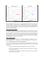
Surface Chloride Build Up
The model determines a maximum surface chloride concentration, Cs, and the time taken
to reach that maximum, tmax, based on the type of structure, its geographic location, and
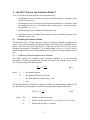
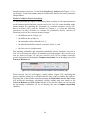
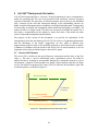
exposure, as input by the user. For example, if the user selects a bridge deck in an urban
area of Moline, Illinois, the model will use the surface concentration profile shown in the
left panel of Figure 2.1. Alternatively, the user can input his own profile, in terms of
maximum surface concentration and the time (in years) to reach that maximum. Life-365
v2.2 includes the additional ability to input a maximum surface concentration based on
ASTM C1556 data calculations.
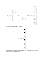
Figure 2.1. Examples of Concrete Surface History and Environmental
Temperatures
Temperature Profile
The model determines yearly temperature profiles based on the user’s input for
geographical location using a database compiled from meteorological data. For example,
if the user selects Moline, Illinois, the model will use the temperature profile in the right
panel in Figure 2.1. Alternatively the user can input temperature profile relevant to the
location, in terms of monthly average temperatures in either degrees Celsius (if the
project is using SI units) or degrees Fahrenheit (if the project is using US units).
Base Case Concrete Mixture
The base case concrete mixture assumed by the model is plain portland cement concrete
with no special corrosion protection strategy. For the base case, the following values are
assumed:
D28 =
1 x 10(-12.06 + 2.40w/cm) meters-squared per second (m2/s) ,
11
Eq. 4
m
=
Ct =
0.20, and
Eq. 5
0.05 percent (% wt. of concrete).
Eq. 6
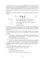
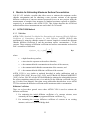
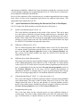
The relationship between D28 and the water-cementitious materials ratio (w/cm) is based
on a large database of bulk diffusion tests. The nature of the relationship is shown in
Figure 2.2 (corrected to 20°C). The value of m is based on data from the University of
Toronto and other published data and decreases the diffusion coefficient over the course
of 25 years, after which point Life-365 holds it constant at the 25-year value, to reflect
the assumption that hydration is complete. The value of Ct is commonly used for servicelife prediction purposes (and is close to a value of 0.40 percent chloride based on the
mass of cementitious materials for a typical concrete mixture used in reinforced concrete
structures).
Relationship Between D 28 and W/CM
2
Diffusion Coefficient, D 28 (m /s)
1E-10
1E-11
1E-12
0.3
0.4
0.5
0.6
W/CM
Figure 2.2. Relationship Between D 28 and
w/cm
It should be noted that these relationships pertain to concrete produced with aggregates of
normal density and may not be appropriate for lightweight concrete.
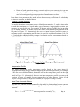
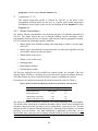
Effect of Silica Fume
The addition of silica fume is known to produce significant reductions in the permeability
and diffusivity of concrete. Life-365 applies a reduction factor to the value calculated for
portland cement, DPC, based on the level of silica fume (%SF) in the concrete. The
following relationship, which is again based on bulk diffusion data, is used:
DSF =
DPC ·e-0.165·SF.
Eq. 7
The relationship is only valid up to replacement levels of 15-percent silica fume. The
model will not compute diffusion values (or make service life predictions) for higher
levels of silica fume.
12
Effect of Silica Fume
1
2
DSF / DPC (m /s)
0.8
0.6
0.4
0.2
0
0
5
10
15
Silica Fume (%)
Figure 2.3. Effect of Silica Fume on D SF
Life-365 assumes that silica fume has no effect on either Ct or m.
Effect of Fly Ash and Slag
Neither fly ash nor slag are assumed to effect the early-age diffusion coefficient, D28, or
the chloride threshold, Ct. However, both materials impact the rate of reduction in
diffusivity and hence the value of m. The following equation is used to modify m based
on the level of fly ash (%FA) or slag (%SG) in the mixture:
m
=
0.2 + 0.4(%FA/50 + %SG/70) .
Eq. 8
The relationship is only valid up to replacement levels of 50 percent fly ash or 70 percent
slag and m itself cannot exceed 0.60 (which would occur if fly ash and slag were used at
these maximum levels), that is, m must satisfy m ≤ 0.60. Life-365 will not compute
diffusion values (or make service life predictions) for higher levels of these materials, and
after 25 years holds the diffusion constant at the 25-year value to reflect that hydration is
complete.
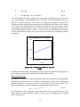
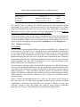
Figure 2.4 shows the effect of m for three mixtures with w/cm = 0.40 and with plain
portland cement (PC), 30 percent slag, and 40 percent fly ash. Table 1 lists these mixture
proportions and their computed the diffusion coefficients, for 28 days, 10 years, and 25
years. For years greater than 25, Life-365 uses the computed 25-year diffusion
coefficient.
13
Figure 2.4. Effects of Fly Ash and Slag on D t
Table 1. Effects of Slag and Fly Ash on Diffusion Coefficients
m
D28
D10y
D25y
-13
2
-13
2
-13
2
(<=0.60) (x 10 m /s) (x 10 m /s) (x 10 m /s)
PC
0.20
79
30
25
30 percent SG
0.37
79
13
9.3
40 percent FA
0.52
79
6.3
3.9
Effect of Corrosion Inhibitors
The model accounts for two chemical corrosion inhibitors with documented performance:
calcium nitrite inhibitor (CNI) and Rheocrete 222+ (a proprietary product from Master
Builders; in the Life-365 software, it is referred to as “A&E,” for “amines and esters”). It
is intended that other types of inhibitors can be included in the model when appropriate
documentation of their performance becomes available.
Ten dosage levels of 30 percent solution calcium nitrite are permitted in Life-365. The
inclusion of CNI is assumed to have no effect on the diffusion coefficient, D28, or the
diffusion decay coefficient, m. The effect of CNI on the chloride threshold, Ct, varies
with dose as shown in the following table.
14
Table 2. Effects of CNI on Threshold
CNI Dose
litres/m
3
Threshold, Ct
(% wt. conc.)
gal/cy
0
0
0.05
10
2
0.15
15
3
0.24
20
4
0.32
25
5
0.37
30
6
0.40
In addition, a single dose of Rheocrete 222+ (or amines and esters, as it is referred to in
the software) is permitted in the model; the dose is 5 litres/m3 concrete. This dose of the
admixture is assumed to modify the corrosion threshold to Ct = 0.12 percent (by mass of
concrete). Furthermore, it is also assumed that the initial diffusion coefficient is reduced to
90 percent of the value predicted for the concrete without the admixture and that the rate
of chloride build up at the surface is decreased by half (in other words it takes twice as
long for Cs to reach its maximum value). These modifications are made to take account of
the pore modifications induced by Rheocrete 222+ (or amines and esters), which tend to
reduce capillary effects (i.e. sorptivity) and diffusivity.
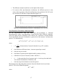
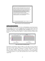
Effect of Membranes and Sealers
Membranes and sealers are dealt with in a simplified manner: Life-365 assumes that both
membranes and sealers only impact the rate of chloride build-up, and can only be
reapplied up to the time of the first repair. Membranes start with an efficiency of 100
percent, which deteriorates over the lifetime of the membrane; a lifetime of 20 years; and
no re-applications. This means that the rate of build-up starts at zero and increases linearly
to the same rate as that for an unprotected concrete at 20 years. As shown in the left panel
of Figure 2.5, surface chlorides for unprotected concrete (labeled “PC”) increases at a rate
of 0.04 percent per annum and reaches a maximum concentration of 0.60 percent at 15
years. In the right panel, surface chlorides for concrete protected by a default membrane
increase at a lower rate, but then reach the same rate after 20 years. The user can also set
his own values for initial efficiency, lifetime of the membrane, and re-applications.
15
Figure 2.5. Effects of Membranes and Sealers
Sealers are dealt with in the same way, except that the default lifetime is only 5 years. The
example in Figure 2.5 shows the effect of reapplying the sealer every 5 years. Each time
the sealer is applied, the build-up rate is reset to zero and then allowed to build up back to
the unprotected rate (0.04 percent per annum in the example) at the selected lifetime of the
sealer (5 years in the example).
Effect of Epoxy-Coated Steel
The presence of epoxy-coated steel does not affect the rate of chloride ingress in concrete,
nor would it be expected to impact the chloride threshold of the steel at areas where the
steel is unprotected. Consequently, the use of epoxy-coated steel does not influence the
initiation period, ti. However, it is assumed in the model that the rate of damage build up is
lower when epoxy-coated steel is present and these effects are dealt with by increasing the
propagation period, tp, from 6 years to 20 years.
Effect of Stainless Steel
In the current version of Life-365 it is assumed that grade 316 stainless steel has a
corrosion threshold of Ct = 0.50 percent (i.e., ten times the black steel Ct of 0.05 percent).
2.1.3
Initiation-Period Fickian Solution Procedures
The Life-365 Computer Program uses a finite-difference implementation of Fick’s second
law, the general advection-dispersion equation. Implicit in the model are the following
assumptions:
•
The material under consideration is homogeneous (e.g. no surface effects);
•
The surface concentration of chlorides around the concrete member is constant,
for any given point in time;
•
The properties of the elements are constant during each time step, calculated at
the start of each time step; and
16
•
The diffusion constant is uniform over the depth of the element.
•
For concrete slabs (one-dimension calculations), the diffusion process is only
active in the top portion of the slab and therefore only modeled in Life-365 in the
top 10 inches of a slab that is deeper than that (Figure 2.6).
Figure 2.6. Limited Modeling of Diffusion in Slabs Deeper than 10 Inches
One-Dimension Calculations (Walls and Slabs)
For the one-dimensional slabs and walls, the time-to-initiation is estimated
deterministically using a one-dimensional Crank-Nicolson finite difference approach,
where the future levels of chlorides in the concrete are a function of current chloride
levels. Specifically, the level of chloride at a given slice of the concrete i and next time
period t+1 is determined by
t +1
t +1
t
t
−rui+1
+ (1+ 2r)uit +1 − rui−1
= rui+1
+ (1− 2r) ruit + rui−1
,
where
(dt)
is dimensionless Courant–Friedrichs–Lewy (CFL) number,
2(dx)2
r
t
= d
€
dt
= the diffusion coefficient at time t, in meters-squared per second,
dt
= the time step, in seconds,
dx = the distance increment (total depth divided by number of slices),
uit = chloride level (%wt of concrete) at time t and slice i ,
€
i
= 1,…, I is the particular slice of concrete (and i = 0 is the top slice that holds
the external concentration of chlorides), and
t
= the time step in the initiation-to-corrosion period.
Rearranging terms and putting them in matrix form, the chloride levels at each time
period t+1 are solved from the equation
AU t +1 = BU t ,
where
€
17
"
$
$
A = {ait+1 } = $
$
$
$#
1
0
0
0
0 %
'
−r 1+ 2r −r
0
0 '
...
...
...
...
... ' ,
0
0
−r 1+ 2r −r '
'
0
0
0
0
1 '&
"u1t +1%
$ '
$ ... '
t +1
t +1
U = {ui } = $uit +1'
$ '
$ ... '
$#uIt +1'&
,
€
"
$
$
B = {bit+1 } = $
$
$
$#
1
0
0
0
0 %
'
r 1− 2r r
0
0 '
...
...
...
...
... ' , and
0
0
r 1− 2r r '
'
0
0
0
0
1 '&
"u1t %
$ '
$ ...'
t
t
U = {ui } = $uit '
$ '
$ ...'
$#uIt '&
The individual ui,t+1j are then be solved by rearranging terms:
U t +1 = A−1BU t .
€
The number r is required to be small for numerical accuracy.
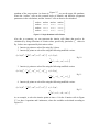
Two-Dimension Calculations (Square and Round Columns)
€
For two-dimensional columns, the time-to-initiation ideally can be estimated using a twodimensional Crank-Nicolson equation:
(1+ 2r)ui,t+1j −
r t+1
t+1
t+1
t+1
ui−1, j + ui+1,
= (1− 2r)ui,t j
(
j + ui, j−1 + ui, j+1 )
2
r t
t
t
t
+ (ui−1,
j + ui+1, j + ui, j−1 + ui, j+1 )
2
Eq. 9
where each term is defined as in the one-dimensional case above, but where each {i, j}
term is a square from the ith row and jth column of a square matrix of terms. Since the
chloride surface concentrations and interior steel locations are symmetric to the vertical
and horizontal centerlines of the column cross-section, we can solve using just one
18
quadrant of the cross-section. As shown in Figure 2.7, we use the upper left quadrant,
where the “surface” cells are the external levels of chloride, and therefore exogenous
parameters in the calculations, and the “interior” cells are those to be calculated.
!
#
#
#
#
"
surface surface surface surface $
&
surface interior (a) interior (a) interior (b) &
surface interior (a) interior (a) interior (b) &
&
surface interior (c) interior (c) interior (d) %
Figure 2.7. Single Quadrant in 2D Column
Also due to symmetry, we can represent the interior cells (those that need to be
calculated) by using reflections of certain values; specifically, particular ui,t+1j values in
Eq. 9 above are represented by their mirror value.
1. Interior (a) points are solved for using Eq. 9 above.
2. Interior (b) points are solved for using the following modified version:
(1+ 2r)ui,t+1j −
r t+1
(ui−1, j + ui+1,t+1 j + ui,t+1j−1 + ui,t+1j−1 ) = (1− 2r)ui,t j
2
r t
t
t
t
+ (ui−1,
j + ui+1, j + ui, j−1 + ui, j−1 )
2
Eq. 10
3. Interior (c) points are solved for using the following modified version:
(1+ 2r)ui,t+1j −
r t+1
(ui−1, j + ui−1,t+1 j + ui,t+1j−1 + ui,t+1j+1 ) = (1− 2r)ui,t j
2
r t
t
t
t
+ (ui−1,
j + ui−1, j + ui, j−1 + ui, j+1 )
2
Eq. 11
4. Interior (d) points are solved for using the following modified version:
(1+ 2r)ui,t+1j −
r t+1
t+1
t+1
t+1
ui−1, j + ui−1,
= (1− 2r)ui,t j
(
j + ui, j−1 + ui, j−1 )
2
r t
t
t
t
+ (ui−1,
j + ui−1, j + ui, j−1 + ui, j−1 )
2
Eq. 12
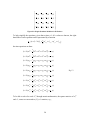
As an example, to solve the interior points at time t+1 for the 9 interior cells in Figure
2.7, we have 9 equations and 9 unknowns, where the variables are declared according to
Figure 2.8.
19
!
#
#
#
#
#
#
#
#
#"
u
0, 0
u
u
0,1 0, 2
u
1, 0
u
1,1
u
2, 0
u
u
2,1 2, 2
u
3, 0
u
3,1
u
1, 2
u
3, 2
$
u
0, 3 &
&
&
u
1, 3 &
&
u
2, 3 &&
&
u
3, 3 &%
Figure 2.8. Single Quadrant Variables in 2D Column
To help simplify the equations, given that at time t+1 all t values are known, the righthand side of each equation can be represented by a function
ui, j (t) = (1− 2r)ui,t j +
r t
t
t
t
ui−1, j + ui+1,
(
j + ui, j−1 + ui, j+1 ) ,
2
the nine equations are then:
r t+1 t+1 t+1 t+1
(u0,1 + u2,1 + u1,0 + u1,2 ) = u1,1 (t)
2
r t+1 t+1 t+1 t+1
t+1
(1+ 2r)u1,2
− (u0,2
+ u2,2 + u1,1 + u1,3 ) = u1,2 (t)
2
r t+1 t+1 t+1 t+1
t+1
(1+ 2r)u1,3
− (u0,3
+ u2,3 + u1,2 + u1,2 ) = u1,3 (t)
2
r t+1 t+1 t+1 t+1
t+1
(1+ 2r)u2,1
− (u1,1
+ u3,1 + u2,0 + u2,2 ) = u2,1 (t)
2
r t+1 t+1 t+1 t+1
t+1
(1+ 2r)u2,2
− (u1,1
+ u3,1 + u2,1 + u2,3 ) = u2,2 (t)
2
r t+1 t+1 t+1 t+1
t+1
(1+ 2r)u2,3
− (u1,1
+ u3,1 + u2,2 + u2,2 ) = u2,3 (t)
2
r t+1 t+1 t+1 t+1
t+1
(1+ 2r)u3,1
− (u2,1
+ u2,1 + u3,0 + u3,2 ) = u3,1 (t)
2
r t+1 t+1 t+1 t+1
t+1
(1+ 2r)u3,2
− (u2,2
+ u2,2 + u3,1 + u3,3 ) = u3,2 (t)
2
r t+1 t+1 t+1 t+1
t+1
(1+ 2r)u3,3
− (u2,3
+ u2,3 + u3,2 + u3,2 ) = u3,3 (t)
2
t+1
(1+ 2r)u1,1
−
Eq. 13
t +1
t +1
To be able to solve for each ui, j through matrix mathematics, the square matrices of ui, j
t
and ui, j terms are converted to (i*j) × 1 matrices, e.g.,
€
€
€
20
" t+1
t+1
$ u0,0 u0,1 ...
$ ut+1 ut+1 ...
1,1
$ 1,0
$ ...
... ...
$
t+1
t+1
U = {ui, j } =
ui,t+1j
$
$
...
...
...
$
t+1
t+1
... uI−1,J−1 uI−1,J
$
$
t+1
t+1
... uI,J−1
uI,J
$#
"
t+1
$ u0,0
$ ut+1
0,1
$
$ ...
%
$ ut+1
'
$ 1,0
'
$ ut+1
'
$ 1,1
'
$ ...
' ⇒ U t+1 = ut+1 = $ ut+1
{ k } $ i, j
'
'
$ ...
'
$ t+1
'
$ uI−1,J−1
'
$ ut+1
'&
$ I−1,J
$ ...
$ t+1
$ uI,J−1
$ ut+1
I,J
#
%
'
'
'
'
'
'
'
'
'
'
'.
'
'
'
'
'
'
'
'
'
&
For the 9x9 example, then, the U˙ t +1 vector is
"u0,0 %
$ '
$ u0,1 '
$u0,2 '
$ '
$u0,3 '
$ u1,0 '
$ '
$ u1,1 '
$ u1,2 '
$u '
1,3
t +1
t +1
˙
U = {uk } = $ '
$u2,0 '
$u '
$ 2,1 '
$u2,2 '
$u '
$ 2,3 '
$u3,0 '
$u '
$ 3,1 '
$u3,2 '
$u '
# 3,3 &
€
and the equations in Eq. 13 can be represented by AU˙ . The chloride levels at each time
period t+1 are solved from the equation
€
AU˙ t +1 = BU˙ t ,
t +1
€
€
21
or
U˙ t +1 = A −1BU˙ t .
Eq. 14
Inverting matrix A, however, is computationally expensive; computing initiation periods
could take from 1 to 15 minutes (or longer) per alternative. To overcome this time
expense, Life-365 €
uses a successive relaxation technique (SOC).
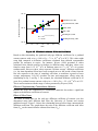
Validation of Initiation Period Estimates
Significant work has been conducted to compare the estimates of initiation period
calculated by Life-365 v2.2 against those of other models. With regard to 1-D (slab and
wall) estimates, the Life-365 v2.2 estimates have been compared to both Fick’s second
law Error Function Solutions as well as Life-365 v1.1 estimates. With regard to 2-D
square and round columns, the Life-365 v2.2 estimates have been compared to Life-365
v1.1 estimates.
For the 1-D case in particular, work has been conducted to compare the Life-365 v2.2
estimates (and indirectly the Life-365 v1.1 estimates) of initiation period to Fick’s second
law error function solution,
(
" x %+
c(x, t) = cs *1− erf $
'- ,
# 4Dt &,
)
Eq. 15
(where c(x,t) is the concentration at depth x and time t, c s is the surface concentration, erf
is the error function, and D is the diffusion coefficient), which for particular settings are
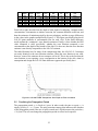
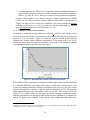
theoretically equivalent.1 Tests of estimates by the two methods show a good ‘fit’ of the
two concentration values shown in Figure 2.9.€2
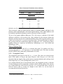
Table 3. Life-365 v2.2 and ERF Comparison
#
0
1
2
3
4
5
6
7
8
9
10
11
12
Slab
Depth
(mm)
200.0
200.0
200.0
200.0
200.0
200.0
200.0
200.0
200.0
200.0
200.0
200.0
200.0
Rebar
Depth
(mm)
10.0
20.0
30.0
40.0
50.0
60.0
70.0
80.0
90.0
100.0
110.0
120.0
130.0
Surface
Conc.
(%wt)
1.000
1.000
1.000
1.000
1.000
1.000
1.000
1.000
1.000
1.000
1.000
1.000
1.000
Init
Conc
(%wt)
0.050
0.050
0.050
0.050
0.050
0.050
0.050
0.050
0.050
0.050
0.050
0.050
0.050
D28
(m*m/s)
8.870E-12
8.870E-12
8.870E-12
8.870E-12
8.870E-12
8.870E-12
8.870E-12
8.870E-12
8.870E-12
8.870E-12
8.870E-12
8.870E-12
8.870E-12
L365
Init
(yrs)
0.1
0.2
0.5
0.8
1.2
1.8
2.3
3.1
3.8
4.8
5.8
6.8
8.0
ERF
Init
(yrs)
0.1
0.2
0.5
0.8
1.2
1.8
2.3
3.1
3.8
4.8
5.8
6.8
8.0
Avg.
Diff
(%wt)
0.02641412
0.00321595
0.00143871
0.00137160
0.00138123
0.00139729
0.00140854
0.00148045
0.00146977
0.00150216
0.00152166
0.00154075
0.00161298
1
The Crank Nicolson finite difference approach used in Life-365 v2.2 1-D slab and wall calculation is an
approximation to the Fick’s Second Law solution and thus an approximation to the error function direct
solution. To make the comparison, a particular set of Life-365 v2.2 parameters must be held constant,
including the surface concentration over time, the diffusion coefficient over time, and the external
temperature over time.
2
The values shown may not exactly match the current version of Life-365, due to continual refinements
being made to the codebase.
22
#
13
14
15
16
17
18
Slab
Depth
(mm)
200.0
200.0
200.0
200.0
200.0
200.0
Rebar
Depth
(mm)
140.0
150.0
160.0
170.0
180.0
190.0
Surface
Conc.
(%wt)
1.000
1.000
1.000
1.000
1.000
1.000
Init
Conc
(%wt)
0.050
0.050
0.050
0.050
0.050
0.050
D28
(m*m/s)
8.870E-12
8.870E-12
8.870E-12
8.870E-12
8.870E-12
8.870E-12
L365
Init
(yrs)
9.3
10.8
12.7
15.5
22.2
500.0
ERF
Init
(yrs)
9.2
10.7
12.1
13.7
15.3
17.1
Avg.
Diff
(%wt)
0.00198084
0.00325238
0.00693507
0.01761402
0.05659158
0.68549250
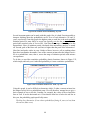
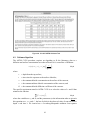
From left to right, the table lists the depth of slab, depth of reinforcing, constant surface
concentration, concentration to initiate corrosion, the constant diffusion coefficient, and
then the estimates of initiation period by the two techniques, and the average differences
in the values in the graphs exemplified by Figure 2.9. This figure specifically plots the 60
Life-365 point estimates of concentration (one for each ‘slice’ in the finite difference
mesh) against the ‘continuous’ error function estimates. Finally, it lists whether the ERF
value computed is valid, specifically, whether the error function computed a zero
concentration at the depth of the bottom of the slab. If it does not, then the error function
estimate is not directly comparable to the Life-365 estimate.
The table illustrates how for many of the comparisons done, the Life-365 v2.2 estimates
are nearly identical to the error function estimates. When the error function is not valid,
however, some of the estimates do not compare well at all. This is due to the fact that the
error function is not reporting a zero concentration at the bottom of the slab, when by
assumption and design the Life-365 finite difference approach specifically does.
Figure 2.9. Life-365™/ERF Comparison: Over Depth at Time of Initiation
2.2
Predicting the Propagation Period
The propagation period, tp, is fixed at 6 years. In other words, the time to repair, tr, is
simply given by tr = ti + 6 years. The only protection strategy that influences the duration
of the propagation period is the use of epoxy-coated steel, which increases the period to tp
= 20 years. The user can change the propagation period to reflect local expertise.
23
2.3
Repair Schedule
The time to the first repair, tr, is predicted by Life-365 from a consideration of the
properties of the concrete, the corrosion protection strategy, and the environmental
exposure. The user needs to estimate the cost and extent of this first repair (i.e., the
percentage of area to be repaired) and the fixed interval over which future repairs are
conducted.
2.4
Probabilistic Predictions of Initiation Period
Life-365 includes probabilistic predictions of the initiation period, based on Bentz
(2003). These predictions are calculated using the following steps:
a) Estimate time to first corrosion for the “best guess” or average values of the
inputs, that is, the values input by the user.
b) For each of five specific input variables (D , Cs, m, C , x ), estimate five additional
time to first corrosions, where each is individually adjusted by 10 percent.
28
t
d
c) Use the results of steps b) and step a) to estimate the derivative of corrosion
initiation time with respect to each of the five variables. This determines the
sensitivity of initiation period to variations in each of the input variables.
d) Use the results from step c) to estimate a single parameter of variability, similar to
a standard deviation, for a log-normal assumed variation of time to corrosion
initiation (shown by Bentz to work well), where the average value of this
distribution is taken from the deterministic analysis in step a) and the variability
of this assumed distribution is determined from the results of steps b) and c).
2.5
Estimating Life-Cycle Cost
To estimate life-cycle cost, Life-365 follows the guidance and terminology in ASTM E917 Standard Practice for Estimating the Life-Cycle Cost of Building Systems. This
includes the process of
1. Defining a base year, study period, rates of inflation and discount, project
requirements, and alternatives that meet project requirements;
2. Calculating the present value of future costs;
3. Reporting results in present value (constant dollar) and current dollar terms; and
4. Conducting uncertainty and sensitivity analysis.
User Input Parameters
The user is responsible for providing the following cost information needed for the lifecycle cost analysis:
•
Cost of concrete mixtures (including corrosion inhibitors) for the various
corrosion protection strategies under consideration,
•
Cost, coverage (percent of surface area), and timing of repairs,
•
Inflation rate, i, and
•
Real discount rate, r.
Life-365 provides the following default costs for the included rebars:
24
•
Black steel = $1.00/kg ($0.45/lb)
•
Epoxy-coated rebar = $1.33/kg ($0.60/lb)
•
Stainless steel = $6.60/kg ($2.99/lb)
The user should review and if necessary change the costs of these materials to better
reflect actual project costs in his area.
2.6
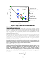
Calculating Life-Cycle Cost and Current Costs
2.6.1 Life-Cycle Cost (Present Worth) Calculations
Life-cycle cost is calculated as the discounted present value of the initial construction
costs and the repair costs over the life of the structure (Figure 2.10). Life-cycle cost is
expressed in either total dollars or dollars per unit area of the structure (e.g. dollars per
square meter).
Figure 2.10. Construction and Repair Costs over the Life of the Structure
The initial construction costs are calculated as the sum of concrete costs, steel (or other
reinforcement) costs, and any surface protection (membrane or sealer) costs. The present
worth of all costs are specifically calculated as follows. First, Life-365 costs are inputted
in terms of what they cost today, specifically, what they cost in the first year of the study
period. To compute a cost’s discounted present value, then, it must first be inflated to the
future using an annual rate of inflation. (These inflated costs are the current costs listed I
the Life-365 life-cycle cost results.) Each future, inflated cost is then discounted to the
present value (first year) using the nominal discount rate (n), which represents the
combined effects of inflation and the real discount rate (d), the latter of which represents
the time value of money. The nominal discount is defined as the product of the annual
inflation rate (reflecting changes in the prices) and annual real discount rate (reflecting
the time value of money):
(1 + n) = (1 + i)(1 + d ).
Eq. 16
Mathematically, given a cost 𝑐!! which occurs at time t but is expressed in terms of prices
at time 0, and inflation rate i, the current cost of that cost when it occurs is computed as
current cost (c 0t ) = c 0t (1 + i) t ,
Eq. 17
and the present value or constant cost of cost c in year t is calculated as
c 0t
(1 + i) t
present value = constant cost (c ) = c
=
(1 + n) t (1 + d ) t
t
0
t
0
25
.
Eq. 18
3 Life-365™ Computer Program Users Manual
The concrete service life and life-cycle costing methodologies described in Chapter 2 are
implemented in the Life-365 Computer Program in a way that allows for easy input of
the project, structure, environmental, concrete, and economic parameters, and for rapid
sensitivity analysis of the parameters that most influence concrete service life and lifecycle cost. This chapter describes how to install, start, and use the Life-365 Computer
Program, and then describes additional optional features designed for experienced
practitioners.
3.1 Installing Life-365
Life-365 runs on personal computers that can run Java, including those running Microsoft
Windows or Apple OS X. It requires Java 1.7 or higher (also known as “Java 7.0 or
higher”). Mac OS X now strongly prefers Java 1.7, which can be installed from the Java
website. Windows Java 1.6 and higher is produced by Oracle, and can be installed by
accessing http://java.sun.com and then selecting the appropriate web page for installing
the most recent version of the Java Runtime Environment [JRE].
To install Life-365 from either a CD or the Life-365 website (http://www.life-365.org):
•
On Windows computers:
o Uninstall any previous versions of Life-365 v2.0 or higher that are
installed on the computer, by going to the Windows Control Panel,
accessing the “Add or Remove Programs” application, and removing these
versions of Life-365.
o Once removed, access the new version of Life-365 and then double-click
your mouse on the Windows install file; this will run through a quick
installation program that, among other things, puts a program-start icon in
your Programs folder.
•
On Apple OS X computers:
o Double-click your mouse on the Apple install file; this will mount a disk
drive on your desktop. Open the disk drive and drag the Life-365 program
into your Applications Folder.
o Different versions of Life-365 can run simultaneously on Mac OS X,
although we recommend using only the most recent version.
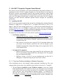
3.1.1 If You Have Problems Installing on Windows Computers:
If the installation process exits abruptly without apparently installing any files, your
computer likely does not have Java installed or does not have at least Java 1.7 installed.
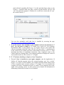
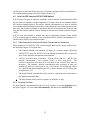
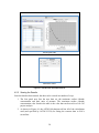
1. To see if Java is installed on your Windows computer, access the Control
Panel and then double-click on the Java icon (if you do not have a Java icon in the
Control Panel, then you very likely do not have Java installed). In the panel that
opens, select the “Java” tab and then the “Runtime settings...” or similar tab. On
this panel there should be a list of Java versions installed; check to see that Java
1.7 or higher is installed and enabled. Depending on the version of Windows, the
26
panel will look something like Figure 3.1; in this particular figure, there is only
version 1.7 installed; make sure other versions are not checked. Life-365 will
“ask” this particular computer’s Windows for a sufficient version and will “get”
the version it needs, 1.7.
Figure 3.1. Windows Java Settings Panel
You can also optionally verify that Java is installed by accessing the page
http://www.java.com/en/download/installed.jsp.
2. If you do not have Java installed or your installed version is less than Java 1.7
(6.0), you will need to install it. To install Java, search for “Java Runtime
Environment (JRE)” on the Internet (e.g., via Google) and go to the website that
offers the download of this JRE. Since Life-365 will run on Java 1.7, install the most
recent version of Java (which at the time of this manual’s release is Java 1.7). Then
download and follow its installation instructions. Once completed, return to the
Control Panel Java Settings Panel. Your computer should now display the version of
Java installed; make sure this version is 1.7 or higher.
3.1.2 If Problems Installing on Apple or Linux Computers:
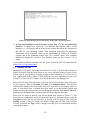
1. To see if Java is installed on your Apple computer, start the Applications à
Utilities à Terminal program and at the command prompt, type “java -version”
(Figure 3.2). If Java is in fact installed, your computer will then return which version
of Java is installed; make sure this version is 1.7 or higher. If it is not installed, the
computer will return “command not found” or similar. If your computer runs a nonApple, Unix operating system, see that system’s users manual for information for
determining if and which version of Java is installed.
27
Figure 3.2. Determining Current Java Version in Mac OS X Terminal Console
2. If Java is not installed or you do not have at least Java 1.7 (7.0), you will need to
install it. To install Java, search for “Java Runtime Environment (JRE)” on the
Internet (e.g., via Google) and go to the Oracle website that offers the download of
this JRE for your operating system. Then download and follow its installation
instructions. Once completed, return to the Applications à Utilities à Terminal
program and at the command prompt type “java -version” again. Your computer
should now display the version of Java installed; make sure this version is 1.6 or
higher.
If you still have problems installing Life-365, please contact the Life-365 Consortium III,
at http://life-365.org/contact.html.
3.2 Starting Life-365
Installing Life-365 puts a start menu item labeled “Life-365” in your Windows Programs
folder (accessible from the Start button in the lower left-hand corner of your screen)
and an icon on your desktop; on Apple computers there should be a Life-365 icon in
your Applications folder. (Other, UNIX platforms may not, depending on your Java
settings). To start Life-365, simply select this menu item or the desktop icon.
When Life-365 starts for the first time, it will ask you to select the base units of measure
for your projects, either in SI metric, US units, or Centimeter metric. This selection
will determine whether all of your inputs need to be expressed in, for example, meters or
yards. If you decide later to change these base units, go to the Default Settings and
Parameters tab at the bottom of the screen, change the selection in the Base Units field,
and then press the Save button; all future projects will use this new base unit.
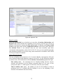
When Life-365 starts in general, your screen should look similar to Figure 3.3. This
screen has two components: on the left-hand side there is a navigation menu, under the
Navigator section, that lets you open new or existing Life-365 project files; under the
Settings section, it lets you change the default settings and get help with particular
screens; and under the Tips section, it displays text that gives you information and tips
on using the software.
28
Figure 3.3. Startup Screen
There are also three tabs at the bottom of the screen:
1. The Current Analysis tab, which contains the current project on which you
are working (on startup, this tab shows the opening banner in Figure 3.3);
2. The Default Settings and Parameters tab, which allows you to set the
default values of parameters to be used in all projects (see Section 3.9.1, p. 34);
and
3. The Online Help tab, which offers detailed explanations of the key windows
and features in the Life-365 Computer Program.
To start a new project, select Open new project from the left-hand-side navigation
menu; a complete project will be created for you, with two alternatives, each of
which has a baseline concrete mixture. To open a previously created and saved project,
select Open existing project…
When a new or existing project is opened, the main panel will show seven tabs at the
top. To conduct an analysis, each tab can and should be accessed from left-most tab,
Project, to right-most tab, LCC Report. Additionally, the left-hand Navigator pane has a
list of chronological Steps that divides your Life-365 analysis into logical analytical
components:
1. Define project: e.g., input the title, description, structure type, units of measure,
and economic values.
2. Define alternatives: e.g., input the titles and descriptions of the alternatives that
meet the project requirements.
29
3. Define exposure: input the location and type of structure (so as to set the
chloride and temperature exposure conditions).
4. Define mix designs: input the concrete mixture and corrosion protection strategy
for each alternative.
5. Compute service life: calculate the service life of each alternative.
6. Define project costs: input the initial construction, barrier, and repair costs and
repair schedule.
7. Compute life-cycle cost: calculate and sum the present value of all costs, for
each alternative, and compare.
Each of the software tabs that execute these steps is discussed in turn.
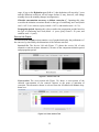
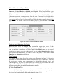
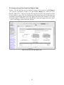
3.3
Project Tab
The Project tab allows you to complete Steps 1 and 2 above, specifically, to name the
project and set the type and dimensions of the structure, the economic analysis
parameters, and the number and names of the alternative projects (Figure 3.4).
Figure 3.4. Project Tab
Identify Project
In this section you can set the project Title, Description, Analyst, and Date, most of
which are used to simply document the project, but also are part of the report displayed in
and printed from the LCC Report tab (Figure 3.17).
Select Structure Type and Dimensions
In this section you set a number of fundamental parameters about the structure itself. Use
the Type of structure drop-down box to select the structure, which also sets the means of
chloride ingress, e.g., 1-D (one dimensional). Use the Thickness (for 1-D structures) or
30
Width (for 2-D structures), and Area or Total Length fields to set the total volume of
concrete, which is used to calculate total concrete installation costs, and to set the
surface area of the concrete structure, which is used to calculate repair costs. Use the
Reinf. depth field to set the distance over which chlorides travel from surface to the
steel reinforcement. Finally, use the Chloride concentration units drop-down box to
select the units of measure of the chloride exposure and concrete materials; if you select
SI metric or Centimeter metric as your Base unit, then your Concentration units
options are % wt. conc. and kg/cub. m.; if you select US units, then your options are %
wt. conc. and lb/cub yd.
Define Economic Parameters
Four parameters are used to set the period and interest rates over which life-cycle cost is
computed. Set the Base year to be the current year or other initial year that is relevant
to your analysis. Set the Analysis period to be the period of time over which lifecycle cost should be calculated; 75 years is a common period and Life-365 allows the
user to select up to 200 years.
The Inflation rate (%) is the annual rate at which the prices of goods and services will
increase over the future; the Real discount rate (%) is the annual rate at which future
costs are discounted to base-year dollars, net of the rate of inflation (that is, it is the real
discount rate, which does not include the effects of changes in the prices of goods and
services). Federal infrastructure projects use a discount rate published in OMB
Circular No. A-94. Life-365 comes with the most recent figures of inflation and discount
rate, as suggested by the OMB Circular and as published in Energy Price Indices and
Discount Factors for Life-Cycle Cost Analysis (2006).3
At the time of this publication, the suggested long-run real discount rate was 2.0 percent
and the long-run general inflation was calculated to be 1.8 percent (based on the long-run
nominal discount rate of 3.8 percent and Eq. 16 (p. 25). Private sector projects, however,
can use their own rates of inflation and real discount.
Define Alternatives
Use this section to set the number, names, and descriptions of alternatives to be analyzed
and compared. Use the Add a new alt and Delete currently selected alt buttons to
create and delete alternatives, respectively, and double-click the mouse on the
alternative’s Name or Description fields to change them.
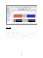
3.4
Exposure Tab
The Exposure tab (Figure 3.5) is used to set the exposure of the concrete to
external chlorides, and to set the monthly temperatures to which the concrete is exposed.
3
See: Rushing, Amy S., and Fuller, Sieglinde K., Energy Price Indices and Discount Factors for Life-Cycle
Cost Analysis, NISTIR 85-3273-18. Gaithersburg, MD: National Institute of Standards and Technology,
November 2012.
31
Figure 3.5. Exposure Tab
Select Location
When the Use defaults box is checked, you can select a Location, Sub-location, and
Exposure that closely matches the conditions of your project, and Life-365 will use its
database of locations to estimate the Max surface conc. of chlorides and Time to build
to max in the upper panel and the Temperature History in the lower panel. When the
Use defaults button is not checked, then the user must manually input these
concentration and temperature values. In Life-365 v2.2, the user can manually input their
own maximum chloride level by also using values measured in accordance with ASTM
C1556 (see Section 4 for details).
Define Chloride Exposure
The rate of buildup and maximum level of external chloride concentrations affect the
rate of chloride ingress and ultimately concrete service life. Use the following variables
to set these rates, and confirm them with the Surface Concentration graph on the right.
Max surface conc. – the maximum level of chloride buildup that the concrete
structure will experience over its lifetime, measured either in % wt. conc. or base
unit-specific units, i.e., either kg/cub. m. (SI metric) or lb/cub yd (US units).
Time to build to max (yrs) – the number of years for the buildup to reach its
maximum level. It is assumed that the buildup is zero at the beginning of the
structure’s life and that it increases linearly.
32
Define Temperature Cycle
When the Use defaults box is not checked, the user needs to input the annual temperature
cycle to which the project is exposed; these temperatures are part of the service life
calculations that determine the effects of temperature on concrete diffusivity. If the user
selected either SI metric or Centimeter metric as the Base unit in the Project tab, then
the temperatures must be input in degrees Celsius; if the user selected US units as the
base unit, then temperatures must be input in degrees Fahrenheit.
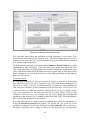
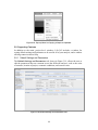
3.5
Concrete Mixtures Tab
The Concrete Mixtures tab (Figure 3.6) is used to define the concrete mixtures for
each project alternative defined in the Project tab.
Figure 3.6. Concrete Mixtures Tab
Define Concrete Mixtures
This section allows the user to input the concrete mixtures and corrosion protection
strategies of each alternative. Because the calculation of concrete service life is
computationally intensive, you need to press the Calculate service lives button after
inputting the mixtures and strategies to make the calculations.
Check-mark the Compute uncertainty box if you want Life-365 to compute
the uncertainty of service life for each concrete mixture. In general, this is a
calculation reserved for advanced users of Life-365; to understand Life-365
uncertainty analysis, press the Help button to the right, and see Section 3.10 (pg. 45) of
this manual for details on how to use service life uncertainty in your analysis. For
now, leave the Compute uncertainty unchecked.
33
Selected mixture
This section lists the properties of the concrete mixture selected in the upper, Define
Concrete Mixtures, panel, and allows you to edit these properties. To see the properties
of any one of your concrete mixtures, simply click the row of the mixture in this upper
panel.
Mixture group – use this section to set the water-cementitious materials ratio
(w/cm) of your concrete mixture, and whether and to what level you are using
SCMs (Slag, Class F fly ash, or Silica fume). Enter the SCM amounts in percent
substitution.
Rebar and Inhibitors groups – use these sections to select the type of reinforcing
steel used in your structure (Black steel, Epoxy coated, or 316 Stainless, which
affects the initiation period and propagation period of the concrete service life).
The Rebar % vol. concrete field is used to input the percent of the concrete that is
steel; this is used to calculate the cost of steel in your concrete structure, where the
costs of the steels are set in (1) the Individual Costs tab, under the Default
Concrete and Repair Costs tab), and (2) the Default Settings and Parameters
tab at the bottom of the Life-365 window. Use the Inhibitor drop-down to
include in your mixture any corrosion inhibitors that will be used. The units of
measure of these inhibitors are either l/cub. m. (liters per cubic meter) or gal/cub.
yd (gallons per cubic yard), depending on the Base unit selected in the Project tab.
Barriers group – use this section to include a membrane or sealant application on
the concrete. If the Use defaults box is checked, then you simply select
membrane or sealant; if not checked, then you must input the values of Initial
efficiency (%), Age at failure (yrs), and # times reapplied for the particular one
selected.
Custom Mixture Properties
In addition to inputting the constituent physical concrete mixture and other corrosion
protection strategies, Life-365 allows the user to input directly the model properties used
to calculate service life. (Doing so will potentially generate results that override one or
more of the basic Life-365 modeling assumptions, so check-marking the Custom button
the first time will cause a pop-up window to appear asking that the user confirm he is
aware of this.) The set of Custom input fields together override the model, in the
following ways.
Initial diffusion coefficient, D28. Inputting the initial diffusion coefficient directly
overrides the calculation of D28 based on w/cm ratio and the level of silica fume.
Diffusion decay index, m. Inputting this index directly overrides the calculation of
m based on the levels of slag and fly ash. The value of m, however must still be
between 0.2 and 0.6.
Hydration years. By default, Life-365 models hydration taking 25 years, where the
effects of hydration on concrete diffusivity are modeled by m; if under these default
settings the modeled concrete’s diffusivity continues to decline past 25 years, Life365 holds the concrete’s diffusion coefficient constant after 25 years. Inputting a
custom hydration value here changes the number of years after which hydration
34
stops; if you set the Hydration (yrs) field to 5, then hydration will stop after 5 years
and the diffusion coefficient will no longer decline (it may, however, still change
monthly due to the monthly changes in temperature).
Chloride concentration necessary to initiate corrosion, Ct. Inputting this value
overrides the initiation corrosions based on the type of reinforcing steel used (black
steel = 0.05 % wt. concrete, epoxy-coated = 0.05 %, and stainless steel = 0.5 %).
Propagation period. Inputting this value overrides the propagation periods based on
the type of reinforcing steel used (black = 6 years, epoxy-coated = 20 years, and
stainless steel = 6 years).
Service Life Graphs
The Service Life Graphs section contains a set of graphs that display the performance of
the concrete, by time and by the dimensions of the concrete structure.
Service Life. The Service Life tab (Figure 3.7) shows the service life of each
alternative concrete mixture alternative, in terms of the component initiation period
and propagation period.
Figure 3.7. Service Life Tab
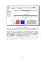
Cross-section. The cross-section tab (Figure 3.8) shows a cross-section of the
chloride concentration of the concrete mixture at the point of initiation of
corrosion. The alternative shown is selected from the left-hand-side Select: dropdown box.
Figure 3.8. Cross-section Tab
35
The chloride concentration scale on the left-hand side indicates the meaning of the
colors in the right hand graph. The top of the white rebar “holes” should have a
color that reflects the level of chloride concentration at initiation, which in this
graph is 0.05 % wt of concrete.
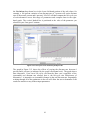
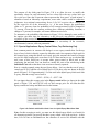
Initiation. This tab (Figure 3.9) shows two graphs: the concentration of chlorides
at the time of initiation, by depth of the structure (the left graph, Conc Versus
Depth); and the concentration of chlorides at the rebar depth, by point in time,
up to initiation (the right graph, Conc Versus Time at Depth). The left graph
includes a vertical dashed line indicating the depth of reinforcing, and the right
graph a dashed line indicating the year of initiation.
Figure 3.9. Concrete Initiation Graphs
The right graph shows that the Base case mixture hits initiation in 5 years at a rebar
chloride concentration of about 0.05 % weight of concrete, while the Alternative 1
mixture hits initiation in 17 years with a rebar concentration of 0.05 % weight of
concrete.
Concrete Characteristics. Finally, the Conc Characteristics tab (Figure 3.10)
displays two additional graphs that help interpret the performance of the concrete
mixtures. The left-hand-side graph, Diffusivity Versus Time, shows how the
calculated concrete chloride diffusivity changes over the initiation periods, by
mixture. The right-hand-side graph, Surface Concentration Versus Time,
shows how the concrete surface conditions change over the same period.
Figure 3.10. Concrete Characteristics Tab
36
For this particular graph, the left panel indicates that both mixtures have the same
chloride diffusivity characteristics (different mixtures could potentially have
very different characteristics and thus lines in this graph); the oscillations are
caused by the effect of annual temperature variation. The right-hand graph shows
that both mixtures have the same surface concentrations; this would not be true if
the mixtures had membrane or sealant applications.
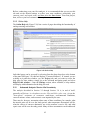
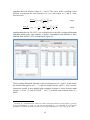
3.6 Individual Costs Tab
The Individual Costs tab (Figure 3.11) allows you to edit the different constituent cost
and cost parameters, and view the effects they have on the constituent costs that make up
life-cycle cost.
Figure 3.11. Individual Costs Tab
Set Concrete Costs
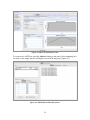
In the upper-left corner of the screen, the Set Concrete Costs tab allows the user to set
specific values for the concrete mixture costs. Initially, this table displays the default
concrete cost that is listed in Concrete & Steel section of the Default Settings and
Parameters tab (located at the bottom of the Life-365 screen); this default cost
should represent the cost of concrete only, without inhibitors, barriers, or steel (these costs
are all used later, when calculating the initial construction cost). If, however, a particular
mixture uses, for example, SCMs or other materials that cause concrete costs to be
different than the default cost, enter that cost in this table, by double-clicking on the cost
itself; doing so will cause the User? box to be check-marked. If you enter a cost and need
to return that cost to the default cost, simply uncheck the User? box.
37
Default Concrete and Repair Costs
This section (Figure 3.12) lists the costs associated with three categories of project costs:
Concrete & Steel, Barriers & Inhib., and Repairs. When you first start your
project, Life-365 uses the default values of these costs listed in the Default
Settings and Parameters tab (located at the bottom of the Life-365 screen).
(These are converted, when necessary, from the units of measure listed in this tab to
the units used in your project. If you save your project and access it later, it will list again
your project values of cost.) If you would like to make the values currently shown in this
project to be the default values for all future projects, press the Set as defaults
button.
Figure 3.12. Default Concrete and Repair Costs
Costs for Each Alternative Mix Design
Based on these costs, the Project Costs section lists up to three costs: (1) the
Construction cost, or cost of mixing/placing the concrete; (2) the Barrier cost, or the
cost of applying a membrane or sealer; and (3) the Repair cost, or the cost of
repairing the concrete over the study period. Use the Select Alternative drop-down
box to select which alternative you want to view in this panel, as well as in the Cost
Time-line for Alternative graph below.
Cost Timeline
This section shows a time-line of the project costs. The graph in Figure 3.11 shows in
particular the initial construction cost occurring between year 0 and year 1, and then
the repair costs starting after construction (as indicated by the red arrow) and
continuing every 10 years (as indicated by the vertical gray lines within the white
box) until year 75. Use the Select Alternative drop-down box above to see the
different cost timelines of your different alternative mixtures.
3.7 Life-Cycle Cost Tab
Once the project, exposure, concrete mixtures, and individual costs data have been
entered, the resulting life-cycle cost of the alternative mixtures are computed and can
be viewed and compared in the Life-cycle Cost tab (Figure 3.13).
38
Figure 3.13. Life-Cycle Cost Tab
Life-Cycle Cost
This first tab displays the life-cycle cost of each alternative, in tabular form, as a total
(the colored bars) and by component cost (the black and gray bars).
Timelines
The Timelines tab (Figure 3.14) shows the constituent costs over time. This tab will
initially show just one of the four timeline figures, but can show all four together when
the user checks the Show all four time series graphs together box. The upper two
panels show the individual-year and cumulative constant-dollar costs, that is, costs that
have been adjusted to account for the effects of increases in the prices of
materials and labor (the inflation rate) and time-value of money (the real discount
rate), and that are summed to compute life-cycle cost.
39
Figure 3.14. Life-Cycle Cost: Timelines Tab
The lower two panels show the individual-year and cumulative current-dollar costs,
which are the costs adjusted for inflation only. This current-dollar measure is not a
measure of life-cycle cost, but is a useful estimate of the actual dollars that are estimated
to be spent over the study period.
For these particular alternatives, the upper-right Cumulative Present Value gives a good
explanation of why Alternative 1 (the blue line in the graph) has lower life-cycle
cost: while it does have a slightly higher cost at initial construction and identical repair
costs, it has fewer repairs due to the longer service life (specifically, its first repair occurs
later), resulting in a total level in the last year of the study period that is lower than the
Base case (the red line).
Sensitivity analysis
An important component of life-cycle analysis is sensitivity analysis, or determining
how sensitive your results are to changes in any of the underlying assumptions or
inputs for economic, concrete, constituent-material, or repair costs. After making your
first, best-guess estimates of these parameters in the previous tabs, Life-365 gives you
at least two ways of conducting sensitivity analysis: the first way is to simply change
any of the parameters in the previous tabs and see what effects it has on each
alternative’s life-cycle cost. For example, you can easily change the environmental
conditions of the mixtures (e.g., switching location from New York, NY to Philadelphia,
PA) or some of the properties of your mixtures.
A second, efficient way to conduct sensitivity analysis on a subset of all parameters is
to use the Sensitivity Analysis tab (Figure 3.15). In this tab, you select one of the
predefined parameters listed in the left-hand tree (Discount rate (%) is selected in
the figure) and then select a range of values for this parameter by selecting from
40
the Variations drop-down box in the lower-left-hand portion of the tab (where, for
example, a 100 percent variation of an discount rate of 3 percent will create discount
rates of between 0 percent and 6 percent). Life-365 will then compute the life-cycle cost
of each alternative across this range of parameters and compare them in the righthand graph. The vertical dashed line is positioned at the value of the parameter you
selected as your “best guess” estimate.
Figure 3.15. Life-Cycle Cost: Sensitivity Analysis Tab
The graph in Figure 3.15 shows the effects of varying the discount rate between 0
percent and 6 percent (as indicated by the graph’s horizontal axis). The graph shows
that Alternative 1 has lower life-cycle cost than the Base case, regardless of the
(reasonable) real discount rate selected, that is, the life-cycle cost effectiveness of
Alternative 1 is insensitive to (reasonable) changes in the real discount rate. Sequentially
working through all of the parameters in the tree will allow the user to determine if the
results are sensitive to any of these input parameters.
41
3.8 Service Life and Life-Cycle Cost Reports Tabs
Finally, Life-365 provides two pre-defined reports of your project: an SL Report
(for “Service Life Report”; Figure 3.16) and an LCC Report (or “Life-Cycle Cost
Report”; Figure 3.17). These two reports list most but not all of the parameters used
in your analysis (your *.life file contains all of the parameters used). Each report can
be printed by pressing the printer icon in the upper-left corner of the window. If you want
to save the report as a PDF file, click on the disk-drive icon in the upper-left corner, select
“*.pdf” as the filetype, enter a file name, and save.
Figure 3.16. Service Life (SL) Report Tab
42
Figure 3.17. LCC Report Tab
Finally, you can copy and paste results from Life-365 to your own Word- and
PowerPoint-based reports, one of two ways. First, you can take “screenshots” of the
current window that are by default put in your clipboard for pasting. In Microsoft
Windows, a screenshot is taken by pressing the “Shift” and then “PrtSc” keys; on Apple
Computers, press “Shift,” “Apple,” and “3” simultaneously to take the screenshot. To
paste what is now in your clipboard to the Word or PowerPoint document, press
“Ctrl+v” in Windows or “Command+v” on Apple computers.
The second way to copy information from Life-365 is to hover the mouse over graphs
or tables, and right-click the mouse; a pop-up menu will appear (e.g., Figure 3.18) with
options to copy the information to the clipboard, or to export the raw data from the
figure or table.
43
Figure 3.18. Pop-up Menu for Copying a Graph to Clipboard
3.9 Supporting Features
In addition to the main, project-level windows, Life-365 includes a window for
setting default settings and parameters to be used in all of your analysis, and a window
offering context-sensitive help.
3.9.1 Default Settings and Parameters
The Default Settings and Parameters tab, shown in Figure 3.19, allows the user to
edit the parameters that are common across the different analyses, such as the units
of measure, location of project, economic conditions, and concrete costs.
Figure 3.19. Default Settings and Parameters Tab
44
Before conducting even your first analysis, it is recommended that you access this
tab and set the default settings to reflect your own conditions, particularly your
concrete, steel, and repair costs, and then press the Save button. Your first project,
then, will use your best estimates of these parameters.
3.9.2 Online Help
The Online Help tab (Figure 3.20) lists a series of pages describing the functionality of
and tips on using each window.
Figure 3.20. Online Help
Individual pages can be accessed by selecting from the drop-down box at the bottom
of the panel (in Figure 3.20, this box displays “Concrete Mixtures”). If, instead, you are
working on a particular window, say, the Project tab, and you want to access the
help page for that window, simply go to the left-hand navigation panel and select
Help for this window… from the Settings section; where available, a help window
will display with information for the help you need.
3.10
Advanced Analysis: Service Life Uncertainty
The analysis described in Section 3.2 through Section 3.8 is, in and of itself,
generally sufficient: it calculates service life and life-cycle cost, given the
“best-guess” estimates of economic conditions, environmental conditions,
concrete mixture values, and economic costs inputted by the user.
There may be, however, uncertainty about some of these conditions, for example, what
the interest rates will be over the study period, what temperature fluctuations will be,
what the effects of concrete admixtures are on the structure’s service life, and what
repair costs will be over the study period. Many of these uncertainties can be addressed
45
through sensitivity analysis, of which the Sensitivity Analysis tab (Figure 3.15) is
an example. Formal uncertainty analysis would include many of the above parameters
and procedures.
Model of Initiation Period Uncertainty
To help understand the impact of uncertainty about a number of the input parameters
on the initiation period and thus concrete service life, Life-365 comes included with a
formal method for estimating the uncertainty of a concrete mixture’s service life.
Based on Bentz (2003) and the formulas in Chapter 2, it varies the following
parameters in these formulas to estimate the probability density function of
initiation period of the concrete mixture design:
•
the diffusion rate at 28 days, D28,
•
the diffusion decay index, m,
•
the maximum surface chloride level, Cs
•
the chloride threshold to initiate corrosion of steel, Ct, and
•
the clear cover to reinforcement.
The resulting probability and cumulative-probability density functions are used in
Life-365 to calculate the effects of initiation-period uncertainty (only) on life-cycle
cost. As shown in Figure 3.21, the user activates Life-365 to compute initiation
period uncertainty by checking the Compute uncertainty box in the upper part of the
Concrete Mixtures tab.
Figure 3.21. Concrete Mixtures Tab: Initiation Time Uncertainty Tab
When selected, Life-365 will display a small window (Figure 3.22) describing this
process and then asking for verification that the user wants to conduct this analysis.
Selecting Yes in this window and then pressing the Recalculate service lives button
will invoke the uncertainty calculations, thereby adding some new panels to the
Concrete Mixtures and Life-Cycle Cost tabs. If you do select Yes, you can later turn
the uncertainty calculations off by un-checking the same Compute uncertainty
checkbox.
46
Figure 3.22. Service Life Uncertainty Prompt
Initiation Period Probabilities
When the Yes button is pressed (and then the Recalculate service lives button),
the uncertainty in service life is computed for each concrete mixture listed in the
Concrete Mixtures tab, and the Initiation Time Uncertainty panel in this tab is
activated. These graphs are both important but relatively difficult to interpret; to give
the necessary tools to interpret these graphs, let’s examine in detail the two figures more
closely.
Figure 3.23. Initiation Probability Graphs
Consider the two alternatives shown in Figure 3.24. The Base case (the red line) is
from a basic mixture with no additives or corrosion protection strategies such as
silica fume, fly ash, inhibitors, membranes or sealants; Alternative 1 (the blue
line) has added inhibitors. Based on the “best-guess” values in the project
windows, the Base case has a calculated initiation period of 10 years and Alternative
1 an initiation period of 15 years (with associated service life of 16 and 21 years,
respectively).
47
Figure 3.24. Initiation Period Probability, by Year
Several important points can be made with this graph: first, it is hard if not impossible to
interpret anything about the probabilistic service lives of each alternative (16 and 21
years, respectively) from this graph: the highest point on each line is the most probable
initiation period (or most likely to occur) but typically not also the average initiation
period (the expected value of service life). Note that this average value is equal to the
deterministic value of initiation period calculated when uncertainty analysis is turned
off. Second, peak of the Base case (red line) is higher than the peak of the Alternative 1
(blue line) and peaks earlier in years. Neither of these, however, tell us anything about
how these uncertainties determine if one of the concrete mixtures has the longest service
life in a probabilistic sense, that is, across the range of initiation periods each mixture
can experience.
To do this, we need the cumulative probability density functions, shown in Figure 3.25,
which simply add each year’s individual probability to create cumulative probabilities.
Figure 3.25. Cumulative Initiation Per. Prob., by Year
Using this graph, it can be difficult to determine which, if either, concrete mixture has
the longest service life in a probabilistic sense. We will, therefore, attempt here to give a
basic example of how to do this. Consider, for example, the values of the red and blue
lines at Year 16 on the horizontal axis. Given that the blue line is below the red line at
this year, the probability graph specifically states:
The blue line (Alternative 1) has a lower probability of being 16 years (or less) than
the red line (Base case).
48
Said differently, Alternative 1 is less likely to have a service life of 16 years or less than
the Base case. If, instead, we say the converse of the above, italicized statement, we get
a more understandable statement:
Alternative 1 has a higher probability than the Base case of having a service life
longer than 16 years.
That is, Alternative 1, by being below the Base case, has a higher probability of having
an initiation period longer than that many years. Since it is below the Base case line for
all values above 12 years, it is a reasonable conclusion that Alternative 1 has a longer
service life in a probabilistic sense.4
The usefulness of this dominance can be summarized as follows:
If one of the cumulative probability lines is below the others for all years in the
study period, or almost all of the years, then the corresponding alternative has the
statistically longest initiation period.
Sources of Initiation Period Uncertainty
To understand how the concrete mixture factors influence the uncertainty in initiation
period, the Service Life Results section also includes an Init Variation graph, shown in
Figure 3.26. This graph shows, by alternative, the level of uncertainty in each initiation
period and the components of this uncertainty. For example, in the figure, Alternative 1
has much higher uncertainty than the Base case and this uncertainty is primarily due to m
(which represents the effects of hydration on decreases in concrete diffusivity), followed
by uncertainties in cover depth and D28.
Figure 3.26. Initiation Variation Graph
4
While the red line is below the blue line over the 5 to 8 year range, the probabilities of these values
occurring are small. Technically, we need to use the calculation of second-order statistical dominance to
determine if in fact Alternative 1 has the longest initiation period in a probabilistic sense, but in this
example case we can draw this conclusion from examination of the graph.
49
Impacts on Life-Cycle Costs
In cases where there is not clear statistical dominance of one service life over the other(s),
for example, when there are many alternatives and the CDF lines cross each other over
different years, we can still calculate the effects of different outcomes of initiation periods
(and thus service lives) on life-cycle cost, using the following technique: when conducting
service life probabilistic analysis, a new Modify Uncertainty panel appears in the lower
portion of the Life-Cycle Cost: Life-Cycle Cost tab (Figure 27 and Figure 3.28).
Figure 3.27. Life-Cycle Costs Tab with Modify Uncertainty Panel
When first created, this panel sets the Probability slider to “50,” which means that there
is a 50-percent probability that each concrete mixture’s initiation period will be less
than the indicated value and a 50-percent probability that it will be more than the
indicated value. In Figure 3.27, the initiation periods are displayed as 4 and 16 years.
Figure 3.28. Modify Uncertainty Panel
At the 50-percent values, all of the life-cycle cost graphs should display results
identical to (or, due to rounding errors, very similar to) the best-guess-based
values computed when uncertainty is not activated.
50
The purpose of the slider panel in Figure 3.28 is to allow the user to modify the
uncertainty values for each alternative and see what effect the new values have on
life-cycle cost. Since the 50-percent values represent the “best guess” of each mixture’s
alternative based on laboratory experiments, most other values would be subjective
judgments. As a minimal constraining factor, Life-365 requires these changes to
be the same for all of the alternatives, i.e., if the user changes the probability
slider to 75 percent, then the probability of all concrete mixtures will be changed to
75 percent. Given that the concrete mixtures have different probability functions, a
change to 75 percent, for example, will create different service lives.
To summarize, the probability slider shown in Figure 3.28 is, ultimately, most useful if
the analyst can show that one alternative is the life-cycle cost-effective alternative
regardless of the service life uncertainty selected. This task should be part of a broader
analysis of the sensitivity of the life-cycle cost to uncertainty in the economic,
environmental, concrete, and cost parameters.
3.11 Special Applications: Epoxy-Coated Rebar, Top Reinforcing Only
One common practice in concrete slab design is to use epoxy-coated rebar for the top
layer of steel, which is directly exposed to chlorides, and a less-expensive black steel for
the bottom layer; using this mixed set of steels gives the structure the benefit of longer
service life while keeping steel costs down. Life-365 does not have a way to calculate the
steel costs of this mixed set; it accepts either epoxy-coated or black steel as the
reinforcing, but not both. You can, however, modify the costs of the reinforcing in the
Individual Costs tab so that these costs are more accurately captured.
Here is a simple example, using the two figures below. Let's say that the cost of epoxycoated steel is $2.93 and the cost of black steel is $2.20; these costs are shown in the left
panel of Figure 3.29. If approximately 1/2 of the steel in the hybrid epoxy-black steel slab
is epoxy, then the average cost of steel is
($2.93 + $2.20) ÷ 2 = $2.57 / lb.
We can input, then, this average price in the Epoxy-coated stl box (as shown in the right
panel of Figure 3.29) and Life-365 will use this average price for all slabs that use
Epoxy-coated steel on top and black steel on the bottom.
Default Costs
Hybrid Costs
Figure 3.29. Default and Modified Steel Costs for Hybrid Epoxy/Black Steel Slab
Note: for this averaging to work, you must use this hybrid epoxy-black set of steels for
all alternative mixtures you specify that have epoxy-coated steel as the top layer. At this
time, Life-365 has no information on the extension of service life obtained with the
51
hybrid epoxy-black set of steel reinforcing. It is obviously less than the 20 years built into
the program for all-epoxy-coated steel.
Finally, according to one report (Concrete Reinforcing Steel Institute 1998), this hybrid
steel set has an effective propagation period of 15 years. To use this propagation period in
the concrete mixtures, check the Set own concrete properties box in the Concrete
Mixtures tab and enter “15” for the propagation period.
52
4 Module for Estimating Maximum Surface Concentration
Life-365 v2.2 includes a module that allows users to estimate the maximum surface
chloride concentration and for obtaining a more accurate estimate of the apparent
diffusion coefficient of concrete mixtures proposed for use on new projects using the
measurements of samples from structures or standard specimens exposed to chlorides,
respectively, in accordance with ASTM C1556. This section describes the ASTM test
method and how these measurements are used in the Life-365 model.
4.1
ASTM C1556 Method
4.1.1 Definition
ASTM C1556, Standard Test Method for Determining the Apparent Chloride Diffusion
Coefficient of Cementitious Mixtures by Bulk Diffusion, (ASTM [2011a]) aids
practitioners by using the chloride content of concrete samples to estimate the apparent
chloride diffusion coefficient D and the maximum surface concentration cs of the
concrete. These estimates of diffusion coefficient and surface concentration are based on
Fick’s second law of diffusion:
# x &
,
c(x,t) = c s − (c s − c i )erf %
$ 4Dt ('
Eq. 1
where
x
t
= depth from the top surface,
€
= time since the exposure to the surface chlorides,
cs = the constant chloride concentration at the surface of the concrete,
ci = the constant initial chloride concentration of the concrete, and
D = the constant chloride diffusion coefficient of the concrete.
ASTM C1556 is very similar to methods described in earlier publications such as
AASHTO T260 (1994), Weyers (1983; 1992), and NT Build 443 Method (NORDTEST
[1995]). In fact, Life-365 uses the NT Build Method to estimate the relationship between
the water-cementitious-material ratio w/cm and the 28-day diffusion coefficient D28 (see
pg. 81 in this Users Manual). Since then, many publications describe how to use ASTM
C1556 to estimate the diffusion coefficient and/or maximum surface concentration.
Diffusion Coefficient
There are at least three general cases where ASTM C1566 is used to estimate the
diffusion coefficient:
1. For estimating the initial diffusion coefficient of a concrete mixture, most
commonly the twenty-eight day apparent diffusion coefficient, D28.
2. For estimating the average diffusion coefficient of concrete in an existing
structure, such as a 15-year-old bridge deck.
53
3. For estimating how the diffusivity of a particular concrete (standard specimens or
sampled from a structure) changes over time; a sample can be measured and curve
fitted at, say, Day-28, Year-1, and Year-5 values of average diffusion coefficient.
Concrete field samples do not directly meet the sample requirements in ASTM
C1556, but can still be used to estimate diffusion and surface concentration by
“fitting” the data to Fick’s second law of diffusion. The result estimates the average
diffusion coefficient over, say, the 15-year life of a concrete field sample, as opposed
to the instantaneous diffusion coefficient in the 15th year.
4.1.2 Maximum Surface Concentration
In addition to estimating average diffusion coefficients, ASTM C1566 can be used to
estimate the maximum surface concentration of chlorides to which the concrete has been
exposed to over its lifetime. Figure 4.1 illustrates how the ASTM method directly
estimates the average surface chloride concentration as the intersection of the Fick’s
second law-based grey line and the horizontal access, that is, the estimated chloride
concentration at depth = 0 (the blue dot in the figure).
Figure 4.1. ASTM Estimate of Surface Chloride Concentration
When ASTM C1556 is performed on standard molded samples prepared and conditioned
in a controlled laboratory environment, this surface concentration is known exactly.5 For
in-situ core sampling and other chloride-concentration tests, however, the value of this
surface concentration is unknown – and this input is needed by Life-365. This provides
better input information than the default values of Life-365. This update to Life-365
ASTM C1556 module allows for the input of a better estimate a maximum surface
chloride concentration of a structure for the typical exposure conditions it is exposed to in
service. To improve the reliability of the estimate, core samples should be taken from
5
Section 7 of ASTM C1556-11 (2011) Method calls for “An aqueous NaCl solution prepared with a
concentration of 165 ± 1 g NaCl per L of solution.”
54
similar types of structures in the same type of exposure anticipated for new construction –
for example parking garage structures, marine exposure, etc.
4.2
How Life-365 Uses the ASTM C1556 Method
Life-365 uses two types of exposure conditions, surface chloride concentration that build
up over time and monthly average temperatures, to capture how the environment affects
the corrosion initiation period. The surface chloride concentration over time is modeled
as a constant initial maximum concentration, with a linear increase to that maximum from
time zero. The defaults estimates of maximum chloride concentration are based on data
from the Salt Institute and the time to buildup to maximum are based on data in Weyers
(1993).
Life-365 now also includes a module that uses measurements obtained using ASTM
C1556 for generating an estimate of the maximum surface chloride concentration (Cs),
and the time to build (t) up to that maximum.
4.2.1 Data Required for Maximum Surface Concentration Calculations
When creating a new ASTM C1556 concrete sample data set, the analyst needs to have
the following “inputs” or required data:
•
The concrete chloride concentration, by depth, of a concrete sample, following
ASTM C1556. Note: the ASTM C1556 specifically discards the first, or top-most
layer for the chloride concentration measurement.
•
Life-365 uses three units of measure – SI-mm, SI-cm, and US – and for each
chloride concentration – %wt concrete, kg/m3, or lb/y3 respectively. The
concrete sample data will need to be converted to one of these three units of
measures. For example, chloride concentration data expressed in parts per
million will need to be converted to, say, %wt concrete (by dividing the values
by 1,000,000 and then multiplying by 100, so that a number such as 10,000 ppm
is expressed as 1%).
•
The initial chloride concentration of the concrete, expressed in the same units as
the depth/concentration data.
•
The time duration of the concrete exposure to chlorides, in days.
4.2.2 Inputting the Data
To input chloride concentration data into a Life-365 project, access the Exposure tab in
the project (Figure 4.2), select Set values manually, and then select ASTM C1556.
55
Figure 4.2. New Life-365 Exposure Tab
To create a new ASTM set, press the Add new button in the panel. After prompting for a
set name, a new empty data set will display in an ASTM data panel (Figure 4.3).
Figure 4.3. ASTM New Set Data Entry Panel
56
To enter a C1556 chloride data set, select the depth field, e.g., Sample 1, and enter the
depth value. Do the same for the chloride concentration value, and then repeat these two
inputs for all of the remaining sample data. If you have more than 10 rows of data, select
the Add a row button at the bottom of the screen to add a row. When complete, if you
have extra, empty rows, select them and then press the Delete selected row(s) button on
the bottom of the screen to delete them. When completed with entering the
depth/concentration data, select the Parameters tab and input the Days and Initial Conc
(concentration) values for your data set.
Figure 4.4. ASTM C1556 Data
When done, the ASTM C1556 panel should look something like Figure 4.5.
57
Showing the Data
Parameters Panel
Figure 4.5. ASTM Panel with Data Entered
4.2.3 Viewing the Results
Once the data has been entered, the data can be viewed in a number of ways.
1. The Sets panel now lists the new data set, the maximum surface chloride
concentration and their units of measure. The maximum surface chloride
concentration value listed in the table is the value that can be used in a Life-365
project analysis.
2. As shown in Figure 4.6, the ASTM Calculations tab lists all of the calculations
used (and specified by ASTM C1556) for fitting the concrete data to Fick’s
second law.
58
Figure 4.6. ASTM Panel: ASTM Calculations Tab
4.2.4 Using the Surface Concentration Estimate in the Life-365 Project
Once the concrete data has be entered and verified, the set can be used in a Life-365
project. As shown in Figure 4.7, the new set can be used by first selecting Set values
manually, then selecting ASTM C1556, and then selecting the new set from the dropdown <import> list.
59
Figure 4.7. Accessing an ASTM Dataset in a Life-365 Project
To edit a set in the ASTM C1556 dropdown list, select the set and then press the Edit set
button. To delete the currently selected set, press the Delete button.
4.2.5 Guidance Tab
The second, Some Guidance tab at the top provides information how to correctly use this
Life-365 application of ASTM C1556. Important guidance includes:
•
Be sure that a particular data set has the correct setting for Unit (base units), Conc
(concentration units), Days (the age of the sample when measured), and Initial
conc. (the initial chloride concentration of the sample). If significantly incorrect,
any one of these parameters could cause significant deviations in the estimated
surface concentration of chlorides used in Life-365.
•
The precision of the ASTM estimate of surface chloride concentration is sensitive
to the number of samples. While the ASTM C1556 Method does not specify a
minimum number of samples of depth and concentration, the user should attempt
to see how sensitive their estimates are to this number.
60
Figure 4.8. Life-365 ASTM Guidance Tab
4.3
Software Algorithm
The ASTM C1556 procedure requires an algorithm to fit the laboratory data to a
diffusion and surface concentration curve that reflects Fick’s second law of diffusion:
# x &
,
c(x,t) = c s − (c s − c i )erf %
$ 4Dt ('
Eq. 2
where
x
t
= depth from the top surface,
€
= time since the exposure to the surface chlorides,
cs = the constant chloride concentration at the surface of the concrete,
ci = the constant ambient chloride concentration of the concrete, and
D = the constant chloride diffusion coefficient of the concrete.
The specific requirement stated in ASTM C1556 is to select the values of cs and D that
minimize the function
∑ (c
t
x
2
− c(x,t)) ,
Eq. 3
where the variables are cs and D, and the parameters (or the information taken as given in
this equation are x, t, ct, and c xt , the last of which is the observed value of concentration at
depth x and time t.€ We instead use a Levenberg-Marquardt nonlinear least squares
€
61
algorithm that will find the values of cs and D.6 The solver needs a gradient of this
function, in particular the first derivatives of c(x,t) with respect to cs and D. These
derivatives are:
$ x '∂c(x,t) *
= ,1 − erf &
/ , and
% 4Dt )(.
∂c s
+
Eq. 4
2
% x (
∂c(x,t) 2
2 −'& 4 Dt *) + x .+ 1 − 32 .
Eq. 5
= −(c s − c i )
e
0- − D 0 .
∂D
, 4t /, 2
π
/
€
Implementing these in Life-365™, our verification test is that this Levenberg-Marquardt
algorithm produces the same estimate of surface concentration and diffusion as those
obtained
€ from ASTM C1556, as illustrated in Figure 4.9.
Figure 4.9. Verification of Results for Levenberg-Marquardt Algorithm
The Levenberg-Marquardt algorithm requires initial guesses of cs and D. In the model,
the default initial guesses are cs = 1.0 percent-weight concrete, and D = 1x10-12 meterssquared per second. A more detailed grid evaluation of ranges of values for these initial
guesses, c s ∈[0.01, 2.0] and D ∈[1x10 -15 , 1x10 -10 ], yields the same solution values of cs
and D.
€
€
6
Levenberg, K., “A Method for the Solution of Certain Non-Linear Problems in Least Squares,” Quarterly
of Applied Mathematics 2, 1944, pp. 164–168; and Marquardt, D., “An Algorithm for Least-Squares
Estimation of Nonlinear Parameters,” SIAM Journal on Applied Mathematics 11 (2), 1963, pp. 431–441.
62
4.4
ASTM C1556 References
Adams, T.M., Pincheira, J. A., and Huang, Y.H. 2002. Assessment and rehabilitation
strategies/guidelines to maximize the service life of concrete structures. Wisconsin
Highway Research Program WHRP-02-003. February.
American Association of State Highway and Transportation Officials. 1994. “Standard
Method for Sampling and Testing for Chloride Ion in Concrete and Concrete Raw
Materials.” T260-94, Washington, D.C.
ASTM International. 2011a. “ASTM C1556 - 11 Practice for Preparing Precision and
Bias Statements for Test Methods for Construction Materials.” 100 Barr Harbour Drive
PO Box C-700, West Conshohocken, Pennsylvania 19428-2959.
ASTM International. 2011b. “ASTM C670 - 10 Practice for Preparing Precision and Bias
Statements for Test Methods for Construction Materials,” 100 Barr Harbour Drive PO
Box C-700, West Conshohocken, Pennsylvania 19428-2959, United States, 2011.
Broomfield, J.P. 2007. Corrosion of steel in concrete: understanding, investigation and
repair. Spon Press.
Huang, Y.H., Adams, T.M., and Pincheira, J.A. 2004. “Analysis of Life-Cycle
Maintenance Strategies for Concrete Bridge Decks.” J. Bridge Eng. Journal of Bridge
Engineering 9(3): 250-258.
Krauss, P.D., Lawler, J.S., and Steiner, K.A. (2008) Guidelines for Selection of Bridge
Deck Overlays, Sealers, and Treatments. Wiss, Janney, Elstner Associates, Inc.
Northbrook, Illinois, November 15, 109 pp.
Lamond, J. F. and J. H. Pielert (2006). Significance of tests and properties of concrete
and concrete-making materials. Philadelphia, PA: ASTM.
Lane, D.S. 2006. Laboratory comparison of several tests for evaluating the transport
properties of concrete. Virginia Transportation Research.
Lobo, C., Lemay, L. and K. Obla (2005). "Performance-based specifications for
concrete." Indian Concrete Journal 79(12): 13-17.
McDonald, J.E. and W.E. McDonald.1991. Evaluation and repair of concrete structures :
annotated bibliography, 1978-1988. Vicksburg, Miss.; Springfield, Va., U.S. Army
Engineer Waterways Experiment Station.
Obla, K. and C. Lobo (2005). “Laboratory demonstration of advantages of performance
specifications.” Indian Concrete Journal 79(12): 22-30.
Prowell, B.D., Weyers, R.E., and I.L. Al-Qadi. 1993. Concrete bridge protection and
rehabilitation : chemical and physical techniques : field validation. Washington, D.C.:
63
Strategic Highway Research Program.
Schlorholtz, S. and R.D. Hooton. 2008. Deicer scaling resistance of concrete pavements,
bridge decks, and other structures containing slag cement, phase I : site selection and
analysis of field cores. Ames, Iowa, Center for Transportation Research and Education,
Iowa State University.
Stanish, K.D., Hooton, R.D. and Thomas, M.D.A. 2000. Testing the Chloride Penetration
Resistance of Concrete: A Literature Review. FHWA Contract DTFH61-97-R-00022.
University of Toronto, Toronto, Ontario, Canada. June. 31 pp.
Trejo, D., Halmen, C., and K. Reinschmidt. 2009. “Corrosion performance tests for
reinforcing steel in concrete technical report.” Federal Highway Administration.
Wipf, T.J. 2004. Effective structural concrete repair. Ames, Iowa: Dept. of Civil,
Construction and Environmental Engineering, Iowa State University.
64
5 Life-365™ Background Information
Life-365 has been produced as a “first step” in the development of a more comprehensive
model for predicting the life-cycle cost associated with reinforced concrete structures
exposed to chlorides. The processes of chloride transport, loss of passivity on embedded
steel, corrosion of the steel and subsequent damage of the surrounding concrete are
highly complex phenomena and not completely researched and understood. Consequently
it is necessary to simplify the assumptions where insufficient knowledge is available. All
models do this to a certain extent. This does not necessarily invalidate the model, but it
does place a responsibility on the authors to ensure that users of the model are made
aware of important assumptions and limitations.
The purpose of this section of this document is to provide an explanation of the
assumptions used in the development of Life-365, the sources of supporting information,
and the limitations of the model. Suggestions are also made to indicate how
improvements might be made in the modeling approach as more data become available.
Validation of estimates from the model to the service life of actual structures is also an
important activity that can further improve the model’s output.
5.1
Service-Life Estimate
Damage
The service life is defined as the period between construction and the time to the first
repair, tr. The time, tr, may be determined using a quantitative service life model to
predict the time to cracking (or unacceptable damage) for a particular element in a given
environment; a number of such models exist. Many of these models adopt the two-stage
service life model first proposed by Tuutti (1982) in which the deterioration is split into
two distinct phases, as shown in Figure 5.1.
End of service life
O2 diffusion,
resistivity
Cl , CO2 penetration
Initiation period, ti
Propagation period, tp
Time
Figure
5.1. Components
of Concrete
Service Life
Figure 4.1
Two-Stage
Service Life
Model Proposed
by Tuutti
(1982)
65
5.1.1
Initiation Period
The initiation period, ti, defines the time it takes for chlorides to penetrate from the
external environment through the concrete cover and accumulate at the embedded steel in
sufficient quantity to break down the protective passive layer on the steel and thereby
initiate an active state of corrosion. The length of this period is a function of the concrete
quality, the depth of cover, the exposure conditions (including the level of chloride at the
surface and the temperature of the environment), and the threshold chloride concentration,
Ct, required to initiate corrosion. No damage (due to chlorides or corrosion) is assumed to
occur during this period.
A simple approach to predicting the initiation period is to assume that ionic diffusion is
the sole mechanism of chloride transport and to solve Fick’s second law of diffusion,
using an apparent chloride diffusion coefficient to characterize the concrete under
consideration. A further assumption made is that the concrete that is completely saturated.
Although there are relatively simple numerical solutions to Fickean diffusion (for
saturated concrete), many workers have chosen to implement Fick’s law in a finite
difference model to better facilitate changes in concrete properties and exposure
conditions in space and time. The chloride transport model used for analysis in Life-365 is
an example of such a model and has been described in detail elsewhere (Boddy et al.,
1999). This diffusion coefficient is corrected for time and temperature effects in Life-365,
as explained in Section 2.1 (under the assumption of uncracked concrete).
Clearly, assuming that the concrete remains saturated and chloride ingress only occurs by
ionic diffusion is an oversimplification. Other models have been developed that account
for unsaturated conditions and the effects of convective transport (Saetta et al., 1993,
Martin-Pérez et al., 1998). Indeed, the chloride transport model within Life-365, known as
Conflux (developed by Evan Bentz of the University of Toronto), is capable of dealing
with combined diffusion and convection, the latter resulting from either pressure or
moisture gradients within the concrete (Boddy et al., 1999). These capabilities were not
implemented within the current version of Life-365. The decision to adopt a more
simplified approach for Life-365 was based on making the model accessible to engineers
as a design tool for a wide range of general applications. Accounting for multimechanistic transport in partially saturated concrete requires detailed knowledge of sitespecific conditions and a wide range of material properties that are not usually available to
the engineer at the design stage. It is envisaged that future versions of Life-365 will be
more rigorous in the treatment of unsaturated flow without compromising the general
applicability of the model.
5.1.2 Propagation Period
The propagation period, tp, defines the time necessary for sufficient corrosion to occur to
cause an unacceptable level of damage to the structure or structural member under
consideration. The length of this period depends not only on the rate of the corrosion
process, but also on the definition of “unacceptable damage.” This level of damage will
vary depending on the requirements of the owner and the nature of the structure. The
corrosion rate will be influenced by a large number of factors including the nature of the
embedded metal, properties of the surrounding concrete and the composition of the pore
solution within the concrete, and the environmental conditions (particularly temperature
66
and moisture availability). Models have been developed to predict the corrosion rate and
even the buildup of damage (for example Martin-Perez et al., 1998), but few of these have
been validated or calibrated with field data.
In view of the complexity of the corrosion process, a common approach has been to assign
fixed values of time to the propagation period based on empirical observations. This
approach has been adopted by Life-365.
5.2
Input Parameters for Calculating the Service Life (Time to First Repair)
Life-365 requires the following data to calculate the time to first repair, tr:
Cs
Surface concentration (kg/m3, lb/yd3, %)
This is the chloride concentration at the surface of the concrete. This can be input
as a fixed value or allowed to increase linearly with time up to a maximum value
(and thereafter remain constant). The rate of build up and maximum value can be
default values within Life-365 based on the geographic location and nature of the
structure, or can be input by the user. This version of the model includes user input
for ASTM C1556 data that can impact this input value.
D
Diffusion coefficient (m2/s, in2/s)
This is a material property that is either default values set by Life-365 on the basis
of concrete mixture proportions provided by the user, or inputted directly by the
user in the Set own concrete properties section of the Concrete Mixtures tab.
This version of the model includes user input for ASTM C1556 data that can
impact this input value.
m
Diffusion decay index (dimensionless)
This property describes the time-dependent changes in the diffusion coefficient due
to the continued hydration of the concrete (see Eq. 2 and Eq. 8). It is either default
value set by Life-365 on the basis of concrete mixture proportions provided by the
user, or inputted directly by the user in the Set own concrete properties section of
the Concrete Mixtures tab. In all cases, Life-365 assumes that hydration of
cementitious materials is complete after 25 years, at which point the time-varying
effects of m no longer apply and Life-365 holds the diffusion coefficient constant.
Ct
Chloride threshold (kg/m3, lb/yd3, % - is the same units as Cs)
This is the concentration of chloride required to initiate corrosion of the embedded
steel reinforcement. The value is either a default value set by Life-365. The value
changes based the basis of the type and quantity of corrosion inhibitor and the
nature of the reinforcement. Alternatively, the user can input a different value in the
Set own concrete properties section of the Concrete Mixtures tab.
tp
Propagation period (years).
This is the time taken for the corrosion process to cause sufficient damage to
warrant repair. The value is either a default value set by Life-365 on the basis of the
type of reinforcement, or inputted directly by the user in the Set own concrete
67
properties section of the Concrete Mixtures tab.
T
Temperature (°C, °F)
The annual temperature profile is selected by Life-365 on the basis of the
geographical location chosen by the user, or a profile (with month, temperature
coordinates) may be input by the user by un-checking the Use defaults box in the
Exposure tab.
5.2.1
Surface Concentration
The surface chloride concentration is the main driving force for chloride penetration in
Life-365. The model selects the rate of chloride buildup and the maximum surface
concentration based on the type of exposure (and structure) and the geographic location.
Life-365 includes the following exposure conditions:
•
Marine splash zone (defined as being in the tidal range or within 1 m of the hightide level)
•
Marine spray zone (defined as being more than 1 m above the high-tide level but
occasionally exposed to salt water spray)
•
Within 800 m of the ocean
•
Within 1.5 km of the ocean
•
Parking garages
•
Rural highway bridges
•
Urban highway bridges
The first four categories are only available for coastal regions. For example, if the user
chooses Tampa, Florida as a location, all seven of the above options are offered. However,
if Wichita, Kansas is selected, only the last three exposure conditions are offered.
For structures in a marine environment, the model assumes the values in Table 4:
Table 4. Build-up Rates and Maximum Surface Concentration, Various Zones
Build-up Rate (%/year) Maximum (%)
Marine splash zone
instantaneous
0.8
Marine spray zone
0.10
1.0
Within 800 m of the ocean
0.04
0.6
Within 1.5 km of the ocean
0.02
0.6
The values for airborne deposition of chloride vary widely depending on the environment.
The default values listed can be considered maximum values. Actual values obtained from
structures range from 0.004 percent per year to greater than 0.1 percent per year. The data
indicate the rate of airborne chloride deposition is a function of the frequency of rain and
proximity to ocean breezes. Very little information is published on this topic, so it is
advised that users verify the rate of airborne chloride build-up and the maximum surface
concentration using local data where available.
68
The surface concentrations for bridge decks and parking structures exposed to deicing
salts are selected from a database developed for Life-365. This database was developed
solely as a guide for users and should be verified with local project data. The database
combines deicing salt application data from surveys performed by the Salt Institute
between 1960 and 1984, and data related to chloride build-up rates for U.S. highways
from Weyers et al (1993). The database values were also compared against chloride
content data collected from miscellaneous parking structures in the United States, and
chloride data for bridges presented by Babei and Hawkins (1987). The information in the
database was used to construct the map in Figure 5.2, which shows how the chloride
build-up rates vary across North America.
Key
Build-up
(wt. %/yr)
< 0.015
0.015 to 0.03
0.03 to 0.06
0.06 to 0.08
> 0.08
No data available
FigureSurface
5.2. Chloride
Levels,
by Region
North America
Figure 4.2 Map Showing
Chloride
Build-Up
Rates forofParking
Structures in North America
The maximum surface concentration for parking structures located in the regions where
deicing salt use is the greatest (light blue in Figure 5.2) is assumed to reach 1.0 % wt. of
concrete. Elsewhere, the maximum surface concentration for parking structures is
assumed to reach 0.8 percent. Life-365 applies the factors listed in Table 5 to the surface
concentration and build-up rates to account for differences in deicing salt use in heavy
traffic areas and the wash-off that occurs on bridges exposed to rain.
69
Table 5. Build-up Rates and Maximum %, by Structure Type
Build-up Rate (%/year)
Maximum (%)
See Fig. 31
1.0/0.8
Urban Bridges
85 percent of value in Fig. 31
0.85/0.68
Rural Bridges
70 percent of value in Fig. 31
0.70/0.56
Parking Structures
The database used to estimate the chloride build-up rate and maximum surface
concentration in the model is still under development. The database needs to be further
refined and calibrated using data from structures in the field. The database is included in
this version of Life-365 only to provide a “first-cut” approximation for users, so users are
advised to use chloride data from local sources where available.
Given the preliminary nature of the surface concentration data, users are encouraged to
compare the output using the values selected by Life-365 against output generated from
user-defined chloride build-up rates and maximum surface concentrations. The Life-365
values are easily overridden by un-checking the Use defaults box in the Exposure tab.
5.2.2
Diffusion Coefficient
PC Concrete
Life-365 assumes a time-dependent diffusion coefficient as defined by Eq. 2 through Eq. 5
of this document. The value of D28 is dependent on the water-cementitious material ratio
(w/cm) of the concrete (Eq. 4), and a relationship between D28 and w/cm was developed
for the model using unpublished data from tests at the University of Toronto and
published data from the same type of test. Only data from “bulk diffusion tests” (similar to
the procedure outlined in the Scandinavian standard test NT Build 443) were used in the
analysis (Sandberg and Tang, 1994; Frederiksen et al., 1997; Tang and Sorensen, 1998;
Stanish, 2000; Steen, 1995; Sandberg et al., 1996).
This test involves exposing a fully saturated concrete specimen to a chloride solution in
such a way that unidirectional diffusion is the only mechanism of chloride transport. After
a specified period of immersion, samples are ground from the exposed surface in precise
depth increments (e.g. 1-mm increments) and these samples are analyzed for chloride
content. The diffusion coefficient is then found by fitting a standard numerical solution
(often called the “error function” solution) of Fick’s second law of Diffusion to the
experimental data.
Figure 5.3 shows the relationship between D28 and w/cm for concrete at 20°C based on
data from this test. The data shown represent portland cement concretes (without
supplementary cementitious materials) that were exposed to chlorides at early ages
(generally 28 days or less) and profiled after relatively short periods of immersion
(generally 28 to 56 days). This relationship was developed by Stanish (2000).
70
Frederiksen et al, 1997
2
Diffusion Coefficient (m /s)
1E-10
Tang and Sorensen, 1998
Stanish, 2000
1E-11
Steen, 1995
Sandberg et al, 1996
D 28 = 10(-12.06 + 2.40(w/cm ))
r 2 = 0.719
Sandberg and Tang, 1994
1E-12
0.2
0.3
0.4
0.5
0.6
0.7
0.8
w/cm
o
Figure 4.35.3.
Relationship
between
D28 andon
w/cm
for concrete Coefficient
at 20 C
Figure
Effects
of w/cm
Diffusion
Based on this relationship, the predicted early-age diffusion coefficient for a portland
cement concrete with w/cm = 0.40 is D28 = 7.9 x 10-12 m2/s at 20°C. This value might
seem high compared to diffusion coefficients calculated from chloride concentration
profiles for structures in service. For instance, Weyers (1998) presented D values
calculated from chloride profiles for bridges in different states and these values were
found to range from 1.0 x 10-12 m2/s in northern states to 6.7 x 10-12 m2/s in warmer
southern states. However, these values represent “lifetime average” diffusion coefficients
(i.e., the time dependent effects have been averaged out over the period of time from the
first salt exposure to the time of sampling) and relate to structures exposed to lower
average temperatures. Life-365 accounts for time and temperature effects using the
relationships in Eq. 2 and Eq. 3. For example, the calculated diffusion coefficient at 10
years for a portland cement concrete with w/cm = 0.40 is D10y = 2.5 x 10-12 m2/s at 10°C.
This is not inconsistent with the range of values presented by Weyers (1998).
Effects of Supplementary Cementitious Materials
Besides the w/cm, the composition of cementitious materials also makes a significant
impact to the diffusion coefficient of concrete.
Effect of Silica Fume
The effect of silica fume on the early-age diffusion coefficient of concrete was also
determined using bulk diffusion data from the University of Toronto and various
published sources. Figure 5.4 shows the relationship between silica fume content and the
diffusion coefficient. The graph shows the ratio of the diffusion coefficient with silica
fume (DSF) to the control mixture without silica fume (DPC).
71
1
D sf = D PC e-0.1646SF
Sherman et al, 1996
r 2 = 0.6987
0.8
D SF /D PC
McGrath and Hooton, 1997
Stanish, 2000
0.6
Pun, 1997
0.4
Titherington, 1998
Sandberg, 1998
0.2
Sandberg et al, 1996
Gjorv et al. 1994
0
0
2
4
6
8
10
12
SF (%)
Figure
5.4.
of Silica
Fume
Diffusion
Figure
4.4 Effects
Effect of silica
fume content
on on
diffusion
coefficientCoefficient
Effect of Slag Cement and Fly Ash
Results showing the effect of slag cement and fly ash on the early-age diffusion
coefficient of concrete are inconclusive; various data show that these materials can either
increase or decrease the value. Life-365 assumes that fly ash and slag do not affect the
value of D28 but that they do significantly influence the time-dependent nature of the
diffusion coefficient (see below).
Other materials, such as metakaolin, may be expected to have a beneficial effect on either
the initial value of the diffusion coefficient or the degree to which the diffusivity reduces
with time. However, there are insufficient data to develop a general relationship within the
model and the user is referred to the published literature and encouraged to input these
materials as user-defined scenarios.
Due to the limitations of the default diffusion coefficient values for concrete mixtures with
supplementary cementitious materials, the module that allows the input of data obtained
from C1556 measurements can provide a better input to the model.
5.2.3
Diffusion Decay Index (m)
A number of studies have shown that the relationship between diffusivity and time is best
described by a power law (Bamforth, 1998; Thomas and Bamforth, 1999; Tang and
Nilsson, 1992; Mangat and Molloy, 1994; Maage et al., 1995), where the exponent is
potentially a function of both the materials (e.g. mixture proportions) and the environment
(e.g. temperature and humidity). The following equation has frequently been suggested in
the literature:
# t ref & m
D( t ) = Dref ⋅ % ( ,
$ t '
72
€
where
D(t)
=
diffusion coefficient at time t,
Dref
=
diffusion coefficient at some reference time tref , and
m
=
constant (depending on mixture proportions).
Bamforth (1999) recently proposed the values in Table 6 for m based on a review of
published diffusion coefficients from more than 30 sources:
Table 6. Values of m, Various Concrete Mixtures
m
Concrete Mixture
PC Concrete
Fly Ash Concrete
Slag cement Concrete
0.264
0.700
0.620
These values are based on published information mainly from marine studies. It is felt that
the rate of decay in marine conditions, where there is a constant supply of moisture (in
most cases), may be somewhat higher than in bridges and parking structures, where the
continued hydration reactions may be decreased by the reduced moisture availability.
Furthermore, Bamforth gives no indication as to how the value of m will change with the
level of fly ash and slag. Many of the studies referred to by Bamforth were based on
relatively high levels of fly ash (e.g. 30 to 50 percent) and slag cement (e.g. 50 to 70
percent). Thus it was decided to adopt a more conservative approach in Life-365 and
allow the value of m to vary in the range 0.20 to 0.60, based on the level of fly ash (%FA)
or slag cement (%SG) in the mixture. The relationship used is
m
=
0.2 + 0.4(%FA/50 + %SG/70).
Other researchers have proposed relationships between m and other parameters such as the
w/cm ratio and silica fume content of the mixture (Mangat and Molloy, 1994; Maage et
al., 1995). These are not considered in the current version of Life-365, but may be
incorporated in future versions. The user is encouraged to examine the influence of m by
comparing different values in user-defined scenarios.
73
Figure 5.5. Effects of Age on Diffusivity
74
To reflect the completion of hydration, it is reasonable to assume that there is some
limiting value of diffusion coefficient of the concrete mixture. In Life-365 the diffusion
coefficient decays with time according to Eq. 2 until the concrete reaches the age of 25
years, at which point the diffusion coefficient remains constant for the rest of the analysis
period (i.e., Dt = D25y for t ≥ 25 years).
5.2.4
Chloride Threshold
There is a vast quantity of published data related to the chloride threshold in concrete. The
concept of having a single value below which no corrosion occurs and above which
corrosion is initiated is almost certainly not valid. However, the risk and rate of corrosion
undoubtedly increase as the chloride concentration in the pore solution in contact with the
steel surface increases. The actual relationship between corrosion and chloride content is
likely to be influenced by a whole range of parameters including the type, composition
and quantity of portland cement and other supplementary cementing materials, the
moisture content and temperature inside the concrete, the porosity and pore structure of
the concrete, the nature (composition) of the steel surface, and the presence of other
species in the pore solution (e.g. alkalis). At this time there are no clearly defined
relationships that can easily be incorporated into a simple service life model.
Consequently, Life-365 does assume a single chloride threshold value (Ct) despite the
obvious limitations of such an approach.
In selecting an appropriate value for Ct, reference was made to the work of Glass and
Buenfeld (1995) who presented a comprehensive review of the literature on this topic.
They found that threshold values published in the literature ranged anywhere from 0.17 to
2.5 percent chloride (expressed as total chloride by mass of cementitious material). Based
on their analysis of the available information they concluded that:
Without further work no improvement can be made to the suggested chloride
threshold levels of 0.4 percent for buildings exposed to a temperate European
climate and 0.2 percent for structures exposed to a more aggressive environment.
These values refer to total chloride as a percentage of the mass of cementitious materials.
The range 0.2 to 0.4 percent by mass of cement is equivalent to a range of 0.03 to 0.07
percent by mass of concrete (for typical concretes with cement contents in the range 350
to 400 kg/m3). Consequently a value of Ct = 0.05 percent by mass of concrete was adopted
for Life-365.
Effect of Corrosion Inhibitors
As discussed in Section 2.1.2, Life-365 accounts for two corrosion inhibitors at this time;
these are calcium nitrite and an organic inhibitor (Rheocrete 222+; also referred to as
amines and esters, or “A&E” in the software). These inhibitors are accounted for by
allowing the following increase in the chloride threshold level:
75
Table 7. Doses and Thresholds, Various Inhibitors
Dose
litres/m
3
Threshold, Ct
gal/cy
Rheocrete 222+
5
% wt. conc.
7
1
0.12
Calcium Nitrite Inhibitor
10
2
0.15
15
3
0.24
20
4
0.32
25
5
0.37
30
6
0.40
(Include a row for concrete without corrosion inhibitors.)
These increased values are based on the results of corrosion studies published in the
literature (Nmai and McDonald, 1999; Berke and Rosenberg, 1989). Other inhibitors will
be included as published information on their efficiency becomes available.
The use of an organic inhibitor (Rheocrete 222+) also causes a reduction of the initial
diffusion coefficient to 90 percent of the value predicted for the concrete without the
admixture and decreases the rate of chloride build up at the surface by half (in other words
it takes twice as long for Cs to reach its maximum value). These modifications are made to
take account of the pore modifications induced by Rheocrete 222+, which tend to reduce
capillary effects (i.e. sorptivity) and diffusivity (Miltenberger et al., 1999; Miller and
Miltenberger, 2001).
Effect of Stainless Steel
In the current version of Life-365 it is assumed that grade 316 stainless steel has a
corrosion threshold of Ct = 0.50 percent (i.e., ten times black steel). This value was taken
from the FHWA study conducted by MacDonald et al (1998).
5.2.5
Propagation Period
The propagation period used in Life-365 is tp = 6 years. This value was selected on the
basis of the studies of Weyers and others (Weyers, 1998; Weyers et al. 1993) who
determined that the length of the period between corrosion initiation and cracking varied
in the range from 3 to 7 years for bridge decks in the U.S.A.
It is recognized that the rate of corrosion and, hence, the propagation period is a function
of many parameters such as temperature, moisture content, and the quality of the concrete
(e.g. oxygen diffusivity and electrical resistivity). It is envisaged that future versions of
Life-365 will be able to account for changes in the value of tp on the basis of
environmental and material properties.
7
In the software, Rheocrete 222+ is referred to as “A&E,” for amines and esters.
76
Effect of Epoxy-Coated Steel
The use of epoxy-coated steel is a commonly used corrosion protection strategy in North
America. The performance of epoxy coatings in protecting steel from corrosion is varied
(Manning, 1996; Weyers et al., 1998; Pyc et al., 2000) and depends on a wide range of
parameters (MacDonald et al., 1998). Based on extrapolations from accelerated laboratory
data, MacDonald et al. (1998) predicted that epoxy-coated top bars might be expected to
extend the estimated time to corrosion from between 12 to 19 years. A full treatment of
the published data on the efficacy of epoxy-coated bars is beyond the scope of this
manual.
In Life-365 the propagation period is extended to tp = 20 years when epoxy-coated
reinforcement is selected. However, this is just a (somewhat arbitrarily selected) default
value and the user is strongly encouraged to change this value based on local experience.
Also, the user may consider modifying the repair frequency when epoxy-coated bars are
used.
5.2.6
Temperature
The temperature profiles for different geographic regions were compiled using data
collected from the World Meteorological Organization 1961-1990 Global Climatic
Normals Database.
5.3
Input Parameters for Calculating Life-cycle cost
All the input parameters related to calculating the initial construction, barrier, and repair
costs are provided by the user. Life-365 has default values that are supposed to represent
typical costs. However, the user is strongly urged to check all these default values and
modify them based on the costs in the local marketplace.
5.4
Summary
The solutions provided by Life-365 are only intended as approximations to be used as a
guideline in designing a reinforced concrete structure exposed to chlorides. The calculated
service life and life cycle cost information produced by the model should not be taken as
absolute values. Many assumptions have been made to simplify the model and make it
accessible to engineers who may not have specific expertise in the area of chloride
transport and reinforcement corrosion. This has resulted in a number of limitations in the
model.
The user is encouraged to run various “user-defined scenarios” in tandem with the Life365 prediction with minor adjustments to the values (e.g. D28, m, Ct, Cs, tp) selected by
Life-365. This will aid in the development of an understanding of the roles of these
parameters and the sensitivity of the solution to their values. Finally, Life-365 is very
much a “work in progress.” It will continue to evolve as further information becomes
available.
77
References
Bamforth, P.B. 1998. “Spreadsheet model for reinforcement corrosion in structures
exposed to chlorides.” In Concrete Under Severe Conditions 2 (Ed. O.E. Gjørv, K. Sakai
and N. Banthia), E&FN Spon, London, pp. 64-75.
Bamforth, P.B. 1999. “The derivation of input data for modelling chloride ingress from
eight-year U.K. coastal exposure trials.” Magazine of Concrete Research, Vol. 51, No. 2,
pp.
Berke, N.S. and Rosenberg, A. 1989. "Technical Review of Calcium Nitrite Corrosion
Inhibitor in Concrete", Transportation Research Record 1211, Concrete Bridge Design and
Maintenance, Steel Corrosion in Concrete, Transportation Research Board, National
Research Council, Washington D.C.
Boddy, A., Bentz, E., Thomas, M.D.A. and Hooton, R.D. 1999. “An overview and
sensitivity study of a multi-mechanistic chloride transport model.” Cement and Concrete
Research, Vol. 29, pp. 827-837.
Concrete Reinforcing Steel Institute. 1998. “Life-cycle cost reinforce epoxy-coated bar
use,” Concrete Products, Penton Media, Inc., p. 82.
Frederiksen, J.M., Sorensen, H.E., Andersen, A., and Klinghoffer, O. 1997. HETEK, The
Effect of the w/c ration on Chloride Transport into Concrete -Immersion, Migration and
Resistivity Tests, Report No. 54.
Frohnsdorff, G., 1999, Modeling Service Life and Life-Cycle Cost of Steel Reinforced
Concrete, Report from the NIST/ACI/ASTM Workshop, November 9-10, 1998, National
Institute of Standards and Technology Report NISTIR 6327, 43 p.
Gjorv, O.E., Tan, K., and Zhang, M-H. 1994. "Diffusivity of Chlorides from Seawater into
High-Strength Lightweight Concrete" ACI Materials Journal, Vol. 91 (5), pp. 447-452.
Glass, G.K. and Buenfeld, N.R. 1995. “Chloride threshold levels for corrosion induced
deterioration of steel in concrete.” Chloride Penetration into Concrete, (Ed. L.-O. Nilsson
and J. Ollivier), pp. 429-440.
Maage, M., Helland, S. and Carlsen, J.E. 1995. “Practical non-steady state chloride
transport as a part of a model for predicting the initiation period.” Chloride Penetration
into Concrete, (Ed. L.-O. Nilsson and J. Ollivier), pp. 398-406.
MacDonald, D., Pfeiffer, D. and Sherman, M. 1998. “Corrosion evaluation of epoxycoated, metallic-clad, and solid metallic reinforcing bars in concrete.” FHWA-RD-98-153,
Federal Highways Administration, Washington, D.C.
Mangat, P.S. and Molloy, B.T. 1994. “Prediction of long term chloride concentrations in
concrete.” Materials and Structures, Vol. 27, 1994, pp. 338-346.
78
Manning, D.G. 1996. “Corrosion performance of epoxy-coated reinforcing steel: North
American experience.” Construction and Building Materials, Vol. 10 (5), pp. 349-365.
Martin-Peréz, B., Pantazopoulou, S.J. and Thomas, M.D.A. 1998. "Finite element
modelling of corrosion in highway structures." Second International Conference on
Concrete Under Severe Conditions - CONSEC '98, Tromso, Norway, June.
McGrath, P., and Hooton, R.D. 1997. "Effect of Binder Composition on Chloride
Penetration Resistance of Concrete", Proceedings of the Fourth International Conference
on Durability of Concrete, (Ed. V.M. Malhotra), ACI SP-171, American Concrete
Institute, Detroit.
Miller, B.D. and Miltenberger, M.A. 2001. “The effects of corrosion-inhibiting admixtures
on chloride transport in concrete.” In Ion and Mass Transport in Cement-Based Materials,
(Ed. Hooton et al.), American Ceramic Society, Westerville OH, pp. 367-376.
Miltenberger, M., Luciano, J., and Miller, B., 1999. "Comparison of Chloride Diffusion
Coefficient Tests for Concrete", Proceedings of the 8th International Conference on
Durability of Building Materials and Components, National Research Council Canada,
Ottawa.
Nmai, C.K., and McDonald, D. 1999. "Long-term Effectiveness of Corrosion-Inhibiting
Admixtures and Implications on the design of Durable Reinforced Concrete Structures: A
Laboratory Investigation", RILEM International Symposium on The Role of Admixtures
in High Performance Concrete, Monterrey, Mexico.
NTBuild, 1995. NordTest Method for Accelerated Chloride Penetration Into Hardened
Concrete, NTBuild 443.
Pun, P. 1997. Influence of Silica Fume on Chloride Resistance of Concrete, M.A.Sc.
Thesis, University of Toronto.
Pyc, W.A., Weyers, R.E., Sprinkel, M.M., Weyers, R.M., Mokarem, D.W. and Dillard,
J.G, 2000. “Performance of Epoxy Coated Reinforcing Steel ", Concrete International,
Vol. 22 (2), pp.57-64.
Rushing, Amy S., and Fuller, Sieglinde K., Energy Price Indices and Discount Factors for
Life-Cycle Cost Analysis, NISTIR 85-3273-18. Gaithersburg, MD: National Institute of
Standards and Technology, November 2012.
Saetta, A., Scotta, R., and Vitaliani, R. 1993. “Analysis of chloride diffusion into partially
saturated concrete.” ACI Materials Journal, Vol. 90 (5), pp. 441-451.
Sandberg, P. Recent Studies of Chloride Ingress in Uncracked Marine Concrete at various
Exposure times and Elevations, Report TVBM-3080 Lund University Lund Institute of
Technology, Division of Building Materials.
79
Sandberg, P. and Tang, L. 1994. "A Field Study of the Penetration of Chlorides and Other
Ions into a High Quality Concrete Marine Bridge Column", Concrete Durability (Ed. V.
M. Malhotra), ACI SP-145, American Concrete Institute, Detroit, pp. 557-571.
Sandberg, P., Pettersson, K. and Jorgensen, O. 1996. "Field Studies of Chloride Transport
into High Performance Concrete" Performance of Concrete in a Marine Environment, ACI
SP-163, American Concrete Institute, Detroit, pp. 233-254.
Sherman, M.R., McDonald, D.B., and Pfeifer, D.W. 1996. “Durability Aspects of Precast,
Prestressed Concrete Part 2: Chloride Permeability Study.” PCI Journal, Vol. 41 (4).
Stanish, K. 2000. Predicting the Diffusion Coefficient of Concrete from Mix Parameters,
University of Toronto Report.
Steen, P.E. 1995. “Chloride Penetration in Marine Environment Part 2:Results from Field
Test on Coastal Bridges in Norway.” Proceedings of the Nordic Seminar in Lund:
Corrosion of Reinforcement: Field and Laboratory Studies for Modelling and Service
Life, Feb 1-2, 1995.
Tang, L. and Nilsson, L-O. 1992. “Chloride diffusivity in high strength concrete at
different ages.” Nordic Concrete Research, pp. 162-171.
Tang, L. and Sorensen. H.E. 1998. Evaluation of the Rapid Test Methods for Measuring
the Chloride Diffusion Coefficients of Concrete, Nordtest Project No. 1388-98, SP Report
1998:42.
Thomas, M.D.A. and Bamforth, P.B. 1999. “Modelling chloride diffusion in concrete;
effect of fly ash and slag.” Cement and Concrete Research, Vol. 29, pp. 487-495.
Titherington, M.P. 1998. The Influence of Steam Curing on the Chloride Resistance of
High Performance Concrete, M.A.Sc. Thesis, University of Toronto.
Tuutti, K. 1982. “Corrosion of steel in concrete.” Swedish Cement and Concrete Research
Institute, Report No. 4-82.
Weyers, R.E., Fitch, M.G., Larsen, E.P., Al-Quadi, I.L., Chamberlin, W.P., and Hoffman,
P.C., 1993. Concrete Bridge Protection and Rehabilitation: Chemical Physical
Techniques, Service Life Estimates, SHRP-S-668, Strategic Highway Research Program,
National Research Council, Washington, D.C., 357 p.
Weyers, R.E. 1998. “Service life model for concrete structures in chloride laden
environments.” ACI Materials Journal, Vol. 95 (4), pp. 445-453.
Weyers, R.E., Pyc,W., and Sprinkel, M.M. 1998. "Estimating the Service Life of Epoxy
Coated Reinforcing Steel", ACI Materials Journal, Vol. 95 (5), pp. 546-557.
80
Appendix A. Test Protocols for Input Parameters
Background
Life-365 is a concrete service-life tool that contains algorithms to determine “best guess”
default values for many input parameters. These default values are provided to users simply
as a place to start. The default-value algorithms were developed from experimental data
and peer reviewed journal articles. However, developing default values for all potential
products and combinations of materials was not practical. Default values were included for
protection strategies with sufficient published performance data to model reliably. It is
envisioned that additional strategies will be included in future versions of the Computer
Program.
The limitations of this default-value approach were recognized by the model developers, so
the Program allows allow users to evaluate alternative strategies by entering their own,
custom project or product-specific data. This appendix is intended to guide the individual
in selecting these custom values. It is recommended to obtain the input parameters for Life365 through the test protocols outlined herein.
The input parameters used to calculate the time to initiation of corrosion in Life-365 (and
their location in the Computer Program) are shown in Table A1-1.
Table A1- 1. User Definable Input Parameters
Parameter
Where it is Input in the Computer Program
Maximum surface chloride content, Cmax
Exposure tab: Max surface conc.
Rate of surface chloride build-up, k
Exposure tab: Time to build to max (yrs)
Sealer efficiency factor, e
Concrete Mixtures tab: Initial efficiency (%)
Concrete temperature monthly history
Exposure tab: Temperature History
Concrete cover, xd
Project tab: Thickness (1D) or Width (2D)
Apparent chloride diffusion coefficient, D28
Concrete Mixtures tab: D28
Diffusion decay index, m
Concrete Mixtures tab: m
Critical chloride threshold for corrosion initiation, Ct
Concrete Mixtures tab: Ct
Corrosion propagation time, tp
Concrete Mixtures tab: Prop. period
Recommended Test Protocols
Maximum surface chloride concentration, Cmax
The maximum surface concentration, Cmax, is a function of the environment and concrete
porosity. Theoretically, Cmax is the amount of chloride at the concrete surface. In practice,
the surface concentration is determined from the chloride content of the outer 5 to 10 mm
of concrete. The default values used in Life-365 were developed through experience, but
can be adjusted by entering user values in the Max surface conc. field in the Exposure tab
of the Computer Program. Adjustments to Cmax are justified when concrete is placed in
non-typical environments such as highly concentrated or dilute brine solutions, chloride
contaminated soils, or when local data indicates that the default values are unreasonable or
unjustified.
81
Theoretical maximum surface concentrations can be calculated from the solution
concentration, the solution density, the concrete porosity, and the concrete density. For
example, seawater has a chloride concentration of approximately 2 percent chloride by
mass and has a density of approximately 1.01 kg/L. If the concrete porosity is 15 percent
by volume, and has a density of 2.30 kg/L, the theoretical maximum is:
Cmax = 0.02 x 1.01 x 0.15 ÷ 2.30 x 100 = 0.13 %
This theoretical example calculation would apply to a marine structure below the water
line, but the critical location is the tidal zone where the concrete is exposed to cyclic
wetting and drying. During the drying cycle, salt crystallization occurs in the concrete
pores so the chloride concentration is much higher, typically around 0.8 percent. Therefore,
appropriate adjustments to the design values should be based on surface-chloride content
determinations from structures in similar environments. Typically, Cmax values are less than
1.0 percent by mass of concrete in uncracked structures.
Surface chloride build-up rate, k
The rate of chloride build-up applies to structures in environments such as bridges and
parking structures exposed to periodic deicing salt application, or to structures exposed to
air-borne chloride such as beachfront high-rise balconies. This parameter is influenced by
wash-off from rainfall or maintenance, and by treatments containing hydrophobic
compounds such as sealers.
The default values in Life-365 are based on deicing salt application. The geographic
variation in North America is indicated in Figure 5.2 (pg. 69). Changes to k affect the time
to reach Cmax. Users can change k by changing the Time to build to max (years) field in
the Exposure tab of the Computer Program, or the sealer Initial efficiency field in the
Concrete Mixtures tab. (Note that this estimation of the build-up rate is separate from
specification of the maximum surface chloride concentration, the latter of which can be
done in Life-365 through lookup tables, ASTM C1556, or manual input.)
The appropriate test protocol for determining the base build-up rate for ordinary hydraulic
cement concrete in a particular environment is:
1. Obtain concrete powder samples from a representative specimen using a rotary drill
and a bit with a diameter 1.5 times the maximum aggregate size.
2. Obtain a minimum powder sample of 5 grams. This mass can be obtained by carefully
collecting the powder from a 5 to 10-mm deep hole.
3. A minimum of 5 powder samples should be taken from the surface of a structure at
each age.
4. The total chloride content of the powder samples should be obtained in accordance
with AASHTO T260.
5. The initial chloride content should be subtracted from the total chloride measurement
to obtain the adjusted surface chloride content.
6. Record the mean and standard deviation of the adjusted surface chloride content for
the structure.
82
7. Repeat steps 1 through 6 at least 3 times during the first 5 years of exposure.
Preferably, sampling should continue on a regular basis thereafter.
8. The “best-fit” slope of the time vs. adjusted surface chloride content plot is the buildup rate for the structure. This base build-up rate is entered in the “Structure/Exposure
Conditions” dialog box.
Important considerations:
•
Rain or maintenance wash downs will reduce the surface concentration.
•
Salt crystallization in cracks will increase the surface concentration.
•
Areas which puddle will have higher surface concentrations
•
The mean build-up rate for several structures in a region should be used.
•
The build-up rate for any particular structure will vary over time. It is common for
chloride to build-up rapidly during the first couple years, and then stabilize.
The sealer efficiency factor, e
The appropriate test protocols for determining the impact of a surface treatment product on
the build-up rate should include tests on capillary absorption and the relative chloride
build-up from a cyclic-ponding exposure history.
Capillary absorption is the primary mechanism by which chloride is drawn into the
concrete surface, and it is therefore indicative of the relative build-up rate. Products that
impart hydrophobic properties to the concrete surface such as sealers should be tested in
accordance with the procedures outlined in NCHRP 244 Series II. The initial efficiency
factor is calculated as the percent reduction in chloride content in the treated concrete
relative to the untreated concrete after 21 days of soaking in 15 percent NaCl solution.
For example, the data from NCHRP 244 Table B-30 indicates the reference concrete
gained 0.235 percent and silane-treated concrete had gained 0.050 percent. The initial
efficiency factor, e, is therefore 0.787 or 79 percent:
e = (0.235 - 0.050) ÷ 0.235 = 0.787 .
If the efficiency is expected to degrade over time, confirmation of the product’s
effectiveness should be obtained in a similar manner. In such cases, the sealer efficiency
should be tested as a function of time, or depth of abrasion.
The relative chloride build-up from a cyclic-ponding exposure history is also an
appropriate means to verify the efficiency factor. Chloride content data obtained from a
controlled comparative study such as the ASTM G109 procedure, or from side-by-side
field exposure studies is acceptable. The relative rate of chloride build-up should be
calculated from samples representative of the top 10-mm of concrete that have been
corrected for the initial chloride content, as described above. Side-by-side exposure panels
are particularly suitable in situations where environmental conditions may have affects on
sealer installation.
83
Concrete temperature history
The default values used for the concrete temperature history are 30-year normal mean
monthly air temperatures for North America. The user can change these values in the
Exposure tab, by un-checking the Use defaults box and then entering data in the
Temperature History table.
Concrete cover, x
The depth of concrete cover varies within a structure. This is a user-defined input. The user
should select an appropriate value. Users should verify the concrete cover distribution
obtained in a structure using appropriate non-destructive survey techniques.
Apparent chloride diffusion coefficient, D28
There are numerous test methods being used to determine the chloride diffusion coefficient
for concrete, but each method produces a slightly different numerical result. At the time of
Life-365’s first development, there was no ASTM C1556 standard, so the model
developers adopted the Norwegian standard method, NT BUILD 443. This laboratory
procedure calculates D28 directly from a chloride content profile. Both methods should
generate similar if not identical estimates of D28.
The procedure for obtaining obtain this D28 reference value is as follows:
1. After 28 days of standard laboratory curing, a specimen is surface dried and coated
with epoxy paint on all surfaces except the finished surface.
2. The specimen is then immersed in a sealed container of chloride solution for 35 days.
3. Concrete powder is obtained by dry grinding six 2-mm thick layers from the specimen.
4. The total chloride content of the powder samples and initial (background) chloride
content is obtained.
5. The initial (background) chloride content is subtracted from the measured total
chloride content.
6. The chloride diffusion coefficient is back calculated from the adjusted chloride
content-depth data.
If the user desires to obtain D28 from other methods, correlation between the alternate
method and NT BUILD 443 must be established.
It is important to note that the NT BUILD 443 test method is a laboratory test performed
under saturated conditions. In this controlled environment, chloride diffusion is the primary
chloride transport mechanism. Concrete structures that are partially saturated may
experience chloride ingress from multiple transport mechanisms. Therefore, the diffusion
coefficient back calculated from sampling structures is generally not an appropriate input
for Life-365.
A copy of NT BUILD 443 test can be requested from Nordtest via e-mail: [email protected];
or the web http://www.vtt.fi/nordtest.
84
Diffusion decay index, m
The chloride diffusion coefficient for concrete reduces over time when sufficient moisture
is available for continued hydration. Life-365 captures the effect of continued but
diminishing hydration in Eq. 2 by using the diffusion decay index, m, and assuming that
hydration completes in 25 years, after which point the diffusion coefficient stays constant
at its computed 25-year value. The diffusion coefficient must be obtained using NT BUILD
443 at several points in time to calculate m. The value of m is the negative of the slope of
the diffusion coefficient-time data when plotted as log time vs. log D.
Since the rate of hydration is more rapid at early ages than at later ages, it is imperative that
calculation of m includes data for concrete at least 5 years old. The minimum testing
requirement is NT BUILD 443 tests at 28 days, 1 year, and 5 years age. Preferably, the
concrete should be stored prior to testing in an environment that is similar to that of the
intended structure, without exposure to chloride.
Critical chloride threshold for corrosion initiation, Ct
The corrosion threshold concentration of chloride is influenced by numerous variables, and
is therefore not a singular value. The Ct values selected for defaults in Life-365 are
conservative estimates and are consistent with the results presented in numerous
publications.
There currently is no standard test procedure to determine the chloride threshold in
concrete. However, reasonable assessment of the chloride threshold values can be obtained
from a properly conducted ASTM G 109 test, with the following modifications:
1. Cast a minimum of three additional specimens containing reinforcement and three
unreinforced specimens for destructive chloride content measurements. Pair each
unreinforced specimen with a reinforced specimen because corrosion activity will
likely initiate at different times in each specimen.
2. Monitor the total corrosion current using linear polarization along with the standard
macrocell current and half-cell potential measurements.
3. At the first sign of corrosion activity, obtain the chloride content at the reinforcing
steel level in the companion unreinforced specimen. Corrosion activity is indicated by
(1) a sharp reduction in half-cell potential, (2) the presence of a macrocell current,
and/or (3) a sharp reduction in the polarization resistance.
4. Verify corrosion visually and determine the chloride content at the reinforcement level
in the reinforced specimen when an integrated macrocell current of 75 coulombs is
obtained. Stable corrosion activity is typically present at this point.
5. If corrosion exists only under the end treatment, the chloride content measurements
from the pair of specimens is discarded.
6. If more than 95 percent of the visual corrosion exists in the exposed section, the
chloride threshold value can be calculated as the average of the adjusted chloride
contents determined from the pair of specimens. In the absence of crevice corrosion
under the end treatment, the chloride threshold value is determined by the average of
the six chloride content measurements.
85
The important factors to consider when evaluating chloride threshold test results:
1. Electrically accelerated tests change the environment adjacent to the reinforcing
steel and can provide erroneous results.
2. Galvanic corrosion can contribute to premature failures.
3. Bar preparation prior to casting specimens can influence the test results.
•
Bar preparation techniques that minimize crevice corrosion under end
treatments are critical.
•
Crevice corrosion at the end treatment can cause premature failures.
•
The presence of mill scale on the reinforcing will produce lower chloride
threshold values.
4. Corrosion is a random phenomenon, so multiple specimens are necessary.
5. Reinforcing steel composition is variable, so tests on different heats of steel will
produce different absolute values.
6. Corrosion requires the presence of oxygen and moisture. Concrete that is dry,
totally saturated, sealed, or has low water and oxygen permeability will have a
higher chloride threshold.
7. The chloride threshold is influenced by the pH of the surrounding concrete. When
the pH drops below 11, corrosion of steel will initiate without chloride.
8. Visual observation of corrosion must accompany any test method to properly
interpret half-cell potential and macrocell corrosion measurements.
9. Admixed chloride interferes with some corrosion inhibition mechanisms.
Corrosion propagation time, tp
Presently, there are only a few published studies documenting the impact of corrosion rate
on the time from corrosion initiation to cracking. In addition, there is no industry accepted
test procedure for the measurement of tp. Until an acceptable industry standard is
developed, the corrosion propagation time may be measured by subjecting the specimens to
continued cyclic ponding according to ASTM G 109 type specimens until cracking or
delamination is detected. Continued research on this topic is necessary to advance
modeling efforts.
In the absence of an industry accepted mechanistic model that incorporates the volume of
reinforcing, the concrete strength, the depth of cover, and corrosion rate, Life-365 has
allocated a fixed time period value for corrosion propagation. Users opting to modify this
value should do so based on experience with similar structures in similar environments.
86
Table 8. Model Inputs and Test Conditions
Model Input Test Requirement
No. Tests
Concrete
Cover depth survey
1/project
Cover, x
(Mean and std.deviation) (Data needed to
establish variability
baseline)
Frequency
Initial
Comments
Calibrate rebar locator for
resistivity of concrete
mixture!
Surface
AASHTO T260 AcidChloride
Soluble
Build-up
Rate, k
Max. Conc.,
Cs
1/500 ft2 or
5 minimum per
element
Initial, at 2 years,
then every 5 years
Drill & collect 5 grams of
powder from 5 to 10-mm
deep hole with drill
diameter ≥ 1.5 max
aggregate size.
Sealer
efficiency, e
NCHRP 244 Series II
1/application area
Initial
verify reduced absorption
prior to reapplication
Diffusion
Coefficient
Bulk Diffusion, Da
Also need:
Chloride
profile
Mixture
proportions
Set of 2 at regular
Initial, at 1 year, then Result depends on the
interval initially, then every 5 years
method
(Develop correlation for 2 cores min. per later
D changes with age
alternate methods)
sampling
(minimum of 3 tests Environment effects cyclic
at above times
wetting and drying
(Initial data needed to required to calculate chloride profiles
establish variability, m)
Absorption causes buildsubsequent tests for
up
D changes over time)
Chloride
Threshold
Ct
Modified ASTM G 109
Visual evidence &
chloride profiles (see
text)
Minimum of 6
specimens per test
(see text)
Corrosion
rate/
propagation
time tp
Linear polarization and Research needed
Continuation of ASTM G
109 until cracking
87
Replicate test
program to confirm
values desirable
Too late if staining,
cracking and delamination
are visible.
Research needed
Research needed