Download User`s Manual - Alpha Control Lab

INTECO Krakow
Magnetic
Levitation System
(MLS)
User’s Manual
version 1.6 for MATLAB 6.5
Kraków, March 2005
Table of contents
INTRODUCTION ..............................................................................................................3
1.1
1.2
1.3
1.4
1.5
2
LABORATORY SET-UP ............................................................................................3
HARDWARE AND SOFTWARE REQUIREMENTS.........................................................4
FEATURES OF MLS ................................................................................................5
TYPICAL TEACHING APPLICATIONS ........................................................................5
SOFTWARE INSTALLATION .....................................................................................5
ML MAIN WINDOW ................................................................................................6
2.1
IDENTIFICATION .....................................................................................................7
2.1.1
Sensor ...........................................................................................................7
2.1.2
Actuator static mode...................................................................................11
2.1.3
Minimal control ..........................................................................................14
2.1.4
Actuator dynamic mode ..............................................................................17
2.2
MAGLEV DEVICE DRIVERS ...................................................................................19
2.3
SIMULATION MODEL & CONTROLLERS................................................................22
2.3.1
Open Loop ..................................................................................................22
2.3.2
PID..............................................................................................................28
2.3.3
LQ ...............................................................................................................31
2.3.4
LQ tracking.................................................................................................34
2.4
LEVITATION .........................................................................................................37
2.4.1
PID..............................................................................................................37
2.4.2
LQ ...............................................................................................................39
2.4.3
LQ tracking.................................................................................................41
3
DESCRIPTION OF THE MAGNETIC LEVITATION CLASS PROPERTIES44
3.1
3.2
3.3
3.4
3.5
3.6
3.7
3.8
3.9
BASEADDRESS.....................................................................................................45
BITSTREAMVERSION............................................................................................45
PWM...................................................................................................................45
PWMPRESCALER ................................................................................................46
STOP ....................................................................................................................46
VOLTAGE .............................................................................................................46
THERMSTATUS ....................................................................................................47
TIME ....................................................................................................................47
QUICK REFERENCE TABLE ....................................................................................47
MLS User’s Manual
-2-
Introduction
The Magnetic Levitation System MLS is a complete (after assembling and software
installation) control laboratory system ready to experiments. The is an ideal tool for
demonstration of magnetic levitation phenomena. This is a classic control problem used in
many practical applications such as transportation - magnetic levitated trains, using both
analogue and digital solutions to maintain a metallic ball in an electromagnetic field. MLS
consists of the electro-magnet, the suspended hollow steel sphere, the sphere position
sensors, computer interface board and drivers, a signal conditioning unit, connecting
cables, real time control toolbox and a laboratory manual. This is a single degree of
freedom system for teaching of control systems; signal analysis, real-time control
applications such as MATLAB. MLS is a nonlinear, open-loop unstable and time varying
dynamical system. The basic principle of MLS operation is to apply the voltage to an
electromagnet to keep a ferromagnetic object levitated. The object position is determined
through a sensor. Additionally the coil current is measured to explore identification and
multi loop or nonlinear control strategies. To levitate the sphere a real-time controller is
required. The equilibrium stage of two forces (the gravitational and electro-magnetic) has
to be maintained by this controller to keep the sphere in a desired distance from the
magnet. When two electromagnets are used the lower one can be used for external
excitation or as contraction unit. This feature extends the MLS application and is useful in
robust controllers design. The position of the sphere may be adjusted using the set-point
control and the stability may be varied using the gain control. Two different diameter
spheres are provided. The band-width of lead compensation may be changed and the
stability and response time investigated. User-defined analogue controllers may be tested.
1.1
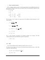
Laboratory set-up
A schematic diagram of the laboratory set-up is shown in Fig. 1.
Electromagnet
PC
Sensor
Sphere
Frame
RT-DAC4/PCI
board
Power
supply
Fig. 1. MLS laboratory set-up
MLS User’s Manual
-3-
One obtains the mechanical unit with power supply and interface to a PC and the
dedicated RTDAC4/PCI I/O board configured in the Xilinx technology. The software
operates in real time under MS Windows 98/NT/ 2000/XP using MATLAB 6.5 , RTW
and RTWT toolboxes.
Control experiments are programmed and executed in real-time in the MATLAB/Simulink
environment. Thus it is strongly recommended to a user to be familiar with the RTW and
RTWT toolboxes. One has to know how to use the attached models and how to create his
own models.
The control software for the MLS is included in the MLS toolbox. This toolbox uses the
RTWT and RTW toolboxes from MATLAB.
MLS Toolbox is a collection of M-functions, MDL-models and C-code DLL-files that
extends the MATLAB environment in order to solve MLS modelling, design and control
problems. The integrated software supports all phases of a control system development:
• on-line process identification,
• control system modelling, design and simulation,
• real-time implementation of control algorithms.
MLS Toolbox is intended to provide a user with a variety of software tools enabling:
• on-line information flow between the process and the MATLAB environment,
• real-time control experiments using demo algorithms,
• development, simulation and application of user-defined control algorithms.
MLS Toolbox is distributed on a CD-ROM. It contains software and the MLS User’s
Manual. The Installation Manual is distributed in a printed form.
1.2
Hardware and software requirements.
Hardware
Hardware installation is described in the Assembling manual. It consists of:
• Electromagnet
• Ferromagnetic objects
• Position sensor
• Current sensor
• Power interface
• RTDAC4/PCI measurement and control I/O board
• Pentium or AMD based personal computer.
Software
For development of the project and automatic building of the real-time program is required.
The following software has to be properly installed on the PC:
• MS Windows 2000 or Windows XP. MATLAB version 6.5 with Simulink 5.
Signal Processing Toolbox and Control Toolbox from MathWorks Inc. to develop
the project.
• Real Time Workshop to generate the code.
• Real Time Windows Target toolbox.
MLS User’s Manual
-4-
•
•
1.3
Features of MLS
•
•
•
•
•
•
•
•
1.4
Aluminium construction
Two ferromagnetic objects (spheres) with different weight
Photo detector to sense the object position
Coil current sensor
A highly nonlinear system ideal for illustrating complex control algorithms
None friction effects are present in the system
The set-up is fully integrated with MATLAB/Simulink and operates in real-time
in MS Windows 98/2000/XP
The software includes complete dynamic models.
Typical teaching applications
•
•
•
•
•
•
•
•
1.5
The MLS toolbox which includes specialised drivers for the MLS System, These
drivers are responsible for communication between MATLAB and the RTDAC4/PCI measuring and control board.
MS Visual C++ to compile the generated code.
System Identification
SISO, MISO, BIBO controllers design
Intelligent/Adaptive Control
Frequency analysis
Nonlinear control
Hardware-in-the-Loop
Real-Time control
Closed Loop PID Control
Software installation
Insert the installation CD and proceed step by step following displayed commands.
MLS User’s Manual
-5-
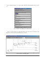
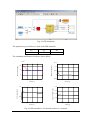
2 ML Main Window
The user has a rapid access to all basic functions of the MLS System from the MLS Control
Window. In the Matlab Command Window type:
ML_Main
and then the Magnetic Levitation Main window opens (see Fig. 2).
Fig. 2. The Magnetic Levitation Main window
In the ML Main window one can find: testing tools, drivers, models and demo applications.
You can see a number of pushbuttons ready to use.
The ML Main window shown in Fig. 2 contains four groups of the menu items:
•
Tools – identification
•
RTWT Device Driver – MagLev device driver
•
Simulation model and controllers
•
Real-time experiments – levitation
Section 2 is divided into four subsections. Under each button in the ML Main window one
can find the respective portion of software corresponding to the problem announced by the
button name. These problems are described below in four consecutive subsections.
MLS User’s Manual
-6-
2.1
Identification
If we click the identification button the following window (see Fig. 3) opens. There are the
default values of all parameters defined by the manufacturer. Nevertheless, a user is
equipped with a number of identification tools. He can perform the identification
procedures to verify and if necessary modify static and dynamic characteristics of MLS.
Fig. 3. The identification window
Four identification steps have been preprogrammed. They are described below.
2.1.1 Sensor
In this subsection the position sensor characteristics is identified.
If you click the Sensor button the following window opens (see Fig. 4)
Fig. 4. Sensor signal in [V] vs. the sphere distance from the electromagnet in [mm]
MLS User’s Manual
-7-
The following procedure is required to identify the characteristics.
1. Screw in the screw bolt into the seat.
2. Screw in the black sphere and lock it by the butterfly nut. Notice, that the sphere
is fixed to the frame!
3. Turn round the screw so the sphere be in touch with the bottom of the
electromagnet.
4. Switch on the power supply and the light source.
5. Start the measuring and registration procedure. It consists of the following steps:
6. Push the Measure button – the voltage from the position sensor is stored and
displayed as Measured value [V]. One can correct this value by measuring it
again.
Push the Add button – the measured value is added to the list. A rotation
number value is automatically enlarged by one (see Fig. 5).
Fig. 5. Characteristics of the sphere position sensor
Manually make one full rotation of the screw.
Repeat three last steps so many times as none change in the voltage vs.
position characteristics is observed.
7. Push the Export Data button – the data are written to the disc (see Fig. 6). Data
are stored in the ML_Sensor.mat file as the SensorData structure with the
following signals: Distance_mm, Distance_m and Sensor_V.
In the Simulink real-time models the above characteristics is used as a Look-Up-Table
model. The block named Position scaling is located inside the device driver block of MLS
(see Fig. 7). Notice, that the characteristics shows meters vs. Volts. In Fig. 6 there were
shown Volts vs. meters. It is obvious that we require the inverse characteristics because we
need to define the output as the position in meters.
MLS User’s Manual
-8-
5
4.5
4
Sensor signal [V]
3.5
3
2.5
2
1.5
1
0.5
0
0.002
0.004
0.006
0.008
0.01
Distance [m]
0.012
0.014
0.016
0.018
Fig. 6. The sensor characteristics after being measured and exported to the disc
Position scaling
[V] to [m]
Fig. 7. The Simulink Look Up Table model representing the position sensor characteristics
If we click this block the window shown in Fig. 8 opens. Any time you like to modify
the sensor characteristics you can introduce new data related to the voltage measured by the
sensor. The voltage corresponds to the distance of the sphere set by a user while the
identification procedure is performed. The sensor characteristics is loaded from the
ML_sensor.dat file which has been created during the identification procedure. If the curve
of the Position scaling block is not visible please load the file with data.
The sensor characteristics can be approximated by a polynomial of a given order. For
example, we can use a fifth order polynomial.
P ( x ) = p5 x 5 +
+ p0
p5 = −25697073504.59,
p4 = 1245050011.25,
p1 = −150.21 and p0 = 5.015.
MLS User’s Manual
p3 = −18773635.92,
p2 = 79330.24,
-9-
Fig. 8. Look-Up Table to be fulfilled with vectors of input and output values
The approximated polynomial (the red line) is shown in Fig. 9. The polynomial
approximation will be not used in this manual due to the fact that the entire model is built
in Simulink. Therefore we recommend to model the characteristics as a Look-Up Table
block (see Fig. 7 and Fig. 8).
5.5
5
4.5
Sensor signal [V]
4
3.5
3
2.5
2
1.5
1
0.5
0
0.002
0.004
0.006
0.008
0.01
Distance [m]
0.012
0.014
0.016
0.018
Fig. 9. The sensor characteristics approximated by the fifth order polynomial
MLS User’s Manual
-10-
2.1.2
Actuator static mode
In this subsection we examine static features of the actuator i.e. the electromagnet.
Notice, that the sphere is not present!
Click the Actuator static mode button and the window shown in Fig. 10 opens.
Fig. 10. Identification window of a static current/voltage characteristics
Now, we can perform button by button the operations depicted in Fig. 10. We begin from
the Build model for data acquisition button. The window of the real-time task shown in
Fig. 11 opens and the RTW build command is executed (the executable code is created).
Fig. 11. Real-time model built to examine the current in the electromagnetic coil
Click the Set control gain button. It results in activation of the model window and the
following message is displayed (see Fig. 12):
MLS User’s Manual
-11-
Fig. 12. Message – Set the “Control Gain”
In Fig. 11 one can notice the Control signal block. In fact the control signal increases
linearly. We can modify the slope of this signal changing the Control Gain value.
Click the Data acquisition button. Within 10 seconds data are acquired and stored in the
workspace.
Click the Data analysis button. The collected values of the coil current are displayed in
Fig. 13.
Fig. 13. Current in the electromagnetic coil
The characteristics is linear except a small interval at the beginning. We can locate the
cursor at the point where a new line slope starts (see the red line in the picture). We can
move the cursor in two ways: by writing down a value into the edition window or by
drugging the slider. In this way the current characteristics is prepared to be analyzed in the
next step. The line is divided into two intervals: the first – from the beginning of
measurements to the cursor and the second – from the cursor to the end of measurements.
After setting the cursor position, consequently, click the Analyze button. The following
message (see Fig. 14) appears. We obtain the dead zone values corresponding to the
control and current. The constants a and b of the linear part are the parameters of the line
equation: i (u ) = a u + b .
MLS User’s Manual
-12-
Fig. 14. Coefficients of the actuator characteristics
These parameters, namely: u MIN = 0.00498 , x3MIN = 0.03884 , k i = 2.5165 and ci = 0.0243
are going to be used in the simulation model in section 2.3.1 (see the differential equations
parameters).
To obtain a family of static characteristics for linear controls with different slopes we
repeat the following experiment. We apply a PWM voltage signal in the time interval from
0 to 10 s. The PWM duty cycles for the subsequent ten experiments are varying linearly in
the ranges: [0, 0.1], [0, 0.2], ..., [0, 1.0] (see Fig. 16 ).
1
0.9
0.8
Control - PWM duty
0.7
0.6
0.5
0.4
0.3
0.2
0.1
0
0
1
2
3
4
5
Time [s]
6
7
8
9
10
Fig. 15. Family of the input (PWM) characteristics
Consequently, we obtain diagrams of the currents corresponding to ten experiment (see
Fig. 16). Each characteristics is approximated by a polynomial of the first order. Finally the
entire current vs. PWM duty cycle relation is depicted (black points) in Fig. 17. The red
line represents the linear approximation of measurements. We obtain the following
numerical values of linear characteristics:
i (u ) = k i u + c ; a = 2.60798876298869, b = −0.01077522109792.
The constant c is obtained for u = 0 . The family of linear characteristics is used to obtain
the coefficients k i vs. control u.
MLS User’s Manual
-13-
3
2.5
Current [A]
2
1.5
1
0.5
0
-0.5
0
1
2
3
4
5
Time [s]
6
7
8
9
10
Fig. 16. Family of the output (current) characteristics
3
2.5
Current [A]
2
1.5
1
0.5
0
-0.5
0
0.1
0.2
0.3
0.4
0.5
0.6
Control - PWM duty
0.7
0.8
0.9
1
Fig. 17. Current vs. PWM duty cycle
2.1.3
Minimal control
In this subsection we examine the minimal control to cause a forced motion of the
sphere from the supporting structure (tablet) toward the electromagnet against the gravity
force. Notice, that in this experiment the sphere is not levitating! It is kept nearby the
electromagnet by the supporting structure.
Click the Minimal control button and the window shown in Fig. 18 opens.
MLS User’s Manual
-14-
Fig. 18. Window to identify the minimal control vs. distance
(between the sphere and electromagnet)
Now, we proceed button by button the operations depicted in Fig. 18 similarly to the
procedure described in the previous subsection. We begin from the Build model for data
acquisition button. The window of the real-time task shown in Fig. 19 opens.
Fig. 19. Real-time model built to examine the minimal electromagnetic force
Click the Set control gain button. It results in activation of the model window and the
following message is displayed (see Fig. 20).
Fig. 20. Message – set the “Control Gain”
It means that we can set a duty cycle of the control PWM signal. The sphere is located
on the support and the experiment starts. Click the Data acquisition button. A forced
motion of the ball toward the electromagnet begins.
MLS User’s Manual
-15-
Click the Data analysis button. The collected values of the ball position are displayed
in Fig. 21.
Fig. 21. The sphere motion
The sphere motion is visible. We can locate the cursor at the point slightly before a
position jump occurs (takes place) (see the red line in the picture). We can move the cursor
in two ways: by writing down a value into the edition window or by drugging the slider. In
this way the acquired data are prepared to be analyzed in the next step.
After setting the cursor position, consequently, click the Analyze button. The following
message (see Fig. 22) appears. This information means that the sphere located 15.82 mm
from the electromagnet begins to move toward it when the PWM control over-crosses the
0.49485 duty cycle value.
Fig. 22. Message of the experiment results
MLS User’s Manual
-16-
2.1.4
Actuator dynamic mode
In this subsection we examine dynamic features of the actuator i.e. the electromagnet. It
means that the moving sphere generates an electromotive force (EMF). EMF diminishes
the current in the electromagnet coil. Click the Actuator static mode button and the window
shown in Fig. 23 opens.
Fig. 23. Identification window of a dynamic current/voltage characteristics
A user should perform three experiments: without the sphere (Without ball), with the
sphere on the supported structure (Ball on the tablet) and with the sphere fixed to the rigid
screw (Ball fixed).
We begin from the Build model for data acquisition button. The window of the realtime task shown in Fig. 24 opens. We have to set the control gain. If we are going to
modify the control magnitude then we set the default gain to 1 and the subsequent duty
cycles to: 0.25, 0.5, 0.75 and 1. Click the Data acquisition button and save data under a
given file name.
Fig. 24. Real-time model built to examine EMF influence on the coil current
MLS User’s Manual
-17-
Click the Data analysis button. It calls the ml_find_curr_dyn.m file. The following
window opens (see Fig. 25). The parameters optimization procedure starts. The
optimization routine is based on the mlm_current.mdl model.
When ml_find_curr_dyn.m runs the optimization function fminsearch is executed.
Fminsearch uses the ml_opt_current.m file.
The ki and fi parameters are iteratively changed during the optimization procedure. The
current curve is fitted four times. This is due to the control signal form.
0.7
0.6
Current [A]
0.5
0.4
0.3
0.2
0.1
measured current
modeled current
0
0
0.02
0.04
0.06
0.08
0.1
Time [s]
0.12
0.14
0.16
0.18
Fig. 25. Current curve – the fitting result of the optimization procedure
Finally the information about the mean values is displayed (see Fig. 26). The advanced
user can use the functions code to perform a detailed analysis.
Fig. 26. Optimization results
MLS User’s Manual
-18-
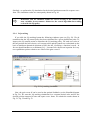
2.2
MagLev device drivers
The driver is a software go-between for the real-time MATLAB environment and the
RT-DAC4/PCI acquisition board. The control and measurements are driven. Click the
RTWT Device Drivers button in the Magnetic Levitation Main window. The following
window opens (see Fig. 27).
Fig. 27. RTWT MagLev device driver window
Notice that the scope block writes data to the MLExpData variable defined as a structure
with time. The structure consists of the following signals: Position [m], Velocity [m/s],
Current [A], Control [PWM duty 0÷1]. The interior of the Magnetic Levitation System
block, it means the interior of the driver block is shown in Fig. 28.
Fig. 28. Interior of the driver block
MLS User’s Manual
-19-
In fact there are two drivers: ML_AnalogInputs and ML_PWM. There are also two
characteristics: the ball position [m] vs. the position sensor voltage [V] and the coil current
vs. the current sensor voltage [V]. The driver uses functions which communicates directly
with a logic stored at the RT-DAC4/PCI board. When one wants to build his own
application one can copy this driver to a new model.
Do not introduce any changes inside the original driver. They can be
introduced only inside its copy!!! Make a copy of the installation CD.
The Simulink Look-Up-Table model named Position scaling (see Fig. 7) representing the
position sensor characteristics has been already described. Now let us present the second
Simulink Look-Up-Table model named Current scaling (see Fig. 29).
Current scalling
[V] to [A]
Fig. 29. The Simulink Look-Up-Table model representing the current sensor characteristics
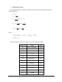
To build the above characteristics it is necessary to measure the current of the
electromagnet coil. The algorithm in the computer is the source of the desired value of the
control in the form of the voltage PWM signal. This PWM is the input voltage signal
transferred to the LMD18200 chip of the power interface. Due to a high frequency of the
PWM signal the measured current values correspond to the average current value in the
coil. This characteristics has been built by the manufacturer. It is not recommended to
repeat measurements by a user because to do so one must unsolder the input wires of the
electromagnet. On the basis of the data given in the table below one can generate his own
characteristics. For a fixed PWM frequency and a variable duty cycle the coil amperage is
measured. The measured data are given below in the table.
PWM duty cycle
0
0.1
0.2
0.3
0.4
0.5
0.6
0.7
0.8
0.9
1
MLS User’s Manual
amperage [A]
0
0.25
0.51
0.77
1.02
1.28
1.52
1.74
1.99
2.21
2.43
voltage [V]
0.374811
0.262899
0.510896
0.752465
0.993620
1.229133
1.459294
1.651424
1.875539
2.076814
2.269865
-20-
The current [A] vs. voltage [V] characteristics is shown in Fig. 30.
2.5
Current [A]
2
1.5
1
0.5
0
0
0.5
1
1.5
Measured signal [V]
2
2.5
Fig. 30. Current vs. voltage characteristics approximated by the red curve
The characteristic can be approximated by a polynomial of the second order:
I (U ) = a2U 2 + a1U + a0
where:
I – current,
U – voltage from the A/D converter
a0 , a1 , a 2 - identified parameters of the polynomial
a 2 = 0.0168
a1 = 1.0451
a0 = −0.0317
MLS User’s Manual
-21-
2.3
Simulation Model & Controllers
Click the Simulation Model & Controllers button in the Magnetic Levitation Main
window. The following window opens (see Fig. 31).
Fig. 31. Simulation Model & Controllers window
2.3.1
Open Loop
Simulink model
Next, you can click the first Open Loop button. The following window opens (see Fig.
32). Notice that the scope block writes data to the MLSimData variable defined as a
structure with time. The structure consists of the following signals: Position [m], Velocity
[m/s], Current [A], Control [PWM duty 0÷1].
Fig. 32. Open-loop simulation
MLS User’s Manual
-22-
If you click the Magnetic Levitation model block the following mask opens (see Fig.
33).
Fig. 33. Mask of the Magnetic Levitation model
In Fig. 32 enter into the File option and choose Look under mask. The interior of the
Magnetic Levitation model block shown in Fig. 34 opens.
Fig. 34. Interior of the ML model
MLS User’s Manual
-23-
Notice two integrator blocks in Fig. 34. In fact we deal with third order dynamical
system. The third integrator related to the coil current is visible in Fig. 35.
Fig. 35. Interior of the Current model block
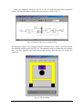
The Simulink model is also equipped with the animation block. When a simulation starts
the following window opens (see Fig. 36). The animation screen is updated in every sample
time. All state variables: the ball position and velocity, and also the coil current are
animated.
Fig. 36. ML animation
MLS User’s Manual
-24-
Mathematical model
The Simulink model is consistent with the following nonlinear mathematical model
Model nieliniowy
x1 = x2
Fem
+g
m
1
x3 =
(kiu + ci − x3 )
f i ( x1 )
x2 = −
Fem = x32
FemP1
x
exp(− 1 )
FemP 2
FemP 2
f i ( x1 ) =
f iP1
x
exp(− 1 )
f iP 2
f iP 2
where:
x1 ∈ [0, 0.016] ,
x2 ∈ ℜ ,
x3 ∈ [ x3MIN , 2.38]
u ∈ [u MIN , 1]
The parameters of the above equations are given in the table below
MLS User’s Manual
Parameters
Values
Units
m
0.0571 (big ball)
[kg]
g
9.81
[m/s2]
Fem
function of x1 and x3
[N]
FemP1
1.7521⋅10-2
[H]
FemP 2
5.8231⋅10-3
[m]
f i ( x1 )
function of x1
[1/s]
f iP1
1.4142⋅10-4
[m·s]
f iP 2
4.5626⋅10-3
[m]
ci
0.0243
[A]
ki
2.5165
[A]
x3MIN
0.03884
[A]
u MIN
0.00498
-25-
The electromagnetic force vs. position diagram is shown in Fig. 37 and the electromagnetic force vs. coil current diagram is shown respectively in Fig. 38.
3
Electromagnetic force [N]
2.5
2
1.5
1
0.5
0
0
0.002 0.004 0.006 0.008 0.01 0.012 0.014 0.016 0.018
Position [m]
0.02
Fig. 37. Electromagnetic force vs. position. The gravity force of the big ball (dashed
horizontal line) is crossing the curve at the 0.009 m distance from the electromagnet
3.5
Electromagnetic force [N]
3
2.5
2
1.5
1
0.5
0
0
0.5
1
1.5
Coil current [A]
2
2.5
Fig. 38. Electromagnetic force vs. coil current. The gravity force of the big ball (dashed
horizontal line) is crossing the curve at the 0.9345 A coil current
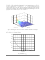
The electromagnetic force depends on two variables: the ball distance from the
electromagnet and the current in the electromagnetic coil. This is clearly presented in Fig.
MLS User’s Manual
-26-
37 and Fig. 38. We can show these dependencies in three dimensional space (see Fig. 39).
The ball is stabilized at [x1 , x 2 , x3 ] = col(9⋅10−3, 0, 9.345⋅10−1). It means that the ball
velocity remains equal to zero. The ball is levitating kept at the 9 mm distance from the
bottom of the electromagnet. The 0.9345 A current flowing through the magnetic coil is the
appropriate value to balance the gravity force of the ball.
Electromagnetic force [N]
15
10
5
0
3
0.02
2
0.015
0.01
1
0.005
0
Coil current [A]
0
Position [m]
Fig. 39. Electromagnetic force vs. coil current and distance from the electromagnet.
In Fig. 40 the f i ( x1 ) diagram is shown.
0.035
0.03
0.025
fi(x1)
0.02
0.015
0.01
0.005
0
0
0.002 0.004 0.006 0.008 0.01 0.012 0.014 0.016 0.018
Position [m]
0.02
Fig. 40. Function f i ( x1 )
MLS User’s Manual
-27-
Linear continuous model
ML is a highly nonlinear model. It can be approximated in an equilibrium point by a
linear model. The linear model can be described by three linear differential equations of the
first order in the form:
x = Ax + Bu
y = Cx
0
1
0
0
A = a2,1 0 a2,3 ,
a3,1 0 a3,3
B= 0
b3
The elements of the A matrix are expressed by the nonlinear model parameters in the
following way:
x10
x 2 F 1 − FemP 2
a2,1 = 30 emP
e
2
m FemP
2
x10
a2 , 3
−
2x F
= − 30 emP1 e FemP 2
m FemP 2
a3,1 = −(ki u + ci − x30 )
x10
−
f
− iP2 1 e fiP 2
f iP 2
2
a3,3 = − f i −1 ( x10 )
b3 = k i f i −1 ( x10 )
The C vector elements correspond to an applied controller. For example, The PID
controller shown in the next subsection requires C in the form:
C = [1 0 0] .
2.3.2
PID
If you click the PID button the following windows open (see Fig. 41).
The interior of the Magnetic Levitation model block has been shown in Fig. 34. The PID
controller is built in the form:
u (t ) = K P ⋅ e(t ) + K I e(t )dt + K D
d
e(t )
dt
e(t ) = x(t ) − x0 (t )
MLS User’s Manual
-28-
Fig. 41. PID simulation
The parameters given bellow are used in the PID controller.
KP
130
KI
500
KD
6
The simulated stabilization results are shown below.
x 10
-3
0.15
Ball velocity [m/s]
Ball position [m]
10
9
8
0.1
0.05
0
-0.05
0
0.5
1
T ime [s]
1.5
0.5
1
T ime [s]
1.5
2
0
0.5
1
T ime [s]
1.5
2
0.8
Control - PWM duty
1.5
Coil current [A]
0
1
0.5
0
0
0.5
1
T ime [s]
1.5
2
0.6
0.4
0.2
0
Fig. 42. PID simulation – the desired position is a constant.
MLS User’s Manual
-29-
x 10
-3
x 10
2
Ball velocity [m/s]
Ball position [m]
11
10
9
8
7
1
0
-1
-2
0
1
2
T ime [s]
3
4
1.05
0
1
2
T ime [s]
0
1
2
T ime [s]
3
4
0.4
Control - PWM duty
Coil current [A]
-3
1
0.95
0.9
0.35
0.85
0
1
2
T ime [s]
3
0.3
4
3
4
Fig. 43. PID simulation – the desired position is in a sine wave form.
x 10
-3
0.15
Ball velocity [m/s]
Ball position [m]
11
10
9
8
7
0.1
0.05
0
-0.05
0
1
2
T ime [s]
3
4
1
2
T ime [s]
3
4
0
1
2
T ime [s]
3
4
0.8
Control - PWM duty
Coil current [A]
1.5
0
1
0.5
0
0.6
0.4
0.2
0
0
1
2
T ime [s]
3
4
Fig. 44. PID simulation – the desired position is in a square wave form.
MLS User’s Manual
-30-
2.3.3
LQ
If you click the LQ button the following windows open (see Fig. 45).
Fig. 45. LQ simulation
The continuous LQ regulator is depicted on the basis of ml_model4lq.mdl (see Fig. 46).
The user can use two files
• ML_calc_steady_state.m
•
ML_calc_lq.m
The first one calculates the equilibrium point of the system. The second one calculates the
LQ controller parameters using linmod and lqr. linmod obtains linear models from systems
of ordinary differential equations. In the ML_calc_lq.m file we encounter the following
command:
[A, B, C, D] = linmod('ml_model4lq');
Fig. 46. Ml_model4lq.mdl to extract an LQ regulator
MLS User’s Manual
-31-
The state-space linear model of the system of ordinary differential equations described
in the block diagram 'model4lq' is returned in the form of the A, B, C, D matrices. The state
variables and inputs are set to the defaults specified in the block diagram. Having obtained
the linear model calculated at x10, x 20, x30 equilibrium point for the assumed value u 0 of
the control we are ready to calculate the K gains of the LQ controller. We only need to
assume the Q and R matrices. From the ML_calc_lq.m file we have
Q=eye(3,3); Q(1,1)= 300; Q(2,2)= 0.001; Q(3,3) = 10; R=10.5;
The following assumptions corresponding to the Q and R weighting matrices have to be
satisfied:
Q≥0 R>0
The following command from the ML_calc_lq.m file:
[K,S,E] = lqr(A,B,Q,R)
calculates the optimal gain matrix K such that the state-feedback law u = −Kx minimizes
dx
the cost function ( x′Qx + u ′Ru )dt subject to the state dynamics
= Ax + Bu .
dt
Now, the gain vector K can be used as the optimal feedback (see the Simulink diagram in
Fig. 45). We start the LQ simulation for a constant desired value and for the desired
position assumed in a sine wave form. We obtain the results shown in Fig. 47 and Fig. 48.
x 10
-3
0.03
Ball velocity [m/s]
Ball position [m]
9.5
9
8.5
0.02
0.01
0
-0.01
0
0.5
1
T ime [s]
1.5
0.5
1
T ime [s]
1.5
2
0
0.5
1
T ime [s]
1.5
2
0.4
Control - PWM duty
Coil current [A]
1
0
0.9
0.8
0.7
0.3
0.2
0.1
0
0
0.5
1
T ime [s]
1.5
2
Fig. 47. LQ simulation – the desired position is a constant
MLS User’s Manual
-32-
x 10
-3
0.04
Ball velocity [m/s]
Ball position [m]
11
10
9
8
0.02
0
-0.02
7
0
1
2
T ime [s]
3
1
2
T ime [s]
3
4
0.8
Control - PWM duty
1.1
Coil current [A]
0
4
1
0.9
0.8
0.7
0.6
0.4
0.2
0
0
1
2
T ime [s]
3
4
0
1
2
T ime [s]
3
4
Fig. 48. LQ simulation – the desired position is in a sine wave form
x 10
-3
0.15
Ball velocity [m/s]
Ball position [m]
11
10
9
8
7
0.1
0.05
0
-0.05
0
1
2
T ime [s]
3
4
1
2
T ime [s]
3
4
0
1
2
T ime [s]
3
4
0.8
Control - PWM duty
Coil current [A]
1.5
0
1
0.5
0
0.6
0.4
0.2
0
0
1
2
T ime [s]
3
4
Fig. 49. LQ simulation – the desired position is in a square wave form
MLS User’s Manual
-33-
Similarly, we perform the LQ simulation for the desired position assumed in a square wave
form. The simulation results are consequently shown in Fig. 49.
Remember that the obtained results are correct as long as the control and
state variables do not saturate. Otherwise, the control algorithm has nothing
to do with the LQ policy.
2.3.4
LQ tracking
If you click the LQ tracking button the following windows open (see Fig. 50). We do
remember that the LQ control policy has been calculated for a given equilibrium point. To
improve the LQ control action we introduce the LQ tracking policy. For each new value of
the ball position the ball velocity, coil current values and the control are recalculated on the
basis of nonlinear dynamical equations of ML (the ML_GetStState s-function is used). In
fact we should introduce a no-stationary LQ – it means solve the Riccati equation for every
new equilibrium point to obtain a new value of the gain vector K.
Fig. 50. LQ tracking simulation
Now, the gain vector K can be used as the optimal feedback (see the Simulink diagram
in Fig. 50). We start the LQ tracking simulation for a constant desired value and for the
desired position assumed in sine and square wave forms. We obtain the results shown in
Fig. 51, Fig. 52 and Fig. 53.
MLS User’s Manual
-34-
x 10
-3
0.03
Ball velocity [m/s]
Ball position [m]
9.5
9
8.5
0.02
0.01
0
-0.01
0
0.5
1
T ime [s]
1.5
0.5
1
T ime [s]
1.5
2
0
0.5
1
T ime [s]
1.5
2
3
4
0.4
Control - PWM duty
Coil current [A]
1
0
0.9
0.8
0.7
0.3
0.2
0.1
0
0
0.5
1
T ime [s]
1.5
2
Fig. 51. LQ tracking simulation – the desired position is a constant
x 10
-3
0.03
Ball velocity [m/s]
Ball position [m]
11
10
9
8
7
1
2
T ime [s]
3
0
4
0
1.1
1
2
T ime [s]
0.8
Control - PWM duty
Coil current [A]
0.01
-0.01
0
1
0.9
0.8
0.7
0.02
0
1
2
T ime [s]
3
4
0.6
0.4
0.2
0
0
1
2
T ime [s]
3
4
Fig. 52. LQ tracking simulation – the desired position is in a sine wave form.
MLS User’s Manual
-35-
x 10
-3
0.15
Ball velocity [m/s]
Ball position [m]
11
10
9
8
7
0.1
0.05
0
-0.05
0
1
2
T ime [s]
3
4
1
2
T ime [s]
3
4
0
1
2
T ime [s]
3
4
0.8
Control - PWM duty
Coil current [A]
1.5
0
1
0.5
0
0.6
0.4
0.2
0
0
1
2
T ime [s]
3
4
Fig. 53. LQ tracking simulation – the desired position is in a square wave form.
MLS User’s Manual
-36-
2.4
Levitation
All simulation experiments can be repeated as real-time experiments. In this way one
can verify accuracy of modelling. If we double click the levitation button in the ML Main
window the following window opens (see Fig. 54).
Fig. 54. Experimental controllers
Now, we can choose the controller we are interested in. We start from the PID control.
2.4.1
PID
Double click the PID button. The real-time PID controller opens (see Fig. 55). The results
of the real-time experiment are shown in: Fig. 56, Fig. 57 and Fig. 58.
Fig. 55. PID real-time experiment.
MLS User’s Manual
-37-
x 10
-3
0.1
Ball velocity [m/s]
Ball position [m]
11
10
9
0.05
0
-0.05
8
-0.1
0
1
2
T ime [s]
3
4
1
2
T ime [s]
3
4
0
1
2
T ime [s]
3
4
1
Control - PWM duty
Coil current [A]
1.4
0
1.2
1
0.5
0.8
0
0
1
2
T ime [s]
3
4
Fig. 56. PID real-time experiment. The desired position as a constant.
x 10
-3
0.1
Ball velocity [m/s]
Ball position [m]
11
10
9
8
0.05
0
-0.05
7
-0.1
0
1
2
T ime [s]
3
4
0
2
T ime [s]
3
4
1
Control - PWM duty
Coil current [A]
1.2
1
1
0.5
0
0.8
0
1
2
T ime [s]
3
4
0
1
2
T ime [s]
3
4
Fig. 57. PID real-time experiment. The desired position in a sine wave form.
MLS User’s Manual
-38-
x 10
-3
0.3
Ball velocity [m/s]
Ball position [m]
12
10
8
6
0.1
0
-0.1
0
1
2
T ime [s]
3
4
1.4
1.4
1.2
1.2
Coil current [A]
Coil current [A]
0.2
1
0.8
0.6
0
1
2
T ime [s]
3
4
0
1
2
T ime [s]
3
4
1
0.8
0.6
0
1
2
T ime [s]
3
4
Fig. 58. PID real-time experiment. The desired position in a square wave form.
2.4.2
LQ
Double click the LQ button. The real-time LQ controller opens (see Fig. 59). The results
of the real-time experiment are shown in: Fig. 60, Fig. 61 and Fig. 62.
Fig. 59. LQ real-time experiment.
MLS User’s Manual
-39-
x 10
-3
0.1
Ball velocity [m/s]
Ball position [m]
11
10
9
0.05
0
-0.05
8
-0.1
0
1
2
T ime [s]
3
4
1
2
T ime [s]
3
4
0
1
2
T ime [s]
3
4
0.8
Control - PWM duty
Coil current [A]
1.4
0
1.2
1
0.8
0.6
0.4
0.2
0.6
0
0
1
2
T ime [s]
3
4
Fig. 60. LQ real-time experiment. The desired position as a constant.
x 10
-3
0.1
Ball velocity [m/s]
Ball position [m]
11
10
9
8
0.05
0
-0.05
-0.1
7
0
1
2
T ime [s]
3
4
1
2
T ime [s]
3
4
0
1
2
T ime [s]
3
4
0.8
Control - PWM duty
Coil current [A]
1.2
0
1
0.8
0
1
2
T ime [s]
3
4
0.6
0.4
0.2
0
Fig. 61. LQ real-time experiment. The desired position in a sine wave form.
MLS User’s Manual
-40-
x 10
-3
0.2
Ball velocity [m/s]
Ball position [m]
12
10
8
6
0
-0.1
-0.2
0
1
2
T ime [s]
3
4
0
1
2
T ime [s]
3
1
2
T ime [s]
3
4
1
Control - PWM duty
1.5
Coil current [A]
0.1
1
0.5
0.5
0
0
0
1
2
T ime [s]
3
4
0
4
Fig. 62. LQ real-time experiment. The desired position in a square wave form.
2.4.3
LQ tracking
Double click the LQ tracking button. The real-time LQ tracking controller opens (see
Fig. 63). The results of the real-time experiment are shown in Fig. 64, Fig. 65 and Fig. 66.
Fig. 63. LQ tracking real-time experiment.
MLS User’s Manual
-41-
x 10
-3
0.01
Ball velocity [m/s]
Ball position [m]
10
9.5
9
8.5
0
1
2
T ime [s]
3
0
-0.01
-0.02
-0.03
4
1
2
T ime [s]
3
4
0
1
2
Time [s]
3
4
1
Control - PWM duty
1.4
Coil current [A]
0
1.2
1
0.8
0.6
0.4
0.2
0.8
0
1
2
T ime [s]
3
4
Fig. 64. LQ tracking real-time experiment. The desired position as a constant.
0.02
Ball velocity [m/s]
Ball position [m]
0.015
0.01
0.005
0.01
0
-0.01
0
1
2
T ime [s]
3
4
0
2
T ime [s]
3
4
1
2
T ime [s]
3
4
0.8
Control - PWM duty
1.4
Coil current [A]
1
1.2
1
0.8
0.6
0.4
0.2
0
0.6
0
1
2
T ime [s]
3
4
0
Fig. 65. LQ tracking real-time experiment. The desired position in a sine wave form.
MLS User’s Manual
-42-
x 10
-3
0.2
Ball velocity [m/s]
Ball position [m]
12
10
8
6
4
0
-0.1
-0.2
0
1
2
T ime [s]
3
4
0
1
2
T ime [s]
3
4
0
1
2
T ime [s]
3
4
1
Control - PWM duty
2
Coil current [A]
0.1
1.5
1
0.5
0
0.5
0
0
1
2
T ime [s]
3
4
Fig. 66. LQ tracking real-time experiment. The desired position in a square wave form.
MLS User’s Manual
-43-
3 Description of the Magnetic Levitation class properties
The MagLev is a MATLAB class, which gives the access to all the features of the
RT-DAC4/PCI board supported with the logic for the MLS model. The RT-DAC4/PCI
board is an interface between the control software executed by a PC computer and the
power-interface electronic of the modular servo model. The logic on the board contains the
following blocks:
•
•
•
PWM generation block – generates the Pulse-Width Modulation output signal.
Simultaneously the direction signal and the brake signal are generated to control the
power interface module. The PWM prescaler determines the frequency of the PWM
wave;
power interface thermal status –the thermal status can be used to disable the
operation of the overheated actuator unit;
interface to the on-board analog-to-digital converter. The A/D converter is applied to
measure the position of the ball (light sensor) and to measure the coil current of the
actuator.
All the parameters and measured variables from the RT-DAC4/PCI board are accessible by
appropriate properties of the MagLev class.
In the MATLAB environment the object of the MagLev class is created by the command:
object_name = MagLev;
for example ml = maglev;
The get method is called to read a value of the property of the object:
property_value = get( object_name, ‘property_name’ );
The set method is called to set new value of the given property:
set( object_name, ‘property_name’, new_property_value );
The display method is applied to display the property values when the object_name is
entered in the MATLAB command window.
This section describes all the properties of the MagLev class. The description consists of
the following fields:
Purpose
Synopsis
Description
Arguments
See
Examples
MLS User’s Manual
Provides short description of the property
Shows the format of the method calls
Describes what the property does and the restrictions subjected
to the property
Describes arguments of the set method
Refers to other related properties
Provides examples how the property can be used
-44-
3.1
BaseAddress
Purpose:
Read the base address of the RT-DAC4/PCI board.
Synopsis:
BaseAddress = get( ml, ‘BaseAddress’ );
Description: The base address of RT-DAC4/PCI board is determined by computer.
Each CML object has to know the base address of the board. When a CML
object is created the base address is detected automatically. The detection
procedure detects the base address of the first RT-DAC4/PCI board
plugged into the PCI slots.
Example:
Create the MagLev object:
ml = MagLev;
Display their properties by typing the command:
ml
Type:
BaseAddress:
Bitstream ver.:
Input voltage:
PWM:
PWM Prescaler:
Thermal status:
Time:
InTeCo ML object
54272 / D400 Hex
x901
[ 0.8451 0.0244 ][V]
[ 0 ]
[ 0 ]
[ 0 ]
0.00 [sec]
Read the base address:
BA = get( ml, ‘BaseAddress’ );
3.2
BitstreamVersion
Purpose:
Read the version of the logic stored in the RT-DAC4/PCI board.
Synopsis:
Version = get( ml, ‘BitstreamVersion’ );
Description: The property determines the version of the logic design of the
RT-DAC4/PCI board. The magnetic levitation models may vary and the
detection of the logic design version makes it possible to check if the
logic design is compatible with the physical model.
3.3
PWM
Purpose:
Set the duty cycle of the PWM wave.
Synopsis:
PWM = get( ml, ‘PWM’ );
set(ml, ‘PWM’, NewPWM );
MLS User’s Manual
-45-
Description: The property determines the duty cycle and direction of the PWM wave.
The PWM wave is used to control the electromagnet so in fact this property
is responsible for the electromagnet control signal. The NewPWM variable is
a scalars in the range from 0 to 1. The value of +1 means the maximum
control, 0.0 means zero control.
See:
PWMPrescaler
Example:
3.4
set( ml, ‘PWM’, [ 0.5 ] );
PWMPrescaler
Purpose:
Determine the frequency of the PWM wave.
Synopsis:
Prescaler = get( ml, ‘PWMPrescaler’ );
set( ml, ‘PWMPrescaler’, NewPrescaler );
Description: The prescaler value can vary from 0 to 16. The 0 value generates the
maximal PWM frequency. The value 16 generates the minimal frequency.
The frequency of the generated PWM wave is given by the formula:
PWMfrequency = 40MHz / 4095* (Prescaler+1)
See:
3.5
PWM
Stop
Purpose:
Sets the control signal to zero.
Synopsis: set( ml, ‘Stop’ );
Description: This property can be called only by the set method. It sets the zero control
of the electromagnet and is equivalent to the set(ml, ‘PWM’, 0) call.
See:
PWM
3.6
Voltage
Purpose:
Read two voltage values.
MLS User’s Manual
-46-
Volt = get( ml, ‘Voltage’ );
Synopsis:
Description: Returns the voltage of two analog inputs. Usually the analog inputs are
applied to measure the ball position and the coil current.
3.7
ThermStatus
Purpose:
Read thermal status flag of the power amplifier.
Synopsis:
ThermSt = get( ml, ‘ThermStatus’ );
Description: Returns the thermal flag of the power amplifier. When the temperature of
a power amplifier is too high the flag is set to 1.
3.8
Time
Purpose:
Return time information.
Synopsis:
T = get( ml, ‘Time’ );
Description: The MagLev object contains the time counter. When a MagLev object is
created the time counter is set to zero. Each reference to the Time property
updates its value. The value is equal to the number of milliseconds which
elapsed since the object was created.
3.9
Quick reference table
Property name
Operation*
BaseAddress
R
Read the base address of the RT-DAC4/PCI board
BitstreamVersion
R
Read the version of the logic design for the
RT-DAC4/PCI board
PWM
R+S
Read/set the parameters of the PWM wave
PWMPrescaler
R+S
Read/set the frequency of the PWM wave
Stop
S
Set the control signal to zero
Voltage
R
Read the input voltages
ThermStatus
R
Read the thermal flags of the power amplifier
Time
R
Read time information
•
Description
R – read-only property, S – allowed only set operation, R+S –property may be
read and set
MLS User’s Manual
-47-