Download Application Developer Manual

Geant4 User’s Documents
Version: Geant4 3.2 June 2001
Geant4 User’s Guide
- For Application Developers 1. Introduction
2. Getting started with Geant4 - Running a simple example
1. How to define the main program
2. How to define a detector geometry
3. How to specify material in the detector
4. How to specify a particle
5. How to specify a physics process
6. How to generate a primary event
7. How to make an executable program
8. How to install and use graphical user interfaces
9. How to execute your program
10. How to visualize the detector and events
3. Practical applications
1. System of Units
2. Class categories/domains
3. Run
4. Event
5. Event generator interface
6. Geometry
7. Materials
8. Electro-magnetic field
9. Particles
10. Physics Processes
11. Tracking
12. Hit
13. Digitization
14. Object persistency
15. User interface commands
16. Visualization
17. Global usage classes
18. Production threshold versus tracking cut
19. User actions classes
20. Example codes
4. Advanced applications
1. More about physics processes
2. More about geometry
3. More about visualization
5. Appendix
1. Summary of built-in commands
2. Tips for the program compilation
3. Histogramming
4. Object-oriented database
5. CLHEP and ANAPHE
6. C++ Standard template library
7. Makefile for Unix
8. Build for MS Visual C++
9. Development and debug tools
10. Particle List in Geant4
About the authors
Geant4 User’s Guide
For Application Developers
1. Introduction
1.1 Scope of this manual
This manual is designed to be a complete introduction to the object-oriented detector simulation toolkit,
Geant4. The manual addresses the needs of the following users of the toolkit:
those who are using Geant4 for the first time,
those who want to develop a serious detector simulation program which can be used in real
experiments.
Geant4 is a completely new detector simulation toolkit, so you don’t need any knowledge of an old
FORTRAN version of GEANT to understand this manual. However, we assume that you have a basic
knowledge of object-oriented programming using C++. If you don’t have any experience with this, you
should first learn it before trying to understand this manual. There are several good, free C++ courses on
the web, which introduce you to this programming language.
Geant4 is a fairly complicated software system, but you don’t need to understand every detail of it
before starting to write a detector simulation program. You will need to know only a small part of it, for
most cases of developing your applications. This manual can be used as one you consult first when you
want to know something new in Geant4.
1.2 How to use this manual
The chapter entitled "Getting started with Geant4 - Running a simple example" gives you a very basic
introduction to Geant4. After reading this chapter, you will be ready to program a simple Geant4
application program. If you are totally new to Geant4, you should read this chapter first.
It is strongly recommended that this chapter be read in conjunction with a Geant4 system running on
your computer. This is especially helpful when you read Chapter 2. To install the Geant4 system on your
computer, please refer to the manual entitled "Installation Guide: For setting up Geant4 in your
computing environment".
The next chapter, entitled "Practical applications", gives you detailed information which is necessary for
writing a serious Geant4 application program. Use of basic Geant4 classes, knowledge of which are
required, is explained with code examples. This chapter is organized according to class categories, also
called class domains, which were defined at the object-oriented analysis stage of the Geant4
development. For an introduction to what is a class category, and object-oriented analysis, please read
the section entitled "Class categories/domains" under this chapter.
The chapter entitled "Advanced applications" provides more advanced information, which is necessary
when developing a more sophisticated application.
About the authors
Geant4 User’s Guide
For Application Developers
Getting started with Geant4
2.1 How to define the main program
2.1.1 What should be written into main()
Geant4 is a detector simulation toolkit, and thus it does not contain a main() routine dedicated to a
specific Geant4 application program. You need to supply your own main() to build a simulation
program. In this section, the minimal items required for a main() routine will be explained.
The G4RunManager class, described in the next subsection, is the Geant4 toolkit class you will have to
deal with first. You must instantiate it, and let it know your demands, which can be:
how your detector should be built
what kinds of physics processes you are interested in
how the primary particle(s) in an event should be produced
any additional demands during the simulation procedures
All of your demands should be stated in your user defined classes, derived from base classes provided
by the Geant4 toolkit. The pointers to your classes should be stored in G4RunManager. The first three
demands should be described in the mandatory user classes, explained in Section 2.1.3. Other
additional demands should be optionally stated in one or more optional user action classes, explained
in Section 2.1.4.
G4RunManager will take care of all of the "kernel" functionalities provided by the Geant4 toolkit.
However, if you want to add a visualization capability and/or a (graphical) user interface capability,
which basically depend on your computer environment, you need to instantiate your favorite driver(s) in
main(). These additional functionalities will be mentioned in Sections 2.9 and 3.16.
2.1.2 G4RunManager
2.1.2.1 Mandates
G4RunManager is the only manager class in the Geant4 kernel which should be explicitly constructed in
the user’s main(). It is the root class of the hierarchy structure of the Geant4 classes and:
1.
2.
3.
4.
5.
controls the major flow of the program
constructs the major manager classes of Geant4,
manages initialization procedures, including methods in the user initialization classes,
manages the event loop(s),
and terminates the major manager classes of Geant4.
The second and the last items are performed automatically in the constructor and the destructor of
G4RunManager, respectively. The third item is done by invoking the initialize() method and the
fourth item is done via the beamOn()method.
2.1.2.2 Major public methods
Detector simulation using Geant4 is an analogy of the real experiment. You construct your detector
setup with the initialize() method, and turn the beam switch on with the beamOn() method. Once
your detector has been constructed, you can do as many runs as you want, i.e., you can invoke the
beamOn() method more than once in one execution of your simulation program. A run consists of a
sequence of events. The beamOn() method takes an integer argument, which represents the number of
events to be processed in the run.
The detector setup, and the conditions of physics processes, cannot be modified during a run, but they
can be modified after a run, and before proceeding to the next run. The way of changing the cutoff will
be shown in Section 2.5. Changing the detector setup will be discussed in Section 3.3.
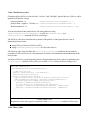
2.1.2.3 User initialization classes and user action classes
Geant4 has two types of user defined classes, called user initialization classes and user action classes.
User initialization classes are to be used for the initialization of your Geant4 application, while user
action classes are to be used during run processing. User initialization classes can be assigned to
G4RunManager by invoking the SetUserInitialization() method, whereas, the user action classes
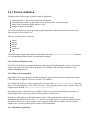
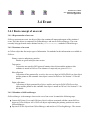
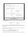
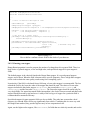
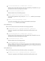
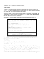
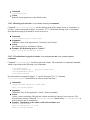
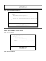
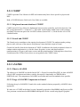
can be set via the SetUserAction() method. Source listing 2.1 shows the simplest example of main().
#include "G4RunManager.hh"
#include "G4UImanager.hh"
#include "ExN01DetectorConstruction.hh"
#include "ExN01PhysicsList.hh"
#include "ExN01PrimaryGeneratorAction.hh"
int main()
{
// construct the default run manager
G4RunManager* runManager = new G4RunManager;
// set mandatory initialization classes
runManager->SetUserInitialization(new ExN01DetectorConstruction);
runManager->SetUserInitialization(new ExN01PhysicsList);
// set mandatory user action class
runManager->SetUserAction(new ExN01PrimaryGeneratorAction);
// initialize G4 kernel
runManager->initialize();
// get the pointer to the UI manager and set verbosities
G4UImanager* UI = G4UImanager::getUIpointer();
UI->applyCommand("/run/verbose 1");
UI->applyCommand("/event/verbose 1");
UI->applyCommand("/tracking/verbose 1");
// start a run
int numberOfEvent = 3;
runManager->beamOn(numberOfEvent);
// job termination
delete runManager;
return 0;
}
Source listing 2.1.1
The simplest example of main().
2.1.3 Mandatory user classes
There are three classes which must be defined by the user. Two of them are user initialization classes,
and the other is the user action class. The base classes of these mandatory classes are abstract, and
Geant4 does not provide default behavior for them. G4RunManager checks the existence of these
mandatory classes when the initialize() and beamOn() methods are invoked. You must inherit from
the abstract base classes provided by Geant4 and derive your own classes.
2.1.3.1 G4VUserDetectorConstruction
The complete detector setup should be described in this class. The detector setup can be:
materials used in the detector,
geometry of the detector,
definition of the sensitivities,
and readout schemes.
Details of how to define materials and geometry will be given in sections following. Sensitivity
definition and readout schemes will be described in the next chapter.
2.1.3.2 G4VuserPhysicsList
In this class, you must specify all particles and physics processes which will be used in your simulation.
Also, cutoff parameters should be defined in this class.
2.1.3.3 G4VuserPrimaryGeneratorAction
The way of generating a primary event should be given in this class. This class has a public virtual
method named generatePrimaries(). This method will be invoked at the beginning of each event.
Details will be given in Section 2.6. Please note that Geant4 does not provide any default behavior for
generating a primary event.
2.1.4. Optional user action classes
Geant4 provides five user hook classes:
G4UserRunAction
G4UserEventAction
G4UserStackingAction
G4UserTrackingAction
G4UserSteppingAction
There are several virtual methods in each class, and you can specify additional procedures at every
important place in your simulation application. Details on each class will be given in Section 3.18.
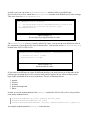
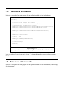
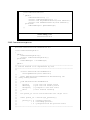
2.1.5. G4UImanager and UI command submission
Geant4 provides a category named intercoms. G4UImanager is the manager class of this category.
Using the functionalities of this category, you can invoke set methods of class objects of which you do
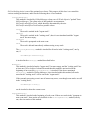
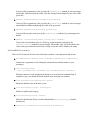
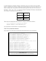
not know the pointer. In Source listing 2.1.1, the verbosities of various Geant4 manager classes are set.
Detailed mechanism description and usage of intercoms will be given in the next chapter, with a list of
available commands. Command submission can be done all through the application.
#include "G4RunManager.hh"
#include "G4UImanager.hh"
#include "G4UIterminal.hh"
#include
#include
#include
#include
#include
#include
#include
"N02VisManager.hh"
"N02DetectorConstruction.hh"
"N02PhysicsList.hh"
"N02PrimaryGeneratorAction.hh"
"N02RunAction.hh"
"N02EventAction.hh"
"N02SteppingAction.hh"
#include "g4templates.hh"
int main(int argc,char** argv)
{
// construct the default run manager
G4RunManager * runManager = new G4RunManager;
// set mandatory initialization classes
N02DetectorConstruction* detector = new N02DetectorConstruction;
runManager->SetUserInitialization(detector);
runManager->SetUserInitialization(new N02PhysicsList);
// visualization manager
G4VisManager* visManager = new N02VisManager;
visManager->initialize();
// set user action classes
runManager->SetUserAction(new
runManager->SetUserAction(new
runManager->SetUserAction(new
runManager->SetUserAction(new
N02PrimaryGeneratorAction(detector));
N02RunAction);
N02EventAction);
N02SteppingAction);
// get the pointer to the User Interface manager
G4UImanager* UI = G4UImanager::getUIpointer();
if(argc==1)
// Define (G)UI terminal for interactive mode
{
G4UIsession * session = new G4UIterminal;
UI->applyCommand("/control/execute prerun.g4mac");
session->sessionStart();
delete session;
}
else
// Batch mode
{
G4String command = "/control/execute ";
G4String fileName = argv[1];
UI->applyCommand(command+fileName);
}
// job termination
delete visManager;
delete runManager;
return 0;
}
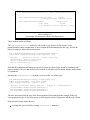
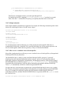
Source list 2.1.2
An example of main() using interactive terminal and visualization.
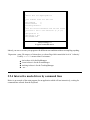
2.1.6 G4cout and G4cerr
G4cout and G4cerr are iostream objects defined by Geant4. The usage of these objects in your codes is
exactly the same as the ordinary cout and cerr, but the output streams will be handled by G4UImanager.
Thus, you can display output strings into another window, or store them into a file. Manipulation of
these output streams will be described in Section 3.15. You are advised to use these objects instead of
the ordinary cout and cerr.
About the authors
Geant4 User’s Guide
For Application Developers
Getting started with Geant4
2.2 How to define a detector geometry
2.2.1 Basic concepts
A detector geometry in Geant4 is made of a number of volumes. The largest volume is called the World
volume. It must contain all other volumes in the detector geometry. The other volumes are created and
placed inside previous volumes, included in the World volume.
Each volume is created by describing its shape and its physical characteristics, and then placing it inside
a containing volume.
When a volume is placed within another volume, we call the former volume the daughter volume and
the latter the mother volume. The coordinate system used to specify where the daughter volume is
placed, is the coordinate system of the mother volume.
To describe a volume’s shape, we use the concept of a solid. A solid is a geometrical object that has a
shape and specific values for each of that shape’s dimensions. A cube with a side of 10 centimeters and
a cylinder of radius 30 cm and length 75 cm are examples of solids.
To describe a volume’s full properties, we use a logical volume. It includes the geometrical properties of
the solid, and adds physical characteristics: the material of the volume; whether it contains any sensitive
detector elements; the magnetic field; etc.
We have yet to describe how to position the volume. To do this you create a physical volume, which
places a copy of the logical volume inside a larger, containing, volume.
2.2.2 Create a simple volume
What do you need to do to create a volume?
Create a solid.
Create a logical volume, using this solid, and adding other attributes.
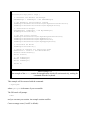
2.2.3 Choose a solid
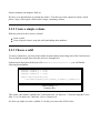
To create a simple box, you only need to define its name and its extent along each of the Cartesian axes.
You can find an example how to do this in Novice Example N01.
In the detector description in the source file ExN01DetectorConstruction.cc, you will find the
following box definition:
G4double expHall_x = 3.0*m;
G4double expHall_y = 1.0*m;
G4double expHall_z = 1.0*m;
G4Box* experimentalHall_box
= new G4Box("expHall_box",expHall_x,expHall_y,expHall_z);
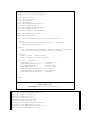
Source listing 2.2.1
Creating a box.
This creates a box named "expHall_box" with extent from -3.0 meters to +3.0 meters along the X axis,
from -1.0 to 1.0 meters in Y, and from -1.0 to 1.0 meters in Z.
It is also very simple to create a cylinder. To do this, you can use the G4Tubs class.
G4double
G4double
G4double
G4double
G4double
innerRadiusOfTheTube = 0.*cm;
outerRadiusOfTheTube = 60.*cm;
hightOfTheTube = 50.*cm;
startAngleOfTheTube = 0.*deg;
spanningAngleOfTheTube = 360.*deg;
G4Tubs* tracker_tube
= new G4Tubs("tracker_tube",
innerRadiusOfTheTube,
outerRadiusOfTheTube,
hightOfTheTube,
startAngleOfTheTube,
spanningAngleOfTheTube);
Source listing 2.2.2
Creating a cylinder.
This creates a full cylinder, named "tracker_tube", of radius 60 centimeters and length 50 cm.
2.2.4 Create a logical volume
To create a logical volume, you must start with a solid and a material. So, using the box created above,
you can create a simple logical volume filled with argon gas (see materials) by entering:
G4LogicalVolume* experimentalHall_log
= new G4LogicalVolume(experimentalHall_box,Ar,"expHall_log");
This logical volume is named "expHall_log".
Similarly we create a logical volume with the cylindrical solid filled with aluminium
G4LogicalVolume* tracker_log
= new G4LogicalVolume(tracker_tube,Al,"tracker_log");
and named "tracker_log"
2.2.5 Place a volume
How do you place a volume? You start with a logical volume, and then you decide the already existing
volume inside of which to place it. Then you decide where to place its center within that volume, and
how to rotate it. Once you have made these decisions, you can create a physical volume, which is the
placed instance of the volume, and embodies all of these atributes.
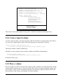
2.2.6 Create a physical volume
You create a physical volume starting with your logical volume. A physical volume is simply a placed
instance of the logical volume. This instance must be placed inside a mother logical volume. For
simplicity it is unrotated:
G4double trackerPos_x = -1.0*meter;
G4double trackerPos_y = 0.0*meter;
G4double trackerPos_z = 0.0*meter;
G4VPhysicalVolume* tracker_phys
= new G4PVPlacement(0,
// no rotation
G4ThreeVector(trackerPos_x,trackerPos_y,trackerPos_z),
// translation position
tracker_log,
// its logical volume
"tracker",
// its name
experimentalHall_log,
// its mother (logical) volume
false,
// no boolean operations
0);
// its copy number
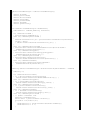
Source listing 2.2.3
A simple physical volume.
This places the logical volume tracker_log at the origin of the mother volume
experimentalHall_log, unrotated. The resulting physical volume is named "tracker" and has a copy
number of 0.
An exception exists to the rule that a physical volume must be placed inside a mother volume. That
exception is for the World volume, which is the largest volume created, and which contains all other
volumes. This volume obviously cannot be contained in any other. Instead, it must be created as a
G4PVPlacement with a null mother pointer. It also must be unrotated, and it must be placed at the origin
of the global coordinate system.
Generally, it is best to choose a simple solid as the World volume, and in Example N01, we use the
experimental hall:
G4VPhysicalVolume* experimentalHall_phys
= new G4PVPlacement(0,
G4ThreeVector(0.,0.,0.),
experimentalHall_log,
"expHall",
0,
false,
0);
//
//
//
//
//
//
//
Source listing 2.2.4
The World volume from Example N01.
no rotation
translation position
its logical volume
its name
its mother volume
no boolean operations
its copy number
2.2.7 Coordinate systems and rotations
In Geant4, the rotation matrix associated to a placed physical volume represents the rotation of the
reference system of this volume with respect to its mother.
A rotation matrix is normally constructed as in CLHEP, by instantiating the identity matrix and then
applying a rotation to it. This is also demonstrated in Example N04.
About the authors
Geant4 User’s Guide
For Application Developers
Getting started with Geant4
2.3 How to specify material in the detector
2.3.1 General considerations
In nature, general materials (chemical compounds, mixtures) are made of elements, and elements are
made of isotopes. Therefore, these are the three main classes designed in Geant4. Each of these classes
has a table as a static data member, which is for keeping track of the instances created of the respective
classes.
The G4Element class describes the properties of the atoms:
atomic number,
number of nucleons,
atomic mass,
shell energy,
as well as quantities such as cross sections per atom, etc.
The G4Material class describes the macroscopic properties of matter:
density,
state,
temperature,
pressure,
as well as macroscopic quantities like radiation length, mean free path, dE/dx, etc.
The G4Material class is the one which is visible to the rest of the toolkit, and is used by the tracking, the
geometry, and the physics. It contains all the information relative to the eventual elements and isotopes
of which it is made, at the same time hiding the implementation details.
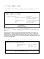
2.3.2 Define a simple material
In the example below, liquid argon is created, by specifying its name, density, mass per mole, and
atomic number.
G4double density = 1.390*g/cm3;
G4double a = 39.95*g/mole;
G4Material* lAr = new G4Material(name="liquidArgon", z=18., a, density);
Source listing 2.3.1
Creating liquid argon.
The pointer to the material, lAr, will be used to specify the matter of which a given logical volume is
made:
G4LogicalVolume* myLbox = new G4LogicalVolume(aBox,lAr,"Lbox",0,0,0);
2.3.3 Define a molecule
In the example below, the water, H2O, is built from its components, by specifying the number of atoms
in the molecule.
a = 1.01*g/mole;
G4Element* elH = new G4Element(name="Hydrogen",symbol="H" , z= 1., a);
a = 16.00*g/mole;
G4Element* elO = new G4Element(name="Oxygen"
,symbol="O" , z= 8., a);
density = 1.000*g/cm3;
G4Material* H2O = new G4Material(name="Water",density,ncomponents=2);
H2O->AddElement(elH, natoms=2);
H2O->AddElement(elO, natoms=1);
Source listing 2.3.2
Creating water by defining its molecular components.
2.3.4 Define a mixture by fractional mass
In the example below, air is built from nitrogen and oxygen, by giving the fractional mass of each
component.
a = 14.01*g/mole;
G4Element* elN = new G4Element(name="Nitrogen",symbol="N" , z= 7., a);
a = 16.00*g/mole;
G4Element* elO = new G4Element(name="Oxygen"
,symbol="O" , z= 8., a);
density = 1.290*mg/cm3;
G4Material* Air = new G4Material(name="Air ",density,ncomponents=2);
Air->AddElement(elN, fractionmass=70*perCent);
Air->AddElement(elO, fractionmass=30*perCent);
Source listing 2.3.3
Creating air by defining the fractional mass of its components.
2.3.5 Print material information
G4cout << H2O;
G4cout << *(G4Material::GetMaterialTable());
\\ print a given material
\\ print the list of materials
Source listing 2.3.4
Printing information about materials.
In examples/novice/N03/N03DetectorConstruction.cc, you will find examples of all possible ways
to build a material.
About the authors
Geant4 User’s Guide
For Application Developers
Getting started with Geant4
2.4 How to specify a particle
2.4.1 Particle definition
Geant4 provides various types of particles used in simulations:
ordinary particles, such as electron, proton, and gamma
resonant particles with very short life, such as vector mesons, and delta baryons
nuclei, such as deuteron, alpha, and heavy ions
quarks, di-quarks, and gluons
The G4ParticleDefinition class is provided to represent particles, and each particle has its own class
derived from G4ParticleDefinition.
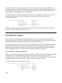
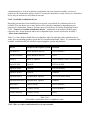
There are 6 major particle categories:
lepton
meson
baryon
boson
shortlived
ion
Particles in these categories are defined in sub-directories under geant4/source/particles, and there
is a corresponding granular library for each particle category.
2.4.1.1 G4ParticleDefinition class
The G4ParticleDefinition class has properties to characterize individual particles, such as, name, mass,
charge, spin, and so on. Most of these properties are "read-only" and can not be changed by users
without rebuilding libraries.
2.4.1.2 How to access a particle
Each particle class type represents an individual particle type, and each class has a single static object.
(There are some exceptions. Please see Section 3.9 for details.)
For example, the G4Electron class represents the "electron" and G4Electron::theElectron is the only
object, a so-called singleton, of the G4Electron class. You can get the pointer to this "electron" object by
using the static method G4Electron::ElectronDefinition().
More than 100 types of particles are provided by default, to be used in various physics processes. In
normal applications, users do not need to define particles for themselves.
Particles are static objects of individual particle classes. This means that these objects will be
instantiated automatically before the main() routine is executed. However, you must explicitly declare
the particle classes you want somewhere in your program, otherwise the compiler can not recognize
which classes you need, and no particle classes will be instantiated.
2.4.1.3 Dictionary of particles
The G4ParticleTable class is provided as a dictionary of particles. Various utility methods are provided,
such as:
FindParticle(G4String name):
find the particle by name
FindParticle(G4int PDGencoding): find the particle by PDG encoding
G4ParticleTable is also defined as a singleton object, and the static method
G4ParticleTable::GetParticleTable() gives you its pointer.
Particles are registered automatically in construction. You do not need (and can not) execute registration
by yourself.
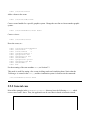
2.4.2 Cuts
The G4ParticleDefinition class has a single cut value in range of the production threshold. By using the
SetCuts() method of each particle class, this cut-off value in range should be converted to the cut-off
energies for all materials defined in the geometry. You can get the cut value in range by using the
GetLengthCuts() method and the threshold energy of a material by using the GetEnergyThreshold(
const G4Material* ) method. The details of "cut" are described in Section 3.18 of the "User’s
Guide".
2.4.3 Specify particles and physics processes
The G4VuserPhysicsList class is one of the base classes for the "user mandatory classes" (see Section
2.1), in which you have to specify all particles and physics processes which will be used in your
simulation. In addition, the cut-off parameter in range should be defined in this class.
A user must create his own class derived from G4VuserPhysicsList and implement the following pure
virtual methods:
ConstructParticle(): construction of particles
ConstructPhysics(): construct processes and register them to particles
SetCuts():
setting a cut value in range to all particles
In this section are some simple examples of the ConstructParticle() and SetCuts() methods. For
ConstructProcess() methods, please see Section 2.5.
2.4.3.1 Construct particles
The ConstructParticle() method is a pure virtual method, in which you should call the static member
functions for all the particles you want. This ensures that objects of these particles will be created as
explained in Section 2.4.1.
For example, suppose you need a proton and a geantino, which is a virtual particle used for simulation
and which does not interact with materials. The ConstructParticle() method is implemented as
below:
void ExN01PhysicsList::ConstructParticle()
{
G4Proton::ProtonDefinition();
G4Geantino::GeantinoDefinition();
}
Source listing 2.4.1
Construct a proton and a geantino.
The total number of particles pre-defined in Geant4 is more than 100, and it can be cumbersome to list
all particles by this method. Some utility classes can be used if you want all the particles of some Geant4
particle category. There are 6 classes provided which correspond to the 6 particle categories.
G4BosonConstructor
G4LeptonConstructor
G4MesonConstructor
G4BarionConstructor
G4IonConstructor
G4ShortlivedConstructor
You can see an example of this in ExN04PhysicsList, as listed below.
void ExN04PhysicsList::ConstructLeptons()
{
// Construct all leptons
G4LeptonConstructor pConstructor;
pConstructor.ConstructParticle();
}
Source listing 2.4.2
Construct all leptons.
2.4.3.2 Set the cuts
The SetCuts() method is a pure virtual method. You should set cut-off values for all particles by using
the SetCuts() method of each particle class. Construction of particles, geometry, and processes should
precede invocation of SetCuts(). G4RunManager takes care of usual applications.
This idea of a "unique cut value in range" is one of the important features of Geant4 used to handle cut
values in a coherent manner. For usual applications, users need to determine only one cut value in range,
and apply this value to all particles.
In such a case, you can use the SetCutsWithDefault() method, which is provided in the
G4VuserPhysicsList class, which has a defaultCutValue member as the default cut-off value in range.
This value is used in SetCutsWithDefault().
void ExN04PhysicsList::SetCuts()
{
//
the G4VUserPhysicsList::SetCutsWithDefault() method sets
//
the default cut value for all particle types
SetCutsWithDefault();
}
Source listing 2.4.3
Set cut values by using the default cut value.
The defaultCutValue is set to 1.0 mm by default. Of course, you can set the new default cut value in
the constructor of your physics list class as shown below. You can also use the SetDefaultCutValue()
method in the G4VUserPhysicsList.
ExN04PhysicsList::ExN04PhysicsList():
{
// default cut value (1.0mm)
defaultCutValue = 1.0*mm;
}
G4VUserPhysicsList()
Source listing 2.4.4
Set the default cut value.
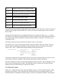
If you want to set different cut values for different particles, you need to be aware of the order of the
particle types in setting the cut vales, because some particles require the cut values of other particle
types in the calculation of the cross section tables. The rule of ordering follows:
1.
2.
3.
4.
5.
gamma
electron
positron
proton and antiproton
others
In order to ease the implementation of the SetCuts() method, the G4VuserPhysicsList class provides
some utility methods such as:
SetCutValue(G4double cut_value, G4String particle_name)
SetCutValueForOthers(G4double cut_value)
SetCutValueForOtherThan(G4double cut_value, G4ParticleDefinition* a_particle)
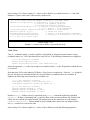
An example implementation of SetCuts() is shown below:
void ExN03PhysicsList::SetCuts()
{
// set cut values for gamma at first and for e- second and next for e+,
// because some processes for e+/e- need cut values for gamma
SetCutValue(cutForGamma, "gamma");
SetCutValue(cutForElectron, "e-");
SetCutValue(cutForElectron, "e+");
// set cut values for proton and anti_proton before all other hadrons
// because some processes for hadrons need cut values for proton/anti_proton
SetCutValue(cutForProton, "proton");
SetCutValue(cutForProton, "anti_proton");
SetCutValueForOthers(defaultCutValue);
}
Source listing 2.4.5
Example implementation of the SetCuts() method.
You should not change cut values inside the event loop. You can change cut values for run by run by
using the user command of /run/particle/SetCuts .
About the authors
Geant4 User’s Guide
For Application Developers
Getting started with Geant4
2.5 How to specify a physics process
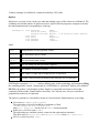
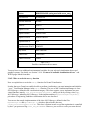
2.5.1 Physics processes
Physics processes describe how to interact with materials and particles. Various kinds of
electromagnetic, hadronic, and other interactions are provided in Geant4. There are 7 major process
categories:
electromagnetic
hadronic
transportation
decay
optical
photolepton_hadron
parameterisation
G4VProcess class is provided as a base class of physics processes. Every process describes its behavior
by using three (virtual) DoIt methods:
AtRestDoIt
AlongStepDoIt
PostStepDoIt
and three corresponding GetPhysicalInteractionLength methods. The details of these methods are
described in Section 3.11.
The following classes are used as base classes of simple processes:
G4VAtRestProcess
- processes with only AtRestDoIt
G4VContinuousProcess - processes with only AlongStepDoIt
G4VDiscreteProcess
- processes with only PostStepDoIt
And another 4 virtual classes, such as G4VContinuousDiscreteProcess, are provided for complex
processes.
2.5.2 Managing processes
The G4ProcessManager class contains a list of processes that a particle can undertake. It has
information on the order of invocation of the processes, as well as which kind of DoIt is valid for each
process in the list. A G4ProcessManager object corresponds to each particle and is attached to the
G4ParticleDefiniton class.
In order to validate processes, processes should be registered in the particle’s G4ProcessManager, with
ordering information included by using the AddProcess() and SetProcessOrdering() methods. For
registration of simple processes, the AddAtRestProcess(), AddContinuousProcess(), and
AddDiscreteProcess() methods can be used.
G4ProcessManager has the functionality to toggle on/off some processes during running time by using
the ActivateProcess() and InActivateProcess() methods. (Do not use these methods in the PreInit
phase. These methods are valid after the registration of the processes finishes.)
2.5.3 Specifying physics processes
The G4VUserPhysicsList class is the base class for a "user mandatory class" (see Section 2.1), in which
you have to specify all physics processes together with all particles which will be used in your
simulation. The user must create his own class derived from G4VuserPhysicsList and implement the
pure virtual method ConstructPhysics().
The G4VUserPhysicsList class creates and attaches G4ProcessManager objects to all particle classes
defined in the ConstructParticle() method.
2.5.3.1 Add a transportation method
The G4Transportation class (and/or related classes) should be registered to all particle classes, because
particles can not be tracked without a transportation process, which describe how to move in space and
time. The AddTransportation() method is provided in the G4VUserPhysicsList class, and it must be
called in the ConstructPhysics() method.
void G4VUserPhysicsList::AddTransportation()
{
// create G4Transportation
G4Transportation* theTransportationProcess = new G4Transportation();
// loop over all particles in G4ParticleTable and register the transportation process
theParticleIterator->reset();
while( (*theParticleIterator)() ){
G4ParticleDefinition* particle = theParticleIterator->value();
G4ProcessManager* pmanager = particle->GetProcessManager();
// adds transportation to all particles except shortlived particles
if (!particle->IsShortLived()) {
pmanager ->AddProcess(theTransportationProcess);
// set ordering to the first for AlongStepDoIt
pmanager ->SetProcessOrderingToFirst(theTransportationProcess, idxAlongStep);
}
}
}
Source listing 2.5.1
Add a transportation method.
2.5.3.2 Create and register physics processes
is a pure virtual method which is used to create physics processes and register
them to particles. For example, if you only use the G4Geantino class of particle, geantinos undertake the
transportation process only, and the ConstructProcess() method is implemented as below:
ConstructProcess()
void ExN01PhysicsList::ConstructProcess()
{
// Define transportation process
AddTransportation();
}
Source listing 2.5.2
Register processes for a geantino.
Registration of electromagnetic processes for the gamma is implemented as below:
void MyPhysicsList::ConstructProcess()
{
// Define transportation process
AddTransportation();
// electromagnetic processes
ConstructEM();
}
void MyPhysicsList::ConstructEM()
{
// Get the process manager for gamma
G4ParticleDefinition* particle = G4Gamma::GammaDefinition();
G4ProcessManager* pmanager = particle->GetProcessManager();
// Construct processes for gamma
G4PhotoElectricEffect * thePhotoElectricEffect = new G4PhotoElectricEffect();
G4ComptonScattering * theComptonScattering = new G4ComptonScattering();
G4GammaConversion* theGammaConversion = new G4GammaConversion();
// Register processes to gamma’s process manager
pmanager->AddDiscreteProcess(thePhotoElectricEffect);
pmanager->AddDiscreteProcess(theComptonScattering);
pmanager->AddDiscreteProcess(theGammaConversion);
}
Source listing 2.5.3
Register processes for a gamma.
Registration in G4ProcessManager is a complex procedure for other processes and particles, because
the relations between processes are crucial for some processes. Please see Section 3.10 and the example
codes.
About the authors
Geant4 User’s Guide
For Application Developers
Getting started with Geant4
2.6 How to generate a primary event
2.6.1 Generate primary events
G4VuserPrimaryGeneratorAction is one of the mandatory classes available for deriving your own
concrete class. In your concrete class, you have to specify how a primary event should be generated.
Actual generation of primary particles will be done by concrete classes of G4VPrimaryGenerator,
explained in the following sub-section. Your G4VUserPrimaryGeneratorAction concrete class just
arranges the way primary particles are generated.
#ifndef ExN01PrimaryGeneratorAction_h
#define ExN01PrimaryGeneratorAction_h 1
#include "G4VUserPrimaryGeneratorAction.hh"
class G4ParticleGun;
class G4Event;
class ExN01PrimaryGeneratorAction : public G4VUserPrimaryGeneratorAction
{
public:
ExN01PrimaryGeneratorAction();
~ExN01PrimaryGeneratorAction();
public:
void generatePrimaries(G4Event* anEvent);
private:
G4ParticleGun* particleGun;
};
#endif
#include
#include
#include
#include
#include
#include
"ExN01PrimaryGeneratorAction.hh"
"G4Event.hh"
"G4ParticleGun.hh"
"G4ThreeVector.hh"
"G4Geantino.hh"
"globals.hh"
ExN01PrimaryGeneratorAction::ExN01PrimaryGeneratorAction()
{
G4int n_particle = 1;
particleGun = new G4ParticleGun(n_particle);
particleGun->SetParticleDefinition(G4Geantino::GeantinoDefinition());
particleGun->SetParticleEnergy(1.0*GeV);
particleGun->SetParticlePosition(G4ThreeVector(-2.0*m,0.0*m,0.0*m));
}
ExN01PrimaryGeneratorAction::~ExN01PrimaryGeneratorAction()
{
delete particleGun;
}
void ExN01PrimaryGeneratorAction::generatePrimaries(G4Event* anEvent)
{
G4int i = anEvent->get_eventID() % 3;
switch(i)
{
case 0:
particleGun->SetParticleMomentumDirection(G4ThreeVector(1.0,0.0,0.0));
break;
case 1:
particleGun->SetParticleMomentumDirection(G4ThreeVector(1.0,0.1,0.0));
break;
case 2:
particleGun->SetParticleMomentumDirection(G4ThreeVector(1.0,0.0,0.1));
break;
}
particleGun->generatePrimaryVertex(anEvent);
}
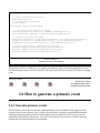
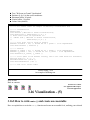
Source listing 2.6.1
An example of a G4VUserPrimaryGeneratorAction concrete class using G4ParticleGun.
2.6.1.1 Selection of the generator
In the constructor of your G4VUserPrimaryGeneratorAction, you should instantiate the primary
generator(s). If necessary, you need to set some initial conditions for the generator(s).
In Source listing 2.6.1, G4ParticleGun is constructed to use as the actual primary particle generator.
Methods of G4ParticleGun are described in the following section. Please note that the primary generator
object(s) you construct in your G4VUserPrimaryGeneratorAction concrete class must be deleted in your
destructor.
2.6.1.2 Generation of an event
G4VUserPrimaryGeneratorAction has a pure virtual method named generatePrimaries(). This
method is invoked at the beginning of each event. In this method, you have to invoke the
G4VPrimaryGenerator concrete class you instantiated via the generatePrimaryVertex() method.
You can invoke more than one generator and/or invoke one generator more than once. Mixing up
several generators can produce a more complicated primary event.
2.6.2 G4VPrimaryGenerator
Geant4 provides a couple of G4VPrimaryGenerator concrete classes. One is G4ParticleGun and the
other is G4HEPEvtInterface. The former is explained in this sub-section, whereas the latter will be
discussed in Section 3.5.
2.6.2.1 G4ParticleGun
G4ParticleGun is a generator provided by Geant4. This class generates primary particle(s) with given
momentum and position. This class does not provide any sort of randomizing.
It is a rather frequent user requirement to generate a primary with randomized energy, momentum,
and/or position. Such randomization can be realized by invoking various set methods provided by
G4ParticleGun. Invokation of these methods should be implemented in the generatePrimaries()
method of your concrete G4VUserPrimaryGeneratorAction class, before invoking
generatePrimaryVertex() of G4ParticleGun. Geant4 provides various random number generation
methods with various distributions (see Section 3.17).
2.6.2.2 Public methods of G4ParticleGun
The following methods are provided by G4ParticleGun, and all of them can be invoked from the
generatePrimaries() method in your concrete G4VUserPrimaryGeneratorAction class.
void
void
void
void
void
void
void
void
SetParticleDefinition(G4ParticleDefinition*)
SetParticleMomentum(G4ParticleMomentum)
SetParticleMomentumDirection(G4ThreeVector)
SetParticleEnergy(G4double)
SetParticleTime(G4double)
SetParticlePosition(G4ThreeVector)
SetParticlePolarization(G4ThreeVector)
SetNumberOfParticles(G4int)
About the authors
Geant4 User’s Guide
For Application Developers
Getting started with Geant4
2.7 How to make an executable program
2.7.1 Building ExampleN01 in a unix environment
The code for the user examples in Geant4 is placed in the directory $G4INSTALL/examples, where
$G4INSTALL is the environment variable set to the place where the Geant4 distribution is installed (set
by default to $HOME/geant4). In the following sections, a quick overview on how the GNUmake
mechanism works in Geant4 will be given, and we will show how to build a concrete example,
"ExampleN01", which is part of the Geant4 distribution.
2.7.1.1 How GNUmake works in Geant4
The GNUmake process in Geant4 is mainly controlled by the following GNUmake script files
(*.gmk scripts are placed in $G4INSTALL/config):
architecture.gmk invoking and defining all the architecture specific settings and paths which are
stored in $G4INSTALL/config/sys.
common.gmk
defining all general GNUmake rules for building objects and libraries
globlib.gmk
defining all general GNUmake rules for building compound libraries
binmake.gmk
defining the general GNUmake rules for building executables
GNUmakefile
placed inside each directory in the Geant4 distribution and defining directives
specific to build a library, a set of sub-libraries, or an executable.
Kernel libraries are placed by default in $G4INSTALL/lib/$G4SYSTEM, where $G4SYSTEM specifies the
system architecture and compiler in use. Executable binaries are placed in
$G4WORKDIR/bin/$G4SYSTEM, and temporary files (object-files and data products of the compilation
process) in $G4WORKDIR/tmp/$G4SYSTEM. $G4WORKDIR (set by default to $G4INSTALL) should be set by
the user to specify the place his/her own workdir for Geant4 in the user area.
For more information on how to build Geant4 kernel libraries and set up the correct environment for
Geant4, refer to the "Installation Guide".
2.7.1.2 Building the executable
The compilation process to build an executable, such as an example from $G4INSTALL/examples, is
started by invoking the "gmake" command from the (sub)directory in which you are interested. To build,
for instance, exampleN01 in your $G4WORKDIR area, you should copy the module
$G4INSTALL/examples to your $G4WORKDIR and do the following actions:
> cd $G4WORKDIR/examples/novice/N01
> gmake
This will create, in $G4WORKDIR/bin/$G4SYSTEM, the "exampleN01" executable, which you can invoke
and run. You should actually add $G4WORKDIR/bin/$G4SYSTEM to $PATH in your environment.
2.7.2 Building ExampleN01 in a Windows Environment
The procedure to build a Geant4 executable on a system based on OS Windows/95-98 or Windows/NT
is similar to what should be done on a UNIX based system, assuming that your system is equipped with
GNUmake, MS-Visual C++ compiler and the required software to run Geant4 (see "Installation Guide").
2.7.2.1 Building the executable
See paragraph 2.7.1.
About the authors
Geant4 User’s Guide
For Application Developers
Getting started with Geant4
2.8 How to specify a user interface
2.8.1 Introduction
The direct use of Geant4 classes in a C++ program offers a first ground level of interactivity. To avoid
too much programming, a command interpreter has been introduced, the intercoms category. This
second level of interactivity permits the steering of a simulation by execution of commands.
The capturing of commands is handled by a C++ abstract intercoms class, G4UIsession. This interface
method opens an important door towards various user interface tools, like Motif.
The interfaces category realizes some implementation of command "capturer". The richness of the
collaboration has permitted different groups to offer various front-ends to the Geant4 command system.
We list below, according their main technological choices, the various command handler
implementations:
batch
M.Asai
Read and execute a file containing Geant4 commands.
terminal
M.Asai
Command capture and dump of responses is done by using cin/cout.
Xm, Xaw, Win32 G.Barrand
Variations of the upper one by using a Motif, Athena or Windows widget to retreive
commands.
GAG
M.Nagamatu
Geant4 Adaptive GUI. Java and Tcl/Tk versions are available.
See http://erpc1.naruto-u.ac.jp/~geant4
OPACS
G.Barrand
An OPACS/Wo widget manager implementation.
See http://www.lal.in2p3.fr/OPACS: working with Geant4.
XVT
G.Cosmo
A client/server solution. The front-end is build with the XVT interface builder.
2.8.2 How to use a given interface
To use a given interface (G4UIxxx, where xxx = terminal, Xm, Xaw, Win32, GAG, Wo, XVT, ...)
someone has:
to build the Geant4/interfaces library with the C++ preprocessor macro
G4UI_BUILD_xxx_SESSION set,
to include in its main program the line:
#include
to include the following code :
G4UIsession* session = new G4UIxxx;
session->SessionStart();
to compile its main program with the C++ preprocessor macro G4UI_USE_xxx set.
to link with the proper library (Motif,...).
See an example with G4UIterminal in "How to execute a program".
2.8.3 G4UIXm, G4UIXaw, G4UIWin32 interfaces
These interfaces are versions of G4UIterminal implemented over libraries like Motif, Athena and
WIN32. G4UIXm uses the Motif XmCommand widget to capture command. G4UIXaw uses the Athena
dialog widget, and G4UIWin32 uses the Windows "edit" component to do the command capturing. The
commands "exit, cont, help, ls, cd..." are also supported.
These interfaces are usefull if working in conjunction with visualization drivers that use the Xt library or
the WIN32 one.
The usage of these interfaces, as explained in Section 2.8.2, are driven by the C++ preprocessor macros:
G4UI_BUILD_XM_SESSION, G4UI_USE_XM
G4UI_BUILD_XAW_SESSION, G4UI_USE_XAW
G4UI_BUILD_WIN32_SESSION, G4UI_USE_WIN32
About the authors
Geant4 User’s Guide
For Application Developers
Getting started with Geant4
2.9 How to execute your program
2.9.1 Introduction
A Geant4 application can be run either in
‘purely hard-coded‘ batch mode
batch mode, but reading a macro of commands
interactive mode, driven by command lines
interactive mode via a Graphical User Interface
The last mode will be covered in Section 2.10. The first three modes are explained here.
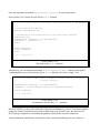
2.9.2 ’Hard-coded’ batch mode
Below is an example of the main program for an application which will run in batch mode.
int main()
{
// Construct the default run manager
G4RunManager* runManager = new G4RunManager;
// set mandatory initialization classes
runManager->SetUserInitialization(new ExN01DetectorConstruction);
runManager->SetUserInitialization(new ExN01PhysicsList);
// set mandatory user action class
runManager->SetUserAction(new ExN01PrimaryGeneratorAction);
// Initialize G4 kernel
runManager->Initialize();
// start a run
int numberOfEvent = 1000;
runManager->BeamOn(numberOfEvent);
// job termination
delete runManager;
return 0;
}
Source listing 2.9.1
An example of the main() routine for an application which will run in batch mode.
Even the number of events in the run is ‘frozen‘. To change this number you must at least recompile
main().
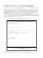
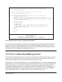
2.9.3 Batch mode with macro file
Below is an example of the main program for an application which will run in batch mode, but reading a
file of commands.
int main(int argc,char** argv) {
// Construct the default run manager
G4RunManager * runManager = new G4RunManager;
// set mandatory initialization classes
runManager->SetUserInitialization(new MyDetectorConstruction);
runManager->SetUserInitialization(new MyPhysicsList);
// set mandatory user action class
runManager->SetUserAction(new MyPrimaryGeneratorAction);
// Initialize G4 kernel
runManager->Initialize();
//read a macro file of commands
G4UImanager * UI = G4UImanager::getUIpointer();
G4String command = "/control/execute ";
G4String fileName = argv[1];
UI->applyCommand(command+fileName);
delete runManager;
return 0;
}
Source listing 2.9.2
An example of the main() routine for an application which will run in batch mode, but reading a
file of commands.
This example will be executed with the command:
> myProgram
run1.mac
where myProgram is the name of your executable and run1.mac is a macro of commands located in the
current directory, which could look like:
#
# Macro file for "myProgram.cc"
#
# set verbose level for this run
#
/run/verbose
2
/event/verbose
0
/tracking/verbose 1
#
# Set the initial kinematic and run 100 events
# electron 1 GeV to the direction (1.,0.,0.)
#
/gun/particle e/gun/energy 1 GeV
/run/beamOn 100
Source listing 2.9.3
A typical command macro.
Indeed, you can re-execute your program with different run conditions without recompiling anything.
Digression: many G4 category of classes have a verbose flag which controls the level of ’verbosity’.
Usually verbose=0 means silent. For instance
/run/verbose is for the RunManager
/event/verbose is for the EventManager
/tracking/verbose is for the TrackingManager
...etc...
2.9.4 Interactive mode driven by command lines
Below is an example of the main program for an application which will run interactively, waiting for
command lines entered from the keyboard.
int main(int argc,char** argv) {
// Construct the default run manager
G4RunManager * runManager = new G4RunManager;
// set mandatory initialization classes
runManager->SetUserInitialization(new MyDetectorConstruction);
runManager->SetUserInitialization(new MyPhysicsList);
// visualization manager
G4VisManager* visManager = new MyVisManager;
visManager->Initialize();
// set user action classes
runManager->SetUserAction(new
runManager->SetUserAction(new
runManager->SetUserAction(new
runManager->SetUserAction(new
MyPrimaryGeneratorAction);
MyRunAction);
MyEventAction);
MySteppingAction);
// Initialize G4 kernel
runManager->Initialize();
// Define UI terminal for interactive mode
G4UIsession * session = new G4UIterminal;
session->SessionStart();
delete session;
// job termination
delete visManager;
delete runManager;
return 0;
}
Source listing 2.9.4
An example of the main() routine for an application which will run interactively, waiting for
commands from the keyboard.
This example will be executed with the command:
> myProgram
where myProgram is the name of your executable.
The G4 kernel will prompt:
Idle>
and you can start your session. An example session could be:
Create an empty scene ("world" is default):
Idle> /vis/scene/create
Add a volume to the scene:
Idle> /vis/scene/add/volume
Create a scene handler for a specific graphics system. Change the next line to choose another graphic
system:
Idle> /vis/sceneHandler/create OGLIX
Create a viewer:
Idle> /vis/viewer/create
Draw the scene, etc.:
Idle>
Idle>
Idle>
Idle>
Idle>
Idle>
Idle>
Idle>
Idle>
Idle>
Idle>
/vis/scene/notifyHandlers
/run/verbose
0
/event/verbose
0
/tracking/verbose 1
/gun/particle mu+
/gun/energy 10 GeV
/run/beamOn 1
/gun/particle proton
/gun/energy 100 MeV
/run/beamOn 3
exit
For the meaning of the state machine Idle, see Section 3.3.
This mode is useful for runing a few events in debug mode and visualizing them. Notice that the
VisManager is created in the main(), and the visualization system is choosen via the command:
/vis/sceneHandler/create OGLIX
2.9.5 General case
Most of the examples in the $G4INSTALL/examples/ directory have the following main(), which
covers cases 2 and 3 above. Thus, the application can be run either in batch or interactive mode.
int main(int argc,char** argv) {
// Construct the default run manager
G4RunManager * runManager = new G4RunManager;
// set mandatory initialization classes
N03DetectorConstruction* detector = new N03DetectorConstruction;
runManager->SetUserInitialization(detector);
runManager->SetUserInitialization(new N03PhysicsList);
#ifdef G4VIS_USE
// visualization manager
G4VisManager* visManager = new N03VisManager;
visManager->Initialize();
#endif
// set user action classes
runManager->SetUserAction(new
runManager->SetUserAction(new
runManager->SetUserAction(new
runManager->SetUserAction(new
N03PrimaryGeneratorAction(detector));
N03RunAction);
N03EventAction);
N03SteppingAction);
// get the pointer to the User Interface manager
G4UImanager* UI = G4UImanager::GetUIpointer();
if (argc==1)
// Define UI terminal for interactive mode
{
G4UIsession * session = new G4UIterminal;
UI->ApplyCommand("/control/execute prerunN03.mac");
session->SessionStart();
delete session;
}
else
// Batch mode
{
G4String command = "/control/execute ";
G4String fileName = argv[1];
UI->ApplyCommand(command+fileName);
}
// job termination
#ifdef G4VIS_USE
delete visManager;
#endif
delete runManager;
return 0;
}
Source listing 2.9.5
The typical main() routine from the examples directory.
Notice that the visualization system is under the control of the precompiler variable G4VIS_USE. Notice
also that, in interactive mode, few intializations have been put in the macro prerunN03.mac which is
executed before the session start.
# Macro file for the initialization phase of "exampleN03.cc"
#
# Sets some default verbose flags
# and initializes the graphics.
#
/control/verbose 2
/control/saveHistory
/run/verbose 2
#
/run/particle/dumpCutValues
#
# Create empty scene ("world" is default)
/vis/scene/create
#
# Add volume to scene
/vis/scene/add/volume
#
# Create a scene handler for a specific graphics system
# Edit the next line(s) to choose another graphic system
#
#/vis/sceneHandler/create DAWNFILE
/vis/sceneHandler/create OGLIX
#
# Create a viewer
/vis/viewer/create
#
# Draw scene
/vis/scene/notifyHandlers
#
# for drawing the tracks
# if too many tracks cause core dump => storeTrajectory 0
/tracking/storeTrajectory 1
#/vis/scene/include/trajectories
Source listing 2.9.6
The prerunN03.mac macro.
Also, this example demonstrates that you can read and execute a macro interactively:
Idle> /control/execute
mySubMacro.mac
About the authors
Geant4 User’s Guide
For Application Developers
Getting started with Geant4
2.10 How to visualize the detector and events
2.10.1 Introduction
This section briefly explains how to perform Geant4 Visualization. The description here is based on the
sample program examples/novice/N03. More details are described in Section 3.16 "Visualization" and
Section 4.3 "More about visualization". See macro files
examples/novice/N03/visTutor/exN03VisX.mac, too.
2.10.2 Visualization drivers
Geant4 visualization is required to respond to a variety of user requirements. It is difficult to respond to
all of these with only one built-in visualizer, therefore Geant4 visualization defines an abstract interface
to any number of graphics systems. Here, a "graphics system" means either an application running as a
process independent of Geant4, or a graphics library compiled with Geant4. The Geant4 visualization
distribution supports concrete interfaces to several graphics systems, which are in many respects
complementary to each other. A concrete interface to a graphics system is called a "visualization driver".
You need not use all visualization drivers. You can select those suitable to your purposes. In the
following, for simplicity, we assume that the Geant4 libraries are built with the "DAWNFILE driver"
and the "OpenGL-Xlib driver" incorporated.
Notes for installing visualization drivers in building Geant4 libraries:
In order to perform Geant4 visualization, you have to build the Geant4 libraries with your selected
visualization drivers incorporated beforehand. The selection of visualization drivers can be done by
setting the proper C-pre-processor flags either manually or by using the GNUmakefile provided.
Each visualization driver has its own C-pre-processor flag. For example, the DAWNFILE driver is
incorporated by setting a flag G4VIS_BUILD_DAWNFILE_DRIVER to "1". Besides, there is a global
C-pre-processor flag G4VIS_BUILD, which must be set to "1", if you want to incorporate at least one
visualization driver.
The GNUmakefile config/G4VIS_BUILD.gmk, included in most of the provided GNUmakefiles, can set
proper C-pre-processor flags AUTOMATICALLY. All you have to do is to set environmental variables
for your selected visualization drivers. Each environmental variable has the same name as the
C-pre-processor flag of the corresponding visualization driver. The global flag G4VIS_BUILD is
automatically set if necessary. Below we assume that you follow this automatic way. (You can also set
the C-pre-processor flags with other strategies, if you want.)
In building Geant4 libraries, you can incorporate your selected visualization drivers by setting
environmental variables of the form G4VIS_BUILD_DRIVERNAME_DRIVER to "1", where the string
"DRIVERNAME" is a name of a selected visualization driver. Candidates for the names are listed in
Section 3.16.5.2 "How to use visualization drivers in an executable". See also the file
source/visualization/README.
For example, if you want to incorporate the DAWNFILE driver and the OpenGL-Xlib driver into the
Geant4 libraries under the UNIX C-shell environment, set environmental variables as follows before
building the libraries:
% setenv G4VIS_BUILD_DAWNFILE_DRIVER 1
% setenv G4VIS_BUILD_OPENGLX_DRIVER 1
2.10.3 How to realize visualization drivers in an executable
You can realize (use) visualization driver(s) you want in your Geant4 executable. These can only be
from the set installed in the Geant4 libraries. You will be warned if the one you request is not available.
In the standard distribution, each visualization driver can easily be realized as follows.
In the examples you will find user visualization managers, e.g.,
example/novice/N03/include/ExN03VisManager.hh and src/ExN03VisManager.cc. If you adopt
this style all you need to do is set the proper C-pre-processor flags either manually or by using the
GNUmakefile provided.
Each visualization driver has its own C-pre-processor flag. For example, the DAWNFILE driver is
incorporated by setting a flag G4VIS_USE_DAWNFILE to "1". Besides there is a global C-pre-processor
flag G4VIS_USE, which must be set to "1" if you want to realize at least one visualization driver in your
Geant4 executable.
The GNUmakefile config/G4VIS_USE.gmk, included in, e.g., example/novice/N03/GNUmakefile,
can set proper C-pre-processor flags AUTOMATICALLY. All you have to do is to set environmental
variables for visualization drivers you want to realize before compilation. Each environmental variable
has the same name as the C-pre-processor flag of the corresponding visualization driver. The global flag
G4VIS_USE is automatically set if necessary. Below we assume that you follow this automatic way. (You
can also set the C-pre-processor flags with other strategies, if you want.)
You can realize a visualization driver by setting an environmental variable, whose name has the form
G4VIS_USE_DRIVERNAME, to "1". Here, the string "DRIVERNAME" is the name of the visualization
driver. Candidates for the name are listed in Section 3.16.5.2 "How to use visualization drivers in an
executable". See also the file source/visualization/README.
For example, if you want to realize the DAWNFILE driver and the OpenGL-Xlib driver in your Geant4
executable under the UNIX C-shell environment, set environmental variables as follows before
compilation:
% setenv G4VIS_USE_DAWNFILE 1
% setenv G4VIS_USE_OPENGLX 1
The next section describes how to write your own visualization manager if you wish.
2.10.4 How to write the main() function for visualization
Now we explain how to write a visualization manager and the main() function for Geant4 visualization.
In order that your Geant4 executable is able to perform visualization, you must instantiate and initialize
your Visualization Manager in the main() function. The base class of the Visualization Manager is
G4VisManager, defined in the visualization category. This class requires you to implement one pure
virtual function, namely, void RegisterGraphicsSystems(), which you do by writing a class, e.g.,
ExN03VisManager, inheriting the class G4VisManager. In the implementation of
ExN03VisManager::RegisterGraphicsSystems(), procedures for registering candidate visualization
drivers are described. The class ExN03VisManager is written in such a way that registration is controlled
by the C-pre-processor flags G4VIS_USE_DRIVERNAME.
The main() function available for visualization is written in the following style:
//----- C++ source codes: main() function for visualization
// Use class ExN03VisManager to define Visualization Manager
#ifdef G4VIS_USE
#include "ExN03VisManager.hh"
#endif
.....
int main(int argc,char** argv) {
.....
// Instantiation and initialization of the Visualization Manager
#ifdef G4VIS_USE
// visualization manager
G4VisManager* visManager = new ExN03VisManager;
visManager->Initialize();
#endif
.....
// Job termination
#ifdef G4VIS_USE
delete visManager;
#endif
.....
return 0;
}
//----- end of C++
Source listing 2.10.1
The typical main() routine available for visualization.
In the instantiation, initialization, and deletion of the Visualization Manager, the use of a macro is
recommended. The macro G4VIS_USE is automatically defined in config/G4VIS_USE.gmk if any
G4VIS_USE_DRIVERNAME environmental variable is set.
Note that it is your responsibility to delete the instantiated Visualization Manager by yourself.
A complete description of a sample main() function is described in
examples/novice/N03/exampleN03.cc.
2.10.5 Scene, scene handler, and viewer
You can perform almost all kinds of Geant4 visualization with interactive visualization commands. In
using the visualization commands, it is useful to know the concept of "scene", "scene handler", and
"viewer". A "scene" is a set of visualizable raw 3D data. A "scene handler" is a graphics-data modeler,
which processes raw data in a scene for later visualization. And a "viewer" generates images based on
data processed by a scene handler. Roughly speaking, a set of a scene handler and a viewer corresponds
to a visualization driver.
The typical steps of performing Geant4 visualization are:
Step 1. Create a scene handler and a viewer.
Step 2. Create an empty scene.
Step 3. Add raw 3D data to the created scene.
Step 4. Attach the current scene handler to the current scene.
Step 5. Set camera parameters, drawing style (wireframe/surface), etc.
Step 6. Make the viewer execute visualization.
Step 7. Declare the end of visualization for flushing.
Note that the above list does not mean that you have to execute 7 commands for visualization. You can
use "compound commands" which can execute plural visualization commands at one time.
2.10.6 Sample visualization sessions
In this section we present typical sessions of Geant4 visualization. You can test them with the sample
program examples/novice/N03. Run a binary executable "exampleN03" without an argument, and then
execute the commands below in the "Idle>" state. Explanation of each command will be described later.
(Note that the OpenGL-Xlib driver and the DAWNFILE driver are incorporated into the executable, and
that Fukui Renderer DAWN is installed in your machine. )
2.10.6.1 Visualization
of detector components
The following session visualizes detector components with the OpenGL-Xlib driver and then with the
DAWNFILE driver. The former exhibits minimal visualization commands to visualize detector
geometry, while the latter exhibits customized visualization (visualization of a selected physical volume,
coordinate axes, texts, etc).
###################################################
# vis1.mac:
#
A Sample macro to demonstrate visualization
#
of detector geometry.
#
# USAGE:
#
Save the commands below as a macro file, say,
#
"vis1.mac", and execute it as follows:
#
#
% $(G4BINDIR)/exampleN03
#
Idle> /control/execute vis1.mac
#############################################
#############################################
# Visualization of detector geometry
# with the OGLIX (OpenGL Immediate X) driver
#############################################
# Invoke the OGLIX driver:
# Create a scene handler and a viewer for the OGLIX driver
/vis/open OGLIX
# Visualize the whole detector geometry
# with the default camera parameters.
# Command "/vis/drawVolume" visualizes the detector geometry,
# and command "/vis/viewer/update" declares the end of visualization.
# The default argument of "/vis/drawVolume" is "world".
/vis/drawVolume
/vis/viewer/update
#########################################
# Visualization with the DAWNFILE driver
#########################################
# Invoke the DAWNFILE driver
# Create a scene handler and a viewer for the DAWNFILE driver
/vis/open DAWNFILE
# Bird’s-eye view of a detector component (Absorber)
# drawing style: hidden-surface removal
# viewpoint : (theta,phi) = (35*deg, 35*deg),
# zoom factor: 0.9 of the full screen size
# coordinate axes:
#
x-axis:red, y-axis:green, z-axis:blue
#
origin: (0,0,0), length: 500
#
/vis/viewer/reset
/vis/viewer/set/style surface
/vis/viewer/zoom
0.9
/vis/viewer/viewpointThetaPhi 35 35
/vis/drawVolume
Absorber
/vis/draw/axes
0 0 0 500
/vis/draw/text
0 0 0 mm 50 -100 -200
Absorber
/vis/viewer/update
# Bird’s-eye view of a detector component (Gap)
/vis/viewer/reset
/vis/viewer/set/style surface
/vis/viewer/zoom
0.9
/vis/viewer/viewpointThetaPhi 35 35
/vis/drawVolume
Gap
/vis/draw/axes
0 0 0 500
/vis/draw/text
0 0 0 mm 50 -100 -200
/vis/viewer/update
Gap
# Bird’s-eye view of the whole detector components
# * The default argument "world" of the command
#
"/vis/scene/add/volume" is omittable.
# * "/vis/viewer/set/culling global false" makes the invisible
#
world volume visible.
#
(The invisibility of the world volume is set
#
in ExN03DetectorConstruction.cc.)
/vis/viewer/reset
/vis/viewer/set/style wireframe
/vis/viewer/zoom
0.9
/vis/viewer/viewpointThetaPhi 35 35
/vis/viewer/set/culling
global false
/vis/drawVolume
/vis/draw/axes
0 0 0 500
/vis/draw/text
0 0 0 mm 50 -50 -200
world
/vis/viewer/update
################### END of vis1.mac ###################
2.10.6.2 Visualization
of events
The following session visualizes events (tajectories) with the OpenGL-Xlib driver and then with the
DAWNFILE driver. The former exhibits minimal visualization commands to visualize events, while the
latter exhibits customized visualization.
###################################################
# vis2.mac:
#
A Sample macro to demonstrate visualization
#
of events (trajectories).
#
# USAGE:
#
Save the commands below as a macro file, say,
#
"vis2.mac", and execute it as follows:
#
#
% $(G4BINDIR)/exampleN03
#
Idle> /control/execute vis1.mac
#############################################
#####################################################
# Store particle trajectories for visualization
/tracking/storeTrajectory 1
#####################################################
########################################################
# Visualization with the OGLSX (OpenGL Stored X) driver
########################################################
# Invoke the OGLSX driver
# Create a scene handler and a viewer for the OGLSX driver
/vis/open OGLSX
# Create an empty scene
/vis/scene/create
# Add detector geometry to the current scene
/vis/scene/add/volume
# Attach the current scene handler
# to the current scene (omittable)
/vis/sceneHandler/attach
# Add trajectories to the current scene
# Note: This command is not necessary in exampleN03,
#
since the C++ method DrawTrajectory() is
#
described in the event action.
#/vis/scene/add/trajectories
# Generate one event and visualize it.
# In exampleN03, command "/vis/viewer/update" is described
# in its run action with C++ codes.
# Then end of visualization is declared at end of an event.
/run/beamOn 1
##########################################################
# Visualization with the DAWNFILE driver
##########################################################
# Invoke the DAWNFILE driver
# Create a scene handler and a viewer for the DAWNFILE driver
/vis/open DAWNFILE
# Create an empty scene
/vis/scene/create
# Add detector geometry to the current scene
/vis/scene/add/volume
# Attach the current scene handler
# to the current scene (omittable)
/vis/sceneHandler/attach
# Add trajectories to the current scene
# Note: This command is not necessary in exampleN03,
#
since the C++ method DrawTrajectory() is
#
described in the event action.
#/vis/scene/add/trajectories
# Visualize many events (bird’s eye view)
# drawing style: wireframe
# viewpoint : (theta,phi) = (45*deg, 45*deg)
# zoom factor: 1.5 x (full screen size)
/vis/viewer/reset
/vis/viewer/set/style wireframe
/vis/viewer/viewpointThetaPhi
45 45
/vis/viewer/zoom
1.5
/run/beamOn
50
# Set the drawing style to "surface"
# Candidates: wireframe, surface
/vis/viewer/set/style surface
# Visualize many events (bird’s eye view) again
# with another drawing style (surface)
/run/beamOn
50
################### END of vis2.mac ###################
2.10.7 Frequently-used visualization commands
In this section, we explain each visualization command appeared in the above sample sessions.
2.10.7.1 /vis/open command
Command
/vis/open < driver_tag_name >
Argument
A name of (a mode of) an available visualization driver.
Action
Create a visualization driver, i.e., a set of a scene hander and a viewer.
Example: Create the OpenGL-Xlib driver with its immediate mode
Idle> /vis/open OGLIX
Additional note 1
How to list available driver_tag_name:
Idle> help /vis/open
or
Idle> help /vis/sceneHandler/create
The list is, for example, displayed as follows:
.....
Candidates : DAWNFILE OGLIX OGLSX
.....
Additional note 2
Command "/vis/open" is a compound command, which is equivalent to
"/vis/sceneHandler/create <driver_tag_name>" plus "/vis/viewer/create". It means that
command "/vis/open" does Step 1 of Section 2.10.5.
2.10.7.2 /vis/viewer/ commands
Command
/vis/viewer/viewpointThetaPhi <theta_deg> <phi_deg>
Arguments
Arguments "theta_deg" and "phi_deg" are polar and azimuthal angles, respectively, in units of
degrees.
Action
Set a view point in direction of (theta_deg, phi_deg).
Example: Set the viewpoint in direction of (70 deg, 20 deg)
Idle> /vis/viewer/viewpointThetaPhi 70 20
Additional notes
Camera parameters should be set for each viewer. They are initialized with
"/vis/viewer/reset". This command does Step 5 of Section 2.10.5.
Command
/vis/viewer/zoom <scale_factor>
Argument
The scale factor "1" means the default scale, in which the whole detector components are
visualized with the full-screen size.
Action
Zoom up/down of view.
Example: Zoom up by factor 1.5
Idle> /vis/viewer/zoom 1.5
Additional notes
Camera parameters should be set for each viewer. They are initialized with
"/vis/viewer/reset". This command does Step 5 of Section 2.10.5.
Command
/vis/viewer/reset
Action
Reset camera parameters to the default setting.
2.10.7.3 /vis/viewer/set/style command
Command
/vis/viewer/set/style <style_name>
Arguments
Candidate values of the argument are "wireframe" and "surface".
Action
Set a drawing style to wireframe or surface.
Example: Set the drawing style to "surface"
Idle> /vis/viewer/set/style surface
Additional notes
Drawing style should be set for each viewer. Command "/vis/viewer/set/style" does Step 5
of Section 2.10.5.
2.10.7.4 /vis/drawVolume and /vis/viewer/update commands
Command
/vis/drawVolume <physical-volume-name>
Argument
The default value of the argument is "world", which is omittable.
Action
Creates a scene consisting of this physical volume and asks the current viewer to draw it. The
scene becomes current. Command "/vis/viewer/update" should follow in order to declare end
of visualization.
Example: Visualization of the whole world with coordinate axes
Idle> /vis/drawVolume
Idle> /vis/draw/axes 0 0 0 500
Idle> /vis/viewer/update
Additional notes
Command "/vis/drawVolume" is a compound command, which is equivalent to the following set
of commands:
/vis/scene/create
/vis/scene/add/volume <physical-volume-name>
/vis/sceneHandler/attach
/vis/viewer/refresh
It means that this command do Steps 2, 3, 4 and 6 of Section 2.10.5. Command
"/vis/viewer/update" should follow in order to do the final Step 7.
Command
/vis/viewer/update
Action
Declare the end of visualization for flushing.
Additional notes
Command "/vis/viewer/update" should follow "/vis/drawVolume", "/vis/specify", etc in order
to do the final Step 7 of visualization (see Section 2.10.5).
2.10.7.5 /vis/specify command
Command
/vis/specify <logical-volume-name>
Argument
The argument is a logical-volume name.
Action
Creates a scene consisting of this logical volume and asks the current viewer to draw it and the
geometry to print the specification. The scene becomes current.
Example (visualization of a selected logical volume with coordinate axes)
Idle> /vis/specify Absorber
/vis/draw/axes 0 0 0 500
/vis/draw/text 0 0 0 mm 40 -100 -200 LogVol:Absorber
/vis/viewer/update
Additional notes
Command /vis/specify is a compound command, which is equivalent to the following set of
commands:
/vis/scene/create
/vis/scene/add/logicalVolume < logical-volume-name >
/vis/sceneHandler/attach
/vis/viewer/refresh
/geometry/print <logical-volume-name>
It means that this command do Steps 2, 3, 4 and 6 of Section 2.10.5. Command
"/vis/viewer/update" should follow the command in order to do the final Step 7.
2.10.7.6 Commands to visualize events
Command
/vis/scene/add/trajectories
Action
The command adds trajectories to the current scene. Trajectories are drawn at end of event when
the scene in which they are added is current.
Example: Visualization of trajectories
Idle>
Idle>
Idle>
Idle>
/tracking/storeTrajectory 1
/vis/scene/add/trajectories
/run/beamOn 10
/viewer/update
Additional notes
In examples/novice/N03, command "/vis/viewer/update" is alrealy described in its run action with
C++ codes: though (G)UI:
void ExN03RunAction::EndOfRunAction(const G4Run* )
{
if (G4VVisManager::GetConcreteInstance()) {
G4UImanager::GetUIpointer()->ApplyCommand("/vis/viewer/update");
}
}
Therefore the command need not be executed though (G)UI.
In examples/novice/N03, command "/vis/scene/add/trajectories" need not be executed,
either, since the C++ method DrawTrajectory() is explicitly described in the event action.
About the authors
Geant4 User’s Documents
Geant4 User’s Guide
For Application Developers
3. Practical applications
1. System of units
1. Basic units
2. Input your data
3. Output your data
4. Introduce new units
5. Print the list of units
2. Class categories/domains
1. What is a class category?
2. Class categories in Geant4
3. Run
1. Basic concept of Run
2. Geant4 as a state machine
3. Aborting a run
4. Customize the run manager
4. Event
1. Basic concept of an event
2. Stacking mechanism
5. Event generator interface
1. Structure of a primary event
2. Interface to a primary generator
3. Event overlap using multiple generators
6. Geometry
1. Introduction
2. A simple geometry editor
3. Different kinds of Solids
4. The power of the Logical Volume
5. Physical volume types
6. Identifying a volume uniquely
7. Creating an assembly of volumes
7. Materials
1. General considerations
2. Introduction to the classes
8.
9.
10.
11.
12.
13.
14.
15.
16.
3. All the ways to build a material
4. The tables
Electro-magnetic field
1. An overview of propagation in a field
2. Practical aspects
Particles
1. Basic concepts
2. Definition of a particle
3. Dynamic particle
4. Track
Physics Processes
1. Introduction
2. Electromagnetic interactions
3. Hadronic interactions
4. Particle decay
5. Transportation
Tracking
1. Basic concepts
2. Access to track and step information
3. Handling of secondary particles
4. User actions
5. Verbose outputs
Hit
1. Hit
2. Sensitive detector
3. Readout geometry
4. G4SDManager
Digitization
1. Digi
2. Digitizer module
Object persistency
1. Persistency in Geant4
2. Persistency example
3. Making your own persistent object
User interface commands
1. G4UImessenger
2. G4UIcommand and its derived classes
3. An example messenger
4. How to control the output of G4cout/G4cerr
Visualization
1. Introduction
2. What are visualizable
3. Visualization attributes
4. Polyline, marker, and text
5. How to write main() and create an executable
6. Features of available visualizations drivers
17.
18.
19.
20.
7. How to use interactive visualization commands
8. How to visualize from C++ code
9. Built-in visualization commands
Global usage classes
1. Introduction
2. Signature of Geant4 classes
3. The HEPRandom module in CLHEP
4. The HEPNumerics module
5. General management classes
Production threshold versus tracking cut
1. General considerations
2. Set production threshold (SetCut methods)
3. Apply cut
4. Why produce secondaries below threshold?
5. Cuts in stopping range or in energy?
6. Summary
7. Special tracking cuts
User actions classes
1. Introduction
2. User mandatory classes
3. Optional user hook classes
Example codes
1. Examples
2. Novice level example charts
3. Example N01
4. Example N02
5. Example N03
6. Example N04
7. Example N05
8. Example N06
About the authors
Geant4 User’s Guide
For Application Developers
Practical applications
3.1 System of units
3.1.1 Basic units
Geant4 offers the user the possibility to choose and use the units he prefers for any quantity. In fact, the
Geant4 kernel takes care of the units. Internally it uses a consistent set on units based on the
HepSystemOfUnits:
millimeter
nanosecond
Mega electron Volt
positron charge
degree Kelvin
the amount of substance
luminous intensity
radian
steradian
(mm)
(ns)
(MeV)
(eplus)
(kelvin)
(mole)
(candela)
(radian)
(steradian)
All other units are defined from the basic ones.
For instance:
millimeter = mm = 1;
meter = m = 1000*mm;
...
m3 = m*m*m;
...
In the file source/global/management/include/SystemOfUnits.h you will find all of these
definitions. That file is part of CLHEP.
Moreover, the user is free to change the system of units to be used by the kernel.
3.1.2 Input your data
3.1.2.1 Avoid ’hard coded’ data
You must give the units for the data you are going to introduce:
G4double Size = 15*km, KineticEnergy = 90.3*GeV, density = 11*mg/cm3;
Indeed, the full Geant4 code is written respecting these specifications, and this makes it independent of
the units chosen by the user.
If the units are not specified, it is understood that the data is implicitly in the internal G4 system, but this
is strongly discouraged.
If the data set comes from an array or from an external file, it is strongly recommended to set the units as
soon as the data are read, before any treatment. For instance:
for (int j=0, j<jmax, j++) CrossSection[j] *= millibarn;
...
my calculations
...
3.1.2.2 Interactive commands
Some built-in commands from the User Interface (UI) also require the units to be specified.
For instance:
/gun/energy 15.2 keV
/gun/position 3 2 -7 meter
If the units are not specified, or are not valid, the command is refused.
3.1.3 Output your data
You can output your data with the units you wish. To do so, it is sufficient to divide the data by the
corresponding unit:
G4cout << KineticEnergy/keV << " keV";
G4cout << density/(g/cm3)
<< " g/cm3";
Of course, G4cout << KineticEnergy will print the energy in the internal units system.
There is another way to output your data. Let Geant4 choose the most appropriate units for the actual
numerical value of your data. It is sufficient to specify to which category your data belong (Length,
Time, Energy, etc.). For example
G4cout << G4BestUnit(StepSize, "Length");
StepSize
will be printed in km, m, mm, fermi, etc. depending of its actual value.
3.1.4 Introduce new units
If you wish to introduce new units, there are two methods:
You can complete the file SystemOfUnits.h
#include "SystemOfUnits.h"
static const G4double inch = 2.54*cm;
Using this method, it is not easy to define composed units. It is better to do the following:
You can instantiate an object of the class G4UnitDefinition
G4UnitDefinition ( name, symbol, category, value )
For example: define a few units for speed
G4UnitDefinition ( "km/hour" , "km/h", "Speed", km/(3600*s) );
G4UnitDefinition ( "meter/ns", "m/ns", "Speed", m/ns );
The category "Speed" does not exist by default in G4UnitsTable, but it will be created
automatically.
The class G4UnitDefinition is located in source/global/management.
3.1.5 Print the list of units
You can print the list of units with the static function: G4UnitDefinition::PrintUnitsTable();
or with the interactive command: /units/list
About the authors
Geant4 User’s Guide
For Application Developers
Practical applications
3.2 Class categories/domains
3.2.1 What is a class category?
In the design of a large software system such as Geant4, it is essential to partition it into smaller logical
units. This makes the design well organized and easier to develop. Once the logical units are defined
independent to each other as much as possible, they can be developed in parallel without serious
interference.
In object-oriented analysis and design methodology by Grady Booch [1], class categories are used to
create logical units. They are defined as "clusters of classes that are themselves cohesive, but are loosely
coupled relative to other clusters." This means that a class category contains classes which have a close
relationship (for example, the "has-a" relation). However, relationships between classes which belong to
different class categories are weak, i.e., only limitted classes of these have "uses" relations. The class
categories and their relations are presented by a class category diagram. The class category diagram
designed for Geant4 is shown in the figure below. Each box in the figure represents a class category, and
a "uses" relation by a straight line. The circle at an end of a straight line means the class category which
has this circle uses the other category.
The file organization of the Geant4 codes follows basically the structure of this class cateogory. This
User’s Manual is also organized according to class categories.
In the development and maintenance of Geant4, one software team will be assigned to a class category.
This team will have a responsibility to develop and maintain all classes belonging to the class category.
3.2.2 Class categories in Geant4
The following is a brief summary of the role of each class category in Geant4.
1. Run and Event
These are categories related to the generation of events, interfaces to event generators, and any
secondary particles produced. Their roles are principally to provide particles to be tracked to the
Tracking Management.
2. Tracking and Track
These are categories related to propagating a particle by analyzing the factors limiting the step and
applying the relevant physics processes. The important aspect of the design was that a generalized
Geant4 physics process (or interaction) could perform actions, along a tracking step, either
localized in space, or in time, or distributed in space and time (and all the possible combinations
that could be built from these cases).
3. Geometry, Magnetic Field and CAD-Interface
These three categories manage the geometrical definition of a detector (solid modeling and
interactions with CAD systems) and the computation of distances to solids (also in a magnetic
field). The Geant4 geometry solid modeler is based on the ISO STEP standard [7] and it is fully
compliant with it, in order to be able to exchange geometrical information with CAD systems. A
key feature of the Geant4 geometry is that the volume definitions are independent of the solid
representation. By this abstract interface for the G4 solids, the tracking component works
identically for various representations. The treatment of the propagation in the presence of fields
has been provided within specified accuracy. An OO design allows us to exchange different
numerical algorithms and/or different fields (not only B-field), without affecting any other
component of the toolkit.
4. Particle Definition and Matter
These two categories manage the the definition of materials and particles.
5. Physics
This category manages all physics processes participating in the interactions of particles in matter.
The abstract interface of physics processes allows multiple implementations of physics models per
interaction or per channel. Models can be selected by energy range, particle type, material, etc.
Data encapsulation and polymorphism make it possible to give transparent access to the cross
sections (independently of the choice of reading from an ascii file, or of interpolating from a
tabulated set, or of computing analytically from a formula). Electromagnetic and hadronic physics
were handled in a uniform way in such a design, opening up the physics to the users.
6. Hits and Digitization
These two categories manage the creation of hits and their use for the digitization phase. The basic
design and implementation of the Hits and Digi had been realized, and also several prototypes, test
cases and scenarios had been developed before the alpha-release. Volumes (not necessarily the
ones used by the tracking) are aggregated in sensitive detectors, while hits collections represent the
logical read out of the detector. Different ways of creating and managing hits collections had been
delivered and tested, notably for both single hits and calorimetry hits types. In all cases, hits
collections had been successfully stored into and retrieved from an Object Data Base Management
System.
7. Visualization
This manages the visualization of solids, trajectories and hits, and interacts with underlying
graphical libraries (the Visualization class category). The basic and most frequently used graphics
functionality had been implemented already by the alpha-release. The OO design of the
visualization component allowed us to develop several drivers independently, such as for OpenGL
and OpenInventor (for X11 and Windows), DAWN, Postscript (via DAWN) and VRML.
8. Interfaces
This category handles the production of the graphical user interface (GUI) and the interactions
with external software (OODBMS, reconstruction etc.).
[1] Grady Booch, Object-Oriented Analysis and Design with Applications The Benjamin/Cummings
Publishing Co. Inc, 1994, ISBN 0-8053-5340-2
About the authors
Geant4 User’s Guide
For Application Developers
Practical applications
3.3 Run
3.3.1 Basic concept of Run
In Geant4, Run is the largest unit of simulation. A run consists of a sequence of events. Within a run, the
detector geometry, the set up of sensitive detectors, and the physics processes used in the simulation
should be kept unchanged. A run is represented by a G4Run class object. A run starts with beamOn()
method of G4RunManager.
3.3.1.1 Representation of a run
G4Run represents a run. It has a run identification number, which should be set by the user, and the
number of events simulated during the run. Please note that the run identification number is not used by
the Geant4 kernel, and thus it can be arbitrary number assigned for the sake of the user.
G4Run has pointers to the tables G4VHitsCollection and G4VDigiCollection. These tables are associated
in case sensitive detectors and digitizer modules are simulated, respectively. The usage of these tables
will be mentioned in Sections 3.12 and 3.13.
3.3.1.2 Manage the run procedures
G4RunManager manages the procedures of a run. In the constructor of G4RunManager, all of the
manager classes in Geant4 kernel, except for some static managers, are constructed. These managers are
deleted in the destructor of G4RunManager. G4RunManager must be a singleton, and the pointer to this
singleton object can be obtained by the getRunManager() static method.
As already mentioned in Section 2.1, all of the user initialization classes and user action classes defined
by the user should be assigned to G4RunManager before starting initialization of the Geant4 kernel. The
assignments of these user classes are done by SetUserInitialization() and SetUserAction()
methods. All user classes defined by the Geant4 kernel will be summarized in Section 3.18.
G4RunManager has several public methods, which are listed below.
initialize()
Every initialization needed by the Geant4 kernel is triggered by this method. Initializations
are:
construction of the detector geometry and set up of sensitive detectors and/or digitizer
modules,
construction of particles and physics processes,
calculation of cross-section tables.
This method is thus mandatory before proceeding to the first run. This method will be
invoked automatically for the second and later runs in case some of the initialized quantities
need to be updated.
beamOn(G4int numberOfEvent)
This method triggers the actual simulation of a run, that is, an event loop. It takes an integer
argument which represents the number of events to be simulated.
getRunManager()
This static method returns the pointer to the G4RunManager singleton object.
getCurrentEvent()
This method returns the pointer to the G4Event object which is currently simulating. This
method is available only when an event is being processed. At this moment, the application
state of Geant4, which is explained in the following sub-section, is "EventProc". When
Geant4 is in a state other than "EventProc", this method returns null. Please note that the
return value of this method is const G4Event * and thus you cannot modify the contents of
the object.
setNumberOfEventsToBeStored(G4int nPrevious)
For the case of simulating "pile up" of more than one event, it is essential to access to more
than one event at the same moment. By invoking this method, G4RunManager keeps
nPrevious G4Event objects. This method must be invoked before proceed to beamOn().
getPreviousEvent(G4int i_thPrevious)
The pointer to the i_thPrevious G4Event object can be obtained through this method. A
pointer to a const object is returned. It is inevitable that i_thPrevious events must have
already been simulated in the same run for getting the i_thPrevious event. Otherwise, this
method returns null.
3.3.1.3 G4UserRunAction
G4UserRunAction is one of the user action classes from which you can derive your own concrete class.
This base class has two virtual methods, as follows:
beginOfRunAction()
This method is invoked at the beginning of the beamOn() method but after confirmation of
the conditions of the Geant4 kernel. Presumable uses of this method are:
set a run identification number,
book histograms,
set run specific conditions of the sensitive detectors and/or digitizer modules (e.g.,
dead channel).
method
This method is invoked at the very end of the beamOn() method. Typical use cases of this
method are
store/print histograms,
manipulate run summaries.
endOfRunAction()
3.3.2 Geant4 as a state machine
Geant4 is designed as a state machine. Some methods in Geant4 are available for only a certain state(s).
G4RunManager controls the state changes of the Geant4 application. States of Geant4 are represented
by the enumeration G4ApplicationState. It has six states through the life cycle of a Geant4 application.
Fig. 3.3.1 shows the relation between states.
PreInit state
A Geant4 application starts with this state. The application needs to be initialized when it is
in this state. The application occasionally comes back to this state if geometry, physics
processes, and/or cut-off have been changed after processing a run.
Init state
The application is in this state while the initialize() method of G4RunManager is being
invoked. Methods defined in any user initialization classes are invoked during this state.
Idle state
The application is ready for starting a run.
GeomClosed state
When beamOn() is invoked, the application proceeds to this state to process a run.
Geometry, physics processes, and cut-off cannot be changed during run processing.
EventProc state
A Geant4 application is in this state when a particular event is being processed.
getCurrentEvent() and getPreviousEvent() methods of G4RunManager are available
only at this state.
Quit state
When the destructor of G4RunManager is invoked, the application comes to this "dead end"
state. Managers of the Geant4 kernel are being deleted and thus the application cannot come
back to any other state.
The details of state management will be given in Section 3.15. G4StateManager, which manages the
state, belongs to the intercoms category.
3.3.3 Aborting a run
When you want to abort a run being processed, for some reason, abortRun() method of
G4RunManager should be invoked for this purpose. This method is valid for GeomClosed and
EventProc states. This method safely aborts the run processing, even when a particular event is being
processed. It should be noted that the last event of the aborted run is incomplete and this particular event
should not be used for further analysis.
3.3.4 Customize the run manager
3.3.4.1 Virtual methods in the run manager
G4RunManager is a concrete class and it has a complete set of functionalities for managing the Geant4
kernel. On the other hand, G4RunManager is the only manager class in the Geant4 kernel which has to
be constructed in the main() function of the user’s application. Thus, instead of constructing
G4RunManager, you can construct your own RunManager. It is recommended that your RunManager
inherits G4RunManager. For this purpose, G4RunManager has various virtual methods. All of the
required functionalities are split, and implemented into these methods. Thus, you can define some
particular methods for your customization, while the remaining methods in G4RunManager base class
can still be used. Following are the structures of the virtual methods.
public: virtual void initialize();
main entry point of Geant4 kernel initialization
protected: virtual void initializeGeometry();
geometry construction
protected: virtual void initializePhysics();
physics processes construction
protected: virtual void initializeCutOff();
build cross-section tables
public: virtual void beamOn(G4int n_event);
main entry point of the event loop
protected: virtual G4bool confirmBeamOnCondition();
check the kernel conditions for the event loop
protected: virtual void runInitialization();
prepare a run
protected: virtual void doEventLoop(G4int n_events);
manage an event loop
protected: virtual G4Event* generateEvent(G4int i_event);
generation of G4Event object
protected: virtual void analyzeEvent(G4Event* anEvent);
storage/analysis of an event
protected: virtual void runTermination();
terminate a run
public: virtual void defineWorldVolume(G4VPhysicalVolume * worldVol);
set the world volume to G4Navigator
public: virtual void abortRun();
abort the run
3.3.4.1 Customize the event loop
The virtual doEventLoop() method of G4RunManager has a for loop which represents the event loop.
In this loop, the following steps are taken for simulating an event.
1. Construct a G4Event object and set primary vertex(es) and primary particles to the G4Event
object. This is done by the virtual generatePrimaryEvent() method.
2. The G4Event object is sent to G4EventManager for the detector simulation. Hits and trajectories
will be associated to the G4Event object as a consequence.
3. Book keeping of the current G4Event object is done by the virtual analyzeEvent() method.
Thus, doEventLoop() performs an entire simulation of an event.
On the other hand, a rather frequent use is to split the above mentioned three steps into three isolated
application programs. Detector simulation for producing hits/trajectories is time consuming, whereas
changing thresholds of discriminators, gate widths of ADC, and/or trigger conditions, all of which
belong to digitization, can be examined for various cases. Thus, it is rather wise to store hits/trajectories
and digitize them with another program. For the second program, you should prepare your own
doEventLoop() method, getting G4Event objects from a file (database) and analyzing (digitizing) them.
An example of splitting RunManagers is given in ExampleA??.
3.3.4.2 Change the detector geometry
The detector geometry defined in your G4VUserDetectorConstruction concrete class can be changed
during a run break (between two runs). Two different cases are considered.
The first is the case in which you want to delete the entire structure of your old geometry and build up a
completely new set of volumes. For this case, you need to set the new world physical volume pointer to
the RunManager. Thus, you should proceed in the following way.
G4RunManager* runManager = G4RunManager::GetRunManager();
runManager->defineWorldVolume( newWorldPhys );
Presumably this case is rather rare. The second case is more frequent for the user.
The second case is the following. Suppose you want to move and/or rotate a particular piece of your
detector component. This case can easily happen for a beam test of your detector. It is obvious for this
case that you need not change the world volume. Rather, it should be said that your world volume
(experimental hall for your beam test) should be big enough for moving/rotating your test detector. For
this case, you can still use all of your detector geometries, and just use a Set method of a particular
physical volume to update the transformation vector as you want. Thus, you don’t need to re-set your
world volume pointer to RunManager.
If you want to change your geometry for every run, you can implement it in the beginOfRunAction()
method of G4UserRunAction class, which will be invoked at the beginning of each run, or, derive the
runInitialization() method. Please note that, for both of the above mentioned cases, you need to let
RunManager know "the geometry needs to be closed again". Thus, you need to invoke
runManager->geometryHasBeenModified();
before proceeding to the next run. An example of changing geometry is given in ExampleA??.
3.3.4.3 Switch physics processes
In the initializePhysics() method, G4VUserPhysicsList::Construct is invoked in order to define
particles and physics processes in your application. Basically, you can not add nor remove any particles
during execution, because particles are static objects in Geant4 (see Sections 2.4 and 3.9 for details). In
addition, it is very difficult to add and/or remove physics processes during execution, because
registration procedures are very complex, except for experts (see Sections 2.5 and 3.10). This is why the
initializePhysics() method is assumed to be invoked at once in Geant4 kernel initialization.
However, you can switch on/off physics processes defined in your G4VUserPhysicsList concrete class
and also change parameters in physics processes during the run break.
You can use ActivateProcess() and InActivateProcess() methods of G4ProcessManager
anywhere outside the event loop to switch on/off some process. You should be very careful to switch
on/off processes inside the event loop, though it is not prohibited to use these methods even in the
EventProc state.
It is a likely case to change cut-off values in a run. You can change defaultCutValue in
G4VUserPhysicsList during the Idle state. In this case, all cross section tables need to be recalculated
before the event loop. You should use the CutOffHasBeenModified() method when you change cut-off
values in order to trigger the InitializeCutOff() method, which invokes the SetCuts method of your
PhysicsList concrete class.
About the authors
Geant4 User’s Guide
Geant4 User’s Guide
For Application Developers
Practical applications
3.4 Event
3.4.1 Basic concept of an event
3.4.1.1 Representation of an event
G4Event represents an event. An object of this class contains all inputs and outputs of the simulated
event. This class object is constructed in G4RunManager and sent to G4EventManager. The event
currently being processed can be obtained via the getCurrentEvent() method of G4RunManager.
3.4.1.2 Structure of an event
A G4Event object has four major types of information. Get methods for this information are available in
G4Event.
Primary vertexes and primary particles
Details are given in the previous section.
Trajectories
Trajectories are stored in G4TrajectoryContainer class objects and the pointer to this
container is stored in G4Event. The contents of a trajectory are given in 3.11.6.
Hits collections
Collections of hits generated by sensitive detectors are kept in G4HCofThisEvent class object
and the pointer to this container class object is stored in G4Event. See Section 3.12 for the
details.
Digits collections
Collections of digits generated by digitizer modules are kept in G4DCofThisEvent class
object and the pointer to this container class object is stored in G4Event. See Section 3.13 for
the details.
3.4.1.3 Mandates of G4EventManager
G4EventManager is the manager class to take care of one event. It controls the following steps:
Convert G4PrimaryVertex and G4PrimaryParticle objects associated with the current G4Event
object to G4Track objects. All of G4Track objects representing the primary particles are sent to
G4StackManager.
Pop one G4Track object from G4StackManager and send it to G4TrackingManager. The current
G4Track object is deleted by G4EventManager after the track is simulated by
G4TrackingManager, if the track is marked as "killed".
In case the primary track is "suspended" or "postponed to next event" by G4TrackingManager, it
is sent back to the G4StackManager. Secondary G4Track objects returned by
G4TrackingManager are also sent to G4StackManager.
When G4StackManager returns NULL for the "pop" request, G4EventManager terminates the
current processing event.
3.4.1.4 G4UserEventAction
G4UserEventAction is one of the optional user classes and it has two virtual methods. The following two
methods are invoked by G4EventManager for each individual event.
beginOfEventAction()
This method is invoked before converting the primary particles to G4Track objects. A
typical use of this method is initializing and/or booking histograms for one particular event.
endOfEventAction()
This method is invoked at the very end of processing an event. A typical use of this method
is simple analysis of the currently processed event.
3.4.2. Stacking mechanism
3.4.2.1 Mandates of G4StackManager
By default, G4StackManager acts as a simple "last in first out" stack of G4Track objects. But it actually
has three stacks and, according to the user defined G4UserStackingAction concrete class, it can manage
priority control of tracks and postpone control of tracks to the successive event.
3.4.2.2 Three default stacks
G4StackManager has three stacks of G4Track, which are objects of the G4TrackStack class, and they
are named as "urgent stack", "waiting stack", and "postpone to next event stack", respectively. In the
case where the user does not define G4UserStackingAction concrete class, only the "urgent stack" is
used.
When "pop" is requested by G4EventManager, G4StackManager returns the latest stacked G4Track
object in the "urgent stack". If the "urgent stack" is empty, G4StackManager transfer all of G4Track
objects in the "waiting stack" to the "urgent stack" and then invokes the NewStage() method of the
G4UserStackingAction concrete class to let this user defined class know the new "stage" is beginning.
The "postpone to next event stack" is used to stack G4Track objects beyond one event. G4Track objects
stored in this stack are retrieved at the beginning of the next event.
3.4.2.3 G4UserStackingAction
G4UserStackingAction is one of the optional user classes. This purpose of this class is to control the
various stacking mechanisms, and it has the following three virtual methods.
ClassifyNewTrack()
This method is invoked by G4StackManager when a new G4Track object is "pushed" from
G4EventManager. The return value of this method is an enumerator,
G4ClassificationOfNewTrack, which should be determined by the user.
G4ClassificationOfNewTrack has four possible values.
fUrgent
The track is stacked in the "urgent stack".
fWaiting
The track is stacked in the "waiting stack", thus it is not simulated until the "urgent
stack" becomes empty.
fPostpone
The track is postponed to the next event.
fKill
The track is deleted immediately without storing to any stack.
The ClassifyNewTrack() method is invoked for all tracks in the "waiting stack", one by
one, if
stackManager->ReClassify();
is invoked in the NewStage() method described below.
NewStage()
This method is invoked when the "urgent stack" becomes empty and the "waiting stack" has
at least one G4Track object. It should be noted that this method is not invoked at the
beginning of an event, but PrepareNewEvent() is invoked. If the above mentioned
ReClassify() method of G4StackManager is not invoked within this method, all tracks
stored in the "waiting stack" will be sent to the "urgent stack".
If the currently processing event is not of interest any more, even though some tracks are still
in the "waiting stack",
stackManager->clear();
can be invoked to abort the current event.
PrepareNewEvent()
This method is invoked at the beginning of each event. If there are tracks in the "postpone to
next event stack", these tracks are classified via the ClassifyNewTrack() method, one by
one, after invocation of this method.
About the authors
Geant4 User’s Guide
For Application Developers
Practical applications
3.5 Event Generator Interface
3.5.1 Structure of a primary event
3.5.1.1 Primary vertex and primary particle
The G4Event class object should have a set of primary particles when it is sent to G4EventManager via
processOneEvent() method. It is the mandate of your G4VPrimaryGeneratorAction concrete class to
send primary particles to the G4Event object.
The G4PrimaryParticle class represents a primary particle with which Geant4 starts simulating an event.
This class object has information on particle type and its three momenta. The positional and time
information of primary particle(s) are stored in the G4PrimaryVertex class object and, thus, this class
object can have one or more G4PrimaryParticle class objects which share the same vertex. As shown in
Fig.?.?, primary vertexes and primary particles are associated with the G4Event object by a form of
linked list.
A concrete class of G4VPrimaryGenerator, the G4PrimaryParticle object is constructed with either a
pointer to G4ParticleDefinition or an integer number which represents P.D.G. particle code. For the case
of some artificial particles, e.g., geantino, optical photon, etc., or exotic nuclear fragments, which the
P.D.G. particle code does not cover, the G4PrimaryParticle should be constructed by
G4ParticleDefinition pointer. On the other hand, elementary particles with very short life time, e.g.,
weak bosons, or quarks/gluons, can be instantiated as G4PrimaryParticle objects using the P.D.G.
particle code. It should be noted that, even though primary particles with such a very short life time are
defined, Geant4 will simulate only the particles which are defined as G4ParticleDefinition class objects.
Other primary particles will be simply ignored by G4EventManager. But it may still be useful to
construct such "intermediate" particles for recording the origin of the primary event.
3.5.1.2 Forced decay channel
The G4PrimaryParticle class object can have a list of its daughter particles. If the parent particle is an
"intermediate" particle, which Geant4 does not have a corresponding G4ParticleDefinition, this parent
particle is ignored and daughters are assumed to start from the vertex with which their parent is
associated. For example, a Z boson is associated with a vertex and it has positive and negative muons as
its daughters, these muons will start from that vertex.
There are some kinds of particles which should fly some reasonable distances and, thus, should be
simulated by Geant4, but you still want to follow the decay channel generated by an event generator. A
typical case of these particles is B meson. Even for the case of a primary particle which has a
corresponding G4ParticleDefinition, it can have daughter primary particles. Geant4 will trace the parent
particle until it comes to decay, obeying multiple scattering, ionization loss, rotation with the magnetic
field, etc. according to its particle type. When the parent comes to decay, instead of randomly choosing
its decay channel, it follows the "pre-assigned" decay channel. To conserve the energy and the
momentum of the parent, daughters will be Lorentz transformed according to their parent’s frame.
3.5.2 Interface to a primary generator
3.5.2.1 G4HEPEvtInterface
Unfortunately, almost all event generators presently in use, commonly are written in FORTRAN. For
Geant4, it was decided to not link with any FORTRAN program or library, even though the C++
language syntax itself allows such a link. Linking to a FORTRAN package might be convenient in some
cases, but we will lose many advantages of object-oriented features of C++, such as robustness. Instead,
Geant4 provides an ASCII file interface for such event generators.
G4HEPEvtInterface is one of G4VPrimaryGenerator concrete class and thus it can be used in your
G4VUserPrimaryGeneratorAction concrete class. G4HEPEvtInterface reads an ASCII file produced by
an event generator and reproduces G4PrimaryParticle objects associated with a G4PrimaryVertex
object. It reproduces a full production chain of the event generator, starting with primary quarks, etc. In
other words, G4HEPEvtInterface converts information stored in the /HEPEVT/ common block to an
object-oriented data structure. Because the /HEPEVT/ common block is commonly used by almost all
event generators written in FORTRAN, G4HEPEvtInterface can interface to almost all event generators
currently used in the HEP community. The constructor of G4HEPEvtInterface takes the file name.
3.5.2.2 Format of the ASCII file
An ASCII file, which will be fed by G4HEPEvtInterface should have the following format.
The first line of each primary event should be an integer which represents the number of the
following lines of primary particles.
Each line in an event corresponds to a particle in the /HEPEVT/ common. Each line has ISTHEP,
IDHEP, JDAHEP(1), JDAHEP(2), PHEP(1), PHEP(2), PHEP(3), PHEP(5). Refer to the
/HEPEVT/ manual for the meanings of these variables.
Source listing 3.5.1 shows an example FORTRAN code to generate an ASCII file.
***********************************************************
SUBROUTINE HEP2G4
*
* Convert /HEPEVT/ event structure to an ASCII file
* to be fed by G4HEPEvtInterface
*
***********************************************************
PARAMETER (NMXHEP=2000)
COMMON/HEPEVT/NEVHEP,NHEP,ISTHEP(NMXHEP),IDHEP(NMXHEP),
>JMOHEP(2,NMXHEP),JDAHEP(2,NMXHEP),PHEP(5,NMXHEP),VHEP(4,NMXHEP)
DOUBLE PRECISION PHEP,VHEP
*
WRITE(6,*) NHEP
DO IHEP=1,NHEP
WRITE(6,10)
> ISTHEP(IHEP),IDHEP(IHEP),JDAHEP(1,IHEP),JDAHEP(2,IHEP),
> PHEP(1,IHEP),PHEP(2,IHEP),PHEP(3,IHEP),PHEP(5,IHEP)
10
FORMAT(4I5,4(1X,D15.8))
ENDDO
*
RETURN
END
Source listing 3.5.1
A FORTRAN example using the /HEPEVT/ common.
3.5.2.3 Future interface to the new generation generators
Several activities have already been started for developing object-oriented event generators. Such new
generators can be easily linked and used with a Geant4 based simulation. Furthermore, we need not
distinguish a primary generator from the physics processes used in Geant4. Future generators can be a
kind of physics process plugged-in by inheriting G4VProcess.
3.5.3 Event overlap using multiple generators
Your G4VUserPrimaryGeneratorAction concrete class can have more than one G4VPrimaryGenerator
concrete class. Each G4VPrimaryGenerator concrete class can be accessed more than once per event.
Using these class objects, one event can have more than one primary event.
One possible use is the following. Within an event, a G4HEPEvtInterface class object instantiated with a
minimum bias event file is accessed 20 times and another G4HEPEvtInterface class object instantiated
with a signal event file is accessed once. Thus, this event represents a typical signal event of LHC
overlapping 20 minimum bias events. It should be noted that a simulation of event overlapping can be
done by merging hits and/or digits associated with several events, and these events can be simulated
independently. Digitization over multiple events will be mentioned in Section 3.13.
About the authors
Geant4 User’s Guide
For Application Developers
Practical applications
3.6 Geometry
3.6.1 Introduction
The detector definition requires the representation of its geometrical elements, their materials and
electronics properties, together with visualization attributes and user defined properties. The geometrical
representation of detector elements focuses on the solid models definition and their spatial position, as
well as their logical relations such as the relation of containment.
Geant4 manages the representation of the detector element properties via the concept of ‘‘Logical
Volume’’. Geant4 manages the representation of the detector element spatial positioning and their
logical relation via the concept of ‘‘Physical Volume’’. Geant4 manages the representation of the
detector element solid modeling via the concept of ‘‘Solid’’.
The Geant4 solid modeler is STEP compliant. STEP is the ISO standard defining the protocol for
exchanging geometrical data between CAD systems. This is achieved by standardizing the
representation of solid models via the EXPRESS object definition language, which is part of the STEP
ISO standard.
3.6.2 A simple geometry editor
GGE is the Geant4 Graphical Geometry Editor. It is implemented in JAVA and is part of the Momo
environment. GGE aims to serve physicists who have a little knowledge of C++ and the Geant4 toolkit
to construct his or her own detector geometry in a graphical manner.
GGE provides methods to:
1. construct a detector geometry including G4Element, G4Material, G4Solids, G4LogicalVolume,
G4PVPlacement, etc.
2. view the detector geometry using existing visualization system like DAWN
3. keep the detector object in a persistent way
4. produce corresponding C++ codes after the norm of Geant4 toolkit
5. make a Geant4 executable under adequate environment
GGE is implemented with Java, using Java Foundation Class, Swing-1.0.2. In essence, GGE is made a
set of tables which contain all relevant parameters to construct a simple detector geometry.
The software, installation instructions and notes for GGE and other JAVA-based UI tools can be freely
downloaded from the Geant4 GUI and Environments web site of Naruto University of Education in
Japan.
3.6.2.1 Materials: elements and mixtures
GGE provides the database of elements in a form of the periodic table, which users can use to construct
new materials. GGE provides a pre-constructed database of materials taken from the PDG book. They
can be loaded, used, edited and saved as persistent objects.
Users can also create new materials either from scratch or by combining other materials.
creating a material from scratch:
Use
Name
A
Z
Density
Unit
State
Temperature
Unit
Pressure
Unit
Only the elements and materials used in the logical volumes are kept in the detector object and are
used to generate C++ constructors. Use marks the used materials.
Constructor to create a material from a combination of elements, subsequently added via
AddElement
Use
Name
Elements
Density
Unit
State
Temperature
Unit
Pressure
Unit
By clicking the column Elements, a new window is open to select one of two methods:
Add an element, giving fraction by weight
Add an element, giving number of atoms.
3.6.2.2 Solids
The most popular CSG solids (G4Box, G4Tubs, G4Cons, G4Trd) and specific BREPs solids (Pcons,
Pgons) are supported at present. All related parameters of such a solid can be specified in a parameter
widget.
Users will be able to view each solid using DAWN.
3.6.2.3 Logical Volume
GGE can specify the following items:
Name
Solid
Material
VisAttribute
The construction and assignment of appropriate entities for G4FieldManager and G4VSensitiveDetector
are left to the user.
3.6.2.4 Physical Volume
A single copy of a physical volume can be created. Also repeated copies can be created in several
manners. First, a user can translate the logical volume linearly.
Name
LogicalVolume
MotherVolume
Many
X0,
Y0,
Z0
Direction
StepSize
Unit
CopyNumber
Combined translation and rotation are also possible, placing an object repeatedly on a ‘‘cylindrical’’
pattern. Simple models of replicas and parametrised volume are also implemented. In the replicas, a
volume is slices to create new sub-volumes. In parametrised volumes, several patterns of volumes can
be created.
3.6.2.5 Generation of C++ code: MyDetectorConstruction.cc
By simply pushing a button, source code in the form of an include file and a source file are created.
They are called MyDetectorConstruction.cc and .hh files. They reflect all current user modifications
in real-time.
3.6.2.6 Visualization
Examples of individual solids can be viewed with the help of DAWN. The visualization of the whole
geometry is be done after the compilation of the source code MyDetectorConstruction.cc with
appropriate parts of Geant4. (In particular only the geometry and visualization, together with the small
other parts they depend on, are needed.)
3.6.3 Different kinds of Solids
The STEP standard supports multiple solid representations. Constructive Solid Geometry (CSG)
representations, Swept Solid representations and Boundary Represented Solid (BREP) are available.
Different representations are suitable for different purposes, applications, required complexity, and
levels of detail. CSG representations normally give a superior performance and easy-of-use, but they
cannot reproduce complex solids as used in CAD systems. BREP representations allow to handle a more
extended topology, reproducing the most complex solids, and thus allowing the exchange of models
with CAD systems.
3.6.3.1 Constructed Solid Geometry (CSG) Solids
CSG solids are defined directly as 3D primitives. They are described by a minimal set of parameters
necessary to define the shape and the size of the solid. CSG solids are Boxes, Tubes and their sections,
Cones and their sections, Spheres, Wedges, and Toruses.
To create a box one can use the constructor:
G4Box(const G4String&
G4double
G4double
G4double
pName,
pX,
pY,
pZ)
by giving the box a name and its half-lengths along the X, Y and Z axis:
pX
half length in X
pY
half length in Y
pZ
half length in Z
This will create a box that extends from -pX to +pX in X, from -pY to +pY in Y, and from -pZ to +pZ in
Z.
For example to create a box that is 2 by 6 by 10 centimeters in full length, and called BoxA one should
use the following code:
G4Box* aBox= G4Box("BoxA", 1.0*cm, 3.0*cm, 5.0*cm);
Similarly to create a cylindrical section or tube, one would use the constructor
G4Tubs(const G4String&
G4double
G4double
G4double
G4double
G4double
pName,
pRMin,
pRMax,
pDz,
pSPhi,
pDPhi);
giving its name pName and its parameters which are
pRMin
Inner radius
pRMax
Outer radius
pDz
half length in z
pSPhi
the starting phi angle in radians
pDPhi
the angle of the segment in radians
Similarly to create a cone, or conical section, one would use the constructor
G4Cons(const G4String&
G4double
G4double
G4double
G4double
pName,
pRmin1, G4double pRmax1,
pRmin2, G4double pRmax2,
pDz,
pSPhi, G4double pDPhi);
giving its name pName, and its parameters which are
pDz
half length in z
pRmin1
inside radius at -pDz
pRmin2
inside radius at +pDz
pRmax1
outside radius at -pDz
pRmax2
outside radius at +pDz
pSPhi
starting angle of the segment in radians
pDPhi
the angle of the segment in radians
A Parallelepiped is constructed using
G4Para(const G4String& pName,
G4double dx, G4double dy, G4double dz,
G4double alpha, G4double theta, G4double phi)
giving its name pName and its parameters which are
dx,dy,dz
Half-length in x,y,z
alpha
Angle formed by the y axis and by the plane joining the centre of the faces G4Parallel
to the z-x plane at -dy and +dy
theta
Polar angle of the line joining the centres of the faces at -dz and +dz in z
phi
Azimuthal angle of the line joining the centres of the faces at -dz and +dz in z
To construct a trapezoid use
G4Trd( const G4String&
G4double
G4double
G4double
pName,
dx1, G4double dx2,
dy1, G4double dy2,
dz )
to obtain a solid with name pName and parameters
dx1
Half-length along x at the surface positioned at -dz
dx2
Half-length along x at the surface positioned at +dz
dy1
Half-length along y at the surface positioned at -dz
dy2
Half-length along y at the surface positioned at +dz
dz
Half-length along z axis
To build a generic trapezoid, the G4Trap class is provided. Here is the simplest costructor for Right
Angular Wedge defined for it
G4Trap( const G4String& pName,
G4double pZ, G4double pY, G4double pX,
G4double pLTX )
to obtain a solid with name pName and parameters
pZ
Length along z
pY
Length along y
pX
Length along x at the wider side
pLTX
Length along x at the narrower side (plTX<=pX)
For the complete set of constructors see the Software Reference Manual.
To build a sphere use
G4Sphere( const G4String&
G4double
G4double
G4double
pName,
pRmin, G4double pRmax,
pSPhi, G4double pDPhi,
pSTheta, G4double pDTheta )
to obtain a solid with name pName and parameters
pRmin
Inner radius
pRmax
Outer radius
pSPhi
Starting Phi angle of the segment in radians
pDPhi
Delta Phi angle of the segment in radians
pSTheta
Starting Theta angle of the segment in radians
pDTheta
Delta Theta angle of the segment in radians
To build a torus use
G4Torus( const G4String& pName,
G4double pRmin, G4double pRmax,
G4double pRtor, G4double pSPhi, G4double pDPhi )
to obtain a solid with name pName and parameters
pRmin
Inside radius
pRmax
Outside radius
pRtor
Swept radius of torus
pSPhi
Starting Phi angle in radians (fSPhi+fDPhi<=2PI, fSPhi>-2PI)
pDPhi
Delta angle of the segment in radians
In addition, the Geant4 Design Documentation shows in the Solids Class Diagram the complete list of
CSG classes, and the STEP documentation contains a detailed EXPRESS description of each CSG solid.
Specific CSG Solids
Polycons (PCON) are implemented in Geant4 through the G4Polycon class:
G4Polycone( const G4String&
G4double
G4double
G4int
const G4double
const G4double
const G4double
pName,
phiStart,
phiTotal,
numZPlanes,
zPlane[],
rInner[],
rOuter[])
G4Polycone( const G4String&
G4double
G4double
G4int
const G4double
const G4double
pName,
phiStart,
phiTotal,
numRZ,
r[],
z[])
where:
phiStart
Initial Phi starting angle
phiTotal
Total Phi angle
numZPlanes
Number of z planes
numRZ
Number of corners in r,z space
zPlane
Position of z planes
rInner
Tangent distance to inner surface
rOuter
Tangent distance to outer surface
r
r coordinate of corners
z
z coordinate of corners
Polyhedra (PGON) are implemented through G4Polyhedra:
G4Polyhedra( const G4String&
G4double
G4double
G4int
G4int
const G4double
const G4double
const G4double
pName,
phiStart,
phiTotal,
numSide,
numZPlanes,
zPlane[],
rInner[],
rOuter[] )
G4Polyhedra( const G4String&
G4double
G4double
G4int
G4int
const G4double
const G4double
pName,
phiStart,
phiTotal,
numSide,
numRZ,
r[],
z[] )
where:
phiStart
Initial Phi starting angle
phiTotal
Total Phi angle
numSide
Number of sides
numZPlanes
Number of z planes
numRZ
Number of corners in r,z space
zPlane
Position of z planes
rInner
Tangent distance to inner surface
rOuter
Tangent distance to outer surface
r
r coordinate of corners
z
z coordinate of corners
A tube with elliptical cross section (ELTU) can be defined as following:
G4EllipticalTube( const G4String&
G4double
G4double
G4double
pName,
Dx,
Dy,
Dz )
The equation of the surface in x/y is 1.0 = (x/dx)**2 + (y/dy)**2
Dx
Half length in X
Dy
Half length in Y
Dz
Half length in Z
A tube with hyperbolic profile (HYPE) can be defined as following:
G4Hype(const G4String&
G4double
G4double
G4double
G4double
G4double
pName,
innerRadius,
outerRadius,
innerStereo,
outerStereo,
halfLenZ )
G4Hype is shaped with curved sides parallel to the z-axis, has a specified half-length along the z axis
about which it is centred, and a given minimum and maximum radius.
A minimum radius of 0 defines a filled Hype (with hyperbolical inner surface), i.e. inner radius = 0
AND inner stereo angle = 0.
The inner and outer hyperbolical surfaces can have different stereo angles. A stereo angle of 0 gives a
cylindrical surface.
innerRadius
Inner radius
outerRadius
Outer radius
innerStereo
Inner stereo angle in radians
outerStereo
Outer stereo angle in radians
halfLenZ
Half length in Z
3.6.3.2 Solids made by boolean operations
Another way to obtain solids is by combining simple solids using boolean operations. For example, a
cylinder and a half-sphere can be combined with the union boolean operation.
Creating such a new ‘‘boolean’’ solid, requires:
Two solids
A boolean operation: union, intersection or subtraction.
Optionally a transformation for the second solid.
The solids used should be either CSG solids (for examples a box, a spherical shell, or a tube) or another
‘‘boolean’’ solid: the product of a previous boolean operation. An important purpose of ‘‘boolean’’
solids is to allow the description of solids with peculiar shapes in a simple and intuitive way, still
allowing an efficient geometrical navigation inside them.
Note: The solids used can actually be of any type. However, in order to fully support the export of a
Geant-4 solid model via STEP to CAD systems, we restrict the use of boolean operations to this subset
of solids. But this subset contains all the most interesting use cases.
Note: The tracking cost for navigating in a Boolean solid (in its current implementation) is proportional
to the number of constituent solids. So care must be taken to avoid extensive unecessary use of Boolean
solids -- where each one is created from Boolean combinations of many other solids -- in performance
critical areas of a geometry description.
Examples of the creation of the simplest ‘‘boolean’’ solids are given below:
G4Box box1("Box #1",20,30,40);
G4Tubs Cylinder1("Cylinder #1",0,50,50,0,2*M_PI);
// r:
0 -> 50
// z:
-50 -> 50
// phi:
0 -> 2 pi
G4UnionSolid b1UnionC1("Box+Cylinder", &box1, &Cylinder1);
G4IntersectionSolid b1IntersC1("Box Intersect Cylinder", &box1, &Cylinder1);
G4SubtractionSolid b1minusC1("Box-Cylinder", &box1, &Cylinder1);
where the union, intersection and subtraction of a box and cylinder are constructed.
The more useful case where one of the solids is displaced from the origin of coordinates also exists. In
this case the second solid is positioned relative to the coordinate system (and thus relative to the first).
This can be done in two ways:
Either by giving a rotation matrix and translation vector that are used to transform the coordinate
system of the first solid to the coordinate system of the second solid. This is called the passive
method.
Or by creating a transformation that moves the second solid from its desired position to its
standard position, e.g., a box’s standard position is with its centre at the origin and sides parallel to
the three axes. This is called the active method.
In the first case, the translation is applied first to move the origin of coordinates. Then the rotation is
used to rotate the coordinate system of the first solid to the coordinate system of the second.
G4RotationMatrix yRot45deg;
// Rotates X and Z axes only
yRot45deg.rotateY(M_PI/4.);
G4ThreeVector translation(0, 0, 50);
G4UnionSolid box1UnionCyl1Mv("Box1UnionCyl1Moved",
&box1,&Cylinder1,&yRot45deg,translation) ;
// The new coordinate system of the cylinder is translated so that
// its centre is at +50 on the original Z axis, and it is rotated
// with its X axis halfway between the original X and Z axes.
// Now we build the same solid using the alternative method
G4RotationMatrix InvRot= yRot45deg;
yRot45deg.invert();
// or else InvRot.yRotate( -M_PI/4.0);
G4Transform3D transform(InvRot,translation) ;
G4UnionSolid SameUnion("Box1UnionCyl1Moved2",&t1,&b3,transform) ;
Note that the first constructor that takes a G4RotationMatrix does not copy it. Therefore once used a
Rotation Matrix to construct a Boolean solid, it must not be modified.
In contrast, a G4Transform3D is provided to the constructor by value, and its transformation is stored by
the Boolean solid. The user may modify the G4Transform3D and use it again.
3.6.3.3 Boundary Represented (BREPS) Solids
BREP solids are defined via the description of their boundaries. The boundaries can be made of planar
and second order surfaces. Eventually these can be trimmed and have holes. The resulting solids, such as
polygonal, polyconical, and hyperboloidal solids are known as Elementary BREPS.
In addition, the boundary surfaces can be made of Bezier surfaces and B-Splines, or of NURBS
(Non-Uniform-Rational-B-Splines) surfaces. The resulting solids are Advanced BREPS.
We have defined a few simple Elementary BREPS, that can be instantiated simply by a user in a manner
similar to the construction of Constructed Solids (CSGs). We summarize their capabilities in the
following section.
However most BREPS Solids are defined by creating each surface separately and tying them together.
Though it is possible to do this using code, it is potentially error prone. So generally much more
productive to utilize a tool to create these volumes, and the tools of choice are CAD systems. Models
created in CAD systems can be exported utilizing the STEP standard.
So BREPS solids are normally defined via the use of a STEP reader. This reader allows the user to
import any solid model created in a CAD system, as described in Section 4.2.1 of this document.
Specific BREP Solids
We have defined one polygonal and one polyconical shape using BREPS. The polycone provides a
shape defined by a series of conical sections with the same axis, contiguous along it.
The polyconical solid G4BREPSolidPCone is a shape defined by a set of inner and outer conical or
cylindrical surface sections and two planes perpendicular to the Z axis. Each conical surface is defined
by its radius at two different planes perpendicular to the Z-axis. Inner and outer conical surfaces are
defined using common Z planes.
G4BREPSolidPCone( const G4String&
G4double
G4double
G4int
G4double
const G4double
const G4double
const G4double
pName,
start_angle,
opening_angle,
num_z_planes,
z_start,
z_values[],
RMIN[],
RMAX[] )
// sections,
The conical sections do not need to fill 360 degrees, but can have a common start and opening angle.
start_angle
starting angle
opening_angle
opening angle
num_z_planes
number of planes perpendicular to the z-axis used.
z_start
starting value of z
z_values
z coordinates of each plane
RMIN
radius of inner cone at each plane
RMAX
radius of outer cone at each plane
The polygonal solid G4BREPSolidPolyhedra is a shape defined by an inner and outer polygonal surface
and two planes perpendicular to the Z axis. Each polygonal surface is created by linking a series of
polygons created at different planes perpendicular to the Z-axis. All these polygons all have the same
number of sides (sides) and are defined at the same Z planes for both inner and outer polygonal
surfaces.
The polygons do not need to fill 360 degrees, but have a start and opening angle.
The constructor takes the following parameters:
G4BREPSolidPolyhedra( const G4String&
G4double
G4double
G4int
G4int
G4double
const G4double
const G4double
const G4double
pName,
start_angle,
opening_angle,
sides,
num_z_planes,
z_start,
z_values[],
RMIN[],
RMAX[] )
which in addition to its name have the following meaning:
start_angle
starting angle
opening_angle
opening angle
sides
number of sides of each polygon in the x-y plane
num_z_planes
number of planes perpendicular to the z-axis used.
z_start
starting value of z
z_values
z coordinates of each plane
RMIN
radius of inner polygon at each plane
RMAX
radius of outer polygon at each plane
the shape is defined by the number of sides sides of the polygon in the plane perpendicular to the
z-axis.
Other BREP Solids
Other solids can be created by defining their boundary surfaces. Creating these BREP Solids is complex.
So they are typically built using a Computer Aided Design (CAD) program. The CAD system can create
a single solid or an assembly of several solids. Importing the definition of these solids is done using a
STEP interchange file, as described in another section of this guide.
3.6.4 Logical Volumes
The Logical Volume manages the information associated to detector elements represented by a given
Solid and Material, independently from its physical position in the detector.
A Logical Volume knows what are the physical volumes contained in it. It is uniquely defined to be
their mother volume. A Logical Volume thus represents a hierarchy of unpositioned volumes with a well
defined position between themselves. By creating Physical Volumes, which are placed instances of a
Logical Volume, this hierarchy or tree can be repeated.
A Logical Volume also manages the information relative to the Visualization attributes (Section 3.16)
and user-defined parameters related to tracking, electro-magnetic field or cuts (through the
G4UserLimits interface).
G4LogicalVolume( G4VSolid*
G4Material*
const G4String&
G4FieldManager*
G4VSensitiveDetector*
G4UserLimits*
pSolid,
pMaterial,
pName,
pFieldMgr=0,
pSDetector=0,
pULimits=0 )
Finally, the Logical Volume manages the information relative to the Envelopes hierarchy required for
Fast Monte Carlo parameterisations (Section 4.1.1).
3.6.5 Physical Volumes
Physical volumes represent the spatial positioning of the volumes describing the detector elements.
Several techniques can be used. They range from the simple placement of a single copy to the repeated
positioning using either a simple linear formula or a user specified function.
The simple placement involves the definition of a transformation matrix for the volume to be positioned.
Repeated positioning is defined using the number of times a volume should be replicated at a given
distance along a given direction. Finally it is possible to define a parameterised formula to specify the
position of multiple copies of a volume. Details about these methods are given below.
3.6.5.1 Placements: single positioned copy
In this case, the Physical Volume is created by associating a Logical Volume with a Rotation Matrix and
a Translation vector. The Rotation Matrix represents the rotation of the reference frame of the
considered volume relatively to its mother volume’s reference frame. The Translation Vector represents
the translation of the current volume in the reference frame of its mother volume.
To create a Placement one must construct it using
G4PVPlacement(
where
G4RotationMatrix*
const G4ThreeVector&
const G4String&
G4LogicalVolume*
G4VPhysicalVolume*
G4bool
G4int
pRot,
tlate,
pName,
pLogical,
pMother,
pMany,
pCopyNo )
pRot
Rotation with respect to its mother volume
tlate
Translation with respect to its mother volume
pName
String identifier for this placement
pLogical
The associated Logical Volume
pMother
The associated mother volume
pMany
For future use. Can be set to false
pCopyNo
Integer which identifies this placement
Care must be taken because the rotation matrix is not copied by a G4PVPlacement. So the user must not
modify it after creating a Placement that uses it. However the same rotation matrix can be re-used for
many volumes.
Currently boolean operations are not implemented at the level of physical volume. So pMany must be
false. However, an alternative implementation of boolean operations exists. In this approach a solid can
be created from the union, intersection or subtraction of two solids. See Section 3.6.3.2 above for an
explanation of this.
The mother volume must be specified for all volumes except a world volume.
An alternative way to specify a Placement utilizes a different method to place the volume. The solid
itself is moved by rotating and translating it to bring it into the system of coordinates of the mother
volume. This ‘‘active’’ method can be utilized using the following constructor:
G4PVPlacement(
G4Transform3D
const G4String&
G4LogicalVolume*
G4VPhysicalVolume*
G4bool
G4int
solidTransform,
pName,
pLogical,
pMother,
pMany,
pCopyNo )
An alternative method to specify the mother volume is to specify its unplaced logical volume. It can be
used in either of the above methods of specifying the placement’s position and rotation.
Note that a Placement Volume can still represent multiple detector elements. This can happen if several
copies exist of the mother logical volume. Then different detector elements will belong to different
branches of the tree of the hierarchy of geometrical volumes.
3.6.5.2 Repeated volumes
In this case, a single Physical Volume represent multiple copies of a volume within its mother volume,
allowing to save memory. This is normally done when the volumes to be positioned follow a well
defined rotational or translational symmetry along a Cartesian or cylindrical coordinate. The Repeated
Volumes technique is available for volumes described by CSG solids.
Replicas
Replicas are repeated volumes in the case when the multiple copies of the volume are all identical. The
coordinate axis and the number of replicas need to be specified for the program to compute at run time
the transformation matrix corresponding to each copy.
G4PVReplica( const G4String&
G4LogicalVolume*
G4VPhysicalVolume*
const EAxis
const G4int
const G4double
const G4double
pName,
pLogical,
pMother, // OR G4LogicalVolume* pMother,
pAxis,
nReplicas,
width,
offset=0 )
where
pName
String identifier for the replicated volume
pLogical
The associated Logical Volume
pMother
The associated mother volume
pAxis
The axis along with the replication is applied
nReplicas
The number of replicated volumes
width
The width of a single replica along the axis of replication
offset
Possible offset associated to mother offset along the axis of replication
G4PVReplica represents nReplicas volumes differing only in their positioning, and completely filling
the containing mother volume. Consequently if a G4PVReplica is ‘positioned’ inside a given mother it
MUST be the mother’s only daughter volume. Replica’s correspond to divisions or slices that
completely fill the mother volume and have no offsets. For Cartesian axes, slices are considered
perpendicular to the axis of replication.
The replica’s positions are calculated by means of a linear formula. Replication may occur along:
Cartesian axes (kXAxis,kYAxis,kZAxis)
The replications, of specified width have coordinates of form
(-width*(nReplicas-1)*0.5+n*width,0,0)
where n=0.. nReplicas-1 for the case of kXAxis,
Radial axis (cylindrical polar) (kRho)
and are unrotated.
The replications are cons/tubs sections, centred on the origin and are unrotated.
They have radii of width*n+offset to width*(n+1)+offset where n=0..nReplicas-1
Phi axis (cylindrical polar) (kPhi)
The replications are phi sections or wedges, and of cons/tubs form.
They have phi of offset+n*width to offset+(n+1)*width where n=0..nReplicas-1
The coordinate system of the replicas is at the centre of each replica for the cartesian axis. For the radial
case, the coordinate system is unchanged from the mother. For the phi axis, the new coordinate system
is rotated such that the X axis bisects the angle made by each wedge, and Z remains parallel to the
mother’s Z axis.
The solid associated via the replicas’ logical volume should have the dimensions of the first volume
created and must be of the correct symmetry/type, in order to assist in good visualisation.
ex. For X axis replicas in a box, the solid should be another box with the dimensions of the replications.
(same Y & Z dimensions as mother box, X dimension = mother’s X dimension/nReplicas).
Replicas may be placed inside other replicas, provided the above rule is observed. Normal placement
volumes may be placed inside replicas, provided that they do not intersect the mother’s or any previous
replica’s boundaries. Parameterised volumes may not be placed inside.
Because of these rules, it is not possible to place any other volume inside a replication in r.
During tracking, the translation + rotation associated with each G4PVReplica object is modified
according to the currently ‘active’ replication. The solid is not modified and consequently has the wrong
parameters for the cases of phi and r replication and for when the cross-section of the mother is not
constant along the replication.
Example:
G4PVReplica repX("Linear Array",
pRepLogical,
pContainingMother,
kXAxis, 5, 10*mm);
G4PVReplica repR("RSlices",
pRepRLogical,
pContainingMother,
kRho, 5, 10*deg, 0);
G4PVReplica repRZ("RZSlices",
pRepRZLogical,
&repR,
kZAxis, 5, 10*mm);
G4PVReplica repRZPhi("RZPhiSlices",
pRepRZPhiLogical,
&repRZ,
kPhi, 4, M_PI*0.5*deg, 0);
Source listing 3.6.1
An example of simple replicated volumes with G4PVReplica.
is an array of 5 replicas of width 10*mm, positioned inside and completely filling the volume
pointed by pContainingMother. The mother’s X length must be 5*10*mm=50*mm (for example, if the
RepX
mother’s solid were a Box of half lengths [25,25,25] then the replica’s solid must be a box of half
lengths [25,25,5]).
If the containing mother’s solid is a tube of radius 50*mm and half Z length of 25*mm, RepR divides the
mother tube into 5 cylinders (hence the solid associated with pRepRLogical must be a tube of radius
10*mm, and half Z length 25*mm); repRZ divides it into 5 shorter cylinders (the solid associated with
pRepRZLogical must be a tube of radius 10*mm, and half Z length 5*mm); finally, repRZPhi divides it
into 4 tube segments with full angle of 90 degrees (the solid associated with pRepRZPhiLogical must be
a tube segment of radius 10*mm, half Z length 5*mm and delta phi of M_PI*0.5*deg).
No further volumes may be placed inside these replicas. To do so would result in intersecting boundaries
due to the r replications.
Parameterised Volumes
Parameterised Volumes are repeated volumes in the case in which the multiple copies of a volume can
be different in size, solid type, or material. The solid’s type, its dimensions, the material and the
transformation matrix can all be parameterised in function of the copy number, both when a strong
symmetry exist and when it does not. The user implements the desired parameterisation function and the
program computes and updates automatically at run time the information associated to the Physical
Volume.
An example of creating a parameterised volume exists in novice example N02. Two source files are
used, ExN02DetectorConstruction.cc and ExN02ChamberParameterisation.cc.
To create a parameterised volume, one must first create its logical volume like trackerChamberLV
below. Then one must create his own parameterisation class (ExN02ChamberParameterisation) and
instantiate an object of this class (chamberParam). We will see how to create the parameterisation
below.
//-----------------------------// Tracker segments
//-----------------------------// An example of Parameterised volumes
// dummy values for G4Box -- modified by parameterised volume
G4VSolid * solidChamber =
new G4Box("chamberBox", 10.*cm, 10.*cm, 10.*cm);
G4LogicalVolume * trackerChamberLV
= new G4LogicalVolume(solidChamber, Aluminum, "trackerChamberLV");
G4VPVParameterisation * chamberParam
= new ExN02ChamberParameterisation(
6,
// NoChambers,
-240.*cm,
// Z of centre of first
80*cm,
// Z spacing of centres
20*cm,
// Width Chamber,
50*cm,
// lengthInitial,
trackerSize*2.); // lengthFinal
G4VPhysicalVolume *trackerChamber_phys
= new G4PVParameterised("TrackerChamber_parameterisedPV",
trackerChamberLV, // Its logical volume
physiTracker,
// Mother physical volume
kZAxis,
// Are placed along this axis
6,
// Number of chambers
chamberParam);
// The parameterisation
// kZAxis is used only for optimisation in geometrical calculations
Source listing 3.6.2
An example of Parameterised volumes.
The general constructor is:
G4PVParameterised( const G4String&
G4LogicalVolume*
G4VPhysicalVolume*
const EAxis
const G4int
G4VPVParameterisation*
pName,
pLogical,
pMother, // OR G4LogicalVolume* pMother,
pAxis,
nReplicas,
pParam )
Note that for a parameterised volume the user must alway specify a mother volume. So the world
volume can never be a parameterised volume. The mother volume can be specified either as a physical
or a logical volume.
The power of a parameterised volume is created by the parameterisation class and its methods. Every
parameterisation must create two methods:
ComputeTransformation defines where one of the copies
ComputeDimensions defines the size of one copy, and
is placed,
a constructor that initializes any member variables that are required.
An example is ExN02ChamberParameterisation that parameterizes a series of boxes of different sizes
class ExN02ChamberParameterisation : public G4VPVParameterisation
{
...
void ComputeTransformation(const G4int
copyNo,
G4VPhysicalVolume *physVol) const;
void ComputeDimensions(G4Box&
trackerLayer,
const G4int
copyNo,
const G4VPhysicalVolume *physVol) const;
...
}
Source listing 3.6.3
An example of Parameterised boxes of different sizes.
These methods works as follows:
The ComputeTransformation method is called with a copy number for the instance of the
parameterisation under consideration. It must compute the transformation for this copy, and set the
physical volume to utilize this transformation:
void ExN02ChamberParameterisation::ComputeTransformation
(const G4int copyNo,G4VPhysicalVolume *physVol) const
{
G4double
Zposition= fStartZ + copyNo * fSpacing;
G4ThreeVector origin(0,0,Zposition);
physVol->SetTranslation(origin);
physVol->SetRotation(0);
}
Note that the translation and rotation given in this scheme are those for the frame of coordinates (the
passive method.) They are not for the active method, in which the solid is rotated into the mother frame
of coordinates.
Similarly the ComputeDimensions method is used to set the size of that copy.
void ExN02ChamberParameterisation::ComputeDimensions
(G4Box & trackerChamber, const G4int copyNo,
const G4VPhysicalVolume * physVol) const
{
G4double halfLength= fHalfLengthFirst + (copyNo-1) * fHalfLengthIncr;
trackerChamber.SetXHalfLength(halfLength);
trackerChamber.SetYHalfLength(halfLength);
trackerChamber.SetZHalfLength(fHalfWidth);
}
The user must ensure that the type of the first argument of this method (in this example G4Box &)
corresponds to the type of object the user give to the logical volume of parameterised physical volume.
More advanced usage allows the user:
to change the type of solid by creating a ComputeSolid method, or
to change the material of the volume by creating a ComputeMaterial method
for his parameterisation.
Note that currently for many cases it is not possible to add daughter volumes to a parameterised volume.
In particular only parameterised volumes in which all the solids have the same size are currently
guaranteed to allow the addition of daughter volumes. When the size or type of solid varies it is not
possible currently to add daughters.
So the full power of parameterised volumes can be used only for ‘‘leaf’’ volumes, which contain no
other volumes.
3.6.6 Identifying a volume uniquely
3.6.6.1 Introduction to Touchables
A Touchable Volume serves the purpose of providing a unique identification for a detector element.
This can be useful for description of the geometry alternative to the one used by the Geant4 tracking
system, such as a Sensitive Detectors based read-out geometry, or a parameterised geometry for fast
Monte Carlo. In order to create a Touchable Volume, several techniques can be implemented: for
example, in Geant4 Touchables are implemented as Solids associated to a Transformation Matrix in the
global reference system, or as a hierarchy of Physical Volumes up to the root of the geometrical tree.
A touchable is a geometrical volume (solid) which has a unique placement in a detector description. It
an abstract base class which can be implemented in a variety of ways. Each way must provide the
capabilities of obtaining the transformation and solid that is described by the touchable.
3.6.6.2 What can a Touchable do
All G4VTouchable implementations must respond to the two following ‘‘requests’’:
1. GetTranslation and GetRotation that return the components of the volume’s transformation
2. GetSolid that gives the solid of this touchable.
Additional capabilities are available from implementations with more information. These have a default
implementation that causes an exception.
Several capabilities are available from touchables with physical volumes:
3. GetVolume gives the physical volume.
4. GetReplicaNumber gives the replica number of the physical volume, if it is replicated.
Touchables that store volume hierarchy (history) have the whole stack of parent volumes available. Thus
it is possible to add a little more state in order to extend its functionality. We add a ‘‘pointer’’ to a level
and a member function to move the level in this stack. Then calling the above member functions for
another level the information for that level can be retrieved.
The top of the history tree is, by convention, the world volume.
5. GetHistoryDepth gives the depth of the history tree.
6. MoveUpHistory( num ) moves the current pointer inside the touchable to point num levels up the
history tree. Thus, e.g., calling it with num=1 will cause the internal pointer to move to the mother
of the current volume.
WARNING: this function changes the state of the touchable and can cause errors in tracking if
applied to Pre/Post step touchables.
An update method, with different arguments is available, so that the information in a touchable can be
updated:
7. UpdateYourself takes a physical volume pointer and can additionally take a
NavigationHistory.
3.6.6.3 Touchable history holds stack of geometry data
As it has been shown in Sections 3 and 4, a Logical Volume represent unpositioned detector elements,
and even a Physical Volume can represent multiple detector elements. On the other hand, Touchables
provide a unique identification for a detector element. In particular, the Geant4 Transportation process
and the Tracking system exploit the implementation of Touchables performed via the Touchable
History. The Touchable History is the minimal set of information required to build the full genealogy on
top of a given Physical Volume (up to the root of the geometrical tree). These Touchable Volumes are
made available to the user at every step of the Geant4 tracking in the User Stepping Action.
To create a G4TouchableHistory the user must message the Navigator
G4TouchableHistory* CreateTouchableHistory() const;
which will create one (the user is then responsible to delete it).
The methods that differentiate it from other touchables, because they have meaning for this type, are:
G4int GetHistoryDepth() const;
G4int MoveUpHistory( G4int num_levels = 1 );
The first method is used to find out how many levels deep in the geometry tree the current volume is.
The second method asks the touchable to eliminate its deepest level.
Note in particular that MoveUpHistory significantly modifies the state of a touchable.
3.6.7 Creating an assembly of volumes
is a helper class which allows to combine several logical volumes together in an
arbitrary way in the 3D space. The result is a placement of a normal logical volume, but where final
G4AssemblyVolume
physical volumes are many.
An assembly volume, however, does not act as a real mother volume, being an envelope for its daughter
volumes. Its role is over at the time the placement of the logical assembly volume is done. The physical
volume objects become independent copies of each of the assembled logical volumes.
This class is particularly useful when there’s a need to create a regular pattern in space of a complex
component which consists of different shapes and can’t be obtained by using replicated volumes or
parametrised volumes (see also figure 3.6.0). Careful usage of G4AssemblyVolume must be considered
though, in order to avoid cases of "proliferation" of physical volumes all placed in the same mother.
Figure 3.6.0
Examples of assembly of volumes.
3.6.7.1 Filling an assembly volume with its "daughters"
Participating logical volumes are represented as a triplet of of <logical volume, translation, rotation>
(G4AssemblyTriplet class).
The adopted approach is to place each participating logical volume with respect to the assembly’s
coordinate system, according to the specified translation and rotation.
3.6.7.2 Assembly volume placement
An assembly volume object is composed of a set of logical volumes; imprints of it can be made inside a
mother logical volume.
Since the assembly volume class generates physical volumes during each imprint, the user has no way to
specify identifiers for these. An internal counting mechanism is used to compose uniquely the names of
the physical volumes created by the invoked MakeImprint(...) method(s).
The name for each of the physical volume is generated with following format:
av_WWW_impr_XXX_YYY_ZZZ
where:
WWW - assembly volume instance number
XXX - assembly volume imprint number
YYY - the name of the placed logical volume
ZZZ - the logical volume index inside the assembly volume
3.6.7.3 Destruction of an assembly volume
At destruction all the generated physical volumes and associated rotation matrices of the imprints will be
destroyed. A list of physical volumes created by MakeImprint() method is kept, in order to be able to
cleanup the objects when not needed anymore. This requires the user to keep the assembly objects in
memory during the whole job or during the life-time of the G4Navigator, logical volume store and
physical volume store may keep pointers to physical volumes generated by the assembly volume.
At destruction of a G4AssemblyVolume, all its generated physical volumes and rotation matrices will be
freed.
3.6.7.4 Example
This example shows how to use the G4AssemblyVolume class. It implements a layered detector where
each layer consists of 4 plates.
In the code below, at first the world volume is defined, then solid and logical volume for the plate are
created, followed by the definition of the assembly volume for the layer.
The assembly volume for the layer is then filled by the plates in the same way as normal physical
volumes are placed inside a mother volume.
Finally the layers are placed inside the world volume as the imprints of the assembly volume (see source
listing 3.6.4).
static unsigned int layers = 5;
void TstVADetectorConstruction::ConstructAssembly()
{
// Define world volume
G4Box* WorldBox = new G4Box( "WBox", worldX/2., worldY/2., worldZ/2. );
G4LogicalVolume*
worldLV = new G4LogicalVolume( WorldBox, selectedMaterial, "WLog", 0,
G4VPhysicalVolume* worldVol = new G4PVPlacement(0, G4ThreeVector(), "WPhys", worldLV, 0,
// Define a plate
G4Box* PlateBox = new G4Box( "PlateBox", plateX/2., plateY/2., plateZ/2. );
G4LogicalVolume* plateLV = new G4LogicalVolume( PlateBox, Pb, "PlateLV", 0, 0, 0 );
// Define one layer as one assembly volume
G4AssemblyVolume* assemblyDetector = new G4AssemblyVolume();
// Rotation and translation of a plate inside the assembly
G4RotationMatrix Ra;
G4ThreeVector Ta;
// Rotation of the assembly inside the world
G4RotationMatrix Rm;
// Fill the assembly by the plates
Ta.setX( caloX/4. ); Ta.setY( caloY/4. ); Ta.setZ( 0. );
assemblyDetector->AddPlacedVolume( plateLV, Ta, Ra );
Ta.setX( -1*caloX/4. ); Ta.setY( caloY/4. ); Ta.setZ( 0. );
assemblyDetector->AddPlacedVolume( plateLV, Ta, Ra );
Ta.setX( -1*caloX/4. ); Ta.setY( -1*caloY/4. ); Ta.setZ( 0. );
assemblyDetector->AddPlacedVolume( plateLV, Ta, Ra );
Ta.setX( caloX/4. ); Ta.setY( -1*caloY/4. ); Ta.setZ( 0. );
assemblyDetector->AddPlacedVolume( plateLV, Ta, Ra );
// Now instantiate the layers
for( unsigned int i = 0; i < layers; i++ )
{
// Translation of the assembly inside the world
G4ThreeVector Tm( 0,0,i*(caloZ + caloCaloOffset) - firstCaloPos );
assemblyDetector->MakeImprint( worldLV, Tm, Rm );
}
}
Source listing 3.6.4
An example of usage of the G4AssemblyVolume class.
The resulting detector will look as in figure 3.6.1, below:
Figure 3.6.1
The geometry corresponding to source listing 3.6.4.
About the authors
Geant4 User’s Guide
For Application Developers
Practical applications
3.7 Material
3.7.1 General considerations
In nature, general materials (chemical compounds, mixtures) are made of elements, and elements are
made of isotopes, therefore these are the three main classes designed in Geant4. Each of these classes
has a table as a static data member, used for book-keeping the instances created of the respective classes.
G4Isotope
This class describes the properties of atoms: atomic number, number of nucleons, mass per
mole, etc.
G4Element
This class describes the properties of atoms: effective atomic number, effective number of
nucleons, effective mass per mole, number of isotopes, shell energy, and quantities like cross
section per atom, etc.
G4Material
This class describes the macroscopic properties of matter: density, state, temperature,
pressure, and macroscopic quantities like radiation length, mean free path, dE/dx, etc.
The G4Material class is the one which is visible to the rest of the toolkit and is used by the tracking, the
geometry and the physics. It contains all the information relative to the eventual elements and isotopes
of which it is made, hiding at the same time their implementation details.
3.7.2 Introduction to the classes
3.7.2.1 G4Isotope
A G4Isotope object has a name, atomic number, number of nucleons, mass per mole, and an index in the
table. The constructor automatically stores "this" isotope in the isotopes table, which will assign it an
index number.
3.7.2.2 G4Element
A G4Element object has a name, symbol, effective atomic number, effective number of nucleons,
effective mass of a mole, an index in the elements table, the number of isotopes, a vector of pointers to
such isotopes, a vector of relative abundances referring to such isotopes (where relative abundance
means the number of atoms per volume). In addition, the class has methods to add, one by one, the
isotopes which are to form the element.
A G4Element object can be constructed by directly providing the effective atomic number, effective
number of nucleons, and effective mass of a mole, if the user explicitly wants to do so. Alternatively, a
G4Element object can be constructed by declaring the number of isotopes of which it will be composed.
The constructor will "new" a vector of pointers to G4Isotopes and a vector of doubles to store their
relative abundances. Finally, the method to add an isotope has to be invoked for each of the desired
(pre-existing) isotope objects, providing their addresses and relative abundances. At the last isotope
entry, the system will automatically compute the effective atomic number, effective number of nucleons
and effective mass of a mole, and will store "this" element in the elements table.
A few quantities, with physical meaning or not, which are constant in a given element, are computed and
stored here as "derived data members".
3.7.2.3 G4Material
A G4Material object has a name, density, physical state, temperature and pressure (by default the
standard conditions), the number of elements and a vector of pointers to such elements, a vector of the
fraction of mass for each element, a vector of the atoms (or molecules) numbers of each element, and an
index in the materials table. In addition, the class has methods to add, one by one, the elements going to
form the material.
A G4Material object can be constructed by directly providing the resulting effective numbers, if the user
explicitly wants to do so (an underlying element will be created with these numbers). Alternatively, a
G4Material object can be constructed by declaring the number of elements of which it will be
composed. The constructor will "new" a vector of pointers to G4Element and a vector of doubles to store
their fraction of mass. Finally, the method to add an element has to be invoked for each of the desired
(pre-existing) element objects, providing their addresses and fraction of mass. At the last element entry,
the system will automatically compute the vector of the number of atoms of each element per volume,
the total number of electrons per volume, and will store "this" material in the materials table. In the same
way, a material can be constructed as a mixture of others materials and elements.
It should be noted that if the user provides the number of atoms (or molecules) for each element forming
the chemical compound, the system automatically computes the fraction of mass. A few quantities, with
physical meaning or not, which are constant in a given material, are computed and stored here as
"derived data members".
3.7.2.4 Final considerations
The classes will automatically decide if the total of the fractions of mass is correct, and perform the
necessary checks. The main reason why a fixed index is kept as a data member is that many cross
section tables and energy tables will be built in the physics "by rows of materials (or elements, or even
isotopes)". The tracking gives to the physics the address of a material object (the material of the current
volume). If the material has an index according to which the cross section table has been built, we have
direct access when we want to access a number in such a table. We get directly to the correct row, and
the energy of the particle will tell us which column. Without such an index, every access to the cross
section or energy tables would imply a search to get to the correct material’s row. More details will be
given in the processes Section.
3.7.3 All the ways to build a material
Source listing 3.7.1 illustrates the different ways to define materials.
#include
#include
#include
#include
#include
<iostream.h>
"G4Isotope.hh"
"G4Element.hh"
"G4Material.hh"
"G4UnitsTable.hh"
int main() {
G4String name, symbol;
G4double a, z, density;
G4int iz, n;
// a=mass of a mole;
// z=mean number of protons;
//iz=nb of protons in an isotope;
// n=nb of nucleons in an isotope;
G4int ncomponents, natoms;
G4double abundance, fractionmass;
G4double temperature, pressure;
G4UnitDefinition::BuildUnitsTable();
//
// define Elements
//
a = 1.01*g/mole;
G4Element* elH = new G4Element(name="Hydrogen",symbol="H" , z= 1., a);
a = 12.01*g/mole;
G4Element* elC = new G4Element(name="Carbon"
,symbol="C" , z= 6., a);
a = 14.01*g/mole;
G4Element* elN = new G4Element(name="Nitrogen",symbol="N" , z= 7., a);
a = 16.00*g/mole;
G4Element* elO = new G4Element(name="Oxygen"
,symbol="O" , z= 8., a);
a = 28.09*g/mole;
G4Element* elSi = new G4Element(name="Silicon", symbol="Si", z=14., a);
a = 55.85*g/mole;
G4Element* elFe = new G4Element(name="Iron"
,symbol="Fe", z=26., a);
a = 183.84*g/mole;
G4Element* elW = new G4Element(name="Tungsten" ,symbol="W",
a = 207.20*g/mole;
G4Element* elPb = new G4Element(name="Lead"
z=74., a);
,symbol="Pb", z=82., a);
//
// define an Element from isotopes, by relative abundance
//
G4Isotope* U5 = new G4Isotope(name="U235", iz=92, n=235, a=235.01*g/mole);
G4Isotope* U8 = new G4Isotope(name="U238", iz=92, n=238, a=238.03*g/mole);
G4Element* elU = new G4Element(name="enriched Uranium", symbol="U", ncomponents=2);
elU->AddIsotope(U5, abundance= 90.*perCent);
elU->AddIsotope(U8, abundance= 10.*perCent);
cout << *(G4Isotope::GetIsotopeTable()) << endl;
cout << *(G4Element::GetElementTable()) << endl;
//
// define simple materials
//
density = 2.700*g/cm3;
a = 26.98*g/mole;
G4Material* Al = new G4Material(name="Aluminum", z=13., a, density);
density = 1.390*g/cm3;
a = 39.95*g/mole;
G4Material* lAr = new G4Material(name="liquidArgon", z=18., a, density);
density = 8.960*g/cm3;
a = 63.55*g/mole;
G4Material* Cu = new G4Material(name="Copper"
//
// define a material from elements.
//
, z=29., a, density);
case 1: chemical molecule
density = 1.000*g/cm3;
G4Material* H2O = new G4Material(name="Water", density, ncomponents=2);
H2O->AddElement(elH, natoms=2);
H2O->AddElement(elO, natoms=1);
density = 1.032*g/cm3;
G4Material* Sci = new G4Material(name="Scintillator", density, ncomponents=2);
Sci->AddElement(elC, natoms=9);
Sci->AddElement(elH, natoms=10);
density = 2.200*g/cm3;
G4Material* SiO2 = new G4Material(name="quartz", density, ncomponents=2);
SiO2->AddElement(elSi, natoms=1);
SiO2->AddElement(elO , natoms=2);
density = 8.280*g/cm3;
G4Material* PbWO4= new G4Material(name="PbWO4", density, ncomponents=3);
PbWO4->AddElement(elO , natoms=4);
PbWO4->AddElement(elW , natoms=1);
PbWO4->AddElement(elPb, natoms=1);
//
// define a material from elements.
//
case 2: mixture by fractional mass
density = 1.290*mg/cm3;
G4Material* Air = new G4Material(name="Air
Air->AddElement(elN, fractionmass=0.7);
Air->AddElement(elO, fractionmass=0.3);
"
, density, ncomponents=2);
//
// define a material from elements and/or others materials (mixture of mixtures)
//
density = 0.200*g/cm3;
G4Material* Aerog = new G4Material(name="Aerogel", density, ncomponents=3);
Aerog->AddMaterial(SiO2, fractionmass=62.5*perCent);
Aerog->AddMaterial(H2O , fractionmass=37.4*perCent);
Aerog->AddElement (elC , fractionmass= 0.1*perCent);
//
// examples of gas in non STP conditions
//
density
pressure
temperature
G4Material*
= 27.*mg/cm3;
= 50.*atmosphere;
= 325.*kelvin;
CO2 = new G4Material(name="Carbonic gas", density, ncomponents=2,
kStateGas,temperature,pressure);
CO2->AddElement(elC, natoms=1);
CO2->AddElement(elO, natoms=2);
density
pressure
temperature
G4Material*
= 0.3*mg/cm3;
= 2.*atmosphere;
= 500.*kelvin;
steam = new G4Material(name="Water steam ", density, ncomponents=1,
kStateGas,temperature,pressure);
steam->AddMaterial(H2O, fractionmass=1.);
//
// What about vacuum ?
//
Vacuum is an ordinary gas with very low density
density
= universe_mean_density;
//from PhysicalConstants.h
pressure
= 1.e-19*pascal;
temperature = 0.1*kelvin;
new G4Material(name="Galactic", z=1., a=1.01*g/mole, density,
kStateGas,temperature,pressure);
density
pressure
temperature
G4Material*
= 1.e-5*g/cm3;
= 2.e-2*bar;
= STP_Temperature;
//from PhysicalConstants.h
beam = new G4Material(name="Beam ", density, ncomponents=1,
kStateGas,temperature,pressure);
beam->AddMaterial(Air, fractionmass=1.);
//
// print the table of materials
//
G4cout << *(G4Material::GetMaterialTable()) << endl;
return EXIT_SUCCESS;
}
Source listing 3.7.1
A program which illustrates the different ways to define materials.
As can be seen in the later examples, a material has a state: solid (the default), liquid, or gas. The
constructor checks the density and automatically sets the state to gas below a given threshold (10
mg/cm3).
In the case of a gas, one may specify the temperature and pressure. The defaults are STP conditions
defined in PhysicalConstants.hh.
An element must have the number of nucleons >= number of protons >= 1.
A material must have density, temperature, pressure non null.
3.7.4 The tables
3.7.4.1 Print a constituent
The following shows how to print a constituent.
G4cout << elU << endl;
G4cout << Air << endl;
3.7.4.2 Print the table of materials
The following shows how to print the table of materials.
G4cout << *(G4Material::GetMaterialTable()) << endl;
About the authors
Geant4 User’s Guide
For Application Developers
Practical applications
3.8 Electro-magnetic field
3.8.1 An overview of propagation in a field
Geant4 is capable of describing and propagating in a large variety of fields. Magnetic fields, uniform or
non-uniform, can already be described simply, and propagation of tracks inside them can be performed.
In order to propagate inside a field, we integrate the equation of motion of the particle in the field. In
general, this must be done using a Runge-Kutta method for the integration of ordinary differential
equations. Several Runge-Kutta methods are available, suitable for different situations. In specific cases
(like the uniform field where the analytical solution is known) different solvers can also be used.
Once a method is chosen that allows you to calculate the track’s motion in a field, we break up this
curved path into linear chord segments. We determine these chord segments so that they closely
approximate the curved path. We use the chords to interrogate the Navigator, whether the track has
crossed a volume boundary.
You can set the accuracy of your volume intersection, by setting a parameter which is called the ‘‘miss
distance’’ or
. We will use attempt to ensure that all volume intersections will be accurate to within
the ‘‘miss distance’’.
3.8.2 Practical aspects
3.8.2.1 Creating a magnetic field for your detector
The simplest way to define a field for your detector involves the following steps:
1. To create a field:
G4UniformMagField* magField
= new G4UniformMagField(G4ThreeVector(0.,0.,fieldValue));
2. To set it as the default field:
G4FieldManager* fieldMgr
= G4TransportationManager::GetTransportationManager()
->GetFieldManager();
fieldMgr->SetDetectorField(magField);
3. To create the objects which calculate the trajectory:
fieldMgr->CreateChordFinder(magField);
To change the accuracy of volume intersection use the SetDeltaChord method:
fieldMgr->GetChordFinder()->SetDeltaChord( G4double newValue);
3.8.2.2 Creating a non-magnetic field
This is now possible. The design of the Field category allows this, and a first implementation has been
made.
Source listing 3.8.1 shows how to define a uniform electric field for the whole of your detector.
#include "G4EqMagElectricField.hh"
#include "G4UniformElectricField.hh"
...
{
// Part of detector description code
G4FieldManager
*pFieldMgr;
G4MagIntegratorStepper *pStepper;
G4EqMagElectricField *fEquation = new G4EqMagElectricField(&myElectricField);
pStepper = new G4ClassicalRK4( fEquation );
// or
= new G4SimpleHeum(
fEquation );
// Set this as a global field
pFieldMgr= G4TransportationManager::GetTransportationManager()->
GetFieldManager();
pFieldMgr->SetDetectorField( &myElectricField );
pChordFinder = new G4ChordFinder( &myElectricField,
1.0e-2 * mm,
// Minimum step size
pStepper);
pFieldMgr->SetChordFinder( pChordFinder );
}
Source listing 3.8.1
How to define a uniform electric field for the whole of your detector.
3.8.2.3 Choosing your stepper
Runge-Kutta integration is used to compute the motion of a charged track in a general field. There is a
large choice of general steppers, of low and high order, and specialised steppers for pure magnetic
fields.
The default stepper is the classical fourth order Runge-Kutta stepper. It is a good general purpose
stepper, and is robust. When the field is known to have specific properties, lower or high order steppers
can be used to obtain the same quality results using fewer computing cycles.
In particular, if the field is calculated from a field map, a lower order stepper is recommended. The less
smooth the field is, the lower the order of the stepper that should be used. The choice of lower order
steppers includes the third order stepper G4SimpleHeum, the second order G4ImplicitEuler and
G4SimpleRunge and the first order G4ExplicitEuler. The first order stepper would be useful only for
very rough fields. For somewhat smooth fields (intermediate), the choice between second and third order
steppers should be made by trial and error. A study of the best type of stepper for a particular field is
recommended for maximal efficiency.
Specialised steppers for pure magnetic fields are also available. They take into account that a local
trajectory in a smooth field will not vary significantly from a helix. Combining this in a new way with
the Runge-Kutta method, they provide high accuracy at low computational cost.
Again, use the higher order steppers, like G4HelixHeum, for fields that are relatively smooth, and use the
lower order steppers, like G4HelixImplicitEuler, for less smooth fields.
To obtain a stepper other than the default for your field, you can specify your stepper of choice at the
time you construct your field manager, or change it later. At construction time simply use
G4ChordFinder( G4MagneticField* itsMagField,
G4double
stepMinimum = 1.0e-2 * mm,
G4MagIntegratorStepper* pItsStepper = 0 );
while at a later time use
pChordFinder->GetIntegrationDriver()->RenewStepperAndAdjust( newStepper );
About the authors
Geant4 User’s Guide
For Application Developers
Practical applications
3.9 Particle
3.9.1 Basic concepts
There are three levels of classes to describe particles in Geant4.
G4ParticleDefinition defines a particle
G4DynamicParticle describes a particle interacting with materials
G4Track
describes a particle traveling in space and time
G4ParticleDefinition aggregates information to characterize a particle’s properties, such as name, mass,
spin, life time, and decay modes. G4DynamicParticle aggregates information to describe the dynamics
of particles, such as energy, momentum, polarization, and proper time, as well as ‘‘particle definition’’
information. G4Track includes all information necessary for tracking in a detector simulation, such as
time, position, and step, as well as ‘‘dynamic particle’’ information.
3.9.2 Definition of a particle
There are a large number of elementary particles and nuclei. Geant4 provides the G4ParticleDefinition
class to represent particles, and various particles, such as the electron, proton, and gamma have their
own classes derived from G4ParticleDefinition.
We do not need to make a class in Geant4 for every kind of particle in the world. Please see Appendix
and you can find a list of particles defined in Geant4 by default. Which particles should be included, and
how to implement them, is determined according to the following criteria. (Of course, the user can
define any particles he wants. Please see the User’s Guide: For ToolKit Developers)
3.9.2.1 Classification of particles
a. elementary particles which should be tracked in Geant4
All particles that can fly a finite length and interact with materials in detectors are included in this
category. In addition, some particles with a very short lifetime are included.
1. stable particles
Stable means that the particle can not decay, or has a very small possibility to decay in
detectors, e.g., gamma, electron, proton, and neutron.
2. long life (>10-14sec) particles
Particles which may travel a finite length, e.g., muon, charged pions.
3. short life particles that need to decay in Geant4
For example, p0,h
4. K0 system
K0 "decays" immediately into K0S or K0L, and then K0S/K0L decays according to its life
time and decay modes.
5. optical photons
Gammas and optical photons are distinguished in the simulation view, though both are the
same particle (photons with different energies). For example, optical photons are used for
Cerenkov light and scintillation light.
6. geantinos/charged geantinos
Geantinos and charged geantinos are virtual particles for simulation which do not interact
with materials and undertake transportation processes only.
b. nuclei
Any kinds of nucleus can be used in Geant4, such as alpha(He-4), uranium-238 and excited states
of carbon-14. Nuclei in Geant4 are divided into two groups from the viewpoint of implementation.
1. light nuclei
Light nuclei frequently used in simulation, e.g., alpha, deuteron, He3, triton.
2. heavy nuclei
Nuclei other than those defined in the previous category.
Note that G4ParticleDefinition represents nucleus state and G4DynamicParticle represents atomic
state with some nucleus. Both alpha particle with charge of +2 and helium atom with no charge
aggregates the same "particle definition" of G4Alpha, but different G4DynamicParticle objects
should be assigned to them. (Details can be found below)
c. short-lived particles
Particles with very short life time decay immediately and are never tracked in the detector
geometry. These particles are usually used only inside physics processes to implement some
models of interactions. G4VShortLivedParticle is provided as the base class for these particles. All
classes related to particles in this category can be found in shortlived sub-directory under the
directory.
quarks/di-quarks
For example, all 6 quarks.
gluons
baryon excited states with very short life
For example, spin 3/2 baryons and anti-baryons
meson excited states with very short life
For example, spin 1 vector bosons
particles
1.
2.
3.
4.
3.9.2.2 Implementation of particles
Singleton:
Categories a, b-1
These particles are frequently used for tracking in Geant4. An individual class is defined for each
particle in these categories. The object in each class is unique and defined as a static object (so-called
singleton). The user can get pointers to these objects by using static methods in their own classes.
On-the-fly creation:
Category b-2
Ions will travel in a detector geometry and should be tracked, however, the number of ions which may
be used for hadronic processes is so huge that ions are dynamic rather than static. Each ion
corresponds to one object of the G4Ions class, and it will be created on the fly in the
G4ParticleTable::GetIon() method.
Dynamic creation by processes:
Category c
Particle types in this category are are not created by default, but will only be created by request from
processes or directly by users. Each shortlived particle corresponds to one object of a class derived
from G4VshortLivedParticle, and it will be created dynamically during the ‘‘initialization phase’’.
3.9.2.3 G4ParticleDefinition
The G4ParticleDefinition class has ‘‘read-only’’ properties to characterize individual particles, such as
name, mass, charge, spin, and so on. These properties are set during initialization of each particle.
Methods to get these properties are listed in Table 3.1.
G4String GetParticleName()
particle name
G4double GetPDGMass()
mass
G4double GetPDGWidth()
decay width
G4double GetPDGCharge()
electric charge
G4double GetPDGSpin()
spin
G4int GetPDGiParity()
parity (0:not defined)
G4int GetPDGiConjugation()
charge conjugation (0:not defined)
G4double GetPDGIsospin()
iso-spin
G4double GetPDGIsospin3()
3rd-component of iso-spin
G4int GetPDGiGParity()
G-parity (0:not defined)
G4String GetParticleType()
particle type
G4String GetParticleSubType()
particle sub-type
G4int GetLeptonNumber()
lepton number
G4int GetBaryonNumber()
baryon number
G4int GetPDGEncoding()
particle encoding number by PDG
G4int GetAntiPDGEncoding()
encoding for anti-particle of this particle
Table 3.1
Methods to get particle properties.
Table 3.2 shows the methods of G4ParticleDefinition for getting information about decay modes and the
life time of the particle.
G4bool GetPDGStable()
stable flag
G4double GetPDGLifeTime()
life time
G4DecayTable* GetDecayTable()
decay table
Table 3.2
Methods to get particle decay modes and life time.
Users can modify these properties, though the other properties listed above can not be change without
rebuilding the libraries.
G4ParticleDefinition provides methods for setting and/or getting cut off values, as shown in Table 3.3.
However, these methods only provide the functionality to set and get values. Calculation of energy
cut-off values from a cut-off value in range is implemented in the G4ParticleWithCuts class, as
described below.
In addition, each particle has its own G4ProcessManger object that manages a list of processes
applicable to the particle.
3.9.2.4 G4ParticleWithCuts
G4ParticleWithCuts class provides the functionality to convert the cut value in range into energy
thresholds for all materials as well as inherits G4ParticleDefintion functionality. Each particle has its
cut-off value in range and should be derived from G4ParticleWithCuts if the cut-off value is relevant for
physics processes. Please see Section 3.18 for the detail explanation of cut values in Geant4.
G4ParticleWithCuts class inherits G4ParticleDefintion and provides the functionality to convert the cut
value in range into energy thresholds for all materials.
virtual
virtual
virtual
virtual
G4bool
void
void
G4double
G4double*
G4double
SetCuts(G4double );
GetLengthCuts() const;
GetEnergyCuts() const;
GetEnergyThreshold(const G4Material* ) const;
GetApplyCutsFlag() const;
SetApplyCutsFlag(G4bool flag);
Table 3.3
Methods to set/get cut values.
SetCuts() and GetLengthCuts() method to set and get the cut value in range for each particle. you can
use GetEnergyThreshold() method to get cut value in energy for a particular material, on the other
hand GetEnergyCuts() method gives an array of cut values in energy for all materials. In addition, each
particle class provides static methods of GetCuts() and GetCutsInEnergy to get cut values.
(ex.G4Electron::GetCuts()) These static methods can be used when the class name for a particle type
is given.
method convert the given cut value in range to cut values in energy for all materials. At first,
tables of energy loss for all materials, as a function of kinetic energy, are calculated by using formula
given by the ComputeLoss(). Then, cut-off energies corresponding to the cut-off in range are calculated
by using the CalcEnergyCuts method.
SetCuts()
G4ParticleWithCuts also defines energy range, where physics process can be applied to this particle
type.
3.9.3 Dynamic particle
The G4DynamicParticle class has kinematics information for the particle and is used for describing the
dynamics of physics processes. The properties in G4DynamicParticle are listed in Table 3.4.
G4double theDynamicalMass
dynamical mass
G4ThreeVector theMomentumDirection
normalized momentum vector
G4ParticleDefinition* theParticleDefinition
definition of particle
G4ThreeVector thePolarization
polarization vector
G4double theKineticEnergy
kinetic energy
G4double theProperTime
proper time
Table 3.4
Methods to set/get cut off values.
Decay products of heavy flavor particles are given in many event generators. In such cases,
G4VPrimaryGenerator sets this information in *thePreAssignedDecayProducts.
3.9.4 Track
G4Track has all the information necessary for tracking in Geant4. It includes position, time, and step, as
well as kinematics. Details of G4Track will be described in Section 3.11.2.
About the authors
Geant4 User’s Guide
For Application Developers
Practical applications
3.10 Physics processes
3.10.1 Introduction
3.10.1.1 Basic concepts
Physics processes describe how particles interact with a material. Various kinds of electromagnetic,
hadronic, and other interactions are provided in Geant4. There are 7 major process categories:
‘‘electromagnetic’’, ‘‘hadronic’’, ‘‘transportation’’, ‘‘decay’’, ‘‘optical’’, ‘‘photolepton_hadron’’, and
‘‘parameterisation’’ processes.
In Geant4, two kinds of process methods play an important role in tracking. One is
GetPhysicalInteractionLength (called GPIL) and the other is DoIt. The DoIt method describes
what happens in the interaction. It gives change of energy and momentum direction, change of position,
and secondary tracks by using G4VParticleChange (see Section 3.10.1.4). The GPIL method gives the
step length from the current space-time position to the next space-time point where the DoIt method
should be invoked.
There are three kinds of DoIt methods together with three GPIL methods corresponding to each DoIt.
These are AtRestDoIt, AlongStepDoIt, and PostStepDoIt. Details of these methods are described in
Section 3.11.
3.10.1.2 G4VProcess
The G4VProcess class is provided as a base class of physics processes, and all process classes inherit
from this class. Each process object has its name and process type for identification. The G4Vprocess
class has three pure virtual DoIt methods:
G4VParticleChange* PostStepDoIt( const G4Track& track, const G4Step& stepData )
G4VParticleChange* AlongStepDoIt( const G4Track& track, const G4Step& stepData
)
G4VParticleChange* AtRestDoIt( const G4Track& track, const G4Step& stepData )
and three corresponding pure virtual GPIL methods:
G4double PostStepGetPhysicalInteractionLength( const G4Track& track,
G4double previousStepSize,
G4ForceCondition* condition )
G4double AlongStepGetPhysicalInteractionLength( const G4Track& track,
G4double previousStepSize,
G4double currentMinimumStep,
G4double& proposedSafety,
G4GPILSelection* selection )
G4double AtRestGetPhysicalInteractionLength( const G4Track& track,
G4ForceCondition* condition )
Each process class derived from G4VProcess has an implementation of these DoIt and GPIL methods to
describe interactions.
Other pure virtual methods in G4Vprocess follow:
virtual G4bool IsApplicable(const G4ParticleDefinition&)
Returns true if this process object is applicable to the particle type.
virtual void BuildPhysicsTable(const G4ParticleDefinition&)
Messaged by the process manager, whenever cross section tables should be rebuilt due to changing
cut-off values (it is not mandatory if the process is not affected to cut-off values).
virtual void StartTracking()
virtual void EndTracking()
Messaged by the tracking manager, at the beginning and the end of tracking of the current track.
3.10.1.3 Other base classes for processes
The following classes are used as base classes of simple processes:
G4VAtRestProcess
processes with only AtRestDoIt
G4VContinuousProcess processes with only AlongStepDoIt
G4VDiscreteProcess
processes with only PostStepDoIt
And another four virtual classes, such as G4VContinuousDiscreteProcess, are provided for rather
complex processes.
3.10.1.4 Particle change
G4VParticleChange and its successors are used to keep results in DoIts, i.e., the final state of the track
and secondary tracks. The particle change is responsible to update the step, because only particle change
can know which properties are updated by the physics processes. The stepping manager collects
secondary tracks and only sends requests via particle change to update G4Step.
G4VParticleChange is introduced as an abstract class. It has a minimal set of attributes for updating
G4Step and functionality to keep secondaries in itself. So, a physics process can define its own particle
change derived from G4VParticleChange. G4VParticleChange has three pure virtual methods:
virtual G4Step* UpdateStepForAtRest( G4Step* step )
virtual G4Step* UpdateStepForAlongStep( G4Step* step )
virtual G4Step* UpdateStepForPostStep( G4Step* step )
corresponding to the three DoIts of G4VProcess. Each derived class should implement these methods.
3.10.2 Electromagnetic interactions
This section just summarizes which physics processes are installed in Geant4. For details on the
implementation of electromagnetic interactions available in Geant4, please refer to the Physics
Reference Manual.
3.10.2.1 ‘‘Standard’’ e.m. processes
The following is a summary of the standard electromagnetic processes available in Geant4.
Photon processes
Compton scattering (class name G4ComptonScattering)
Gamma conversion (also called pair production, class name G4GammaConversion)
Photo-electric effect (class name G4PhotoElectricEffect)
Electron/positron processes
Bremsstrahlung (class name G4eBremsstrahlung)
Ionisation and delta ray production (class name G4eIonisation)
Positron annihilation (class name G4eplusAnnihilation)
The energy loss process (class name G4eEnergyLoss) handles the continuous energy loss of
particles. These continuous energy losses come from the ionisation and bremsstrahlung
processes.
Synchrotron radiation (class name G4SynchrotronRadiation)
Hadron (e.m.) processes
Ionisation (class name G4hIonisation)
Energy loss (class name G4hEnergyLoss)
The multiple scattering process
The class name G4MultipleScattering is a general process in the sense that the same process/class
is used to simulate the multiple scattering of all the charged particles (i.e. it is used for
e+/e-,muons/charged hadrons).
The ionisation/energy loss of the hadrons can be simulated optionally using the
G4PAIonisation/G4PAIenergyLoss classes.
The (e)ionisation, bremsstrahlung, positron annihilation, energy loss, and multiple scattering
processes have been implemented in the so called ‘‘integral approach’’ as well, the corresponding
class names are:
G4IeBremsstrahlung
G4IeIonisation
G4IeplusAnnihilation
G4IeEnergyLoss
G4IMultipleScattering
3.10.2.2 Low Energy Electromagnetic processes
The following is a summary of the Low Energy Electromagnetic processes available in Geant4. Further
information is available in the homepage of the Geant4 Low Energy Electromagnetic Physics Working
Group. The physics content of these processes is documented in Geant4 Physics Reference Manual and
in other papers.
Photon processes
Compton scattering (class G4LowEnergyCompton)
Polarized Compton scattering (class G4LowEnergyPolarizedCompton)
Rayleigh scattering (class G4LowEnergyRayleigh)
Gamma conversion (also called pair production, class G4LowEnergyGammaConversion)
Photo-electric effect (classG4LowEnergyPhotoElectric)
Electron processes
Bremsstrahlung (class G4LowEnergyBremsstrahlung)
Ionisation and delta ray production (class G4LowEnergyIonisation)
Hadron and ion processes
Ionisation and delta ray production (class G4hLowEnergyIonisation)
An example of how to register Low Energy Electromagnetic processes in a Physics List is available in
another section of this manual.
Advanced examples illustrating the use of Low Energy Electromagnetic processes are available as part
of the Geant4 release and are further documented here.
To run the Low Energy code for photon and electron electromagnetic processes, data files need to be
copied by the user to his/her code repository. These files are distributed together with Geant4 release.
The user should set the environment variable G4LEDATA to the directory where he/she has copied the
files.
Options are available for low energy electromagnetic processes for hadrons and ions in terms of public
member functions of the G4hLowEnergyIonisation class:
- SetHighEnergyForProtonParametrisation(G4double)
- SetLowEnergyForProtonParametrisation(G4double)
- SetHighEnergyForAntiProtonParametrisation(G4double)
- SetLowEnergyForAntiProtonParametrisation(G4double)
- SetElectronicStoppingPowerModel(const G4ParticleDefinition*,const G4String& )
- SetNuclearStoppingPowerModel(const G4String&)
- SetNuclearStoppingOn()
- SetNuclearStoppingOff()
- SetBarkasOn()
- SetBarkasOff()
The available models for ElectronicStoppingPower and NuclearStoppingPower are documented in the
class diagrams.
3.10.2.3 Interactions of muons
The following is a summary of the muon interaction processes available in Geant4.
Bremsstrahlung (class name G4MuBremsstrahlung)
Ionisation and delta ray/knock on electron production ( class name G4MuIonisation)
Nuclear interaction (class name G4MuNuclearInteraction)
Direct pair production (class name G4MuPairProduction)
Energy loss process (class name G4MuEnergyLoss),
where the total continuous energy loss is treated. In the case of muons, the bremsstrahlung,
ionisation and pair production processes give contributions to the total continuous energy loss.
3.10.2.4 ‘‘X-ray production’’ processes
The following is a summary of the X-ray production processes available in Geant4.
Cerenkov process (class name G4Cerenkov)
Transition radiation (class names G4TransitionRadiation and G4ForwardXrayTR).
The Low Energy electromagnetic processes listed in section 3.10.2.2 also produce X-rays through
fluorescence.
3.10.3 Hadronic interactions
This section briefly introduces hadronic physics processes installed in Geant4. For details of the
implementation of hadronic interactions available in Geant4, please refer to the Physics Reference
Manual.
3.10.3.1 Treatment of cross-sections
Cross section data sets
Each hadronic process object (derived from G4HadronicProcess) may have one or more ‘‘cross section
data sets’’ associated with it. The term ‘‘data set’’ is meant, in a broad sense, to be an object that
encapsulates methods and data for calculating total cross sections for a given process. The methods and
data may take many forms, from a simple equation using a few hard-wired numbers to a sophisticated
parameterisation using large data tables. Cross section data sets are derived from the abstract class
G4VCrossSectionDataSet, and are required to implement the following methods:
G4bool IsApplicable( const G4DynamicParticle*, const G4Element* )
This method must return True if the data set is able to calculate a total cross section for the given
particle and material, and False otherwise.
G4double GetCrossSection( const G4DynamicParticle*, const G4Element* )
This method, which will be invoked only if True was returned by IsApplicable, must return a cross
section, in Geant4 default units, for the given particle and material.
void BuildPhysicsTable( const G4ParticleDefinition& )
This method may be invoked to request the data set to recalculate its internal database or otherwise reset
its state after a change in the cuts or other parameters of the given particle type.
void DumpPhysicsTable( const G4ParticleDefinition& ) = 0
This method may be invoked to request the data set to print its internal database and/or other state
information, for the given particle type, to the standard output stream.
Cross section data store
A given cross section data set may only apply to a certain energy range, or may only be able to calculate
cross sections for a particular type of particle. The class G4CrossSectionDataStore has been provided to
allow the user to specify, if desired, a series of data sets for a process, and to arrange the priority of data
sets so that the appropriate one is used for a given energy range, particle, and material. It implements the
following public methods:
G4CrossSectionDataStore()
~G4CrossSectionDataStore()
The constructor and destructor, and
G4double GetCrossSection( const G4DynamicParticle*, const G4Element* )
For the given particle and material, this method returns a cross section value provided by one of the
collection of cross section data sets listed in the data store object. If there are no known data sets, a
G4Exception is thrown and DBL_MIN is returned. Otherwise, each data set in the list is queried, in
reverse list order, by invoking its IsApplicable method for the given particle and material. The first
data set object that responds positively will then be asked to return a cross section value via its
GetCrossSection method. If no data set responds positively, a G4Exception is thrown and DBL_MIN is
returned.
void AddDataSet( G4VCrossSectionDataSet* aDataSet )
This method adds the given cross section data set to the end of the list of data sets in the data store. For
the evaluation of cross sections, the list has a LIFO (Last In First Out) priority, meaning that data sets
added later to the list will have priority over those added earlier to the list. Another way of saying this, is
that the data store, when given a GetCrossSection request, does the IsApplicable queries in reverse
list order, starting with the last data set in the list and proceeding to the first, and the first data set that
responds positively is used to calculate the cross section.
void BuildPhysicsTable( const G4ParticleDefinition& aParticleType )
This method may be invoked to indicate to the data store that there has been a change in the cuts or other
parameters of the given particle type. In response, the data store will invoke the BuildPhysicsTable of
each of its data sets.
void DumpPhysicsTable( const G4ParticleDefinition& )
This method may be used to request the data store to invoke the DumpPhysicsTable method of each of
its data sets.
Default cross sections
The defaults for total cross section data and calculations have been encapsulated in the singleton class
G4HadronCrossSections. Each hadronic process: G4HadronInelasticProcess, G4HadronElasticProcess,
G4HadronFissionProcess, and G4HadronCaptureProcess, comes already equipped with a cross section
data store and a default cross section data set. The data set objects are really just shells that invoke the
singleton G4HadronCrossSections to do the real work of calculating cross sections.
The default cross sections can be overridden in whole or in part by the user. To this end, the base class
G4HadronicProcess has a ‘‘get’’ method:
G4CrossSectionDataStore* GetCrossSectionDataStore()
which gives public access to the data store for each process. The user’s cross section data sets can be
added to the data store according to the following framework:
G4Hadron...Process aProcess(...)
MyCrossSectionDataSet myDataSet(...)
aProcess.GetCrossSectionDataStore()->AddDataSet( &MyDataSet )
The added data set will override the default cross section data whenever so indicated by its
IsApplicable method.
In addition to the ‘‘get’’ method, G4HadronicProcess also has the method
void SetCrossSectionDataStore( G4CrossSectionDataStore* )
which allows the user to completely replace the default data store with a new data store.
It should be noted that a process does not send any information about itself to its associated data store
(and hence data set) objects. Thus, each data set is assumed to be formulated to calculate cross sections
for one and only one type of process. Of course, this does not prevent different data sets from sharing
common data and/or calculation methods, as in the case of the G4HadronCrossSections class mentioned
above. Indeed, G4VCrossSectionDataSet specifies only the abstract interface between physics processes
and their data sets, and leaves the user free to implement whatever sort of underlying structure is
appropriate.
The current implementation of the data set G4HadronCrossSections reuses the total cross-sections for
inelastic and elastic scattering, radiative capture and fission as used with GHEISHA to provide
cross-sections for calculation of the respective mean free paths of a given particle in a given material.
Cross-sections for low energy neutron transport
The cross section data for low energy neutron transport are organised in a set of files, that are read in by
the corresponding data set classes at 0 time. Hereby the file system is used, in order to allow highly
granular access to the data. The ‘‘root’’ directory of the cross-section directory structure is accessed
through an environment variable, NeutronHPCrossSections, which is to be set by the user. The classes
accessing the total cross-sections of the individual processes, i.e., the cross-section data set classes for
low energy neutron transport, are G4NeutronHPElasticData, G4NeutronHPCaptureData,
G4NeutronHPFissionData, and G4NeutronHPInelasticData. For detailed descriptions of the low energy
neutron total cross-sections, they may be registered by the user as described above with the data stores
of the corresponding processes for neutron interactions.
It should be noted, that using these total cross-section classes does not imply that also the models from
neutron_hp have to be used. It is up to the user to decide, whether this is desirable or not for his
particular problem.
3.10.3.2 Hadrons at rest
List of implemented "Hadron at Rest" processes
The following process classes have been implemented:
pi- absorption (class name G4PionMinusAbsorptionAtRest or G4PiMinusAbsorptionAtRest)
kaon- absorption (class name G4KaonMinusAbsorptionAtRest or G4KaonMinusAbsorption)
neutron capture (class name G4NeutronCaptureAtRest)
anti-proton annihilation (class name G4AntiProtonAnnihilationAtRest)
anti-neutron annihilation (class name G4AntiNeutronAnnihilationAtRest)
mu- capture (class name G4MuonMinusCaptureAtRest)
Note that the last process is not, strictly speaking, a ‘‘hadron at rest’’ process, since the mu- is not a
hadron. It does, nonetheless, share common features with the others in the above list because of the
implementation model chosen.
Implementation Interface to Geant4
All of these classes are derived from the abstract class G4VRestProcess. In addition to the constructor
and destructor methods, the following public methods of the abstract class have been implemented for
each of the above six processes:
AtRestGetPhysicalInteractionLength( const G4Track&, G4ForceCondition* )
This method returns the time taken before the interaction actually occurs. In all processes listed
above, except for muon capture, a value of zero is returned. For the muon capture process the
muon capture lifetime is returned.
AtRestDoIt( const G4Track&, const G4Step& )
This method generates the secondary particles produced by the process.
IsApplicable( const G4ParticleDefinition& )
This method returns the result of a check to see if the process is possible for a given particle.
Example of how to use a hadron at rest process
Including a ‘‘hadron at rest’’ process for a particle, a pi- for example, into the Geant4 system is
straightforward and can be done in the following way:
create a process:
theProcess = new G4PionMinusAbsorptionAtRest();
register the process with the particle’s process manager:
theParticleDef = G4PionMinus::PionMinus();
G4ProcessManager* pman = theParticleDef->GetProcessManager();
pman->AddRestProcess( theProcess );
3.10.3.3 Hadrons in flight
What processes do you need?
For hadrons in motion, there are four physics process classes. Table 3.5 shows each process and the
particles for which it is relevant.
G4HadronElasticProcess
pi+, pi-, K+, K0S, K0L, K-, p, p-bar, n, n-bar, lambda, lambda-bar,
Sigma+, Sigma-, Sigma+-bar, Sigma--bar, Xi0, Xi-, Xi0-bar, Xi--bar
G4HadronInelasticProcess
pi+, pi-, K+, K0S, K0L, K-, p, p-bar, n, n-bar, lambda, lambda-bar,
Sigma+, Sigma-, Sigma+-bar, Sigma--bar, Xi0, Xi-, Xi0-bar, Xi--bar
G4HadronFissionProcess
all
G4CaptureProcess
n, n-bar
Table 3.5
Hadronic processes and relevant particles.
How to register Models
To register an inelastic process model for a particle, a proton for example, first get the pointer to the
particle’s process manager:
G4ParticleDefinition *theProton = G4Proton::ProtonDefinition();
G4ProcessManager *theProtonProcMan = theProton->GetProcessManager();
Create an instance of the particle’s inelastic process:
G4ParticleInelasticProcess *theProtonIEProc = new G4ProtonInelasticProcess();
Create an instance of the model which determines the secondaries produced in the interaction, and
calculates the momenta of the particles:
G4LEProtonInelastic *theProtonIE = new G4LEProtonInelastic();
Register the model with the particle’s inelastic process:
theProtonIEProc->RegisterMe( theProtonIE );
Finally, add the particle’s inelastic process to the list of discrete processes:
theProtonProcMan->AddDiscreteProcess( theProtonIEProc );
The particle’s inelastic process class, G4ProtonInelasticProcess in the example above, derives from the
G4HadronicInelasticProcess class, and simply defines the process name and calls the
G4HadronicInelasticProcess constructor. All of the specific particle inelastic processes derive from the
G4HadronicInelasticProcess class, which calls the PostStepDoIt function, which returns the particle
change object from the G4HadronicProcess function GeneralPostStepDoIt. This class also gets the
mean free path, builds the physics table, and gets the microscopic cross section. The
G4HadronicInelasticProcess class derives from the G4HadronicProcess class, which is the top level
hadronic process class. The G4HadronicProcess class derives from the G4VDiscreteProcess class. The
inelastic, elastic, capture, and fission processes derive from the G4HadronicProcess class. This pure
virtual class also provides the energy range manager object and the RegisterMe access function.
A sample case for the proton’s inelastic interaction model class is shown in Source listing 3.10.1, where
G4LEProtonInelastic.hh is the name of the include file:
----------------------------- include file -----------------------------------------#include "G4InelasticInteraction.hh"
class G4LEProtonInelastic : public G4InelasticInteraction
{
public:
G4LEProtonInelastic() : G4InelasticInteraction()
{
SetMinEnergy( 0.0 );
SetMaxEnergy( 25.*GeV );
}
~G4LEProtonInelastic() { }
G4ParticleChange *ApplyYourself( const G4Track &aTrack,
G4Nucleus &targetNucleus );
private:
void CascadeAndCalculateMomenta( required arguments );
};
----------------------------- source file -----------------------------------------#include "G4LEProtonInelastic.hh"
G4ParticleChange *
G4LEProton Inelastic::ApplyYourself( const G4Track &aTrack,
G4Nucleus &targetNucleus )
{
theParticleChange.Initialize( aTrack );
const G4DynamicParticle *incidentParticle = aTrack.GetDynamicParticle();
// create the target particle
G4DynamicParticle *targetParticle = targetNucleus.ReturnTargetParticle();
CascadeAndCalculateMomenta( required arguments )
{ ... }
return &theParticleChange;
}
Source listing 3.10.1
An example of a proton inelastic interaction model class.
The CascadeAndCalculateMomenta function is the bulk of the model and is to be provided by the
model’s creator. It should determine what secondary particles are produced in the interaction, calculate
the momenta for all the particles, and put this information into the ParticleChange object which is
returned.
The G4LEProtonInelastic class derives from the G4InelasticInteraction class, which is an abstract base
class since the pure virtual function ApplyYourself is not defined there. G4InelasticInteraction itself
derives from the G4HadronicInteraction abstract base class. This class is the base class for all the model
classes. It sorts out the energy range for the models and provides class utilities. The
G4HadronicInteraction class provides the Set/GetMinEnergy and the Set/GetMaxEnergy functions
which determine the minimum and maximum energy range for the model. An energy range can be set
for a specific element, a specific material, or for general applicability:
void SetMinEnergy( G4double anEnergy, G4Element *anElement )
void
void
void
void
void
SetMinEnergy(
SetMinEnergy(
SetMaxEnergy(
SetMaxEnergy(
SetMaxEnergy(
G4double anEnergy, G4Material *aMaterial )
const G4double anEnergy )
G4double anEnergy, G4Element *anElement )
G4double anEnergy, G4Material *aMaterial )
const G4double anEnergy )
Which models are there, and what are the defaults
In Geant4, any model can be run together with any other model without the need for the implementation
of a special interface, or batch suite, and the ranges of applicability for the different models can be
steered at initialisation time. This way, highly specialised models (valid only for one material and
particle, and applicable only in a very restricted energy range) can be used in the same application,
together with more general code, in a coherent fashion.
Each model has its intrinsic range of applicability, and which of the models is the right choice for the
simulation depends very much on the use-case. Consequently, there are no ‘‘defaults’’. Physics lists,
though, specifying sets of models for various purposes will be provided in due course.
We have been implementing three types of hadronic shower models, parametrisation driven models,
data driven models, and theory driven models.
Parametrisation driven models are used for all processes pertaining to particles coming to rest, and
interacting with the nucleus. For particles in flight, two sets of models exist for inelastic scattering;
low energy, and high energy models. Both sets are based originally on the GHEISHA package of
Geant3.21, and the original approaches to primary interaction, nuclear excitation, intra-nuclear
cascade and evaporation is kept. The models are located in the sub-directories
hadronics/models/low_energy and hadronics/models/high_energy. The low energy models
are targeted towards energies below 20 GeV; the high energy models cover the energy range from
20 GeV to O(TeV). Fission, capture and coherent elastic scattering are also modeled through
parametrised models.
Data driven models are available for the transport of low energy neutrons in matter in
sub-directory hadronics/models/neutron_hp. The modeling is based on the data formats of
ENDF/B-VI, and all distributions of this standard data format are implemented. The data sets used
are selected from data libraries that conform to these standard formats. The file system is used in
order to allow granular access to, and flexibility in, the use of the cross-sections for different
isotopes, and channels. The energy coverage of these models is from thermal energies to 20 MeV.
Theory driven models are available for inelastic scattering in a first implementation, covering the
full energy range of LHC experiments. They are located in sub-directory
hadronics/models/generator. The current philosophy implies the usage of parton string models
at high energies, of intra-nuclear transport models at intermediate energies, and of statistical
break-up models for de-excitation.
3.10.4 Particle decay process
This section briefly introduces decay processes installed in Geant4. For details of the implementation of
particle decays, please refer to the Physics Reference Manual.
3.10.4.1 Particle decay class
Geant4 provides a G4Decay class for both ‘‘At Rest’’ and ‘‘In Flight’’ particle decays. G4Decay can be
applied to all particles except:
massless particles, i.e.,
G4ParticleDefinition::thePDGMass <= 0
particles with ‘‘negative’’ life time, i.e., G4ParticleDefinition::thePDGLifeTime < 0
shortlived particles, i.e.,
G4ParticleDefinition::fShortLivedFlag = True
You can switch on/off the particle decay for some particle by using
G4ParticleDefinition::SetPDGStable() as well as ActivateProcess() and
InActivateProcess() methods of G4ProcessManager.
The G4Decay class does not define decay modes of the particle. Geant4 provides two ways of
determining decay modes:
using G4DecayChannel in G4DecayTable
using thePreAssignedDecayProducts of G4DynamicParticle
The G4Decay class only calculates the PhysicalInteractionLength and boosts decay products
created by G4VDecayChannel or event generators. See below for information on determination of the
decay modes.
An object of G4Decay can be shared by particles. Registration of the decay process to particles in the
method of PhysicsList (see Section 2.5.3.2) is shown in Source listing 3.10.2.
ConstructPhysics
#include "G4Decay.hh"
void ExN02PhysicsList::ConstructGeneral()
{
// Add Decay Process
G4Decay* theDecayProcess = new G4Decay();
theParticleIterator->reset();
while( (*theParticleIterator)() ){
G4ParticleDefinition* particle = theParticleIterator->value();
G4ProcessManager* pmanager = particle->GetProcessManager();
if (theDecayProcess->IsApplicable(*particle)) {
pmanager ->AddProcess(theDecayProcess);
// set ordering for PostStepDoIt and AtRestDoIt
pmanager ->SetProcessOrdering(theDecayProcess, idxPostStep);
pmanager ->SetProcessOrdering(theDecayProcess, idxAtRest);
}
}
}
Source listing 3.10.2
Registration of the decay process to particles in the ConstructPhysics method of PhysicsList.
3.10.4.2 Decay table
Each particle has its G4DecayTable, which stores information on the decay modes of the particle. Each
decay mode, with its branching ratio, corresponds to an object of various ‘‘decay channel’’ classes
derived from G4VDecayChannel. Default decay modes are created in the constructors of particle
classes. For example, the decay table of the muon has G4MuonDecayChannel as follows:
// create a decay channel
G4VDecayChannel* mode = new G4MuonDecayChannel("mu-",1.00);
table->Insert(mode);
3.10.4.3 Pre-assigned decay modes by event generators
Decays of heavy flavor particles, such as B mesons and W/Z bosons, are very complex, with many
varieties of decay modes and decay mechanisms. It is impossible to define all decay modes of heavy
particles by using G4VDecayChannel.
Many models for heavy particle decays are given by various event generators. In other words, decays of
heavy particles should be defined by event generators, and not by the Geant4 decay process.
In Geant4, G4VPrimaryGenerator automatically sets *thePreAssignedDecayProducts of
G4DynamicParticle if primary events created by the event generators have information on the decay
products of heavy particles.
3.10.5 Transportation process
To be delivered by J. Apostolakis ([email protected])
About the authors
Geant4 User’s Guide
For Application Developers
Practical applications
3.11 Tracking
3.11.1 Basic concepts
3.11.1.1 Generalization of ‘‘process’’
There are three kind of DoIt’s in a physics process:
AtRestDoIt
All the AtRestDoIt actions can only happen to stopped particles, and only if the
corresponding GetPhysicalInteractionLength method returns the minimum value, or the
corresponding forced flag is set.
This type of DoIt is invoked at the time when G4SteppingManager is just about to start one
step. At this time, the only meaningful information in G4Step is that which is related to the
beginning of the step, and the previous step.
AlongStepDoIt
All the AlongStepDoIt actions are always invoked.
This type of DoIt is invoked in the phase when G4SteppingManager
is transporting a
particle by one step. Each change to the track information (for example, position,
momentum, etc.) is recorded and accumulated in G4Step. However, the track information
itself (data members of G4Track) is not modified.
After all AlongStepDoIt’s are invoked, G4Track data members will be updated by referring
to G4Step.
PostStepDoIt
All the PostStepDoIt actions are invoked only if the corresponding
GetPhysicalInteractionLength method returns the minimum value,
or the corresponding
forced flag is set.
This type of DoIt is invoked at the space point where G4SteppingManager has finished one
step, and all changes by the AlongStepDoIt are applied to G4Track, including the particle
relocation and the safety update. Take note that the G4Track is in a new volume after the
AlongStepDoIt if the step is limited by the geometry boundary. If you want to know
information about the volume before the relocation, you have to access to G4Step, which
keeps both ends of a step.
G4Track will be updated each time after the invocation of a PostStepDoIt. This is in
contrast to the AlongStepDoIt case.
3.11.1.2 What is a step?
G4Step keeps transient information in a step. For example, each change caused by AlongStepDoIt is
kept in this object. G4Step has two objects called PreStepPoint and PostStepPoint, which are objects
of the class G4StepPoint.
3.11.1.3 What is a track?
G4Track keeps information on the final status of the particle after the completion of one step. This
means it has information on the previous step during the AlongStepDoIt invocations. Only after
finishing all AlongStepDoIt’s, will G4Track have the final information (e.g., the final position). Also
take note that, as already mentioned above, G4Track will be updated each time after the invocation of a
PostStepDoIt.
3.11.1.4 What is particle change?
Particle change (contrary to its name) keeps the final state of the particle after a physics process has been
invoked.
3.11.2 Access to track and step information
3.11.2.1 How to get track information
You can access the information kept in a track by invoking various Get methods provided in the
G4Track class. Typical information available includes (for details, see the Reference Manual):
(x,y,z)
Global time (time since the event is created)
Local time (time since the track is created)
Proper time
Momentum direction (unit vector)
Kinetic energy
Accumulated geometrical track length
Accumulated true track length
Pointer to dynamic particle
Pointer to physical volume
Track ID number
Track ID number of the parent
Current step number
Track status
(x,y,z) at the start point (vertex position) of the track
Momentum direction at the start point (vertex position) of the track
Kinetic energy at the start point (vertex position) of the track
Pointer to the process which created the current track
3.11.2.2 How to get step information
You can access the information kept in a step/step-point by invoking various Get methods provided in
the G4Step/G4StepPoint classes. For details, see the Reference Manual.
Information in G4Step includes:
Pointers to PreStep and PostStepPoint
Geometrical step length (step length before the correction of multiple scattering)
True step length (step length after the correction of multiple scattering)
Delta of position/time between Pre and PostStepPoint
Delta of momentum/energy between Pre and PostStepPoint. (Note: to get the energy deposited
in the step, you cannot use this ’Delta energy’. You have to use ’Total energy deposit’ as below.)
Pointer to G4Track
Total energy deposited during the step - this is the sum of
energy deposited by the energy loss process,
the energy lost by secondaries which have NOT been generated because each of their
energies was below the cut threshold
Information in G4StepPoint (Pre and PostStepPoint) includes:
(x, y, z, t)
(px, py, pz, Ek)
Momentum direction (init vector)
Pointers to physical volumes
Safety
Beta, gamma
Polarization
Step status
Pointer to the physics process which defined the current step and its DoIt type
Pointer to the physics process which defined the previous step and its DoIt type
Total track length
Global time (time since the current event is started)
Local time (time since the current track is started)
Proper time
3.11.2.3 How to get ‘‘particle change’’
You can access the information kept in particle change by invoking various Get methods provided in the
G4ParticleChange class. Typical information available includes (for details, see the Reference
Manual):
final momentum direction of the parent particle
final kinetic energy of the parent particle
final position of the parent particle
final global time of the parent particle
final proper time of the parent particle
final polarization of the parent particle
status of the parent particle (G4TrackStatus)
true step length (this is used by multiple scattering to put the result of transformation from the
geometrical step length to the true step length)
local energy deposited - this consists of either
energy deposited by the energy loss process, or
the energy lost by secondaries which have NOT been generated because each of their
energies was below the cut threshold.
number of secondaries particles
list of secondary particles (list of G4Track)
3.11.3 Handling of secondary particles
Secondary particles are passed as G4Track’s from a physics process to tracking. G4ParticleChange
provides the following four methods for a physics process:
AddSecondary(
AddSecondary(
AddSecondary(
AddSecondary(
G4Track* aSecondary )
G4DynamicParticle* aSecondary )
G4DynamicParticle* aSecondary, G4ThreeVector position )
G4DynamicParticle* aSecondary, G4double time )
In all but the first, the construction of G4Track from the given arguments is done in the method.
3.11.4 User actions
There are two kinds to actions the user can do to the Geant4 kernel during the tracking. These are:
User tracking action, and
User stepping action. The user can put his/her own codes of interactions into the kernel in these
action methods. For details, see the Reference Manual.
3.11.5 Verbose outputs
You can turn the verbose information output flag on or off. By setting the control level of the verbose
flag, you can get from brief to very detailed information on the track/step.
3.11.6 Trajectory and trajectory point
3.11.6.1 G4Trajectory and G4TrajectoryPoint
G4Trajectory and G4TrajectoryPoint are the default concrete classes provided by Geant4, which are
derived from G4VTrajectory and G4VTrajectoryPoint base classes, respectively. A G4Trajectory class
object is created by G4TrakingManager when a G4Track is passed from G4EventManager.
G4Trajectory has the following data members.
ID numbers of the track and the track’s parent
Particle name, charge, and its PDG code
A collection of G4TrajectoryPoint pointers
G4TrajectoryPoint corresponds to a step point followed by the track. It has a G4ThreeVector as the
position. A G4TrajectoryPoint class object is created in the AppendStep() method of G4Trajectory and
this method is invoked by G4TrackingManager at the end of each step. The first point is created when
the G4Trajectory is created, thus the first point is the original vertex.
The creation of a trajectory can be controlled by invoking
G4TrackingManager::SetStoreTrajectory(G4bool). A UI command /tracking/storeTrajectory _bool_ do
the same. The user can set this flag for each individual track from his/her own
G4UserTrackingAction::PreUserTrackingAction() method.
It is advised that the user should not create trajectories for secondaries in a shower,
because of the memory consuming reason.
All the created trajectories in an event are stored in G4TrajectoryContainer class object and this object
will be kept by G4Event. To draw or print trajectories generated in an event, the user can invoke
DrawTrajectory() or ShowTrajectory() of G4VTrajectory, respectively, from his/her
G4UserEventAction::EndOfEventAction(). The geometry must be drawn previously to the trajectory
drawing. The color of a drawn trajectory is the following.
Red : negatively charged particle
Green : neutral particle
Blue : positively charged particle
Note that, thanks to the improved G4Navigator, a track can travel more than one turn
of its spiral trajectory without breaking steps in case the trajectory does not cross to
any geometrical boundary. Thus a trajectory drawn may not be circlic.
3.11.6.2 Customize trajectory and trajectory point
G4Track and G4Step are transient classes. They are not available at the end of event. Thus, concrete
classes of G4VTrajectory and G4VTrajectoryPoint are the only classes which the user can use for
his/her end-of-event analysis or for the persistency. As written in the previous section, the default
classes which Geant4 provides, i.e. G4Trajectory and G4TrajectoryPoint, have only the very primitive
quantities. The user can customize his/her own trajectory and trajectory point classes directly derived
from the respective base classes.
To use the customized trajectory, the user has to construct his/her concrete trajectory class object in
his/her own G4UserTrackingAction::PreUserTrackingAction() and set the pointer to
G4TrackingManager via SetTrajectory() method. In the user’s AppendStep() method implementation in
his/her own trajectory class, the customized trajectry point class object must be constructed. This
AppendStep() method will be invoked by G4TrackingManager.
To customize the way of drawing a trajectory, the user can override DrawTrajectory() method in his/her
own trajectory class.
About the authors
Geant4 User’s Guide
For Application Developers
Practical applications
3.12 Hit
3.12.1 Hit
A hit is a snapshot of the physical interaction of a track in the sensitive region of your detector. You can
store various information associated with a G4Step object. The information can be
Position and time of the step
Momentum and energy of the track
Energy deposition of the step
Geometrical information
or any combination of the above.
3.12.1.1 G4VHit
G4VHit is an abstract base class which represents a hit. You have to inherit this base class and derive
your own concrete hit class(es). The member data of your concrete hit class can be, and should be,
chosen by yourself.
G4VHit has two virtual methods, Draw() and Print(). To draw or print out your concrete hits, these
methods should be implemented. The way of defining the drawing method is described in Section 3.16.
3.12.1.2 G4THitsCollection
G4VHit is an abstract class and you have to derive your own concrete classes from it. On the other hand,
hits should be stored associated with G4Event object, which represents the current event.
G4VHitsCollection is an abstract class which represents a vector collection of one kind of user defined
hits. Thus, you have to prepare one G4VHitsCollection concrete class per G4VHit concrete class.
G4THitsCollection is a template class derived from G4VHitsCollection, and the concrete hits collection
class of a particular G4VHit concrete class can be instantiated from this template class. Each object of a
hits collection must have a unique name for each event.
G4Event has a G4HCofThisEvent class object, that is a container class of collections of hits. Hits
collections are stored by their pointers, of the type of the base class.
3.12.1.3 An example of a concrete hit class
Source listing 3.12.1 shows an example of a concrete hit class.
#ifndef ExN04TrackerHit_h
#define ExN04TrackerHit_h 1
#include "G4VHit.hh"
#include "G4THitsCollection.hh"
#include "G4Allocator.hh"
#include "G4ThreeVector.hh"
class ExN04TrackerHit : public G4VHit
{
public:
ExN04TrackerHit();
~ExN04TrackerHit();
ExN04TrackerHit(const ExN04TrackerHit &right);
const ExN04TrackerHit& operator=(const ExN04TrackerHit &right);
int operator==(const ExN04TrackerHit &right) const;
inline void * operator new(size_t);
inline void operator delete(void *aHit);
void Draw() const;
void Print() const;
private:
G4double edep;
G4ThreeVector pos;
public:
inline void SetEdep(G4double de)
{ edep = de; }
inline G4double GetEdep() const
{ return edep; }
inline void SetPos(G4ThreeVector xyz)
{ pos = xyz; }
inline G4ThreeVector GetPos() const
{ return pos; }
};
typedef G4THitsCollection<ExN04TrackerHit> ExN04TrackerHitsCollection;
extern G4Allocator<ExN04TrackerHit> ExN04TrackerHitAllocator;
inline void* ExN04TrackerHit::operator new(size_t)
{
void *aHit;
aHit = (void *) ExN04TrackerHitAllocator.MallocSingle();
return aHit;
}
inline void ExN04TrackerHit::operator delete(void *aHit)
{
ExN04TrackerHitAllocator.FreeSingle((ExN04TrackerHit*) aHit);
}
#endif
Source listing 3.12.1
An example of a concrete hit class.
3.12.2 Sensitive detector
3.12.2.1 G4VSensitiveDetector
G4VSensitiveDetector is an abstract base class which represents a detector. The principal mandate of a
sensitive detector is construction of one or more hit objects using the information given in the G4Step
object and optional G4TouchableHistory class object for ‘‘Readout’’ geometry (see Section 3.12.3).
These objects are signatures of the ProcessHits() method.
Your concrete detector class should be instantiated with the unique name of your detector. The name can
be associated with one or more global names with "/" as a delimiter for categorizing your detectors. For
example
myEMcal = new MyEMcal("/myDet/myCal/myEMcal");
where myEMcal is the name of your detector. The pointer to your sensitive detector must be set to one or
more G4LogicalVolume objects to set the sensitivity of these volumes. The pointer should be also
registered to G4SDManager, as described in Section 3.12.4.
G4VSensitiveDetector has three major virtual methods.
ProcessHits()
This method is invoked by G4SteppingManager when a step is composed in the G4LogicalVolume
which has the pointer to this sensitive detector. The first argument of this method is a G4Step
object of the current step. The second argument is a G4TouchableHistory object for the ‘‘Readout
geometry’’ described in the next section. The second argument is NULL for the case ‘‘Readout
geometry’’ is not assigned to this sensitive detector. In this method, one or more G4VHit objects
should be constructed if the current step is meaningful for your detector.
Initialize()
This method is invoked at the beginning of each event. The argument of this method is an object
of the G4HCofThisEvent class. Hits collections, where hits produced in this particular event are
stored, can be associated to the G4HCofThisEvent object in this method. The hits collections
associated with the G4HCofThisEvent object during this method can be used for ‘‘during the event
processing’’ digitization.
EndOfEvent()
This method is invoked at the end of each event. The argument of this method is the same object
as the previous method. Hits collections occasionally created in your sensitive detector can be
associated to the G4HCofThisEvent object.
3.12.3 Readout geometry
In the section, we explain how you can define a ‘‘Readout geometry’’. A Readout geometry is a virtual,
parallel, geometry for getting the channel number.
As an example, the accordion calorimeter of ATLAS has a complicated tracking geometry, however the
readout can be done by simple cylindrical sectors divided by theta, phi, and depth. Tracks will be traced
in the tracking geometry, the ‘‘real’’ one, and the sensitive detector will have its own readout geometry
Geant4 will message to find to which ‘‘readout’’ cell the current hit belongs.
The picture shows how this association is done in Geant4. You will have to start by associating a
sensitive detector to a volume of the tracking geometry, in the usual way (see Section 3.12.2). Then, you
will associate your G4VReadoutGeometry object to the sensitive detector.
At tracking time, the base class G4VReadoutGeometry will provide to your sensitive detector code the
G4TouchableHistory in the Readout geometry at the beginning of the step position (position of
PreStepPoint of G4Step) and at this position only.
This G4TouchableHistory is given to your sensitive detector code through the G4VSensitiveDetector
virtual method:
G4bool processHits(G4Step* aStep, G4TouchableHistory* ROhist);
by the ROhist argument.
You will be able thus, to use both information of the G4Step and of the G4TouchableHistory coming
from your Readout geometry. Note that since the association is done through a sensitive detector object,
it is perfectly possible to have several Readout geometries in parallel.
3.12.3.1 Definition of a virtual geometry setup
The base class for the implementation of a Readout geometry is G4VReadoutGeometry. This class has a
single pure virtual protected method:
virtual G4VPhysicalVolume* build() = 0;
which you will have to override in your concrete class. The G4VPhysicalVolume pointer you will have
to return is of the physical world of the Readout geometry.
The step by step procedure for constructing a Readout geometry is:
inherit from G4VReadoutGeometry to define a MyROGeom class;
implement the Readout geometry in the build() method, returning the physical world of this
geometry.
The world is specified in the same way as for the detector construction: a physical volume with no
mother. The axis system of this world is the same as the one of the world for tracking.
In this geometry you have to declare the sensitive parts in the same way than in the tracking
geometry: by setting a non-NULL G4VSensitiveDetector pointer in -say- the relevant
G4LogicalVolume objects. This sensitive just needs to be there, but will not be used.
Actually you will also have to put well defined materials for the volumes you place in this
geometry. These materials are irrelevant, since they will not be seen by the tracking. So it is
foreseen to be allowed to set a NULL pointer in this case of parallel geometry.
in the construct() method of your concrete G4VUserDetectorConstruction class:
instantiate your Readout geometry:
MyROGeom* ROgeom = new MyROGeom("ROName");
build it:
ROgeom->buildROGeometry();
That will invoke your build() method.
Instantiate the sensitive detector which will receive the ROGeom pointer, MySensitive, and
add this sensitive to the G4SDManager. Associate this sensitive to the volume(s) of the
tracking geometry as usual.
Associate the sensitive to the Readout geometry:
MySensitive->SetROgeometry(ROgeom);
3.12.4 G4SDManager
G4SDManager is the singleton manager class for sensitive detectors.
3.12.4.1 Activation / inactivation of sensitive detectors
The user interface commands activate and inactivate are available to control your sensitive
detectors. For example:
/hits/activate detector_name
/hits/inactivate detector_name
where detector_name can be the detector name or the category name. For example, if your EM
calorimeter is named as /myDet/myCal/myEMcal,
/hits/inactivate myCal
will inactivate all detectors belonging to myCal category.
3.12.4.2 Access to the hits collections
Hits collections are accessed for various cases.
Digitization
Event filtering in G4VUserStackingAction
‘‘End of event’’ simple analysis
Drawing / printing hits
The following is an example of how to access a hits collection of a particular concrete type:
G4SDManager* fSDM = G4SDManager::GetSDMpointer();
G4RunManager* fRM = G4RunManager::GetRunManager();
G4int collectionID = fSDM->GetCollectionID("collection_name");
const G4Event* currentEvent = fRM->GetCurrentEvent();
G4HCofThisEvent* HCofEvent = currentEvent->GetHCofThisEvent();
MyHitsCollection* myCollection = (MyHitsCollection*)(HC0fEvent->GetHC(collectionID));
About the authors
Geant4 User’s Guide
For Application Developers
Practical applications
3.13 Digitization
3.13.1 Digi
A hit is created by a sensitive detector when a step goes through it. Thus, the sensitive detector is
associated to the corresponding G4LogicalVolume object(s). On the other hand, a digit is created using
information of hits and/or other digits by a digitizer module. The digitizer module is not associated with
any volume, and you have to implicitly invoke the Digitize() method of your concrete
G4VDigitizerModule class.
Typical usages of digitizer module include:
simulate ADC and/or TDC
simulate readout scheme
generate raw data
simulate trigger logics
simulate pile up
3.13.1.1 G4VDigi
G4VDigi is an abstract base class which represents a digit. You have to inherit this base class and derive
your own concrete digit class(es). The member data of your concrete digit class should be defined by
yourself. G4VDigi has two virtual methods, Draw() and Print().
3.13.1.2 G4TDigiCollection
G4TDigiCollection is a template class for digits collections, which is derived from the abstract base
class G4VDigiCollection. G4Event has a G4DCofThisEvent object, which is a container class of
collections of digits. The usages of G4VDigi and G4TDigiCollection are almost the same as G4VHit and
G4THitsCollection, respectively, explained in the previous section.
3.13.2 Digitizer module
3.13.2.1 G4VDigitizerModule
G4VDigitizerModule is an abstract base class which represents a digitizer module. It has a pure virtual
method, Digitize(). A concrete digitizer module must have an implementation of this virtual method.
The Geant4 kernel classes do not have a ‘‘built-in’’ invocation to the Digitize() method. You have to
implement your code to invoke this method of your digitizer module.
In the Digitize() method, you construct your G4VDigi concrete class objects and store them to your
G4TDigiCollection concrete class object(s). Your collection(s) should be associated with the
G4DCofThisEvent object.
3.13.2.2 G4DigiManager
G4DigiManager is the singleton manager class of the digitizer modules. All of your concrete digitizer
modules should be registered to G4DigiManager with their unique names.
G4DigiManager * fDM = G4DigiManager::GetDMpointer();
MyDigitizer * myDM = new MyDigitizer( "/myDet/myCal/myEMdigiMod" );
fDM->AddNewModule(myDM);
Your concrete digitizer module can be accessed from your code using the unique module name.
G4DigiManager * fDM = G4DigiManager::GetDMpointer();
MyDigitizer * myDM = fDM->FindDigitizerModule( "/myDet/myCal/myEMdigiMod" );
myDM->Digitize();
Also, G4DigiManager has a Digitize() method which takes the unique module name.
G4DigiManager * fDM = G4DigiManager::GetDMpointer();
MyDigitizer * myDM = fDM->Digitize( "/myDet/myCal/myEMdigiMod" );
3.13.2.3 How to get hitsCollection and/or digiCollection
G4DigiManager has the following methods to access to the hits or digi collections of the currently
processing event or of previous events.
First, you have to get the collection ID number of the hits or digits collection.
G4DigiManager * fDM = G4DigiManager::GetDMpointer();
G4int myHitsCollID = fDM->GetHitsCollectionID( "hits_collection_name" );
G4int myDigiCollID = fDM->GetDigiCollectionID( "digi_collection_name" );
Then, you can get the pointer to your concrete G4THitsCollection object or G4TDigiCollection object of
the currently processing event.
MyHitsCollection * HC = fDM->GetHitsCollection( myHitsCollID );
MyDigiCollection * DC = fDM->GetDigiCollection( myDigiCollID );
In case you want to access to the hits or digits collection of previous events, add the second argument.
MyHitsCollection * HC = fDM->GetHitsCollection( myHitsCollID, n );
MyDigiCollection * DC = fDM->GetDigiCollection( myDigiCollID, n );
where, n indicates the hits or digits collection of the nth previous event.
About the authors
Geant4 User’s Guide
For Application Developers
Practical applications
3.14 Object Persistency
3.14.1 Persistency in Geant4
Persistent objects live beyond the termination of an application process and may then be accessed by
other processes. In Geant4, object persistency is provided as an optional category, so that the users could
be able to run Geant4 with or without a commercial ODBMS package. How to store and retrieve Geant4
events, hits and geometry objects is explained.
In this release of Geant4, Objectivity/DB 4.0.2 and HepODBMS are required in the persistency
category. See Appendix 5.4 Object-oriented database for details.
3.14.2 Persistency example
An example of Geant4 persistency is given as exampleE02 under the geant4/examples/extended/E02
directory. Here are step-by-step instructions on how to build this example.
3.14.2.1 Environment for Objectivity/DB and HepODBMS
Following is a description of how to set up the Objectivity/DB and HepODBMS environment variables
and path. On CERN AFS, the following piece of csh script may be used to set up the required variables:
source ...geant4/examples/extended/persistency/PersistentEx01/g4odbms_setup.csh
In PersistentEx01, your persistent objects will be stored into a federated database called G4EXAMPLE.
Select a directory to which you have write-access, for example:
cd $HOME
mkdir G4EXAMPLE
setenv G4EXAMPLE_BOOT_DIR $HOME/G4EXAMPLE
setenv G4EXAMPLE_BOOT $HOME/G4EXAMPLE/G4EXAMPLE
For each federated database, you must specify a unique federated database ID (FDID). Contact your
local system manager who is running the Objectivity ‘‘Lock Server’’ for a unique FDID.
setenv G4EXAMPLE_FDID <nnnnn>
where <nnnnn> is a unique number assigned to your G4EXAMPLE federated database.
3.14.2.2 Creating libG4persistency.a and G4SCHEMA
Now you are ready to create a Geant4 persistency library and related base schema file (G4SCHEMA). The
schema file contains information on data types and formats for each data member of the
persistent-capable object.
cd ...geant4/source/persistency
gmake
# for granular library setup
gmake global
# for grobal library setup
Note that HepODBMS- and Objectivity-specific compiler rules are defined in GNUmake include files
(*.gmk) in the geant4/config directory. The persistency library will be created as
libG4persistency.a
in $(G4WORKDIR)/lib, and G4SCHEMA will be created in $(G4WORKDIR)/schema.
3.14.2.3 Creating federated database and the PersistentEx01 executable
To create your local G4EXAMPLE federated database and PersistentEx01 executable, change directory
to geant4/examples/extended/persistency/PersistentEx01, or copy the directory to your
working directory, then type gmake.
cd (..to your working directory..)
cp -r ..geant4/examples/extended/persistency/PersistentEx01 ./
cd PersistentEx01
gmake cleandb
# to create G4EXAMPLE
gmake
# to create PersistentEx01 executable
3.14.2.4 Running PersistentEx01 and checking the persistent object
Add geant4/bin to your path, change directory to G4EXAMPLE_BOOT_DIR, then run the executable from
there:
set path = ($path ../geant4/bin)
cd $G4EXAMPLE_BOOT_DIR
PersistentEx01 < geant4/examples/extended/persistency/PersistentEx01/PersistentEx01.in
The macro PersistentEx01.in will process 10 events and store the events and geometry objects into
the database.
To check the contents of the database, use ootoolmgr.
setenv DISPLAY <...to your local display...>
cd $G4EXAMPLE_BOOT_DIR
ootoolmgr -notitle G4EXAMPLE &
Then choose ‘‘Browse FD’’ from the ‘‘Tools’’ menu. Following is an example of browsing through the
geometry database.
3.14.3 Making your own persistent object
In the current release of Geant4, G4PersistencyManager can store two kinds of objects, namely
‘‘events’’ and ‘‘geometry’’. To make ‘‘hits’’ persistent, the user should derive from G4VHit and provide
his own persistent-capable class.
To store an event object, the user should construct G4PersistencyManager before constructing
G4RunManager. This is usually done in main().
#include "G4RunManager.hh"
#include "G4PersistencyManager.hh"
int main()
{
G4PersistencyManager * persistencyManager = new G4PersistencyManager;
G4RunManager * runManager = new G4RunManager;
...
}
Source listing 3.14.1
How to store a persistent event object.
G4RunManager will call G4PersistencyManager::Store( theEvent ) at the end of the event action,
if it exists. In the current implementation of G4PersistencyManager, only the event ID is set in
G4PEvent.
To store a geometry object, the user should call Store( theWorld ) in the user run action class, after
constructing the detector.
void MyRunAction::BeginOfRunAction(G4Run* aRun)
{
aRun->SetRunID(runIDcounter++);
if(runIDcounter==1)
{
G4VPersistencyManager* persM
= G4VPersistencyManager::GetPersistencyManager();
if( persM )
{
G4VPhysicalVolume* theWorld
= G4TransportationManager::GetTransportationManager()
->GetNavigatorForTracking()->GetWorldVolume();
persM->Store(theWorld);
}
}
}
Source listing 3.14.2
How to store a persistent geometry object.
To store a hits object, the user should provide a persistent-capable hit and hit collection objects by
inheriting G4VHits and G4VHitsCollection. Details on creating persistent-capable hit class will be
provided in the next release of Geant4.
Here are brief instructions on how to make a persistent-capable class.
Rename .hh file to .ddl
Inherit from HepPersObj (d_Object)
Change C++ pointer(s) to smart pointer(s)
classname* aPtr
--> HepRef(classname) aPtr // in implementation
--> ooRef(classname) aRef // in data member
Use persistent types in data member
G4String aString; --> G4PString aString;
Implement database access in the .cc file(s).
Example calorimeter hit and hits collection classes are given in Source listing 3.14.3.
#include
#include
#include
#include
"G4VHit.hh"
"G4ThreeVector.hh"
"HepODBMS/odbms/HepODBMS.h"
"HepODBMS/clustering/HepClusteringHint.h"
class MyCalorimeterHit : public HepPersObj, public G4VHit
{
public:
MyCalorimeterHit();
~MyCalorimeterHit();
MyCalorimeterHit(const MyCalorimeterHit& right);
const MyCalorimeterHit& operator=(const MyCalorimeterHit &right);
int operator==(const MyCalorimeterHit &right) const;
...
static HepClusteringHint clustering;
...
private:
G4double edep;
G4ThreeVector pos;
public:
...
};
#include "HepODBMS/odbms/HepODBMS.h"
#include "HepODBMS/clustering/HepClusteringHint.h"
#include "HepODBMS/odbms/HepRefVArray.h"
#include "G4VHitsCollection.hh"
#include "MyCalorimeterHit.hh"
class G4VSensitiveDetector;
declare(HepRefVArray,MyCalorimeterHit)
typedef HepRefVArray(MyCalorimeterHit) CaloHitsCollection;
class MyCalorimeterHitsCollection : public d_Object, public G4VHitsCollection
{
public:
MyCalorimeterHitsCollection();
MyCalorimeterHitsCollection(G4String aName,G4VSensitiveDetector *theSD);
~MyCalorimeterHitsCollection();
static HepClusteringHint clustering;
...
private:
CaloHitsCollection theCollection;
...
};
Then in MyEventAction::endOfEventAction(),
void MyEventAction::endOfEventAction()
{
...
G4VPersistencyManager* persM
= G4VPersistencyManager::GetPersistencyManager();
if( persM )
{
persM->GetDBApp()->startUpdate();
persM->GetDBApp()->db("Hits");
}
const G4Event* evt = fpEventManager->get_const_currentEvent();
G4HCofThisEvent * HCE = evt->get_HCofThisEvent();
MyCalorimeterHitsCollection * pTHC1
= (MyCalorimeterHitsCollection*)(HCE->get_HC(colID1));
MyCalorimeterHitsCollection * pTHC2
= (MyCalorimeterHitsCollection*)(HCE->get_HC(colID2));
...
if( persM )
persM->GetDBApp()->commit();
...
}
Source listing 3.14.3
Example calorimeter hit and hits collection classes.
About the authors
Geant4 User’s Guide
For Application Developers
Practical applications
3.15 User Interface
3.15.1 G4UImessenger
G4UImessenger is a base class which represents a messenger that delivers command(s) to the
destination class object. Your concrete messenger should have the following functionalities.
Construct your command(s) in the constructor of your messenger.
Destruct your command(s) in the destructor of your messenger.
These requirements mean that your messenger should keep all pointers to your command objects as its
data members.
You can use G4UIcommand derived classes for the most frequent types of command. These derived
classes have their own conversion methods according to their types, and they make implementation of
the SetNewValue() and GetCurrentValue() methods of your messenger much easier and simpler.
For complicated commands which take various parameters, you can use the G4UIcommand base class,
and construct G4UIparameter objects by yourself. You don’t need to delete G4UIparameter object(s).
In the SetNewValue() and GetCurrentValue() methods of your messenger, you can compare the
G4UIcommand pointer given in the argument of these methods with the pointer of your command,
because your messenger keeps the pointers to the commands. Thus, you don’t need to compare by
command name. Please remember, in the cases where you use G4UIcommand derived classes, you
should store the pointers with the types of these derived classes so that you can use methods defined in
the derived classes according to their types without casting.
G4UImanager/G4UIcommand/G4UIparameter have very powerful type and range checking routines.
You are strongly recommended to set the range of your parameters. For the case of a numerical value
(int or double), the range can be given by a G4String using C++ notation, e.g., "X > 0 && X < 10".
For the case of a string type parameter, you can set a candidate list. Please refer to the detailed
descriptions below.
GetCurrentValue() will be invoked after the user’s application of the corresponding command, and
before the SetNewValue() invocation. This GetCurrentValue() method will be invoked only if
at least one parameter of the command has a range
at least one parameter of the command has a candidate list
at least the value of one parameter is omitted and this parameter is defined as omittable and
currentValueAsDefault
For the first two cases, you can re-set the range or the candidate list if you need to do so, but these
‘‘re-set’’ parameters are needed only for the case where the range or the candidate list varies
dynamically.
A command can be ‘‘state sensitive’’, i.e., the command can be accepted only for a certain
G4ApplicationState(s). For example, the /run/beamOn command should not be accepted when Geant4 is
processing another event (‘‘EventProc’’ state). You can set the states available for the command with
the AvailableForStates() method.
3.15.2 G4UIcommand and its derived classes
Methods available for all derived classes
These are methods defined in the G4UIcommand base class which should be used from the
derived classes.
void SetGuidance(char*)
Define a guidance line. You can invoke this method as many times as you need to give
enough amount of guidance. Please note that the first line will be used as a title head of the
command guidance.
void availableForStates(G4ApplicationState s1,...)
If your command is valid only for certain states of the Geant4 kernel, specify these states by
this method. Currently available states are PreInit, Init, Idle, GeomClosed, and
EventProc. Please note that the Pause state will be removed from G4ApplicationState.
void SetRange(char* range)
Define a range of the parameter(s). Use C++ notation, e.g., "x > 0 && x < 10", with
variable name(s) defined by the SetParameterName() method. For the case of a
G4ThreeVector, you can set the relation between parameters, e.g., "x > y".
G4UIdirectory
This is a G4UIcommand derived class for defining a directory.
G4UIdirectory(char* directoryPath)
Constructor. Argument is the (full-path) directory, which must begin and terminate with ‘/’.
G4UIcmdWithoutParameter
This is a G4UIcommand derived class for a command which takes no parameter.
G4UIcmdWithoutParameter(char* commandPath,G4UImessenger* theMessenger)
Constructor. Arguments are the (full-path) command name and the pointer to your
messenger.
G4UIcmdWithABool
This is a G4UIcommand derived class which takes one boolean type parameter.
G4UIcmdWithABool(char* commandpath,G4UImanager* theMessenger)
Constructor. Arguments are the (full-path) command name and the pointer to your
messenger.
void SetParameterName(char* paramName,G4bool omittable)
Define the name of the boolean parameter and set the omittable flag. If omittable is true, you
should define the default value using the next method.
void SetDefaultValue(G4bool defVal)
Define the default value of the boolean parameter.
G4bool GetNewBoolValue(G4String paramString)
Convert G4String parameter value given by the SetNewValue() method of your messenger
into boolean.
G4String convertToString(G4bool currVal)
Convert the current boolean value to G4String which should be returned by the
GetCurrentValue() method of your messenger.
G4UIcmdWithAnInteger
This is a G4UIcommand derived class which takes one integer type parameter.
G4UIcmdWithAnInteger(char* commandpath,G4UImanager* theMessenger)
Constructor. Arguments are the (full-path) command name and the pointer to your
messenger.
void SetParameterName(char* paramName,G4bool omittable)
Define the name of the integer parameter and set the omittable flag. If omittable is true, you
should define the default value using the next method.
void SetDefaultValue(G4int defVal)
Define the default value of the integer parameter.
G4int GetNewIntValue(G4String paramString)
Convert G4String parameter value given by the SetNewValue() method of your messenger
into integer.
G4String convertToString(G4int currVal)
Convert the current integer value to G4String, which should be returned by the
GetCurrentValue() method of your messenger.
G4UIcmdWithADouble
This is a G4UIcommand derived class which takes one double type parameter.
G4UIcmdWithADouble(char* commandpath,G4UImanager* theMessenger)
Constructor. Arguments are the (full-path) command name and the pointer to your
messenger.
void SetParameterName(char* paramName,G4bool omittable)
Define the name of the double parameter and set the omittable flag. If omittable is true, you
should define the default value using the next method.
void SetDefaultValue(G4double defVal)
Define the default value of the double parameter.
G4double GetNewDoubleValue(G4String paramString)
Convert G4String parameter value given by the SetNewValue() method of your messenger
into double.
G4String convertToString(G4double currVal)
Convert the current double value to G4String which should be returned by the
GetCurrentValue() method of your messenger.
G4UIcmdWithAString
This is a G4UIcommand derived class which takes one string type parameter.
G4UIcmdWithAString(char* commandpath,G4UImanager* theMessenger)
Constructor. Arguments are the (full-path) command name and the pointer to your
messenger.
void SetParameterName(char* paramName,G4bool omittable)
Define the name of the string parameter and set the omittable flag. If omittable is true, you
should define the default value using the next method.
void SetDefaultValue(char* defVal)
Define the default value of the string parameter.
void SetCandidates(char* candidateList)
Define a candidate list which can be taken by the parameter. Each candidate listed in this list
should be separated by a single space. If this candidate list is given, a string given by the user
but which is not listed in this list will be rejected.
G4UIcmdWith3Vector
This is a G4UIcommand derived class which takes one three vector parameter.
G4UIcmdWith3Vector(char* commandpath,G4UImanager* theMessenger)
Constructor. Arguments are the (full-path) command name and the pointer to your
messenger.
void SetParameterName
(char* paramNamX,char* paramNamY,char* paramNamZ,G4bool omittable)
Define the names of each component of the three vector and set the omittable flag. If
omittable is true, you should define the default value using the next method.
void SetDefaultValue(G4ThreeVector defVal)
Define the default value of the three vector.
G4ThreeVector GetNew3VectorValue(G4String paramString)
Convert the G4String parameter value given by the SetNewValue() method of your
messenger into a G4ThreeVector.
G4String convertToString(G4ThreeVector currVal)
Convert the current three vector to G4String, which should be returned by the
GetCurrentValue() method of your messenger.
G4UIcmdWithADoubleAndUnit
This is a G4UIcommand derived class which takes one double type parameter and its unit.
G4UIcmdWithADoubleAndUnit(char* commandpath,G4UImanager* theMessenger)
Constructor. Arguments are the (full-path) command name and the pointer to your
messenger.
void SetParameterName(char* paramName,G4bool omittable)
Define the name of the double parameter and set the omittable flag. If omittable is true, you
should define the default value using the next method.
void SetDefaultValue(G4double defVal)
Define the default value of the double parameter.
void SetUnitCategory(char* unitCategory)
Define acceptable unit category.
void SetDefaultUnit(char* defUnit)
Define the default unit. Please use this method and the SetUnitCategory() method
alternatively.
G4double GetNewDoubleValue(G4String paramString)
Convert G4String parameter value given by the SetNewValue() method of your messenger
into double. Please note that the return value has already been multiplied by the value of the
given unit.
G4double GetNewDoubleRawValue(G4String paramString)
Convert G4String parameter value given by the SetNewValue() method of your messenger
into double but without multiplying the value of the given unit.
G4double GetNewUnitValue(G4String paramString)
Convert G4String unit value given by the SetNewValue() method of your messenger into
double.
G4String convertToString(G4bool currVal,char* unitName)
Convert the current double value to a G4String, which should be returned by the
GetCurrentValue() method of your messenger. The double value will be divided by the
value of the given unit and converted to a string. Given unit will be added to the string.
G4UIcmdWith3VectorAndUnit
This is a G4UIcommand derived class which takes one three vector parameter and its unit.
G4UIcmdWith3VectorAndUnit(char* commandpath,G4UImanager* theMessenger)
Constructor. Arguments are the (full-path) command name and the pointer to your
messenger.
void SetParameterName
(char* paramNamX,char* paramNamY,char* paramNamZ,G4bool omittable)
Define the names of each component of the three vector and set the omittable flag. If
omittable is true, you should define the default value using the next method.
void SetDefaultValue(G4ThreeVector defVal)
Define the default value of the three vector.
void SetUnitCategory(char* unitCategory)
Define acceptable unit category.
void SetDefaultUnit(char* defUnit)
Define the default unit. Please use this method and the SetUnitCategory() method
alternatively.
G4ThreeVector GetNew3VectorValue(G4String paramString)
Convert a G4String parameter value given by the SetNewValue() method of your messenger
into a G4ThreeVector. Please note that the return value has already been multiplied by the
value of the given unit.
G4ThreeVector GetNew3VectorRawValue(G4String paramString)
Convert a G4String parameter value given by the SetNewValue() method of your messenger
into three vector, but without multiplying the value of the given unit.
G4double GetNewUnitValue(G4String paramString)
Convert a G4String unit value given by the SetNewValue() method of your messenger into
a double.
G4String convertToString(G4ThreeVector currVal,char* unitName)
Convert the current three vector to a G4String which should be returned by the
GetCurrentValue() method of your messenger. The three vector value will be divided by
the value of the given unit and converted to a string. Given unit will be added to the string.
Additional comments on the SetParameterName() method
You can add one additional argument of G4bool type for every SetParameterName() method
mentioned above. This additional argument is named currentAsDefaultFlag and the default
value of this argument is false. If you assign this extra argument as true, the default value of the
parameter will be overriden by the current value of the target class.
3.15.3 An example messenger
This example is of G4ParticleGunMessenger, which is made by inheriting G4UIcommand.
#ifndef G4ParticleGunMessenger_h
#define G4ParticleGunMessenger_h 1
class
class
class
class
class
class
class
class
class
G4ParticleGun;
G4ParticleTable;
G4UIcommand;
G4UIdirectory;
G4UIcmdWithoutParameter;
G4UIcmdWithAString;
G4UIcmdWithADoubleAndUnit;
G4UIcmdWith3Vector;
G4UIcmdWith3VectorAndUnit;
#include "G4UImessenger.hh"
#include "globals.hh"
class G4ParticleGunMessenger: public G4UImessenger
{
public:
G4ParticleGunMessenger(G4ParticleGun * fPtclGun);
~G4ParticleGunMessenger();
public:
void SetNewValue(G4UIcommand * command,G4String newValues);
G4String GetCurrentValue(G4UIcommand * command);
private:
G4ParticleGun * fParticleGun;
G4ParticleTable * particleTable;
private: //commands
G4UIdirectory *
gunDirectory;
G4UIcmdWithoutParameter *
listCmd;
G4UIcmdWithAString *
particleCmd;
G4UIcmdWith3Vector *
directionCmd;
G4UIcmdWithADoubleAndUnit * energyCmd;
G4UIcmdWith3VectorAndUnit * positionCmd;
G4UIcmdWithADoubleAndUnit * timeCmd;
};
#endif
Source listing 3.15.1
An example of G4ParticleGunMessenger.hh.
#include
#include
#include
#include
#include
#include
#include
#include
#include
#include
"G4ParticleGunMessenger.hh"
"G4ParticleGun.hh"
"G4Geantino.hh"
"G4ThreeVector.hh"
"G4ParticleTable.hh"
"G4UIdirectory.hh"
"G4UIcmdWithoutParameter.hh"
"G4UIcmdWithAString.hh"
"G4UIcmdWithADoubleAndUnit.hh"
"G4UIcmdWith3Vector.hh"
#include "G4UIcmdWith3VectorAndUnit.hh"
#include <iostream.h>
G4ParticleGunMessenger::G4ParticleGunMessenger(G4ParticleGun * fPtclGun)
:fParticleGun(fPtclGun)
{
particleTable = G4ParticleTable::GetParticleTable();
gunDirectory = new G4UIdirectory("/gun/");
gunDirectory->Set_guidance("Particle Gun control commands.");
listCmd = new G4UIcmdWithoutParameter("/gun/list",this);
listCmd->Set_guidance("List available particles.");
listCmd->Set_guidance(" Invoke G4ParticleTable.");
particleCmd = new G4UIcmdWithAString("/gun/particle",this);
particleCmd->Set_guidance("Set particle to be generated.");
particleCmd->Set_guidance(" (geantino is default)");
particleCmd->SetParameterName("particleName",true);
particleCmd->SetDefaultValue("geantino");
G4String candidateList;
G4int nPtcl = particleTable->entries();
for(G4int i=0;i<nPtcl;i++)
{
candidateList += particleTable->GetParticleName(i);
candidateList += " ";
}
particleCmd->SetCandidates(candidateList);
directionCmd = new G4UIcmdWith3Vector("/gun/direction",this);
directionCmd->Set_guidance("Set momentum direction.");
directionCmd->Set_guidance("Direction needs not to be a unit vector.");
directionCmd->SetParameterName("Px","Py","Pz",true,true);
directionCmd->SetRange("Px != 0 || Py != 0 || Pz != 0");
energyCmd = new G4UIcmdWithADoubleAndUnit("/gun/energy",this);
energyCmd->Set_guidance("Set kinetic energy.");
energyCmd->SetParameterName("Energy",true,true);
energyCmd->SetDefaultUnit("GeV");
energyCmd->SetUnitCandidates("eV keV MeV GeV TeV");
positionCmd = new G4UIcmdWith3VectorAndUnit("/gun/position",this);
positionCmd->Set_guidance("Set starting position of the particle.");
positionCmd->SetParameterName("X","Y","Z",true,true);
positionCmd->SetDefaultUnit("cm");
positionCmd->SetUnitCandidates("micron mm cm m km");
timeCmd = new G4UIcmdWithADoubleAndUnit("/gun/time",this);
timeCmd->Set_guidance("Set initial time of the particle.");
timeCmd->SetParameterName("t0",true,true);
timeCmd->SetDefaultUnit("ns");
timeCmd->SetUnitCandidates("ns ms s");
// Set initial value to G4ParticleGun
fParticleGun->SetParticleDefinition( G4Geantino::Geantino() );
fParticleGun->SetParticleMomentumDirection( G4ThreeVector(1.0,0.0,0.0) );
fParticleGun->SetParticleEnergy( 1.0*GeV );
fParticleGun->SetParticlePosition(G4ThreeVector(0.0*cm, 0.0*cm, 0.0*cm));
fParticleGun->SetParticleTime( 0.0*ns );
}
G4ParticleGunMessenger::~G4ParticleGunMessenger()
{
delete listCmd;
delete particleCmd;
delete directionCmd;
delete energyCmd;
delete positionCmd;
delete timeCmd;
delete gunDirectory;
}
void G4ParticleGunMessenger::SetNewValue(
G4UIcommand * command,G4String newValues)
{
if( command==listCmd )
{ particleTable->dumpTable(); }
else if( command==particleCmd )
{
G4ParticleDefinition* pd = particleTable->findParticle(newValues);
if(pd != NULL)
{ fParticleGun->SetParticleDefinition( pd ); }
}
else if( command==directionCmd )
{ fParticleGun->SetParticleMomentumDirection(directionCmd->
GetNew3VectorValue(newValues)); }
else if( command==energyCmd )
{ fParticleGun->SetParticleEnergy(energyCmd->
GetNewDoubleValue(newValues)); }
else if( command==positionCmd )
{ fParticleGun->SetParticlePosition(
directionCmd->GetNew3VectorValue(newValues)); }
else if( command==timeCmd )
{ fParticleGun->SetParticleTime(timeCmd->
GetNewDoubleValue(newValues)); }
}
G4String G4ParticleGunMessenger::GetCurrentValue(G4UIcommand * command)
{
G4String cv;
if( command==directionCmd )
{ cv = directionCmd->convertToString(
fParticleGun->GetParticleMomentumDirection()); }
else if( command==energyCmd )
{ cv = energyCmd->convertToString(
fParticleGun->GetParticleEnergy(),"GeV"); }
else if( command==positionCmd )
{ cv = positionCmd->convertToString(
fParticleGun->GetParticlePosition(),"cm"); }
else if( command==timeCmd )
{ cv = timeCmd->convertToString(
fParticleGun->GetParticleTime(),"ns"); }
else if( command==particleCmd )
{ // update candidate list
G4String candidateList;
G4int nPtcl = particleTable->entries();
for(G4int i=0;i<nPtcl;i++)
{
candidateList += particleTable->GetParticleName(i);
candidateList += " ";
}
particleCmd->SetCandidates(candidateList);
}
return cv;
}
Source listing 3.15.2
An example of G4ParticleGunMessenger.cc.
3.15.4 How to control the output of G4cout/G4cerr
As described in Section 2.1.6, the application programmer can control the stream flow of
G4cout/G4cerr. The user can display output strings onto another window, or store them into a file. To
do this, follow the three steps below.
1. Make a derived class of G4UIsession and implement the two methods below.
G4int ReceiveG4cout(G4String coutString);
G4int ReceiveG4cerr(G4String cerrString);
These methods receive the string stream of G4cout and G4cerr, respectively. You can handle the
stream in order to meet your requirements. For example, the following simple code shows how to
make a log file of output stream.
// ostream logFile;
// logFile.open("MyLogFile");
G4int MySession::ReceiveG4cout(G4String coutString)
{
logFile << coutString << flush;
return 0;
}
2. Set the destination of G4cout/G4cerr using G4UImanager::SetCoutDestination(session).
Typically this method is invoked from the constructor of G4UIsession and its derived classes, such
as G4UIGAG/G4UIteminal. This method sets the destination of G4cout/G4cerr to the session. For
example, when we write the following code in the constructor of G4UIterminal, the method
SetCoutDestination(this) tells UImanager that this instance of G4UIterminal receives the
stream generated by G4cout.
G4UIterminal::G4UIterminal()
{
UI = G4UImanager::GetUIpointer();
UI->SetCoutDestination(this);
// ...
}
Similarly, you must add UI->SetCoutDestination(NULL) to the destructor of the class.
3. Write or modify the main program. If you want to modify exampleN01 to make a log file, make a
class described as in 1. above, and add the following lines to the main program.
#include "MySession.hh"
main()
{
// get the pointer to the User Interface manager
G4UImanager* UI = G4UImanager::GetUIpointer();
// construct a session which receives G4cout/G4cerr
MySession * LoggedSession = new MySession;
UI->SetCoutDestination(LoggedSession);
// session->SessionStart(); // not required in this case
// .... do simulation here ...
delete LoggedSession;
return 0;
}
Note: G4cout/G4cerr should not be used in the constructor of a class if the instance of the class is
intended to be used as static. This restriction comes from the language specification of C++.
See the documents below for details.
M.A.Ellis, B.Stroustrup. ‘‘Annotated C++ Reference Manual’’, Section 3.4
P.J.Plauger, ‘‘The Draft Standard C++ Library’’
About the authors
Geant4 User’s Guide
For Application Developers
Practical applications
3.16 Visualization
3.16.1 Introduction
3.16.2 What are visualizable
3.16.3 Visualization attributes
3.16.4 Polyline, marker, and text
3.16.5 How to write main() and create an executable
3.16.6 Features of available visualizations drivers
3.16.7 How to use interactive visualization commands
3.16.8 How to visualize from C++ code
3.16.9 Built-in visualization commands
About the authors
Geant4 User’s Guide
For Application Developers
Practical applications
3.16 Visualization - (1)
3.16.1 Introduction
In this Section, we describe how to perform Geant4 Visualization, i.e., to visualize detector components,
particle trajectories, tracking steps, hits, texts (character strings), etc.
There are many varieties of requirements for Geant4 Visualization. For example,
1.
2.
3.
4.
5.
6.
7.
8.
Very quick response to survey successive events
High-quality outputs for presentation and documentation
Impressive special effects for demonstration
Flexible camera control for debugging geometry of detector components and physics
Interactive picking of graphical objects for attribute editing or feedback to the associated data
Highlighting collisions of physical volumes visually
Remote visualization via the Internet
Cooperative works with graphical user interfaces
Geant4 Visualization is able to respond to all these requirements, but it is very difficult to responds to all
of these requirements with only one built-in visualizer. Therefore, Geant4 supports an abstract interface
to be applicable to many kinds of graphics systems. Here a ‘‘graphics system’’ means either an
application running as an independent process of Geant4 or a graphics library to be compiled with
Geant4. Geant4 Visualization also supports concrete interfaces to varieties of graphics systems by
default. These graphics systems are all complementary to each other. A concrete interface to a graphics
system is called a ‘‘visualization driver’’.
Visualization procedures are controlled by the ‘‘Visualization Manager’’, described with a user class
MyVisManager which is a descendent of the class G4VisManager defined in the visualization category.
The Visualization Manager accepts users’ requests for visualization, processes them, and passes the
processed requirements to the abstract interface, i.e., to the currently selected visualization driver.
Geant4 application developers should know the following things for visualization.
1.
2.
3.
4.
5.
Visualizable objects
How to use visualization attributes, e.g., color
How to select the visualization drivers in compilation and in execution
How to use the built-in visualization commands
How to use the drawing methods of the Visualization Manager, etc
These issues are all described in succeeding Sections. Features and some notes of each driver are briefly
described in Section 3.16.6 ‘‘Features of available visualization drivers’’, and details are described in
WWW pages referred there. Some advanced and/or driver-dependent topics are also described in
Section 4.3 ‘‘More about visualization’’. See also macro files
examples/novice/N03/visTutor/exN03VisX.mac.
Next section
Back to contents
Geant4 User’s Guide
For Application Developers
Practical applications
3.16 Visualization - (2)
3.16.2 What is visualizable
In Geant4 Visualization, you can visualize simulated data such as:
Detector components
A hierarchical structure of physical volumes
A piece of physical volume, logical volume, and solid
Particle trajectories and tracking steps
Hits of particles in detector components
and other user defined objects such as:
A polyline, that is, a set of successive line segments
A marker which marks an arbitrary 3D position
texts, i.e., character strings for a description, a comment, or a title
Eye guides such as coordinate axes
You can visualize all these things either with visualization commands or by calling visualizing functions
in your C++ source codes.
Next section
Back to contents
Geant4 User’s Guide
For Application Developers
Practical applications
3.16 Visualization - (3)
3.16.3 Visualization attributes
Visualization attributes are a set of information associated with the visualizable objects. This
information is necessary only for visualization, and is not included in geometrical information such as
shapes, position, and orientation. A typical example of a visualization attribute is "colour". For example,
in visualizing a box, the Visualization Manager must know its colour. If an object to be visualized has
not been assigned a set of visualization attributes, then a proper default set is used automatically.
A set of visualization attributes is held by an instance of class G4VisAttributes defined in the
graphics_reps category. In the following, we explain the main fields of the G4VisAttributes one by
one.
3.16.3.1 Visibility
Visibility is a boolean flag to control the visibility of objects that are passed to the Visualization
Manager for visualization. Visibility is set with the following access function:
void G4VisAttributes::SetVisibility (G4bool visibility);
If you give false to the argument, and if culling is activated (see below), visualization is skipped for
objects for which this set of visualization attributes is assigned. The default value of visibility is true.
Note that whether an object is visible or not is also affected by the current culling policy, which can be
tuned with visualization commands.
By default the following public constant static data member is defined:
static const G4VisAttributes Invisible;
in which visibility is set to false. It can be referred to as G4VisAttributes::Invisible, e.g.:
experimentalHall_logical -> SetVisAttributes (G4VisAttributes::Invisible);
3.16.3.2 Colour
Class G4VisAttributes holds its colour entry as an object of class G4Colour (an equivalent class name,
G4Color, is also available).
Class G4Colour has 4 fields, which represent the RGBA (red, green, blue, and alpha) components of
colour. Each component takes a value between 0 and 1. If an irrelevant value, i.e., a value less than 0 or
greater than 1, is given as an argument of the constructor, such a value is automatically clipped to 0 or 1.
Alpha is opacity, which is not used at present. You can use its default value 1, which means "opaque" in
instantiation of G4Colour.
A G4Colour object is instantiated by giving red, green, and blue components to its constructor, i.e.,
G4Colour::G4Colour ( G4double
G4double
G4double
G4double
r
g
b
a
//
= 1.0,
= 1.0,
= 1.0,
= 1.0);
0<=red, green, blue <= 1.0
The default value of each component is 1.0. That is to say, the default colour is "white".
For example, colours which are often used can be instantiated as follows:
G4Colour
G4Colour
G4Colour
G4Colour
G4Colour
G4Colour
G4Colour
G4Colour
G4Colour
G4Colour
white
white
gray
black
red
green
blue
cyan
magenta
yellow
()
(1.0,
(0.5,
(0.0,
(1.0,
(0.0,
(0.0,
(0.0,
(1.0,
(1.0,
1.0,
0.5,
0.0,
0.0,
1.0,
0.0,
1.0,
0.0,
1.0,
1.0)
0.5)
0.0)
0.0)
0.0)
1.0)
1.0)
1.0)
0.0)
;
;
;
;
;
;
;
;
;
;
//
//
//
//
//
//
//
//
//
//
white
white
gray
black
red
green
blue
cyan
magenta
yellow
After instantiation of a G4Colour object, you can access to its components with the following access
functions:
G4double G4Colour::GetRed
() const ; // Get the red
component.
G4double G4Colour::GetGreen () const ; // Get the green component.
G4double G4Colour::GetBlue () const ; // Get the blue component.
A G4Colour object is passed to a G4VisAttributes object with the following access functions:
//----- Set functions of G4VisAttributes.
void G4VisAttributes::SetColour (const G4Colour& colour);
void G4VisAttributes::SetColor (const G4Color& color );
We can also set RGBA components directly:
//----- Set functions of G4VisAttributes
void G4VisAttributes::SetColour ( G4double
G4double
G4double
G4double
red
green
blue
alpha
,
,
,
= 1.0);
void G4VisAttributes::SetColor
( G4double
G4double
G4double
G4double
red
green
blue
alpha
,
,
,
= 1.);
The following constructor with G4Colour as its argument is also supported:
//----- Constructor of G4VisAttributes
G4VisAttributes::G4VisAttributes (const G4Colour& colour);
Note that colour assigned to a G4VisAttributes object is not always the real colour which appears in
visualization. Because the real colour may be decided, incorporating shading and lighting effects etc.
Incorporation of such effects is done by your selected visualization drivers and graphics systems.
3.16.3.3 Forced wireframe and forced solid styles
As you will see later, you can select a ‘‘drawing style’’ from various options. For example, you can
select your detector components to be visualized in ‘‘wireframe’’ or with ‘‘surfaces’’. In the former,
only the edges of your detector are drawn and so the detector looks transparent. In the latter, your
detector looks opaque with shading effects.
The forced wireframe and forced solid styles make it possible to mix the wireframe and surface
visualization (if your selected graphics system supports such visualization). For example, you can make
only the outer wall of your detector transparent and can see inside in detail.
Forced wireframe style is set with the following access function:
void G4VisAttributes::SetForceWireframe (G4bool force);
If you give true as the argument, objects for which this set of visualization attributes is assigned are
always visualized in wireframe even if in general, the surface drawing style has been requested. The
default value of the forced wireframe style is false.
Similarly, forced solid style, i.e., to force that objects are always visualized with surfaces, is set with:
void G4VisAttributes::SetForceSolid (G4bool force);
The default value of the forced solid style is false, too.
3.16.3.4 Constructors of G4VisAttributes
The following constructors are supported for class G4VisAttributes:
//----- Constructors of class G4VisAttributes
G4VisAttributes ();
G4VisAttributes (G4bool visibility);
G4VisAttributes (const G4Colour& colour);
G4VisAttributes (G4bool visibility, const G4Colour& colour);
3.16.3.5 How to assign G4VisAttributes to a logical volume
In constructing your detector components, you may assign a set of visualization attributes to each
‘‘logical volume’’ in order to visualize them later (if you do not do this, the graphics system will use a
default set). You cannot make a solid such as G4Box hold a set of visualization attributes; this is because
a solid should hold only geometrical information. At present, you cannot make a physical volume hold
one, but there are plans to design a memory-efficient way to do it; however, you can visualize a transient
piece of solid or physical volume with a temporary assigned set of visualization attributes.
Class G4LogicalVolume holds a pointer of G4VisAttributes. This field is set and referenced with the
following access functions:
//----- Set functions of G4VisAttributes
void G4VisAttributes::SetVisAttributes (const G4VisAttributes* pVA);
void G4VisAttributes::SetVisAttributes (const G4VisAttributes& VA);
//----- Get functions of G4VisAttributes
const G4VisAttributes* G4VisAttributes::GetVisAttributes () const;
The following is sample C++ source codes for assigning a set of visualization attributes with cyan
colour and forced wireframe style to a logical volume:
//----- C++ source codes: Assigning G4VisAttributes to a logical volume
...
// Instantiation of a logical volume
myTargetLog = new G4LogicalVolume( myTargetTube,BGO, "TLog", 0, 0, 0);
...
// Instantiation of a set of visualization attributes with cyan colour
G4VisAttributes * calTubeVisAtt = new G4VisAttributes(G4Colour(0.,1.,1.));
// Set the forced wireframe style
calTubeVisAtt->SetForceWireframe(true);
// Assignment of the visualization attributes to the logical volume
myTargetLog->SetVisAttributes(calTubeVisAtt);
//----- end of C++ source codes
Note that the life of the visualization attributes must be at least as long as the objects to which they are
assigned; it is the users’ responsibility to ensure this, and to delete the visualization attributes when they
are no longer needed (or just leave them to die at the end of the job).
Next section
Back to contents
Geant4 User’s Guide
For Application Developers
Practical applications
3.16 Visualization - (4)
3.16.4 Polyline, marker, and text
Polylines, markers and text are defined in the graphics_reps category, and are used only for
visualization. Here we explain their definitions and usages.
3.16.4.1 Polylines
A polyline is a set of successive line segments. It is defined with a class G4Polyline defined in the
graphics_reps category. A polyline is used to visualize tracking steps, particle trajectories, coordinate
axes, and any other user-defined objects made of line segments.
G4Polyline is defined as a list of G4Point3D objects. Elements of the list define vertex positions. The
vertex positions are set to a G4Polyline object with the append() method, which is inherited from the
base class, RWTValOrderedVector< G4Point3D >.
For example, an x-axis with length 5 cm and with red color is defined in Source listing 3.16.1.
//----- C++ source codes: An example of defining a line segment
//
Instantiation
G4Polyline x_axis;
//
Vertex positions
x_axis.append ( G4Point3D ( 0., 0., 0.) );
x_axis.append ( G4Point3D ( 5. * cm, 0., 0.) );
//
Color
G4Colour red ( 1.0, 0.0, 0.0 ); // color for x-axis
G4VisAttributes att ( red );
x_axis.SetVisAttributes( att );
//----- end of C++ source codes
Source listing 3.16.1
Defining an x-axis with length 5 cm and with colour red.
Note that since x_axis and att are automatic variables instantiated in the same scope they are
guaranteed to have the same life, as required.
3.16.4.2 Markers
Here we explain how to use 3D markers in Geant4 Visualization.
3.16.4.2.1 What are Markers?
Markers set marks at arbitrary positions in the 3D space. They are often used to visualize hits of
particles at detector components. A marker is a 2-dimensional primitive with shape (square, circle, etc),
color, and special properties (a) of always facing the camera and (b) of having the possibility of a size
defined in screen units (pixels). Here ‘‘size’’ means ‘‘overall size’’, e.g., diameter of circle and side of
square (but diameter and radius access functions are defined to avoid ambiguity).
So the user who constructs a marker should decide whether or not it should be visualized to a given size
in world coordinates by setting the world size. Alternatively, the user can set the screen size and the
marker is visualized to its screen size. Finally, the user may decide not to set any size; in that case, it is
drawn according to the sizes specified in the default marker specified in the class G4ViewParameters.
By default, ‘‘square’’ and ‘‘circle’’ are supported in Geant4 Visualization. The former is described with
class G4Square, and the latter with class G4Circle:
Marker Type
Class Name
circle
G4Circle
right square
G4Square
These classes are inherited from class G4VMarker. They have constructors as follows:
//----- Constructors of G4Circle and G4Square
G4Circle::G4Circle (const G4Point3D& pos );
G4Square::G4Square (const G4Point3D& pos);
Access functions of class G4VMarker are summarized below.
3.16.4.2.2 Access functions of markers
Source listing 3.16.2 shows the access functions inherited from the base class G4VMarker.
//----- Set functions of G4VMarker
void G4VMarker::SetPosition( const G4Point3D& );
void G4VMarker::SetWorldSize( G4double );
void G4VMarker::SetWorldDiameter( G4double );
void G4VMarker::SetWorldRadius( G4double );
void G4VMarker::SetScreenSize( G4double );
void G4VMarker::SetScreenDiameter( G4double );
void G4VMarker::SetScreenRadius( G4double );
void G4VMarker::SetFillStyle( FillStyle );
// Note: enum G4VMarker::FillStyle {noFill, hashed, filled};
//----- Get functions of G4VMarker
G4Point3D G4VMarker::GetPosition () const;
G4double G4VMarker::GetWorldSize () const;
G4double G4VMarker::GetWorldDiameter () const;
G4double G4VMarker::GetWorldRadius () const;
G4double G4VMarker::GetScreenSize () const;
G4double G4VMarker::GetScreenDiameter () const;
G4double G4VMarker::GetScreenRadius () const;
FillStyle G4VMarker::GetFillStyle () const;
// Note: enum G4VMarker::FillStyle {noFill, hashed, filled};
Source listing 3.16.2
The access functions inherited from the base class G4VMarker.
Source listing 3.16.3 shows sample C++ source code to define a very small red circle, i.e., a dot with
diameter 1.0 pixel. Such a dot is often used to visualize a hit.
//----- C++ source codes: An example of defining a red small maker
G4Circle circle(position); // Instantiate a circle with its 3D
// position. The argument "position"
// is defined as G4Point3D instance
circle.SetScreenDiameter (1.0); // Should be circle.SetScreenDiameter
// (1.0 * pixels) - to be implemented
circle.SetFillStyle (G4Circle::filled); // Make it a filled circle
G4Colour colour(1.,0.,0.);
// Define red color
G4VisAttributes attribs(colour);
// Define a red visualization attribute
circle.SetVisAttributes(attribs);
// Assign the red attribute to the circle
//----- end of C++ source codes
Source listing 3.16.3
Sample C++ source code to define a very small red circle.
3.16.4.3 Text
Text, i.e., a character string, is used to visualize various kinds of description, particle name, energy,
coordinate names etc. Text is described by the class G4Text . The following constructors are supported:
//----- Constructors of G4Text
G4Text (const G4String& text);
G4Text (const G4String& text, const G4Point3D& pos);
where the argument text is the text (string) to be visualized, and pos is the 3D position at which the text
is visualized.
Note that class G4Text also inherits G4VMarker. Size of text is recognized as ‘‘font size’’, i.e., height of
the text. All the access functions defined for class G4VMarker mentioned above are available. In
addition, the following access functions are available, too:
//----- Set functions of G4Text
void G4Text::SetText ( const G4String& text ) ;
void G4Text::SetOffset ( double dx, double dy ) ;
//----- Get functions of G4Text
G4String G4Text::GetText () const;
G4double G4Text::GetXOffset () const;
G4double G4Text::GetYOffset () const;
Method SetText() defines text to be visualized, and GetText() returns the defined text. Method
SetOffset() defines x (horizontal) and y (vertical) offsets in the screen coordinates. By default, both
offsets are zero, and the text starts from the 3D position given to the constructor or to the method
G4VMarker:SetPosition(). Offsets should be given with the same units as the one adopted for the
size, i.e., world-size or screen-size units.
Source listing 3.16.4 shows sample C++ source code to define text with the following properties:
Text: "Welcome to Geant4 Visualization"
Position: (0.,0.,0.) in the world coordinates
Horizontal offset: 10 pixels
Vertical offset: -20 pixels
Colour: blue (default)
//----- C++ source codes: An example of defining a visualizable text
//----- Instantiation
G4Text text ;
text.SetText ( "Welcome to Geant4 Visualization");
text.SetPosition ( G4Point3D(0.,0.,0.) );
// These three lines are equivalent to:
// G4Text text ( "Welcome to Geant4 Visualization",
//
G4Point3D(0.,0.,0.) );
//----- Size (font size in units of pixels)
G4double fontsize = 24.; // Should be 24. * pixels - to be implemented.
text.SetScreenSize ( fontsize );
//----- Offsets
G4double x_offset = 10.; // Should be 10. * pixels - to be implemented.
G4double y_offset = -20.; // Should be -20. * pixels - to be implemented.
text.SetOffset( x_offset, y_offset );
//----- Color (Blue is the default setting, and so the codes below are omissible)
G4Colour blue( 0., 0., 1. );
G4VisAttributes att ( blue );
text.SetVisAttributes ( att );
//----- end of C++ source codes
Source listing 3.16.4
An example of defining text.
Next section
Back to contents
Geant4 User’s Guide
For Application Developers
Practical applications
3.16 Visualization - (5)
3.16.5 How to write main() and create an executable
Here we explain how to write the main() function and create an executable for it, realizing your selected
visualization drivers. In order to perform visualization with your Geant4 executable, you have to
compile it with visualization driver(s) realized. You may be dazzled by so many choices of visualization
driver, but you need not use all of them at one time.
3.16.5.1 Available visualization drivers
Depending on what have been installed on your system, several kinds of visualization driver are
available. You can choose one or many drivers to be realized in compilation, depending on your
purposes for visualization. Features, and some notes of each driver, are briefly described in Section
3.16.6 ‘‘Features of available visualization drivers’’, and details are described in WWW pages
referred to there. Some advanced and/or driver-dependent topics are also described in Section 4.3
‘‘More about visualization’’.
Table 3.16.1 lists all the available drivers in alphabetic order. In order that each visualization driver
works, the corresponding graphics system has to be installed beforehand. Table 3.16.1 summarizes the
available visualization drivers with their required graphics systems and platforms.
Driver
Required 3D Graphics System
Platform
DAWNFILE
Fukui Renderer DAWN
UNIX, Windows
DAWN-Network
Fukui Renderer DAWN
UNIX
OPACS
OPACS, OpenGL
UNIX, Windows with X environments
OpenGL-Xlib
OpenGL
UNIX with Xlib
OpenGL-Motif
OpenGL
UNIX with Motif
OpenGL-Win32
OpenGL
Windows
OpenInventor-X
OpenInventor, OpenGL
UNIX with Xlib or Motif
OpenInventor-Win32
OpenInventor, OpenGL
Windows
RayTracer
(JPEG viewer)
UNIX, Windows
VRMLFILE
(VRML viewer)
UNIX, Windows
VRML-Network
(VRML viewer)
UNIX
Table 3.16.1
All available visualization drivers, in alphabetic order.
3.16.5.2 How to realize visualization drivers in an executable
You can realize and use visualization driver(s) you want in your Geant4 executable. These can only be
from the set installed into the Geant4 libraries beforehand. You will be warned if the one you request is
not available.
Realizing visualization drivers can be done by setting proper C-pre-processor flags. Each visualization
driver has its own C-pre-processor flag. For example, the DAWNFILE driver is realized by setting a flag
G4VIS_USE_DAWNFILE to ‘‘1’’. Besides, there is a global C-pre-processor flag G4VIS_USE, which must
be set to ‘‘1’’ if you want to realize at least one visualization driver in your Geant4 executable.
The GNUmakefile config/G4VIS_USE.gmk can set proper C-pre-processor flags AUTOMATICALLY.
All you have to do is to set environment variables for the visualization drivers you want to realize before
compilation. Each environmental variable has the same name as the C-pre-processor flag of the
corresponding visualization driver. The global flag G4VIS_USE is automatically set if necessary. Below,
we assume that you follow this automatic way (you can also set the C-pre-processor flags with other
strategies, if you want). We also assume that you are working in the UNIX C-shell environment.
Each visualization driver can be easily realized in your Geant4 executable by setting an environment
variable of the following form, G4VIS_USE_DRIVERNAME before compilation:
% setenv G4VIS_USE_DRIVERNAME
1
where ‘‘%’’ is a command prompt, and the string ‘‘DRIVERNAME’’ is the name of the visualization
driver. The same string is also used to incorporate your selected visualization drivers into Geant4
libraries in building them. The selective incorporation is done by setting environment variables
(C-pre-processor flags) of the form, G4VIS_BUILD_DRIVERNAME_DRIVER to ‘‘1’’. See files
config/G4VIS_BUILD.gmk and source/visualization/README for details.
Table 3.16.2 shows the list of the available names for DRIVERNAME.
Driver
DRIVERNAME (string used with G4VIS_USE_)
DAWNFILE
DAWNFILE
DAWN-Network
DAWN
OPACS
OPACS
OpenGL-Xlib
OPENGLX
OpenGL-Motif
OPENGLXM
OpenGL-Win32
OPENGLWIN32
OpenInventor-X
OIX
OpenInventor-Win32
OIWIN32
RayTracer
RAYTRACER
VRMLFILE
VRMLFILE
VRML-Network
VRML
Table 3.16.2
Possible visualization driver names.
You may have to set additional environmental variables for your selected visualization drivers and
graphics systems. For details, see Section 3.16.6 ‘‘Features of available visualization drivers’’ and
WWW pages linked from there.
3.16.5.3 How to write the main() function
Now we explain how to write the main() function for Geant4 Visualization.
In order that your Geant4 executable be able to perform visualization, you must instantiate and initialize
‘‘your’’ Visualization Manager in the main() function. The core of the Visualization Manager is class
G4VisManager, defined in the visualization category. This class requires you to implement one pure
virtual function, namely, void RegisterGraphicsSystems(), which you do by writing a class, e.g.,
MyVisManager, inheriting G4VisManager. In the implementation of RegisterGraphicsSystems(),
procedures of registering candidate visualization drivers are described.
You can use the sample implementation of the class MyVisManager defined in the files
MyVisManager.hh and MyVisManager.cc, which are placed in the directory
visualization/management/include. This class is written in such a way that registration is controlled
by the C-pre-processor flag G4VIS_USE_DRIVERNAME. However, you are free to write your own derived
class and implement its method RegisterGraphicsSystems() to your requirements.
Source listing 3.16.5 shows the style for the main() function.
//----- C++ source codes: Instantiation and initialization of G4VisManager
.....
// Your Visualization Manager
#include "MyVisManager.hh"
.....
// Instantiation and initialization of the Visualization Manager
#ifdef G4VIS_USE
G4VisManager* visManager = new MyVisManager;
visManager -> initialize ();
#endif
.....
#ifdef G4VIS_USE
delete visManager;
#endif
//----- end of C++
Source listing 3.16.5
The style for the main() function.
Alternatively, you can implement an empty RegisterGraphicsSystems() function, and register
visualization drivers you want directly in your main() function. See Source listing 3.16.6.
//----- C++ source codes: How to register a visualization driver directly
//
in main() function
.....
G4VisManager* visManager = new MyVisManager;
visManager -> RegisterGraphicsSystem (new MyGraphicsSystem);
.....
delete visManager
//----- end of C++
Source listing 3.16.6
An alternative style for the main() function.
DO NOT FORGET to delete the instantiated Visualization Manager by yourself. Note that a graphics
system for Geant4 Visualization may run as a different process. In such a case, the destructor of
G4VisManager might have to terminate the graphics system and/or close the connection.
In the instantiation, initialization, and deletion of the Visualization Manager, the use of macro is
recommended. The macro G4VIS_USE is automatically defined if any G4VIS_USE_DRIVERNAME
environmental variable is set, assuming that you are compiling your Geant4 executable with
GNUmakefile placed in the config directory.
Source listing 3.16.7 shows an example of the main() function available for Geant4 Visualization.
//----- C++ source codes: An example of main() for visualization
.....
#include "MyVisManager.hh"
.....
int main()
{
// Run Manager
G4RunManager * runManager = new G4RunManager;
// Detector components
runManager->set_userInitialization(new MyDetectorConstruction);
runManager->set_userInitialization(new MyPhysicsList);
// UserAction classes.
runManager->set_userAction(new
runManager->set_userAction(new
runManager->set_userAction(new
runManager->set_userAction(new
MyRunAction);
MyPrimaryGeneratorAction);
MyEventAction);
MySteppingAction);
#ifdef G4VIS_USE
G4VisManager* visManager = new MyVisManager;
visManager -> initialize ();
#endif
// Event loop
// Define (G)UI terminal
G4UIsession * session = new G4UIterminal
session->sessionStart();
delete session;
delete runManager;
#ifdef G4VIS_USE
delete visManager;
#endif
return 0;
}
//----- end of C++
Source listing 3.16.7
An example of the main() function available for Geant4 Visualization.
One more note. Useful information on incorporated visualization drivers can be displayed in initializing
the Visualization Manager. You can do it by setting the verbosity flag to a positive integer value. For
example, in your main() function, write codes as follows:
...
G4VisManager* visManager = new MyVisManager ();
visManager -> SetVerboseLevel (1);
visManager -> Initialize ();
...
3.16.5.4 A sample set-up file
The following is a part of sample .cshrc file at Linux platform to create Geant4 executable which is
available for Geant4 visualization. Please note that other environment variables for Geant4 Visualization
need to be set for building the libraries. See the files source/visualization/README and
config/G4VIS_BUILD.gmk.
##############################################################
# Main Environmental Variables for GEANT4 with Visualization #
##############################################################
#### See global/GNUmakefile.architecture
setenv G4SYSTEM Linux-g++
### Drivers to be incorporated into your GEANT4 executable
setenv G4VIS_USE_DAWNFILE 1
setenv G4VIS_USE_OPACS 1
setenv G4VIS_USE_OPENGLX 1
setenv G4VIS_USE_OPENGLXM 1
# setenv G4VIS_USE_OPENGLWIN32 1
setenv G4VIS_USE_OIX 1
# setenv G4VIS_USE_OIWIN32 1
# setenv G4VIS_USE_RAYTRACER 1
setenv G4VIS_USE_VRMLFILE 1
### Drivers for remote visualization
# setenv G4VIS_USE_DAWN 1
# setenv G4VIS_USE_VRML 1
### Directories where graphics systems (libraries) are installed
setenv OGLHOME /usr/local/Mesa-2.4
setenv OIHOME /usr/local/OI
###
###
###
###
###
Viewer for DAWNFILE driver
Default value is "dawn".
You can change it to, say, david to perform
visual intersection checking of physical volumes
with Geant4
# setenv G4DAWNFILE_VIEWER david
### Viewer for VRML drivers (VRML browser)
setenv G4VRMLFILE_VIEWER netscape
########## end
Source listing 3.16.8
Part of a sample .cshrc setup file for the Linux platform.
Next section
Back to contents
Geant4 User’s Guide
For Application Developers
Practical applications
3.16 Visualization - (6)
3.16.6 Features of available visualization drivers
Many kinds of visualization driver are available by default. You can choose one or more drivers during
compilation of your Geant4 executable, depending on your purposes of visualization. Features, and
some notes on each driver, are briefly described here. More details are described in linked WWW pages.
Some advanced and/or driver-dependent features are also described in Section 4.3 ‘‘More about
visualization’’.
If you want to experience a quick tour of Geant4 visualization, you can skip this section, but we strongly
recommend that you read this section before you really start work using Geant4 Visualization.
3.16.6.1 DAWN drivers
DAWN drivers are interfaces to Fukui Renderer DAWN, which has been developed by Satoshi Tanaka,
Minato Kawaguti et al (Fukui University). It is a vectorized 3D PostScript processor, and so well suited
to prepare technical high quality outputs for presentation and/or documentation. It is also useful for
precise debugging of detector geometry. Remote visualization, off-line re-visualization, cut view, and
many other useful functions of detector simulation are supported. A DAWN process is automatically
invoked as a co-process of Geant4 when visualization is performed, and 3D data are passed with
inter-process communication, via a file, or the TCP/IP socket.
When Geant4 Visualization is performed with the DAWN driver, the visualized view is automatically
saved to a file named g4.eps in the current directory, which describes a vectorized (Encapsulated)
PostScript data of the view.
There are two kinds of the DAWN drivers, the DAWNFILE driver and the DAWN-Network driver.
Usually, it is recommended to use DAWNFILE driver, since it is faster and safer in a sense that it is not
affected by network conditions.
The DAWNFILE driver sends 3D data to DAWN via an intermediate file, named g4.prim in the current
directory. The file g4.prim is able to be re-visualized later without the help of Geant4. It is done by
invoking DAWN by hand:
% dawn g4.prim
The DAWN-Network driver is almost the same as the DAWNFILE driver except that
3D data are passed to DAWN via the TCP/IP the socket (default) or the named pipe, and that,
it is applicable to perform remote visualization (see Section 4.3 ‘‘More about visualization’’ for
details).
If you have not set up network configurations of your host machine, set the environment variable
G4DAWN_NAMED_PIPE to ‘‘1’’, e.g., % setenv G4DAWN_NAMED_PIPE 1. This setting switches the default
socket connection to the named-pipe connection within the same host machine. The DAWN-Network
driver also saves the 3D data to the file g4.prim in the current directory.
Further information:
Fukui Renderer DAWN:
http://geant4.kek.jp/~tanaka/DAWN/About_DAWN.html
The DAWNFILE driver :
http://geant4.kek.jp/~tanaka/GEANT4/DAWNFILE_driver.html
The DAWN-Network driver :
http://geant4.kek.jp/~tanaka/GEANT4/DAWNNET_driver.html
Environmental variables to customize DAWN and DAWN drivers:
http://geant4.kek.jp/~tanaka/DAWN/DAWN_ENV.html
http://geant4.kek.jp/~tanaka/GEANT4/g4vis_on_linux.html
DAWN format (g4.prim format) manual:
http://geant4.kek.jp/~tanaka/DAWN/G4PRIM_FORMAT_24/
Geant4 Fukui University Group Home Page:
http://geant4.kek.jp/~tanaka/
3.16.6.2 OPACS driver
OPACS is a visualization environment based on X windows and OpenGL. It has been developed at LAL
(Orsay, France) mainly by Guy Barrand. It is written in ANSI C and is highly portable (UNIX, NT/X11,
VMS).
This environment comes with a widget manager: the Wo package which is used by a Geant4 GUI
session. Wo permits one to interactively create interpreted Xt widget hierarchies. Widget callbacks are
also interpreted. The Bourne shell syntax ‘‘osh’’ interpreter is provided by default, but others, like the
G4 command interpreter, could be declared to Wo.
The Xo widget set contains the XoCamera 3D viewer used as a G4 visualization driver. This widget
views scenes handled by the Go graphical package. Go uses OpenGL to do its rendering. The Xo/Go
team offers interactive scene manipulation, picking facilities, easy file production in the PostScript, GIF,
VRML, DAWN formats.
The strength of OPACS is the flexibility and the coherency between user interface and graphics. See
also the sections on the interfaces category, where Wo G4UI session is described.
Further information:
http://www.lal.in2p3.fr/OPACS
3.16.6.3 OpenGL drivers
These drivers have been developed by John Allison and Andrew Walkden (University of Manchester). It
is an interface to the de facto standard 3D graphics library, OpenGL. It is well suited for real-time fast
visualization and demonstration. Fast visualization is realized with hardware acceleration, reuse of
shapes stored in a display list, etc. NURBS visualization is also supported.
Several versions of the OpenGL drivers are prepared. Versions for Xlib, Motif and Win32 platforms are
available by default. For each version, there are two modes: immediate mode and stored mode. The
former has no limitation on data size, and the latter is fast for visualizing large data repetitively, and so
is suitable for animation.
Further information (OpenGL driver):
http://www.hep.man.ac.uk/~johna/
Further information (OpenGL and Mesa):
http://www.opengl.org
http://www.ssec.wisc.edu/~brianp/Mesa.html
3.16.6.4 OpenInventor drivers
These drivers have been developed by Jeff Kallenbach (FNAL) based on the ‘‘Hepvis class library’’
originated by Joe Boudreau (Pittsburgh University). The OpenInventor drivers and the Hepvis class
library are based on the well-established OpenInventor technology for scientific visualization. They
have high extendibility. They support high interactivity, e.g., attribute editing of picked objects.
Virtual-reality visualization can be realized with them.
It is also possible to save a visualized 3D scene as an OpenInventor-formatted file, and re-visualize the
scene afterwards.
The OpenInventor driver is also available with the free Inventor kernel ‘‘SoFree’’ developed at LAL
co-working with the Hepvis class library.
Further information (OpenInventor driver, Hepvis, and SoFree):
http://cactus.phyast.pitt.edu/~joe/hepvis/hepvis.html
http://www.lal.in2p3.fr/Inventor
Further information (OpenInventor):
http://www.sgi.com/Technology/Inventor.html
Josie Wernecke, "The Inventor Mentor", Addison Weslay (ISBN 0-201-62495-8)
Josie Wernecke, "The Inventor Toolmaker", Addison Weslay (ISBN 0-201-62493-1)
"The Open Inventor C++ Reference Manual", Addison Weslay (ISBN 0-201-62491-5)
3.16.6.5 RayTracer driver
This driver has been developed by Makoto Asai and Minamimoto (Hirosihma Instutute of Technology).
It performs ray-tracing visualization using the tracking routines of Geant4. It is, therefore, available for
debugging tracking routines. It is well suited for photo-realistic high quality output for presentation, and
for intuitive debugging of detector geometry.
Further information:
http://hitds1.cc.it-hiroshima.ac.jp/Geant4/g4ray/whatisg4r_J.html
3.16.6.6 VRML drivers
These drivers have been developed by Satoshi Tanaka and Yasuhide Sawada (Fukui University). They
generate VRML files, which describe 3D scenes to be visualized with a proper VRML viewer, at either
a local or a remote host. It realizes virtual-reality visualization with your WWW browser. There are
many excellent VRML viewers, which enable one to perform interactive spinning of detectors, walking
and/or flying inside detectors or particle showers, interactive investigation of detailed detector geometry
etc.
There are two kinds of VRML drivers: the VRMLFILE driver, and the VRML-Network driver. Usually,
it is recommended to use VRMLFILE driver, since it is faster and safer in a sense that it is not affected
by network conditions.
The VRMLFILE driver sends 3D data to your VRML viewer, which is running in the same host
machine as Geant4, via an intermediate file named g4.wrl created in the current directory. This file is
available for re-visualization afterwards. In visualization, you should specify a name of the VRML
viewer by setting the environment variable G4VRML_VIEWER beforehand. For example,
% setenv G4VRML_VIEWER
"netscape"
Its default value is NONE, which means that no viewer is invoked and only the file g4.wrl is generated.
The VRML-Network driver is for remote graphics. See Section 4.3 ‘‘More about visualization’’ and
the WWW page below for details.
Further information (VRML drivers):
http://geant4.kek.jp/~tanaka/GEANT4/VRML_file_driver.html
http://geant4.kek.jp/~tanaka/GEANT4/VRML_net_driver.html
Sample VRML files:
http://geant4.kek.jp/~tanaka/GEANT4/VRML2_FIG/
Further information (VRML language and browsers):
http://www.vrml.org
Next section
Back to contents
Geant4 User’s Guide
For Application Developers
Practical applications
3.16 Visualization- (7)
3.16.7 How to use interactive visualization commands
Here, we describe frequently-used visualization commands. For simplicity, we assume that the Geant4
executable is compiled incorporating the DAWNFILE and the OpenGL-Xlib drivers. (See Section
3.16.5 "How to write main() and create an executable" on how to make an Geant4 executable
available for visualization.)
3.16.7.1 Scene, scene handler, and viewer
You can perform almost all kinds of Geant4 visualization with interactive visualization commands. In
using the visualization commands, it is useful to know the concept of "scene", "scene handler", and
"viewer". A "scene" is a set of visualizable raw 3D data. A "scene handler" is a graphics-data modeler,
which processes raw data in a scene for later visualization. And a "viewer" generates images based on
data processed by a scene handler. Roughly speaking, a set of a scene handler and a viewer corresponds
to a visualization driver.
The typical steps of performing Geant4 visualization are:
Step 1. Create a scene handler and a viewer.
Step 2. Create an empty scene.
Step 3. Add raw 3D data to the created scene.
Step 4. Attach the current scene handler to the current scene.
Step 5. Set camera parameters, drawing style (wireframe/surface), etc.
Step 6. Make the viewer execute visualization.
Step 7. Declare the end of visualization for flushing.
Note that the above list does not mean that you have to execute 7 commands for visualization. You can
use "compound commands" which can execute plural visualization commands at one time.
3.16.7.2 Invoking visualization drivers: /vis/open command
Command "/vis/open" is a compound command, which is equivalent to "/vis/sceneHandler/create
<driver_tag_name>" plus "/vis/viewer/create". It means that command "/vis/open" does Step 1
of Section 3.16.7.1.
Command
/vis/open <driver_tag_name>
Argument
A name of (a mode of) an available visualization driver.
Action
Create a visualization driver, i.e. a set of a scene hander and a viewer.
Example: Create the OpenGL-Xlib driver with its immediate mode
Idle> /vis/open OGLIX
Additional notes
How to list available driver_tag_name:
Idle> help /vis/open
or
Idle> help /vis/sceneHandler/create
The list is, for example, displayed as follows:
.....
Candidates : DAWNFILE OGLIX OGLSX
.....
3.16.7.3 Basic camera workings: /vis/viewer/ commands
Commands in the command directory "/vis/viewer/" set camera parameters of the current viewer,
which corresponds to Step 5 of Section 3.16.7.1. Note that the camera parameters should be set for each
viewer. They are initialized with command "/vis/viewer/reset".
Command
/vis/viewer/viewpointThetaPhi <theta_deg> <phi_deg>
Arguments
Arguments "theta_deg" and "phi_deg" are polar and azimuthal angles, respectively, in units of
degrees.
Action
Set a view point in direction of (theta_deg, phi_deg).
Example: Set the viewpoint in direction of (70 deg, 20 deg)
Idle> /vis/viewer/viewpointThetaPhi 70 20
Command
/vis/viewer/zoom <scale_factor>
Argument
A scale factor.
Action
Zoom up/down the current scale of the view. Initially the scale is the one in which the whole
detector components are visualized with the full-screen size.
Example: Zoom up the current scale by factor 1.5
Idle> /vis/viewer/zoom 1.5
Command
/vis/viewer/reset
Action
Reset all camera parameters to the default values.
3.16.7.4 Drawing style selection: /vis/viewer/set/style command
Command "/vis/viewer/set/style" sets the drawing style of the current viewer to "wireframe" or
"surface", which corresponds to Step 5 of Section 3.16.7.1. The default drawing style is "wireframe".
Note that the drawing style should be set for each viewer.
Command
/vis/viewer/set/style <style_name>
Arguments
Candidate values of the argument are "wireframe" and "surface".
Action
Set a drawing style to wireframe or surface.
Example: Set the drawing style to "surface"
Idle> /vis/viewer/set/style surface
3.16.7.5 Visualization of a physical volume: /vis/drawVolume and /vis/viewer/update
commands
Command "/vis/drawVolume" visualizes a physical volume. The command is a compound command,
which is equivalent to the following set of commands:
/vis/scene/create
/vis/scene/add/volume
<physical-volume-name>
/vis/sceneHandler/attach
/vis/viewer/refresh
It means that this command do Steps 2, 3, 4 and 6 of Section 3.16.7.1. Command
"/vis/viewer/update" should follow in order to do the final Step 7.
Commands
/vis/drawVolume <physical-volume-name>
.....
Idle> /vis/viewer/update
Argument
The default value of the argument is "world", which is omittable.
Action
Creates a scene consisting of this physical volume and asks the current viewer to draw it. The
scene becomes current. Command "/vis/viewer/update" should follow "/vis/drawVolume" in
order to declare end of visualization.
Example: Visualization of the whole world with coordinate axes
Idle> /vis/drawVolume
Idle> /vis/draw/axes 0 0 0 500
Idle> /vis/viewer/update
3.16.7.6 Visualization of a logical volume: /vis/specify command
Command "/vis/specify" visualizes a logical volume. The command is a compound command, which
is equivalent to the following set of commands:
/vis/scene/create
/vis/scene/add/logicalVolume <logical-volume-name>
/vis/sceneHandler/attach
/vis/viewer/refresh
/geometry/print <logical-volume-name>
It means that this command do Steps 2, 3, 4 and 6 of Section 3.16.7.1. Command
"/vis/viewer/update" should follow the command in order to do the final Step 7.
Command
/vis/specify <logical-volume-name>
Argument
The argument is a logical-volume name.
Action
Creates a scene consisting of this logical volume and asks the current viewer to draw it and the
geometry to print the specification. The scene becomes current.
Example (visualization of a selected logical volume with coordinate axes)
Idle> /vis/specify Absorber
/vis/draw/axes 0 0 0 500
/vis/draw/text 0 0 0 mm 40 -100 -200 LogVol:Absorber
/vis/viewer/update
3.16.7.7 Visualization of trajectories: /vis/scene/add/trajectories command
Command "/vis/scene/add/trajectories" adds trajectories to the current scene. Note that you have
to store the trajectory by executing "/tracking/storeTrajectory 1" beforehand. The visualization is
performed with the command "/run/beamOn". Note that command "/vis/viewer/update" is also
necessary in order to declare end of visualization.
Command
/vis/scene/add/trajectories
Action
The command adds trajectories to the current scene. Trajectories are drawn at end of event when
the scene in which they are added is current.
Example: Visualization of trajectories
Idle>
Idle>
Idle>
Idle>
/tracking/storeTrajectory 1
/vis/scene/add/trajectories
/run/beamOn 10
/vis/viewer/update
Additional notes
In examples/novice/N03, command "/vis/viewer/update" is already described in its run action with
C++ codes:
void ExN03RunAction::EndOfRunAction(const G4Run* )
{
if (G4VVisManager::GetConcreteInstance()) {
G4UImanager::GetUIpointer()->ApplyCommand("/vis/viewer/update");
}
}
Therefore the command need not be executed again though (G)UI.
In examples/novice/N03, command "/vis/scene/add/trajectories" need not be executed,
either, since the C++ method DrawTrajectory() is explicitly described in the event action.
3.16.7.8 Simple animation
Some simple methods of animation are supported. For example, the following commands spin the whole
detector by visualizing 90 frames of it with a step 1 degree:
# Invoke the OpenGL-Xlib driver in its stored mode
/vis/open OGLSX
# Camera setting
/vis/viewer/viewpointThetaPhi 20 20
# Camera setting
/vis/drawVolume
/vis/viewer/update
# Spinning
/vis/camera/spin 90 1
For smooth animation with less flickering, use of the stored mode of the OpenGL-Xlib driver is
recommended. In the mode, visualized view is stored in the display list. So the particle trajectories can
also be rotated together with the detector geometry, if they are visualized beforehand.
3.16.7.9 How to save a visualized views to PostScript files
Most of the visualization drivers offer ways to save visualized views to PostScript files (or Encapsulated
PostScript (EPS) files) by themselves.
The DAWNFILE driver, which co-works with Fukui Renderer DAWN, generates "vectorized"
PostScript data with "analytical hidden-line/surface removal", and so it is well suited for technical
high-quality outputs for presentation, documentation, and debugging geometry. In the default setting of
the DAWNFILE drivers, EPS files named "g4_00.eps, g4_01.eps, g4_02.eps,..." are automatically
generated in the current directory each time when visualization is performed, and then a PostScript
viewer "gv"is automatically invoked to visualize the generated EPS files.
For large data sets, it may take time to generate the vectorized PostScript data. In such a case, visualize
the 3D scene with a faster visualization driver beforehand for previewing, and then use the DAWNFILE
drivers. For example, the following visualizes the whole detector with the OpenGL-Xlib driver
(immediate mode) first, and then with the DAWNFILE driver to generate an EPS file g4_XX.eps to save
the visualized view:
# Invoke the OpenGL visualization driver in its immediate mode
/vis/open OGLIX
# Camera setting
/vis/viewer/viewpointThetaPhi 20 20
# Camera setting
/vis/drawVolume
/vis/viewer/update
# Invoke the DAWNFILE visualization driver
/vis/open DAWNFILE
# Camera setting
/vis/viewer/viewpointThetaPhi 20 20
# Camera setting
/vis/drawVolume
/vis/viewer/update
This is a good example to show that the visualization drivers are complementary to each other.
In the OPACS driver, it is sufficient to select the "PostScript" item of the right-button pop-up menu of
its Xo viewer, in order to produce an EPS file (out.ps) as a hard copy of a visualized view. The EPS file
is generated in the current directory.
In the OpenInventor drivers , you can simply click the "Print" button on their GUI to generate a
PostScript file as a hard copy of a visualized view.
The OpenGL-Motif driver also has a menu to generate PostScript files. It can generate either vectorized
or rasterized PostScript data. In generating vectorized PostScript data, hidden-surface removal is
performed, based on the painter’s algorithm after dividing facets of shapes into small sub-triangles.
3.16.7.10 Culling
"Culling" means to skip visualizing parts of a 3D scene. Culling is useful for avoiding complexity of
visualized views, keeping transparent features of the 3D scene, and for quick visualization.
Geant4 Visualization supports the following 3 kinds of culling:
Culling of invisible physical volumes
Culling of low density physical volumes.
Culling of covered physical volumes by others
In order that one or all types of the above culling are on, i.e., activated, the global culling flag should
also be on.
Table 3.16.3 summarizes the default culling policies.
Culling Type
Default Value
global
ON
invisible
ON
low density
OFF
covered daughter
OFF
Table 3.16.3
The default culling policies.
The default threshold density of the low-density culling is 0.01 g/cm3.
The default culling policies can be modified with the following interactive visualization commands.
(Below the argument flag takes a value of true or false.)
# global
/vis/viewer/set/culling
global
# invisible
/vis/viewer/set/culling
invisible
flag
flag
# low density
#
"value" is a proper value of a treshold density
#
"unit" is either g/cm3, mg/cm3 or kg/m3
/vis/viewer/set/culling density flag value unit
# covered daughter
/vis/viewer/set/culling
coveredDaughters
flag
density
3.16.7.11 Cut view
Sectioning
"Sectioning" means to make a thin slice of a 3D scene around a given plane. It is realized by setting a
sectioning plane before performing visualization. The sectioning plane can be set by the command,
/vis/viewer/set/sectionPlane x y z units nx ny nz
where the vector (x,y,z) defines a point on the sectioning plane, and the vector (nx,ny,nz) defines the
normal vector of the sectioning plane. For example, the following sets a sectioning plane to a yz plane at
x = 2 cm:
Idle> /vis/viewer/set/sectionPlane
2.0
0.0
0.0
cm
1.0
0.0
0.0
This function is implemented directly in the OpenGL drivers. Other drivers will follow.
Cutting away
"Cutting away" means to remove a half space, defined with a plane, from a 3D scene. At present, cutting
away is supported by the DAWN drivers (other drivers will follow). Do the following:
Perform visualization with a DAWN driver (DAWNFILE driver or DAWN-Network driver) to
generate a file g4.prim, describing the whole 3D scene.
Use the generated file and the stand-alone application "DAWNCUT" to make a view of cutting
away.
See the following WWW page for details: http://geant4.kek.jp/~tanaka/DAWN/About_DAWNCUT.html
.
3.16.7.12 Tutorial macros
The followings are tutorial macros in the directory examples/novice/N03/visTutor/:
exN03Vis0.mac:
A simplest macro to demonstrate visualization of detector geometry and events
exN03Vis1.mac:
A basic macro for visualization of detector geometry
exN03Vis2.mac:
A basic macro for visualization of events
exN03Vis3.mac:
A basic macro for demonstrating various drawing styles
exN03Vis4.mac:
An example of visualizing logical volumes
exN03Vis5.mac:
A basic macro for demonstrating the OPACS/Xo driver
exN03Vis6.mac:
A basic macro for demonstrating the OpenInventor driver
exN03Vis7.mac:
A basic macro for demonstrating the VRMLFILE driver
exN03Vis8.mac:
A macro to demonstrate creation of a "multi-page" PostScript file
with the DAWNFILE driver
3.16.7.13 What else?
Some advanced and/or driver-dependent topics are described in Section 4.3 "More about
visualization".
As for the way of visual intersection debugging of physical volumes, see Subsection 4.1.3.3 "Using
Geant4 Visualization to help/suggest collisions" in Section "4.1 More about geometry".
Next section
Back to contents
Geant4 User’s Guide
For Application Developers
Practical applications
3.16 Visualization - (8)
3.16.8 How to visualize from C++ code
You can perform Geant4 Visualization automatically while running Geant4. It is done by calling
methods of the Visualization Manager in your C++ source code, i.e., in methods of your ‘‘Event
Action’’, ‘‘Run Action’’, etc. In order to do it, you should learn how to use the methods of class
G4VVisManager, defined in the graphics_reps category.
3.16.8.1 Class G4VVisManager
The Visualization Manager is implemented by classes G4VisManager and MyVisManager. See Section
3.16.5 ‘‘How to write main() and create an executable’’. In order that your Geant4 be compilable
either with or without the visualization category, you should not use these classes directly in your C++
source code, other than in the main() function. Instead, you should use their abstract base class
G4VVisManager, defined in the graphics_reps category.
The pointer to the concrete instance of class MyVisManager, i.e., to the real Visualization Manager, can
be obtained as follows:
//----- Getting a pointer to the concrete Visualization Manager instance
G4VVisManager* pVVisManager = G4VVisManager::GetConcreteInstance();
The method G4VVisManager::GetConcreteInstance() returns NULL if Geant4 is not ready for
visualization. Thus your C++ source code should be protected as follows:
//----- How to protect your C++ source codes in visualization
if (pVVisManager) {
....
pVVisManager ->Draw (...);
....
}
3.16.8.2 Visualization of detector components
If you have already constructed detector components with logical volumes to which visualization
attributes are properly assigned, you are almost ready for visualizing the entire set of detector
components. All you have to do is:
1. Pass the constructed detector components to the Run Manager in the main() function
2. Follow the 3 steps mentioned above to perform visualization
As for 1., you should implement and instantiate a class, for example, MyDetectorConstruction inheriting
class G4VUserDetectorConstruction, and then you should pass it to the Run Manager in your main()
function. The following is an example of the C++ source code:
//----- C++ source code: Passing information of detector components
//
to the Run Manager
class MyDetectorConstruction : public G4VUserDetectorConstruction
{
// C++ source codes to define your detector components
.....
}
int main()
{
...
// Run Manager
G4RunManager * runManager = new G4RunManager;
// User initialization classes
runManager->set_userInitialization(new MyDetectorConstruction);
...
}
//----- end of C++ source codes
The following are sample C++ source codes to visualize the detector components passed to the Run
Manager:
//----- C++ source code: How to visualize detector components (2)
//
... using visualization commands in source codes
G4VVisManager* pVVisManager = G4VVisManager::GetConcreteInstance() ;
if(pVVisManager)
{
G4UImanager::GetUIpointer()->ApplyCommand("/vis/scene/notifyHandlers");
G4UImanager::GetUIpointer()->ApplyCommand("/vis/viewer/update");
}
//-----
end of C++ source code
You can write these C++ source codes, for example, in a method of class MyEventAction inheriting class
G4UserEventAction, and make the method execute the codes at the end of each event automatically.
3.16.8.3 Visualization of trajectories
The policy of visualizing trajectories is the same as the visualization of detector components. The only
difference is that you should use the following method instead of G4VVisManager::Draw(void):
//----- The method to visualize a trajectory
void G4Trajectory::DrawTrajectory()
In the implementation of this method, the following drawing method of G4VVisManager is used:
//----- A drawing method of G4Polyline
virtual void G4VVisManager::Draw (const G4Polyline&, ...) ;
The real implementation of this method is described in the class G4VisManager.
At the end of one event, a set of trajectories can be stored as a list of G4Trajectory objects. Therefore
you can visualize trajectories, for example, at the end of each event, by implementing the method
MyEventAction::EndOfEventAction() as follows:
//----- C++ source codes
void MyEventAction::EndOfEventAction()
{
const G4Event* evt = fpEventManager->get_const_currentEvent();
.....
if(pVVisManager)
{
// Declare end of visualization
G4UImanager::GetUIpointer()->ApplyCommand("/vis/scene/notifyHandlers");
// Draw trajectories
for(G4int i=0; i< n_trajectories; i++)
{ (
*(evt->get_trajectoryContainer()))[i]->DrawTrajectory();
}
....
// Declare end of visualization
G4UImanager::GetUIpointer()->ApplyCommand("/vis/viewer/update");
....
}
//----- end of C++ source codes
3.16.8.4 Visualization of hits
Hits are visualized with classes G4Square or G4Circle, or other user-defined classes inheriting the
abstract base class G4VMarker. Drawing methods for hits are not supported by default. Instead, ways of
their implementation are guided by virtual methods, G4VHit::Draw() and
G4VHitsCollection::DrawAllHits(), of the abstract base classes G4VHit and G4VHitsCollection.
These methods are defined as empty functions in the digits+hits category. You can overload these
methods, using the following drawing methods of class G4VVisManager, in order to visualize hits:
//----- Drawing methods of G4Square and G4Circle
virtual void G4VVisManager::Draw (const G4Circle&, ...) ;
virtual void G4VVisManager::Draw (const G4Square&, ...) ;
The real implementations of these Draw() methods are described in class G4VisManager.
The overloaded implementation of G4VHits::Draw() will be held by, for example, class MyTrackerHits
inheriting G4VHit as follows:
//----- C++ source codes: An example of giving concrete implementation of
//
G4VHit::Draw(), using class MyTrackerHit : public G4VHit {...}
//
void MyTrackerHit::Draw()
{
G4VVisManager* pVVisManager = G4VVisManager::GetConcreteInstance();
if(pVVisManager)
{
// define a circle in a 3D space
G4Circle circle(pos);
circle.SetScreenSize(0.3);
circle.SetFillStyle(G4Circle::filled);
// make the circle red
G4Colour colour(1.,0.,0.);
G4VisAttributes attribs(colour);
circle.SetVisAttributes(attribs);
// make a 3D data for visualization (Step2 of the Clear-Draw-Show process)
pVVisManager->Draw(circle);
}
}
//----- end of C++ source codes
The overloaded implementation of G4VHitsCollection::DrawAllHits() will be held by, for example,
class MyTrackerHitsCollection inheriting class G4VHitsCollection as follows:
//----- C++ source codes: An example of giving concrete implementation of
//
G4VHitsCollection::Draw(),
//
using class MyTrackerHit : public G4VHitsCollection{...}
//
void MyTrackerHitsCollection::DrawAllHits()
{
G4int n_hit = theCollection.entries();
for(G4int i=0;i< n_hit;i++)
{
theCollection[i].Draw();
}
}
//----- end of C++ source codes
Thus, you can visualize hits as well as trajectories, for example, at the end of each event by
implementing the method MyEventAction::EndOfEventAction() as follows:
void MyEventAction::EndOfEventAction()
{
const G4Event* evt = fpEventManager->get_const_currentEvent();
G4SDManager * SDman = G4SDManager::get_SDMpointer();
G4String colNam;
G4int trackerCollID = SDman->get_collectionID(colNam="TrackerCollection");
G4int calorimeterCollID = SDman->get_collectionID(colNam="CalCollection");
G4TrajectoryContainer * trajectoryContainer = evt->get_trajectoryContainer();
G4int n_trajectories = 0;
if(trajectoryContainer)
{ n_trajectories = trajectoryContainer->entries(); }
G4HCofThisEvent * HCE = evt->get_HCofThisEvent();
G4int n_hitCollection = 0;
if(HCE)
{ n_hitCollection = HCE->get_capacity(); }
G4VVisManager* pVVisManager = G4VVisManager::GetConcreteInstance();
if(pVVisManager)
{
// Declare begininng of visualization
G4UImanager::GetUIpointer()->ApplyCommand("/vis/scene/notifyHandlers");
// Draw trajectories
for(G4int i=0; i< n_trajectories; i++)
{
(*(evt->get_trajectoryContainer()))[i]->DrawTrajectory();
}
// Construct 3D data for hits
MyTrackerHitsCollection* THC
= (MyTrackerHitsCollection*)(HCE->get_HC(trackerCollID));
if(THC) THC->DrawAllHits();
MyCalorimeterHitsCollection* CHC
= (MyCalorimeterHitsCollection*)(HCE->get_HC(calorimeterCollID));
if(CHC) CHC->DrawAllHits();
// Declare end of visualization
G4UImanager::GetUIpointer()->ApplyCommand("/vis/viewer/update");
}
}
//----- end of C++ codes
You can re-visualize a physical volume, where a hit is detected, with a highlight color, in addition to the
whole set of detector components. It is done by calling a drawing method of a physical volume directly.
The method is:
//----- Drawing methods of a physical volume
virtual void Draw (const G4VPhysicalVolume&, ...) ;
This method is, for example, called in a method MyXXXHit::Draw(), describing the visualization of hits
with markers. The following is an example for this:
//----- C++ source codes: An example of visualizing hits with
void MyCalorimeterHit::Draw()
{
G4VVisManager* pVVisManager = G4VVisManager::GetConcreteInstance();
if(pVVisManager)
{
G4Transform3D trans(rot,pos);
G4VisAttributes attribs;
G4LogicalVolume* logVol = pPhys->GetLogicalVolume();
const G4VisAttributes* pVA = logVol->GetVisAttributes();
if(pVA) attribs = *pVA;
G4Colour colour(1.,0.,0.);
attribs.SetColour(colour);
attribs.SetForceSolid(true);
//----- Re-visualization of a selected physical volume with red color
pVVisManager->Draw(*pPhys,attribs,trans);
}
}
//----- end of C++ codes
3.16.8.5 Visualization of text
In Geant4 Visualization, a text, i.e., a character string, is described by class G4Text inheriting
G4VMarker as well as G4Square and G4Circle. Therefore, the way to visualize text is the same as for
hits. The corresponding drawing method of G4VVisManager is:
//----- Drawing methods of G4Text
virtual void G4VVisManager::Draw (const G4Text&, ...);
The real implementation of this method is described in class G4VisManager.
3.16.8.6 Visualization of polylines and tracking steps
Polylines, i.e., sets of successive line segments, are described by class G4Polyline. For G4Polyline, the
following drawing method of class G4VVisManager is prepared:
//----- A drawing method of G4Polyline
virtual void G4VVisManager::Draw (const G4Polyline&, ...) ;
The real implementation of this method is described in class G4VisManager.
Using this method, C++ source codes to visualize G4Polyline are described as follows:
//----- C++ source code: How to visualize a polyline
G4VVisManager* pVVisManager = G4VVisManager::GetConcreteInstance();
if (pVVisManager) {
G4Polyline polyline ;
..... (C++ source codes to set vertex positions, color, etc)
pVVisManager -> Draw(polyline); // Step 2 of the Clear-Draw-Show process
}
//----- end of C++ source codes
Note that the above C++ source code describes only Step 2 of the Clear-Draw-Show process. Steps 1
and 3 must be implemented somewhere else, for example, in functions called at the beginning and end
of one event, respectively.
Tracking steps are able to be visualized based on the above visualization of G4Polyline. You can
visualize tracking steps at each step automatically by writing a proper implementation of class
MySteppingAction inheriting G4UserSteppingAction, and also with the help of the Run Manager.
First, you must implement a method, MySteppingAction::UserSteppingAction(). A typical
implementation of this method is as follows:
//----- C++ source code: An example of visualizing tracking steps
void MySteppingAction::UserSteppingAction()
{
G4VVisManager* pVVisManager = G4VVisManager::GetConcreteInstance();
if (pVVisManager) {
//----- Get the Stepping Manager
const G4SteppingManager* pSM = GetSteppingManager();
//----- Define a line segment
G4Polyline polyline;
G4double charge = pSM->GetTrack()->GetDefinition()->GetPDGCharge();
G4Colour colour;
if
(charge < 0.) colour = G4Colour(1., 0., 0.);
else if (charge > 0.) colour = G4Colour(0., 0., 1.);
else
colour = G4Colour(0., 1., 0.);
G4VisAttributes attribs(colour);
polyline.SetVisAttributes(attribs);
polyline.push_back(pSM->GetStep()->GetPreStepPoint()->GetPosition());
polyline.push_back(pSM->GetStep()->GetPostStepPoint()->GetPosition());
//----- Call a drawing method for G4Polyline
pVVisManager -> Draw(polyline); // Step 2 of the Clear-Draw-Show process
}
}
//----- end of C++ source code
Next, in order that the above C++ source code works, you have to pass the information of the
MySteppingAction to the Run Manager in the main() function:
//----- C++ source code: Passing what to do at each step to the Run Manager
int main()
{
...
// Run Manager
G4RunManager * runManager = new G4RunManager;
// User initialization classes
...
runManager->set_userAction(new MySteppingAction);
...
}
//----- end of C++ source code
Thus you can visualize tracking steps with various visualization attributes, e.g., color, at each step,
automatically.
As well as tracking steps, you can visualize any kind 3D object made of line segments, using class
G4Polyline and its drawing method, defined in class G4VVisManager. See, for example, the
implementation of the /vis/draw/axes command.
Next section
Back to contents
Geant4 User’s Guide
For Application Developers
Practical applications
3.16 Visualization - (9)
3.16.9 Built-in visualization commands
A complete reference for the current built-in visualization commands, /vis/..., is in preparation.
Back to contents
Geant4 User’s Guide
For Application Developers
Practical applications
3.17 Global usage classes
3.17.0 Introduction
The ‘‘global’’ category in Geant4 collects all classes, types, structures and constants which are
considered of general use within the Geant4 toolkit. This category also defines the interface with
third-party software libraries (CLHEP, STL, etc.) and system-related types, by defining, where
appropriate, typedefs according to the Geant4 code conventions.
3.17.1 Signature of Geant4 classes
In order to keep an homogeneous naming style, and according to the Geant4 coding style conventions
(see Section 2, Geant4 Reference Manual), each class part of the Geant4 kernel has its name beginning
with the prefix G4, e.g., G4VHit, G4GeometryManager, G4ProcessVector, etc. Instead of the raw C
types, G4 types are used within the Geant4 code. For the basic numeric types (int, float, double,
etc.), different compilers and different platforms provide different value ranges. In order to assure
portability, the use of G4int, G4float, G4double, which are base classes globally defined, is preferable.
G4 types implement the right generic type for a given architecture.
3.17.1.1 Basic types
The basic types in Geant4 are considered to be the following:
G4int, G4long, G4float, G4double, G4bool, G4complex and G4String
which currently consist of simple typedefs to respective types defined in the CLHEP, STL or system
libraries. Most definitions of these basic types come with the inclusion of a single header file,
globals.hh. This file also provides inclusion of all system headers, as well as global functions needed
and used within the Geant4 kernel.
3.17.1.2 Typedefs to CLHEP classes and their usage
The following classes are typedefs to the corresponding classes of the CLHEP (Computing Library
for High Energy Physics) distribution. For more detailed documentation please refer to the CLHEP
reference guide and the CLHEP user manual.
G4ThreeVector, G4RotationMatrix, G4LorentzVector and G4LorentzRotation
Vector classes: defining 3-component (x,y,z) vector entities, rotation of such objects as 3x3
matrices,
4-component (x,y,z,t) vector entities and their rotation as 4x4 matrices.
G4Plane3D, G4Transform3D, G4Normal3D, G4Point3D, and G4Vector3D
Geometrical classes: defining geometrical entities and transformations in 3D space.
3.17.2 The HEPRandom module in CLHEP
The HEPRandom module, originally part of the Geant4 kernel, and now distributed as a module of
CLHEP, has been designed and developed starting from the Random class of MC++, the original
CLHEP’s HepRandom module and the Rogue Wave approach in the Math.h++ package. For detailed
documentation on the HEPRandom classes see the CLHEP Reference Guide or the CLHEP User
Manual.
Information written in this manual is extracted from the original manifesto distributed with the
HEPRandom package.
The HEPRandom module consists of classes implementing different random ‘‘engines’’ and different
random ‘‘distributions’’. A distribution associated to an engine constitutes a random ‘‘generator’’.
There are 3 different ways of shooting random values:
1. Using the static generator defined in the HepRandom class: random values are shot using static
methods shoot() defined for each distribution class. The static generator will use, as default
engine, a HepJamesRandom object, and the user can set its properties or change it with a new
instantiated engine object by using the static methods defined in the HepRandom class.
2. Skipping the static generator and specifying an engine object: random values are shot using static
methods shoot(*HepRandomEngine) defined for each distribution class. The user must instantiate
an engine object and give it as argument to the shoot method. The generator mechanism will then
be by-passed by using the basic flat() method of the specified engine. The user must take care of
the engine objects he/she instantiates.
3. Skipping the static generator and instantiating a distribution object: random values are shot using
fire() methods (NOT static) defined for each distribution class. The user must instantiate a
distribution object giving as argument to the constructor an engine by pointer or by reference. By
doing so, the engine will be associated to the distribution object and the generator mechanism will
be by-passed by using the basic flat() method of that engine.
In this guide, we’ll only focus on the static generator (point 1.), since the static interface of HEPRandom
is the only one used within the Geant4 toolkit.
3.17.2.1 HEPRandom engines
The class HepRandomEngine is the abstract class defining the interface for each random engine. It
implements the getSeed() and getSeeds() methods which return the ‘initial seed’ value and the initial
array of seeds (if any) respectively. Many concrete random engines can be defined and added to the
structure, simply making them inheriting from HepRandomEngine. Several different engines are
currently implemented in HepRandom, we describe here five of them:
HepJamesRandom
It implements the algorithm described in ‘‘F.James, Comp. Phys. Comm. 60 (1990) 329’’ for
pseudo-random number generation. This is the default random engine for the static generator; it
will be invoked by each distribution class unless the user sets a different one.
DRand48Engine
Random engine using the drand48() and srand48() system functions from C standard library to
implement the flat() basic distribution and for setting seeds respectively. DRand48Engine uses
the seed48() function from C standard library to retrieve the current internal status of the
generator, which is represented by 3 short values. DRand48Engine is the only engine defined in
HEPRandom which intrinsically works in 32 bits precision. Copies of an object of this kind are not
allowed.
RandEngine
Simple random engine using the rand() and srand() system functions from the C standard
library to implement the flat() basic distribution and for setting seeds respectively. Please note
that it’s well known that the spectral properties of rand() leave a great deal to be desired,
therefore the usage of this engine is not recommended if a good randomness quality or a long
period is required in your code. Copies of an object of this kind are not allowed.
RanluxEngine
The algorithm for RanluxEngine has been taken from the original implementation in FORTRAN77
by Fred James, part of the MATHLIB HEP library. The initialisation is carried out using a
Multiplicative Congruential generator using formula constants of L’Ecuyer as described in
‘‘F.James, Comp. Phys. Comm. 60 (1990) 329-344’’. The engine provides five different luxury
levels for quality of random generation. When instantiating a RanluxEngine, the user can specify
the luxury level to the constructor (if not, the default value 3 is taken). For example:
RanluxEngine theRanluxEngine(seed,4);
// instantiates an engine with ‘seed’ and the best luxury-level
... or
RanluxEngine theRanluxEngine;
// instantiates an engine with default seed value and luxury-level
...
The class provides a getLuxury() method to get the engine luxury level.
The SetSeed() and SetSeeds() methods to set the initial seeds for the engine, can be invoked
specifying the luxury level. For example:
// static interface
HepRandom::setTheSeed(seed,4);
HepRandom::setTheSeed(seed);
// sets the seed to ‘seed’ and luxury to 4
// sets the seed to ‘seed’ keeping
// the current luxury level
RanecuEngine
The algorithm for RanecuEngine is taken from the one originally written in FORTRAN77 as part
of the MATHLIB HEP library. The initialisation is carried out using a Multiplicative
Congruential generator using formula constants of L’Ecuyer as described in ‘‘F.James, Comp.
Phys. Comm. 60 (1990) 329-344’’. Handling of seeds for this engine is slightly different than the
other engines in HEPRandom. Seeds are taken from a seed table given an index, the getSeed()
method returns the current index of seed table. The setSeeds() method will set seeds in the local
SeedTable at a given position index (if
[index%size] is taken). For example:
the index number specified exceeds the table’s size,
// static interface
const G4long* table_entry;
table_entry = HepRandom::getTheSeeds();
// it returns a pointer ‘table_entry’ to the local SeedTable
// at the current ‘index’ position. The couple of seeds
// accessed represents the current ‘status’ of the engine itself !
...
G4int index=n;
G4long seeds[2];
HepRandom::setTheSeeds(seeds,index);
// sets the new ‘index’ for seeds and modify the values inside
// the local SeedTable at the ‘index’ position. If the index
// is not specified, the current index in the table is considered.
...
The setSeed() method resets the current ‘status’ of the engine to the original seeds stored in the
static table of seeds in HepRandom, at the specified index.
Except for the RanecuEngine, for which the internal status is represented by just a couple of longs, all
the other engines have a much more complex representation of their internal status, which currently can
be obtained only through the methods saveStatus(), restoreStatus() and showStatus(), which can
also be statically called from HepRandom. The status of the generator is needed for example to be able
to reproduce a run or an event in a run at a given stage of the simulation.
RanecuEngine is probably the most suitable engine for this kind of operation, since its internal status can
be fetched/reset by simply using getSeeds()/setSeeds() (getTheSeeds()/setTheSeeds() for the
static interface in HepRandom).
3.17.2.2 The static interface in the HepRandom class
HepRandom a singleton class and using a HepJamesRandom engine as default algorithm for
pseudo-random number generation. HepRandom defines a static private data member, theGenerator,
and a set of static methods to manipulate it. By means of theGenerator, the user can change the
underlying engine algorithm, get and set the seeds, and use any kind of defined random distribution. The
static methods setTheSeed() and getTheSeed() will set and get respectively the ‘initial’ seed to the
main engine used by the static generator. For example:
HepRandom::setTheSeed(seed); // to change the current seed to ’seed’
int startSeed = HepRandom::getTheSeed(); // to get the current initial seed
HepRandom::saveEngineStatus();
// to save the current engine status on file
HepRandom::restoreEngineStatus(); // to restore the current engine to a previous
// saved configuration
HepRandom::showEngineStatus();
// to display the current engine status to stdout
...
int index=n;
long seeds[2];
HepRandom::getTheTableSeeds(seeds,index);
// fills ‘seeds’ with the values stored in the global
// seedTable at position ‘index’
Only one random engine can be active at a time, the user can decide at any time to change it, define a
new one (if not done already) and set it. For example:
RanecuEngine theNewEngine;
HepRandom::setTheEngine(&theNewEngine);
...
or simply setting it to an old instantiated engine (the old engine status is kept and the new random
sequence will start exactly from the last one previously interrupted). For example:
HepRandom::setTheEngine(&myOldEngine);
Other static methods defined in this class are:
void setTheSeeds(const G4long* seeds, G4int)
const G4long* getTheSeeds()
To set/get an array of seeds for the generator, in the case of a RanecuEngine this corresponds also
to set/get the current status of the engine.
HepRandomEngine* getTheEngine()
To get a pointer to the current engine used by the static generator.
3.17.2.3 HEPRandom distributions
A distribution-class can collect different algorithms and different calling sequences for each method to
define distribution parameters or range-intervals; it also collects methods to fill arrays, of specified size,
of random values, according to the distribution. This class collects either static and not static methods. A
set of distribution classes are defined in HEPRandom. Here is the description of some of them:
RandFlat
Class to shoot flat random values (integers or double) within a specified interval. The class
provides also methods to shoot just random bits.
RandExponential
Class to shoot exponential distributed random values, given a mean (default mean = 1)
RandGauss
Class to shoot Gaussian distributed random values, given a mean (default = 0) or specifying also a
deviation (default = 1). Gaussian random numbers are generated two at the time, so every other
time a number is shot, the number returned is the one generated the time before.
RandBreitWigner
Class to shoot numbers according to the Breit-Wigner distribution algorithms (plain or mean^2).
RandPoisson
Class to shoot numbers according to the Poisson distribution, given a mean (default = 1)
(Algorithm taken from ‘‘W.H.Press et al., Numerical Recipes in C, Second Edition’’).
3.17.3 The HEPNumerics module
A set of classes implementing numerical algorithms has been developed in Geant4. Most of the
algorithms and methods have been implemented mainly based on recommendations given in the books:
B.H. Flowers, ‘‘An introduction to Numerical Methods In C++’’, Claredon Press, Oxford 1995.
M. Abramowitz, I. Stegun, ‘‘Handbook of mathematical functions’’, DOVER Publications INC,
New York 1965 ; chapters 9, 10, and 22.
This set of classes includes:
G4ChebyshevApproximation
Class creating the Chebyshev approximation for a function pointed by fFunction data member.
The Chebyshev polynomial approximation provides an efficient evaluation of the minimax
polynomial, which (among all polynomials of the same degree) has the smallest maximum
deviation from the true function.
G4DataInterpolation
Class providing methods for data interpolations and extrapolations: Polynomial, Cubic Spline, ...
G4GaussChebyshevQ
G4GaussHermiteQ
G4GaussJacobiQ
G4GaussLaguerreQ
Classes implementing the Gauss-Chebyshev, Gauss-Hermite, Gauss-Jacobi, Gauss-Laguerre and
Gauss-Legendre quadrature methods. Roots of orthogonal polynomials and corresponding weights
are calculated based on iteration method (by bisection Newton algorithm).
G4Integrator
Template class collecting integrator methods for generic functions (Legendre, Simpson, Adaptive
Gauss, Laguerre, Hermite, Jacobi).
G4SimpleIntegration
Class implementing simple numerical methods (Trapezoidal, MidPoint, Gauss, Simpson, Adaptive
Gauss, for integration of functions with signature: double f(double).
3.17.4 General management classes
The ‘global’ category defines also a set of ‘utility’ classes generally used within the core system of
Geant4. These classes include:
G4Allocator
A class for fast allocation of objects to the heap through paging mechanism. It’s meant to be used
by associating it to the object to be allocated and defining for it new and delete operators via
MallocSingle() and FreeSingle() methods of G4Allocator.
G4FastVector
Template class defining a vector of pointers, not performing boundary checking.
G4PhysicsVector
Defines a physics vector which has values of energy-loss, cross-section, and other physics values
of a particle in matter in a given range of the energy, momentum, etc. This class serves as the base
class for a vector having various energy scale, for example like ’log’ (G4PhysicsLogVector)
’linear’ (G4PhysicsLinearVector), ’free’ (G4PhysicsFreeVector), etc.
G4LPhysicsFreeVector
Implements a free vector for low energy physics cross-section data. A subdivision method is used
to find the energy|momentum bin.
G4PhysicsOrderedFreeVector
A physics ordered free vector inherits from G4PhysicsVector. It provides, in addition, a method
for the user to insert energy/value pairs in sequence. Methods to retrieve the max and min energies
and values from the vector are also provided.
G4Timer
Utility class providing methods to measure elapsed user/system process time.
Uses <sys/times.h> and <unistd.h> - POSIX.1.
G4UserLimits
Class collecting methods for get and set any kind of step limitation allowed in Geant4.
G4UnitsTable
Placeholder for the system of units in Geant4.
About the authors
Geant4 User’s Guide
For Application Developers
Practical applications
3.18 Production Threshold versus Tracking Cut
3.18.1 General considerations
We have to fulfill two contradictory requirements. It is the responsibility of each individual process to
produce secondary particles according to its own capabilities. On the other hand, it is only the Geant4
kernel (i.e., tracking) which can ensure an overall coherence of the simulation.
The general principles in Geant4 are the following:
1. Each process has its intrinsic limit(s) to produce secondary particles.
2. All particles produced (and accepted) will be tracked up to zero range.
3. Each particle has a suggested cut in range (which is converted to energy for all materials), and
defined via a SetCut() method (see Section 2.4).
Points 1 and 2 imply that the cut associated with the particle is a (recommended) production threshold
of secondary particles.
3.18.2 Set production threshold (SetCut methods)
As already mentioned, each kind of particle has a suggested production threshold. Some of the processes
will not use this threshold (e.g., decay), while other processes will use it as a default value for their
intrinsic limits (e.g., ionisation and bremsstrahlung).
See Section 2.4 to see how to set the production threshold.
3.18.3 Apply cut
The DoIt methods of each process can produce secondary particles. Two cases can happen:
a process sets its intrinsic limit greater than or equal to the recommended production threshold.
OK. Nothing has to be done (nothing can be done !).
a process sets its intrinsic limit smaller than the production threshold (for instance 0).
The list of secondaries is sent to the SteppingManager via a ParticleChange object.
BEFORE being recopied to the temporary stack for later tracking, the particles below the production
threshold will be kept or deleted according to the safe mechanism explained hereafter.
The ParticleDefinition (or ParticleWithCuts) has a boolean data member: ApplyCut.
ApplyCut is OFF: do nothing. All the secondaries are stacked (and then tracked later on),
regardless of their initial energy. The Geant4 kernel respects the best that the physics can do, but
neglects the overall coherence and the efficiency. Energy conservation is respected as far as the
processes know how to handle correctly the particles they produced!
ApplyCut in ON: the TrackingManager checks the range of each secondary against the production
threshold and against the safety. The particle is stacked if range > min(cut,safety).
If not, check if the process has nevertheless set the flag ‘‘good for tracking’’ and then stack it
(see Section 3.18.4 below for the explanation of the GoodForTracking flag).
If not, recuperate its kinetic energy in the localEnergyDeposit, and set tkin=0.
Then check in the ProcessManager if the vector of ProcessAtRest is not empty. If yes, stack
the particle for performing the ‘‘Action At Rest’’ later. If not, and only in this case, abandon
this secondary.
With this sophisticated mechanism we have the global cut that we wanted, but with energy
conservation, and we respect boundary constraint (safety) and the wishes of the processes (via
‘‘good for tracking’’).
3.18.4 Why produce secondaries below threshold?
A process may have good reasons to produce particles below the recommended threshold:
checking the range of the secondary versus geometrical quantities like safety may allow one to
realize the possibility that the produced particle, even below threshold, will reach a sensitive part
of the detector;
another example is the gamma conversion: the positron is always produced, even at zero energy,
for further annihilation.
These secondary particles are sent to the ‘‘Stepping Manager’’ with a flag GoodForTracking to pass the
filter explained in the previous section (even when ApplyCut is ON).
3.18.5 Cuts in stopping range or in energy?
The cuts in stopping range allow one to say that the energy has been released at the correct space
position, limiting the approximation within a given distance. On the contrary, cuts in energy imply
accuracies of the energy depositions which depend on the material.
3.18.6 Summary
In summary, we do not have tracking cuts; we only have production thresholds in range. All particles
produced and accepted are tracked up to zero range.
It must be clear that the overall coherency that we provide cannot go beyond the capability of processes
to produce particles down to the recommended threshold.
In other words a process can produce the secondaries down to the recommended threshold, and by
interrogating the geometry, or by realizing when mass-to-energy conversion can occur, recognize when
particles below the threshold have to be produced.
3.18.7 Special tracking cuts
One may need to cut given particle types in given volumes for optimisation reasons. This decision is
under user control, and can happen for particles during tracking as well.
The user must be able to apply these special cuts only for the desired particles and in the desired
volumes, without introducing an overhead for all the rest.
The approach is as follows:
special user cuts are registered in the UserLimits class (or its descendant), which is associated with
the logical volume class.
The current default list is:
max allowed step size
max total track length
max total time of flight
min kinetic energy
min remaining range
The user can instantiate a UserLimits object only for the desired logical volumes and do the
association.
The first item (max step size) is automatically taken into account by the G4 kernel while the others
items must be managed by the user, as explained below.
Example(see novice/N02): in the Tracker region, in order to force the step size not to exceed 1/10
of the Tracker thickness, it is enough to put the following code in
DetectorConstruction::Construct():
G4double maxStep = 0.1*TrackerLength;
logicTracker->SetUserLimits(new G4UserLimits(maxStep));
The G4UserLimits class is in source/global/management.
Concerning the others cuts, the user must define dedicaced process(es). He registers this process
(or its descendant) only for the desired particles in their process manager. He can apply his cuts in
the DoIt of this process, since, via G4Track, he can access the logical volume and UserLimits.
An example of such process (called UserSpecialCuts) is provided in the repository, but not
inserted in any process manager of any particle.
Example: neutrons. One may need to abandon the tracking of neutrons after a given time of flight
(or a charged particle in a magnetic field after a given total track length ... etc ...).
Example(see novice/N02): in the Tracker region, in order to force the total time of flight of the
neutrons not to exceed 10 milliseconds, put the following code in
DetectorConstruction::Construct():
G4double maxTime = 10*ms;
logicTracker->SetUserLimits(new G4UserLimits(DBL_MAX,DBL_MAX,maxTime));
and put the following code in N02PhysicsList:
G4ProcessManager* pmanager = G4Neutron::Neutron->GetProcessManager();
pmanager->AddProcess(new G4UserSpecialCuts(),-1,-1,1);
(The default G4UserSpecialCuts class is in source/processes/transportation.)
About the authors
Geant4 User’s Guide
For Application Developers
Practical applications
3.19 User actions classes
3.19.0 Introduction
As described in Section 2.1, Geant4 has three user mandatory classes and five optional user hook
classes. Followings are class descriptions of these user classes.
3.19.1 User mandatory classes
3.19.1.1 G4VUserDetectorConstruction
class G4VUserDetectorConstruction
{
public:
G4VUserDetectorConstruction();
virtual ~G4VUserDetectorConstruction();
public:
virtual G4VPhysicalVolume* Construct() = 0;
};
Source listing 3.19.1
G4VUserDetectorConstruction
3.19.1.2 G4VUserPhysicsList
//
//
//
//
//
//
//
//
//
//
//
//
This class is an abstract class for
constructing particles and processes.
User must implement following four virtual methods
in his own concrete class derived from this class.
G4VUserPhysicsList::ConstructParticle()
Construct particles
G4VUserPhysicsList::constructPhysics()
Construct processes and register them to particles
G4VUserPhysicsList::SetCuts(G4double aValue)
set a cut value in range to all particles
(and rebuilding physics table will be invoked)
class G4VUserPhysicsList
{
public:
G4VUserPhysicsList();
virtual ~G4VUserPhysicsList();
public:
// By calling the "Construct" method,
// particles and processes are created
void Construct();
protected:
// These two methods of ConstructParticle() and ConstructProcess()
// will be invoked in the Construct() method.
// each particle type will be instantiated
virtual void ConstructParticle() = 0;
// each physics process will be instantiated and
// registered to the process manager of each particle type
virtual void ConstructProcess() = 0;
protected:
// User must invoke this method in his ConstructProcess()
// implementation in order to insures particle transportation.
// !! Caution: this class must not be overriden !!
void AddTransportation();
public:
// "SetCuts" method sets a cut value for all particle types
//
in the particle table
virtual void SetCuts(G4double aCut) = 0;
// "SetCutsWithDefault" method sets a cut value with the default
//
cut values for all particle types in the particle table
void SetCutsWithDefault();
protected:
//
void BuildPhysicsTable(G4ParticleDefinition* );
protected:
// Following are utility methods for SetCuts/reCalcCuts
// Reset cut values in energy for all particle types
// By calling this methods, the run manager will invoke
// SetCuts() just before event loop
void ResetCuts();
// SetCutValue sets a cut value for a particle type
void SetCutValue(G4double aCut, const G4String& name);
void ReCalcCutValue(const G4String& name);
// "setCutsForOthers" method sets a cut value to all particle types
// which have not be called SetCuts() methods yet.
// (i.e. particles which have no definite cut values)
void SetCutValueForOthers(G4double cutValue);
// "setCutsForOtherThan" sets a cut value to all particle types
// other than particle types specified in arguments
void SetCutValueForOtherThan(G4double cutValue,
G4ParticleDefinition* first,
G4ParticleDefinition* second = NULL,
G4ParticleDefinition* third
= NULL,
G4ParticleDefinition* fourth = NULL,
G4ParticleDefinition* fifth
= NULL,
G4ParticleDefinition* sixth
= NULL,
G4ParticleDefinition* seventh = NULL,
G4ParticleDefinition* eighth = NULL,
G4ParticleDefinition* ninth = NULL,
G4ParticleDefinition* tenth
= NULL );
// "reCalcCutsForOthers" method re-calculates a cut value
// to all particle types which have not be called SetCuts() methods yet.
void ReCalcCutValueForOthers();
public:
// set/get the default cut value
// Calling SetDefaultCutValue causes re-calculation of cut values
// and physics tables just before the next event loop
void
SetDefaultCutValue(G4double newCutValue);
G4double GetDefaultCutValue() const;
protected:
// this is the default cut value for all particles
G4double defaultCutValue;
public:
// Print out the List of registered particles types
void DumpList() const;
public:
// Print out information of cut values
void DumpCutValuesTable() const;
void DumpCutValues(const G4String &particle_name = "ALL") const;
void DumpCutValues(G4ParticleDefinition* ) const;
protected:
// adds new ProcessManager to all particles in the Particle Table
//
this routine is used in Construct()
void InitializeProcessManager();
public:
// add process manager for particles created on-the-fly
void AddProcessManager(G4ParticleDefinition* newParticle,
G4ProcessManager*
newManager = NULL );
protected:
// the particle table has the complete List of existing particle types
G4ParticleTable* theParticleTable;
G4ParticleTable::G4PTblDicIterator* theParticleIterator;
protected:
// pointer to G4UserPhysicsListMessenger
G4UserPhysicsListMessenger* theMessenger;
public:
void SetVerboseLevel(G4int value);
G4int GetVerboseLevel() const;
protected:
G4int verboseLevel;
// control flag for output message
// 0: Silent
// 1: Warning message
// 2: More
};
Source listing 3.19.2
G4VUserPhysicsList
3.19.1.3 G4VUserPrimaryGeneratorAction
class G4VUserPrimaryGeneratorAction
{
public:
G4VUserPrimaryGeneratorAction();
virtual ~G4VUserPrimaryGeneratorAction();
public:
virtual void GeneratePrimaries(G4Event* anEvent) = 0;
};
Source listing 3.19.3
G4VUserPrimaryGeneratorAction
3.19.2 Optional user hook classes
3.19.2.1 G4UserRunAction
class G4UserRunAction
{
public:
G4UserRunAction();
virtual ~G4UserRunAction();
public:
virtual void BeginOfRunAction(const G4Run*);
virtual void EndOfRunAction(const G4Run*);
};
Source listing 3.19.4
G4UserRunAction
3.19.2.2 G4UserEventAction
class G4UserEventAction
{
public:
G4UserEventAction() {;}
virtual ~G4UserEventAction() {;}
virtual void BeginOfEventAction(const G4Event*);
virtual void EndOfEventAction(const G4Event*);
protected:
G4EventManager* fpEventManager;
};
Source listing 3.19.5
G4UserEventAction
3.19.2.3 G4UserStackingAction
#include "G4ClassificationOfNewTrack.hh"
class G4UserStackingAction
{
public:
G4UserStackingAction();
virtual ~G4UserStackingAction();
protected:
G4StackManager * stackManager;
public:
//--------------------------------------------------------------// virtual methods to be implemented by user
//--------------------------------------------------------------//
virtual G4ClassificationOfNewTrack
ClassifyNewTrack(const G4Track*);
//
//
Reply G4ClassificationOfNewTrack determined by the
// newly coming G4Track.
//
//
enum G4ClassificationOfNewTrack
//
{
//
fUrgent,
// put into the urgent stack
//
fWaiting,
// put into the waiting stack
//
fPostpone, // postpone to the next event
//
fKill
// kill without stacking
//
};
//
//
The parent_ID of the track indicates the origin of it.
//
//
G4int parent_ID = aTrack->get_parentID();
//
//
parent_ID = 0 : primary particle
//
> 0 : secondary particle
//
< 0 : postponed from the previous event
//
//---------------------------------------------------------------
//
virtual void NewStage();
//
//
This method is called by G4StackManager when the urgentStack
// becomes empty and contents in the waitingStack are transtered
// to the urgentStack.
//
Note that this method is not called at the begining of each
// event, but "PrepareNewEvent" is called.
//
//
In case re-classification of the stacked tracks is needed,
// use the following method to request to G4StackManager.
//
//
stackManager->ReClassify();
//
// All of the stacked tracks in the waitingStack will be re-classified
// by "ClassifyNewTrack" method.
//
To abort current event, use the following method.
//
//
stackManager->clear();
//
// Note that this way is valid and safe only for the case it is called
// from this user class. The more global way of event abortion is
//
//
G4UImanager * UImanager = G4UImanager::GetUIpointer();
//
UImanager->ApplyCommand("/event/abort");
//
//--------------------------------------------------------------//
virtual void PrepareNewEvent();
//
//
This method is called by G4StackManager at the beginning of
// each event.
//
Be careful that the urgentStack and the waitingStack of
// G4StackManager are empty at this moment, because this method
// is called before accepting primary particles. Also, note that
// the postponeStack of G4StackManager may have some postponed
// tracks.
//
//--------------------------------------------------------------};
Source listing 3.19.6
G4UserStackingAction
3.19.2.4 G4UserTrackingAction
//--------------------------------------------------------------//
// G4UserTrackingAction.hh
//
// Description:
//
This class represents actions taken place by the user at each
//
end of stepping.
//
//--------------------------------------------------------------///////////////////////////
class G4UserTrackingAction
///////////////////////////
{
//-------public:
//-------// Constructor & Destructor
G4UserTrackingAction(){};
virtual ~G4UserTrackingAction(){}
// Member functions
virtual void PreUserTrackingAction(const G4Track*){}
virtual void PostUserTrackingAction(const G4Track*){}
//----------protected:
//----------// Member data
G4TrackingManager* fpTrackingManager;
};
Source listing 3.19.7
G4UserTrackingAction
3.19.2.5 G4UserSteppingAction
//--------------------------------------------------------------//
// G4UserSteppingAction.hh
//
// Description:
//
This class represents actions taken place by the user at each
//
end of stepping.
//
//--------------------------------------------------------------///////////////////////////
class G4UserSteppingAction
///////////////////////////
{
//-------public:
//-------// Constructor and destructor
G4UserSteppingAction(){}
virtual ~G4UserSteppingAction(){}
// Member functions
virtual void UserSteppingAction(const G4Step*){}
//----------protected:
//----------// Member data
G4SteppingManager* fpSteppingManager;
};
Source listing 3.19.8
G4UserSteppingAction
About the authors
Geant4 User’s Guide
For Application Developers
Practical applications
3.20 Example codes
3.20.1 Examples
This module collects three sets of user examples whose purpose is to demonstrate to the user how to
make correct use of the Geant4 toolkit, by implementing in a correct manner those user-classes which
the user is supposed to customize in order to define his/her own simulation setup.
One set of examples is oriented to ‘‘novice’’ users, covering all possible general cases typical of an
‘‘application-oriented’’ kind of development. An ‘‘extended’’ set of examples require some additional
libraries besides those of Geant4. This set covers some realistic cases for actual detector simulation for
HEP. An ‘‘advanced’’ set of examples covers cases typical of a ‘‘toolkit-oriented’’ kind of development.
Most of the examples can be run both in interactive and batch mode. Input macro files (*.in) and
reference output files (*.out) are provided. These examples are considered part of the validation
procedure for the official releases of the Geant4 toolkit, an ‘‘acceptance’’ testing phase of the validation
process.
Novice level examples
ExampleN01
(Description below)
Mandatory user classes
Demonstrates how Geant4 kernel works
ExampleN02
(Description below)
Simplified tracker geometry with uniform magnetic field
Electromagnetic processes
ExampleN03
(Description below)
Simplified calorimeter geometry
Electromagnetic processes
Various materials
ExampleN04
(Description below)
Simplified collider detector with a readout geometry
Full ‘‘ordinary’’ processes
PYTHIA primary events
Event filtering by stack
ExampleN05
(Description below)
Simplified BaBar calorimeter
EM shower parametrisation
ExampleN06
(Description below)
Optical photon processes
3.20.2 Novice level example charts
Tables 3.20.1 and 3.20.2 display the ‘‘item charts’’ for the examples currently prepared in the novice
level.
comments
Run
Event
Tracking
Geometry
Hits/Digi
ExampleN01
ExampleN02
ExampleN03
minimal set for
geantino transportation
fixed target tracker
geometry
EM shower in calorimeter
main()
for hard coded
batch
for interactive
mode
main()
for interactive mode
SetCut and Process On/Off
event generator selection
(particleGun)
event generator
selection (particleGun)
event generator selection
(particleGun)
hard coded verbose
level setting
selecting secondaries
select trajectories
geometry definition
(includes Parametrised
volume)
geometry definition (includes
replica)
uniform magnetic field
uniform magnetic field
tracker type hits
calorimeter-type hits
minimal particle set
EM particles set
EM particles set
single element material
mixtures and compound
elements
mixtures and compound
elements
transportation
EM physics
EM physics
geometry definition
(CSG)
-
PIIM
Physics
main()
‘‘end of event’’ simple
analysis in UserEventAction
Vis
-
detector & trajectory
drawing
detector & trajectory drawing
tracker type hits drawing
(G)UI
-
GUI selection
Global
-
-
GUI selection
-
Table 3.20.1
The ‘‘item chart’’ for novice level examples N01, N02 and N03.
ExampleN04
ExampleN05
ExampleN06
comments
simplified collider geometry
parametrised shower
example
Optical photon
example
Run
main()
Event
for interactive mode
event generator selection
(HEPEvtInterface)
main()
for interactive
mode
event generator selection
(HEPEvtInterface)
Stack control
for
interactive mode
main()
event generator
selection
(particleGun)
select trajectories
Tracking
-
-
Ghost volume for shower
parametrisation
geometry definition
(BREP with
rotation)
selecting secondaries
Geometry
geometry definition (includes
Param/Replica)
non-uniform magnetic field
Tracker/calorimeter/counter types
Hits/Digi
ReadOut geometry
Sensitive detector for
shower parametrisation
-
Full particle set
EM set
EM set
mixtures and compound elements
mixtures and compound
elements
mixtures and
compound
elements
Full physics processes
Parametrized shower
Optical photon
processes
detector & hit drawing
detector & hit drawing
PIIM
Physics
-
Vis
calorimeter type hits drawing
(G)UI
define user commands
Global
-
define user commands
-
define user
commands
random number
engine
Table 3.20.2
The ‘‘item chart’’ for novice level examples N04, N05 and N06.
3.20.3 Example N01
Basic concepts
minimal set for geantino transportation
Classes
main()
(source file)
hard coded batch
construction and deletion of G4RunManager
hard coded verbose level setting to G4RunManager, G4EventManager and G4TrackingManager
construction and set of mandatory user classes
hard coded beamOn()
Hard coded UI command application
ExN01DetectorConstruction
(header file) (source file)
derived from G4VUserDetectorConstruction
definitions of single element materials
CSG solids
G4PVPlacement without rotation
ExN01PhysicsList
(header files) (source file)
derived from G4VUserPhysicsList
definition of geantino
assignment of transportation process
ExN01PrimaryGeneratorAction
(header file) (source file)
derived from G4VPrimaryGeneratorAction
construction of G4ParticleGun
primary event generation via particle gun
3.20.5 Example N02
Basic concepts
Detector: fixed target type
Processes: EM
Hits: tracker type hits
Classes
main()
(source file)
for interactive mode (and batch mode via macro file)
construction of (G)UI session and VisManager
random number engine
construction and deletion of G4RunManager
construction and set of mandatory user classes
main()
ExN02DetectorConstruction
(header file) (source file)
derived from G4VUserDetectorConstruction
definitions of single-element, mixture and compound materials
CSG solids
Uniform magnetic field: construction of ExN02MagneticField
Physical Volumes
G4Placement volumes with & without rotation.
G4PVParameterised volumes without rotation
ExN02MagneticField
(header file) (source file)
derived from G4MagneticField
Uniform field. ExN02MagneticField
ExN02PhysicsList
(header file) (source file)
derived from G4VUserPhysicsList
definition of geantinos, electrons, positrons, gammas
utilisation of transportation and ’standard’ EM-processes
Interactivity: chooses processes interactively (=> messenger class)
ExN02PrimaryGeneratorAction
(header file) (source file)
derived from G4VPrimaryGeneratorAction
construction of G4ParticleGun
primary event generation via particle gun
ExN02RunAction
(header file) (source file)
derived from G4VUserRunAction
draw detector
ExN02EventAction
(header file) (source file)
derived from G4VUserEventAction
print time information
ExN02TrackerSD
(header file) (source file)
derived from G4VSensitiveDetector
tracker-type hit generation
ExN02TrackerHit
(header file) (source file)
derived from G4VHit
draw hit point
ExN02VisManager
(header file) (source file)
derived from G4VisManager
Example Visualization Manager implementing virtual function
3.20.4 Example N03
Basic concepts
Visualize Em processes.
Interactivity: build messenger classes.
Gun: shoot particle randomly.
Tracking: collect energy deposition, total track length
Classes
main()
(source file)
for interactive mode and batch mode via macro file
construction and deletion of G4RunManager
construction and set of mandatory user classes
automatic initialization of geometry and visualization via a macro file
main()
ExN03DetectorConstruction
(header file) (source file)
derived from G4VUserDetectorConstruction
definitions of single materials and mixtures
CSG solids
G4PVPlacement without rotation
Interactivity: change detector size, material, magnetic field. (=>messenger class)
visualization
ExN03PhysicsList
(header file) (source file)
derived from G4VUserPhysicsList
definition of geantinos, gamma, leptons, light mesons barions and ions
Transportation process, ’standard’ Em processes, Decay
Interactivity: SetCut, process on/off. (=> messenger class)
ExN03PrimaryGeneratorAction
(header file) (source file)
derived from G4VPrimaryGeneratorAction
construction of G4ParticleGun
primary event generation via particle gun
Interactivity: shoot particle randomly. (=> messenger class)
ExN03RunAction
(header file) (source file)
derived from G4VUserRunAction
draw detector and tracks
Interactivity: SetCut, process on/off.
Interactivity: change detector size, material, magnetic field .
ExN03EventAction
(header file) (source file)
derived from G4VUserEventAction
store trajectories
print end of event information (energy deposited, etc.)
ExN03SteppingAction
(header file) (source file)
derived from G4VUserSteppingAction
collect energy deposition, etc.
ExN03VisManager
(header file) (source file)
derived from G4VisManager
Example Visualization Manager implementing virtual function
3.20.6 Example N04
Basic concepts
Simplified collider experiment geometry
Full hits/digits/trigger
Classes
main()
(source file)
construction and deletion of ExN04RunManager
construction of (G)UI session and VisManager
construction and set of user classes
ExN04DetectorConstruction
(header file) (source file)
derived from G4VUserDetectorConstruction
construction of ExN04MagneticField
definitions of mixture and compound materials
material-dependent CutOff
simplified collider geometry with Param/Replica
tracker/muon -- parametrised
calorimeter -- replica
ExN04TrackerParametrisation
(header file) (source file)
derived from G4VPVParametrisation
parametrised sizes
ExN04CalorimeterParametrisation
(header file) (source file)
derived from G4VPVParametrisation
parametrized position/rotation
ExN04MagneticField
(header file) (source file)
derived from G4MagneticField
solenoid and toroidal fields
ExN04TrackerSD
(header file) (source file)
derived from G4VSensitiveDetector
tracker-type hit generation
ExN04TrackerHit
(header file) (source file)
derived from G4VHit
draw hit point
ExN04CalorimeterSD
(header file) (source file)
derived from G4VSensitiveDetector
calorimeter-type hit generation
ExN04CalorimeterHit
(header file) (source file)
derived from G4VHit
draw physical volume with variable color
ExN04MuonSD
(header file) (source file)
derived from G4VSensitiveDetector
Scintillator-type hit generation
ExN04MuonHit
(header file) (source file)
derived from G4VHit
draw physical volume with variable color
ExN04PhysicsList
(header file) (source file)
derived from G4VUserPhysicsList
definition of full particles
assignment of full processes
ExN04PrimaryGeneratorAction
(header file) (source file)
derived from G4VPrimaryGeneratorAction
construction of G4HEPEvtInterface
primary event generation with PYTHIA event
ExN04EventAction
(header file) (source file)
store the initial seeds
ExN04StackingAction
(header file) (source file)
derived from G4UserStackingAction
‘‘stage’’ control and priority control
event abortion
ExN04StackingActionMessenger
(header file) (source file)
derived from G4UImessenger
define abortion conditions
ExN04TrackingAction
(header file) (source file)
derived from G4UserTrackingAction
select trajectories
select secondaries
3.20.7 Example N05
Basic concepts
Use of shower parameterisation:
* definition of an EM shower model
* assignment to a Logical Volume
* (definition of ghost volume when ready)
Interactivity: build of messengers classes
Hits/Digi: filled from detailed and parameterised simulation (calorimeter type hits ?)
Classes
main()
(source file)
for interactive mode
construction and deletion of G4RunManager
construction and set of mandatory user classes
construction of the G4GlobalFastSimulationmanager
construction of a G4FastSimulationManager to assign fast simulation model to a logical volume
(envelope)
(definition of ghost volume for parameterisation)
construction EM physics shower fast simulation model
main()
ExN05EMShowerModel
(header file) (source file)
derived from G4VFastSimulationModel
energy deposition in sensitive detector
ExN05PionShowerModel
(header file) (source file)
derived from G4VFastSimulationModel
energy deposition in sensitive detector
ExN05DetectorConstruction
(header file) (source file)
derived from G4VUserDetectorConstruction
definitions of single materials and mixtures
CSG solids
G4PVPlacement
ExN05PhysicsList
(header file) (source file)
derived from G4VUserPhysicsList
assignment of G4FastSimulationManagerProcess
ExN05PrimaryGeneratorAction
(header file) (source file)
derived from G4VPrimaryGeneratorAction
construction of G4ParticleGun
primary event generation via particle gun
ExN05RunAction
(header file) (source file)
derived from G4VUserRunAction
draw detector
(activation/deactivation of parameterisation ?)
ExN05EventAction
(header file) (source file)
derived from G4VUserEventAction
print time information
3.20.8 Example N06
Basic concepts
Interactivity : build messenger classes.
Event : Gun, shoot charge particle at Cerenkov Radiator and Scintillator.
PIIM : material/mixture with optical and scintillation properties.
Geometry : volumes filled with optical materials and possessing surface properties.
Physics : define and initialize optical processes.
Tracking : generate Cerenkov radiation, collect energy deposition to produce scintillation.
Hits/Digi : PMT as detector.
Visualization : geometry, optical photon trajectories.
Classes
main()
(source file)
for interactive mode and batch mode via macro file
random number engine
construction and deletion of G4RunManager
construction and set of mandatory user classes
hard coded beamOn
main()
ExN06DetectorConstruction
(header file) (source file)
derived from G4VUserDetectorConstruction
definitions of single materials and mixtures
generate and add Material Properties Table to materials
CSG and BREP solids
G4PVPlacement with rotation
definition of surfaces
generate and add Material Properties Table to surfaces
visualization
ExN06PhysicsList
(header file) (source file)
derived from G4VUserPhysicsList
definition of gamma, leptons and optical photons
transportation, ’standard’ EM-processes, decay, Cerenkov, scintillation, ’standard’ optical and
boundary process
modify/augment optical process parameters
ExN06PrimaryGeneratorAction
(header file) (source file)
derived from G4VPrimaryGeneratorAction
construction of G4ParticleGun
primary event generation via particle gun
ExN06RunAction
(header file) (source file)
derived from G4VUserRunAction
draw detector
3.20.9 Advanced Examples
The following advanced examples are available with Geant4 release:
xray_telescope, illustrating an application for the study of the radiation background in a typical
X-ray telescope,
gammaray_telescope, illustrating an application to typical gamma ray telescopes with a flexible
configuration,
brachytherapy, illustrating a typical medical physics application.
xray_telescope and gammaray_telescope implement various advanced visualisation and analysis
features, including histogramming through the AIDA Abstract Interfaces for Data Analysis and Analysis
Tools systems like Lizard, JAS and OpenScientist.
These advanced examples have been developed by Geant4 Low Energy Electromagnetic Physics
Working Group.
About the authors
Geant4 User’s Documents
Geant4 User’s Guide
For Application Developers
4. Advanced applications
1. More about physics processes
1. Shower Parameterization
2. Optical photon processes
2. More about geometry
1. Importing Solid Models from CAD systems
2. Converting Geometries from GEANT-3
3. Detecting Overlapping Volumes
3. More about visualization
1. Remote Visualization
2. Visualization of detector-geometry tree
3. Hints for impressive demonstration
About the authors
Geant4 User’s Guide
For Application Developers
Advanced applications
4.1 More about physics processes
4.1.1 Shower parameterization
In this section we describe how to use the parameterisation or "fast simulation" facilities of GEANT4.
Examples are provided in the examples/novice/N05 directory.
4.1.1.1 Generalities:
The GEANT4 parameterisation facilities allows you to shortcut the detailed tracking in a given volume
and for given particles types in order for you to provide your own implementation of the physics and of
the detector response.
The volume to which you will bind parameterisations is called an envelope. An envelope can have a
geometrical sub-structure but all points in its daughter or sub-daughter (etc...) volumes are said to be
also in the envelope.
Envelopes correspond often to the volumes of sub-detectors: electromagnetic calorimeter, tracking
chamber etc. With GEANT4 it is also possible to define envelopes by overlaying a parallel or "ghost"
geometry as we will see in section 4.1.1.7.
In GEANT4 parameterisations have three main features. You will have to specify:
For which particle types your parameterisation is available;
What are the dynamics conditions for which your parameterisation is available and must be
triggered;
The parameterisation properly said: where you will kill the primary or move it or create
secondaries (etc...) and where you will compute the detector response.
GEANT4 will message your parameterisations code for each step starting in the volume of the envelope.
It will proceed by first asking to the parameterisations available for the current particle type if one of
them (and only one) wants to issue a trigger and if so it will invoke its parameterisation code properly
said. In this case, the tracking will not apply physics to particle in the step. However, the
UserSteppingAction will be invoked.
Parameterisations look like a "user stepping action" but are more advanced because:
Your parameterisation code is messaged only in the envelope you bind it;
Your parameterisation code is messaged anywhere in the envelope, even it the track is located in a
daughter volume of the hierarchy;
You can bind parameterisations to envelopes in a very flexible way.
GEANT4 will provide informations on the envelope to your parameterisation code;
4.1.1.2 Overview of parameterisation components:
The GEANT4 components allowing you to implement and control parameterisations are:
G4VFastSimulationModelThis
is the abstract class for the implementation of parameterisations.
You have to inherit from it to implement you concrete parameterisation model.
G4FastSimulationManagerThe
G4VFastSimulationModel objects are attached to the envelope
through a G4FastSimulationManager. This object will manage the list of models and will message
them at tracking time.
An envelope in GEANT4 is a G4LogicalVolume object which is simply flagged as
being an envelope. The parameterisation is binded to the envelope by setting a
G4FastSimulationManager pointer to it.
Envelope
The figure below shows how the G4VFastSimulationModel and G4FastSimulationManager
objects are binded to the envelope:
G4FastSimulationManagerProcessThis
is a G4VProcess. It provides the interface between the
tracking and the parameterisation.It has to be set in the process list of the particles you want to
parameterise. (An automated way of setting this process to the appropriate particles is foreseen.)
G4GlobalFastSimulationManagerThis
a singleton class which provides the management of the
G4FastSimulationManager objects and some ghost facilities.
4.1.1.3 The G4VFastSimulationModel abstract class:
Constructors:
The G4VFastSimulationModel class has two constructors. The second one allows you to get a
quick "getting started".
G4VFastSimulationModel(const G4String& aName):
Where aName identifies the
parameterisation model.
G4VFastSimulationModel(const G4String& aName, G4LogicalVolume*, G4bool
IsUnique=false): In addition to the model name, this constructor accepts a
G4LogicalVolume pointer. This volume will automatically becomes the envelope, and the
needed G4FastSimulationManager object is constructed if necessary giving it the
G4LogicalVolume pointer and the boolean value. If it already exists, the model is simply
added to this manager. However the G4VFastSimulationModel object will not keep track of
the envelope given in the constructor.
The boolean argument is there for optimization purpose: if you know that the
G4LogicalVolume envelope is placed only once you can turn this boolean value to "true" (an
automated mechanism is foreseen here.)
Virtual methods:
The G4VFastSimulationModel has three pure virtual methods you have thus to override in your
concrete class:
In your implementation, you
have to return "true" when your model is applicable to the G4ParticleDefinition passed to
this method. The G4ParticleDefinition provides all intrisic particle informations (mass,
charge, spin, name ...).
G4bool IsApplicable(const G4ParticleDefinition&):
In the case you want to implement a model valid for precise particle types, it is recommended for efficiency
that you use the static pointer of the corresponding particle classes.
As an example, in a model valid for gammas only, the IsApplicable() method should take the form:
#include "G4Gamma.hh"
G4bool MyGammaModel::IsApplicable(const G4ParticleDefinition& partDef)
{
return &partDef == G4Gamma::GammaDefinition();
}
You have to return "true" when the
dynamics conditions to trigger your parameterisation are fulfiled.
The G4FastTrack provides you access to the current G4Track, gives simple access to
envelope related features (G4LogicalVolume, G4VSolid, G4AffineTransform references
between the global and the envelope local coordinates systems) and simple access to the
position, momentum expressed in the envelope coordinate system. Using those quantities
and the G4VSolid methods, you can for example easily check how far you are from the
envelope boundary.
G4bool ModelTrigger(const G4FastTrack&):
Your parameterisation properly said.
The G4FastTrack reference provides input informations. The final state of the particles after
parameterisation has to be returned through the G4FastStep reference. This final state is
described has "requests" the tracking will apply after your parameterisation has been
invoked.
void DoIt(const G4FastTrack&, G4FastStep&):
4.1.1.4 The G4FastSimulationManager class:
(We explain in section 4.1.1.7 the G4FastSimulationManager functionnalities regarding the use of ghost
volumes.)
Constructor:
G4FastSimulationManager(G4LogicalVolume *anEnvelope, G4bool
IsUnique=false): This is the only constructor. In this constructor you specify
the envelope
by giving the G4LogicalVolume pointer. The G4FastSimulationManager object will bind
itself to this envelope and will notify this G4LogicalVolume to become an envelope. If you
know that this volume is placed only once, you can turn the IsUnique boolean to "true" to
allow some optimization. (however an automated mechanism is foreseen.)
Note that if you choose to use the G4VFastSimulationModel(const G4String&,
G4LogicalVolume*, G4bool) constructor for you model, the G4FastSimulationManager will
be constructed using the given G4LogicalVolume* and G4bool values of the model
constructor.
G4VFastSimulationModel objects management:
void AddFastSimulationModel(G4VFastSimulationModel*)
RemoveFastSimulationModel(G4VFastSimulationModel*)
Those two methods provide the usual management functionnalities.
Interface with the G4FastSimulationManagerProcess:
This is described in the User’s Guide for Toolkit Developers (section 3.9.6)
4.1.1.5 The "Envelope":
The G4LogicalVolume class is described in section 1.1.1.1. Here we focus on the envelope aspect.
Turn on to envelope mode:
The setup of a G4LogicalVolume to become an envelope is done transparently: when a
G4FastSimulationManager object is created, it uses the G4LogicalVolume pointer given in its
constructor to invoke the G4LogicalVolume method:
void BecomeEnvelopeForFastSimulation(G4FastSimulationManager*)
Turn off envelope mode:
If you need to turn off the envelope mode of a G4LogicalVolume, you have to invoke:
void ClearEnvelopeForFastSimulation().
Existing limitation:
It exists a small limitation in the present implementation with envelope definition:
a G4LogicalVolume placed in the hierarchy tree of an envelope must not be placed elsewhere than
in this envelope.
The reason why of this limitation is that, for efficiency reasons, the G4FastSimulationManager
pointer of an envelope is recursively propagated into the G4logicalVolume of its daughters, in
order to allow a quick check at tracking time (actually no warnings are issued in this situation !.)
Ghost Envelopes:
Ghost envelopes are envelopes defined in a parallel geometry. Like envelopes of the tracking
geometry, you will have to set to them a G4FastSimulationManager object and
G4VFastSimulationModel objects.
We explain in more details how you can build and use ghost envelopes in section 4.1.1.7.
4.1.1.6 The G4FastSimulationManagerProcess:
This G4VProcess serves as an interface between the tracking and the parameterisation. At tracking time,
it collaborates with the G4FastSimulationManager of the current volume if any to allow the models to
trigger. If no manager exists or if no model issues a trigger, the tracking goes on normally.
In the existing implementation, you have to set this process in the G4ProcessManager of the particles
you parameterise to enable your parameterisation.
(An automated way of putting this process in the G4ProcessManager of the concerned particles is
foreseen, since GEANT4 has all the necessary informations.)
The processes ordering is:
[n-3]
[n-2]
[n-1]
[ n ]
...
Multiple Scattering
G4FastSimulationManagerProcess
G4Transportation
This ordering is important in the case you use ghost geometries, since the
G4FastSimulationManagerProcess will provide navigation in the ghost world to limit the step on ghost
boundaries.
The G4FastSimulationManager must be added to the process list of a particle as a continuous and
discrete process if you use ghost geometries for this particle. You can add it as a discrete process if you
don’t use ghosts.
The following code sets the G4FastSimulationManagerProcess to all the particles as a discrete and
continuous process:
void MyPhysicsList::addParameterisation()
{
G4FastSimulationManagerProcess*
theFastSimulationManagerProcess = new G4FastSimulationManagerProcess();
theParticleIterator->reset();
while( (*theParticleIterator)() )
{
G4ParticleDefinition* particle = theParticleIterator->value();
G4ProcessManager* pmanager = particle->GetProcessManager();
pmanager->AddProcess(theFastSimulationManagerProcess, -1, 0, 0);
}
}
4.1.1.6 The G4GlobalFastSimulationManager singleton class:
This class is a singleton. You can get access to it by:
#include "G4GlobalFastSimulationManager.hh"
...
...
G4GlobalFastSimulationManager* globalFSM;
globalFSM = G4GlobalFastSimulationManager::getGlobalFastSimulationManager();
...
...
Presently, you will mainly need to use the GlobalFastSimulationManager if you use ghost geometries.
4.1.1.7 Parameterisation using ghost geometries:
In some cases, volumes of the tracking geometry do not allow to define envelopes. This can be the case
with a geometry coming out of a CAD system. Since such a geometry is flat, you need to use a parallel
geometry to define the envelopes.
It can be also interesting in the case you want to make the parameterisation of charged pions to define
the envelope by the volume grouping together the electromagnetic and hadronic calorimeters of the
detector. A strong requirement coming out here is that you will probably not want the electrons to see
this envelope, which means that ghost geometries have to be organized by particle flavours.
Using ghost geometries implies some more overhead in the parameterisation mechanism for the particles
sensitive to ghosts, since a navigation is provided in the ghost geometry by the
G4FastSimulationManagerProcess. But note, since you will place only a few volumes in this ghost
world, that the geometry computations will stay rather cheap.
In the existing implementation, you don’t need to build explicitely the ghost geometries, the
G4GlobalFastSimulationManager provides this construction. It starts by making an empty "clone" of the
world for tracking provided by the construct() method of your G4VUserDetectorConstruction concrete
class. You will provide the placements of the envelopes compared to the ghost world coordinates in the
G4FastSimulationManager objects. A ghost envelope is recognized by the fact its associated
G4FastSimulationManager retains a non-empty list of placements.
The G4GlobalFastSimulationManager will then use both those placements and the IsApplicable()
methods of the models attached to the G4FastSimulationManager objects to build the flavour-dependant
ghost geometries.
Then at the beginning of the tracking of a particle, the appropriate ghost world -if any- will be selected.
The steps you have to provide to build one ghost envelope are:
1. Build the envelope (ie a G4LogicalVolume): myGhostEnvelope;
2. Build a G4FastSimulationManager object, myGhostFSManager, giving myGhostEnvelope as
argument of the constructor;
3. Give to the G4FastSimulationManager all placements of the myGhostEnvelope, by invoking for
each of them the G4FastSimulationManager methods:
AddGhostPlacement(G4RotationMatrix*, const G4ThreeVector&);
or:
AddGhostPlacement(G4Transform3D*);
Where the rotation matrix, translatation vector of 3D transformation describe the placement
relative to the ghost world coordinates.
4. Build your G4VFastSimulationModel objects, and add them to the myGhostFSManager.
The IsApplicable() methods of your models will be used by the G4GlobalFastSimulationManager
to build the ghost geometries corresponding to a given particle type.
5. Invoke the G4GlobalFastSimulationManager method:
G4GlobalFastSimulationManager::getGlobalFastSimulationManager()->
CloseFastSimulation();
This last call will provoke the G4GlobalFastSimulationManager to build the flavour-dependant ghost
geometries. This call must be done before the RunManager closes the geometry. (It is foreseen that the
run manager in the future will invoke the CloseFastSimulation() to synchronize properly with the
closing of the geometry).
Visualization facilities are provided for ghosts geometries. After the CloseFastSimulation() invokation,
it is possible to ask for the drawing of ghosts in an interactive sessions. The basic commands are:
/vis/draw/Ghosts particle_name
Which makes the drawing of the ghost geometry associated to the particle specified by name in the
command line.
/vis/draw/Ghosts
Which draws all the ghost geometries.
4.2.2 Optical photon processes
All GEANT3.21 physics processes involving optical photons have been ported to GEANT4. The level
of complexity in the physics implementation is equivalent to the one in GEANT3.21 for the Cerenkov
effect and light absorption, while one new interaction model at medium boundaries is considerable more
sophisticated. Moreover, the GEANT4 tracking of optical photons now includes Rayleigh scattering at
optical wavelengths.
The optical properties needed by these processes are stored as entries in a material properties table: the
G4MaterialPropertiesTable class. This table is a private data member of the G4Material class. Each
G4Material has a pointer to a G4MaterialPropertiesTable which contains properties of the material
that are expressible as a function of another variable; i.e photon momentum, for example. The
G4MaterialPropertiesTable is implemented as a hash directory. Each entry in a hash directory has a
value and a key. The key is used to quickly and efficiently retrieve the corresponding value. All values in
the dictionary are instantiations of class G4MaterialPropertyVector, and all keys are of type
G4String.
A G4MaterialPropertyVector is composed of instantiations of the class G4MPVEntry. In the case of
optical properties of a material, the G4MPVEntry is composed of a photon momentum and a
corresponding property value. The G4MaterialPropertyVector is implemented as a
RWTPtrSortedVector, with the sorting operation defined as MPVEntry1 < MPVEntry 2 ==
photon_momentum1 < photon_momentum2. This results in all G4MaterialPropertyVectors being
sorted in ascending order of photon momenta. It is possible for the user to add as many material (optical)
properties to the material as he wishes using the methods supplied by the G4MaterialPropertiesTable
class.
Generation of photons in processes/electromagnetic/xrays
Cerenkov Effect
When a charged particle is travelling in a dispersive medium faster than the speed of light in that same
medium, optical photons are emitted on the surface of a cone, opening at an increasingly acute angle
with respect to the particle’s momentaneous direction, as the particle slows down. As well, the
frequency of the photons emitted increases, and the number produced decreases.
The flux, spectrum, polarization and emission of Cerenkov radiation in G4Cerenkov’s AlongStepDoIt
follow well known formulas, albeit with the inherent computational limitation which firstly arises from
step wise simulation, and secondly from a numerical integration required to calculate the average
number of Cerenkov photons per step. The process makes use of a G4PhysicsTable which contains
incremental integrals to expedite this calculation.
At present, the user may limit the step size by specifying a maximum (average) number of Cerenkov
photons created during the step, via the SetMaxNumPhotonsPerStep(const G4int NumPhotons)
method. The actual number generated will necessarily be different due to the Poissonian nature of the
production. Presently, the production density of photons is distributed evenly along the particle’s
(rectilinear) track segment.
The frequently very large number of secondaries produced in a single step (about 300/cm in water),
compelled the idea in GEANT3.21 of suspending the primary particle until all the progeny have been
tracked. Notwithstanding that GEANT4 employs dynamic memory allocation inherent in C++ and thus
does not suffer from the limitations of GEANT3.21 via a fixed large initial ZEBRA store, GEANT4
nevertheless provides for an analogous flexibility by way of the public method
SetTrackSecondariesFirst.
Tracking of Photons in processes/optical
Absorption
The implementation of optical photon absorption, G4OpAbsorption, is trivial in that the process merely
kills the particle. The procedure requires a G4MaterialPropertiesTable, to be filled by the user with
absorption length data, by using ABSLENGTH as the property key in the public method AddProperty.
Rayleigh Scattering
The differential cross section in Rayleigh scattering, ?/?, is proportional to cos2(?), where ? is the polar
angle of the new polarization (vector) with respect to the old polarization. The G4OpRayleigh scattering
process samples this angle accordingly and then calculates the scattered photon’s new direction by
requiring that it be perpendicular to the photon’s new polarization. This process thus depends on the
particle’s polarization (spin). A photon which is not conferred a polarization at production, either via the
SetPolarization method of the G4PrimaryParticle class, or indirectly with the
SetParticlePolarization method of the G4ParticleGun class, may not be Rayleigh scattered.
Optical photons produced by the G4Cerenkov process have inherently a polarization perpendicular to the
cone’s surface at production. The photon’s polarization is a data member of the G4DynamicParticle
class.
The G4OpRayleigh class provides a RayleighAttenuationLengthGenerator method, which
calculates the attenuation coefficient of a medium following the Einstein-Smoluchowski formula whose
derivation requires the use of statistical mechanics, includes temperature, and depends on the isothermal
compressibility of the medium. This generator is convenient when the Rayleigh attenuation length is not
known from measurement but may be calculated from first principle using the above material constants.
The procedure requires a G4MaterialPropertiesTable to be filled by the user with Rayleigh scattering
length data, unless the RayleighAttenuationLengthGenerator method is employed.
Boundary Process
As in GEANT3.21, the medium boundary may be specified as between two dielectric materials, one
dielectric and a metal, or one dielectric and a ’black’ medium. In the case of two dielectric materials the
photon can be total internal reflected, refracted or reflected; depending on the photon’s wavelength,
angle of incidence, polarization and the refractive indices on both sides of the boundary. The latter may
be specified as a function of wavelength and hence constitutes a material constant (property) which has
not only one constant value but requires a vector of paired numbers. To provide for this notion, the
G4Material class contains a pointer to a G4MaterialPropertiesTable where several material
properties of this kind may be listed as G4MaterialPropertyVectors, each belonging to a different key
(string) via a RWTPtrHashDictionary. The G4MaterialPropertyVectors are themselves generated
from an assembly of G4MPVEntry(ies). This functionality is added to the materials directory of the
material category.
Inasmuch as Fresnel reflection and refraction are intertwined through their relative probabilities of
occurrence, as expressed in Maxwell’s equations, neither process, nor total internal reflection, are
viewed as individual processes deserving separate class implementation. Nonetheless, we tried to adhere
to the abstraction of having independent processes by splitting the code into different methods where
practicable.
One implementation of the G4OpBoundaryProcess class employs the UNIFIED model [reference] of the
DETECT [reference] program. This model is thoroughly described in [references], and we refer the
reader to the GEANT4 Physics Reference Manual for details. The UNIFIED model tries to provide a
realistic simulation, which deals with all aspects of surface finish and reflector coating. The original
GEANT3.21 implementation of this process is also available via the GLISUR methods flag.
In the UNIFIED model, the surface may be assumed as smooth and covered with a metallized coating
representing a specular reflector with given reflection coefficient, or painted with a diffuse reflecting
material where Lambertian reflection occurs. The surfaces may or may not be in optical contact with
another component and most importantly, one may consider a surface to be made up of micro-facets
with normal vectors that follow given distributions around the nominal normal for the volume at the
impact point. The latter is retrieved via the GetLocalExitNormal method of the G4Navigator class.
4.1.3 Low Energy electromagnetic processes
Physics list
Here is an example of registration of Low Energy Electromagnetic Electron/Photon processes.
void LowEnPhysicsList::ConstructEM()
{
theParticleIterator->reset();
while( (*theParticleIterator)() ){
G4ParticleDefinition* particle = theParticleIterator->value();
G4ProcessManager* pmanager = particle->GetProcessManager();
G4String particleName = particle->GetParticleName();
if (particleName == "gamma") {
theLEPhotoElectric
theLECompton
theLEGammaConversion
theLERayleigh
=
=
=
=
new
new
new
new
G4LowEnergyPhotoElectric();
G4LowEnergyCompton();
G4LowEnergyGammaConversion();
G4LowEnergyRayleigh();
pmanager->AddDiscreteProcess(theLEPhotoElectric);
pmanager->AddDiscreteProcess(theLECompton);
pmanager->AddDiscreteProcess(theLERayleigh);
pmanager->AddDiscreteProcess(theLEGammaConversion);
}
else if (particleName == "e-") {
theLEIonisation = new G4LowEnergyIonisation();
theLEBremsstrahlung = new G4LowEnergyBremsstrahlung();
theeminusMultipleScattering = new G4MultipleScattering();
pmanager->AddProcess(theeminusMultipleScattering,-1,1,1);
///pmanager->AddProcess(theLEIonisation,-1,2,2);
pmanager->AddProcess(theLEIonisation,-1,-1,2);
pmanager->AddProcess(theLEBremsstrahlung,-1,-1,3);
}
else if (particleName == "e+") {
theeplusMultipleScattering = new G4MultipleScattering();
theeplusIonisation = new G4eIonisation();
theeplusBremsstrahlung = new G4eBremsstrahlung();
theeplusAnnihilation = new G4eplusAnnihilation();
pmanager->AddProcess(theeplusMultipleScattering,-1,1,1);
pmanager->AddProcess(theeplusIonisation,-1,2,2);
pmanager->AddProcess(theeplusBremsstrahlung,-1,-1,3);
pmanager->AddProcess(theeplusAnnihilation,0,-1,4);
}
}
}
Source listing
Registration of electromagnetic low energy electron/photon processes
Further information on Low Energy Electromagnetic processes is available in the homepage of the
Geant4 Low Energy Electromagnetic Physics Working Group.
Geant4 User’s Guide
For Application Developers
Advanced applications
4.2 More about geometry
4.2.1 Importing Solid Models from CAD systems
4.2.1.1 What can we import from a CAD-System?
Geant4 can import solid models described in STEP compliant CAD systems. These models can describe
the solid geometry of detectors made by large number of elements with the greatest accuracy and detail.
A solid model contains the purely geometrical data representing the solids and their position in a given
reference frame.
It does not contain the material or the hierarchical information associated to the volumes, which are
specific to the simulation application. These extra information can be easily associated to the solids
imported from the CAD model, allowing to do physics simulation directly in the engineering detector
description.
4.2.1.2 How do we import a Solid Model ?
All what Geant4 needs from a CAD system is a STEP AP203 file. Some CAD systems (for ex.
Pro/Engineer) can write STEP compliant output files. Others (for ex. Euclid) exploit third parties
product to perform this function. G4AssemblyCreator and G4Assembly classes from the
STEPinterface module should be used to read a STEP file generated by a CAD system and create the
assembled geometry in Geant4. The following step is to create and/or associate the information on the
logical volumes, the physical volumes, the materials, etc. to the solids created by the Geant4 STEP
reader. Here is a simple example showing how to instantiate all valid entities as read from a STEP file
tracker.stp:
G4AssemblyCreator MyAC("tracker.stp");
MyAC.ReadStepFile();
STEPentity* ent=0;
// DUMMY entity
MyAC.CreateG4Geometry(*ent);
void *pl = MyAC.GetCreatedObject();
G4Assembly* assembly = new G4Assembly();
assembly->SetPlacedVector(*(G4PlacedVector*)pl);
G4int solids = assembly->GetNumberOfSolids();
for(G4int c=0; c<solids; c++)
{
ps = assembly->GetPlacedSolid(c);
G4LogicalVolume* lv = new G4LogicalVolume(ps->GetSolid(), Lead, "STEPlog");
G4RotationMatrix* hr = ps->GetRotation();
G4ThreeVector* tr = ps->GetTranslation();
G4VPhysicalVolume* pv = new G4PVPlacement(hr, *tr, ps->GetSolid()->GetName(), lv,
experimentalHall_phys, false, c);
}
4.2.1.3 Creating the logical and physical volumes
The two recommended options to create the logical and physical volumes from the STEP geometry
description are the following:
-
adopt a modular C++ implementation following the template showed above, where each detector
component geometry is represented in separate STEP files logically structured;
use the JAVA based Geant4 Geometrical Editor (GGE).
4.2.1.4 Exporting a Solid Model to a CAD System
This functionality is not yet available and is planned to be provided in future releases of Geant4.
4.2.2 Converting Geometries from GEANT 3.21
Approach
G3toG4 is the Geant4 facility to convert GEANT 3.21 geometries into Geant4. This is done in two
stages:
1. The user supplies a GEANT 3.21 RZ-file (.rz) containing the initialization data structures. An
executable rztog4 reads this file and produces an ASCII call list file containing instructions on
how to build the geometry. The source code of rztog4 is FORTRAN.
2. A call list interpreter (G4BuildGeom.cc) reads these instructions and builds the geometry in the
user’s client code for Geant4.
Importing converted geometries into Geant4
Two examples of how to use the call list interpreter are supplied in the directory
examples/extended/g3tog4:
1. cltog4 is a simple example which simply invokes the call list interpreter method G4BuildGeom
from the G3toG4DetectorConstruction class, builds the geometry and exits.
2. clGeometry, is more complete and is patterned as for the novice Geant4 examples. It also invokes
the call list interpreter, but in addition, allows the geometry to be visualized and particles to be
tracked.
To build these examples, especially the one involving visualization, the user must have one or more of
the following environment variables set:
setenv G4VIS_BUILD_<driver>_DRIVER
setenv G4VIS_USE_<driver>
where the Geant4 supported drivers are listed in section 3.16.5 of this User’s Manual.
To compile and build the G3toG4 libraries, simply type
gmake
from the top-level source/g3tog4 directory.
To build the converter executable rztog4, simply type
gmake bin
To make everything, simply type:
gmake global
To remove all G3toG4 libraries, executables and .d files, simply type
gmake clean
Current Status
The package has been tested with the geometries of experiments like: BaBar, CMS, Atlas, Zeus, L3, and
Opal.
Here is a comprehensive list of features supported and not supported or implemented in the current
version of the package:
Supported shapes: all GEANT 3.21 shapes except for GTRA, CTUB.
PGON, PCON are built using the specific solids G4Polycone and G4Polyhedra.
GEANT 3.21 MANY feature is not supported.
GSDV* routines for dividing volumes are implemented, using G4PVReplicas, for shapes:
BOX, TUBE, TUBS, PARA - all axes;
CONE, CONS - axes 2, 3;
TRD1, TRD2, TRAP - axis 3;
PGON, PCON - axis 2;
PARA -axis 1; axis 2,3 for a special case
GSPOSP is implemented via individual logical volumes for each instantiation.
GSROTM is implemented. Reflections are not supported.
Hits are not implemented.
Usage of magnetic field class has to be turned on.
4.2.3 Detecting Overlapping Volumes
4.2.3.1 The problem of overlapping volumes
Volumes are often positioned in other volumes with the intent of been made fully contained in them.
When a contained volume actually protrudes from its mother-volume it is defined as overlapping.
Volumes are also often positioned in a same volume with the intent of not provoking intersections
between themselves. When volumes in a common mother actually intersect themselves are defined as
overlapping.
The problem of detecting overlaps between volumes is bounded by the complexity of the solid models
description. Hence it requires the same mathematical sophistication which is needed to describe the most
complex solids topology, in general. However, a tunable accuracy can be obtained by approximating the
solids via first and/or second order surfaces and checking their intersection.
4.2.3.2 Detecting overlaps: the recommended solution
In general, the most powerful clash detection algorithms are provided by CAD systems, treating the
intersection between the solids in their topological form. Hence it is recommended to export the Geant4
geometrical descriptions to CAD systems via the STEP interface, in order to perform clash detection.
However, the Geant4 visualization offers a powerful debugging tool for most of the overlaps to be
corrected. The Geant4 DAVID visualization tool can in facts automatically detect the overlaps between
the volumes described in Geant4 and converted to a graphical representation for visualization purposes.
The accuracy of the graphical representation can be tuned onto the exact geometrical description.
4.2.3.3 Using the visualization driver to help/suggest collisions.
Geant4 Visualization supports a way of visually debugging intersection of physical-volume surfaces. In
the debugging, physical-volume surfaces are automatically decomposed into 3D polygons, and
intersection of the generated polygons is investigated. If a polygon intersects with another one, physical
volumes to which these polygons belong are visualized with highlight color (red by default). The figure
below is a sample visualization of detector geometry with intersected physical volumes highlighted:
At present physical volumes made of the following solids are able to be debugged: G4Box, G4Cons,
G4Para, G4Sphere, G4Trd, G4Trap, G4Tubs. (Existence of other solids is harmless.)
Visual debugging of physical-volume surfaces is performed with the DAWNFILE driver defined in the
visualization category and with the two application packages, i.e. Fukui Renderer "DAWN" and a visual
intersection debugger "DAVID". You can obtain DAWN and DAVID at the following WWW sites:
http://arkoop2.kek.jp/~tanaka/DAWN/About_DAWN.html
http://arkoop2.kek.jp/~tanaka/DAWN/About_DAVID.html
ftp://i1nws2.fuis.fukui-u.ac.jp/pub/graphics/fukui_graphics_system/
How to compile Geant4 with the DAWNFILE driver incorporated is described in section "3.16
Visualization".
If the DAWNFILE driver, DAWN and DAVID are all working well in your host machine, the visual
intersection debugging of physical-volume surfaces can be performed as follows:
Set an environmental variable G4DAWNFILE_VIEWER to "david":
% setenv G4DAWNFILE_VIEWER
david
This setting makes the DAWNFILE driver invoke DAVID instead of the default viewer, DAWN.
Run your Geant4 executable, invoke the DAWNFILE driver, and execute visualization commands
to visualize your detector geometry:
Idle> /vis/open DAWNFILE
.....(setting camera etc)...
Idle> /vis/drawVolume
Idle> /vis/viewer/update
Then a file "g4.prim", which describes the detector geometry, is generated in the current directory
and DAVID is invoked to read it. (The format of the file g4.prim is described in the following
WWW page:
http://geant4.kek.jp/~tanaka/DAWN/G4PRIM_FORMAT_24/
.)
If DAVID detects intersection of physical-volume surfaces, it automatically invokes DAWN to
visualize the detector geometry with the intersected physical volumes highlighted (See the above
sample visualization).
If no intersection is detected, visualization is skipped and the following message is displayed on
the console:
-----------------------------------------------------!!! Number of intersected volumes : 0 !!!
!!! Congratulations ! \(^o^)/
!!!
------------------------------------------------------
If you always want to skip visualization, set an environmental variable as follows beforehand:
%
setenv DAVID_NO_VIEW
1
Read detailed information of the intersection described in a file named "g4david.log" generated in
the current directory. The following is an example of g4david.log:
.....
!!! INTERSECTED VOLUMES !!!
caloPhys.0: Tubs: line 17
caloPhys.1: Tubs: line 25
.....
In this example, the first column tells that a physical volume with name "caloPhys" and with copy
number "0" is intersected with another physical volume with the same name but with copy number
"1". The second column shows that shapes of these physical volumes are defined with class
G4Tubs. The third column shows line numbers of the intersected physical volumes in the file
g4.prim.
If necessary, re-visualize the detector geometry with intersected parts highlighted. The data are
saved in a file "g4david.prim" in the current directory. This file can be re-visualized with DAWN
as follows:
% dawn g4david.prim
It is also helpful to convert the generated file g4david.prim into a VRML-formatted file and
perform interactive visualization of it with your WWW browser. The file conversion tool is
obtainable at the following place:
http://geant4.kek.jp/~tanaka/DAWN/About_prim2vrml1.html
For more details, see the document of DAVID mentioned above.
About the authors
Geant4 User’s Guide
For Application Developers
Advanced applications
4.3 More about visualization
4.3.1 Remote visualization
Some of the visualization drivers support "remote visualization", i.e., Geant4 Visualization which is
performed on a different host than the Geant4 host.
Usually, the visualization host is your local host, while the Geant4 host is a remote host where you
login, for example, with the telnet command. This enables distributed processing of Geant4
Visualization, avoiding transferring large amounts of visualized view data to your terminal display via
the network.
In the following, we assume that you perform Geant4 Visualization on your local host, while the Geant4
process is running on a remote host.
4.3.1.1 Remote visualization with the VRML-Network driver
This section describes how to perform remote Geant4 Visualization with the VRML-Network driver.
In order to perform remote visualization with the VRML-Network driver, you have to install the
followings on your local host beforehand:
1. a VRML viewer
2. the Java application g4vrmlview.
As for 2., the Java application g4vrmlview is included in the following place as part of the Geant4
package:
source/visualization/VRML/g4vrmlview/
Installation instructions for g4vrmlview can be found in the README file, located there, or in the WWW
page below. In the following discussion, we assume that you have already installed it properly.
The following steps realize remote Geant4 Visualization displayed with your local VRML browser:
1. Invoke the g4vrmlview on your local host, giving a VRML viewer name as its argument:
Local_Host> java g4vrmlview
VRML_viewer_name
For example, if you want to use the Netscape browser as your VRML viewer, execute g4vrmlview
as follows:
Local_Host> java g4vrmlview
netscape
Of course, the command path to the VRML viewer should be properly set.
2. Login to the remote host where a Geant4 executable is placed.
3. Set an environment variable on the remote host as follows:
Remote_Host> setenv G4VRML_HOST_NAME local_host_name
For example, if you are working on the local host named "arkoop.kek.jp", set this environment
variable as follows:
Remote_Host> setenv G4VRML_HOST_NAME arkoop.kek.jp
This tells a Geant4 process running on the remote host where Geant4 Visualization should be
performed, i.e., where the visualized views should be displayed.
4. Invoke a Geant4 process and perform visualization with the VRML-Network driver. For example:
Idle> /vis/open VRML2
Idle> /vis/drawVolume
Idle> /vis/viewer/update
Performing step 4, 3D scene data are sent from the remote host to the local host as VRML-formatted
data, and the VRML viewer specified in step 3 is invoked by the g4vrmlview process to visualize the
VRML data. The transferred VRML data are saved as a file named g4.wrl in the current directory of
the local host.
Further information:
http://geant4.kek.jp/~tanaka/GEANT4/VRML_net_driver.html
4.3.1.2 Remote visualization with the DAWN-Network driver
This section describes how to perform remote Geant4 Visualization with the DAWN-Network driver. In
order to do it, you have to install the Fukui Renderer DAWN on your local host beforehand. (See
Section 3.16 Visualization for more information.)
The following steps realize remote Geant4 Visualization viewed by DAWN.
1. Invoke DAWN with "-G" option on your local host:
Local_Host> dawn -G
This invokes DAWN with the network connection mode.
2. Login to the remote host where a Geant4 executable is placed.
3. Set an environment variable on the remote host as follows:
Remote_Host> setenv G4DAWN_HOST_NAME local_host_name
For example, if you are working in the local host named "arkoop.kek.jp", set this environment
variable as follows:
Remote_Host> setenv G4DAWN_HOST_NAME arkoop.kek.jp
This tells a Geant4 process running on the remote host where Geant4 Visualization should be
performed, i.e., where the visualized views should be displayed.
4. Invoke a Geant4 process and perform visualization with the DAWN-Network driver. For example:
Idle> /vis/open DAWN
Idle> /vis/drawVolume
Idle> /vis/viewer/update
Performing step 4, 3D scene data are sent from the remote host to the local host as DAWN-formatted
data, and the local DAWN will visualize the data. The transferred data are saved as a file named
g4.prim in the current directory of the local host.
Further information:
http://geant4.kek.jp/~tanaka/DAWN/About_DAWN.html
http://geant4.kek.jp/~tanaka/DAWN/G4PRIM_FORMAT_24/
4.3.2 Visualization of a detector geometry tree
Further information:
http://geant4.kek.jp/~tanaka/GEANT4/GENOVA/visgenova.htm
4.3.3 Hints for an impressive demonstration
You may demonstrate Geant4 Visualization in seminars, conferences, and other places. In a
demonstration, the following are required:
Quick response
You should use a powerful machine with a graphics card for hardware processing of OpenGL
commands, then Geant4 Visualization with OpenGL driver, OpenInventor driver, etc. will be
accelerated to a great extent.
Interactive operation of views
The OpenGL-Motif driver, the OpenInventor drivers, and the OPACS driver support their own
Graphical User Interfaces (GUI) for interactive operation of views. Many VRML viewers also
support it.
Impressive effects
For example, some OpenInventor viewers support "stereoscopic" effects, in which audiences can
experience vivid 3D views while wearing colored glasses. It is also effective to enlarge a small
part of a generated vectorized PostScript figure, using a function of your PostScript viewer, to
show details clearly.
It may be a good idea to demonstrate Geant4 Visualization off-line. You can save visualized views to
OpenInventor files, VRML files, PostScript files, etc. beforehand, and visualize them with proper
viewers in your demonstration.
About the authors
Geant4 User’s Documents
Geant4 User’s Guide
For Application Developers
5. Appendix
1.
2.
3.
4.
5.
6.
7.
8.
9.
10.
Summary of built-in commands
Tips for the program compilation
Histogramming
Object-oriented database
CLHEP and ANAPHE
C++ Standard template library
Makefile for Unix
Build for MS Visual C++
Development and debug tools
Particle List in Geant4
About the authors
Geant4 User’s Guide
For Application Developers
Appendix
5.1 Summary of Geant4 Built-in Commands
GEANT4 has various built-in UI commands. These commands are categorised as the following, which
roughly correspond to the GEANT4 categories. These commands can be used:
interactively via a (Graphical) User Interface - (G)UI,
in a macro file via /control/execute <command>,
within C++ code with the ApplyCommand method of G4UImanager.
Note
The availability of individual commands, the ranges of parameters, the available candidates on
individual command parameters vary according to the implementation of your application and may even
vary dynamically during the execution of your job.
1.
2.
3.
4.
5.
6.
7.
8.
9.
Run
Event
Event generator interface
Geometry
Materials
Electro-magnetic field
Particle
Process
Parameterisation
10.
11.
12.
13.
14.
15.
16.
Tracking
Hit
Digitization
Object persistency
User interface commands
Visualization - old commands
Visualization - new commands under construction
About the authors
Geant4 User’s Guide
For Application Developers
Appendix
5.2 Tips for the program compilation
This section is dedicated to illustrate and justify some of the options used and fixed by default in the
compilation of the Geant4 toolkit. It is also meant to be a simple guide for the user/installer to avoid or
overcome problems which may occur on some compilers. Solutions proposed here are based on the
experience gained while porting the Geant4 code to different architectures/compilers and are specific to
the OS’s and compiler’s version valid at the current time of writing of this manual.
It’s well known that each compiler adopts its own internal techniques to produce the object code, which
in the end might be more or less perfomant and more or less optimised, depending on several factors
also related to the system architecture which it applies to. A peculiarity of C++ compilers nowadays is
the way templated instances are treated during the compilation/linkage process. Some C++ compilers
need to store temporarily template instantiation files (object files or temporary source code files) in a
"template repository" or directory that can be specified as unique or not directly from the compilation
command (probably historically coming from the old cfront-based implementation of the C++
compiler).
In Geant4, the path to the template repository is specified by the environment variable $G4TREP, which
is fixed and points by default to $G4WORKDIR/tmp/$G4SYSTEM/g4.ptrepository/, where $G4SYSTEM
identifies the system-architecture/compiler currently used and $G4WORKDIR is the path to the user
working directory for Geant4.
A secondary template repository $G4TREP/exec is created by default and can be used when building
executables to isolate the main repository used for building the libraries in case of clashes provoked by
conflicting class-names. This secondary template repository can be activated by defining in the
environment (or in the GNUmakefile related to the test/example to be built) the flag G4EXEC_BUILD;
once activated, the secondary repository will become the read/write one, while the primary repository
will be considered read-only.
After the installation of the libraries, we strongly suggest to always distinguish between the installation
directory (identified by $G4INSTALL) and the working directory (identified by $G4WORKDIR), in
order not to alter the installation area for the template repository.
A good recommendation valid in general for all compilers making use of a template repository is to
make use of a single template repository (specified by the $G4TREP environment variable) for building
all Geant4 libraries; then use a secondary template repository ($G4TREP/exec, together with
$G4EXEC_BUILD flag) when building any kind of example or application.
It’s always good practise to clean-up the secondary template repository from time to time.
5.2.1 HP
OS: HP-UX
Compiler: aCC
The default optimisation level to +O2.
The native STL implementation on HP-aCC works without using the std namespace. Therefore, no
ISO/ANSI setup is adopted in this case.
5.2.4 DEC
OS: OSF
Compiler: cxx
The default optimisation level is -O2.
In some cases, to allow a successful compilation it might be required to extend the system datasize
buffer. To achieve that, depending on the shell you’re running you either execute one of these
commands: limit datasize 500000 or ulimit -d 500000.
5.2.5 Sun
OS: SunOS
Compiler: CC
The default optimisation level is -O2. This compiler makes use of a template repository to handle
template instantiations, therefore consider the recommendations cited above.
Version 4.2 of the CC compiler does not provide native STL. The ObjectSpace STL implementation is
therefore required (G4USE_OSPACE environment variable set). With version 5.1 native-STL and
ISO/ANSI compliance is required.
5.2.6 Unix/Linux - g++
OS: Linux
Compiler: egcs
See section 3.3 of the Installation Guide.
5.2.7 PC - MS Visual C++
OS: Win/NT, Win/95/98
Compiler: MS-VC++
See section 3.2 of the Installation Guide.
About the authors
Geant4 User’s Guide
For Application Developers
Appendix
5.3 Histogramming
Geant4 is independent of any histogram package. The Geant4 toolkit has no drivers for any histogram
package, and no drivers are needed in Geant4 to use a histogram package.
Consequently, you may use your favourite package together with the Geant4 toolkit. We however
recommend the ANAPHE adopted strategy to create, view and manipulate histograms.
5.3.1 ANAPHE supported style
Please refer to the ANAPHE documentation on histogramming using the ANAPHE libraries.
5.3.1.1 HistOOgram class
This class handles creation of histograms, filling, etc. This is documented as part of the ANAPHE
documentation, and also in the Reference Guide.
5.3.1.2 HEPExplorer / IRIS Explorer
Use IRIS Explorer together with the HEPExplorer modules to manipulate Histograms created by the
HistOOgram class. See the ANAPHE documentation on this, or the Training Documentation.
5.3.1.3 An Example
See tests/test03.
5.3.2 Other Possibilities
5.3.2.1 Using Hbook and PAW
5.3.2.2 Using the CLHEP wrapper for HBOOK and ...
About the authors
Geant4 User’s Guide
For Application Developers
Appendix
5.4 Object-oriented database
5.4.1 What is Object Persistency?
When a usual object (transient object) is created with C++, the object is placed into the application heap,
and it cease to exist when the application is terminated. Persistent object, on the other hand, lives
beyond the termination of application process and may then be accessed by other processes (and in some
cases, by the processes on the other machine over network).
The C++ language does not have the ability to store and retrieve persistent object as an intrinsic part of
the language. There are many ways to achieve the object persistency in C++, and using commercial
object database management system (ODBMS) package is one of the most powerful and convenient
way.
The Object Data Management Group (ODMG) defines an industrial standard for the declaration of
persistent-capable object. Class declarations are described in Object Definition Language (ODL), which
has almost identical syntax to the C++ class declarations in header files. Once the class declaration is
written in ODL, declaration proprocessor will compile ot to produce C++ header files, database access
wrapper code, and a database schema. Schema defines a format and data types of data members of the
persistent-capable class.
5.4.1.1 HepODBMS
HepODBMS provides a standard ODBMS interface for HEP-related applications, which is being
developed as a part of CERN RD45 project. HepODBMS handles the objects of all kinds such as
histograms, detector calibration, geometry, but the main enphasize is on the handling of HEP event data,
which is expected to reach several peta bytes per year in the LHC era. Geant4 uses HepODBMS and
ODMG standards as an interface to commercial ODBMS package where ever possible, to help the
migration of the Geant4 application from one ODBMS package to the other easily.
5.4.1.2 Objectivity/DB
Objectivity/DB is one of the commercial ODBMS package selected by HepODBMS. It has four logical
layers of the storage unit.
Federated Database (ooFDObj)
Database (ooDBObj)
Container (ooContObj)
Basic Object (ooObj)
Each layer corresponds to different physical storage layers. A database in Objectivity/DB corresponds
to a physical file on the database server. Container is a logical unit of basic objects whose access are
treated as a unit of transaction lock. User has no direct control over the physical location of each object
in the database. However, it is possible to specify a clustering directive for objects which are expected
to be accessed simultaneously.
In Objectivity/DB, object declaration language is called DDL (data definition language). The DDL file
is then preprocessed with ooddlx compiler to produce a schema, <class>.hh, <class>_ref.hh, and
<class>_ddl.cc files.
Federated database defines the configuration of the associated database files. It also contains the schema
information. When a code developer changes the data types or format of the data member in one of the
persistent-capable classes, it causes a schema evolution, and the ooddlx compiler will end up in error.
To recover, the code developer should delete the federated database and process all DDL files from
scratch. (If the database is already in use, and user wants to preserve the contents of the database, the
developer should provide a new class declaration with schema versioning, and decide whether to update
the schema automatically upon the data access.)
In some cases, it is reasonable to devide the class declaration into several code developement groups. In
the current Objectivity/DB, there is no convenient way to exchange schema information from one
federated database to another. Therefore the entire schema information should be copied from one basic
federated database, and it should be copied to the next group of the code development chain.
Group A and B cannot exchange schema if their schema is compiled independently
Group B can use schema of Group A
The basic schema of HepODBMS is called HEP_BASE, and the Geant4 basic schema G4SCHEMA is
constructed on top of HEP_BASE. Users of Geant4 should copy their base schema from G4SCHEMA.
A single database application program can access only one federated database at a run time.
5.4.2 How to setup
5.4.2.1 Setting up environment for Objectivity/DB and HepODBMS
On CERN AFS, following piece of csh script may be used to setup required variables:
setenv OBJY_VERS 4.0.2
if ( -r /afs/cern.ch/rd45/objectivity/objyenv.csh ) then
source /afs/cern.ch/rd45/objectivity/objyenv.csh
endif
setenv HEP_ODBMS_DIR
/afs/cern.ch/sw/lhcxx/specific/ibm/HepODBMS/0.0
setenv HEP_ODBMS_INCLUDES
${HEP_ODBMS_DIR}/include
Make sure you have an ACL access to Objectivity/DB directory. See "Registration for Access to
LHC++" for the license policy.
If you are not on CERN AFS, actual installation path of Objectivity/DB and HepODBMS may differ.
Contact your local system manager for the location:
example:
setenv OBJY_DIR /usr/object/ibmrs6000
set path = ($path ${OBJY_DIR}/bin)
setenv HEP_ODBMS_DIR
/usr/local/HepODBMS
setenv HEP_ODBMS_INCLUDES
${HEP_ODBMS_DIR}/include
On CERN AFS, you must start your own "Lock Server" to register your federated database, due to a
technical limitation on Objectivity/DB:
oocheckls -notitle ‘hostname‘ || \
oolockserver -notitle -noauto ‘hostname‘::$G4EXAMPLE_BOOT
Do not forget to kill your lock server when you finished running the example applications. To kill the
lock server, simply type,
ookillls
or,
ps -ef | grep ools
kill -9 <pid_of_ools>
About the authors
Geant4 User’s Guide
For Application Developers
Appendix
5.5 CLHEP and ANAPHE
5.5.1 CLHEP
CLHEP represents Class Libraries for HEP and contains many basic classes specific to physics and
HEP.
Both, a CLHEP Reference Guide and a User Guide are available.
5.5.1.1 Origin and current situation of CLHEP
CLHEP started 1992 as a library for fundamental classes mostly needed for, and in fact derived of, the
MC event generator MC++ written in C++. Since then various authors added classes to this package,
and finally it became one part of the ANAPHE software (former LHC++). Read also the view of Leif
Lönnblad on this.
5.5.1.2 Geant4 and CLHEP
The Geant4 project contributes to the ongoing development of CLHEP. The random number package,
physics units, and some of the numeric and geometry classes had their origin in Geant4.
Geant4 also benefits from the development of CLHEP. In addition to the already mentioned classes for
random numbers and numerics, we use the classes for points, vectors, and planes and their
transformations in 3D space, and lorentz vectors and their transformations. Although these classes have
Geant4 names like G4ThreeVector, these are just typedefs to the CLHEP classes.
5.5.2 ANAPHE
5.5.2.1 What is ANAPHE
The objectives of ANAPHE are detailed in the LHC++ Project Execution Plan (PEP). In short ANAPHE
offers to HEP experiments and others a similar -but superior- functionality as CERNlib did to
FORTRAN users. The components of ANAPHE are modular and based on standards where possible.
5.5.2.2 Usage of ANAPHE Components in Geant4
Following the style of ANAPHE, Geant4 relies on the standard solutions proposed by ANAPHE where
appropriate.
We make use of CLHEP in the kernel version. Optionally required are HepODBMS and Objectivity/DB
for a persistent version based on HEPODBMS and OpenGL for the version using OpenGL graphics.
About the authors
Geant4 User’s Guide
For Application Developers
Appendix
5.6 C++ Standard template library
1. Overview
The Standard Template Library (STL) is a general-purpose library of generic algorithms and data
structures. It is part of the C++ Standard Library. Nowadays, most compiler vendors include a version
on STL in their products, and there are commercial implementations available as well.
A good book on STL is
David R. Musser, Atul Saini: STL Tutorial and Reference Guide / C++ Programming with the Standard
Template Library, Addison-Wesley, 1996, ISBN 0-201-63398-1
Resources available online include A Modest STL tutorial and the reference of the SGI implementation:
Mumit’s STL Newbie Guide is a kind of a FAQ, containing answers highlighting practical details
of STL programming.
SGI STL homepage , this is the bases of the native egcs STL implementation.
2. STL in Geant4
Since release Geant4.0.1, Geant4 supports STL, the Standard Template Library. From release 1.0, STL
is required.
The following implementations of STL are supported (for those platforms not included in the set for
Native STL, ObjectSpace STL is required):
ObjectSpace STL on: DEC and SUN platforms.
Native STL on: DEC, HP, SUN, NT and Linux platforms.
The STL is supported through a interface, to allow a smooth migration from the RogueWave toolkit
which was supported in previous releases of Geant4. Most classes are implemented by extending
STL classes with a RogueWave interface.
2.1 The STL interface
A general problem for the STL interface are the pointer collection of RogueWave, since they are in
contrast to the philosophy of STL, to provide only by value containers. The STL version using the
interface has so far a 10 to 20 % speed and code size penalty, this depends on the STL implementation
used. The STL interface mimiks the following RogueWave classes:
1. RWCString, RWCSubString, RWCTokenizer
2. RWTPtrVector, RWTPtrOrderedVector, RWTPtrSortedVector,
3. RWTValVector, RWTValOrderedVector
About the authors
Geant4 User’s Guide
For Application Developers
Appendix
5.7 Makefile for Unix
This section describes how the GNUmake infrastructure is implemented in Geant4 and provides a quick
reference guide for the user/installer about the most important environment variables defined.
5.7.1 The GNUmake system in Geant4
As described in section 2.7.1.1 of this manual, the GNUmake process in Geant4 is mainly controlled by
the following GNUmake script files (*.gmk scripts are placed in $G4INSTALL/config):
architecture.gmk: defining all the architecture specific settings and paths. System settings
stored in $G4INSTALL/config/sys in separate files.
common.gmk: defining all general GNUmake rules for building objects and libraries.
globlib.gmk: defining all general GNUmake rules for building compound libraries.
binmake.gmk: defining the general GNUmake rules for building executables.
GNUmake scripts: placed inside each directory in the G4 distribution and defining directives
are
specific to build a library (or a set of sub-libraries) or and executable.
To build a single library (or a set of sub-libraries) or an executable, you must explicitly change your
current directory to the one you’re interested to and invoke the "gmake" command from there ("gmake
global" for building a compound library). Here is a list of the basic commands or GNUmake "targets"
one can invoke to build libraries and/or executables:
gmake
This will start the compilation process for building a kernel library or a library associated to an
example. Kernel libraries are built with maximum granularity, i.e. if a category is a compound one,
this command will build all the related sub-libraries, _not_ the compound one. The top level
GNUmakefile in $G4INSTALL/source will also build in this case a dependency map libname.map
of each library to establish the linking order automatically at the bin step. The map will be placed
in $G4LIB/$G4SYSTEM.
gmake global
It will start the compilation process to build a single compound kernel library per category. If
issued sub-sequently to "gmake", both installations ’granular’ and ’compound’ libraries will be
available (NOTE: will consistently increase the disk space required. Compound libraries will then
be selected by default at link time, unless G4LIB_USE_GRANULAR is specified).
gmake bin or gmake (only for examples/)
It will start the compilation process to build an executable. This command will build implicitly the
library associated to the example and link the final application. It assumes _all_ kernel libraries are
already generated and placed in the correct $G4INSTALL path defined for them.
The linking order is controlled automatically in case libraries have been built with maximum
granularity, and the link list is generated on the fly.
5.7.1.1 lib/ bin/ and tmp/ directories
The $G4INSTALL environment variable specifies where the installation of the Geant4 toolkit should take
place, therefore kernel libraries will be placed in $G4INSTALL/lib. The $G4WORKDIR environment
variable is set by the user and specifies the path to the user working directory; temporary files
(object-files and data products of the installation process of Geant4) will be placed in $G4WORKDIR/tmp,
according to the system architecture used. Binaries will be placed in $G4WORKDIR/bin, according to the
system architecture used. The path to $G4WORKDIR/bin/$G4SYSTEM should be added to $PATH in the
user environment.
5.7.2 Environment variables
Here is a list of the most important environment variables defined within the Geant4 GNUmake
infrastructure, with a short explanation of their use. We recommend _not_ to override (explicitly or by
accident) those environment variables listed here and marked with (!).
System configuration
$CLHEP_BASE_DIR
Specifies the path where the CLHEP package is installed in your system.
$OSPACE_BASE_DIR
Specifies the path where the ObjectSpace STL software is installed in your system.
$G4SYSTEM (!)
Defines the architecture and compiler currently used. This variable should be set automatically by
the installer script "g4install" (in case of installation of Geant4) or by the script "g4config" (in case
of pre-installed Geant4 and initial configuration of the user’s environment).
Installation paths
$G4INSTALL
Defines the path where the Geant4 toolkit should be installed. It should be set by the system
installer. By default, it sets to $HOME/geant4, assuming the Geant4 distribution is placed in
$HOME.
$G4BASE (!)
Defines the path to the source code. Internally used to define $CPPFLAGS and $LDFLAGS for -I
and -L directives. It has to be set to $G4INSTALL/src.
$G4WORKDIR
Defines the path for the user’s workdir for Geant4. It is set by default to $HOME/geant4, assuming
the user’s working directory for Geant4 is placed in $HOME.
$G4INCLUDE
Defines the path where source header files may be mirrored at installation by issuing gmake
includes (default is set to $G4INSTALL/include)
$G4BIN, $G4BINDIR (!)
Used by the system to specify the place where to store executables. By default they’re set to
$G4WORKDIR/bin and $G4BIN/$G4SYSTEM respectively. The path to
$G4WORKDIR/bin/$G4SYSTEM should be added to $PATH in the user environment. $G4BIN
can be overridden.
$G4TMP, $G4TMPDIR (!)
Used by the system to specify the place where to store temporary files products of the
compilation/build of a user application or test. By default they’re set to $G4WORKDIR/tmp and
$G4TMP/$G4SYSTEM respectively. $G4TMP can be overridden.
$G4LIB, $G4LIBDIR (!)
Used by the system to specify the place where to store libraries. By default they’re set to
$G4INSTALL/lib and $G4LIB/$G4SYSTEM respectively. $G4LIB can be overridden.
Build specific
$G4TARGET
Specifies the target (name of the source file defining the main()) of the application/example to be
built. This variable is set automatically for the examples and tests placed in
$G4INSTALL/examples.
$G4EXEC_BUILD
Flag specifying if to use a secondary template repository or not for handling template
instantiations at the time of building a user application/example. For internal category tests in
Geant4, this variable is already in the related GNUmakefile. It’s however not needed for examples
and tests in $G4INSTALL/examples, where class names are already mangled and different each
other. It applies only on those compilers which make use of template repositories (see Appendix
A.2 of this Guide). The secondary template repository is set to $G4TREP/exec.
$G4DEBUG
Specifies to compile the code (libraries or examples) including symbolic information in the object
code for debugging. The size of the generated object code can increase considerably. By default,
code is compiled in optimised mode ($G4OPTIMISE set).
$G4NO_OPTIMISE
Specifies to compile the code (libraries or examples) without compiler optimisation.
$G4NO_STD_NAMESPACE
To avoid using the std namespace in the Geant4 libraries.
$G4NO_STD_EXCEPTIONS
To avoid throwing of exceptions in Geant4.
$G4_NO_VERBOSE
Geant4 code is compiled by default in high verbosity mode ($G4VERBOSE flag set). For better
performance, verbosity code can be left out by defining $G4_NO_VERBOSE.
$G4LIB_BUILD_SHARED
Flag specifying if to build kernel libraries as shared libraries (libraries will be then used by
default). If not set, static archive libraries are built by default.
$G4LIB_BUILD_STATIC
Flag specifying if to build kernel libraries as static archive libraries in addition to shared libraries
(in case $G4LIB_BUILD_SHARED is set as well).
$G4LIB_USE_GRANULAR
To force usage of "granular" libraries against "compound" libraries at link time in case both have
been installed. The Geant4 building system chooses "compound" libraries by default, if installed.
UI specific
The most relevant flags for User Interface drivers are just listed here. A more detailed description
is given also in section 2. of this User’s Guide.
G4UI_BUILD_TERMINAL_SESSION
Specifies to include in kernel library a basic dumb terminal user interface (default).
G4UI_USE_TERMINAL
Specifies to use dumb terminal interface in the application to be built (default).
G4UI_BUILD_GAG_SESSION
Specifies to include in kernel library the GAG based user interface.
G4UI_USE_GAG
Specifies to use the GAG interface in the application to be built.
G4UI_BUILD_XM_SESSION, G4UI_BUILD_XAW_SESSION
Specifies to include in kernel library the XM or XAW Motif-based user interfaces.
G4UI_USE_XM, G4UI_USE_XAW
Specifies to use the XM or XAW interfaces in the application to be built.
G4UI_BUILD_WIN32_SESSION
Specifies to include in kernel library the WIN32 terminal interface for Windows systems.
G4UI_USE_WIN32
Specifies to use the WIN32 interfaces in the application to be built on Windows systems.
G4UI_USE_TCSH
Specifies to use the tcsh-style terminal in the application to be built.
Visualization specific
The most relevant flags for visualization graphics drivers are just listed here. A description of
these variables is given also in section 2. of this User’s Guide.
$G4VIS_BUILD_OPENGL_DRIVER
Specifies to build kernel library for visualization including the OpenGL driver. It requires
$OGLHOME set (path to OpenGL installation).
$G4VIS_USE_OPENGL
Specifies to use OpenGL graphics in the application to be built.
$G4VIS_BUILD_OPENGLX_DRIVER
Specifies to build kernel library for visualization including the OpenGL driver with X11 extension.
It requires $OGLHOME set (path to OpenGL installation).
$G4VIS_USE_OPENGLX
Specifies to use OpenGL graphics with X11 extension in the application to be built.
$G4VIS_BUILD_OPENGLXM_DRIVER
Specifies to build kernel library for visualization including the OpenGL driver with XM extension.
It requires $OGLHOME set (path to OpenGL installation).
$G4VIS_USE_OPENGLXM
Specifies to use OpenGL graphics with XM extension in the application to be built.
$G4VIS_BUILD_OPENINVENTOR_DRIVER
Specifies to build kernel library for visualization including the OpenInventor driver. It requires
$OIHOME and $HEPVISDIR set (paths to OpenInventor/HepVis installation).
$G4VIS_USE_OPENINVENTOR
Specifies to use OpenInventor graphics in the application to be built.
$G4VIS_BUILD_OPACS_DRIVER
Specifies to build kernel library for visualization including the OPACS driver. It requires
$OPACSHOME set (path to OPACS installation).
$G4VIS_USE_OPACS
Specifies to use OpenInventor graphics in the application to be built.
$G4VIS_BUILD_DAWN_DRIVER
Specifies to build kernel library for visualization including the driver for DAWN.
$G4VIS_USE_DAWN
Specifies to use DAWN as a possible graphics renderer in the application to be built.
$G4VIS_BUILD_DAWNFILE_DRIVER
Specifies to build kernel library for visualization including the driver for DAWNFILE, useful to
store the graphics output to Postscript file or to use in conjunction with the graphics tool DAVID
for graphical geometry debugging.
$G4VIS_USE_DAWNFILE
Specifies to use DAWNFILE graphics in the application to be built.
$G4DAWN_HOST_NAME
To specify the hostname for use with the DAWN-network driver.
$G4VIS_BUILD_VRML_DRIVER
Specifies to build kernel library for visualization including the VRML driver.
$G4VIS_USE_VRML
Specifies to use VRML graphics in the application to be built.
$G4VIS_BUILD_VRMLFILE_DRIVER
Specifies to build kernel library for visualization including the driver for VRMLFILE.
$G4VIS_USE_VRMLFILE
Specifies to use VRMLFILE graphics in the application to be built.
$G4VIS_BUILD_RAYTRACER_DRIVER
Specifies to build kernel library for visualization including the driver for G4 Ray-Tracer.
$G4VIS_USE_RAYTRACER
Specifies to activate the Ray-Tracer module for graphics in the application to be built.
$G4VIS_BUILD_ASCIITREE_DRIVER
Specifies to build kernel library for ASCII-mode visualization of geometry volumes hierarchy.
$G4VIS_USE_ASCIITREE
Specifies to activate the driver for allowing ASCII-mode visualization of geometry volumes
hierarchy in the application to be built.
$G4VIS_BUILD_GAGTREE_DRIVER
Specifies to build kernel library visualization of geometry volumes hierarchy with the GAG
environment.
$G4VIS_USE_GAGTREE
Specifies to activate the driver for visualization of geometry volumes hierarchy with the GAG
environment in the application to be built.
Analysis specific
$G4ANALYSIS_BUILD
Specifies to include building of the abstract G4AnalysisManager for activating interfaces based on
AIDA to analysis drivers. No histogramming capabilities are possible without a specific analysis
driver activated.
$G4ANALYSIS_BUILD_JAS
Includes the JAS proxy driver for analysis in the kernel.
$G4ANALYSIS_USE_JAS
To use JAS as analysis system in the application to be built.
$G4ANALYSIS_BUILD_LAB
Includes the Open Scientist proxy driver for analysis in the kernel.
$G4ANALYSIS_USE_LAB
To use Open Scientist as analysis system in the application to be built.
$G4ANALYSIS_BUILD_LIZARD
Includes the Lizard proxy driver for analysis in the kernel.
$G4ANALYSIS_USE_LIZARD
To use Lizard as analysis system in the application to be built.
Directory paths to Physics Data
$NeutronHPCrossSections
Path to external data set for Neutron Scaterring processes.
$G4LEDATA
Path to external data set for low energy electromagnetic processes.
$G4LEVELGAMMADATA
Path to the data set for Photon Evaporation.
$G4RADIOACTIVEDATA
Path to the data set for Radiative Decay processes.
About the authors
Geant4 User’s Guide
For Application Developers
Appendix
5.8 Build for MS Visual C++
Geant4 may be compiled with the C++ compiler of MS Visual Studio C++ and the Cygwin toolset.
Detailed instructions are given in the Installation manual. As the build system relies on make and other
Unix tools using only the compiler of MS Visual Studio, the section on Makefile for Unix applies to
building with MS Visual C++.
We do not support compilation directly under MS Visual Studio, i.e. we do not provide workspace files
(.dsw) or project files (.dsp).
However the executables created are debuggable using the debugger of MS Visual Studio. You may
have to help the debugger finding the path to source files the first time you debug a given executable.
About the authors
Geant4 User’s Guide
For Application Developers
Appendix
5.9 Development and debug tools
Maybe it’s unnatural to separate Windows and UNIX - we’ll see.
1. UNIX tools
Body of Section 1
1.1 Debuggers
A bit of philosophy about debugging, what is the core file good for
Command line debuggers:
dbx (basic commands, example); ladebug on DEC
gdb (basic commands, example)
Debuggers with GUI:
emacs around dbx, gdb
xxgdb
xldb on AIX
cvd on SGI
1.2 Runtime debuggers
Motivation (most frequent bugs: pointers, new/delete, etc.)
How the tools (e.g. TestCenter, Purify, Insure++) work in general
Intro to Insure++ 4.0:
modifying makefiles / compilation command lines
the startup script (with an example)
interfaces (best: compile everything with Insure)
link to online documentation
1.4 Profiling
Philosophy of performance engineering: hot spots, etc.
C++ technicalities: inlining, virtual function calls, multiple inheritance
-p, -pg, gprof
1.3 OO design tools
What they do / some nice words about why analysis & design is important
Link to UML
Rational Rose:
drawing diagrams
generating code
reverse engineering
round-trip engineering
scripting
2. Windows tools
What UNIX tools are available (Rose)
Need a Windows guru to expand this section...
2.1 MSVC
debugging, profiling
About the authors
Geant4 User’s Guide
For Application Developers
Appendix
5.10 Particle List in Geant4
This list includes all particles in Geant4 and you can see properties of particles such as
PDG encoding
mass and width
spin, isospin and parity
life time and decay modes
quark contents
This list is generated automatically by using Geant4 functionality, so listed values are same as those in
your Geant4 application. (as far as you do not change source codes)
Categories
gluon / quarks / di-quarks
leptons
mesons
baryons
ions
others
About the authors