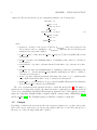
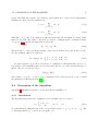
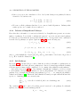
1
User’s Manual
Software Version: 1.5
Date: Dec 18, 2015
Pumpkin Tool
Aram H. Markosyan
c 2013-2015 Aram H Markosyan. All rights reserved.
Copyright PumpKin: A tool to find principal pathways in plasma chemical models
c 2013 - 2015 Aram H Markosyan.
Copyright This program is free software; you can redistribute it and/or modify it under the terms of the
GNU General Public License as published by the Free Software Foundation; either version 2 of the
License, or (at your option) any later version.
This program is distributed in the hope that it will be useful, but WITHOUT ANY WARRANTY;
without even the implied warranty of MERCHANTABILITY or FITNESS FOR A PARTICULAR
PURPOSE. See the GNU General Public License for more details.
You should have received a copy of the GNU General Public License along with this program;
if not, write to the Free Software Foundation, Inc., 51 Franklin Street, Fifth Floor, Boston, MA
02110-1301, USA.
Permission to use PumpKin under the license GNU GPL (version 2) is hereby granted, provided
that proper reference is made in publications reporting results obtained using this software. At
present, the preferred way to reference PumpKin is as follows:
A.H. Markosyan, A. Luque, F. J. Gordillo-Vzquez, U. Ebert, PumpKin: A tool to find principal
pathways in plasma chemical models; Computer Physics Communications 185, pp. 2697-2702,
(2014), doi:10.1016/j.cpc.2014.05.019
Point of Contact: Dr. Aram H. Markosyan
Address: University of Michigan, Electrical Engineering and Computer Science Department, 1301
Beal Ave, Ann Arbor, MI 48109-2122
Email: [email protected]
Tel: 734-647-4840
Homepage: http://markosyanaram.com
Contents
1 Introduction
1.1 System Requirements
. . . . . . . . . . . . . . . . . . . . . . . . . . . . . . . . . . .
2 Installation and Execution Instructions
2.1 Installation . . . . . . . . . . . . . . . .
2.1.1 Unpackaing the Distribution File
2.1.2 Compiling the Package . . . . . .
2.1.3 Execution Instructions . . . . . .
2.1.4 Running Built-in Examples . . .
2.1.5 Typical Running Time . . . . . .
1
1
.
.
.
.
.
.
3
3
3
4
4
4
4
3 Input and Output
3.1 Input . . . . . . . . . . . . . . . . . . . . . . . . . . . . . . . . . . . . . . . . . . . . .
3.2 Output . . . . . . . . . . . . . . . . . . . . . . . . . . . . . . . . . . . . . . . . . . .
5
5
6
4 Examples
4.1 ZDPlasKin Examples . . . . . . . . . . . . . . . . . . . . . . . . . . . . . . . . . . . .
4.2 Global Kin Examples . . . . . . . . . . . . . . . . . . . . . . . . . . . . . . . . . . . .
9
9
9
.
.
.
.
.
.
.
.
.
.
.
.
.
.
.
.
.
.
.
.
.
.
.
.
.
.
.
.
.
.
.
.
.
.
.
.
.
.
.
.
.
.
.
.
.
.
.
.
.
.
.
.
.
.
.
.
.
.
.
.
.
.
.
.
.
.
.
.
.
.
.
.
.
.
.
.
.
.
.
.
.
.
.
.
.
.
.
.
.
.
.
.
.
.
.
.
.
.
.
.
.
.
.
.
.
.
.
.
.
.
.
.
.
.
.
.
.
.
.
.
.
.
.
.
.
.
.
.
.
.
.
.
.
.
.
.
.
.
.
.
.
.
.
.
Acknowledgements
11
A PumpKin Algorithm
A.1 Basic Definitions . . . . . . . . . . . . . .
A.2 Description of the Algorithm . . . . . . .
A.2.1 Initialization. . . . . . . . . . . . .
A.2.2 Branching-Points. . . . . . . . . .
A.2.3 Merging Pathways. . . . . . . . . .
A.2.4 Deletion of Insignificant Pathways.
A.2.5 Sub-Pathways. . . . . . . . . . . .
GNU General Public License
.
.
.
.
.
.
.
.
.
.
.
.
.
.
.
.
.
.
.
.
.
.
.
.
.
.
.
.
.
.
.
.
.
.
.
.
.
.
.
.
.
.
.
.
.
.
.
.
.
.
.
.
.
.
.
.
.
.
.
.
.
.
.
.
.
.
.
.
.
.
.
.
.
.
.
.
.
.
.
.
.
.
.
.
.
.
.
.
.
.
.
.
.
.
.
.
.
.
.
.
.
.
.
.
.
.
.
.
.
.
.
.
.
.
.
.
.
.
.
.
.
.
.
.
.
.
.
.
.
.
.
.
.
.
.
.
.
.
.
.
.
.
.
.
.
.
.
.
.
.
.
.
.
.
.
.
.
.
.
.
.
.
.
.
.
.
.
.
15
15
17
17
18
18
19
19
21
i
ii
CONTENTS
Chapter 1
Introduction
PumpKin is a user-friendly software package to find all principal pathways, i.e. the dominant
reaction sequences, in chemical reaction systems. The goal is to analyze the production and/or
destruction mechanisms of a certain species of interest, as well as to reduce a complex plasma
chemistry models.
PumpKin was developed by Aram H. Markosyan at CWI (Centrum Wiskunde & Informatica),
Amsterdam under the STW project 10751 “Transient plasmas for air purification” and at IAACSIC (Instituto de Astrofsica de Andaluca - CSIC), Granada during short visits of A.H. Markosyan
to Dr. F.J. Gordillo-Vázquez and Dr. A. Luque under the ESF (European Science Foundation)
grants 5697, 5698, 5297 within the TEA-IS (Thunderstorm effects on the atmosphere-ionosphere
system) activities. A. Luque contributed to the checking and validation of the code.
PumpKin is free software; you can redistribute it and/or modify it under the terms of the GNU
General Public License (as published by the Free Software Foundation) version 2. PumpKin can
be downloaded from the following address: www.pumpkin-tool.org.
You should have received a copy of the GNU General Public License along with this program; if
not, contact Aram H. Markosyan at [email protected] or write to the Free Software Foundation,
Inc., 59 Temple Place, Suite 330, Boston, MA 02111-1307 USA.
1.1
System Requirements
PumpKin is written in the C++ programming language. It has been tested on Mac OS X, Linux OS
and Microsoft Windows. A C++ compiler is required. We have tested PumpKin with the following
compilers: GCC and LLVM. We recommend Windows users to use Cygwin (www.cygwin.com),
which implements a GNU toolchain in the Windows architecture. In general here are the general
requirements:
• To build PumpKin, the GNU version of make (GNUmake) must be installed. The PumpKin
makefile requires GNU make version 3.77 or later. GNU software can be downloaded from
many places, including www.gnu.org/software/make/.
1
2
CHAPTER 1. INTRODUCTION
• A C++ compiler is required. PumpKin makes heavy use of the ISO/IEC 14882 C++ Standard. Some compilers are not fully compliant with this specification, although most are.
PumpKin has been compiled and tested with
– GNU g++ 3.32 or higher.
– LLVM 3.2 or higher
• GLPK (GNU linear programming kit) must be installed [7]. This allows PumpKin to solve
large-scale linear programming (LP) problems. GLPK can be downloaded from www.gnu.
org/software/glpk/. We have tested PumpKin with GLPK version higher than 4.32.
The recommended system requirements depend on the choice of the input parameters and the
problem size. As a reference, in a MacBook Pro 15-inch (Mid 2010) with a CPU Intel Core i5 at
2.4 GHz, 4 GB (1067 MHz DDR3) of RAM memory and the operating system Mac OS X 10.9,
PumpKin runs the examples from the section 4 in about 30 seconds. When the input files are large,
PumpKin will require more time to load them into the computer memory.
Chapter 2
Installation and Execution
Instructions
2.1
Installation
Before installing PumpKin, the user should have installed the GLPK package. For this we recommend tools like MacPorts (www.macports.org) or Fink (www.finkproject.org) for Mac OS X and
package management systems for GNU/Linux distributions. The windows user can get installation
instructions at (http://winglpk.sourceforge.net).
2.1.1
Unpackaing the Distribution File
The PumpKin package is distributed in the form of a packed archive (a tarball ). It is one file named
pumpkin-X.Y.tar.gz, where X is the major version number and Y is the minor version number; for
example, the archive name might be pumpkin-1.1.tar.gz. In order to prepare the distribution
for installation you should:
1. Copy the PumpKin distribution file to a working directory.
2. Unpack the distribution file with the following command:
$ gzip -d pumpkin-X.Y.tar.gz
After unpacking, the distribution file is automatically renamed to pumpkin-X.Y.tar.
3. Unarchive the distribution file with the following command:
$ tar -x < pumpkin-X.Y.tar
It automatically creates the subdirectory pumpkin-X.Y containing the PumpKin distribution.
4. Alternatively, the user can combine items 2. and 3. using
$ tar -xzf pumpkin-X.Y.tar.gz
3
4
CHAPTER 2. INSTALLATION AND EXECUTION INSTRUCTIONS
2.1.2
Compiling the Package
After unpacking and unarchiving the PumpKin distribution you can compile (build) the package.
For this, normally, you should just type
$ cd pumpkin-X.Y/src
$ make
Advanced users may want to modify the Makefile to change compiler or the location of GLPK.
2.1.3
Execution Instructions
The user can run PumpKin by typing the following command:
$ ./pumpkin [input folder]
where [input folder] is the location of the input folder. If the user doesn’t specify the location of
input folder, PumpKin by default will look it in the current folder, i.e. pumpkin-X.Y/src/Input.
2.1.4
Running Built-in Examples
The most current version of PumpKin (versions 1.1 and higher) is coming with a native support of
ZDPlasKin and Global Kin modeling platforms.
PumpKin is distributed with the following example folders which are discussed in section 4.
Examples are located in the following folders:
pumpkin-X.Y/src/Examples/ZDPlasKin/Input_10
pumpkin-X.Y/src/Examples/ZDPlasKin/Input_20
The user can run PumpKin with the examples by:
./pumpkin Examples/ZDPlasKin/Input_10
./pumpkin Examples/ZDPlasKin/Input_20
or by
./pumpkin Examples/Global_Kin
2.1.5
Typical Running Time
The typical running time of the examples from the section 2.1.4 is around 30 seconds on the
MacBook Pro 15-inch (Mid 2010) with a CPU Intel Core i5 at 2.4 GHz, 4 GB (1067 MHz DDR3)
of RAM memory and the operating system Mac OS X 10.9.
Generally speaking PumpKin runtime depends on problem size as loading large input files into
the computer memory might be time consuming. On the other hand the user’s choice of the input
parameters discussed in the section 3.1 will also affect the runtime. For typical use cases we estimate
runtime in the order of minutes.
Chapter 3
Input and Output
3.1
Input
To determine the chemical pathways, PumpKin requires from the user the stoichiometric matrix
and kinetic data for the full chemical reaction system, namely:
• chemical reactions Rj , j = 1, . . . , nR , involving between species Si , i = 1, . . . , nS , where nR
and nS are the number of chemical reactions and species, respectively,
• stoichiometric coefficients sij , which represent the number of molecules of species Si produced
(or negative number of molecules of Si consumed) by reaction Rj ,
• a time evolution of concentrations ci (tl ) and reactions rate rj (tl ), where l = 1, . . . , nT and
t0 = t1 ≤ . . . ≤ tnT = tend ,
The code is independent of the units chosen by the user. Conventionally, ci (tl ) is specified in units
of [mol cm−3 ] and rj in units of [mol cm−3 s−1 ].
PumpKin expects that user stores data in the following files:
qt_species_list.txt: Contains the names of species included in the model.
qt_reactions_list.txt Contains human-readable reaction signatures.
qt_conditions.txt Contains the time steps tl (see A.1) resulting from the simulation.
qt_matrix.txt Contains the stoichiometric matrix of the chemical model.
qt_densities.txt Contains the time-dependent densities of each species at times tl .
qt_rates.txt Contains the time-dependent rates of each reaction at times tl .
5
6
CHAPTER 3. INPUT AND OUTPUT
input.txt The user should also provide an input file similar to the following table
interest = 1
t init = 0.0
t end = 1.0e-3
max bp = 0
tau lifetime = 0.9e-5
(*)
max path = 1500
f min = 0
global kin = 1,
where:
• interest - an index of the species of interest Sinterest , if the user is interested in
the production and/or consumption of Sinterest . Otherwise the user should specify
interest as a non-positive number,
• [t init, t init] - a time interval [t init, t init]⊆ [0, T ] where PumpKin will perform
the analysis,
• max bp - if positive, the maximum number of branching points considered, otherwise it
is disregarded,
• tau lifetime - if positive, a lifetime threshold with units of [s], otherwise it is disregarded,
• max path - if positive, the maximum number of pathways considered per branching point
treatment, i.e. only the first max path pathways with higher rate will be considered,
otherwise it is disregarded,
• f min - if positive, pathway rate threshold in units of [mol cm−3 s−1 ], i.e. pathways with
a rate smaller than f min will be deleted, otherwise it is disregarded.
• global kin - boolean parameter. If 1 (or true) PumpKin will interpret the input files
as from Global Kin, otherwise from ZDPlaskin.
The order of parameters in the input file should be exactly like in the table (*). The names of
parameters are not important. On the other hand, the names of input files are very important. In
order to keep compatibility with VMS/VAX systems, the input files can be all in capitals, except the
input.txt. Currently, PumpKin is fully compatible with the output formats of ZDPlasKin [8, 4, 6]
and Global Kin [3, 2]. The PumpKin package is distributed examples of input files.
3.2
Output
Depending on whether the user has specified the interest parameter as a positive integer (the
index of the species of interest) or as a non-positive number (the user does not have any species of
interest), one of the following results will be printed:
3.2. OUTPUT
7
interest > 0: PumpKin will output all the pathways (and their rates) producing or consuming
the species of interest Sinterest , as well as the relative production or consumption compared with
the initial concentration of Sinterest . The output will also contain information such as how much
Sinterest has been produced or consumed by the pathways that are deleted by PumpKin using
parameters f min or max path.
interest ≤ 0: PumpKin will output all the pathways (and their rates) sorted by rate. In some
cases, this number can be very large, so we decided to limit it by 100, which of course can be easily
changed inside the PumpKin source code. The output will also contain information such as the
amount of a certain species that has been produced or consumed by the pathways that are deleted
by PumpKin according to the parameters f min or max path.
After successful first run, PumpKin will ask user to enter a new species of interest. In this
case, PumpKin will not perform any actual pathway analysis (and save a lot of time!), but only
will print for a given input file (with a new species of interest) the production/ consumption of the
new species of interest. User can type 0 to see the dominant pathways or a negative number to
terminate execution.
8
CHAPTER 3. INPUT AND OUTPUT
Chapter 4
Examples
The most current version of PumpKin (versions 1.1 and higher) is coming with a native support of
ZDPlasKin and Global Kin modeling platforms.
4.1
ZDPlasKin Examples
PumpKin is distributed with two sets of input files from ZDPlasKin:
pumpkin-X.Y/src/Examples/ZDPlasKin/Input_10
pumpkin-X.Y/src/Examples/ZDPlasKin/Input_20
Both examples are the outputs of the zero-dimensional plasma kinetic solver ZDPlasKin. We
use a zero-dimensional model to describe the dynamics of species under a constant electric field.
The following system of ordinary differential equations (ODEs) is used to describe the interaction
between the species
d[ni ]
= Si ,
(4.1)
dt
where the source term Si is the total production and destruction rate of species i in various processes.
The adapted version of the kinetic file for N2 -O2 mixtures (dry air) from ZDPlasKin [8, 4] is used,
which consists of 650 reactions and 53 species from the table 4.1.
A complete list of plasma chemical precesses in N2 -O2 mixtures is taken mainly from [1]. Transport parameters and constant rates for electron-neutral interactions are calculated using the BOLSIG+ solver built-in into the ZDPlasKin. As initial value of the electron density we use ne (0) =
4.0 · 1013 cm−3 .
The list of species and reactions was automatically converted into a system of ordinary differential equations (4.1) and solved numerically using the ZDPlasKin tool. The user can visualize the
results of ZDPlasKin using the open-source software QtPlaskin [6].
4.2
Global Kin Examples
Available soon.
9
10
CHAPTER 4. EXAMPLES
Table 4.1: Species considered in the model
Ground neutrals
N, N2 , O, O2 , O3
NO, NO2 , NO3
N2 O, N2 O5
Positive ions
+
+
N+ , N +
2 , N3 , N4
+
O+ , O+
2 , O4
+
+
+
NO , N2 O , NO+
2 , O 2 N2
Excited neutrals
3
3
01 −
N2 (A3 Σ+
u , B Πg , C Πu , a Σu )
2
2
1
1
N( D, P), O( D, S)
O2 (a1 ∆g , b1 Σ+
g , 4.5 eV)
O2 (X3 , v = 1 - 4), N2 (X1 , v = 1 - 8)
Negative ions
−
−
e, O− , O−
2 , O3 , O4
−
−
NO− , NO−
2 , NO3 , N2 O
Acknowledgements
The authors acknowledge the support from STW-project 10751, part of the Netherlands’s Organization for Scientific Research (NWO). The authors also acknowledge the support from the
European Science Foundation (ESF) for short visit grants 5297, 5697 and 5698 within the ESF
Research Network Program (RNP) entitled Thunderstorm effects on the atmosphere-ionosphere
system (TEA-IS).
11
12
CHAPTER 4. EXAMPLES
Bibliography
[1] M Capitelli, Ferreira C. M., Gordiets B. F., and Osipov A. I. Plasma Kinetics in Atmospheric
Gases. Springer Verlag, Berlin, Germany, 2000. 9
[2] R. Dorai and M. J. Kushner. A model for plasma modification of polypropylene using atmospheric pressure discharges. J. Phys. D, 36:666, 2003. 6
[3] Rajesh Dorai and Mark J Kushner. Repetitively pulsed plasma remediation of no x in soot
laden exhaust using dielectric barrier discharges. Journal of Physics D: Applied Physics,
35(22):2954, 2002. 6
[4] A. Flitti and S. Pancheshnyi. Gas heating in fast pulsed discharges in N2 -O2 mixtures. European
Physical Journal Applied Physics, 45(2):021001, 2009. 6, 9
[5] R. Lehmann. An algorithm for the determination of all significant pathways in chemical
reaction systems. Journal of Atmospheric Chemistry, 47(1):45–78, 2004. 15, 18, 19, 20
[6] A. Luque. Computer code QPlaskin. http://www.trappa.es/content/software. 6, 9
[7] A. Makhorin. GNU Linear Programming Kit, 4.9. http://www.gnu.org/software/glpk/. 2,
20
[8] S Pancheshnyi, B. Eismann, G.J.M. Hagelaar, and L.C. Pitchford. Computer code ZDPlasKin
(University of Toulouse, LAPLACE, CNRS-UPS-INP, Toulouse, France, 2008). http://www.
zdplaskin.laplace.univ-tlse.fr. 6, 9
[9] R. Schuster and S. Schuster. Refined algorithm and computer program for calculating all nonnegative fluxes admissible in steady states of biochemical reaction systems with or without
some flux rates fixed. Computer applications in the biosciences: CABIOS, 9(1):79–85, 1993.
19
[10] S. Schuster, C. Hilgetag, J.H. Woods, and D.A. Fell. Reaction routes in biochemical reaction
systems: Algebraic properties, validated calculation procedure and example from nucleotide
metabolism. Journal of Mathematical Biology, 45(2):153–181, 2002. 17, 20
13
14
BIBLIOGRAPHY
Appendix A
PumpKin Algorithm
In this section we briefly describe the algorithm proposed by Lehmann [5] and used in the package
PumpKin. For a more detailed description and discussion about the algorithm we refer to [5].
A.1
Basic Definitions
We assume the chemical reactions Rj , j = 1, . . . , nR , involving species Si , i = 1, . . . , nS . Beside of
Rj , it is assumed that the stoichiometric coefficients sij , which represent the number of molecules
of species Si produced (or negative number of molecules of Si consumed) by reaction Rj , are given.
For simplicity, PumpKin assumes only unidirectional reactions and in case of reversible reactions,
it is the responsibility of the user to split them into forward and backward steps, incorporating
external sources and sinks as “pseudo-reactions”.
We assume that the user has already integrated the chemical model, following the temporal
evolution of species Si during the time interval [0, T ] which was divided, in general non-uniformly,
into nT parts. That is, for every species Si and reaction Rj we know the concentrations ci (tl ) and
the reaction rates rj (tl ), where l = 1, . . . , nT .
For a given time interval [t0 , tend ] ⊆ [0, T ] we can calculate
∆ci = ci (tend ) − ci (t0 ),
1
·
∆t
Z
1
·
rj =
∆t
Z
ci =
i = 1, . . . , nS ,
(A.1)
ci (t) dt,
i = 1, . . . , nS ,
(A.2)
rj (t) dt,
j = 1, . . . , nR ,
(A.3)
tend
t0
tend
t0
where ∆t = tend − t0 , ∆ci and ci are, respectively, the change of the concentration and the mean
concentration of species Si in the time window [t0 , tend ]; rj is the mean rate of the reaction Rj in the
time interval [t0 , tend ]. In the rest of this paper we will use rate for rj , omitting the attribute mean.
In this work we assume that ci has units of [molecules cm−3 ] and that rj has units of [molecules
cm−3 s−1 ].
15
16
APPENDIX A. PUMPKIN ALGORITHM
Ideally, we should have conservation of the concentration changes ∆ci
∆ci =
nR
X
sij · rj · ∆t,
for every i = 1, . . . , nS ,
(A.4)
j=1
but, due to numerical inaccuracies in the kinetic solver and to the finite time steps, the conservation
(A.4) will usually be violated within the user’s input. We take as the definition of ∆ci the formula
(A.4), instead of (A.1).
One of the key questions that we want to answer is: How, i.e., by the interaction of which
reactions, are certain species produced or destroyed? Obviously, we can determine the reactions
that produce (or destroy) the species directly. But if such a reaction consumes (or produces)
another specie whose chemical lifetime is shorter than the time scale of interest, then it is necessary
to follow the chemical ’fate’ of that species. This leads to the idea of forming pathways, i.e. reaction
sequences, that produce (or destroy) a chemical species of interest.
Let us denote by Pk , where k = 1, . . . , nP , the set of pathways. The given pathway Pk is
described by the set {xjk , mik , fk }, where
• xjk is the multiplicity of reaction Rj in the pathway Pk (zero if Rj does not occur in Pk ),
j = 1, . . . , nR , k = 1, . . . , nP ,
• mik is the positive (negative) number of molecules of Si produced (consumed) by the pathway
Pk , i = 1, . . . , nS , k = 1, . . . , nP ,
• fk is the rate of pathway Pk , k = 1, . . . , nP .
Then, by the definition of xjk and the stoichiometric coefficients sij , we have
mik =
nR
X
sij · xjk .
(A.5)
j=1
If we multiply both sides of (A.5) by fk , we get
mik · fk =
nR
X
sij · (xjk · fk ) ,
(A.6)
j=1
which illustrates that xjk ·fk is the portion of the rate rj of reaction Rj associated with the pathway
Pk .
We take into account the effects of deleted pathways with small rates (in next section). For
this, we introduce the additional variables r̃j , which represent the part of the rate of reaction Rj
associated with the deleted pathways, and p̃i (and d˜i ) representing the rate of the production (and
destruction) of species Si by deleted pathways. In this case, the rate of each reaction will be totally
distributed to pathways, including the effect of the deleted ones
rj = r̃j +
nP
X
k=1
xjk · fk .
(A.7)
A.2. DESCRIPTION OF THE ALGORITHM
17
On the other hand, the total rate of production pi and destruction di of a species Si by all pathways,
including the effect of deleted pathways, are
X
pi = p̃i +
mik · fk ,
(A.8)
mik · fk .
(A.9)
{k | mik >0}
X
di = d˜i +
{k | mik <0}
Although pi , di , p̃i and d˜i are changed at different steps inside the algorithm, we always ensure
that we don’t violate the balance between the production, consumption and concentration change
of a species (A.4) and the following holds at any point:
∆ci = (pi − di ) · ∆t .
(A.10)
The mean rate δi of the concentration change of species Si is defined as ∆ci /∆t. Besides, we also
need the auxiliary variable Di defined as
Di = max{pi , di } =
pi = di + δi if ∆ci > 0 ,
di = pi + |δi | if ∆ci < 0 .
(A.11)
A reaction sequence Pk0 is called sub-pathway of a pathway Pl if all intermediate species, corresponding to the branching-points, are at steady state and the set of all reactions from Pk0 is a
subset of the set of reactions of Pl , i.e.
R(Pk0 ) ⊂ R(Pl ) ,
(A.12)
where R(Pl ) := {j ∈ {1, . . . , nR }|xjl 6= 0}. A pathway is called elementary if it does not contain
sub-pathways (condition(C30 ) from [10]).
A.2
Description of the Algorithm
Algorithm 1 summarizes in pseudo-code the steps in the PumpKin code.
A.2.1
Initialization.
The algorithm starts with a list of pathways, each containing only one reaction:
xjk =
1 if j = k ,
0
else ,
j, k = 1, . . . , nR .
(A.13)
To each pathway we assign the rate of the corresponding reaction, i.e. fk = rk , k = 1, . . . , nR . The
book-keeping variables r̃j , p̃i and d˜i are set equal to zero.
18
APPENDIX A. PUMPKIN ALGORITHM
Algorithm 1 PumpKin algorithm.
1: begin
2: read input files
3: initialize pathways := individual pathways
4: chose branching-point Sb
5: repeat
6:
merge pathways producing Sb with pathways consuming Sb
7:
delete pathways with a rate less than fmin
8:
determine and split sub-pathways
9: until the new branching-point Sb is found
10: ouput
11: end.
A.2.2
{Section 3.1}
{Section A.2.1}
{Section A.2.2}
{Section A.2.3}
{Section A.2.4}
{Section A.2.5}
{Section A.2.5}
Branching-Points.
Depending on the time scale of interest and the lifetime of species of interest, the user might need to
exclude certain species from the list of branching points. For this, user can define lifetime threshold
τmin . In this case the species with lifetime greater than τmin are considered as long-lived species
and not used as branching points. Then, for every species Si with a lifetime shorter than τmin and
that has not been a branching point yet, we calculate its lifetime τi with respect to the pathways
constructed so far:
ci
τi = ,
(A.14)
di
with ci from (A.2) and di from (A.9). As the next branching point we choose the species with the
shortest lifetime τi .
A.2.3
Merging Pathways.
Let us assume that we are given branching-point species Sb and that so far we have constructed
pathways Pk , k = 1, . . . , nP . Then we perform the following steps:
• Every pathway Pk producing the species Sb is connected with each pathway Pl consuming
Sb . Let us denote the resulting pathway by Pn . The number of molecules min of Si and the
corresponding multiplicities xjn of the reactions Rj in the pathway Pn can be calculated as
min = mik · |mbl | + mil · mbk ,
xjn = xjk · |mbl | + xjl · mbk ,
i = 1, . . . , nS ,
(A.15)
j = 1, . . . , nR .
(A.16)
Equation (A.15) ensures that the constructed pathway Pn fully recycles Sb , that is, it has no
net production or consumption of Sb .
The rate fn of the new pathway Pn is calculated using the branching probabilities discussed
in [5] and reads
fk · fl
.
(A.17)
fn =
Db
A.2. DESCRIPTION OF THE ALGORITHM
19
• If ∆cb 6= 0, we store the contribution of Pk to ∆cb by introducing a new pathway Pn that is
identical to Pk , but has a rate
fk · δb /Db , if ∆cb > 0
fn =
.
(A.18)
fk · |δb |/Db , if ∆cb < 0
• We remove all the pathways that have been connected with all partners. Pathways that
neither produce nor consume Sb are not affected.
A.2.4
Deletion of Insignificant Pathways.
Even when the total number of reactions is relatively low, PumpKin may generate an excessive
number of pathways. To avoid this “combinatorial explosion”, we delete a newly formed pathway
Pn if its rate fn is less than the user-specified threshold fmin . To keep track of the contribution
from the deleted pathways, we update equations (A.7)-(A.9) in the following way
r̃j := r̃j + xjn · fn ,
j = 1, . . . , nR ,
(A.19)
p̃i := p̃i + min · fn ,
if min > 0,
i = 1, . . . , nS ,
(A.20)
d˜i := d˜i + min · fn ,
if min < 0,
i = 1, . . . , nS ,
(A.21)
where xjn is the multiplicity of reaction Rj in Pn , and min is the number of molecules of Si produced
by Pn . More details are discussed in [5].
A.2.5
Sub-Pathways.
In section A.2.4 we discussed the procedure to limit the growth of total number of pathways in our
algorithm. On the other hand, when two pathways are connected, it may happen that the resulting
reaction sequence is unnecessarily complicated, i.e. it contains other pathways as sub-pathways.
As described in section A.2.4, we often eliminate “insignificant” pathways; so it is not enough
to check whether other pathways constructed so far are sub-pathways of Pn . Instead, for a given
pathway Pn we determine all elementary sub-pathways Pk0 , k = 1, . . . , nP 0 , using the algorithm by
Schuster and Schuster [9, 5]. This method has a limitation, namely, it requires that all intermediate
species, i.e. branching-points, are at steady state
nR
X
xjn · sij = 0 for all i for which Si has been a branching point .
(A.22)
j=1
The condition (A.22) can be enforced by adding “pseudo-reactions” to the pathway Pn , with multiplicity |min | for all previous branching-points Si ,
Si → . . .
if min > 0 ,
(A.23)
20
APPENDIX A. PUMPKIN ALGORITHM
Si ← . . .
if min < 0 .
(A.24)
Once we have the sub-pathways Pk0 , k = 1, . . . , nP 0 , of a pathway Pn , then we represent Pn as a
linear combination (with non-negative wights wk ) of these sub pathways, i.e.
0
xjn =
nP
X
wk · x0jk ,
j = 1, . . . , nR ,
(A.25)
k=1
where xjn and x0jk are the multiplicities of reaction Rj in pathway Pn and subpathway Pk0 , respectively. Such representation is justified in [10]. The rate fn of Pn will be distributed to the
sub-pathways according to
fk0 = wk · fn , k = 1, . . . , nP 0 .
(A.26)
The equation (A.25) leads to a linear optimization problem [5], which we solve by the simplex
method employing the GPLK package [7]. Then, we search for the sub-pathways Pk0 , k = 1, . . . , nP 0 ,
in the list of pathways constructed so far by the main part of the algorithm. If Pk0 is contained in
that list, then we add fk0 to its rate, otherwise, we add Pk0 as a new entry with rate fk0 .
GNU General Public License
Version 2, June 1991
c 1989, 1991 Free Software Foundation, Inc. http://fsf.org/
Copyright Everyone is permitted to copy and distribute verbatim copies of this license document, but changing it
is not allowed.
Preamble
The licenses for most software are designed to take away your freedom to share and change it. By contrast, the
GNU General Public License is intended to guarantee your freedom to share and change free software–to make sure
the software is free for all its users. This General Public License applies to most of the Free Software Foundation’s
software and to any other program whose authors commit to using it. (Some other Free Software Foundation software
is covered by the GNU Lesser General Public License instead.) You can apply it to your programs, too.
When we speak of free software, we are referring to freedom, not price. Our General Public Licenses are designed
to make sure that you have the freedom to distribute copies of free software (and charge for this service if you wish),
that you receive source code or can get it if you want it, that you can change the software or use pieces of it in new
free programs; and that you know you can do these things.
To protect your rights, we need to make restrictions that forbid anyone to deny you these rights or to ask you
to surrender the rights. These restrictions translate to certain responsibilities for you if you distribute copies of the
software, or if you modify it.
For example, if you distribute copies of such a program, whether gratis or for a fee, you must give the recipients
all the rights that you have. You must make sure that they, too, receive or can get the source code. And you must
show them these terms so they know their rights.
We protect your rights with two steps: (1) copyright the software, and (2) offer you this license which gives you
legal permission to copy, distribute and/or modify the software.
Also, for each author’s protection and ours, we want to make certain that everyone understands that there is
no warranty for this free software. If the software is modified by someone else and passed on, we want its recipients
to know that what they have is not the original, so that any problems introduced by others will not reflect on the
original authors’ reputations.
Finally, any free program is threatened constantly by software patents. We wish to avoid the danger that
redistributors of a free program will individually obtain patent licenses, in effect making the program proprietary. To
prevent this, we have made it clear that any patent must be licensed for everyone’s free use or not licensed at all.
The precise terms and conditions for copying, distribution and modification follow.
21
22
APPENDIX A. PUMPKIN ALGORITHM
TERMS AND CONDITIONS FOR COPYING, DISTRIBUTION
AND MODIFICATION
0. This License applies to any program or other work which contains a notice placed by the copyright holder
saying it may be distributed under the terms of this General Public License. The “Program”, below, refers to
any such program or work, and a “work based on the Program” means either the Program or any derivative
work under copyright law: that is to say, a work containing the Program or a portion of it, either verbatim
or with modifications and/or translated into another language. (Hereinafter, translation is included without
limitation in the term “modification”.) Each licensee is addressed as “you”.
Activities other than copying, distribution and modification are not covered by this License; they are outside
its scope. The act of running the Program is not restricted, and the output from the Program is covered only
if its contents constitute a work based on the Program (independent of having been made by running the
Program). Whether that is true depends on what the Program does.
1. You may copy and distribute verbatim copies of the Program’s source code as you receive it, in any medium,
provided that you conspicuously and appropriately publish on each copy an appropriate copyright notice and
disclaimer of warranty; keep intact all the notices that refer to this License and to the absence of any warranty;
and give any other recipients of the Program a copy of this License along with the Program.
You may charge a fee for the physical act of transferring a copy, and you may at your option offer warranty
protection in exchange for a fee.
2. You may modify your copy or copies of the Program or any portion of it, thus forming a work based on the
Program, and copy and distribute such modifications or work under the terms of Section 1 above, provided
that you also meet all of these conditions:
(a) You must cause the modified files to carry prominent notices stating that you changed the files and the
date of any change.
(b) You must cause any work that you distribute or publish, that in whole or in part contains or is derived
from the Program or any part thereof, to be licensed as a whole at no charge to all third parties under
the terms of this License.
(c) If the modified program normally reads commands interactively when run, you must cause it, when
started running for such interactive use in the most ordinary way, to print or display an announcement
including an appropriate copyright notice and a notice that there is no warranty (or else, saying that
you provide a warranty) and that users may redistribute the program under these conditions, and telling
the user how to view a copy of this License. (Exception: if the Program itself is interactive but does
not normally print such an announcement, your work based on the Program is not required to print an
announcement.)
These requirements apply to the modified work as a whole. If identifiable sections of that work are not derived
from the Program, and can be reasonably considered independent and separate works in themselves, then this
License, and its terms, do not apply to those sections when you distribute them as separate works. But when
you distribute the same sections as part of a whole which is a work based on the Program, the distribution
of the whole must be on the terms of this License, whose permissions for other licensees extend to the entire
whole, and thus to each and every part regardless of who wrote it.
Thus, it is not the intent of this section to claim rights or contest your rights to work written entirely by you;
rather, the intent is to exercise the right to control the distribution of derivative or collective works based on
the Program.
In addition, mere aggregation of another work not based on the Program with the Program (or with a work
based on the Program) on a volume of a storage or distribution medium does not bring the other work under
the scope of this License.
3. You may copy and distribute the Program (or a work based on it, under Section 2) in object code or executable
form under the terms of Sections 1 and 2 above provided that you also do one of the following:
A.2. DESCRIPTION OF THE ALGORITHM
23
(a) Accompany it with the complete corresponding machine-readable source code, which must be distributed
under the terms of Sections 1 and 2 above on a medium customarily used for software interchange; or,
(b) Accompany it with a written offer, valid for at least three years, to give any third party, for a charge no
more than your cost of physically performing source distribution, a complete machine-readable copy of
the corresponding source code, to be distributed under the terms of Sections 1 and 2 above on a medium
customarily used for software interchange; or,
(c) Accompany it with the information you received as to the offer to distribute corresponding source code.
(This alternative is allowed only for noncommercial distribution and only if you received the program in
object code or executable form with such an offer, in accord with Subsection b above.)
The source code for a work means the preferred form of the work for making modifications to it. For an executable work, complete source code means all the source code for all modules it contains, plus any associated
interface definition files, plus the scripts used to control compilation and installation of the executable. However, as a special exception, the source code distributed need not include anything that is normally distributed
(in either source or binary form) with the major components (compiler, kernel, and so on) of the operating
system on which the executable runs, unless that component itself accompanies the executable.
If distribution of executable or object code is made by offering access to copy from a designated place, then
offering equivalent access to copy the source code from the same place counts as distribution of the source
code, even though third parties are not compelled to copy the source along with the object code.
4. You may not copy, modify, sublicense, or distribute the Program except as expressly provided under this
License. Any attempt otherwise to copy, modify, sublicense or distribute the Program is void, and will
automatically terminate your rights under this License. However, parties who have received copies, or rights,
from you under this License will not have their licenses terminated so long as such parties remain in full
compliance.
5. You are not required to accept this License, since you have not signed it. However, nothing else grants you
permission to modify or distribute the Program or its derivative works. These actions are prohibited by law
if you do not accept this License. Therefore, by modifying or distributing the Program (or any work based
on the Program), you indicate your acceptance of this License to do so, and all its terms and conditions for
copying, distributing or modifying the Program or works based on it.
6. Each time you redistribute the Program (or any work based on the Program), the recipient automatically
receives a license from the original licensor to copy, distribute or modify the Program subject to these terms
and conditions. You may not impose any further restrictions on the recipients’ exercise of the rights granted
herein. You are not responsible for enforcing compliance by third parties to this License.
7. If, as a consequence of a court judgment or allegation of patent infringement or for any other reason (not
limited to patent issues), conditions are imposed on you (whether by court order, agreement or otherwise)
that contradict the conditions of this License, they do not excuse you from the conditions of this License.
If you cannot distribute so as to satisfy simultaneously your obligations under this License and any other
pertinent obligations, then as a consequence you may not distribute the Program at all. For example, if a
patent license would not permit royalty-free redistribution of the Program by all those who receive copies
directly or indirectly through you, then the only way you could satisfy both it and this License would be to
refrain entirely from distribution of the Program.
If any portion of this section is held invalid or unenforceable under any particular circumstance, the balance
of the section is intended to apply and the section as a whole is intended to apply in other circumstances.
It is not the purpose of this section to induce you to infringe any patents or other property right claims or
to contest validity of any such claims; this section has the sole purpose of protecting the integrity of the
free software distribution system, which is implemented by public license practices. Many people have made
generous contributions to the wide range of software distributed through that system in reliance on consistent
application of that system; it is up to the author/donor to decide if he or she is willing to distribute software
through any other system and a licensee cannot impose that choice.
This section is intended to make thoroughly clear what is believed to be a consequence of the rest of this
License.
24
APPENDIX A. PUMPKIN ALGORITHM
8. If the distribution and/or use of the Program is restricted in certain countries either by patents or by copyrighted interfaces, the original copyright holder who places the Program under this License may add an
explicit geographical distribution limitation excluding those countries, so that distribution is permitted only
in or among countries not thus excluded. In such case, this License incorporates the limitation as if written in
the body of this License.
9. The Free Software Foundation may publish revised and/or new versions of the General Public License from
time to time. Such new versions will be similar in spirit to the present version, but may differ in detail to
address new problems or concerns.
Each version is given a distinguishing version number. If the Program specifies a version number of this License
which applies to it and ”any later version”, you have the option of following the terms and conditions either
of that version or of any later version published by the Free Software Foundation. If the Program does not
specify a version number of this License, you may choose any version ever published by the Free Software
Foundation.
10. If you wish to incorporate parts of the Program into other free programs whose distribution conditions are
different, write to the author to ask for permission. For software which is copyrighted by the Free Software
Foundation, write to the Free Software Foundation; we sometimes make exceptions for this. Our decision will
be guided by the two goals of preserving the free status of all derivatives of our free software and of promoting
the sharing and reuse of software generally.
NO WARRANTY
11. BECAUSE THE PROGRAM IS LICENSED FREE OF CHARGE, THERE IS NO WARRANTY FOR THE
PROGRAM, TO THE EXTENT PERMITTED BY APPLICABLE LAW. EXCEPT WHEN OTHERWISE
STATED IN WRITING THE COPYRIGHT HOLDERS AND/OR OTHER PARTIES PROVIDE THE PROGRAM ”AS IS” WITHOUT WARRANTY OF ANY KIND, EITHER EXPRESSED OR IMPLIED, INCLUDING, BUT NOT LIMITED TO, THE IMPLIED WARRANTIES OF MERCHANTABILITY AND FITNESS
FOR A PARTICULAR PURPOSE. THE ENTIRE RISK AS TO THE QUALITY AND PERFORMANCE
OF THE PROGRAM IS WITH YOU. SHOULD THE PROGRAM PROVE DEFECTIVE, YOU ASSUME
THE COST OF ALL NECESSARY SERVICING, REPAIR OR CORRECTION.
12. IN NO EVENT UNLESS REQUIRED BY APPLICABLE LAW OR AGREED TO IN WRITING WILL
ANY COPYRIGHT HOLDER, OR ANY OTHER PARTY WHO MAY MODIFY AND/OR REDISTRIBUTE
THE PROGRAM AS PERMITTED ABOVE, BE LIABLE TO YOU FOR DAMAGES, INCLUDING ANY
GENERAL, SPECIAL, INCIDENTAL OR CONSEQUENTIAL DAMAGES ARISING OUT OF THE USE
OR INABILITY TO USE THE PROGRAM (INCLUDING BUT NOT LIMITED TO LOSS OF DATA OR
DATA BEING RENDERED INACCURATE OR LOSSES SUSTAINED BY YOU OR THIRD PARTIES OR
A FAILURE OF THE PROGRAM TO OPERATE WITH ANY OTHER PROGRAMS), EVEN IF SUCH
HOLDER OR OTHER PARTY HAS BEEN ADVISED OF THE POSSIBILITY OF SUCH DAMAGES.
END OF TERMS AND CONDITIONS