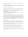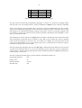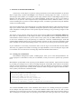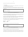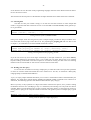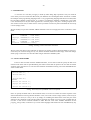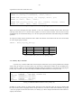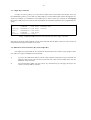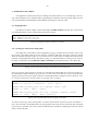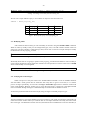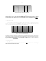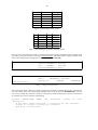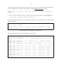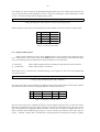
Download A Primer on SQL (1st Edition)

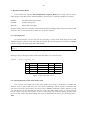
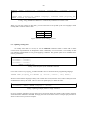
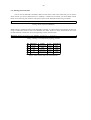
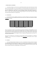
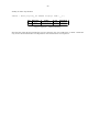
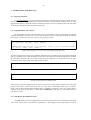
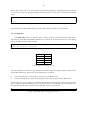
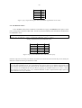
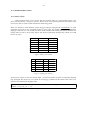
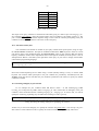
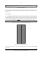
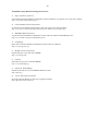
A Primer on SQL (1st Edition)
Rahul Batra
18 October 2012
TABLE OF CONTENTS
i)
Licensing
ii)
Preface
iii)
Acknowledgements
1)
An Introduction to SQL
2)
Getting your Database ready
3)
Constraints
4)
Operations on Tables
5)
Writing Basic Queries
6)
Manipulating Data
7)
Organizing your Data
8)
Doing more with Queries
9)
Aggregation and Grouping
10)
Understanding Joins
iv)
Appendix: Major Database Management Systems
v)
Glossary
-2-
To Mum and Dad
-3-
LICENSING
Copyright (c) 2012 by Rahul Batra. This material may be distributed only subject to the terms and conditions set forth in the Open Publication License, v1.0 or later (the latest version is presently available at
http://www.opencontent.org/openpub/).
Distribution of substantively modified versions of this document is prohibited without the explicit permission of the copyright holder.
Distribution of the work or derivative of the work in any standard (paper) book form is prohibited unless
prior permission is obtained from the copyright holder.
All trademarks and trade names are the properties of their respective owners.
Open Publication License
v1.0, 8 June 1999
I. REQUIREMENTS ON BOTH UNMODIFIED AND MODIFIED VERSIONS
The Open Publication works may be reproduced and distributed in whole or in part, in any medium physical or electronic, provided that the terms of this license are adhered to, and that this license or an incorporation of it by reference (with any options elected by the author(s) and/or publisher) is displayed in the reproduction.
Proper form for an incorporation by reference is as follows: Copyright (c) <year> by <author’s name or
designee>. This material may be distributed only subject to the terms and conditions set forth in the Open
Publication License, vX.Y or later (the latest version is presently available at http://www.opencontent.org/openpub/).
The reference must be immediately followed with any options elected by the author(s) and/or publisher of
the document (see section VI).
Commercial redistribution of Open Publication-licensed material is permitted.
Any publication in standard (paper) book form shall require the citation of the original publisher and
author. The publisher and author’s names shall appear on all outer surfaces of the book. On all outer surfaces of the book the original publisher’s name shall be as large as the title of the work and cited as possessive with respect to the title.
II. COPYRIGHT
The copyright to each Open Publication is owned by its author(s) or designee.
III. SCOPE OF LICENSE
The following license terms apply to all Open Publication works, unless otherwise explicitly stated in the
document.
Mere aggregation of Open Publication works or a portion of an Open Publication work with other works or
programs on the same media shall not cause this license to apply to those other works. The aggregate work
shall contain a notice specifying the inclusion of the Open Publication material and appropriate copyright
notice.
-4-
SEVERABILITY. If any part of this license is found to be unenforceable in any jurisdiction, the remaining
portions of the license remain in force.
NO WARRANTY. Open Publication works are licensed and provided "as is" without warranty of any kind,
express or implied, including, but not limited to, the implied warranties of merchantability and fitness for a
particular purpose or a warranty of non-infringement.
IV. REQUIREMENTS ON MODIFIED WORKS
All modified versions of documents covered by this license, including translations, anthologies, compilations and partial documents, must meet the following requirements: The modified version must be labeled
as such.
The person making the modifications must be identified and the modifications dated.
Acknowledgement of the original author and publisher if applicable must be retained according to normal
academic citation practices.
The location of the original unmodified document must be identified.
The original author’s (or authors’) name(s) may not be used to assert or imply endorsement of the resulting
document without the original author’s (or authors’) permission.
V. GOOD-PRACTICE RECOMMENDATIONS
In addition to the requirements of this license, it is requested from and strongly recommended of redistributors that: If you are distributing Open Publication works on hardcopy or CD-ROM, you provide email notification to the authors of your intent to redistribute at least thirty days before your manuscript or media
freeze, to give the authors time to provide updated documents. This notification should describe modifications, if any, made to the document. All substantive modifications (including deletions) be either clearly
marked up in the document or else described in an attachment to the document. Finally, while it is not
mandatory under this license, it is considered good form to offer a free copy of any hardcopy and CD-ROM
expression of an Open Publication-licensed work to its author(s).
VI. LICENSE OPTIONS
The author(s) and/or publisher of an Open Publication-licensed document may elect certain options by
appending language to the reference to or copy of the license. These options are considered part of the
license instance and must be included with the license (or its incorporation by reference) in derived works.
A. To prohibit distribution of substantively modified versions without the explicit permission of the
author(s). "Substantive modification" is defined as a change to the semantic content of the document, and
excludes mere changes in format or typographical corrections.
To accomplish this, add the phrase ’Distribution of substantively modified versions of this document is prohibited without the explicit permission of the copyright holder.’ to the license reference or copy.
B. To prohibit any publication of this work or derivative works in whole or in part in standard (paper) book
form for commercial purposes unless prior permission is obtained from the copyright holder.
To accomplish this, add the phrase ’Distribution of the work or derivative of the work in any standard
(paper) book form is prohibited unless prior permission is obtained from the copyright holder.’ to the
license reference or copy.
-5-
PREFACE
Welcome to the first edition of A Primer on SQL. As you would be able to see, the book is fairly
short and is intended as an introduction to the basics of SQL. No prior experience with SQL is necessary,
but some knowledge of working with computers in general is required. My purpose of writing this was to
provide a gentle tutorial on the syntax of SQL, so that the reader is able to recognize the parts of queries
they encounter and even be able to write simple SQL statements and queries themselves. The book however
is not intended as a reference work or for a full time database administrator since it does not have an exaustive topic coverage.
For the curious, the book was typeset using Troff and its ms macro set. Give it a whirl, its quite powerful.
Your questions, comments, criticism, encouragement and corrections are most welcome and you can e-mail
me at rhlbatra[aht]hotmail[dot]com. I’ll try answering all on-topic mails and will try to include suggestions, errors and omissions in future editions.
Rahul Batra (8th October 2012)
-6-
ACKNOWLEDGEMENTS
This work would not have been completed without the support of my family and friends. A big thank
you is in order for my lovely wife Pria, who not only acted as an editor but also constantly supported and
cheered me on to complete it. Many thanks to my parents too, who got me a computer early in life to start
tinkering around with and for constantly encouraging me to pursue my dreams.
Thanks also go out to my sister and niece (may you have a beautiful life ahead) and my friends for bringing
much happiness into my life. Finally I would like to acknowledge the contribution of my teachers who
helped me form my computing knowledge.
-7-
1. AN INTRODUCTION TO SQL
A database is nothing but a collection of organized data. It doesn’t have to be in a digital format to
be called a database. A telephone directory is a good example, which stores data about people and organizations with a contact number. Software which is used to manage a digital database is called a Database
Management System (DBMS).
The most prevalent database organizational model is the Relational Model, developed by Dr. E F Codd in
his groundbreaking research paper - A Relational Model of Data for Large Shared Data Banks. In this
model, data to be stored is organized as rows inside a table with the column headings specifying the corresponding type of data stored. This is not unlike a spreadsheet where the first row can be thought of as column headings and the subsequent rows storing the actual data.
SQL stands for Structured Query Language and it is the de-facto standard for interacting with relational
databases. Almost all database management systems you’ll come across will have a SQL implementation.
SQL was standardized by the American National Standards Institute (ANSI) in 1986 and has undergone
many revisions. However, all DBMS’s do not strictly adhere to the standard defined but rather remove some
features and add others to provide a unique feature set. Nonetheless, the standardization process has been
helpful in giving a uniform direction to the vendors in terms of their interaction language.
1.1. SQL Commands Classification
SQL is a language for interacting with databases. It consists of a number of commands with further
options to allow you to carry out your operations with a database. While DBMS’s differ in the command
subset they provide, usually you would find the classifications below.
1. Data Definition Language (DDL): CREATE TABLE, ALTER TABLE, DROP TABLE etc.
These commands allow you to create or modify your database structure.
2. Data Manipulation Language (DML): INSERT, UPDATE, DELETE
These commands are used to manipulate data stored inside your database.
3. Data Query Language (DQL): SELECT
Used for querying or selecting a subset of data from a database.
4. Data Control Language (DCL): GRANT, REVOKE etc.
Used for controlling access to data within a database, commonly used for granting user privileges.
Besides these, your database management system may give you other sets of commands to work more efficiently or to provide extra features. But it is safe to say that the ones above would be present in almost all
DBMS’s you encounter.
1.2. Explaining Tables
A table in a relational database is nothing but a matrix of data where the columns describe the type of
data and the row contains the actual data to be stored. Have a look at the figure below to get a sense of the
visualization of a table in a database.
-8-
id
1
2
3
language
Fortran
Lisp
Cobol
author
Backus
McCarthy
Hopper
year
1955
1958
1959
Figure: a table describing Programming Languages
The above table stores data about programming languages. It consists of 4 columns (id, language, author
and year) and 3 rows. The formal term for a column in a database is a field and a row is known as a record.
There are two things of note in the figure above. The first one is that, the id field effectively tells you nothing about the programming language by itself, other than its sequential position in the table. The second is
that though we can understand the fields by looking at their names, we have not formally assigned a data
type to them i.e. we have not restricted (not yet anyways) whether a field should contain alphabets or numbers or a combination of both.
The id field here serves the purpose of a primary key in the table. It makes each record in the table unique
and its advantages will become clearer in chapters to come. But for now consider this, what if a language
creator made two languages in the same year; we would have a difficult time narrowing down on the
records. An id field usually serves as a good primary key since it’s guaranteed to be unique, but usage of
other fields for this purpose is not restricted.
Just like programming languages, SQL also has data types to define the kind of data that will be stored in
its fields. In the table given above, we can see that the fields language and author must store English language characters. Thus their data type during table creation should be specified as varchar which stands for
variable number of characters.
The other commonly used data types you will encounter in subsequent chapters are:
Fixed length characters
char
Integer values
int
Decimal numbers
decimal
Date data type
date
-9-
2. GETTING YOUR DATABASE READY
The best way to learn SQL is to practice writing commands on a real relational database. In this book
SQL is taught using a product called Ingres. The reasons for choosing Ingres are simple - it comes in a
free and open source edition, it’s available on most major platforms and it’s a full-fledged enterprise class
database with many features. However, any relational database product that you can get your hands on
should serve you just fine. There might be minor incompatibilities between different vendors, so if you
choose something else to practice on while reading this book, it would be a good idea to keep the database
vendor’s user manual handy.
Since this text deals largely with teaching SQL in a product independent manner, rather than the teaching of
Ingres per se, details with respect to installation and specific operations of the product will be kept to a minimum. Emphasis is instead placed on a few specific steps that will help you to get working on Ingres as fast
as possible.
The current version of Ingres during the writing of the book was 10.1 and the Community Edition has
been used on a Windows box for the chapters to follow. The installation itself is straightforward like any
other Windows software. However if you are unsure on any option, ask your DBA (database administrator,
in case one is available) or if you are practicing on a home box - select the ’Traditional Ingres’ mode and
install the Demo database when it asks you these questions. Feel free to refer to the Ingres installation guide
that is available on the web at the following location. http://docs.actian.com/ingres/10.0/installation-guide
If your installation is successful, you should be able to start the Ingres Visual DBA from the Start Menu.
This utility is a graphical user interface to manage your Ingres databases, but we will keep the usage of this
to a minimum since our interest lies in learning SQL rather than database administration.
2.1. Creating your own database
Most database management systems, including Ingres, allow you to create multiple databases. For
practice purposes it’s advisable to create your own database, so that you are free to perform any operations
on it.
Most database systems differ in the way they provide database creation facilities. Ingres achieves the same
by providing you multiple ways to do this, including through the Visual DBA utility. However for didactic
purposes, we will instead use a command operation to create our database. Open up the Ingres Command
Prompt from the program menu (usually found inside Start Menu->Programs->Ingres for Microsoft Windows systems), and enter the command as below.
C:\Documents and Settings\rahulb>createdb testdb
Creating database ’testdb’ . . .
Creating DBMS System Catalogs . . .
Modifying DBMS System Catalogs . . .
Creating Standard Catalog Interface . . .
Creating Front-end System Catalogs . . .
Creation of database ’testdb’ completed successfully.
Listing: using createdb and its sample output
The command createdb is used to create a database which will serve as a holding envelope for your tables.
In the example and output shown above, we created a database called testdb for our use. You (or more
specifically your system login) are now the owner of this database and have full control of entities within it.
This is analogous to creating a file in an operating system where the creator gets full access control rights
-10-
and may choose to give other users and groups specific rights.
2.2. Table Creation
We have already explored the concept of a table in a relational model. It is now time to create one
using a standard SQL command - CREATE TABLE.
Note: the SQL standard by definition allows commands and keywords to be written in a case insensitive
manner. In this book we would use uppercase letters while writing them in statements, which is a widely
accepted practice.
CREATE TABLE <Table_Name>
(<Field 1> <Data Type>,
<Field 2> <Data Type>,
. . .
<Field N> <Data Type>);
Listing: General Syntax of a CREATE TABLE statement
This is the simplest valid statement that will create a table for you, devoid of any extra options. We’ll further this with clauses and constraints as we go along, but for now let us use this general syntax to actually
create the table of programming languages we introduced in Chapter 1.
The easiest way to get started with writing SQL statements in Ingres is to use their Visual SQL application
which gives you a graphical interface to write statements and view output. The usual place to find it on a
Windows system is Start -> Programs -> Ingres -> Ingres II -> Other Utilities.
When you open it up, it gives you a set of dropdown boxes on the top half of the window where you can
select the database you wish to work upon and other such options. Since we’ll be using the same database
we created previously (testdb), go ahead and select the options as specified below.
Default User
Default Server
Database
<your username>
INGRES
testdb
The actual SQL statement you would be writing to create your table is given below.
CREATE TABLE proglang_tbl (
id
INTEGER,
language VARCHAR(20),
author
VARCHAR(25),
year
INTEGER);
Listing: Creating the programming languages table
Press the ’Go’ or F5 button when you’re done entering the query in full. If you get no errors back from Visual SQL, then congratulations are in order since you’ve just created your first table.
The statement by itself is simple enough since it resembles the general syntax of CREATE TABLE we discussed beforehand. It is interesting to note the data types chosen for the fields. Both id and year are specified as integers for simplicity, even though there are better alternatives. The language field is given a space
-11-
of 20 characters to store the name of the programming language while the author field can hold 25 characters for the creator’s name.
The semicolon at the last position is the delimiter for SQL statements and it marks the end of a statement.
2.3. Inserting data
The table we have just created is empty so our task now becomes insertion of some sample data
inside it. To populate this data in the form of rows we use the DML command INSERT, whose general syntax is given below.
INSERT INTO <Table Name>
VALUES (’Value1’, ’Value2’, . . .);
Listing: General syntax of INSERT TABLE
Fitting some sample values into this general syntax is simple enough, provided we keep in mind the structure of the table we are trying to insert the row in. For populating the proglang_tbl with rows like we saw
in chapter 1, we would have to use three INSERT statements as below.
INSERT INTO proglang_tbl VALUES (1, ’Fortran’, ’Backus’, 1955);
INSERT INTO proglang_tbl VALUES (2, ’Lisp’, ’McCarthy’, 1958);
INSERT INTO proglang_tbl VALUES (3, ’Cobol’, ’Hopper’, 1959);
Listing: Inserting data into the proglang_tbl table
If you do not receive any errors from Ingres Visual SQL (or the SQL interface for your chosen DBMS),
then you have managed to successfully insert 3 rows of data into your table. Notice how we’ve carefully
kept the ordering of the fields in the same sequence as we used for creating our table. This strict ordering
limitation can be removed and we will see how to achieve that in a little while.
2.4. Writing your first query
Let us now turn our attention to writing a simple query to check the results of our previous operations
in which we created a table and inserted three rows of data into it. For this, we would use a Data Query
Language (DQL) command called SELECT.
A query is simply a SQL statement that allows you to retrieve a useful subset of data contained within your
database. You might have noticed that the INSERT and CREATE TABLE commands were referred to as
statements, but a fetching operation with SELECT falls under the query category.
Most of your day to day operations in a SQL environment would involve queries, since you’d be creating
the database structure once (modifying it only on a need basis) and inserting rows only when new data is
available. While a typical SELECT query is fairly complex with many clauses, we will begin our journey by
writing down a query just to verify the contents of our table. The general syntax of a simple query is given
below.
SELECT <Selection> FROM <Table Name>;
Listing: General Syntax of a simple SQL query
-12-
Transforming this into our result verification query is a simple task. We already know the table we wish to
query - proglang_tbl and for our selection we would use * (star), which will select all rows and fields from
the table.
SELECT * FROM proglang_tbl;
The output of this query would be all the (3) rows displayed in a matrix format just as we intended. If you
are running this through Visual SQL on Ingres, you would get a message at the bottom saying - Total
Fetched Row(s): 3.
-13-
3. CONSTRAINTS
A constraint is a rule that you apply or abide by while doing SQL operations. They are useful in
cases where you wish to make the data inside your database more meaningful and/or structured. Consider
the example of the programming languages table - every programming language that has been created, must
have an author (whether a single person, or a couple or a committee). Similarly it should have a year when
it was introduced, be it the year it first appeared as a research paper or the year a working compiler for it
was written. In such cases, it makes sense to create your table in such a way that certain fields do not accept
a NULL (empty) value.
We now modify our previous CREATE TABLE statement so that we can apply the NULL constraint to some
fields.
CREATE TABLE proglang_tblcopy (
id
INTEGER
NOT NULL,
language VARCHAR(20) NOT NULL,
author
VARCHAR(25) NOT NULL,
year
INTEGER
NOT NULL,
standard VARCHAR(10) NULL);
Listing: Creating a table with NULL constraints
We see in this case that we have achieved our objective of creating a table in which the field’s id, language,
author and year cannot be empty for any row, but the new field standard can take empty values. We now go
about trying to insert new rows into this table using an alternative INSERT syntax.
3.1. Selective fields INSERT
From our last encounter with the INSERT statement, we saw that we had to specify the data to be
inserted in the same order as specified during the creation of the table in question. We now look at another
variation which will allow us to overcome this limitation and handle inserting rows with embedded NULL
values in their fields.
INSERT INTO <Table_Name>
(<Field Name 1>,
<Field Name 2>,
. . .
<Field Name N>)
VALUES
(<Value For Field 1>,
<Value For Field 2>,
. . .
<Value For Field N>);
Listing: General Syntax of INSERT with selected fields
Since we specify the field order in the statement itself, we are free to reorder the values sequence in the
same statement thus removing the first limitation. Also, if we wish to enter a empty (NULL) value in any of
the fields for a record, it is easy to do so by simply not including the field’s name in the first part of the
statement. The statement would run fine without specifying any fields you wish to omit provided they do
not have a NOT NULL constraint attached to them. We now write some INSERT statements for the
proglang_tblcopy table, in which we try to insert some languages which have not been standardized by any
-14-
organizations and some which have been.
INSERT INTO proglang_tblcopy (id, language, author, year, standard)
VALUES (1, ’Prolog’, ’Colmerauer’, ’1972’, ’ISO’);
INSERT INTO proglang_tblcopy (id, language, author, year)
VALUES (2, ’Perl’, ’Wall’, ’1987’);
INSERT INTO proglang_tblcopy (id, year, standard, language, author)
VALUES (3, ’1964’, ’ANSI’, ’APL’, ’Iverson’);
Listing: Inserting new data into the proglang_tblcopy table
When you run this through your SQL interface, 3 new rows would be inserted into the table. Notice the
ordering of the third row; it is not the same sequence we used to create the table. Also Perl has not been
standardized by an international body, so we do not specify the field name itself while doing the INSERT
operation.
To verify the results of these statements and to make sure that the correct data went into the correct fields,
we run a simple query as before.
SELECT * FROM proglang_tblcopy;
id
1
2
3
language
Prolog
Perl
APL
author
Colmerauer
Wall
Iverson
year
1972
1987
1964
standard
ISO
(null)
ANSI
Figure: Result of the query run on proglang_tblcopy
3.2. Primary Key Constraint
A primary key is used to make each record unique in atleast one way by forcing a field to have unique
values. They do not have to be restricted to only one field, a combination of them can also be defined as a
primary key for a table. In our programming languages table, the id field is a good choice for applying the
primary key constraint. We will now modify our CREATE TABLE statement to incorporate this.
CREATE TABLE proglang_tbltmp (
id
INTEGER
NOT NULL PRIMARY KEY,
language VARCHAR(20) NOT NULL,
author
VARCHAR(25) NOT NULL,
year
INTEGER
NOT NULL,
standard VARCHAR(10) NULL);
Listing: a CREATE TABLE statement with a primary key
ID fields are usually chosen as primary fields. Note that in this particular table, the language field would
have also worked, since a language name is unique. However, if we have a table which describes say people
- since two people can have the same name, we usually try to find a unique field like their SSN number or
employee ID number.
-15-
3.3. Unique Key Constraint
A unique key like a primary key is also used to make each record inside a table unique. Once you
have defined the primary key of a table, any other fields you wish to make unique is done through this constraint. For example, in our database it now makes sense to have a unique key constraint on the language
field. This would ensure none of the records would duplicate information about the same programming language.
CREATE TABLE proglang_tbluk (
id
INTEGER
NOT NULL PRIMARY KEY,
language VARCHAR(20) NOT NULL UNIQUE,
author
VARCHAR(25) NOT NULL,
year
INTEGER
NOT NULL,
standard VARCHAR(10) NULL);
Listing: a CREATE TABLE statement with a primary key and a unique constraint
Note that we write the word UNIQUE in front of the field and omit the KEY in this case. You can have as
many fields with unique constraints as you wish.
3.4. Differences between a Primary Key and a Unique Key
You might have noticed that the two constraints discussed above are similar in their purpose. However, there are a couple of differences between them.
1)
A primary key field cannot take on a NULL value, whereas a field with a unique constraint can.
However, there can be only one such record since each value must be unique due to the very
definition of the constraint.
2)
You are allowed to define only one primary key constraint but you can apply the unique constraint to as many fields as you like.
-16-
4. OPERATIONS ON TABLES
You might have noticed that we keep on making new tables whenever we are introducing a new concept. This has had the not-so desirable effect of populating our database with many similar tables. We will
now go about deleting unneeded tables and modifying existing ones to suit our needs.
4.1. Dropping Tables
The deletion of tables in SQL is achieved through the DROP TABLE command. We will now drop
any superfluous tables we have created during the previous lessons.
DROP TABLE proglang_tbl;
DROP TABLE proglang_tblcopy;
DROP TABLE proglang_tbltmp;
Listing: dropping the temporary tables we created
4.2. Creating new tables from existing tables
You might have noticed that we have dropped the proglang_tbl table and we now have with us only
the proglang_tbluk table which has all the necessary constraints and fields. The latter’s name was chosen
when we were discussing the unique key constraint but it now seems logical to migrate this table structure
(and any corresponding data) back to the name proglang_tbl. We achieve this by creating a copy of the table using a combination of both CREATE TABLE and SELECT commands and learn a new clause AS.
CREATE TABLE <New Table> AS SELECT <Selection> FROM <Old Table>;
Listing: general syntax for creating a new table from an existing one
Since our proglang_tbluk contains no records, we will push some sample data in it so that we can later verify whether the records themselves got copied or not. Notice that we would have to give the field names
explicitly, else the second row (which contains no standard field value) would give an error similar to ’number of target columns must equal the number of specified values’ in Ingres.
INSERT INTO proglang_tbluk (id, language, author, year, standard)
VALUES (1, ’Prolog’, ’Colmerauer’, ’1972’, ’ISO’);
INSERT INTO proglang_tbluk (id, language, author, year)
VALUES (2, ’Perl’, ’Wall’, ’1987’);
INSERT INTO proglang_tbluk (id, year, standard, language, author)
VALUES (3, ’1964’, ’ANSI’, ’APL’, ’Iverson’);
Listing: inserting some data into the proglang_tbluk table
To create an exact copy of the existing table, we use the same selection criteria as we have seen before - *
(star). This will select all the fields from the existing table and create the new table with them alongwith
any records. It is possible to use only a subset of fields from the old table by modifying the selection criteria
and we will see this later.
-17-
CREATE TABLE proglang_tbl AS SELECT * FROM proglang_tbluk;
Listing: recreating a new table from an existing one
We now run a simple SELECT query to see whether our objective was achieved or not.
SELECT * FROM proglang_tbl;
id
1
2
3
language
Prolog
Perl
APL
author
Colmerauer
Wall
Iverson
year
1972
1987
1964
standard
ISO
(null)
ANSI
Figure: Result of the query run on proglang_tbl
4.3. Modifying tables
After a table has been created, you can still modify its structure using the ALTER TABLE command.
What we mean by modify is that you can change field types, sizes, even add or delete columns. There are
some rules you have to abide by while altering a table, but for now we will see a simple example to modify
the field author for the proglang_tbl table.
ALTER TABLE <Table name> <Operation> <Field with clauses>;
Listing: General syntax of a simple ALTER TABLE command
We already know that we are going to operate on the proglang_tbl table and the field we wish to modify is
author which should now hold 30 characters instead of 25. The operation to choose in this case is ALTER
which would modify our existing field.
ALTER TABLE proglang_tbl ALTER author varchar(30);
Listing: Altering the author field
4.4. Verifying the result in Ingres
While one option to verify the result of our ALTER TABLE command is to run an INSERT statement
with the author’s name greater than 25 characters and verify that we get no errors back, it is a tedious
process. In Ingres specifically, we can look at the Ingres Visual DBA application to check the columns tab
in the testdb database. However, another way to verify the same using a console tool is the isql command
line tool available through the Ingres Command Prompt we used earlier for database creation.
To launch isql (which stands for Interactive SQL) using the Ingres command prompt we type:
isql testdb
The first argument we write is the database we wish to connect to. The result of running this command is an
interactive console window where you would be able to write SQL statements and verify the results much
like Visual SQL. The difference between the two (other than the obvious differences in the user interface) is
-18-
that isql allows you access to the HELP command, which is what we will be using to verify the result of
our ALTER TABLE statement. In the interaction window that opens up, we write the HELP command as
below and the subsequent box shows the output of the command.
HELP TABLE proglang_tbl;
Name:
Owner:
Created:
Location:
Type:
Version:
Page size:
Cache priority:
Alter table version:
Alter table totwidth:
Row width:
Number of rows:
Storage structure:
Compression:
Duplicate Rows:
Number of pages:
Overflow data pages:
Journaling:
Base table for view:
Permissions:
Integrities:
Optimizer statistics:
proglang_tbl
rahulb
20-feb-2012 17:04:28
ii_database
user table
II10.0
8192
0
4
76
76
3
heap
none
allowed
3
0
enabled after the next checkpoint
no
none
none
none
Column Information:
Column Name
id
language
author
year
standard
Type
integer
varchar
varchar
integer
varchar
Secondary indexes:
Length
4
20
30
4
10
Nulls
no
no
yes
no
yes
Defaults
no
no
null
no
null
Key Seq
none
Figure: the result of running the HELP TABLE command
While there is a lot of information in the result, we are currently interested in the Column Information section which now displays the new length of the author field, i.e. 30. But it is also important to note that our
ALTER TABLE statement just removed the not-null constraint from the field. To retain the same, we would
have to specify the constraint in the ALTER TABLE command since the default behavior is to allow NULL
values.
4.5. Verifying the result in other DBMS’s
The HELP command we just saw is specific to the Ingres RDBMS, it is not a part of the SQL standard. To achieve the same objective on a different RDBMS like Oracle, you are provided with the
DESCRIBE command which allows you to view a table definition. While the information this command
show may vary from one DBMS to another, they at least show the field name, its data type and whether or
-19-
not NULL values are allowed for the particular field. The general synatax of the command is given below.
DESCRIBE <table name>;
Listing: the general syntax of the DESCRIBE statement
-20-
5. WRITING BASIC QUERIES
A query is a SQL statement that is used to extract a subset of data from your database and presents it
in a readable format. As we have seen previously, the SELECT command is used to run queries in SQL.
You can further add clauses to your query to get a filtered, more meaningful result. Since the majority of
operations on a database involve queries, it is important to understand them in detail. While this chapter
will only deal with queries run on a single table, you can run a SELECT operation on multiple tables in a
single statement.
5.1. Selecting a limited number of columns
We have already seen how to extract all the data from a table when we were verifying our results in
the previous chapters. But as you might have noted - a query can be used to extract a subset of data too. We
first test this by limiting the number of fields to show in the query output by not specifying the * selection
criteria, but by naming the fields explicitly.
SELECT language, year FROM proglang_tbl;
Listing: selecting a subset of fields from a table
language
Prolog
Perl
APL
year
1972
1987
1964
Figure: Output of running the chosen fields SELECT query
You can see that the query we constructed mentioned the fields we wish to see, i.e. language and year.
Also note that the result of this query is useful by itself as a report for looking at the chronology of programming language creation. While this is not a rule enforced by SQL or a relation database management
system, it makes sense to construct your query in such a way that the meaning is self-evident if the output is
meant to be read by a human. This is the reason we left out the field id in the query, since it has no inherent
meaning to the reader except if they wish to know the sequential order of the storage of records in the table.
5.2. Ordering the results
You might have noticed that in our previous query output, the languages were printed out in the same
order as we had inserted them. But what if we wanted to sort the results by the year the language was created in. The chronological order might make more sense if we wish to view the development of programming languages through the decades. In such cases, we take the help of the ORDER BY clause. To achieve
our purpose, we modify our query with this additional clause.
SELECT language, year FROM proglang_tbl ORDER BY year;
Listing: Usage of the ORDER BY clause
-21-
language
APL
Prolog
Perl
year
1964
1972
1987
Figure: Output of the ordered SELECT query
The astute reader will notice that the output of our ORDER BY clause was ascending. To reverse this, we
add the argument DESC to our ORDER BY clause as below.
SELECT language, year FROM proglang_tbl ORDER BY year DESC;
Listing: Usage of the ORDER BY clause with the DESC argument
language
Perl
Prolog
APL
year
1987
1972
1964
Figure: Output of the ordered SELECT query in descending order
5.3. Ordering using field abbreviations
A useful shortcut in SQL involves ordering a query result using an integer abbreviation instead of the
complete field name. The abbreviations are formed starting with 1 which is given to the first field specified
in the query, 2 to the second field and so on. Rewriting our above query to sort the output by descending
year, we get:
SELECT language, year FROM proglang_tbl ORDER BY 2 DESC;
language
Perl
Prolog
APL
year
1987
1972
1964
Figure: Output of the ordered SELECT query in descending order using field abbreviations
The 2 argument given to the ORDER BY clause signifies ordering by the second field specified in the query,
namely year.
5.4. Putting conditions with WHERE
We have already seen how to select a subset of data available in a table by limiting the fields queried.
We will now limit the number of records retrieved in a query using conditions. The WHERE clause is used
to achieve this and it can be combined with explicit field selection or ordering clauses to provide meaningful output.
-22-
For a query to run successfully, it must have atleast two parts - the SELECT and the FROM clause. After
this we place the optional WHERE condition and then the ordering clause. Thus, if we wanted to see the
programming language (and it’s author) which was standardized by ANSI, we’d write our query as below.
SELECT language, author FROM proglang_tbl WHERE standard = ’ANSI’;
Listing: Using a WHERE conditional
As you may have noticed, the query we forulated specified the language and author fields, but the condition
was imposed on a separate field altogether - standard. Thus we can safely say that while we can choose
what columns to display, our conditionals can work on a record with any of its fields.
language
APL
author
Iverson
Figure: Output of the SELECT query with a WHERE conditional clause
You are by no means restricted to use = (equals) for your conditions. It is perfectly acceptable to choose
other operators like < and >. You can also include the ORDER BY clause and sort your output. An example
is given below.
SELECT language, author, year FROM proglang_tbl WHERE year > 1970
ORDER BY author;
Listing: Combining the WHERE and ORDER BY
language
Prolog
Perl
author
Colmerauer
Wall
year
1972
1987
Figure: Output of the SELECT query with a WHERE and ORDER BY
Notice that the output only shows programming languages developed after 1970 (atleast according to our
database). Also since the ordering is done by a varchar field, the sorting is done alphabetically in an
ascending order.
-23-
6. MANIPULATING DATA
In this chapter we study the Data Manipulation Language (DML) part of SQL which is used to
make changes to the data inside a relational database. The three basic commands of DML are as follows.
INSERT
Populates tables with new data
UPDATE
Updates existing data
DELETE
Deletes data from tables
We have already seen a few examples on the INSERT statement including simple inserts and selective field
insertions. Thus we will concentrate on other ways to use this statement.
6.1. Inserting NULL’s
In previous chapters, we have seen that not specifying a column value while doing selective field
INSERT operations results in a null value being set for them. We can also explicitly use the keyword NULL
in SQL to signify null values in statements like INSERT.
INSERT
NULL);
INTO
proglang_tbl
VALUES
(4,
’Tcl’,
’Ousterhout’,
’1988’,
Listing: Inserting NULL values
Running a query to show the contents of the entire table helps us to verify the result.
SELECT * FROM proglang_tbl;
id
1
2
3
4
language
Prolog
Perl
APL
Tcl
author
Colmerauer
Wall
Iverson
Ousterhout
year
1972
1987
1964
1988
standard
ISO
(null)
ANSI
(null)
Figure: a table with NULL values
6.2. Inserting data into a table from another table
You can insert new records into a table from another one by using a combination of INSERT and
SELECT. Since a query would return you some records, combining it with an insertion command would
enter these records into the new table. You can even use a WHERE conditional to limit or filter the records
you wish to enter into the new table. We will now create a new table called stdlang_tbl, which will have
only two fields - language and standard. In this we would insert rows from the proglang_tbl table which
have a non-null value in the standard field. This will also demonstrate our first use of a boolean operator NOT.
-24-
CREATE
(10));
TABLE
stdlang_tbl
(language
varchar(20),
standard
varchar
INSERT INTO stdlang_tbl SELECT language, standard FROM proglang_tbl
WHERE standard IS NOT NULL;
Listing: Using INSERT and SELECT to conditionally load data into another table
When you view the contents of this table, you will notice that it has picked up the two languages which
actually had a standard column value.
language
Prolog
APL
standard
ISO
ANSI
Figure: Contents of the stdlang_tbl table
6.3. Updating existing data
To modify some data in a record, we use the UPDATE command. While it cannot add or delete
records (those responsibilities are delegated to other commands), if a record exists it can modify its data
even affecting multiple fields in one go and applying conditions. The general syntax of an UPDATE statement is given below.
UPDATE <table_name> SET
<column1> = <value>,
<column2> = <value>,
<column3> = <value>
. . . WHERE <condition>;
Listing: General Syntax of the UPDATE command
Let us now return to our proglang_tbl table and add a new row about the Forth programming language.
INSERT INTO proglang_tbl VALUES (5, ’Forth’, ’Moore’, 1973, NULL);
We later realize that the language actually was created near 1972 (instead of 1973) and it actually has been
standardized in 1994 by the ANSI. Thus we write our update query to reflect the same.
UPDATE proglang_tbl SET year = 1972,
standard = ’ANSI’ WHERE language = ’Forth’;
Listing: Updating multiple fields in a single statement
If you’ve typed the statement correctly and no errors are thrown back, the contents of the record in question
would have been modified as intended. Verifying the result of the same involves a simple query the likes of
which we have seen in previous examples.
-25-
6.4. Deleting data from tables
You can use the DELETE command to delete records from a table. This means that you can choose
which records you want to delete based on a condition, or delete all records but you cannot delete certain
fields of a record using this statement. The general syntax of the DELETE statement is given below.
DELETE FROM <table_name> WHERE <condition>;
Listing: General syntax of DELETE
While putting a conditional clause in the DELETE is optional, it is almost always used. Simply because not
using it would cause all the records to be deleted from a table, which is a rarely valid need. We now write
the full statement to delete the record corresponding to Forth from the table.
DELETE FROM proglang_tbl WHERE language = ’Forth’;
Listing: Deleting a record from the proglang_tbl table
id
1
2
3
4
language
Prolog
Perl
APL
Tcl
author
Colmerauer
Wall
Iverson
Ousterhout
year
1972
1987
1964
1988
standard
ISO
(null)
ANSI
(null)
Figure: table contents after the record deletion
-26-
7. ORGANIZING YOUR DATA
The number of fields you wish to store in your database would be a larger value than the five column
table we saw earlier chapters. Also, some assumptions were made intrinsically on the kind of data we will
store in the table. But this is not always the case in real life. In reality the data we encounter will be complex, even redundant. This is where the study of data modelling techniques and database design come in.
While it is advised that the reader refer to a more comprehensive treatise on this subject, nonetheless we
will try to study some good relational database design principles since the study would come in handy
while learning SQL statements for multiple tables.
7.1. Normalization
Let us suppose we have a database of employees in a fictional institution as given below. If the database structure has not been modelled but has been extracted from a raw collection of information available,
redundancy is expected.
employee_id
1
2
3
4
4
name
Socrates
Plato
Aristotle
Descartes
Descartes
skill
Philosophy
Writing
Science
Philosophy
Philosophy
manager_id
(null)
1
2
(null)
(null)
location
Greece
Greece
Greece
France
Netherlands
Figure: the fictional firm’s database
We can see that Descartes has two rows because he spent his life in both France and Netherlands. At a later
point we decide that we wish to classify him with a different skill, we would have to update both rows since
they should contain an identical (primary) skill. It would be easier to have a separate table for skills and and
somehow allow the records which share the same skill to refer to this table. This way if we wish to reflect
that both Socrates and Descartes were thinkers in Western Philosophy renaming the skill record in the second table would do the trick.
This process of breaking down a raw database into logical tables and removing redundancies is called Normalization. There are even levels of normalization called normal forms which dictate on how to acheive
the desired design.
7.2. Atomicity
In the programming language examples we’ve seen, our assumption has always been that a language
has a single author. But there are countless languages where multiple people contributed to the core design
and should rightfully be acknowledged in our table. How would we go about making such a record? Let us
take the case of BASIC which was designed by John Kemeny and Thomas Kurtz. The easiest option to add
this new record into the table is to fit both author’s in the author field.
-27-
id
1
2
3
4
5
language
Prolog
Perl
APL
Tcl
BASIC
author
Colmerauer
Wall
Iverson
Ousterhout
Kemeny, Kurtz
year
1972
1987
1964
1988
1964
standard
ISO
(null)
ANSI
(null)
ANSI
Figure: a record with a non-atomic field value
You can immediately see that it would be difficult to write a query to retrieve this record based on the
author field. If the data written as Kemeny, Kurtz or Kurtz, Kemeny or even Kemeny & Kurtz, it would be
extremely difficult to put the right string in the WHERE conditional clause of the query. This is often the
case with multiple values, and the solution is to redesign the table structure to make all field value atomic.
7.3. Repeating Groups
Another simple (but ultimately wrong) approach that comes to mind is to split the author field into
two parts - author1 and author2. If a language has only one author, the author2 field would contain a null
value. Can you spot the problem that will arise from this design decision?
id
1
2
3
4
5
language
Prolog
Perl
APL
Tcl
BASIC
author1
Colmerauer
Wall
Iverson
Ousterhout
Kemeny
author2
(null)
(null)
(null)
(null)
Kurtz
year
1972
1987
1964
1988
1964
standard
ISO
(null)
ANSI
(null)
ANSI
Figure: a table with a repeating group
This imposes an artificial constraint on how many authors a language can have. It seems to work fine for a
couple of them, but what if a programming language was designed by a committee of a dozen or more people? At the database design time, how do we fix the number of authors we wish to support? This kind of
design is referred to as a repeating group and must be actively avoided.
7.4. Splitting the table
The correct design to remove the problems listed above is to split the table into two - one holding the
author details and one detailing the language.
-28-
author_id
1
2
3
4
5
6
author
Colmerauer
Wall
Ousterhout
Iverson
Kemeny
Kurtz
language_id
1
2
4
3
5
5
Figure: a table holding author details
id
1
2
3
4
5
language
Prolog
Perl
APL
Tcl
BASIC
year
1972
1987
1964
1988
1964
standard
ISO
(null)
ANSI
(null)
ANSI
Figure: a table holding programming language details
Once you have removed the non-atomicity of fields and repeating groups alongwith assigning unique id’s to
your tables, your table structure is now in the first normal form. The author table’s language_id field which
refers to the id field of the language table is called a foreign key constraint.
CREATE TABLE newlang_tbl (id
language
year
standard
INTEGER
VARCHAR(20)
INTEGER
VARCHAR(10)
NOT NULL PRIMARY KEY,
NOT NULL,
NOT NULL,
NULL);
Listing: creating the new programming languages table
CREATE TABLE authors_tbl (author_id
INTEGER
NOT NULL,
author
VARCHAR(25) NOT NULL,
language_id
INTEGER
REFERENCES
newlang_tbl(id));
Listing: creating the authors table
Notice that in the author’s table we’ve made a foreign key constraint by making the language_id field reference the id field of the new programming languages table using the keyword REFERENCES. You can
only create a foreign key reference a primary or unique key, otherwise during the constraint creation time
we would recieve an error similar to the following.
E_PS0490
CREATE/ALTER
TABLE:
The
referenced
columns
in
table
’newlang_tbl’
do not form a unique constraint; a foreign key may only reference
columns in a unique or primary key constraint.
(Thu May 17 15:28:45 2012)
-29-
Since we have created a reference to the language_id, inserting a row in the author’s table which does not
yet have a language entry would also result in an error, called a Referential Integrity violation.
INSERT INTO authors_tbl
’Kemeny’, 5)
(author_id,
author,
language_id)
VALUES
(5,
E_US1906 Cannot INSERT into table ’"authors_tbl"’ because the values do
not match those in table ’"newlang_tbl"’ (violation of REFERENTIAL
constraint ’"$autho_r0000010c00000000"’).
However when done sequentially, i.e. the language first and then its corresponding entry in the author table,
everything works out.
INSERT INTO newlang_tbl
’BASIC’, 1964, ’ANSI’);
(id,
language,
year,
standard)
VALUES
(5,
INSERT INTO authors_tbl (author_id, author, language_id) VALUES (5,
’Kemeny’, 5);
Listing: making entries for BASIC in both the tables
The other statements to get fully populated tables are given below.
INSERT INTO newlang_tbl (id, language, year, standard) VALUES (1,
’Prolog’, 1972, ’ISO’);
INSERT INTO newlang_tbl
(id, language, year) VALUES (2, ’Perl’,
1987);
INSERT INTO newlang_tbl (id, language, year, standard) VALUES (3,
’APL’, 1964, ’ANSI’);
INSERT INTO newlang_tbl (id, language, year) VALUES (4, ’Tcl’, 1988);
INSERT INTO authors_tbl
’Kurtz’, 5);
INSERT INTO authors_tbl
’Colmerauer’, 1);
INSERT INTO authors_tbl
’Wall’, 2);
INSERT INTO authors_tbl
’Ousterhout’, 4);
INSERT INTO authors_tbl
’Iverson’, 3);
(author_id, author, language_id) VALUES (6,
(author_id, author, language_id) VALUES (1,
(author_id, author, language_id) VALUES (2,
(author_id, author, language_id) VALUES (3,
(author_id, author, language_id) VALUES (4,
-30-
8. DOING MORE WITH QUERIES
We have already seen some basic queries, how to order the results of a query and how to put conditions on the query output. Let us now see more examples of how we can modify our SELECT statements to
suit our needs.
8.1. Counting the records in a table
Sometimes we just wish to know how many records exist in a table without actually outputting the
entire contents of these records. This can be achieved through the use of a SQL function called COUNT.
Let us first see the contents of the proglang_tbl table.
id
1
2
3
4
language
Prolog
Perl
APL
Tcl
author
Colmerauer
Wall
Iverson
Ousterhout
year
1972
1987
1964
1988
standard
ISO
(null)
ANSI
(null)
Figure: contents of our programming languages table
SELECT COUNT(*) FROM proglang_tbl;
Listing: Query to count number of records in the table
The output returned will be a single record with a single field with the value as 4. The function COUNT
took one argument i.e. what to count and we provided it with * which means the entire record. Thus we
achieved our purpose of counting records in a table.
What would happen if instead of giving an entire record to count, we explicitly specify a column? And
what if the column had null values? Let’s see this scenario by counting on the standard field of the table.
SELECT COUNT(standard) FROM proglang_tbl;
Listing: Query to count number of standard field values in the table
The output in this case would be the value 2, because we only have two records with non-null values in the
standard field.
8.2. Column Aliases
Queries are frequently consumed directly as reports since SQL provides enough functionality to give meaning to data stored inside a RDBMS. One of the features allowing this is Column Aliases, which let you
rename column headings in the resultant output. The general syntax for creating a column alias is given
below.
SELECT <column1> <alias1>, <column2> <alias2> ... from <table>;
Listing: General Syntax for creating column aliases
-31-
For example, we wish to output our programming languages table with a few columns only. But we do not
wish to call the authors of the language as authors. The person wanting the report wishes they be called
creators. This can be simply done by using the query below.
SELECT id, language, author creator from proglang_tbl;
Listing: Renaming the author field to creator for reporting purposes
While creating a column alias will not permanantly rename a field, it will show up in the resultant output.
id
1
2
3
4
language
Prolog
Perl
APL
Tcl
creator
Colmerauer
Wall
Iverson
Ousterhout
Figure: the column alias output
8.3. Using the LIKE operator
While putting conditions on a query using WHERE clauses, we have already seen comparison operators = and IS NULL. Now we take a look at the LIKE operator which will help us with wildcard comparisons. For matching we are provided with two wilcard characters to use with LIKE.
1) % (Percent)
Used to match multiple characters including a single character and no character.
2) _ (Underscore)
Used to match exactly one character.
We will first use the % character for wildcard matching. Let us suppose we wish to list out languages that
start with the letter P.
SELECT * FROM proglang_tbl WHERE language LIKE ’P%’;
Listing: using the LIKE operator and % wildcard
The output of the above query should be all language records whose name begins with the letter capital P.
Note that this would not include any language that starts with the small letter p.
id
1
2
language
Prolog
Perl
author
Colmerauer
Wall
year
1972
1987
standard
ISO
(null)
Figure: all languages starting with P
We can see that using the % wildcard allowed us to match multiple characters like erl in the case of Perl.
But what if we wanted to restrict how many characters we wished to match? What if our goal was to write a
query which displays the languages ending in the letter l, but are only 3 characters in length? The first condition could have been satisfied using the pattern %l, but to satisfy both conditions in the same query we
use the _ wildcard. A pattern like %l would result in returning both Perl and Tcl but we modify our pattern
-32-
suitably to return only the latter.
SELECT * FROM proglang_tbl WHERE language LIKE ’__l’;
id
4
language
Tcl
author
Ousterhout
year
1988
standard
(null)
Figure: output for _ wildcard matching
Note that the result did not include Perl since we explicitly gave two underscores to match 2 characters
only. Also it did not match APL since SQL data is case sensitive and l is not equal to L.
-33-
9. AGGREGATION AND GROUPING
9.1. Aggregate Functions
An aggregate function is used to compute summarization information from a table or tables. We have
already seen the COUNT agrregate function which counts the records matched. Similarly there are other
aggregation functions in SQL like AVG for calculating averages, SUM for computing totals and MAX, MIN
for finding out maxima and minima values respectively.
9.2. Using DISTINCT with COUNT
We have already seen the COUNT function, but we can further control its output using the optional
argument DISTINCT. This allows us to count only non-duplicate values of the input specified. To illustrate
this concept, we will now insert some rows into our proglang_tbl table.
INSERT INTO proglang_tbl (id, language, author, year, standard) VALUES
(5, ’Fortran’, ’Backus’, 1957, ’ANSI’);
INSERT INTO proglang_tbl (id, language, author, year, standard) VALUES
(6, ’PL/I’, ’IBM’, 1964, ’ECMA’);
Listing: Inserting some new rows in our programming languages table
Note the new data choice that we are populating. With Fortran we are adding a new programming language
that has a standard by the ANSI. With PL/I we now have a third distinctive standards organisation - ECMA.
PL/I also shares the same birth year as APL (1964) giving us a duplicate year field. Now let us run a query
to check how many distinct year and standard values we have.
SELECT COUNT (DISTINCT year) FROM proglang_tbl;
> 5
Listing: Counting distinct year values
SELECT COUNT (DISTINCT standard) FROM proglang_tbl;
> 3
Listing: Counting distinct standard values
The first query result is straightforward. We have 6 rows but two of them share a common year value, thus
giving us the result 5. In the second result, out of 6 rows only 4 of them have values. Two rows have a
NULL value in them meaning those languages have no standard. Among the 4 rows, two of them share a
common value, giving us the result - 3. Note that the DISTINCT clause did not count NULL values as
truly distinct values.
9.3. Using MIN to find minimum values
The MIN function is fairly straightforward. It looks at a particular set of rows and finds the minimum
value of the column which is provided as an argument to it. For example, in our example table we wish to
-34-
find out from which year do we have records of programming languages. Analyzing the problem at hand,
we see that if we apply the aggregate function MIN to the field year in our table, we should get the desired
output.
SELECT MIN(year) from proglang_tbl;
> 1957
Listing: finding out the earliest year value in our table
The MAX function similarly finds the largest value in the column provided to it as an argument.
9.4. Grouping Data
The GROUP BY clause of a SELECT query is used to group records based upon their field values.
This clause is placed after the WHERE conditional. For example, in our sample table we can group data by
which committee decided on their standard.
SELECT language, standard FROM proglang_tbl WHERE standard IS NOT NULL
GROUP BY standard, language;
Listing: Grouping records by its fields
language
APL
Fortran
PL/I
Prolog
standard
ANSI
ANSI
ECMA
ISO
Figure: output for grouping records
The interesting thing to note here is the rule that the columns listed in the SELECT clause must be present
in the GROUP BY clause. This leads us to the following two corollaries.
1)
You cannot group by a column which is not present in the SELECT list.
2)
You must specify all the columns in the grouping clause which are present in the SELECT list.
Another useful way to use grouping is to combine the operation with an aggregate function. Supposing we
wish to count how many standards a particular organization has in our table. This can be achieved by combining the GROUP BY clause with the COUNT aggregate function as given below.
SELECT standard, count(*) FROM proglang_tbl GROUP BY standard;
Listing: using GROUP BY with aggregate functions
-35-
standard
ANSI
ECMA
ISO
(null)
col2
2
1
1
2
Figure: query output showing the count of standard organizations in our table
9.5. The HAVING Clause
Like a WHERE clause places conditions on the fields of a query, the HAVING clause places conditions on the groups created by GROUP BY. It must be placed immediately after the GROUP BY but before
the ORDER BY clause.
SELECT language, standard, year FROM proglang_tbl
GROUP BY standard, year, language HAVING year < 1980;
Listing: demonstration of the HAVING clause
language
APL
Fortran
PL/I
Prolog
standard
ANSI
ANSI
ECMA
ISO
year
1964
1957
1964
1972
Figure: output of the HAVING clause demonstration query
From the output we can clearly see that the records for Perl and Tcl are left out since they do not satisfy the
HAVING conditional of being created before 1980.
Note: The output of the previous query demonstrating the GROUP BY and HAVING clause is not according to the SQL standard. Ingres 10.1 would display the result as above in its default configuration, but
other database management systems adhering to the standard would swap the Fortran and APL records.
This is because in the GROUP BY order first dictates grouping by standard and then year (1957 < 1964).
This illustrates an important point, every relational database vendor’s implementation differs from the
SQL standard in one way or another.
-36-
10. UNDERSTANDING JOINS
10.1. What is a Join?
A join operation allows you to retrieve data from multiple tables in a single SELECT query. Two
tables can be joined by a single join operator, but the result can be joined again with other tables. There
must exist a same or similar column between the tables being joined.
When you design an entire database system using good design principles like normalization, we often
require the use of joins to give a complete picture to a user’s query. For example, we split our programming
languages table into two - one holding the author details and the other holding information about the languages itself. To show a report listing authors and which programming language they created, we would
have to use a join.
author_id
1
2
3
4
5
6
author
Colmerauer
Wall
Ousterhout
Iverson
Kemeny
Kurtz
language_id
1
2
4
3
5
5
Figure: authors_tbl contents
id
1
2
3
4
5
language
Prolog
Perl
APL
Tcl
BASIC
year
1972
1987
1964
1988
1964
standard
ISO
(null)
ANSI
(null)
ANSI
Figure: newlang_tbl contents
We now form a query to show our desired output - the list of all authors with the corresponding language
they developed. We choose our join column as the language_id field from the authors table. This corresponds to the id field in the languages table.
SELECT author, language FROM authors_tbl, newlang_tbl
WHERE language_id = id;
Listing: running a join operation on our two tables
-37-
author
Colmerauer
Wall
Iverson
Ousterhout
Kemeny
Kurtz
language
Prolog
Perl
APL
Tcl
BASIC
BASIC
Figure: result of our join query
The output of our query combines a column from both tables giving us a better report. The language_id =
id is called the join condition. Since the operator used in the join condition is an equality operator (=), this
join is called as an equijoin. Another important thing to note is that the columns participating in the join
condition are not the ones we choose to be in the result of the query.
10.2. Alternative Join Syntax
You would have noticed that we formed our join query without much special syntax, using our regular FROM/WHERE combination. The SQL-92 standard introduced the JOIN keyword to allow us to form
join queries. Since it was introduced earlier, the FROM/WHERE syntax is more common. But now that the
majority of database vendors have implemented most of the SQL-92 standard, the JOIN syntax is also in
widespread use. Below is the JOIN syntax equivalent of the query we just wrote to display which author
created which programming language.
SELECT author, language FROM authors_tbl JOIN newlang_tbl
ON language_id = id;
Listing: Rewriting our query using the JOIN(SQL-92) syntax
Notice that instead separating the two tables using a comma (thereby making it a list), we use the JOIN
keyword. The columns which participate in the join condition are preceded by the ON keyword. The
WHERE clause can then be used after the join condition specification (ON clause) to specify any further
conditions if needed.
10.3. Resolving ambiguity in join columns
In our example the join condition fields had distinct names - id and whatlanguage_id.But
(newlang_tbl) we kept the key field’s name as language_id. This would create an ambiguity in the join
condition, which would become the confusing language_id = language_id. To resolve this, we need to
qualify the column by prepending it by the table name it belongs to and a .(period).
SELECT author, language FROM authors_tbl JOIN newlang_tbl
ON authors_tbl.language_id = newlang_tbl.language_id;
Listing: Resolving the naming ambiguity by qualifying the columns
Another way to solve such ambiguity is to qualify the columns using table aliases. The concept is to give a
short name to a table and then use this to qualify the columns instead of a long, unwieldy table name.
-38-
SELECT author, language FROM authors_tbl a JOIN newlang_tbl l
ON a.language_id = l.id;
Listing: using table aliases
Here the authors table is given the alias a and the languages table is given the alias l. It is generally considered a good practice to qualify column names of a join condition regardless of whether there is a name
ambiguity or not.
10.4. Cross Joins
You might think what would happen if we left out the join condition from our query. Well what happens in the background of running a join query is that first all possible combinations of rows are made from
the tables participating in the join. Then the rows which satisfy the join condition are chosen for the output
(or further processing). If we leave out the join condition, we get as the output all possible combinations of
records. This is called a CROSSJOIN or CartesianProduct of the tables usually denoted by the sign X.
SELECT author, language FROM authors_tbl, newlang_tbl;
Listing: query for showing the cartesian product of our tables
author
Kemeny
Kurtz
Colmerauer
Wall
Ousterhout
Iverson
Kemeny
Kurtz
Colmerauer
Wall
Ousterhout
Iverson
Kemeny
Kurtz
Colmerauer
Wall
Ousterhout
...
language
BASIC
BASIC
BASIC
BASIC
BASIC
BASIC
Prolog
Prolog
Prolog
Prolog
Prolog
Prolog
Perl
Perl
Perl
Perl
Perl
...
Figure: the cartesian product of our tables
Another way to rewrite this query is to actually use the JOIN keyword with a preceding argument CROSS
as shown below.
SELECT author, language FROM authors_tbl CROSS JOIN newlang_tbl;
Listing: rewriting the query using CROSS JOIN
-39-
10.5. Self Joins
Sometimes a table within its own columns has meaningful data but one (or more) of its fields refer to
another field in the same table. For example if we have a table in which we capture programming languages
which influenced other programming languages and denote the influence relationship by the language id, to
show the resolved output we would have to join the table with itself. This is also called a ConsiderSELF
JOIN.
CREATE TABLE inflang_tbl (id
INTEGER
PRIMARY KEY,
language
VARCHAR(20) NOT NULL,
influenced_by INTEGER);
INSERT INTO inflang_tbl (id, language)
VALUES (1, ’Fortran’);
INSERT INTO inflang_tbl (id, language, influenced_by)
VALUES (2, ’Pascal’, 3);
INSERT INTO inflang_tbl (id, language, influenced_by)
VALUES (3, ’Algol’, 1);
Listing: creating and populating our language influence table
id
1
2
3
language
Fortran
Pascal
Algol
influenced_by
(null)
3
1
Figure: contents of inflang_tbl
Our goal is to now write a self join query to display which language influenced which one, i.e. resolve the
influenced_by column.
SELECT l1.language, l2.language AS influenced
FROM inflang_tbl l1, inflang_tbl l2
WHERE l1.id = l2.influenced_by;
Listing: running a self join query
Notice the use of table aliases to qualify the join condition columns as separate and the use of the AS
keyword which renames the column in the output.
language
Algol
Fortran
influenced
Pascal
Algol
Figure: result of our self join query
-40-
APPENDIX: Major Database Management Systems
1)
Ingres (Actian Corporation)
A full featured relational database management system available as a proprietary or an open source edition.
http://www.actian.com/products/ingres
2)
Oracle Database (Oracle Corporation)
An enterprise level database management system with a free to use Express Edition.
http://www.oracle.com/technetwork/products/express-edition/overview/index.html
3)
IBM DB2 (IBM Corporation)
A powerful relational database management system with a free edition called DB2 Express-C.
http://www-01.ibm.com/software/data/db2/express/
4)
PostgreSQL
Open Source relational database management system with tons of features.
http://www.postgresql.org/
5)
MySQL (Oracle Corporation)
Popular and easy to use open source DBMS.
http://www.mysql.com/
6)
Firebird
Full featured, open source relational DBMS.
http://www.firebirdsql.org/
7)
SQLite (D. Richard Hipp)
Popular, small and free to use embeddable database system.
http://sqlite.org/
8)
Access (Microsoft Corporation)
Personal relational database system with a graphical interface.
http://office.microsoft.com/access
-41-
GLOSSARY
Alias
A temporary name given to a table in the FROM clause.
Cross Join
A join listing all possible combination of rows without filtering.
Database
A collection of organized data. Can be stored in a digital format like on a computer.
DBMS
Database Management System. A software to control and manage digital databases.
Field
A column in a table.
Foreign Key
A column in a table that matches a primary key column in another table.
Normalization
Breaking down a raw database into tables and removing redundancies.
Record
A row of a table.
SQL
Structured Query Language. A language used to interact with databases.
Table
A matrix like display/abstraction of data in row-column format.