
1
USER MANUAL
for the
BIG-LEAF MAHOGANY
GROWTH & YIELD MODEL
CHRISTOPHER FREE
R. MATTHEW LANDIS
JAMES GROGAN
Copyright © 2013 by the Authors.
Support for model development and publication provided by:
USDA Forest Service,
International Institute of Tropical Forestry
ITTO-CITES Program for Implementing
CITES Listings of Tropical Timber Species
On the cover: A big-leaf mahogany population (204 hectares) in southeast Pará after 70 years
of simulation. Dark circles represent mahogany trees, sized according to diameter. The red
squares represent disturbances with the darker red portions representing the zone of
recruitment. Seasonal streams are shown in blue and the site boundary is shown in white.
Model Schematic. The model interface as it appears when installed on your computer.
Table of Contents
Model Schematic. The model interface as it appears when installed on your computer. ............. 3
1 MODEL INTRODUCTION ..................................................................................................... 5 2 MANUAL GUIDE ..................................................................................................................... 6 3 MODEL INSTALLATION ...................................................................................................... 7 3.1 Web Installation............................................................................................................ 7 3.2 Online Model ................................................................................................................ 8 4 HELP BUTTONS .................................................................................................................... 10 5 A BRIEF GUIDE ..................................................................................................................... 11 6 MODEL SETTINGS ............................................................................................................... 13 6.1 Setup & Resize Initial Population .............................................................................. 13 6.2 Setup & Run Simulations ........................................................................................... 14 7 LOGGING PARAMETERS................................................................................................... 15 8 SIMULATION RESULTS ...................................................................................................... 16 8.1 Population Monitors ................................................................................................... 16 8.2 Population Plots .......................................................................................................... 17 8.3 Harvest Productivity Monitors ................................................................................... 17 9 USER DATA UPLOAD .......................................................................................................... 18 9.1 Spatial Diameter Data: User Spreadsheet................................................................... 18 9.2 Spatial Diameter Data: User Shapefile ....................................................................... 21 9.3 Non-Spatial Diameter Data: User Spreadsheet .......................................................... 23 9.4 Error Messages & Trouble Shooting .......................................................................... 25 9.5 User Data Upload Examples ...................................................................................... 26 10 EXPORT SIMULATION RESULTS .................................................................................. 26 11 SIMULATION EXPERIMENTS: BehaviorSpace ............................................................. 27 12 ADVANCED USERS & NETLOGO RESOURCES ......................................................... 36 12.1 Command Line Code ................................................................................................ 36 12.2 Modifying BehaviorSpace Experiments................................................................... 40 12.3 Model Procedure Code ............................................................................................. 42 12.4 NetLogo Resources .................................................................................................. 43 13 LIMITATIONS & CONSIDERATIONS ............................................................................ 44 14 FUTURE MODIFICATIONS .............................................................................................. 44 15 ACKNOWLEDGEMENTS .................................................................................................. 45 16 REFERENCES & SUGGESTED READING..................................................................... 46 17 CONTACT US ....................................................................................................................... 54
APPENDIX A: DATA SOURCES ............................................................................................ 55 APPENDIX B: MODEL DETAILS & DEFINITIONS .......................................................... 56 APPENDIX C: MODEL FUNCTIONS.................................................................................... 60 APPENDIX D: VERSION DIFFERENCES ............................................................................. 64 APPENDIX E: MODEL CODE ................................................................................................ 68 Free Landis & Grogan, Mahogany Growth & Yield
1 MODEL INTRODUCTION
In recent decades big-leaf mahogany, Swietenia macrophylla, has been intensively harvested
across its natural range in tropical South America. Future timber production from natural forests
will depend on protection and stewardship of surviving commercial populations through
sustainable management practices. The Big-Leaf Mahogany Growth & Yield Model presented
here projects population recovery and timber production from simulated harvests of mahogany in
the Brazilian Amazon. The model offers forest managers a computer-based tool for assessing
the impact of current management practices on both pre-installed example mahogany
populations and on user-entered populations. Although the model was developed based on
mahogany population dynamics in Brazil, it can offer useful insights into post-harvest recovery
by natural populations throughout South and Central America. The growth & yield model uses
the NetLogo 5.0.3 (Wilensky 1999) platform and can be installed on computers using Windows
or Mac OS X operating systems.
The growth & yield model functions (algorithms) are derived from demographic data collected
annually during 1995–2010 for nearly 600 mahogany trees and many thousands of seedlings,
saplings and pole-sized trees at multiple field sites in southeast Pará and Acre. Model
simulations can be run with or without harvesting. Under logging scenarios, the model harvests
(kills) trees at specified intervals. During intervals between harvests, surviving individuals grow,
reproduce, and die at rates observed in field studies. Harvest simulations are based on current
legal management practices (60 cm minimum diameter cutting limit, 20% commercial-sized tree
retention rate, minimum 5 commercial-sized trees / 100 ha retention density, 30-year cutting
cycle). Forest managers can input mahogany population data from field inventories in order to
project recovery and production outcomes following multiple harvests. Harvest parameters can
be changed to view population and timber production outcomes under alternative management
scenarios by adjusting one or more of the four management practices.
The model interface allows harvest simulations to be set up and run by clicking on a series of
buttons as explained in the sections to follow. For a given starting population and harvest
scenario, each ‘run’ will yield a different outcome (number of trees and commercial volume
harvested, surviving density, etc.). This occurs because the model functions for survival, growth,
and reproduction are recalculated each year using a random error term, leading to different longterm outcomes. For this reason, average outcomes from multiple simulations will best represent
long-term population recovery and production rates for a given population and harvest scenario.
During each time step (year) of model simulation, the following actions occur on the model
interface: (1) the time display advances 1 year; (2) trees grow in size on the landscape (trees are
sized according to diameter); (3) trees are logged and removed from the landscape at specified
harvest intervals; (4) trees die and are removed from the landscape; (5) the landscape
experiences disturbance (red circles = disturbance; dark red = zone of recruitment); (6) trees
reproduce and new seedlings are added to the landscape; and (7) disturbances are removed from
the landscape and the plots and monitors are updated.
5
Free Landis & Grogan, Mahogany Growth & Yield
2 MANUAL GUIDE
This User Manual is intended for both beginning and advanced users working with the Big-Leaf
Mahogany Growth & Yield Model to inform management decisions. The Manual can be read
from front to back for a thorough understanding of how the model works. It can also be queried
with specific questions using the section guide below.
MODEL INSTALLATION (section 3) details the model installation process.
HELP BUTTONS (section 4) explains where to find help while working in the model interface.
A BRIEF GUIDE (section 5) provides basic instructions for navigating the model interface.
MODEL SETTINGS (section 6) describes example populations available for simulations and
how to setup and run the model.
LOGGING PARAMETERS (section 7) explains how to adjust the four logging parameters that
determine how the model harvests and grows a population over multiple cutting cycles.
SIMULATION RESULTS (section 8) describes the monitors and charts on the model interface
that track harvests and populations during simulations.
USER DATA UPLOAD (section 9) provides instructions for uploading user data into the model
framework.
EXPORT SIMULATION RESULTS (section 10) explains how simulation results can be
exported to text files for analysis and synthesis.
SIMULATION EXPERIMENTS: BehaviorSpace (section 11) provides directions for running
repeat simulations of a single harvest regime or multiple simulations of varied harvest regimes.
ADVANCED USERS & NETLOGO RESOURCES (section 12) reviews the advanced NetLogo
features and identifies resources for interested users to learn more about NetLogo programming.
The remaining sections review model features in greater detail and can be read in advance or
when specific questions arise. If you still have questions after reading this User Manual, or have
any feedback on the model, please contact the authors (section 17).
6
Free Landis & Grogan, Mahogany Growth & Yield
3 MODEL INSTALLATION
3.1 Web Installation
The following section explains how to install the NetLogo software from the ‘Big-Leaf
Mahogany in Brazil & South America’ website and how to run the model using the software.
Step 1. Download Model Package from Website
Please visit our website to download the growth & yield model and to learn more about our
research: http://www.swietking.org
The model can be downloaded from THE MODEL page on the website
(http://www.swietking.org/model-applet.html). Download the zip-file appropriate for your
operating system (Windows, Mac OS X, or Linux). The zip-file contains the files necessary to
install the NetLogo software and run the model on your computer. Left-click on the link to
download the file to your default download location. To specify a different download location,
right-click on the link and select the Download Linked File As option.
Step 2. Unzip Model Package Contents
The contents of the model zip-file must be unzipped using built-in zip software. On most
operating systems, double-clicking the zip-file accesses the zip software. However, some
systems may require you to right-click the zip-file and select the ‘unzip’ or ‘uncompress’
options. Follow the unzip instructions for your software and extract the Model folder anywhere
on your computer.
Step 3. View the Model Folder Contents
If you successfully unzip the zip-file, you will see the Model folder. This folder contains all the
files necessary to install the NetLogo software and run the growth & yield model. Double-click
the Model folder to view its contents. It contains seven elements:
(1) Growth & Yield Model file
(2) Installation Guide file
(3) User Manual file
(4) NetLogo folder
(5) Data folder
(6) User folder
(7) Results folder
The Growth & Yield Model file is the NetLogo file (.nlogo) containing the growth & yield
model. This file will only run after installing the NetLogo software.
The Installation Guide file gives instructions on installing the NetLogo software and the Growth
& Yield Model. It is identical to MODEL INSTALLATION in the User Manual (section 3).
The User Manual file is the User Manual for the Big-Leaf Mahogany Growth & Yield Model.
7
Free Landis & Grogan, Mahogany Growth & Yield
The NetLogo folder contains the NetLogo 5.0.3 installer necessary for your operating systems.
This folder also contains the NetLogo 5.0.3 User Manual written by the NetLogo design team.
The Data folder contains all the data files necessary to run the growth & yield model. NEVER
ALTER OR REMOVE ANY FILES IN THIS FOLDER.
The User folder contains example user upload files. These files should be viewed as templates
when uploading your own data into the model framework. You will place your data files in this
folder when uploading your own tree data (section 9).
The Results folder is the recommended destination for all results exports and is the default
destination for certain BehaviorSpace simulation results (sections 10 & 11).
Step 4. Install NetLogo 5.0.3
Double-click on the NetLogo folder to view its contents.
If you are using a Windows computer, double-click the NetLogo5.0.3Installer.exe installer file.
If you are using a Mac OS X computer, double-click the NetLogo 5.0.3.dmg installer file.
If you are using a Linux computer, double-click the NetLogo-5.0.3.tar.gz installer file.
The installer file will open when double-clicked. Follow the installation instructions to install
the NetLogo software on your computer.
If you would prefer to download the NetLogo software from the NetLogo website, download
NetLogo 5.0.3 here: http://ccl.northwestern.edu/netlogo/5.0.3/
DO NOT USE ANY OTHER VERSION OF NETLOGO. THE MODEL ONLY WORKS IN
NETLOGO 5.0.3. Refer to the NetLogo User Manual 5.0.3 if you require additional assistance.
Step 5. Open Model NetLogo File
If you have successfully installed the NetLogo 5.0.3 software on your computer, you are ready to
open the Growth & Yield Model file. Double-click the Growth & Yield Model file to begin using
the growth & yield model on your computer.
If you use Mac OS X, a blank NetLogo file may open instead of the Growth & Yield Model file.
This is a known Mac OS X – NetLogo bug and may commonly occur on your computer. It is
easily resolved: simply leave the blank NetLogo file open and double-click the Growth & Yield
Model file again. This will always open the Growth & Yield Model file correctly.
3.2 Online Model
The online version of the Big-Leaf Mahogany Growth & Yield Model can be accessed from the
following website: http://www.swietking.org/model-applet.html. The online model is identical
to the computer model except that it cannot: (1) upload user data files; (2) export simulation
8
Free Landis & Grogan, Mahogany Growth & Yield
results; (3) run BehaviorSpace experiments; (4) follow instructions from the Command Line;
or (5) resize the landscape elegantly.
The online version of the model cannot upload user data or export simulations because of the
limitations of our web server. BehaviorSpace experiments and Command Line queries can
only be accommodated by installing and running NetLogo on your computer. The online applet
only runs the features kept on the model interface. It does not support any NetLogo services
occurring outside the interface.
The interface landscape can be resized in the online version of the model but this feature is more
difficult to manipulate online than on your computer. The online model will not resize the
landscape to a new Patch-Area if the blinking mouse-cursor is still in the Patch-Area input.
Click anywhere within the online interface to remove the blinking mouse-cursor from the input
(clicking in another input is an effective strategy) and click Resize to resize the model landscape.
These issues will be resolved if possible. Please sign up to receive updates on the model and our
research on our website: http://www.swietking.org
Java Versions
The Big-Leaf Mahogany Growth & Yield Model applet requires that your web browser support
Java 5 or higher. The correct version of Java can be obtained following these directions:
•
•
•
Windows users (Vista, XP, or 2000) can download the Java browser plug-in from here:
http://www.java.com/en/download/windows_manual.jsp
Mac OS X users require version 10.4 or higher. No plug-in is necessary.
Linux and Unix system users need the Sun Java Runtime Environment Version 5 or
higher. This is available for download here: http://www.java.com/. Check your
browser's homepage for more information on installing the Java plug-in.
If you think you have the right browser and plug-in but the online model still does not work,
check your browser's preferences to ensure that Java is enabled.
The following website may be helpful for determining which version of Java you have and for
getting the correct version installed and running: http://www.javatester.org/
Browser Memory
The Big-Leaf Mahogany Growth & Yield Model applet may require more memory than the
browser normally makes available. This is more likely to happen when simulating large
populations.
On Windows, you can increase the available memory (‘heap’) space in the Java Control Panel's
applet runtime settings. In the Java tab of the Java Control Panel, view the Java Applet Runtime
Settings. Enter the following in the Java Runtime Parameters field: -Xmx1024M. Include the
initial hyphen (‘-’) but not the final period (‘.’). More information is available here:
9
Free Landis & Grogan, Mahogany Growth & Yield
http://download.oracle.com/javase/1.5.0/docs/guide/deployment/deployment-guide/jcp.html
Mac OS X 10.4 users should note that Mac OS X 10.4 initially had a low memory limit for Java
applets (~64 megabytes). A Java update from Apple raised the memory limit to 96 megabytes.
This update is available through the Software Update but no other options for increasing the Java
memory limit are available.
4 HELP BUTTONS
Pressing HELP buttons (?), located on the right side of each model interface section, allows you
to see definitions of model features in the DEFINITIONS box (see below). Each model section
can be queried in this way.
To see definitions of all model features without pressing each ? button, press the All Definitions
button located below the DEFINITIONS box. In addition, definitions are listed in APPENDIX
B: MODEL DETAILS & DEFINITIONS (page 56) of this Manual.
You can also look for help by selecting Help in the NetLogo menu bar. The Search option can
direct you to specific menu items or help topics. The Look Up In Dictionary (F1) option opens
a web browser with the dictionary entry for the selected code. The NetLogo User Manual and
NetLogo Dictionary links will open the manual and dictionary in a web browser. The NetLogo
Users Group option will link you to the NetLogo Users Group, also in a web browser.
This is the DEFINITIONS box as it appears on the model
interface. Feature definitions can be viewed by using the
blue bar to scroll across the text content.
All definitions can be accessed by pressing A on the
keyboard. This is the shortcut for the All Definitions button.
Button shortcuts are displayed in the upper-right corners of
the buttons. E is the shortcut for the Export Results button,
S is the shortcut for the Setup button, D is the shortcut for
the Defaults button, etc.
A button shortcut will appear black when enabled and gray
when disabled. To enable shortcuts, click anywhere in the
white background of the model interface.
Additional questions can be directed to the authors listed at the end of the Manual (section 17).
10
Free Landis & Grogan, Mahogany Growth & Yield
5 A BRIEF GUIDE
The following guide describes the most basic method for simulating a pre-defined big-leaf
mahogany population.
Step 1. Designate Initial Population to Simulate
Select either a pre-defined example population or upload your own data
using one of the USER DATA UPLOAD options (section 9).
Step 2. Set Simulation Time Limit
A simulation will end when the time limit is reached or when all the trees
are harvested or die. Adjust the time limit by using your computer
cursor to slide the red bar horizontally across the dark green slider.
Movements to the right increase the parameter values while movements to the left decrease the
parameter values.
Step 3. Set Logging Parameters
To simulate the population with a harvest regime, select logging ‘On’,
otherwise select logging ‘Off’. If logging:
Set a minimum diameter cutting limit
(default = 60 cm diameter)
Set a commercial tree retention rate
(default = 20% commercial retention)
Set a minimum post-harvest commercial
population density (default = 5 trees / 100 ha)
Set a cutting cycle length (default = 30 years)
Default harvest parameters can be restored using the Defaults button in the upper
left-hand corner of the model interface. This button also restores default model
settings. Default conditions are reviewed below (sections 6.2 & 7).
Step 4. Setup Initial Population
Establish the initial population on the landscape. The population will appear on the
model interface in the ‘landscape’ (middle) field. The landscape population can be
resized using the Patch-Area input and the Resize button (section 6.1).
11
Free Landis & Grogan, Mahogany Growth & Yield
Step 5. Begin Simulations
Run the simulation for a single year. This feature is useful when
carefully monitoring a simulation or when troubleshooting.
Run the simulation until the time limit is reached, or until all trees are
harvested or die, if this occurs before reaching the time limit.
Step 6. Monitor Simulations
Year 0 Population and Current Population monitors report total tree density (trees ≥ 20 cm
diameter / 100 ha), commercial-sized tree density (commercial trees / 100 ha), and commercialsized tree volume (m3) during Year 0 and the Current simulation year.
Current Population plots show changes in tree size-class distribution and density (trees / 100
hectares) over time. These plots are updated each year according to simulation results. The
Diameter Distribution plot shows the initial size-class distribution in black and the current year
size-class distribution in red. The vertical gray line divides non-commercial and commercial
trees. The Tree Density plot shows the density of all trees ≥ 20 cm diameter (trees / 100
hectares) in black and the density of commercial-sized trees in red. The vertical gray lines
indicate the harvest years, that is, 1, 31, 61, and 91 years in the example shown.
12
Free Landis & Grogan, Mahogany Growth & Yield
Harvest Productivity monitors report the volume of trees logged in the most recent harvest as
well as the number and volume of trees logged in all previous harvests. Monitors are updated
after each logging event. Logged Volume reports the volume (m3) of trees logged in the most
recent harvest. Total Logged Volume reports the volume (m3) of trees logged in all previous
harvests. Total # Logged Trees reports the number of trees logged in all previous harvests.
Step 7. Export Simulation Results
Export the simulation results to a text (.txt) file on your computer.
Results describe initial and final populations and harvest productivity.
6 MODEL SETTINGS
The MODEL SETTINGS parameters determine: (1) which population is simulated during
model runs; (2) whether logging is performed; and (3) how long the simulation is run. The
MODEL SETTINGS buttons set up the initial population, re-set parameters to default
conditions, and begin model simulations. The area (in hectares, or ha) of the field site is also
displayed in this section.
6.1 Setup & Resize Initial Population
The Setup button establishes the initial population on the model landscape shown across the
center of the model interface. The population displayed on the landscape is selected from the
Populations menu, which lists three pre-defined example populations and three user-defined
population upload options.
The example populations are based on mahogany population and spatial data from study sites in
southeast Pará and Acre, Brazil. The user populations represent the three methods for uploading
user data into the model. The six population options are summarized below. User populations
are discussed in greater depth in USER DATA UPLOAD (section 9).
13
Free Landis & Grogan, Mahogany Growth & Yield
EXAMPLE POPULATIONS
SE Pará (204ha)
SE Pará (1035ha)
Acre/West Amazon
204-ha field site with 158 trees
1035-ha field site with 745 trees
685-ha field site with 81 trees
SE Pará (204ha) and SE Pará (1035ha) present spatial diameter data for mahogany populations
in southeast Pará, Brazil. The forest management and long-term research site, called Marajoara,
is located 34 km northwest of Redenção. Marajoara was selectively logged for mahogany during
1992–1994. The population in 204 ha is from a 100% inventory for mahogany trees ≥ 20 cm
diameter. The population in 1035 ha contains the 204-ha population but at lower sampling
resolution, representing > 80% of trees ≥ 20 cm diameter in this larger forest area. Most of the
trees presented here are logged stumps. For more details see Grogan et al. references (section
16).
Acre/West Amazon presents spatial diameter data for a mahogany population located 40 km
south of Sena Madureira in the western Brazilian state of Acre. This data is from a 100%
inventory in 685 ha for mahogany trees ≥ 20 cm diameter. At the time of inventory this was an
unlogged population. The low landscape-scale density is typical of western Amazonian
mahogany populations.
USER POPULATIONS
User Population (xyd)
User Population (shp)
User Population (csv)
upload spatial diameter data from a spreadsheet
upload spatial diameter data from a shapefile
upload non-spatial diameter data from a spreadsheet
The site is drawn in the ‘landscape’ (middle) field of the model interface. If the site is drawn too
small for the available space, increase the value shown in Patch-Area and press the Resize
button (upper-right on interface). If the site is drawn too large for the available space, decrease
the value shown in Patch-Area and press the Resize button. Continue to make adjustments by
increasing or decreasing the Patch-Area until you are satisfied with the size of your site on the
interface. See section 9.1 Step 4 for more details.
6.2 Setup & Run Simulations
The Logging and Time parameters determine how the model will simulate the initial population.
The Logging switch determines whether the population is simulated with or without logging.
Select ‘On’ to run simulations with logging. Select ‘Off’ to run simulations without logging.
The Time slider determines how long the simulation will run. The model will simulate the
growth and harvest of the initial population until the time limit is reached or until all trees are
harvested or die, whichever happens first. Population growth and harvests can be simulated up
to 150 years. Changes to the simulation length can be made in 5-year increments.
14
Free Landis & Grogan, Mahogany Growth & Yield
The Run 1 Year button runs the model for a single year. The Run X Years button runs the
model until the time limit is reached or until all trees are harvested or die.
The Defaults button returns all variables to default conditions:
Populations SE Pará (204 ha)
Patch-Area 2.75 pixels
Logging
Time
On
100 years
7 LOGGING PARAMETERS
The default harvest parameters are set according to current Brazilian forest management
regulations for mahogany. These regulations mandate a minimum diameter cutting limit of ≥ 60
cm, the retention of ≥ 20% of commercial-sized trees, the prohibition of logging in areas with
population densities ≤ 0.05 trees ha-1 (5 commercial trees / 100 ha), and a cutting cycle of 25–30
years.
Harvest parameters can be changed according to user preference. Each parameter can be reset
using the computer cursor to move the red bar across the green slider. Movements to the right
increase the parameter values while movements to the left decrease the parameter values. The
minimum value, maximum value, and value increment are listed for each parameter below:
Minimum Diameter
Retention Rate
Minimum Density
Cutting Cycle
0 – 100 cm; 5-cm increments
0 – 100% retention; 5% retention increments
0 – 20 trees / 100 ha; 1 tree / 100 ha increments
0 – 100 years; 5-year increments
Pressing the Defaults button will return the logging parameters to default conditions.
Minimum Diameter
Minimum Density
60 cm
5 trees / 100 ha
Retention Rate
Cutting Cycle
20% trees
30 years
If you do not want to simulate logging, turn logging off using the Logging switch discussed
above.
15
Free Landis & Grogan, Mahogany Growth & Yield
8 SIMULATION RESULTS
The model interface provides information to allow users to observe simulations as they progress.
8.1 Population Monitors
The YEAR 0 POPULATION and CURRENT POPULATION monitors report total tree
density, commercial tree density, and commercial tree volume during year 0 and the current
simulation year, respectively. YEAR 0 POPULATION monitors are static, while CURRENT
POPULATION monitors are updated each year according to simulation results.
Density monitors report tree density as the number of trees per 100 hectares. Density can be
converted to abundance using the following equation:
Abundance = Density * (Site Area / 100)
where density (trees / 100 ha) is either total or commercial density and area (ha) is the Site Area,
as reported in the upper-right portion of the MODEL SETTINGS section of the model
interface.
Volume monitors report volume in cubic meters (m3). Volume is calculated from the diameter
of each tree according to the equation:
Volume (m3) = –5.297672 + (0.1263387 * Diameter)
where tree diameters (cm) are measured 1.3 m above the forest floor or at least 30 cm above the
reach of the tallest buttress (Kometter 2011).
16
Free Landis & Grogan, Mahogany Growth & Yield
8.2 Population Plots
The CURRENT POPULATION plots show changes in tree size-class distribution and
population density over time. These plots are updated each year according to simulation results.
The Diameter Distribution plot shows the initial size-class distribution in black. This
distribution is static. The current year size-class distribution is shown in red. This distribution
updates each year according to simulation results. The diameter size classes are defined by 10cm intervals and only trees ≥ 20 cm diameter are plotted. The vertical gray line divides
commercial and non-commercial trees as determined by the minimum diameter cutting limit.
The Tree Density plot shows the density of trees over time (trees / 100 ha). The black line
tracks the density of all trees ≥ 20 cm diameter. The red line tracks the density of commercialsized trees. The vertical gray lines indicate the harvest years, that is, 1, 31, 61, and 91 years in
the example shown.
8.3 Harvest Productivity Monitors
HARVEST PRODUCTIVITY monitors report the volume of trees logged in the most recent
harvest as well as the number and volume of trees logged in all previous harvests. Monitors are
updated after each logging event.
Logged Volume reports the volume (m3) of trees logged in the most recent harvest.
Total Logged Volume reports the volume (m3) of trees logged in all previous harvests.
Total # Logged Trees reports the number of trees logged in all previous harvests.
17
Free Landis & Grogan, Mahogany Growth & Yield
9 USER DATA UPLOAD
You can simulate population growth and harvest outcomes of a mahogany population at your
own site using the DATA UPLOAD portion of the model interface. At minimum you will need
diameter data for the trees within your site.
If you have both spatial distribution (mapping) and tree diameter data, you can upload the data
from a spreadsheet or, if available, from a GIS shapefile. Refer below to Spatial Diameter Data:
User Spreadsheet and Spatial Diameter Data: User Shapefile (sections 9.1 & 9.2), respectively,
for instructions.
If you only have diameter data, you can upload the data from a spreadsheet, but you will need to
know or estimate the dimensions or approximate area of your site. Refer to Non-Spatial
Diameter Data: User Spreadsheet (section 9.3) below.
9.1 Spatial Diameter Data: User Spreadsheet
This section describes the procedures necessary to upload diameter data with spatial location
information from a user spreadsheet. The spatial diameter data must be formatted according to
the instructions below for the model to accept the user data.
Step 1. Data Structure and Format
The first step is to structure your data so the computer can read the information into the model.
Create an Excel (.xls)-type spreadsheet to organize the data into three columns: X-coordinates,
Y-coordinates, and tree diameters. The columns must be listed in this order for your data to be
read into the model.
Column A should contain the X-coordinates (longitude) of each tree. Column B should contain
the Y-coordinates (latitude) of each tree. Column C should contain the diameter in centimeters
of each tree. DO NOT GIVE THE COLUMNS HEADERS. The head of your file should look
like the example file shown below.
X-Coordinates Y-Coordinates Diameters
Trees
18
Free Landis & Grogan, Mahogany Growth & Yield
The XY coordinates (longitude/latitude) must be measured in either meters or decimal degrees.
In the example above, coordinates are given in UTM (Universal Transverse Mercator)
geographic coordinate units taken from a standard GPS unit. Alternatively, coordinates could be
given in user-assigned meter units derived from a field-based inventory.
Coordinates cannot be given in degrees, minutes, and seconds. Coordinates measured in this
format can be converted here: http://www.fcc.gov/mb/audio/bickel/DDDMMSS-decimal.html.
Diameters must be measured in centimeters (cm). Tree diameter measurements should be taken
at 1.3 m above the forest floor or at least 30 cm above the reach of the tallest buttress.
Step 2. Save As Text File
The model software cannot read data from Excel (.xls) files so the data must be saved as a text
(.txt) file. In Excel or a similar spreadsheet program, choose File > Save As and select Text (tab
delimited) from the Save As options. Include the .txt extension in the file name. The head of the
new text file should look like this, WITHOUT COLUMN HEADERS:
X-Coordinates
Y-Coordinates
Diameters
Trees
Place the new text file in the Model > User folder. Remember the name of the new text file.
Step 3. NetLogo File Parameters
The final steps towards uploading your data into the model are completed in the DATA
UPLOAD portion of the model interface. These parameters specify the name of the user data
file, the dimensions of the user field site, and the resolution of the resulting landscape.
19
Free Landis & Grogan, Mahogany Growth & Yield
Type the name of the text file from Step 2 containing spatial diameter data (located in the User
folder) into the File-Name input box. Be sure to include the ‘.txt’ file extension when typing the
name.
Leave the Diameter-Attribute-Name input blank. This input is only necessary for data
uploaded from a user shapefile (section 9.2). Input here will interfere with the present upload.
Type the width (X, in meters) of your site into the Site-Width input box and the height (Y, in
meters) of your site into the Site-Height input box. If your site is not rectangular, estimate the
width and height of the smallest bounding rectangle (examples shown below). Again, the width
and height of your site must be in meters (m).
Type the value 1.00 into the Patch-Area input box. Patch-Area determines the size of
landscape patches in pixels and therefore determines the size of the landscape. A Patch-Area of
1.00 is purposefully small and should draw a landscape contained by the available space on the
model interface.
20
Free Landis & Grogan, Mahogany Growth & Yield
Step 4. Resize Site Drawing
After File-Name, Site-Width, Site-Height, and Patch-Area have been specified, press the
Setup button under MODEL SETTINGS to draw your site on the model interface. If the site
dimensions are incorrect, ensure that the file is formatted correctly (columns: X-coordinate, Ycoordinate, diameter). If you receive an error message, refer to Error Messages & Trouble
Shooting (section 9.4) below.
The site should be drawn using a Patch-Area of 1.00 pixel but a larger or smaller Patch-Area
may be preferred depending on the dimensions of your site. If the site is drawn too small for the
available space, increase the Patch-Area by entering 2.00 and press the Resize button. If the
site is drawn too large for the available space, decrease the Patch-Area by entering 0.50 and
press the Resize button. Continue to make adjustments by increasing or decreasing the PatchArea until you are satisfied with the size of your site projected onto the model interface.
Step 5. Trouble Shooting
If you require quick assistance, press the ? button for a summary of the DATA UPLOAD
features or refer to this manual. See Error Messages & Trouble Shooting (section 9.4) below
for a discussion of error messages you may encounter when uploading your data into the model.
9.2 Spatial Diameter Data: User Shapefile
This section describes the procedures necessary to upload your data from a GIS shapefile. A
shapefile is a file type produced by GIS software to store location and attribute data. This user
data upload feature will not support any other geospatial file format.
Step 1. Place Shapefile in User Folder
Place the shapefile containing spatial diameter data of your tree population in the Model > User
folder. Place the dbf file (.dbf) associated with the shapefile here as well (the .prj, .sbn, .sbx,
.shx, and .xml files are not necessary). Remember the name of the overarching shapefile (.shp).
Step 2. NetLogo File Parameters
Parameters in the DATA UPLOAD portion of the model interface shown on the next page
specify the name of the user data file, the name of the diameter attribute, the dimensions of the
field site, and the resolution of the landscape.
Type the name of the shapefile from Step 1 containing spatial diameter data (located in the User
folder) in the File-Name input box. Include the ‘.shp’ file extension when typing the name.
Type the name of the attribute (data column header) in the shapefile containing the diameter data
in the Diameter-Attribute-Name input box. The diameters listed in the shapefile must be
measured in centimeters (cm). Tree diameter measurements should be taken at 1.3 m above the
forest floor or at least 30 cm above the reach of the tallest buttress.
21
Free Landis & Grogan, Mahogany Growth & Yield
Type the width (X, in meters) of your site into the Site-Width input box and the height (Y, in
meters) of your site into the Site-Height input box. If your site is not rectangular, estimate the
width and height of the smallest bounding rectangle (see examples, p. 20). Again, the width and
height of your site must be in meters (m).
Type the value 1.00 into the Patch-Area input box. Patch-Area determines the size of
landscape patches in pixels and therefore determines the size of the landscape. A Patch-Area of
1.00 is purposefully small and should draw a landscape contained by the available space on the
model interface.
Step 3. Resize Site Drawing
After File-Name, Diameter-Attribute-Name, Site-Width, Site-Height, and Patch-Area have
been specified, press the Setup button under MODEL SETTINGS to draw your site on the
model interface. The site should be drawn using a Patch-Area of 1.00 pixel but a larger or
smaller Patch-Area may be preferred depending on the dimensions of your site.
If the site is drawn too small for the available space, increase the Patch-Area by entering 2.00
and press the Resize button. If the site is drawn too large for the available space, decrease the
Patch-Area by entering 0.50 and press the Resize button. Continue to make adjustments by
increasing or decreasing the Patch-Area until you are satisfied with the size of your site on the
model interface.
Step 4. Trouble Shooting
If you require quick assistance, press the ? button for a summary of the DATA UPLOAD
features or refer to this manual. See Error Messages & Trouble Shooting (section 9.4) below
for a discussion of error messages you may encounter when uploading your data into the model.
22
Free Landis & Grogan, Mahogany Growth & Yield
9.3 Non-Spatial Diameter Data: User Spreadsheet
This section describes the procedures necessary to upload diameter data without spatial location
information into the model interface. Although spatial diameter data is not required for this data
upload feature, you must know or estimate the physical dimensions or area (ha) of your field site.
Step 1. Data Structure and Format
The first step is to structure your data so the computer can read the information into the model.
Create a spreadsheet to organize the data into a single column: tree diameter (cm). DO NOT
GIVE THE COLUMN A HEADER. The head of your file should look like this:
Diameters
Trees
Diameters must be measured in centimeters (cm). Tree diameter measurements should be taken
at 1.3 m above the forest floor or at least 30 cm above the reach of the tallest buttress.
Step 2. Save As CSV File
The model software cannot read data from Excel (.xls) or similar files; the data must be saved as
a comma separated value (.csv) file. Choose File > Save As and select CSV (comma delimited)
from the Save As options. INCLUDE THE ‘.CSV’ EXTENSION IN THE FILE NAME.
Place the new .csv file in the Model > User folder. Remember the name of the .csv file.
Step 3. NetLogo File Parameters
The final steps towards uploading your data into the model are completed in the DATA
UPLOAD portion of the model interface. These parameters specify the name of the user data
file, the dimensions of the user field site, and the resolution of the resulting landscape.
Type the name of the .csv file from Step 2 containing diameter data (located in the User folder)
into the File-Name input box. Be sure to include the ‘.csv’ file extension when typing the name.
23
Free Landis & Grogan, Mahogany Growth & Yield
Leave the Diameter-Attribute-Name input blank. This input is only necessary for data
uploaded from a user shapefile (section 9.2). Input here will interfere with the present upload.
Type the width (X, in meters) of your site into the Site-Width input box and the height (Y, in
meters) of your site into the Site-Height input box. If your site is not rectangular, estimate the
width and height of the smallest bounding rectangle (see examples, p. 20). Again, the width and
height of your site must be in meters (m).
Type the value 1.00 into the Patch-Area input box. Patch-Area determines the size of
landscape patches in pixels and therefore determines the size of the landscape. A Patch-Area of
1.00 is purposefully small and should draw a landscape contained by the available space on the
model interface.
Step 4. Resize Site Drawing
After File-Name, Site-Width, Site-Height, and Patch-Area have been specified, press the
Setup button under MODEL SETTINGS to draw your site on the model interface. The site
should be drawn using a Patch-Area of 1.00 pixel but a larger or smaller Patch-Area may be
preferred depending on the dimensions of your site.
If the site is drawn too small for the available space, increase the Patch-Area by entering 2.00
and press the Resize button. If the site is drawn too large for the available space, decrease the
Patch-Area by entering 0.50 and press the Resize button. Continue to make adjustments by
increasing or decreasing the Patch-Area until you are satisfied with the size of your site on the
model interface.
Step 5. Trouble Shooting
If you require quick assistance, press the ? button for a summary of the DATA UPLOAD
features or refer to this manual. See Error Messages & Trouble Shooting (section 9.4) below
for a discussion of error messages you may encounter when uploading your data into the model.
24
Free Landis & Grogan, Mahogany Growth & Yield
9.4 Error Messages & Trouble Shooting
If an error occurs while uploading your data, the model will stop the uploading process and
present a message explaining the cause of the error. The following is a list of potential error
messages and possible solutions.
A 'Population' must be selected. You selected the blank population option. Please select an
actual population to simulate.
An 'Example Population' must be selected. You selected the Example Population heading.
Please select an actual example population to simulate.
A 'User Population' must be selected. You selected the User Population heading. Please
select an actual user population to simulate.
A 'File-Name' must be specified. You selected a User Population but did not specify a user
data file. Please provide the name of the user data file or choose an example population.
'File-Name' must be a .txt file. You selected the User Population (xyd) option, which requires
a user text file, but the file specified in File-Name does not have a .txt extension. Please ensure
the file is a text file and has the text file extension (.txt).
'File-Name' must be a .shp file. You selected the User Population (shp) option, which
requires a user shapefile, but the file specified in File-Name does not have a .shp extension.
Please ensure the file is a shapefile and has the shapefile extension (.shp).
A 'Diameter-Attribute-Name' must be specified. You selected the User Population (shp)
option, which requires a Diameter-Attribute-Name, but the Diameter-Attribute-Name field is
empty. Please provide the name of the shapefile diameter attribute in this field.
'File-Name' must be a .csv file. You selected the User Population (csv) option, which requires
a user csv file, but the file specified in File-Name does not have a .csv extension. Please ensure
the file is a csv file and has the csv file extension (.csv).
'Site-Width' must be a positive non-zero number. You provided a non-zero (negative or zero)
site width. Please provide a positive site width measured in meters (m).
'Site-Height' must be a positive non-zero number. You provided a non-zero (negative or
zero) site height. Please provide a positive site height measured in meters (m).
'Patch-Area' must be a positive non-zero number. You provided a non-zero (negative or
zero) patch area. Please provide a positive patch area measured in meters (m).
The site cannot be set up. Please review the file formatting / placement guidelines. You
most likely received this error because the data file is formatted incorrectly or is not located in
the Model > User folder. The data file should be placed in the User folder and should not have
25
Free Landis & Grogan, Mahogany Growth & Yield
any headers, commas, spaces, or other symbols.
formatting.
Review this manual to ensure proper
9.5 User Data Upload Examples
There are example user files in the Model > User folder to help illustrate the user data upload
process. The folder contains the files necessary to set up the SE Pará (204ha) population using
each of the three user data upload methodologies.
The files and inputs required for each methodology are listed below. If you have any questions
about formatting, look to these files as templates. If you have questions about the inputs, look to
the information below and the DATA UPLOAD figures presented above (sections 9.1, 9.2 &
9.3).
Data Upload Type
Spatial: TXT file
Spatial: SHP file
Non-Spatial: CSV file
File-Name
mara-204-tree-data.txt
mara-204-tree-data.shp*
mara-204-tree-data.csv
DIAMAttribute-Name
DIAM2004
SiteWidth
1216.1
1216.1
1216.1
SiteHeight
1712.4
1712.4
1712.4
Patch-Area
1.0
1.0
1.0
*The mara-204-tree-data.dbf file in the Model > User folder is associated with this shapefile and
is necessary for data upload using this method.
10 EXPORT SIMULATION RESULTS
The monitors, plots, and landscape features provide a means for observing simulation results in
real time, but these results are not stored in memory or elegantly summarized for the user.
Simulation end results can be permanently stored and easily reviewed by pressing the Export
Results button. The resulting file summarizes a given simulation by showing the model settings,
harvest parameters, and initial population, final population, and harvest statistics.
Simulation results must be saved as a text (.txt) file. These files can be named and placed
anywhere on your computer. It may be useful to name your file based on the simulated
parameters. For example, Marajoara-60cm-20rr-5md-30yr-1 indicates the population simulated,
while cm, rr, md, and yr indicate the simulated minimum diameter cutting limit, retention rate,
minimum density, and cutting cycle, respectively, and 1 indicates the simulation number.
Results text files can be opened with Notepad on Windows and TextEdit on Mac OS X. If you
are missing either of these programs (they come pre-installed on your computer), free
alternatives are available online. For Windows users, Another Notepad is a simple and free text
editor: http://www.pc-shareware.com/anotepad.htm. For Mac users, Plain Text Editor is also a
simple and free text editor: http://www.macupdate.com/app/mac/8724/plain-text-editor.
SIMULATION RESULTS, the head of the Results file, summarizes the model settings used in
the completed simulation. This section lists: (1) the name of the field site (the data file name, if
26
Free Landis & Grogan, Mahogany Growth & Yield
running a user population); (2) the area of the field site in hectares; (3) whether logging was
turned on or off; and (4) the number of harvest cycles, the simulation time limit in years, and the
actual time run in years.
The second section of the Results file reminds the user that additional simulations are necessary
to validate the results of a single simulation. This can be achieved by repeating the same singlerun simulation or by running a BehaviorSpace experiment as described in section 11.
The lines following these reminders define Total Abundance/Density and Commercial
Abundance/Density as referred to in the Results file statistics.
In all cases, Total
Abundance/Density refers to trees ≥ 20 cm diameter. Commercial Abundance/Density refers to
trees ≥ the minimum diameter cutting limit designated on the model interface.
The next section, LOGGING PARAMETERS, only appears if logging was turned on during
the simulation and reports the logging parameter values used during the simulation. If the
logging parameters are changed mid-simulation, only the end parameter values will be displayed.
YEAR 0 STATISTICS and YEAR XXX STATISTICS report the total density, commercial
density, and commercial volume of the population in the initial and final years of the simulation.
The year value in the YEAR XXX STATISTICS heading will be the final year of simulation,
that is, a simulation lasting 100 years will read YEAR 100 STATISTICS.
The HARVEST STATISTICS section is only displayed if logging is turned on during the
simulation. This section summarizes the number of harvests, number of trees logged, and
volume of trees logged during the simulation runtime. The section also summarizes the results
of each harvest by displaying the year and productivity of successive harvest events.
The PRE/POST HARVEST ABUNDANCE & VOLUME section summarizes the number and
volume of commercial trees before/after each harvest if logging is turned on during simulations.
Finally, the SIZE DISTRIBUTION (YEAR XXX) section summarizes the size distribution of
trees ≥ 20 cm diameter in the final year of simulation. The largest tree is always contained
within the second largest size class, that is, the final size class will always contain 0 trees. The
number of size classes changes based on the size distribution of trees in the final year but the size
class increment is always 10 cm diameter.
11 SIMULATION EXPERIMENTS: BehaviorSpace
The NetLogo BehaviorSpace tool allows users to easily run repeat simulations of the Big-Leaf
Mahogany Growth & Yield Model using either constant or systematically varied harvest
parameter settings. The BehaviorSpace tool thus enables users to examine the outcomes of
multiple harvest regimes with statistical confidence (repeat simulations) and methodological ease
(automated process). Results from these simulations are then tabulated into a spreadsheet for
analysis.
27
Free Landis & Grogan, Mahogany Growth & Yield
The following section explains how to run, modify, and analyze the seven built-in
BehaviorSpace experiments.
Step 1. Define Model Parameters
BehaviorSpace experiments will systematically vary the harvest parameters but you must define
the other model settings before running an experiment. Define Populations, Logging, and Time
on the model interface according to the directions above (section 6.2). If you intend to simulate
one or more harvest regimes, be sure that the Logging switch is turned on.
Step 2. Open BehaviorSpace
Open the BehaviorSpace tool by selecting Tools > BehaviorSpace in the NetLogo menu. The
BehaviorSpace window will open in the center of your screen:
Seven built-in experiments are listed in this window. Resize the window to view the full
experiment names by grabbing the triangle in the bottom-right corner. The function of each
experiment is summarized below. The buttons in the BehaviorSpace window behave as
follows:
New
Edit
Duplicate
Delete
Run
creates a new BehaviorSpace experiment
opens the selected BehaviorSpace experiment for editing
duplicates the selected BehaviorSpace experiment
deletes the selected BehaviorSpace experiment
runs the selected BehaviorSpace experiment
28
Free Landis & Grogan, Mahogany Growth & Yield
Before running an experiment, you should select the Edit option and familiarize yourself with
the experiment’s settings. The modification of these settings and the creation of new
experiments are discussed more below (section 12.2).
Step 3. Choose a BehaviorSpace Experiment
Choose a baseline BehaviorSpace experiment to match your experimental goals:
The Population Growth: No Logging experiment simulates the initial population without
logging in order to examine the natural projection of the population.
The Population Growth & Productivity: Standard Logging experiment simulates the initial
population under current (default) harvest standards in order to examine population recovery
after logging following these legal guidelines.
The four Population Growth & Productivity: Harvest Parameter experiments examine the
effect of each harvest parameter on population growth and harvest productivity by varying a
single harvest parameter and keeping the other parameters constant.
The final Population Growth & Productivity: Custom Logging experiment provides a place
for the user to define a single custom harvest regime to simulate the recovery and productivity of
the initial population under these guidelines.
Step 4. Examine & Modify a BehaviorSpace Experiment
Select the chosen baseline experiment in the BehaviorSpace window by pressing the name of
the experiment. The name should now be highlighted in blue. Press Edit to edit the details of
the experiment. The Experiment window, shown on the next page, will open in the center of
your screen.
Resize the window as needed by grabbing the triangle in the bottom-right corner. The window
displayed on the next page describes the Population Growth & Productivity: Diameter
Experiment, as listed in the Experiment name field at the top of the window.
Experiment Variables
The second field lists the variables to be examined during the BehaviorSpace simulation. In this
experiment, logging is turned permanently on (["logging" true]) and the minimum-diameter is
varied from 40 cm to 90 cm by increments of 10 cm (i.e., 40, 50, 60, 70, 80, 90 cm). All other
harvest parameters and model settings will remain constant based on the current interface
settings.
The Vary variables section has a similar structure in each experiment. Population Growth: No
Logging is the only experiment with logging turned off because it is designed to monitor
populations under natural conditions. Population Growth & Productivity: Standard Logging,
29
Free Landis & Grogan, Mahogany Growth & Yield
unlike the other experiments, permanently sets the four harvest parameters because it is designed
to monitor populations under current legal management practices for mahogany in Brazil.
The other four Population Growth & Productivity experiments (Diameter, Retention,
Density, Cutting Cycle) vary each harvest parameter according to the syntax described above:
["harvest-parameter" [start increment end]]. To examine a different range or resolution of
parameter values, change the start, increment, and end values according to preference.
30
Free Landis & Grogan, Mahogany Growth & Yield
Alternatively, values to be tested can be listed using the following syntax: ["harvest-parameter"
value value value ...]. For example, ["minimum-diameter" 50 55 60 75 80] would simulate the
non-incremental minimum diameters of 50, 55, 60, 75, and 80 cm. MAKE SURE YOU USE
THE BRACKETS EXACTLY AS SPECIFIED.
The Repetitions field specifies the number of simulations performed for each harvest parameter
value. The Population Growth & Productivity: Diameter Experiment simulates six
minimum diameter values (40, 50, 60, 70, 80 and 90 cm), each 100 times, for a total of 600
simulations. Type a new number into the Repetitions field to increase or decrease the
simulation sample size.
Experiment Reporters
The Measure runs using these reporters field designates the reporters, or measurements, used
to evaluate the simulated population. The reporters for the Diameter Experiment are repeated
in all other experiments (except Population Growth: No Logging which does not require
harvest reporters) as measures of population growth and harvest productivity:
count trees
total tree abundance
count trees with [diameter >= small-diam]
abundance of trees ≥ 20 cm diameter
count trees with [diameter >= minimum-diameter] abundance of commercial-sized trees
sum annual-harvest-number
summed number of logged trees
sum annual-harvest-volume
summed volume of logged trees
annual-harvest-number
number of trees logged in each harvest
annual-harvest-volume
volume of trees logged in each harvest
pre-post-cut-number
number of commercial trees before/after each harvest
pre-post-cut-volume
volume of commercial trees before/after each harvest
If you would like to remove a reporter from this list, simply delete it from the box. If you would
like to add or modify a reporter, refer to the sections below (sections 12.1 & 12.2). Note: a
method for reporting harvest number/volume statistics in individual columns is detailed in
section 12.2.
The reporters will be measured every year (time step) if the Measure runs at every step option
is selected. This would generate an unnecessary amount of data so the default setting leaves this
option unchecked. If you would like to track every year of every simulation, select this option.
Experiment Run Settings
The Setup commands and Go commands fields correspond to the commands in the model
procedure responsible for setting and running the model. DO NOT CHANGE THESE FIELDS.
The Stop condition and Time limit fields are left purposefully empty because both stop
conditions and time limits are already built into the model. It would be redundant to specify
them again here. DO NOT ENTER ANY VALUES OR COMMANDS IN THESE FIELDS.
31
Free Landis & Grogan, Mahogany Growth & Yield
The Final commands field can be used to export the model landscape, plots, and world at the
end of each model run. The export-view command exports the model landscape to an external
image file. The export-plot and export-all-plots commands export either a specific plot or all
plots to an external .csv file. The export-world command exports the values of all variables, both
built-in and user-defined, including all observer, turtle, and patch variables and the plot contents.
The commands for exporting each feature are as follows:
export-view (word "Results/" "View" BehaviorSpace-run-number ".jpg")
export-plot "Tree Density" (word "Results/" "Density" BehaviorSpace-run-number ".csv")
export-all-plots (word "Results/" "All Plots" BehaviorSpace-run-number ".csv")
export-world (word "Results/" "World" BehaviorSpace-run-number ".csv")
The exported files are all written to the Model > Results folder. Each file type is saved with a
common identifier (i.e., ‘view’, ‘plots’, ‘world’) but is numbered according to its place in the
BehaviorSpace experiment to prevent file overwriting. The view image can be saved with any
image extension (.jpg, .png, .bmp, .tif, etc) but the plots and world files must be saved with the
.csv extension.
Step 5. Run BehaviorSpace Experiment
Run the chosen experiment by selecting the experiment in the BehaviorSpace window and
pressing the Run button. The Run Options window, shown below, will open in the center of
your screen.
Check the Table output option and leave the Spreadsheet output option unchecked. Enter 2
into the Simultaneous runs in parallel field. The Table output option creates a more analysisfriendly output and the Simultaneous runs in parallel option = 2 maximizes run efficiency.
Press OK and save the output file anywhere on your computer. The output file must be saved as
a .csv or .xls file. INCLUDE THE .CSV OR .XLS FILE EXTENSION IN THE FILE NAME.
32
Free Landis & Grogan, Mahogany Growth & Yield
Step 6. Determine Run Settings
After saving the output file, the Running Experiment window will open in the center of your
screen. This window graphs the population metrics measured during the experiment and tracks
the progress of the experiment by reporting the number of completed steps and elapsed time.
The graph will only be shown when measuring every time step; therefore, you will only see this
graph if you change the default experiment settings. The graph displays the measure of each
population metric over time, where the Behavior axis describes each metric. The metrics are
color-coded according to the legend on the right.
The output window below the graph tracks the experiment progress. The window reports the
number of completed runs and the number of completed steps, where each step represents a year.
The total elapsed time is also reported. The experiments take some time to run, so please be
patient.
The pace of the experiment can be accelerated by sliding the blue circle to the right, from
normal speed to faster speed. Turning off the visuals will also reduce processing time: uncheck
Update view and Update plots and monitors to further accelerate the experiment run time.
33
Free Landis & Grogan, Mahogany Growth & Yield
Pressing Abort will end the BehaviorSpace experiment. It is not possible to resume an aborted
experiment. To continue a BehaviorSpace experiment after pressing Abort, you will need to
start again from the beginning.
Step 7. Format Data Output
The Running Experiment window will close when the experiment is completed, returning the
BehaviorSpace window to the center of the screen. Close the window and browse to the
experiment results file. The head of the experiment results file should look like this:
This section of the file records basic information about the simulation experiment including: (1)
the version of NetLogo run; (2) the name of the model; (3) the name of the experiment; (4) the
date and time the experiment was run; and (5) the dimensions of the field site. (Numbers in the
above list correspond to the row number in the experiment results file.)
The field site dimensions are reported in terms of NetLogo patches but can be converted to
meters by multiplying each value by 10 meters. The length of the X-axis of the site is the sum of
minimum (min-pxcor) and maximum (max-pxcor) X-coordinates. The length of the Y-axis of
the site is the sum of minimum (min-pycor) and maximum (max-pycor) Y-coordinates.
Additionally, we recommend inserting a few lines under the header to record additional
information about the simulation experiment. For recordkeeping, it would be useful to record the
field site name, area, and dimensions, initial tree abundance and volume, and harvest years.
The rows below the header contain the data from the simulation experiment. The headings can
be rewritten for increased clarity based on the following recommendations or on user preference:
[run number]
Logging
minimum-diameter
retention-rate
minimum-density
cutting-cycle
[step]
count trees
count trees with [diameter >= 20]
count trees with [diameter >= minimum-diameter]
sum annual-harvest-number
34
Run
Logging (on/off)
Minimum Diameter (cm)
Retention Rate (%)
Minimum Density (# / 100 ha)
Cutting Cycle (yr)
Time (yr)
# Trees
# Trees (≥ 20 cm diameter)
# Commercial Trees
# Logged Trees
Free Landis & Grogan, Mahogany Growth & Yield
Logged Tree Volume (m3)
Harvest Number List (# / yr)
Harvest Volume List (m3 / yr)
Pre/Post Harvest Commercial Abundance
Pre/Post Harvest Commercial Volume (m3)
sum annual-harvest-volume
annual-harvest-number
annual-harvest-volume
pre-post-cut-number
pre-post-cut-volume
If you would like to query the model for additional information, please refer to Command Line
and Modifying BehaviorSpace Experiments below (sections 12.1 & 12.2).
Step 8. Analyze Simulation Data
Before analyzing the data, you may be interested in adding a few data columns, such as total
density, commercial density, and harvest year statistics. The abundance (count) values can be
converted to density values using the following formula:
Density = (Abundance / Site Area) * 100
where site area is measured in hectares (ha) and density is measured in trees per 100 hectares.
The harvest number and volume lists can be broken into individual years using the Text to
Columns feature available in most spreadsheet programs. First, highlight the columns containing
harvest lists and use the Find and Replace feature to remove the brackets (‘[’) from the cells.
Then, use the Text to Columns feature, with data delimited by spaces, to convert the text data to
column data. This will better facilitate the examination of harvest productivity across time.
The post-processing of the harvest value lists can be avoided by using the directions in Harvest
List Reporters of Modifying BehaviorSpace Experiments (section 12.2) to report the harvest list
values in individual columns as opposed to a single column list. Label these new columns
accordingly.
The analysis of the experiment data should be performed according to your familiarity with
statistics. A thorough review of statistical analysis is beyond the scope of this User Manual;
however, simple statistics, such as average and standard deviation, should suffice most of the
time. For example, a comparison of the average final commercial density to the initial
commercial density is a simple but powerful statistical method.
Similarly, calculating the average logged volume from each harvest year provides a simple but
powerful summary of harvest productivity over time under different harvest regimes. A standard
deviation of these averages would provide an estimate of confidence. The BehaviorSpace
experiments provide a large sample size and these simple statistics can convey much information
about population growth and harvest productivity.
35
Free Landis & Grogan, Mahogany Growth & Yield
12 ADVANCED USERS & NETLOGO RESOURCES
12.1 Command Line Code
The following section provides an introduction to using the Command Center to query the
landscape for information not displayed in the population monitors or plots or harvest monitors.
Commands are entered in the command line window, the small window labeled observer>,
shown below. The results of the commands are printed in the larger output window labeled
Command Center.
Copy and paste any of the italicized commands listed below into the command line window.
Press Return/Enter to run the command. ALWAYS LEAVE THE COMMAND LINE IN
OBSERVER MODE. DO NOT SUBMIT COMMANDS IN TURTLES, PATCHES, OR
LINKS MODES.
You can access previous commands using the history popup menu, the small downward pointing
triangle to the right of the command line window. Press the triangle to see a menu of previously
entered commands. Alternatively, you can access previous commands with the UP and DOWN
keys on the computer keyboard, as long as the cursor is in the command line window.
Pressing the Clear button in the upper-right corner of the Command Center window will erase
the contents of the output window. Additionally, the Command Center can be resized by
grabbing and moving the gray bar at the top of the Command Center window.
The following is a list of commands that may be useful to your analysis. For sections with bold
italicized commands (i.e., grow-trees, kill-trees, log-trees, etc.), you must enter the bold
italicized command before entering the other commands. The commands can be modified using
the statements at the bottom of the summary to more powerfully query the model results.
POPULATION STATISTICS
total tree abundance
commercial tree abundance
first-year-seedling abundance
show count trees
show count trees with [diameter >= 60]
show count trees with [seedling? = true]
36
Free Landis & Grogan, Mahogany Growth & Yield
total tree volume (m3)
maximum tree basal area (cm2)
median small tree diameter (cm)
median tree age (yr)
show sum [stand-volume] of trees
show max [basal-area] of trees
show median [diameter] of trees with [diameter <= 20]
show median [age] of trees with [age < 1000]
initial population abundance
initial population density
initial commercial abundance
initial commercial density
show y0-tree-density * site-area / 100
show y0-tree-density
show y0-comm-density * site-area / 100
show y0-comm-density
commercial density (trees / 100ha)
show count trees with [diameter >= 60] / site-area * 100
Note that if you are asking questions about tree ages, be sure to omit trees older than 1000 years,
as shown above (see ‘median tree age (yr)’). These are the initial trees whose ages are unknown
(‘1000 years’ is simply a marker).
FIELD SITE STATISTICS
field site area (m2)
field site area (ha)
field site area (km2)
show site-area * 10000
show site-area
show site-area / 100
field site width (m)
field site width (km)
field site height (m)
show world-width * 10
show world-width * 10 / 1000
show world-height * 10
GROWTH STATISTICS: grow-trees
specific tree growth rate (cm/yr)
median tree growth rate (cm/yr)
fastest growing tree diameter (cm)
show [growth-rate] of tree 17
show median [growth-rate] of trees
show [diameter] of trees with-max [growth-rate]
fastest growing tree (tree #)
smallest basal area tree (tree #)
largest trees: 50th percentile (tree #s)
show [who] of trees with-max [growth-rate]
show [who] of trees with-min [basal-area]
show [who] of trees with [diameter > median [diameter]
of trees]
HARVEST STATISTICS: log-trees
last harvest: number of logged trees
last harvest: total logged volume (m3)
last harvest: largest logged tree volume (m3)
show length cur-logged-volume
show sum cur-logged-volume
show max cur-logged-volume
all harvests: number of logged trees
all harvests: total logged volume (m3)
all harvests: largest logged tree volume (m3)
show length tot-logged-volume
show sum tot-logged-volume
show max tot-logged-volume
37
Free Landis & Grogan, Mahogany Growth & Yield
number of trees logged in harvest number x
volume of trees logged in harvest number x
show item (x - 1) annual-harvest-number
show item (x - 1) annual-harvest-volume
number of commercial trees before / after harvests:
before show n-values (length pre-post-cut-number / 2) [item (? * 2) pre-post-cut-number]
after
show n-values (length pre-post-cut-number / 2) [item (? * 2 + 1) pre-post-cut-number]
commercial volume before harvest x
commercial volume after harvest x
commercial density before / after harvests
show item ((x - 1) * 2) pre-post-cut-volume
show item ((x - 1) * 2 + 1) pre-post-cut-volume
show map [? / site-area * 100] pre-post-cut-number
the volume of every tree logged during the simulation
the volume of every tree logged during the most recent harvest
the total number of trees logged during each harvest
the total volume of trees logged during each harvest
the total number of commercial trees before / after each harvest
the total volume of commercial trees before / after each harvest
tot-logged-volume
cur-logged-volume
annual-harvest-number
annual-harvest-volume
pre-post-cut-number
pre-post-cut-volume
MORTALITY STATISTICS: kill-trees
specific tree mortality probability
median tree mortality probability
live tree mortality probabilities
show [mort-prob] of tree 17
show median [mort-prob] of trees
show [mort-prob] of trees with [alive? = true]
dead tree abundance
large dead tree abundance
dead tree diameter list (cm)
show count trees with [alive? = false]
show count trees with [alive? = false and diameter >= 60]
show [diameter] of trees with [alive? = false]
DISTURBANCE STATISTICS: disturb-trees
landscape disturbance (%)
landscape sweetspot (%)
show count patches with [disturbance? = true] / count patches
show count patches with [sweetspot? = true] / count patches
landscape disturbance (ha)
landscape sweetspot (ha)
show count patches with [disturbance? = true] * 100 / 10000
show count patches with [sweetspot? = true] * 100 / 10000
REPRODUCTION STATISTICS: reproduce-trees
reproductive tree abundance
mean reproductive tree diameter
show count trees with [reproduce? = true]
show mean [diameter] of trees with [reproduce? = true]
max large tree fruit probability
median fruit production
show max [fruit-prob] of trees with [diameter <= 30]
show median [num-fruit] of trees with [reproduce? = true]
potential seed production
actual seed production
show floor (sum [num-fruit] of trees * seeds-per-fruit)
show sum [seedlings] of trees
38
Free Landis & Grogan, Mahogany Growth & Yield
DISTURBANCE / SEEDLING DATASETS
median disturbance area (m2)
show median disturbance-data
disturbance dataset sample size
show length disturbance-data
view disturbance dataset
show disturbance-data
mean first-year-seedling diameter
show mean seed-diam-data
max first-year-seedling growth rate
show max seed-growth-data
list of disturbance area sizes (m2) observed in the field
list of first-year-seedling diameters (cm) observed in the field
list of first-year-seedling growth rates (cm/yr) observed in the field
disturbance-data
seed-diam-data
seed-growth-data
Note that distributions for disturbance, seedling diameter, and seedling growth rate can be
viewed in the Model > Data folder. The disturbance size distribution is called gap-data.csv.
The seedling diameter and growth distributions are called seed-diam-data.csv and seed-growthdata.csv, respectively.
EXPORT DATA
export landscape image (.jpg)
export interface image (.jpg)
export output text (.txt)
export single plot values (.csv)
export all plot values (.csv)
export all variables (.csv)
export-view user-new-file
export-interface user-new-file
export-output user-new-file
export-plot "tree density" user-new-file
export-all-plots user-new-file
export-world user-new-file
Note that you can name and place exported files anywhere on your computer. Include file
extensions as listed in parenthesis above following each export method.
AVAILABLE STATEMENTS
math statements
logic statements
statistical statements
patch variables
tree variables
<, >, =, !=, <=, >=
true, false
max, min, mean, median, modes, with-min, with-max
disturbance?, sweetspot?
who, age, alive?, seedling?, fall-gap? reproduce?, diameter, basaldiameter, basal area, stand-volume, sawn-volume, growth-rate,
mort-prob, fruit-prob, num-fruit, seedlings
These statements can be substituted for similar statement types in the italicized commands
provided above. For example, any statistical statement (max, min, mean, etc.) can replace a
statistical statement in the provided commands. Likewise, any tree variable (age, alive?,
diameter, mort-prob, seedlings, etc.) can replace a tree variable in the provided commands.
39
Free Landis & Grogan, Mahogany Growth & Yield
12.2 Modifying BehaviorSpace Experiments
SIMULATION EXPERIMENTS: BEHAVIORSPACE (section 11) provides a thorough review
of the NetLogo BehaviorSpace feature. If you are interested in personalizing the built-in
experiments further, or in creating your own experiments entirely, please review the section
below.
Varying Multiple Parameters
Pre-defined BehaviorSpace experiments are designed to test either a single harvest regime or to
test the sensitivity of population growth & yield to a single harvest parameter. It is also possible
to examine multiple harvest regimes within a single simulation experiment. This can be
achieved by varying more than one harvest parameter in the BehaviorSpace variable settings.
For example, rather than only varying minimum-diameter, both minimum-diameter and
retention-rate could be varied using the following code:
["minimum-diameter" [40 10 80]]
["retention-rate" [10 5 30]]
The BehaviorSpace experiment would simulate each combination of minimum-diameter and
retention-rate for the specified number of repetitions. In other words, each minimum diameter
cutting limit, beginning with 40 cm and ending with 80 cm at 10-cm increments, would be
simulated with each retention rate, beginning with 10% and ending with 30% at 5% increments.
This design can be implemented with all four harvest parameters to simulate the outcomes of
multiple harvest regimes. Although it generates many runs, and therefore requires a lot of
processing time, it collects the results in a single spreadsheet for quick analysis.
Adding New Reporters
The built-in experiments can also be personalized by adding new reporters or stop conditions to
the experiment settings. New reporters can be added from those listed in Command Line Code
(section 12.1) although reporters requiring bold italicized commands will not generate
meaningful data since BehaviorSpace reporters are measured at the end of each run.
Copy and paste the Command Line reporters (exclude show from the reporter) into the
BehaviorSpace reporter settings. For example, rather than pasting show median [diameter] of
trees with [diameter <= 20], only paste median [diameter] of trees with [diameter <= 20].
These reporters will provide additional information when running experiments.
Harvest List Reporters
The annual-harvest-number and annual-harvest-volume reporters print a list of harvest values in
two columns as [itemh1 item h2 item h3 item h4 ...] where each itemhx represents the harvest value
for harvest number x. If you prefer that each item receive its own column, you must replace the
40
Free Landis & Grogan, Mahogany Growth & Yield
annual-harvest-volume reporter with the following reporters:
item 0 annual-harvest-volume
item 1 annual-harvest-volume
item 2 annual-harvest-volume
item (1 – X) annual-harvest-volume
volume of logged trees in harvest 1
volume of logged trees in harvest 2
volume of logged trees in harvest 3
volume of logged trees in harvest X
The item code numbers items in a list from zero onwards so item 0 is harvest 1, item 1 is harvest
2, item 3 is harvest 4, etc. You must enter an item reporter for each expected harvest. You can
determine the expected number of harvests using the following formula:
floor (time / cutting-cycle) + 1
where the ‘floor’ of a number of harvests is the largest integer less than or equal to the number.
Pre/Post Harvest List Reporters
The pre-post-cut-number and pre-post-cut-volume reporters print a list of harvest values in two
columns as [itempre-h1 item post-h1 item pre-h2 item post-h2 ...] where itempre-x and itempost-x represent a
population statistic before and after harvest number x, respectively. If you prefer that each item
receive its own column, you must replace the pre-post-cut-number reporter with the following
reporters:
item 0 pre-post-cut-number
item 1 pre-post-cut-number
item 2 pre-post-cut-number
item ((X - 1) * 2) pre-post-cut-number
item ((X - 1) * 2 + 1) pre-post-cut-number
number of commercial trees before harvest 1
number of commercial trees after harvest 1
number of commercial trees before harvest 2
number of commercial trees before harvest X
number of commercial trees after harvest X
The item code numbers items in a list from zero onwards so item 0 is the first value, item 1 is the
second value, item 2 is the third value, etc. You must enter two item reporters for each expected
harvest. You can determine the expected number of harvests using the following formula:
floor (time / cutting-cycle) + 1
where the ‘floor’ of a number of harvests is the largest integer less than or equal to the number.
Adding Stop Conditions
If you are interested in including stop conditions different from the defaults, which stop
simulations after the time limit or when all trees die or are harvested, you can enter new
conditions in the Stop condition prompt. The model stops when conditions become true. For
example, if you want to halt simulations after the first harvest, you would enter: length annualharvest-number > 0. Alternatively, if you want to halt simulations when commercial abundance
falls below a certain threshold, you would enter: count trees with [diameter >= minimum-
41
Free Landis & Grogan, Mahogany Growth & Yield
diameter] <= 10. In this example, simulations would stop when commercial abundance falls
below 10 trees.
More information on BehaviorSpace experiments can be found on the NetLogo website or in the
NetLogo User Manual. Please see NetLogo Resources (section 12.4) below.
12.3 Model Procedure Code
This section provides insight into understanding and modifying the underlying model code.
A fully annotated version of the model code is available in APPENDIX E: MODEL CODE
(page 68) and in the Code tab of the NetLogo interface. A close review of the code will help
you better understand how the model works.
Procedure Summary
At the top of the model code you will find basic information about the model: title, authors,
funders, landscape dimensions, etc. Throughout the code, gray text on the right side preceded by
repeated semi-colons (;;) represents comments provided to help interested users understand how
the code operates. This text is not read by the computer.
The first section of functional model code, EXTENSIONS, BREEDS, AND VARIABLES,
identifies code extensions and variables used throughout the model. Code extensions activate
code types not included in the default language as well as variables used throughout the model to
modify trees and the landscape. Breeds identify “trees” as the agents, or individuals, simulated
by the model. Global variables are constant values used to make these modifications; these are
the only variables we suggest that you modify, as explained below.
MODEL SETUP, the second section of code, sets up the model by checking for errors, setting
variable values, drawing the landscape, setting the plots and monitors, and establishing the initial
population on the landscape. These steps happen in discrete sections of code known as
procedures, bounded by the keywords to and end. Each step is explained thoroughly in the
comments.
The third section of code, RUN MODEL, successively grows, kills, disturbs, and reproduces
trees on the landscape. This section also resets the trees and landscape in preaparation for the
next year of simulation. These steps are also contained within procedures and each procedure is
extensively commented in the model code. The fourth and final section, EXPORT RESULTS,
contains the code for exporting the results of a single model simulation to a text file.
In the Code tab of the NetLogo interface, use the Procedures menu to view
a list of model procedures and zoom to a specific procedure.
Procedures are color-coded according to the following scheme: keywords are green; constants
are orange; comments are gray; built-in NetLogo commands are blue; primitive reporters are
purple; and everything else is black.
42
Free Landis & Grogan, Mahogany Growth & Yield
Modifying Global Variables
It is possible to modify the growth & yield model using alternative data to calculate alternative
regressions, but explaining this process is beyond the scope of this User Manual. If you intend to
modify model functions, we recommend that you modify only global variables (model
constants). Global variables are set in the first section of code and are briefly summarized
below.
Variable
prop-land-dist
seed-shadow-area
max-num-fruit
seeds-per-fruit
establishment-rate
Value
0.026
0.91
750
42.4
0.085
Definition
proportion of the landscape disturbed each year
area (ha) of a mahogany tree’s seed shadow
maximum number of fruit per tree
average number of viable seeds per fruit
proportion of seeds surviving to become first-year seedlings
To change the value of any of these constants, simply replace the old value with a new one.
Remember to rename the new model when saving to avoid overwriting the original model.
OVERWRITING THE ORIGINAL MODEL WILL FORCE YOU TO REINSTALL THE
MODEL.
The ability to redefine global variables is useful for personalizing the model constants to your
field site. For example, if you think your site experiences more disturbance, increase the
proportion of landscape disturbance (prop-land-dist) value. Similarly, if you think the trees in
your site have a smaller maximum fruit output (max-num-fruit) or produce fewer viable seeds per
fruit (seeds-per-fruit), you can reduce these values.
12.4 NetLogo Resources
NetLogo is a multi-agent programmable modeling environment developed by Uri Wilensky at
the Center for Connected Learning and Computer-Based Modeling (Wilensky 1999). If you are
interested in learning more about the software, please visit the NetLogo website:
http://ccl.northwestern.edu/netlogo/index.shtml
The website offers resources for learning NetLogo including a User Manual, online dictionary,
example models, and publications. The NetLogo Users Group, an online community of NetLogo
users, is also available for help and advice: http://groups.yahoo.com/group/netlogo-users/
The NetLogo software comes with a Models Library, available in Files > Models Library in
the NetLogo menu. These models can be used as examples or templates for learning the
NetLogo language, modifying the growth & yield model, or creating new NetLogo models.
NetLogo 5.0.3, the version used to run the Big-Leaf Mahogany Growth & Yield Model, can be
downloaded here: http://ccl.northwestern.edu/netlogo/5.0.3/. The most recent version of the
software can be downloaded here: http://ccl.northwestern.edu/netlogo/download.shtml
43
Free Landis & Grogan, Mahogany Growth & Yield
13 LIMITATIONS & CONSIDERATIONS
The Big-Leaf Mahogany Growth & Yield Model functions are derived from demographic data
collected annually from 1995–2010 for nearly 600 mahogany trees and many thousands of
seedlings, saplings and pole-sized trees at multiple field sites in southeast Pará and Acre. This
comprehensive dataset allows for robust predictions of mahogany population growth & yield
outcomes over reasonable time periods. Even so, it is important to acknowledge model
limitations that constrain the accuracy and precision of projected outcomes.
First, due to the scarcity of natural regeneration in gap environments, simulated seedling/sapling
mortality and growth rates in large gaps are based on data from experimental outplantings across
light gradients in large clearings initiated at Marajoara in 1995. These data present optimistic
estimates of juvenile performance due to manual removal of competing vines and secondary
vegetation during the experiments’ initial three years.
Second, population outcomes are highly sensitive to disturbance, and the model’s disturbance
function is derived from data collected during a single year at Marajoara. Because disturbance
regimes vary widely across time and space, this data only partially represents the temporal and
spatial extent of gap-forming disturbance events necessary for mahogany regeneration and
recruitment to adult size.
Finally, the model does not formally incorporate density-dependent population regulation, which
may allow overestimation of population growth & yield. Steniscadia poliophaea, a nocturnal
specialist moth, preys more regularly and intensely upon mahogany seedlings in close proximity
to large fruiting trees or groups of clumped adults. The population-level influence of this
density-dependent seedling predator could be strong if population growth is sensitive to observed
reductions in seedling survival and growth. See Norghauer et al. references (section 16) for
more information on this topic. As well, impacts on population growth of the mahogany
shootborer, Hypsipyla grandella, cannot be directly accounted for in the model due to lack of
data addressing this issue. Density-dependent seedling mortality has been shown to reduce
population growth rates in other neotropical trees.
14 FUTURE MODIFICATIONS
We are interested in using the recently published R Extension for NetLogo (Thiele & Grimm, in
press: http://r-ext.sourceforge.net/) to increase the robustness of the model regressions, the
potential for in-model data analysis, and the functionality of the Export Results command.
Both the computer and online models will be updated as new versions of NetLogo are released.
Future versions of the model may also be improved according to user feedback and
recommendations. Please take the user survey listed on our website: http://www.swietking.org
44
Free Landis & Grogan, Mahogany Growth & Yield
15 ACKNOWLEDGEMENTS
Principal funding support for this long-term research program has been provided by the USDA
Forest Service’s International Institute of Tropical Forestry, and by the ITTO-CITES Program
for Implementing CITES Listings of Tropical Timber Species (see page 2). At IITF, Ariel
Lugo’s vision and commitment to this research program made it possible. This research has
additionally been supported by a broad spectrum of public and private sources, including the
USDA Forest Service’s International Programs, USAID Brazil, the Charles A. and Anne
Morrow Lindbergh Foundation, and the International Tropical Timber Organization’s Fellowship
Programme. In Acre, additional funding support was provided by the Brazilian Ministry of the
Environment (MMA) and WWF Brazil.
In southeast Pará, generous logistical support has been provided by the Marajoara field site
owners, Sr. Claudiomar Vicente Kehrnvald (current) and Sr. Honorato Babinski (previous/
Serraria Marajoara Ltda). To both we extend our sincere thanks and gratitude. Additional
logistical support in this region was provided by Peracchi Ltda and Conservation International–
Brazil. In Acre, logistical support was provided by the State Government of Acre’s Secretariat
for Forestry & Extractivism (SEFE), the Technology Foundation for the State of Acre
(FUNTAC), and the forest products companies Acre Brasil Verde and Laminados Triunfo Ltda.
We thank the Brazilian Ministry of Science and Technology (CNPq) for permission to conduct
fieldwork, and the Instituto do Homem e Meio Ambiente da Amazônia (IMAZON) for providing
institutional affiliation and collegial support, especially Edson Vidal, Paulo Barreto, and
Adalberto Veríssimo.
We thank Marco Lentini and Johan Zweede at the Instituto Floresta Tropical (IFT) for
institutional support and expertise, and Mark Schulze for keeping field studies on course. At
Yale University, Mark Ashton and F. Herbert Bormann guided this program’s development. In
southeast Pará, Jurandir Galvão was instrumental in setting up field studies and training field
assistants for long-term studies. Mark Cochrane provided the original geospatial data that
mapping studies were built upon. In Acre, nothing would have been possible without Frank
Pantoja’s unflagging commitment and determination. In the field, we thank Miguel Alves de
Jesus, Valdemir Ribeiro da Cruz, Maria Nascimento Rodrigues, Amildo Alves de Jesus,
Ruberval Rodrigues Vitorino, Manoel Rodrigues Vitorino, and Antonio Barbosa Lopes for their
dedication re-censusing trees and experiments. Additional contributions in the field were made
by Denis Valle, Marcelo Galdino, Simone Bauch, and field assistants too numerous to list here.
Ted Gullison kindly provided supporting data from field sites in Bolivia.
45
Free Landis & Grogan, Mahogany Growth & Yield
16 REFERENCES & SUGGESTED READING
Electronic copies of journal references are available upon request to [email protected] or
[email protected].
André T, Lemes MR, Grogan J & Gribel R (2008) Post-logging loss of genetic diversity in a mahogany (Swietenia
macrophylla King) population in Brazilian Amazonia. Forest Ecology and Management 255: 340-345.
Blundell AG & Gullison RE (2003) Poor regulatory capacity limits the ability of science to influence the
management of mahogany. Forest Policy and Economics 5: 395-405.
Blundell AG & Rodan BD (2003) Mahogany and CITES: moving beyond the veneer of legality. Oryx 37: 85-90.
Blundell AG (2004) A review of the CITES listing of big-leaf mahogany. Oryx 38: 1-7.
Blundell AG & Mascia MB (2005) Discrepancies in reported levels of international wildlife trade. Conservation
Biology 19: 2020-2025.
Blundell AG (2007) Implementing CITES regulations for timber. Ecological Applications 17: 323-330.
Boot RGA & Gullison RE (1995) Approaches to developing sustainable extraction systems for tropical forest
products. Ecological Applications 5: 896-903.
Browder JO (1987) Brazil's export promotion policy (1980-1984): impacts on the Amazon's industrial wood sector.
The Journal of Developing Areas 21: 285-304.
Browder JO, Matricardi EAT & Abdala WS (1996) Is sustainable tropical timber production financially sustainable?
A comparative analysis of mahogany silviculture among small farmers in the Brazilian Amazon. Ecological
Economics 16: 147-159.
Brown N, Jennings S & Clements T (2003) The ecology, silviculture and biogeography of mahogany (Swietenia
macrophylla): a review of the evidence. Perspectives in Plant Ecology, Evolution and Systematics 6: 37-49.
Cámara-Cabrales L & Kelty MJ (2009) Seed dispersal of big-leaf mahogany (Swietenia macrophylla) and its role in
natural forest management in the Yucatán Peninsula, Mexico. Journal of Tropical Forest Science 21: 235-245.
Chimeli AB & Boyd RG (2010) Prohibition and the supply of Brazilian mahogany. Land Economics 86: 191-208.
Cornelius JP (2001) The effectiveness of pruning in mitigating Hypsipyla grandella attack on young mahogany
(Swietenia macrophylla King) trees. Forest Ecology and Management 148: 287-289.
Cornelius J, Wightman K, Grogan J & Ward S (2004) Swietenia (American mahogany). In: Burley J (Ed.), Elsevier
Encyclopedia of Forest Sciences, pp. 1720-1726. Elsevier Science Publishers BV, Amsterdam, The
Netherlands.
Cornelius JP, Navarro CM, Wightman KE & Ward SE (2005) Is mahogany dysgenically selected? Environmental
Conservation 32: 129-139.
Cornelius JP (2009) The utility of the predictive decapitation test as a tool for early genetic selection for Hypsipyla
tolerance in big-leaf mahogany (Swietenia macrophylla King). Forest Ecology and Management 257: 18151821.
Dickinson MB & Whigham DF (1999) Regeneration of mahogany (Swietenia macrophylla) in the Yucatan.
International Forestry Journal 1: 35-39.
46
Free Landis & Grogan, Mahogany Growth & Yield
d'Oliveira MVN (2000) Artificial regeneration in gaps and skidding trails after mechanised forest exploitation in
Acre, Brazil. Forest Ecology and Management 127: 67-76.
Dünisch O, Azevedo CP, Gasparotto L, Montóia GR, Silva GJ &Schwarz T (2002) Light, water, and nutrient
demand for the growth of three high-quality timber species (Meliaceae) of the Amazon. Journal of Applied
Botany 76: 29-40.
Dünisch O, Bauch J & Gasparotto L (2002) Cambial growth dynamics and formation of increment zones in the
xylem of Swietenia macrophylla King, Carapa guianensis Aubl., Cedrela odorata L. (Meliaceae). IAWA
Journal 23: 101-119.
Dünisch O & Morais RR (2002) Regulation of xylem sap flow in an evergreen, a semi-deciduous, and a deciduous
Meliaceae species from the Amazon. Trees–Berlin 16: 404-416.
Dünisch O, Montóia VR & Bauch J (2003) Dendroecological investigations on Swietenia macrophylla King and
Cedrela odorata L. (Meliaceae) in the central Amazon. Trees–Berlin 17: 244-250.
Dünisch O & Puls J (2003) Changes in content of reserve materials in an evergreen, a semi-deciduous, and a
deciduous Meliaceae species from the Amazon. Journal of Applied Botany 77: 10-16.
Fearnside PM (1997) Protection of mahogany: a catalytic species in the destruction of rain forests in the American
tropics. Environmental Conservation 24: 303-306.
Fujii T, Marsoem SN & Fujiwara T (1998) Annual growth rings in mahogany (Swietenia macrophylla) growing in
Java. IAWA Journal 19: 449-450.
Garcia XC, Negreros PC & Rodriguez BS (1993) Regeneracion natural de caoba (Swietenia macrophylla King) bajo
diferentes densidades de dosel. Revista Ciencia Forestal en Mexico 18: 25-43.
Gerhardt K (1993) Tree seedling development in tropical dry abandoned pasture and secondary forest in Costa Rica.
Journal of Vegetation Science 4: 95-102.
Gerhardt K & Fredriksson D (1995) Biomass allocation by broad-leaf mahogany seedlings, Swietenia macrophylla
(King), in abandoned pasture and secondary dry forest in Guanacaste, Costa Rica. Biotropica 27: 174-182.
Gerhardt K (1996) Effects of root competition and canopy openness on survival and growth of tree seedlings in a
tropical seasonal dry forest. Forest Ecology and Management 82: 33-48.
Gerhardt K (1996) Germination and development of sown mahogany (Swietenia macrophylla King) in secondary
tropical dry forest habitats in Costa Rica. Journal of Tropical Ecology 12: 275-289.
Gerhardt K (1998) Leaf defoliation of tropical dry forest tree seedlings–implications for survival and growth. Trees–
Structure and Function 13: 88-95.
Gillies ACM, Navarro C, Lowe AJ, Newton AC, Hernández M, Wilson J & Cornelius JP (1999) Genetic diversity in
Mesoamerican populations of mahogany (Swietenia macrophylla), assessed using RAPDs. Heredity 83: 722732.
Gouvêa CF, Dornelas MC & Martinelli AP (2008) Characterization of unisexual flower development in the
endangered mahogany tree Swietenia macrophylla King (Meliaceae). Botanical Journal of the Linnean Society
156: 529-535.
Grogan, JE (2001) Bigleaf mahogany (Swietenia macrophylla King) in southeast Pará, Brazil: a life history study
with management guidelines for sustained production from natural forests. PhD dissertation, Yale University
School of Forestry & Environmental Studies, New Haven, CT.
47
Free Landis & Grogan, Mahogany Growth & Yield
Grogan J (2002) Some simple management guidelines could help the sustainable management of bigleaf mahogany
in the neotropics. Tropical Forest Update, ITTO Newsletter 12(4): 22-23.
Grogan J, Barreto P & Veríssimo A (2002) Mogno na Amazônia Brasileira: Ecologia e Perspectivas de Manejo
(Mahogany in the Brazilian Amazon: Ecology and Perspectives on Management). IMAZON, Belém, PA,
Brazil. 58 pp.
Grogan J, Ashton MS & Galvão J (2003) Big-leaf mahogany (Swietenia macrophylla) seedling survival and growth
across a topographic gradient in southeast Pará, Brazil. Forest Ecology and Management 186: 311-326.
Grogan J, Galvão J, Simões L & Veríssimo A (2003) Regeneration of big-leaf mahogany in closed and logged
forests of southeastern Pará, Brazil. In: Lugo A, Figueroa Colón JC & Alayón M (eds.), Big-Leaf Mahogany:
Genetics, Ecology, and Management, pp. 193-208. Springer-Verlag, New York, NY, USA.
Grogan J (2005) Mogno (Swietenia macrophylla, Meliaceae). In: Shanley P & Medina G (eds.), Frutiferas e Plantas
Úteis na Vida Amazônica, pp. 115-122. Mulheres da Mata/Imazon, Belém, Pará, Brazil.
Grogan J & Barreto P (2005) Big-leaf mahogany on CITES Appendix II: big challenge, big opportunity.
Conservation Biology 19: 973-976.
Grogan J, Landis RM, Ashton MS & Galvão J (2005) Growth response by big-leaf mahogany (Swietenia
macrophylla) advance seedling regeneration to overhead canopy release in southeast Pará, Brazil. Forest
Ecology and Management 204: 399-412.
Grogan J, Vidal E & Schulze M (2005) Apoio científico Pará os padrões de manejo de madeira na floresta
amazônica – a questão da sustentabilidade. Ciência & Ambiente 32: 103-117.
Grogan J & Galvão J (2006) Factors limiting post-logging seedling regeneration by big-leaf mahogany (Swietenia
macrophylla) in southeastern Amazonia, Brazil, and implications for sustainable management. Biotropica 38:
219-228.
Grogan J & Galvão J (2006) Physiographic and floristic gradients across topography in transitional seasonally dry
evergreen forests of southeastern Amazonia, Brazil. Acta Amazonica 36: 483-496.
Grogan J, Jennings SB, Landis RM, Schulze M, Baima AMV, Lopes JCA, Norghauer JM, Oliveira LR, Pantoja F,
Pinto D, Silva JNM, Vidal E & Zimmerman BL (2008) What loggers leave behind: impacts on big-leaf
mahogany (Swietenia macrophylla) commercial populations and potential for post-logging recovery in the
Brazilian Amazon. Forest Ecology and Management 255: 269-281.
Grogan J & Schulze M (2008) Estimating the number of trees and forest area necessary to supply internationally
traded volumes of big-leaf mahogany (Swietenia macrophylla) in Amazonia. Environmental Conservation 35:
26-35.
Grogan J & Landis RM (2009) Growth history and crown vine coverage are principal factors influencing growth and
mortality rates of big-leaf mahogany Swietenia macrophylla in Brazil. Journal of Applied Ecology 46: 12831291.
Grogan J, Blundell AG, Landis RM, Youatt A, Gullison RE, Martinez M, Kometter RF, Lentini M & Rice RE
(2010) Over-harvesting driven by consumer demand leads to population decline: big-leaf mahogany in South
America. Conservation Letters 3: 12-20.
Grogan J, Schulze M & Galvão J (2010) Survival, growth and reproduction by big-leaf mahogany (Swietenia
macrophylla) in open clearing vs. forested conditions in Brazil. New Forests 40: 335-347.
48
Free Landis & Grogan, Mahogany Growth & Yield
Grogan J, Peña-Claros M & Günter S (2011) Managing natural populations of big-leaf mahogany. In: Günter S,
Stimm B, Weber M, Mosandl R (eds.), Silviculture in the Tropics, Tropical Forestry 8, pp. 227-235. SpringerVerlag, Berlin–Heidelberg, Germany.
Grogan J & Schulze M (in press) The Impact of annual and seasonal rainfall patterns on growth and phenology of
emergent tree species in southeastern Amazonia, Brazil. Biotropica.
Gullison RE & Hubbell SP (1992) Regeneracion natural de la mara (Swietenia macrophylla) en el bosque Chimanes,
Bolivia. Ecologia en Bolivia 19: 43-56.
Gullison RE, Panfil SN, Strouse JJ & Hubbell SP (1996) Ecology and management of mahogany (Swietenia
macrophylla King) in the Chimanes Forest, Beni, Bolivia. Botanical Journal of the Linnean Society 122: 9-34.
Günter S (2001) Impacto de los factores ecológicos en la regeneración de la mara (Swietenia macrophylla King) en
bosques naturales de Bolivia. In: Mostacedo B & Fredericksen TS (Eds.), Regeneración y Silvicultura de
Bosques Tropicales en Bolivia, pp. 99-118. Proyecto de Manejo Forestal Sostenible (BOLFOR), Santa Cruz,
Bolivia.
Helgason T, Russell SJ, Monro AK & Vogel JC (1996) What is mahogany? The importance of a taxonomic
framework for conservation. Botanical Journal of the Linnean Society 122: 47-59.
Hietz P, Wanek W & Dünisch O (2005) Long-term trends in cellulose S13 C and water-use efficiency of tropical
Cedrela and Swietenia in Brazil. Tree Physiology 25: 745-752.
Jennings S & Baima AMV (2005) The influence of population and forest structure on fruit production in mahogany
(Swietenia macrophylla King) and their consequences for sustainable management. International Forestry
Journal 7: 363-369.
Kelty MJ, Cámara-Cabrales L & Grogan J (2011) Red oak in southern New England and big-leaf mahogany in the
Yucatan Peninsula: can mixed-species forests be sustainably managed for single-species production? Journal of
Sustainable Forestry 30: 637-657.
Kometter RF, Martinez M, Blundell AG, Gullison RE, Steininger MK & Rice RE (2004) Impacts of unsustainable
mahogany logging in Bolivia and Peru. Ecology and Society 9: http://www.ecologyandsociety.org/vol9/iss1/art12.
Kometter RF (2011) Tablas nacionales de conversión volumétrica de madera en pie a madera aserrada por calidades
según las reglas internacionales de clasificación de madera – NHLA – de la especie de caoba (Swietenia
macrophylla) Pará Guatemala. Intercooperation, Brasília, DF, Brazil.
Lamb FB (1966) Mahogany of Tropical America: Its Ecology and Management. University of Michigan Press, Ann
Arbor, MI, USA.
Lee H-Y (1967) Studies in Swietenia (Meliaceae): observations on the sexuality of the flowers. Journal of the
Arnold Arboretum 48: 101-104.
Lemes MR, Brondani RPV & Grattapaglia D (2002) Multiplexed systems of microsatellite markers for genetic
analysis of mahogany, Swietenia macrophylla King (Meliaceae), a threatened Neotropical timber species.
Journal of Heredity 93: 287-291.
Lemes MR, Gribel R, Procter J & Grattapaglia D (2003) Population genetic structure of mahogany (Swietenia
macrophylla King, Meliaceae) across the Brazilian Amazon, based on variation at microsatellite loci:
implications for conservation. Molecular Ecology 12: 2875-2883.
Lemes MR, Grattapaglia D, Grogan J, Proctor J & Gribel R (2007) Flexible mating system in a logged population of
mahogany (Swietenia macrophylla King, Meliaceae): implications for the management of a threatened
neotropical tree species. Plant Ecology 192: 169-180.
49
Free Landis & Grogan, Mahogany Growth & Yield
Lemes MR, Dick CW, Navarro C, Lowe, AJ, Cavers S & Gribel R (2010) Chloroplast DNA microsatellites reveal
contrasting phylogeographic structure in mahogany (Swietenia macrophylla King, Meliaceae) from Amazonia
and Central America. Tropical Plant Biology 3: 40-49.
Lemes M, Esashika T & Gaoue OG (2011) Microsatellites for mahoganies: twelve new loci for Swietenia
macrophylla and its high transferability to Khaya senegalensis. American Journal of Botany
http://www.amjbot.org/: e207-e209.
Lopes JCA, Jennings SB & Matni NM (2008) Planting mahogany in canopy gaps created by commercial harvesting.
Forest Ecology and Management 255: 300-307.
Loveless MD & Gullison RE (2003) Genetic variation in natural mahogany populations in Bolivia. In: Lugo A,
Figueroa Colón JC & Alayón M (Eds.), Big-Leaf Mahogany: Genetics, Ecology, and Management, pp. 9-28.
Springer-Verlag, New York, NY, USA.
Lugo A (1999) Point-counterpoints on the conservation of big-leaf mahogany. General Technical Report WO-64.
USDA Forest Service–International Institute of Tropical Forestry, San Juan, PR.
Lugo A, Figueroa Colón JC & Alayón M (Eds.) (2003) Big-Leaf Mahogany: Genetics, Ecology, and Management.
Springer-Verlag, New York, NY, USA.
Mansoor M, Noor NM & Krishnapillay B (1997) Collection and handling of mahogany (Swietenia macrophylla)
seeds for optimum viability. Journal of Tropical Forest Science 9: 398-410.
Mayhew JE & Newton AC (1998) The Silviculture of Mahogany. CABI Publishing, New York, NY, USA.
Morris MH, Negreros-Castillo P & Mize C (2000) Sowing date, shade, and irrigation affect big-leaf mahogany
(Swietenia macrophylla King). Forest Ecology and Management 132: 173-181.
Negreros-Castillo P (1991) Ecology and management of mahogany (Swietenia macrophylla King) regeneration in
Quintana Roo, Mexico. PhD dissertation, Iowa State University, Ames, IO.
Negreros-Castillo P & Mize C (1993) Effects of partial overstory removal on the natural regeneration of a tropical
forest in Quintana Roo, Mexico. Forest Ecology and Management 58: 259-272.
Negreros-Castillo P & Hall RB (1996) First-year results of partial overstory removal and direct seeding of
mahogany (Swietenia macrophylla King) in Quintana Roo, Mexico. Journal of Sustainable Forestry 3: 65-76.
Negreros-Castillo P & Mize CW (2003) Enrichment planting of big-leaf mahogany and Spanish cedar in Quintana
Roo, México. In: Lugo A, Figueroa Colón JC & Alayón M (Eds.), Big-Leaf Mahogany: Genetics, Ecology, and
Management, pp. 278-287. Springer-Verlag, New York, NY, USA.
Negreros-Castillo P, Snook LK & Mize CW (2003) Regenerating mahogany (Swietenia macrophylla) from seed in
Quintana Roo, Mexico: the effects of sowing method and clearing treatment. Forest Ecology and Management
183: 351-362.
Negreros-Castillo P & Mize CW (2008) Regeneration of mahogany and Spanish cedar in gaps created by railroad tie
extraction in Quintana Roo, Mexico. Forest Ecology and Management 255: 308-312.
Newton AC, Baker P, Ramnarine S, Mesen JF & Leakey RRB (1993) The mahogany shoot borer: prospects for
control. Forest Ecology and Management 57: 301-328.
Newton AC, Cornelius JP, Baker P, Gillies ACM, Hernandez M, Ramnarine S, Mesen JF & Watt AD (1996)
Mahogany as a genetic resource. Botanical Journal of the Linnean Society 122: 61-73.
50
Free Landis & Grogan, Mahogany Growth & Yield
Norghauer JM, Malcolm JR & Zimmerman B (2006) Juvenile mortality and attacks by a specialist herbivore
increase with conspecific adult basal area of Amazonian Swietenia macrophylla (Meliaceae). Journal of
Tropical Ecology 22: 451-460.
Norghauer JM, Malcolm JR, Zimmerman B & Felfili JM (2006) An experimental test of density- and distantdependent recruitment of mahogany (Swietenia macrophylla) in southeastern Amazonia. Oecologia 148: 437446.
Norghauer JM, Malcolm JR & Zimmerman BL (2008) Canopy cover mediates interactions between a specialist
caterpillar and seedlings of a neotropical tree. Journal of Ecology 96: 103-113.
Norghauer JM, Malcolm JR & Zimmerman B (2008) Experimental establishment of big-leaf mahogany (Swietenia
macrophylla King) seedlings on two soil types in native forest of Pará, Brazil. Forest Ecology and Management
255: 282-291.
Norghauer JM, Grogan J, Malcolm JR & Felfili JM (2010) Long-distance seed dispersal helps big-leaf mahogany
seedlings escape defoliation by a specialist caterpillar. Oecologia 162: 405-412.
Norghauer JM, Martin AR, Mycroft EE, James A & Thomas SC (2011) Island invasion by a threatened tree species:
evidence for natural enemy release of mahogany (Swietenia macrophylla) on Dominica, Lesser Antilles. PLoS
ONE 6: e18790.
Norghauer JM, Nock C & Grogan J (2011) The importance of tree size and fecundity for wind dispersal of big-leaf
mahogany. PLoS ONE 6: e17488.
Norghauer JM & Grogan J (in press) The intriguing case of Steniscadia poliophaea (Noctuidae): potent moth enemy
of young mahogany trees in Amazonian forests. In: Moths: Types, Ecological Significance and Control
Methods. Nova Science Publishers, Inc.
Novick RR, Dick CW, Lemes MR, Navarro C, Caccone A & Bermingham E (2003) Genetic structure of
Mesoamerican populations of big-leaf mahogany (Swietenia macrophylla) inferred from microsatellite analysis.
Molecular Ecology 12: 2885-2893.
Pérez-Salicrup DR & Esquivel R (2008) Tree infection by Hypsipyla grandella in Swietenia macrophylla and
Cedrela odorata (Meliaceae) in the southern Yucatan Peninsula region. Forest Ecology and Management: 324327.
Ramos J & Grace J (1990) The effects of shade on the gas exchange of seedlings of four tropical trees from Mexico.
Functional Ecology 4: 667-678.
Ramos JM & del Amo S (1992) Enrichment planting in a tropical secondary forest in Veracruz, Mexico. Forest
Ecology and Management 54: 289-304.
Rice RE, Gullison RE & Reid JW (1997) Can sustainable management save tropical forests? Scientific American
276: 44-49.
Robbins CS (2000) Mahogany Matters: the U.S. Market for Big-Leafed Mahogany and its Implications for the
Conservation of the Species. Report, TRAFFIC North America, Washington, DC, USA.
Rodan B, Newton A & Veríssimo A (1992) Mahogany conservation: status and policy initiatives. Environmental
Conservation 19: 331-342.
Rodan BD & Campbell FT (1996) CITES and the sustainable management of Swietenia macrophylla King.
Botanical Journal of the Linnean Society 122: 83-87.
51
Free Landis & Grogan, Mahogany Growth & Yield
Schulze M, Vidal E, Grogan J, Zweede J & Zarin D (2005) Madeiras nobres em perigo: práticas e leis atuais de
manejo florestal não garantem a exploração sustentável. Ciência Hoje 214: 66-69.
Schulze M (2008) Technical and financial analysis of enrichment planting in logging gaps as a potential component
of forest management in eastern Amazonia. Forest Ecology and Management 255: 866-879.
Schulze M, Grogan J, Landis RM & Vidal E (2008) How rare is too rare to harvest? Management challenges posed
by low-density timber species in the Brazilian Amazon. Forest Ecology and Management 256: 1443-1457.
Snook LK (1993) Stand dynamics of mahogany (Swietenia macrophylla King) and associated species after fire and
hurricane in the tropical forests of the Yucatan Peninsula, Mexico. PhD dissertation, Yale University School of
Forestry & Environmental Studies, New Haven, CT, USA.
Snook LK (1996) Catastrophic disturbance, logging and the ecology of mahogany (Swietenia macrophylla King):
grounds for listing a major tropical timber species in CITES. Botanical Journal of the Linnean Society 122: 3546.
Snook LK (1998) Sustaining harvests of mahogany (Swietenia macrophylla King) from Mexico's Yucatan forests:
past, present and future. In: Primack B, Bray DB & Galletti H (Eds.), Timber, Tourists and Temples:
Conservation and Development in the Maya Forests of Belize, Guatemala and Mexico, pp. 61-80. Island Press,
Washington, DC, USA.
Snook LK (2003) Regeneration, growth, and sustainability of mahogany in México's Yucatán forests. In: Lugo A,
Figueroa Colón JC & Alayón M (Eds.), Big-Leaf Mahogany: Genetics, Ecology, and Management, pp. 169192. Springer-Verlag, New York, NY, USA.
Snook LK, Santos Jimenez VA, Carreón Mundo M, Rivas CC, May Ek FJ, Mas Kantún P, Hernández Hernández C,
Nolasco Morales A & Escobar Ruíz C (2003) Managing natural forests for sustainable harvests of mahogany
(Swietenia macrophylla): experiences in Mexico's community forests. Unasylva 54: 68-73.
Snook LK & Negreros-Castillo P (2004) Regenerating mahogany (Swietenia macrophylla King) on clearings in
Mexico's Maya forest: the effects of clearing method and cleaning on seedling survival and growth. Forest
Ecology and Management 189: 143-160.
Snook LK (2005) Aprovechamiento sostenido de caoba en la Selva Maya de México: de la conservación fortuita al
manejo sostenible. Recursos Naturales y Ambiente 44: 9-18.
Snook LK (2005) Sustaining mahogany: research and silviculture in Mexico's community forests. Bois et Forêts des
Tropiques 285: 55-65.
Snook LK, Cámara-Cabrales L & Kelty MJ (2005) Six years of fruit production by mahogany trees (Swietenia
macrophylla King): patterns of variation and implications for sustainability. Forest Ecology and Management
206: 221-235.
Snook LK, Iskandar H, Chow J, Cohen J & O'Connor J (2005) Supervivencia y crecimiento de caoba en aperturas
post-extracción en Belice, a partir de semillas y plántulas. Recursos Naturales y Ambiente 44: 76-83.
Snook LK, Negreros-Castillo P & O'Connor J (2005) Supervivencia y crecimiento plántulas de caoba en aperturas
creadas en la Selva Maya de Belice y México. Recursos Naturales y Ambiente 44: 91-99.
Shono K & Snook LK (2006) Growth of big-leaf mahogany (Swietenia macrophylla King) in natural forests in
Belize. Journal of Tropical Forest Science 18: 66-73.
Souza CAS, Tucci CAF, Silva JF & Ribeiro WO (2010) Exigências nutricionais e crescimento de plantas de mogno
(Swietenia macrophylla King). Acta Amazonica 40: 515-522.
52
Free Landis & Grogan, Mahogany Growth & Yield
Thiele JC & Grimm V (in press) NetLogo meets R: Linking agent-based models with a toolbox for their analysis.
Environmental Modelling and Software.
Veríssimo A, Barreto P, Tarifa R & Uhl C (1995) Extraction of a high-value natural resource in Amazonia: the case
of mahogany. Forest Ecology and Management 72: 39-60.
Verwer C, Peña-Claros M, van der Staak D, Ohlson-Kiehn K & Sterck FJ (2008) Silviculture enhances the recovery
of overexploited mahogany Swietenia macrophylla. Journal of Applied Ecology 45: 1770-1779.
Wadsworth FH & González E (2008) Sustained mahogany (Swietenia macrophylla) plantation heartwood
increment. Forest Ecology and Management 255: 320-323.
Walters BB, Sabogal C, Snook LK & Almeida E (2005) Constraints and opportunities for better silvicultural
practice in tropical forestry: an interdisciplinary approach. Forest Ecology and Management 209: 3-18.
Weaver PL & Sabido OA (1997) Mahogany in Belize: a Historical Perspective. USDA Forest Service, International
Institute of Tropical Forestry, General Technical Report IITF-2. Ashville, NC, USA.
Weaver PL & Bauer GP (2003) Big-leaf mahogany in Panama: Historical Perspective. USDA Forest Service,
International Institute of Tropical Forestry, General Technical Report IITF-24. Ashville, NC, USA.
Whigham DF, Lynch JF & Dickinson MB (1998) Dynamics and ecology of natural and managed forests in Quintana
Roo, Mexico. In: Primack B, Bray DB & Galletti H (Eds.), Timber, Tourists and Temples: Conservation and
Development in the Maya Forests of Belize, Guatemala and Mexico, pp. 267-281. Island Press, Washington,
DC, USA.
White GM, Boshier DH & Powell W (1999) Genetic variation within a fragmented population of Swietenia humilis
Zucc. Molecular Ecology 8: 1899-1909.
White GM & Boshier DH (2000) Fragmentation in Central American dry forests: genetic impacts on Swietenia
humilis. In: Young AG & Clarke G (Eds.), Genetics, Demography and the Viability of Fragmented Populations,
pp. 293-311. Cambridge University Press, Cambridge, UK.
White GM, Boshier DH & Powell W (2002) Increased pollen flow counteracts fragmentation in a tropical dry forest:
an example from Swietenia humilis Zuccarini. Proceedings of the National Academy of Sciences 99: 2038-2042.
White S (1978) Cedar and mahogany logging in eastern Peru. The Geographical Review 68: 394-416.
Whitman AA, Brokaw NVL & Hagan JM (1997) Forest damage caused by selection logging of mahogany
(Swietenia macrophylla) in northern Belize. Forest Ecology and Management 92: 87-96.
Wightman KE, Ward SE, Haggar JP, Santiago BR & Cornelius JP (2008) Performance and genetic variation of bigleaf mahogany (Swietenia macrophylla King) in provenance and progeny trials in the Yucatan Peninsula of
Mexico. Forest Ecology and Management 255: 346-355.
Wilensky U (1999) NetLogo. http://ccl.northwestern.edu/NetLogo/. Center for Connected Learning and ComputerBased Modeling, Northwestern University, Evanston, IL, USA.
53
Free Landis & Grogan, Mahogany Growth & Yield
17 CONTACT US
If you have questions about the model, please email Chris Free: [email protected]. If you are
unable to email, questions can be directed to:
James Grogan
44 Cave Hill Rd Apt 2
Leverett, MA 01054 USA
Tel: +1-413-548-8180
[email protected]
[email protected]
More information on our research can be found on our website (http://www.swietking.org) or in
the publications listed above.
54
Free Landis & Grogan, Mahogany Growth & Yield
APPENDIX A: DATA SOURCES
This research program’s principal study site, Marajoara, is a forest industry-owned management
area in southeast Pará, Brazil (7°50' S, 50°16' W). The site was selectively logged for mahogany
between 1992–1994. Model demographic parameters are derived from a sample mahogany
population consisting of 358 surviving trees > 10 cm diameter in an area of 2050 ha. These trees
were censused annually for survival, stem diameter growth, and fruit production from 19972010. Other phases of mahogany’s life cycle, including temporal and spatial patterns of seed
dispersal, seed germination, and seedling establishment, were quantified in observational and
experimental studies at Marajoara. Fruit production data are supplemented by observations of
~325 mahogany trees at three additional sites in southeast Pará and at the Acre/West Amazon
site. Because few large (> 100 cm diameter) adult trees survived logging at Marajoara or were
available for observation at the other study sites, fruit production data are supplemented with
data from Gullison et al. (1996).
The example populations, discussed at greater length in section 6.1, were derived from: (1) a
100%-area inventory of mahogany trees ≥ 20 cm diameter in a 204-ha subplot of the Marajoara
field site; (2) a randomly stratified transect survey of mahogany trees ≥ 20 cm diameter in 1035
ha at Marajoara (10% of the total area); and (3) a 100%-area inventory of mahogany trees ≥ 20
cm diameter in 685 ha at the Acre/West Amazon site. Due to selective logging prior to the
study, mortality and growth rates may reflect a small post-logging increase.
Due to the scarcity of natural regeneration in gap environments, simulated seedling/sapling
mortality and growth rates in large gaps are based on data from experimental outplantings across
light gradients in large clearings initiated in 1995. These data present optimistic estimates of
juvenile performance due to the manual removal of competing vines and secondary vegetation
during the experiments’ initial three years.
Canopy disturbances are simulated based on an observed size distribution of gap-forming canopy
gaps during 1996–1997 at Marajoara.
55
Free Landis & Grogan, Mahogany Growth & Yield
APPENDIX B: MODEL DETAILS & DEFINITIONS
MODEL FEATURES
Button: A button executes instructions when pressed. Setup, Defaults, Run
1 Year, Run X Years, Resize, All Definitions, Export Results, ?, etc., are
all buttons.
Slider: A slider allows selection from a range of values. The model has
sliders for Time and LOGGING PARAMETERS.
Switch: A switch allows a variable to be turned on/off. The Logging switch
turns the logging function on/off before simulation.
Chooser: A chooser allows a user to choose among variable values. The Populations chooser
allows the user to select between three example populations and three user-defined population
options.
Input: An input box allows the user to type in a value for a variable. There are two types of
inputs: number and text. The Site-Width, Site-Height, and Patch-Area input boxes accept
number inputs. The File-Name and Diameter-Attribute-Name input boxes accept text inputs.
Monitor: A monitor displays the value of a built-in expression. The Site Area, Population,
and Harvest Productivity monitors report the area of the field site, the density/volume of trees
in the initial and current populations, and the number/volume of trees logged during harvests.
Plot: A plot provides a real-time graph of model results. The Diameter Distribution plot tracks
the size distribution of the population and the Tree Density plot tracks tree density.
Output: An output provides a text window on the model interface. The Definitions output
provides definitions of the interface features when the ? (Help) buttons are pressed.
Note: A note provides text labels for each section of features. MODEL SETTINGS,
LOGGING PARAMETERS, YEAR 0 POPULATION, etc., are all provided to organize and
structure the interface.
INTERFACE DEFINITIONS (see schematic, page 3)
MODEL CONTROL BAR
56
Free Landis & Grogan, Mahogany Growth & Yield
The Interface tab displays model controls and simulations.
The Info tab displays basic information about the model.
The Code tab displays the workspace where the model code is stored and modified.
Edit: This button is only active when a feature is selected on the interface. Pressing the button
allows the selected feature to be edited. Use it to modify the range/increment of a harvest
parameter.
Delete: This button is only active when a feature is selected on the interface. Pressing the
button will delete the selected feature. Do not use this button! All features are necessary to the
model.
Add + Button: In combination, these add buttons, sliders, switches, choosers, inputs, monitors,
plots, outputs, or notes to the interface. First press Add and then Button to choose a feature
from the pop-up menu.
normal speed: This slider determines the speed of model runs. Slide the round knob left for
slower, slide right for faster.
view updates: Determines whether landscape updates are shown. When checked, you can view
continuous updates or on ticks updates (that is, at the end of each year). Unchecking view
updates yields faster model runs.
Settings: Determines the size, shape, and resolution of the landscape, and sets the time unit.
MODEL CONTROLS
MODEL CONTROLS
Setup
Defaults
Populations
Site Area
Logging
Time
Run 1 Year
Run X Years
?
establishes initial population on landscape
resets harvest and other parameters to default conditions
lists selection of example and user-defined initial populations
area of selected site in hectares (ha)
determines whether logging is on/off during the simulation(s)
number of years the model will simulate
runs the model for one year
runs the model until time limit or all trees are harvested or die
help button returns definitions for a given model section
LOGGING PARAMETERS
Minimum-Diameter
Retention-Rate
Minimum-Density
Cutting-Cycle
minimum diameter of commercial trees (cm)
retention rate of commercial-sized trees (%)
minimum post-harvest density of commercial trees (trees / 100 ha)
number of years between harvests
57
Free Landis & Grogan, Mahogany Growth & Yield
YEAR 0 / CURRENT POPULATION
Total Density
Commercial Density
Commercial Volume
Diameter Distribution
Tree Density
density of trees ≥ 20 cm diameter in the field site (trees / 100 ha)
density of commercial-sized trees in the field site (trees / 100 ha)
volume of timber in the commercial population (m3)
bar columns = 10-cm diam increments; gray line = commercial diam
black = initial size distribution; red = current size distribution
vertical gray lines = harvest years
black line = total tree density; red line = commercial tree density
Commercial-sized trees, or commercial trees, are trees whose diameters are larger than the
minimum diameter cutting limit, or minimum-diameter. Note that in both Diameter
Distribution and Tree Density plots, no trees < 20 cm diameter are shown.
HARVEST PRODUCTIVITY
Logged Volume
Total Logged Volume
Total # Logged Trees
volume of trees logged in the most recent harvest (m3)
volume of trees logged in all previous harvests (m3)
number of trees logged in all previous harvests
DATA UPLOAD
File-Name
Diameter-Attribute-Name
Site-Width
Site-Height
Patch-Area
Resize
name of user data file with diameter and or XY data
name of the diameter attribute in the user shapefile
width (X) of the user field site (meters)
height (Y) of the user field site (meters)
size of the patches on the landscape (pixels)
resizes the landscape based on the Patch-Area listed
DEFINITIONS
All Definitions
Export Results
displays the definition/function of all features on the interface
exports simulation results to a user named and located file
COMMAND CENTER
58
Free Landis & Grogan, Mahogany Growth & Yield
The Command Center allows commands to be issued directly, without adding them to the
model’s procedures. This is useful for extracting more specific information about the population
than default outputs provide.
observer>: This pop-up menu specifies the Command Center mode. It can be changed to
turtles, patches, or links modes, but should be left in observer mode.
Click on the History triangle to browse and select from previously typed commands.
This button switches the Command Center window between vertical window and
horizontal views. Other resizing options include: Drag the gray bar separating the window from
the interface to a new position. Or, press the small gray arrows above the ‘Clear’ button to hide
the window or make it very large.
Clear: Press this button to clear the contents of the Command Center window. To clear the
History pop-up menu, choose ‘Clear History’ in the menu options.
59
Free Landis & Grogan, Mahogany Growth & Yield
APPENDIX C: MODEL FUNCTIONS
This section provides an in-depth review of how the model functions. APPENDIX E: MODEL
CODE (page 68) provides a similar review alongside the actual model code. The fully annotated
model code is also available in the Code tab of the NetLogo interface.
Initial Population
The model begins with an initial population selected by the user and represented on the NetLogo
landscape. The landscape is contained within a box where each cell represents a 10 m x 10 m
(100 m2) patch on the landscape. Disturbances and seeds dispersed over a landscape edge are
not returned on the other side. Because the model is spatial, the arrangement of trees on the
landscape is significant in determining simulation outcomes.
At each time step (one year), the following demographic parameters are estimated for each tree
based on regression equations derived from field census data: (1) diameter increment (cm yr-1);
(2) mortality probability; (3) probability of fruit production; and (4) number of fruit produced.
The model simulates logging, growth, mortality, disturbance, and reproduction each year with
these parameters until the time limit is exceeded or all trees are harvested or die.
Growth Function
The growth function incorporates growth autocorrelation, the tendency of fast-growing trees to
remain fast growing, in order to account for past growth history. Diameter increment is
estimated as a function of stem diameter using generalized least squares to incorporate an
autoregressive error term, accounting for growth autocorrelation over the preceding ten years.
The trees begin the simulation with no growth history, so the residuals, e1 (1 year previous), e2
(2 years previous), e3 (3 years previous), etc., are assigned a random value drawn from the
distribution N(0, 0.48). The present year residual, e0, is then calculated as follows:
e0 = (0.399 * e1) + (0.321 * e2) + (0.081 * e3) + (-0.046 * e4) + (0.130 * e5) +
(-0.143 * e6) + (-0.029 * e7) + (0.266 * e8) + (0.190 * e9) + (0.311 * e10) + σ
(1)
where σ ~ N(0, 0.48). The residuals are recalculated each time step because, as a year passes, the
residual of the previous year becomes the residual of two years before. The residuals are
therefore recalculated as e10 = e9, e9 = e8, …, e2 = e1, e1 = e0, and e0 = the value of the above
equation calculated with the new residual values. The growth rate, or diameter increment, of
each tree is then calculated using the following equation:
growth rate (cm yr-1) = 0.42 + (basal-diameter * 0.007) –
(0.009 * max(0, basal-diameter – 40)) + e0
(2)
where the max(0, diameter – 40) evaluates to zero when a tree is ≤ 40 cm diameter and evaluates
to (diameter – 40) when a tree is > 40 cm diameter. The resulting diameter increment is added to
the current diameter to calculate the new tree diameter. A diameter increment < 0 is reclassed as
60
Free Landis & Grogan, Mahogany Growth & Yield
0 given the impossibility of negative growth.
Logging Function
The logging function removes eligible trees from the population at the beginning of the
simulation and during the subsequent harvest years, as determined by the cutting cycle
parameter. The function removes the maximum number of trees larger than the minimum
commercial size without violating either retention rate or post-harvest density requirements.
Trees selected for logging are randomly stratified across the size distribution of eligible trees.
Half of logged trees are allowed to disperse seeds prior to death and all logged trees create
canopy gaps proportional to stem diameter based on equations in the Mortality Function section
below (equations 5 & 6).
Mortality Function
The mortality function estimates the probability of mortality as a binary logistic regression of the
current year stem diameter and diameter increment using the following equation:
log-odds(mortality) = -0.083 – (4.177 * GR) + (3.705 * max (0, GR – 0.4)) +
(2.57 * max (0, GR – 1.5) – (0.575 * BD) + (0.554 * max (0, BD – 5)) +
(0.027 * max (0, BD – 25)) + (0.00077 * max (0, BD – 85))
(3)
where GR is the current year diameter increment and BD is the basal diameter. The log-odds is
subsequently used to calculate the probability of mortality using the logit transformation:
mortality probability = (exp log-odds) / (1 + (exp log-odds))
(4)
where the fate of each tree is determined by comparing its probability of mortality to a random
number between 0 and 1. If the randomly selected number is smaller than the probability of
mortality, the tree is marked as dead.
Before its removal from the population, a dead tree is given a 50% chance of dying standing and
a 50% chance of dying before reproducing. A tree dying after reproducing will fruit and disperse
seeds before being removed from the population, whereas a tree dying before reproducing will
be removed from the population without fruiting. A tree dying standing will be removed from
the population without creating a treefall gap, whereas a tree resulting in a treefall gap will create
a disturbance area according to the following equation:
disturbance area (m2) = –25.171 + (1.398 * diameter) + (0.02 * diameter ^ 2)
(5)
where diameter is calculated from basal diameter using the following equation:
diameter (cm) = (basal diameter – 0.2842709) / 1.1003362
(6)
The radius of the disturbance area is calculated using the equation for the area of a circle, a =
πr2. The zone of recruitment, that is, the area of the disturbance available for seedling
61
Free Landis & Grogan, Mahogany Growth & Yield
recruitment, is estimated to be 10 m shorter in radius than the radius of the disturbance area. The
resulting disturbance and zone of recruitment areas are constructed on the landscape using the
tree as the center of each circular area.
Disturbance Function
The model disturbs the landscape as follows: (1) an initial batch of disturbances is added to the
landscape; (2) additional disturbances are then added one at a time until a certain proportion of
the landscape is disturbed; and (3) disturbances representing treefall gaps are added last. The
model calculates the number of disturbances to add to the landscape in batch based on the area of
the field site and the size of the landscape disturbance proportion; larger field sites and larger
landscape disturbance proportions receive more disturbances in batch. After placement of this
initial group, the model adds disturbances one at a time until the proportion of landscape
disturbance matches the specified proportion (default = 0.026). Treefall gaps are placed after the
proportion is achieved in order to prevent them from counting towards the background
disturbance rate. Disturbance sizes are drawn from a gamma distribution fit to an observed size
distribution of gap-forming canopy disturbances (n = 87; shape: 0.6127; scale: 0.0056). All
disturbances are circular and the radius of the zone of recruitment is 10 m less than the radius of
the whole disturbance; therefore, a disturbance with a radius > 10 m is necessary for recruitment.
The zones of recruitment represent the only viable areas for recruitment on the landscape as
recruitment does not occur in the forest understory or on the outer edge of canopy disturbances.
Reproduction Function
Fruiting probability is estimated as a binary logistic regression of the current year stem diameter
and diameter increment of trees marked as reproductive (all non-seedling trees and 50% of dead
mahogany trees) using the following equation:
log-odds(fruiting) = -9.624 + (0.210 * basal-diameter ) – (0.182 *
max (0, basal-diameter – 40)) + (3.201 * growth-rate) – (1.165 * growth-rate ^ 2))
(7)
which is subsequently used to calculate the fruiting probability using the logit transformation:
fruiting probability = (exp log-odds) / (1 + (exp log-odds))
(8)
If fruiting occurs, fruit production is estimated as a function of current year stem diameter and
diameter increment in a generalized linear model with a gamma error term. The gamma
distribution function is parameterized with the scale and shape factors, alpha (α) and lambda (λ).
The α value is a constant 1.142 while the λ value is calculated as a function of the α value and
the mean number of fruit. The mean number of fruit for a tree of any given diameter is
calculated using the following equation:
mean-fruit = exp (0.29583 + (0.02453 * diameter) +
(0.00033 * basal-diameter ^ 2) – (1.744 * 10 ^ -6 *basal-diameter ^ 3))
62
(9)
Free Landis & Grogan, Mahogany Growth & Yield
These values are subsequently used in the calculation of λ, which, in conjunction with α, is used
to parameterize the gamma distribution describing the distribution of fruit production values for
a single tree. These two equations are as follows:
lambda = α / mean-fruit
(10)
fruit production = gamma(α, λ)
(11)
where fruit production by a given tree is capped at 750 to avoid unrealistically high values.
After fruit production is determined for reproductive trees, these trees disperse their seedlings
within the surrounding seed shadow. The number of seedlings after one year is calculated as
follows:
1-year-old seedlings = fruiti * s fruit * fsurv
(12)
where fruiti is the number of fruit produced by tree i, sfruit is the mean number of seeds per fruit,
and fsurv is the fraction of seeds that germinate and survive to become 1-year-old seedlings. sfruit
and fsurv are constant values of 42.4 and 0.085, respectively, based on observations at the
Marajoara field site. One-year-old seedlings are dispersed evenly within the 0.91-ha circular
seed shadow (53.8 m radius) of the parent tree. Because seedling recruitment is only possible
within the interior portions of disturbance areas, only seedlings landing in the zone of
recruitment (sweetspot) of a disturbance survive. All others die and are no longer tracked in the
model.
Model Reset Function
The final function in the model procedure resets the trees and landscape before beginning the
process again during the next time step (the next year). First, all dead trees and disturbances are
removed from the landscape. Second, the tree variables associated with reproduction – fruiting
probability, fruit production, and number of surviving seeds – are reset to default values to
prevent the values of a reproductive year from carrying over into a non-reproductive year.
63
Free Landis & Grogan, Mahogany Growth & Yield
APPENDIX D: VERSION DIFFERENCES
The following document summarizes the changes made to the Big-Leaf Mahogany Growth &
Yield Model (Version 1.0) since it was first released in January 2011.
The most significant change is the upgrade from NetLogo 4.1.3 to 5.0.3. This upgrade provides
improved handling of foreign characters, a richer Info tab, and increased speed and stability.
VARIABLE NAMES
The following variable names have been updated for increased clarity. The new names in bold
provide a better summary of function and purpose than the old names (italics).
Global Variables
• y0-tree-density (y0-tot-density) – specifies tree density in initial year
• prop-land-dist (prop-dist) – specifies proportion landscape disturbance
• disturbance-data (disturbance-dataset) – contains gap size data
• prob-die-no-repro (prob-die-no-seeds) – specifies the probability of a tree dying before
fruiting in the year of its death
• establishment-rate (surv-prob) – specifies seedling survival rate
• seed-diam-data (seed-diam-list) – contains seedling diameter data
• Diameter-Attribute-Name (DIAM-Attribute-Name) – specifies the name of the diameter
attribute in a user provided shapefile
Tree Variables
• diameter (dbh) – specifies stem diameter
• basal-diameter (diameter) – specifies stem basal diameter
• stand-volume (volume) – specifies standing volume
• mort-prob (mort-rate) – specifies probability of mortality
• seedlings (surv-seeds) – specifies number of seedlings
NEW VARIABLES
The following variables have been added to increase functionality of the model.
Global Variables
• small-diam – specifies minimum size of trees to plot/monitor
• growth-sigma – specifies standard deviation of growth residuals
• num-batch-dist – specifies how many disturbances to add in batch
• no-recruit-dist – specifies non-recruitment distance in canopy gaps
• large-dist? – specifies whether large-scale disturbances occur
• large-dist-prob – specifies probability of large-scale disturbance
• large-dist-area – specifies area of large-scale disturbance
64
Free Landis & Grogan, Mahogany Growth & Yield
•
•
•
•
•
seed-shadow-area – specifies the area of a tree’s seed shadow; eliminates seed-radius
seed-growth-data – new list contains seedling growth data
pre-post-cut-number – new list contains live tree abundance pre- & post-harvest
pre-post-cut-volume – new list contains live tree volume pre- & post-harvest
harvest-ticker (removed) – removed because of new harvest method
Tree Variables
• age – specifies age of tree; ages of initial trees are unknown
• fall-gap? – specifies whether a tree creates a treefall gap
• sawn-volume – specifies sawn volume
• e4-e10 – specifies growth residuals from 4 to 10 years previous
MODEL SETUP
Helper Functions: The new model has six ‘helper functions’ to perform calculations repeated
throughout the model. These functions help protect against copy/paste errors and simplify the
model code. The helper functions are summarized as follows:
Function Name
calc-e0
calc-diam
calc-basal-diam
calc-basal-area
calc-stand-volume
calc-sawn-volume
Function Purpose
calculates e0 residual
calculates diameter
calculates basal diameter
calculates basal area
calculates stand volume
calculates sawn volume
Function Location
setup-tree-values; update-residuals; disperse-seeds
calculate-diameter; disperse-seeds
setup-tree-values
setup-tree-values; calculate-diameter; disperse-seeds
setup-tree-values; calculate-diameter; disperse-seeds
setup-tree-values; calculate-diameter; disperse-seeds
Volume Equation: The old standing volume equation was replaced with a new equation derived
from field studies in Guatemala (Kometter 2011).
Site Area: The site area is now specified for example populations and calculated for user
populations in the setup-world procedure. The specification of example population site areas
allows calculation of more accurate population densities.
World Shapefiles: The example populations are now constructed using shapefiles that define
the extent of the population on the landscape (world). This prevents trees, rivers, and boundaries
from being placed against the edge of the NetLogo world boundary.
User Shapefile Upload: The code for displaying user shapefiles was modified to fix a bug
which halted the model when trees were placed on the world (landscape) edge. The new code
expands the world envelope to contain the tree envelope and eliminate the bug.
65
Free Landis & Grogan, Mahogany Growth & Yield
PLOTTING
The plotting code is now contained within the plots on the interface. This is the convention for
NetLogo 5.0.3 and reduces processing time. The new plotting setup function sets the initial Xand Y-axis sizes to minimize auto-adjusting during model runs.
The Tree Abundance plot has been replaced by the Tree Density plot. The new plot shows the
density of trees per 100 hectares over time using the symbology of the original abundance plot
(all trees shown in black; commercial trees shown in red).
GROWTH FUNCTION
Growth Residuals: The growth function now incorporates 10 years of growth autocorrelation
and therefore has ten years of growth residuals. In Year 0, the growth residuals of previous years
are randomly drawn from a normal distribution. The present-year (e0) growth residual is
calculated using a new equation derived from the incorporation of new data.
Growth Rate: The growth function uses a new equation for determining the annual growth
increment. The equation was derived from the incorporation of new data.
LOGGING FUNCTION
Year 1 Logging: The logging of trees in Year 1 now occurs before the growth function (and all
others); logging still occurs after the growth function in other harvest years.
Harvest Years: The logging function uses a new method for determining whether the present
year is a harvest year, comparing the present year to the list of harvest years. This method is
more elegant than the old harvest-ticker method.
Stratified Random Logging: The logging function now stratifies the logging of trees by
diameter size class. This change reflects actual logging practices more accurately.
Minimum Density: The logging function now prevents the violation of the minimum density
requirement. Previously, a bug often allowed an extra tree to be logged in violation of the
minimum density parameter.
Pre/Post Harvest Statistics: The logging function now records the abundance and volume of
commercial-sized trees alive before and after each harvest.
MORTALITY FUNCTION
Mortality Probability: The mortality function uses a new equation for determining the
probability of mortality. The equation was derived from the incorporation of new data.
66
Free Landis & Grogan, Mahogany Growth & Yield
DISTURBANCE FUNCTION
Disturbance: The disturbance procedure no longer includes mahogany treefall gaps in the
landscape disturbance rate of 2.6%. A fall-gap? tree variable was created to accommodate these
changes.
Batch Disturbance: The disturbance function now places an initial batch of disturbances on the
landscape before adding the disturbances necessary to achieve the specified landscape
disturbance rate. This function greatly increases the speed of the model.
REPRODUCTION FUNCTION
Fruiting Probability: The reproduction function uses a new equation for determining the
probability of fruiting. The equation was derived from the incorporation of new data.
Fruit Production: The reproduction function uses a new equation for determining fruit
production. The equation was derived from the incorporation of new data.
Seed Dispersal: The reproduction function uses a new method for dispersing seeds; the new
method uses the standard approach to uniform seedling dispersal. Although the new function
might be slightly slower, it produces a truly random and uniform distribution.
Seedling Growth Rate: The seedling growth rates are now drawn from the seedling growth rate
distribution; seedling growth rates were previously set to zero.
Seedling Growth Residuals: The e10 growth residual is now calculated from seedling growth
rate data. The e9-e1 growth residuals are set to zero and the e0 growth residual is calculated
using a new equation, derived from the incorporation of new data.
EXPORT RESULTS
Export Results Function: The name of the export results function was changed from exportdata to export-results for increased clarity and accuracy.
Pre-/Post-Harvest Statistics: The export function now displays the abundance and volume of
commercial-sized trees alive before and after each harvest in the exported text file.
BEHAVIORSPACE
View, Plot & World Export: If exporting a view, plot, or world from a BehaviorSpace
experiment, use the BehaviorSpace-run-number code in place of the date-and-time code when
naming the output file. The old code does not work on Windows computers.
67
Free Landis & Grogan, Mahogany Growth & Yield
APPENDIX E: MODEL CODE
This section provides a fully annotated copy of the model code. This code is identical to the
code in the Code tab of the NetLogo interface. The structure of the model code is summarized
in Model Procedure Code (section 12.3) and reviewed briefly below.
The head of the model code provides basic information about the model: title, authors, funders,
landscape dimensions, etc. The EXTENSIONS, BREEDS, AND VARIABLES section declares
the code extensions and variables used throughout the model. The MODEL SETUP section sets
up the model by checking for errors, setting variable values, drawing the landscape, setting the
plots and monitors, and establishing the initial population on the landscape. The RUN MODEL
section successively grows, logs, kills, disturbs, and reproduces trees on the landscape. This
section also resets the trees and landscape in preaparation for the next year of simulation. The
EXPORT RESULTS section contains the code for exporting the results of a single model
simulation to a text file.
The procedures are color-coded according to the following scheme: keywords are GREEN;
constants are ORANGE; comments are GRAY; built-in NetLogo commands are BLUE;
primitive reporters are PURPLE; and everything else is BLACK.
68
JOREDOV>02'(/&2167$176
HUURUV"$ERROHDQLQGLFDWLQJZKHWKHUHUURUVZHUHGHWHFWHGGXULQJVHWXSWUXHIDOVH
VLWHDUHD7KHDUHDKDRIWKHVHOHFWHGILHOGVLWHIRUERWKH[DPSOHDQGXVHUSRSXODWLRQV
VPDOOGLDP7KHGLDPHWHUFPRIWKHVPDOOHVWWUHHVWUDFNHGGXULQJVLPXODWLRQV
\WUHHGHQVLW\7KHLQLWLDOGHQVLW\WUHHVKDRIWUHHVODUJHUWKDQFP
\FRPPGHQVLW\7KHLQLWLDOGHQVLW\WUHHVKDRIWUHHVODUJHUWKDQFRPPHUFLDOVL]H
\FRPPYROXPH7KHLQLWLDOVWDQGLQJYROXPHPRIWUHHVODUJHUWKDQFRPPHUFLDOVL]H
JURZWKVLJPD7KHVWDQGDUGGHYLDWLRQRIWKHJURZWKUHVLGXDOQRUPDOGLVWULEXWLRQ0HDQ /DQGLV0RGHO
SURSODQGGLVW7KHDQQXDOSURSRUWLRQRIODQGVFDSHGLVWXUEDQFH*URJDQ*DOYmRE
QRUHFUXLWGLVW7KHGLVWDQFHPIURPDJDSHGJHLQZKLFKUHFUXLWPHQWLVLPSRVVLEOH/DQGLV0RGHO
GLVWXUEDQFHGDWD7KHJDSVL]HPGLVWULEXWLRQRIWKH0DUDMRDUDILHOGVLWH*URJDQ*DOYmRE
ODUJHGLVW"$ERROHDQLQGLFDWLQJZKHWKHUODUJHVFDOHGLVWXUEDQFHVDUHLPSOHPHQWHGGXULQJVLPXODWLRQV
ODUJHGLVWSURE7KHSUREDELOLW\RIDODUJHVFDOHGLVWXUEDQFHRFFXUULQJ/DQGLV0RGHO
ODUJHGLVWDUHD7KHDUHDKDRIODUJHVFDOHGLVWXUEDQFHV/DQGLV0RGHO
SUREGLHVWDQGLQJ7KHSUREDELOLW\RIDWUHHG\LQJVWDQGLQJLQWKH\HDURILWVGHDWK/DQGLV0RGHO
SUREGLHQRUHSUR7KHSUREDELOLW\RIDWUHHG\LQJEHIRUHIUXLWLQJLQWKH\HDURILWVGHDWK/DQGLV0RGHO
VHHGVKDGRZDUHD7KHDUHDKDRIDWUHH
VVHHGVKDGRZ*URJDQ*DOYmRE
PD[QXPIUXLW7KHPD[LPXPQXPEHURIIUXLWSHUWUHH/DQGLV0RGHO
VHHGVSHUIUXLW7KHDYHUDJHQXPEHURIVHHGVSHUIUXLW*URJDQHWDO
EUHHG>WUHHVWUHH@7KLVVSHFLILHVWUHHVDVWKHPRGHODJHQWV
H[WHQVLRQV>JLV@7KLVWXUQVRQWKH*,6FRGHH[WHQVLRQ
(;7(16,216%5(('6$1'9$5,$%/(6
/$1'6&$3(',0(16,216$FUH$PD]RQKD
%RXQGDU\ KD5HFWDQJOH KD
5HFWDQJOH KD P[P
3DWFK'LPHQVLRQV [ ![SDWFKHV
1HW/RJR'LPHQVLRQV SDWFKHV[SDWFKHVDERYH
758($5($ [[ KD
/$1'6&$3(',0(16,2166(3DUiKD/$1'6&$3(',0(16,2166(3DUiKD
%RXQGDU\ KD5HFWDQJOH KD%RXQGDU\ KD5HFWDQJOH KD
5HFWDQJOH KD P[P5HFWDQJOH KD P[P
3DWFK'LPHQVLRQV [ ![SDWFKHV3DWFK'LPHQVLRQV P[P ![SDWFKHV
1HW/RJR'LPHQVLRQV SDWFKHV[SDWFKHVDERYH1HW/RJR'LPHQVLRQV SDWFKHV[SDWFKHV$ERYH
758($5($ [[ KD758($5($ [[ KD
/$1'6&$3(,1)2
(DFKSDWFKLVDP[PVTXDUH7KHZRUOGLVFRQWDLQHGZLWKLQDER[
VHHGVGLVSHUVHGRIIWKHODQGVFDSHZRUOGHGJHVDUHQRWWUDFNHGE\WKHPRGHO
3238/$7,216$5($6,=('(16,7<
6(3DUiKDWUHHVWUHHVKD
6(3DUiKDWUHHVWUHHVKD
$FUH:HVW$PD]RQKDWUHHVWUHHVKD
0RGHO,QIR$VSDWLDOO\H[SOLFLWLQGLYLGXDOEDVHGSRSXODWLRQJURZWKDQG\LHOGPRGHORIELJOHDIPDKRJDQ\6ZLHWHQLDPDFURSK\OOD.LQJ
)XQGLQJ,QWHUQDWLRQDO,QVWLWXWHRI7URSLFDO)RUHVWU\86)6,,7)
,772&,7(63URJUDPIRU,PSOHPHQWLQJ&,7(6/LVWLQJVRI7URSLFDO7LPEHU6SHFLHV
7LWOH%LJ/HDI0DKRJDQ\*URZWK<LHOG0RGHO9HUVLRQ
$XWKRUV&KULVWRSKHU)UHH50DWWKHZ/DQGLV-DPHV*URJDQ
0RGHO,QIR
'$7$83/2$'3$5$0(7(56/2$'6;<'6+3$1'&69'$7$
)LOH1DPH7KHQDPHRIWKHW[WVKSRUFVYILOHFRQWDLQLQJXVHUGDWD
'LDPHWHU$WWULEXWH1DPH7KHQDPHRIWKHGLDPHWHUDWWULEXWHLQWKHXVHUVKDSHILOH
6LWH:LGWK7KHZLGWK[RIWKHXVHUILHOGVLWHPHWHUV
6LWH+HLJKW7KHKHLJKW\RIWKHXVHUILHOGVLWHPHWHUV
3DWFK$UHD7KHVL]HSL[HOVRISDWFKHVRQWKHODQGVFDSH7KLVGHWHUPLQHVKRZODUJHWKHODQGVFDSHLVGUDZQ
/2**,1*3$5$0(7(56$//'()$8/767$1'$5'6)520*52*$1$1'%$55(72
PLQLPXPGLDPHWHU7KHPLQLPXPGLDPHWHUFPRIWUHHVDOORZHGWREHFXWIRUFRPPHUFLDOORJJLQJ'()$8/7FP
UHWHQWLRQUDWH7KHPLQLPXPUHWHQWLRQRIFRPPHUFLDOWUHHVDIWHUORJJLQJ'()$8/7UHWHQWLRQ ORJUDWH
PLQLPXPGHQVLW\7KHPLQLPXPDOORZDEOHGHQVLW\RIFRPPHUFLDOWUHHVDIWHUORJJLQJ'()$8/7WUHHVKD
FXWWLQJF\FOH7KHQXPEHURI\HDUVEHWZHHQHDFKKDUYHVWDNDWKHFXWWLQJF\FOH'()$8/7\UV
02'(/3$5$0(7(56&+26(56:,7&+$1'6/,'(5*/2%$/6
3RSXODWLRQV/LVWHG7KLVFKRRVHUGHWHUPLQHVZKLFKWUHHSRSXODWLRQLVXVHGGXULQJPRGHOVLPXODWLRQV
/RJJLQJ212))7KLVVZLWFKGHWHUPLQHVZKHWKHUWUHHVDUHORJJHGGXULQJPRGHOVLPXODWLRQV
7LPH7KLVVOLGHUGHWHUPLQHVWKHPD[LPXPOHQJWKRIWLPH\UPRGHOVLPXODWLRQVZLOOUXQ
SDWFKHVRZQ>3$7&+9$5,$%/(6
GLVWXUEDQFH"$ERROHDQLQGLFDWLQJZKHWKHUDSDWFKLVDGLVWXUEDQFHSDWFKWUXHIDOVH
VZHHWVSRW"$ERROHDQLQGLFDWLQJZKHWKHUDSDWFKLVDVZHHWVSRWSDWFKWUXHIDOVH
@
WUHHVRZQ>75((9$5,$%/(6
DOLYH"$ERROHDQLQGLFDWLQJZKHWKHUDWUHHLVDOLYHWUXHIDOVH
VHHGOLQJ"$ERROHDQLQGLFDWLQJZKHWKHUDWUHHLVDILUVW\HDUVHHGOLQJWUXHIDOVH
UHSURGXFH"$ERROHDQLQGLFDWLQJZKHWKHUDWUHHLVUHSURGXFWLYHWUXHIDOVH
GLDPHWHU7KHGLDPHWHUFPRIDWUHHPRIIWKHJURXQGVWHPGLDPHWHU
EDVDOGLDPHWHU7KHGLDPHWHUFPRIDWUHHFPRIIWKHJURXQGVWHPEDVDOGLDPHWHU
EDVDODUHD7KHEDVDODUHDPRIDWUHHFDOFXODWHGIURPEDVDOGLDPHWHU
VWDQGYROXPH7KHVWDQGLQJYROXPHPRIDWUHHFDOFXODWHGIURPEDVDOGLDPHWHU
VDZQYROXPH7KHVDZQYROXPHPRIDWUHHFDOFXODWHGIURPEDVDOGLDPHWHU
JURZWKUDWH7KHDQQXDOJURZWKUDWHFP\URIDWUHH
PRUWSURE7KHSUREDELOLW\RIPRUWDOLW\IRUDWUHHFDOFXODWHGIURPGLDPHWHUDQGJURZWK
IUXLWSURE7KHSUREDELOLW\RIIUXLWLQJIRUDWUHHFDOFXODWHGIURPGLDPHWHUDQGJURZWK
QXPIUXLW7KHQXPEHURIIUXLWSURGXFHGE\DWUHH
VHHGOLQJV7KHQXPEHURIVHHGOLQJVSURGXFHGE\DWUHH
H7KHJURZWKUHVLGXDOLQWKHSUHVHQW\HDU
H7KHJURZWKUHVLGXDORQH\HDUDJR
H7KHJURZWKUHVLGXDOWZR\HDUVDJR
H7KHJURZWKUHVLGXDOWKUHH\HDUVDJR
H7KHJURZWKUHVLGXDOIRXU\HDUVDJR
H7KHJURZWKUHVLGXDOILYH\HDUVDJR
H7KHJURZWKUHVLGXDOVL[\HDUVDJR
H7KHJURZWKUHVLGXDOVHYHQ\HDUVDJR
H7KHJURZWKUHVLGXDOHLJKW\HDUVDJR
H7KHJURZWKUHVLGXDOQLQH\HDUVDJR
H7KHJURZWKUHVLGXDOWHQ\HDUVDJR
@
JHUPLQDWLRQUDWH7KHSURSRUWLRQRIVHHGVVXUYLYLQJWREHFRPHILUVW\HDUVHHGOLQJV*URJDQ*DOYmRD
VHHGGLDPGDWD7KHVHHGOLQJGLDPHWHUFPGLVWULEXWLRQ*URJDQHWDO
VHHGJURZWKGDWD7KHVHHGOLQJJURZWKUDWHFP\UGLVWULEXWLRQ*URJDQHWDO
WRWORJJHGYROXPH$OLVWRIWKHVWDQGLQJYROXPHVPRIWUHHVORJJHGGXULQJDOOSUHYLRXVKDUYHVWV
FXUORJJHGYROXPH$OLVWRIWKHVWDQGLQJYROXPHVPRIWUHHVORJJHGGXULQJWKHPRVWUHFHQWKDUYHVW
DQQXDOKDUYHVWYROXPH$OLVWRIWKHVXPVWDQGLQJYROXPHVPRIWUHHVORJJHGGXULQJHDFKKDUYHVW
DQQXDOKDUYHVWQXPEHU$OLVWRIWKHVXPQXPEHURIWUHHVORJJHGGXULQJHDFKKDUYHVW
SUHSRVWFXWQXPEHU$OLVWRIWKHQXPEHURIFRPPHUFLDOWUHHVDOLYHEHIRUHDIWHUHDFKKDUYHVW
SUHSRVWFXWYROXPH$OLVWRIWKHYROXPHPRIFRPPHUFLDOWUHHVDOLYHEHIRUHDIWHUHDFKKDUYHVW
@
WRHUURUFKHFN
VHWHUURUV"IDOVH
LI3RSXODWLRQV >XVHUPHVVDJH$
3RSXODWLRQ
PXVWEHVHOHFWHGVHWHUURUV"WUXH@
LI3RSXODWLRQV (;$03/(3238/$7,216>XVHUPHVVDJH$
([DPSOH3RSXODWLRQ
PXVWEHVHOHFWHGVHWHUURUV"WUXH@
LI3RSXODWLRQV 86(53238/$7,216>XVHUPHVVDJH$
8VHU3RSXODWLRQ
PXVWEHVHOHFWHGVHWHUURUV"WUXH@
LI3RSXODWLRQV 8VHU3RSXODWLRQ[\GRU3RSXODWLRQV 8VHU3RSXODWLRQVKSRU3RSXODWLRQV 8VHU3RSXODWLRQFVY>
LIHPSW\")LOH1DPH>XVHUPHVVDJH$
)LOH1DPH
PXVWEHVSHFLILHGVHWHUURUV"WUXH@
LI3RSXODWLRQV 8VHU3RSXODWLRQ[\G>LIPHPEHU"W[W)LOH1DPH IDOVH>XVHUPHVVDJH
)LOH1DPH
PXVWEHDW[WILOHVHWHUURUV"WUXH@@
LI3RSXODWLRQV 8VHU3RSXODWLRQVKS>
LIPHPEHU"VKS)LOH1DPH IDOVH>XVHUPHVVDJH
)LOH1DPH
PXVWEHDVKSILOHVHWHUURUV"WUXH@
LIHPSW\"'LDPHWHU$WWULEXWH1DPH>XVHUPHVVDJH$
'LDPHWHU$WWULEXWH1DPH
PXVWEHVSHFLILHGVHWHUURUV"WUXH@@
LI3RSXODWLRQV 8VHU3RSXODWLRQFVY>LIPHPEHU"FVY)LOH1DPH IDOVH>XVHUPHVVDJH
)LOH1DPH
PXVWEHDFVYILOHVHWHUURUV"WUXH@@
LI6LWH:LGWK >XVHUPHVVDJH
6LWH:LGWK
PXVWEHDSRVLWLYHQRQ]HURQXPEHUVHWHUURUV"WUXH@
LI6LWH+HLJKW >XVHUPHVVDJH
6LWH+HLJKW
PXVWEHDSRVLWLYHQRQ]HURQXPEHUVHWHUURUV"WUXH@
LI3DWFK$UHD >XVHUPHVVDJH
3DWFK$UHD
PXVWEHDSRVLWLYHQRQ]HURQXPEHUVHWHUURUV"WUXH@
7KH(5525&+(&.IXQFWLRQLVSHUIRUPHGZKHQHYHUWKHXVHUSUHVVHVWKH6(783RU5(6,=(EXWWRQV$QHUURUFKHFNLVDOVRSHUIRUPHGZKHQ
WKHXVHUSUHVVHV581<($5RU581;<($56WKHFRGHIRUWKHVHFKHFNVLVORFDWHGLQWKHEXWWRQFRGH
(UURU&KHFN
02'(/6(783
$WUHHPXVWKDYHDGLDPHWHU!FPWRKDYHDSRVLWLYHVWDQGYROXPH$WUHHPXVWKDYHDGLDPHWHU!FPWRKDYHDSRVLWLYHVDZQYROXPH
$WUHHPXVWKDYHDEDVDOGLDPHWHU!FPWRKDYHDSRVLWLYHVWHPGLDPHWHU$WUHHZLWKDSRVLWLYHVWHPGLDPHWHUKDVDSRVLWLYHEDVDOGLDPHWHU
WRUHSRUWFDOFVDZQYROXPH>GLDP@7KLVKHOSHUIXQFWLRQFDOFXODWHVVDZQYROXPHIURPGLDPHWHU
UHSRUWPD[OLVWGLDP,WLVXVHGLQ6(78375((9$/8(6&$/&8/$7(',$0(7(5DQG',63(56(6(('6
HQG
WRUHSRUWFDOFVWDQGYROXPH>GLDP@7KLVKHOSHUIXQFWLRQFDOFXODWHVVWDQGLQJYROXPHIURPGLDPHWHU
UHSRUWPD[OLVWGLDP,WLVXVHGLQ6(78375((9$/8(6&$/&8/$7(',$0(7(5DQG',63(56(6(('6
HQG
WRUHSRUWFDOFEDVDODUHD>GLDP@7KLVKHOSHUIXQFWLRQFDOFXODWHVEDVDODUHDIURPGLDPHWHU
UHSRUWPD[OLVWSLGLDPA,WLVXVHGLQ6(78375((9$/8(6&$/&8/$7(',$0(7(5DQG',63(56(6(('6
HQG
WRUHSRUWFDOFEDVDOGLDP>GLDP@7KLVKHOSHUIXQFWLRQFDOFXODWHVGLDPHWHUIURPEDVDOGLDPHWHU
UHSRUWPD[OLVWGLDP,WLVXVHGLQ6(78375((9$/8(6RQO\EXWLVVWLOOLQFOXGHGKHUH
HQG
WRUHSRUWFDOFGLDP>EDVDOGLDP@7KLVKHOSHUIXQFWLRQFDOFXODWHVEDVDOGLDPHWHUIURPGLDPHWHU
UHSRUWPD[OLVWEDVDOGLDP,WLVXVHGLQ&$/&8/$7(',$0(7(5DQG',63(56(6(('6
HQG
WRUHSRUWFDOFH>[[[[[[[[[[@
UHSRUW[[[[[[
[[[[UDQGRPQRUPDOJURZWKVLJPD
HQG
7KH&$/&(KHOSHUIXQFWLRQFDOFXODWHVWKHHSUHVHQW\HDUJURZWKUHVLGXDOIURPWKHRWKHUJURZWKUHVLGXDOV,WLVXVHGLQ
6(78375((9$/8(683'$7(5(6,'8$/6DQG',63(56(6(('6
7KHVHKHOSHUIXQFWLRQVDUHXVHGWRUHSRUWYDOXHVWKDWDUHFDOFXODWHGLQPDQ\SODFHVWKURXJKRXWWKHPRGHO$VLQJOHFHQWUDOL]HG
FRS\RIDIXQFWLRQSURWHFWVDJDLQVWFRS\SDVWHHUURUV
+(/3(5)81&7,216
WRVHWXSJOREDOV6(7683*/2%$/602'(/&2167$176
VHWVPDOOGLDP7KHGLDPHWHUFPRIWKHVPDOOHVWWUHHVWUDFNHGGXULQJVLPXODWLRQV'()$8/7FP
VHWJURZWKVLJPD7KHVWDQGDUGGHYLDWLRQRIWKHJURZWKUHVLGXDOQRUPDOGLVWULEXWLRQ'()$8/7/DQGLV0RGHO
VHWSURSODQGGLVW7KHDQQXDOSURSRUWLRQRIODQGVFDSHGLVWXUEDQFH'()$8/7*URJDQ*DOYmRE
VHWQRUHFUXLWGLVW7KHGLVWDQFHPIURPDJDSHGJHLQZKLFKUHFUXLWPHQWLVLPSRVVLEOH'()$8/7P/DQGLV0RGHO
VHWODUJHGLVW"IDOVH$ERROHDQLQGLFDWLQJZKHWKHUODUJHVFDOHGLVWXUEDQFHVDUHLPSOHPHQWHGGXULQJVLPXODWLRQV'()$8/7IDOVH
6HWXS*OREDOV
VHWPLQLPXPGLDPHWHU'()$8/7FPGLDPHWHUGLDPHWHU !FXUUHQW%UD]LOLDQVWDQGDUG
VHWUHWHQWLRQUDWH'()$8/7UHWHQWLRQUDWH !FXUUHQW%UD]LOLDQVWDQGDUG
VHWPLQLPXPGHQVLW\'()$8/7WUHHVKD !FXUUHQW%UD]LOLDQVWDQGDUG
VHWFXWWLQJF\FOH'()$8/7\HDUV !FXUUHQW%UD]LOLDQVWDQGDUG
FOHDURXWSXW
RXWSXWSULQW3UHVVWKH
"
EXWWRQQH[WWRHDFKVHFWLRQWRYLHZ
RXWSXWSULQWGHVFULSWLRQVRIWKHVHFWLRQ
VIHDWXUHVLQWKLV
RXWSXWSULQWGHILQLWLRQER[3UHVV
$OO'HILQLWLRQV
WRUHYLHZ
RXWSXWSULQWWKHIHDWXUHVRIDOOWKHVHFWLRQV
HQG
WRVHWXSGHIDXOWV6(7683'()$8/7+$59(673$5$0(7(56$1'02'(/352&('85(
VHW3RSXODWLRQV6(3DUiKD'()$8/76(3DUiKD !SURYLGHVIDVWFOHDUVLPXODWLRQV
VHW3DWFK$UHD'()$8/7SL[HOV !FRQILQHVWKHGHIDXOWSRSXODWLRQWRLQWHUIDFH
VHW/RJJLQJWUXH'()$8/7/RJJLQJ2Q !PRVWXVHUVH[DPLQHKDUYHVWVFHQDULRV
VHW7LPH'()$8/7\HDUV !FRYHUVWKUHH\HDUORJJLQJF\FOHV
6HWXS'HIDXOWV
WRVHWXS6(7683,1,7,$/&21',7,216
FOHDUDOO7KLVFOHDUVWKH1HW/RJRPHPRU\OLVWVSDWFKHVWXUWOHVHWF
VHWXSJOREDOV7KLVVHWVXSWKHYDOXHVRIWKHFRQVWDQWJOREDOYDULDEOHV
VHWXSZRUOG7KLVVHWVXSWKHZRUOGGLPHQVLRQVEDVHGRQWKHVHOHFWHGSRSXODWLRQ
VHWXSSDWFKHV7KLVVHWVXSWKHGHIDXOWIRUHVWHQYLURQPHQWQRGLVWXUEDQFHVZHHWVSRW
VHWXSWUHHV7KLVVHWVXSWKHWUHHVEDVHGRQWKHVHOHFWHGSRSXODWLRQ
VHWXSGLVWOLVW7KLVVHWVXSWKHGLVWXUEDQFHGLVWULEXWLRQE\UHDGLQJLQDILOH
VHWXSVHHGOLVWV7KLVVHWVXSWKHVHHGOLQJVL]HJURZWKGLVWULEXWLRQVE\UHDGLQJLQWZRILOHV
VHWXSPRQLWRUV7KLVVHWVXSWKHSRSXODWLRQYDULDEOHVGLVSOD\HGRQWKHLQWHUIDFHPRQLWRUV
UHVHWWLFNV7KLVDGYDQFHVWKHWLPHWLFNHURQH\HDU<HDU VHWXS<HDU KDUYHVW
HQG
6HWXS2XWOLQH
WRVHWSDWFKDUHD6(76'()$8/73$7&+$5($6
LI3RSXODWLRQV 6(3DUiKD>VHW3DWFK$UHD@7KLVVHWVDSDWFKDUHDSUHGHWHUPLQHGWRILWWKHH[DPSOH
LI3RSXODWLRQV 6(3DUiKD>VHW3DWFK$UHD@SRSXODWLRQVLQVLGHWKHPRGHOLQWHUIDFHKRZHYHUWKH
LI3RSXODWLRQV $FUH:HVW$PD]RQ>VHW3DWFK$UHD@SDWFKDUHDVDUHILQLFN\DQGUHVL]LQJPD\EHQHFHVVDU\
LI3RSXODWLRQV 8VHU3RSXODWLRQ[\G>VHW3DWFK$UHD@7KLVVHWVDVPDOOSDWFKDUHDIRUXVHUSRSXODWLRQVWR
LI3RSXODWLRQV 8VHU3RSXODWLRQVKS>VHW3DWFK$UHD@HQVXUHWKDWWKHODQGVFDSHILWVZLWKLQWKHLQWHUIDFH
LI3RSXODWLRQV 8VHU3RSXODWLRQFVY>VHW3DWFK$UHD@5HVL]LQJZLOOSUREDEO\EHQHFHVVDU\
HQG
6HW3DWFK6L]H
@
HQG
6HWXS7UHHV2XWOLQH
WRVHWXSSDWFKHV6(7683,1,7,$/3$7&+(19,5210(17
DVNSDWFKHV>7KHGHIDXOWODQGVFDSHLVFRORUHGJUHHQZLWKQR
VHWGLVWXUEDQFH"IDOVHGLVWXUEDQFHVRUVZHHWVSRWDUHDVDVWKHVHDUH
VHWVZHHWVSRW"IDOVHDGGHGWRWKHODQGVFDSHE\WKHGLVWXUEDQFHSURFHGXUH
VHWSFRORUJUHHQ7KHSDWFKHVDUHUHVHWEHWZHHQHYHU\\HDUWLPHVWHS
@
HQG
6HWXS/DQGVFDSH
LI3RSXODWLRQV 8VHU3RSXODWLRQ[\G>VHWVLWHDUHDFRXQWSDWFKHV@7KHDUHDRIXVHUGHILQHGVLWHVLVFDOFXODWHGDVWKHDUHDRI
LI3RSXODWLRQV 8VHU3RSXODWLRQVKS>VHWVLWHDUHDFRXQWSDWFKHV@WKH1HW/RJRZRUOGUHFWDQJXODUER[EHFDXVHDOORZLQJWKHXVHU
LI3RSXODWLRQV 8VHU3RSXODWLRQFVY>VHWVLWHDUHDFRXQWSDWFKHV@WRVXEPLWVLWHDUHDVZRXOGLQYLWHWRRPDQ\XVHUHUURUV
HQG
LI3RSXODWLRQV 6(3DUiKD>VHW6LWH$UHD@7KHH[DPSOHSRSXODWLRQVXVHIL[HGVLWHDUHDVEHFDXVHILWWLQJWKHVLWHVLQVLGH
LI3RSXODWLRQV 6(3DUiKD>VHW6LWH$UHD@DUHFWDQJXODUZRUOGFUHDWHVVSDFHVEHWZHHQWKHVLWHDQGZRUOGERXQGDULHV7KHVH
LI3RSXODWLRQV $FUH:HVW$PD]RQ>VHW6LWH$UHD@VSDFHVLQFUHDVHWKHVLWHDUHDDQGUHGXFHWKHUHSRUWHGWUHHGHQVLW\
WRVHWXSZRUOG6(7683:25/'',0(16,216
OHWQHZ[URXQG6LWH:LGWK7KHVHIXQFWLRQVFDOFXODWHWKHGLPHQVLRQVRIWKH1HW/RJRZRUOGEDVHGRQWKHGLPHQVLRQV
OHWQHZ[URXQG6LWH:LGWKRIWKHXVHUSURYLGHGILHOGVLWH7KHVLWHGLPHQVLRQVDUHSURYLGHGLQPHWHUVVRWKH\
OHWQHZ\URXQG6LWH+HLJKWDUHGLYLGHGE\WRFRQYHUWIURPPHWHUVWRSDWFKHVUHGXFHGE\WRDFFRXQWIRUWKH
OHWQHZ\URXQG6LWH+HLJKWURZFROXPQDQGGLYLGHGE\VLQFH1HW/RJRXVHVFRRUGLQDWHV
LI3RSXODWLRQV 6(3DUiKD>UHVL]HZRUOGVHWSDWFKVL]H3DWFK$UHD@7KHGLPHQVLRQVRIWKHH[DPSOHSRSXODWLRQV
LI3RSXODWLRQV 6(3DUiKD>UHVL]HZRUOGVHWSDWFKVL]H3DWFK$UHD@ZHUHFDOFXODWHGPDQXDOO\WKLVZRUNLV
LI3RSXODWLRQV $FUH:HVW$PD]RQ>UHVL]HZRUOGVHWSDWFKVL]H3DWFK$UHD@VKRZQLQWKHKHDGHUDERYH
LI3RSXODWLRQV 8VHU3RSXODWLRQ[\G>UHVL]HZRUOGQHZ[QHZ[QHZ\QHZ\VHWSDWFKVL]H3DWFK$UHD@7KHXVHUSRSXODWLRQVDUHGUDZQ
LI3RSXODWLRQV 8VHU3RSXODWLRQVKS>UHVL]HZRUOGQHZ[QHZ[QHZ\QHZ\VHWSDWFKVL]H3DWFK$UHD@XVLQJWKHGHIDXOWSDWFKDUHDDQG
LI3RSXODWLRQV 8VHU3RSXODWLRQFVY>UHVL]HZRUOGQHZ[QHZ[QHZ\QHZ\VHWSDWFKVL]H3DWFK$UHD@WKHGLPHQVLRQVFDOFXODWHGDERYH
6HWXS:RUOG
VLWHDUHD7KLVYDULDEOHLVVHWXSEHORZEHFDXVHLWUHTXLUHVDIHZOLQHVRIFRGH
GLVWXUEDQFHGDWD7KLVYDULDEOHLVVHWXSEHORZEHFDXVHLWUHTXLUHVDIHZOLQHVRIFRGH
VHHGGLDPGDWD7KLVYDULDEOHLVVHWXSEHORZEHFDXVHLWUHTXLUHVDIHZOLQHVRIFRGH
VHHGJURZWKGDWD7KLVYDULDEOHLVVHWXSEHORZEHFDXVHLWUHTXLUHVDIHZOLQHVRIFRGH
HQG
VHWODUJHGLVWSURE7KHSUREDELOLW\RIDODUJHVFDOHGLVWXUEDQFHRFFXUULQJ'()$8/7GLVW\UV/DQGLV0RGHO
VHWODUJHGLVWDUHD7KHDUHDKDRIODUJHVFDOHGLVWXUEDQFHV'()$8/7KD/DQGLV0RGHO
VHWSUREGLHVWDQGLQJ7KHSURSRUWLRQRIGHDGWUHHVG\LQJVWDQGLQJFUHDWHWUHHIDOOJDSVUHPDLQVWDQGLQJ/DQGLV0RGHO
VHWSUREGLHQRUHSUR7KHSURSRUWLRQRIGHDGWUHHVG\LQJEHIRUHVHHGLQJGRQ
WVHHGDIWHUGHDWKVHHGDIWHUGHDWK/DQGLV0RGHO
VHWVHHGVKDGRZDUHD7KHDUHDKDRIDWUHH
VVHHGVKDGRZ'()$8/7KD*URJDQ*DOYmRE
VHWPD[QXPIUXLW7KHPD[LPXPQXPEHURIIUXLWSHUWUHH'()$8/7IUXLW/DQGLV0RGHO
VHWVHHGVSHUIUXLW7KHDYHUDJHQXPEHURIVHHGVSHUIUXLW'()$8/7VHHGVIUXLW*URJDQHWDO
VHWJHUPLQDWLRQUDWH7KHSURSRUWLRQRIVHHGVVXUYLYLQJWREHFRPHILUVW\HDUVHHGOLQJV'()$8/7*URJDQ*DOYmRD
VHWWRWORJJHGYROXPHOLVW$OLVWRIWKHVWDQGLQJYROXPHVPRIWUHHVORJJHGGXULQJDOOSUHYLRXVKDUYHVWV
VHWFXUORJJHGYROXPHOLVW$OLVWRIWKHVWDQGLQJYROXPHVPRIWUHHVORJJHGGXULQJWKHPRVWUHFHQWKDUYHVW
VHWDQQXDOKDUYHVWYROXPHOLVW$OLVWRIWKHVXPVWDQGLQJYROXPHVPRIWUHHVORJJHGGXULQJHDFKKDUYHVW
VHWDQQXDOKDUYHVWQXPEHUOLVW$OLVWRIWKHVXPQXPEHURIWUHHVORJJHGGXULQJHDFKKDUYHVW
VHWSUHSRVWFXWQXPEHUOLVW$OLVWRIWKHQXPEHURIFRPPHUFLDOWUHHVDOLYHEHIRUHDIWHUHDFKKDUYHVW
VHWSUHSRVWFXWYROXPHOLVW$OLVWRIWKHYROXPHPRIFRPPHUFLDOWUHHVDOLYHEHIRUHDIWHUHDFKKDUYHVW
WRVHWXSDFUHWUHHV6(768375((6$&5(:(67$0$=213/27
OHWDFUHWUHHGDWDJLVORDGGDWDVHW'DWDDFUHWUHHGDWDVKS7KLVVWRUHV*,6WUHHGDWDLQD1HW/RJROLVW
WRVHWXSPDUDWUHHV6(768375((60$5$-2$5$+$3/27
OHWPDUDWUHHGDWDJLVORDGGDWDVHW'DWDPDUDWUHHGDWDVKS7KLVVWRUHV*,6WUHHGDWDLQD1HW/RJROLVW
OHWPDUDERXQGDU\GDWDJLVORDGGDWDVHW'DWDPDUDERXQGDU\GDWDVKS7KLVVWRUHV*,6ERXQGDU\GDWDLQD1HW/RJROLVW
OHWPDUDULYHUGDWDJLVORDGGDWDVHW'DWDPDUDULYHUGDWDVKS7KLVVWRUHV*,6VWUHDPGDWDLQD1HW/RJROLVW
JLVVHWZRUOGHQYHORSHJLVHQYHORSHXQLRQRIJLVHQYHORSHRIPDUDERXQGDU\GDWD7KLVVHWVWKHH[WHQWRIWKH1HW/RJRZRUOGWR
JLVHQYHORSHRIPDUDULYHUGDWDJLVHQYHORSHRIPDUDWUHHGDWDWKHH[WHQWRIWKHWKUHH*,6ILOHVFRPELQHG
JLVVHWGUDZLQJFRORUZKLWH7KLVGUDZVWKHILHOGVLWHERXQGDU\LQ
JLVGUDZPDUDERXQGDU\GDWDZKLWHZLWKDOLQHWKLFNQHVVRIWZR
JLVVHWGUDZLQJFRORUEOXH7KLVGUDZVWKHVWUHDPV\VWHPVLQEOXH
JLVGUDZPDUDULYHUGDWDZLWKDOLQHWKLFNQHVVRIWZR
IRUHDFKJLVIHDWXUHOLVWRIPDUDWUHHGDWD>7KLVUHDGVHDFKURZRIWKH*,6VKDSHILOHFUHDWHV
OHWORFDWLRQJLVORFDWLRQRIILUVWILUVWJLVYHUWH[OLVWVRI"DWUHHDWWKHVSHFLILHGFRRUGLQDWHVDQGJLYHV
FUHDWHWUHHV>WKHWUHHLWVOLVWHGGLDPHWHU6(78375((9$/8(6
VHW[FRULWHPORFDWLRQVHWVXSWKHUHPDLQLQJWUHHYDOXHV
VHW\FRULWHPORFDWLRQ
VHWGLDPHWHUJLVSURSHUW\YDOXH"',$0
VHWXSWUHHYDOXHV
@
@
HQG
WRVHWXSPDUDWUHHV6(768375((60$5$-2$5$+$3/27
OHWPDUDWUHHGDWDJLVORDGGDWDVHW'DWDPDUDWUHHGDWDVKS7KLVVWRUHV*,6WUHHGDWDLQD1HW/RJROLVW
OHWPDUDERXQGDU\GDWDJLVORDGGDWDVHW'DWDPDUDERXQGDU\GDWDVKS7KLVVWRUHV*,6ERXQGDU\GDWDLQD1HW/RJROLVW
OHWPDUDULYHUGDWDJLVORDGGDWDVHW'DWDPDUDULYHUGDWDVKS7KLVVWRUHV*,6VWUHDPGDWDLQD1HW/RJROLVW
JLVVHWZRUOGHQYHORSHJLVHQYHORSHXQLRQRIJLVHQYHORSHRIPDUDERXQGDU\GDWD7KLVVHWVWKHH[WHQWRIWKH1HW/RJRZRUOGWR
JLVHQYHORSHRIPDUDULYHUGDWDJLVHQYHORSHRIPDUDWUHHGDWDWKHH[WHQWRIWKHWKUHH*,6ILOHVFRPELQHG
JLVVHWGUDZLQJFRORUZKLWH7KLVGUDZVWKHILHOGVLWHERXQGDU\LQ
JLVGUDZPDUDERXQGDU\GDWDZKLWHZLWKDOLQHWKLFNQHVVRIWZR
JLVVHWGUDZLQJFRORUEOXH7KLVGUDZVWKHVWUHDPV\VWHPVLQEOXH
JLVGUDZPDUDULYHUGDWDZLWKDOLQHWKLFNQHVVRIWZR
IRUHDFKJLVIHDWXUHOLVWRIPDUDWUHHGDWD>7KLVUHDGVHDFKURZRIWKH*,6VKDSHILOHFUHDWHV
OHWORFDWLRQJLVORFDWLRQRIILUVWILUVWJLVYHUWH[OLVWVRI"DWUHHDWWKHVSHFLILHGFRRUGLQDWHVDQGJLYHV
FUHDWHWUHHV>WKHWUHHLWVOLVWHGGLDPHWHU6(78375((9$/8(6
VHW[FRULWHPORFDWLRQVHWVXSWKHUHPDLQLQJWUHHYDOXHV
VHW\FRULWHPORFDWLRQ
VHWGLDPHWHUJLVSURSHUW\YDOXH"'0
VHWXSWUHHYDOXHV
@
@
HQG
6HWXS7UHHV'HWDLOV
WRVHWXSWUHHV6(76837+(',))(5(1775((3238/$7,216
LI3RSXODWLRQV 6(3DUiKD>VHWXSPDUDWUHHV@7KLVVHWVXSWKHKD3DUiPDKRJDQ\SRSXODWLRQ*URJDQ
LI3RSXODWLRQV 6(3DUiKD>VHWXSPDUDWUHHV@7KLVVHWVXSWKHKD3DUiPDKRJDQ\SRSXODWLRQ*URJDQ
LI3RSXODWLRQV $FUH:HVW$PD]RQ>VHWXSDFUHWUHHV@7KLVVHWVXSWKH$FUH:HVW$PD]RQPDKRJDQ\SRSXODWLRQ*URJDQHWDO
LI3RSXODWLRQV 8VHU3RSXODWLRQ[\G>VHWXS[\GWUHHV@7KLVVHWVXSDSRSXODWLRQEDVHGRQDXVHUW[WILOHZLWK[\DQGGLDPHWHUGDWD
LI3RSXODWLRQV 8VHU3RSXODWLRQVKS>VHWXSVKSWUHHV@7KLVVHWVXSDSRSXODWLRQEDVHGRQDXVHUVKSILOHZLWK[\DQGGLDPHWHUGDWD
LI3RSXODWLRQV 8VHU3RSXODWLRQFVY>VHWXSFVYWUHHV@7KLVVHWVXSDSRSXODWLRQEDVHGRQDXVHUFVYILOHZLWKGLDPHWHUGDWD
HQG
WRVHWXSVKSWUHHV6(768375((686(563$7,$/',$0(7(56+33238/$7,21
OHWVKSWUHHGDWDJLVORDGGDWDVHWZRUG8VHU)LOH1DPH7KLVFRGHUHDGVWKHXVHUSURYLGHGVKDSHILOHLQWR1HW/RJRDQGVHWV
OHWWUHHHQYHORSHJLVHQYHORSHRIVKSWUHHGDWDDQLQLWLDOHQYHORSHHTXDOWRWKHH[WHQWRIWKHXVHUSRSXODWLRQ$
OHW[H[SDQVLRQLWHPWUHHHQYHORSHLWHPWUHHHQYHORSHKRUL]RQWDO[DQGYHUWLFDO\H[SDQVLRQIDFWRUDUHFDOFXODWHG
OHW\H[SDQVLRQLWHPWUHHHQYHORSHLWHPWUHHHQYHORSHWRSDGWKHZRUOGHQYHORSHVRWUHHVZRQ
WIDOORQWKHZRUOGHGJH
OHWH[SDQGHGHQYHORSHOLVW$*,6HQYHORSHLVWKHIROORZLQJOLVWPLQLPXP[PD[LPXP[
LWHPWUHHHQYHORSH[H[SDQVLRQLWHPWUHHHQYHORSH[H[SDQVLRQPLQLPXP\PD[LPXP\(DFKRIWKHVHLWHPVLVSDGGHGZLWKWKH
LWHPWUHHHQYHORSH\H[SDQVLRQLWHPWUHHHQYHORSH\H[SDQVLRQDSSURSULDWHH[SDQVLRQIDFWRUDQGWKHQHZPLQ
VDQGPD[
VEHFRPH
JLVVHWZRUOGHQYHORSHH[SDQGHGHQYHORSHWKHPLQ
VDQGPD[
VIRUWKHQHZHQYHORSH
WRVHWXS[\GWUHHV6(768375((686(563$7,$/',$0(7(57;73238/$7,21
OHW[OLVWOLVW7KLVPDNHVDOLVWIRUVWRULQJWKH[FRRUGLQDWHVIURPWKHXVHUILOH
OHW\OLVWOLVW7KLVPDNHVDOLVWIRUVWRULQJWKH\FRRUGLQDWHVIURPWKHXVHUILOH
OHWGLDPOLVWOLVW7KLVPDNHVDOLVWIRUVWRULQJWKHGLDPHWHUVIURPWKHXVHUILOH
ILOHRSHQZRUG8VHU)LOH1DPH7KLVRSHQVWKHILOHGHVLJQDWHGE\WKHXVHULQWKH),/(1$0(SURPSW
ZKLOH>QRWILOHDWHQG"@>7KLVUHDGVWKHILOHIURPWKHEHJLQQLQJWRWKHHQG
VHW[OLVWISXWILOHUHDG[OLVW7KLVSXWVWKH[FRRUGLQDWHVLQWKH[OLVWILOHPXVWEH[\GLDP
VHW\OLVWISXWILOHUHDG\OLVW7KLVSXWVWKH\FRRUGLQDWHVLQWKH\OLVW
VHWGLDPOLVWISXWILOHUHDGGLDPOLVW7KLVSXWVWKHGLDPHWHUYDOXHVLQWKHGLDPOLVW
@
ILOHFORVH7KLVFORVHVWKHILOHGHVLJQDWHGE\WKHXVHULQWKH),/(1$0(SURPSW
OHW[PLQPLQ[OLVW7KLVFDOFXODWHVWKHPLQLPXP[FRRUGLQDWHYDOXH
OHW[PD[PD[[OLVW7KLVFDOFXODWHVWKHPD[LPXP[FRRUGLQDWHYDOXH
OHW\PLQPLQ\OLVW7KLVFDOFXODWHVWKHPLQLPXP\FRRUGLQDWHYDOXH
OHW\PD[PD[\OLVW7KLVFDOFXODWHVWKHPD[LPXP\FRRUGLQDWHYDOXH
IRUHDFK[OLVW\OLVWGLDPOLVW>7KLVFRGHORRSVWKURXJKWKH[\DQGGLDPOLVWVWR
FUHDWHWUHHV>FUHDWHDWUHHZLWKHDFKVHWRI[\DQGGLDPHWHUYDOXHV
OHWSUH[FRU"[PLQ[PD[[PLQZRUOGZLGWKPLQS[FRU7KHFRGHWUDQVODWHVWKH[\FRRUGLQDWHVIURPVSKHULFDO
OHWSUH\FRU"\PLQ\PD[\PLQZRUOGKHLJKWPLQS\FRUFRRUGLQDWHVWR1HW/RJRFRRUGLQDWHVKRZHYHUEHFDXVHWKH
OHWDGG[FRUSUH[FRUDEVSUH[FRUSRSXODWLRQLVFRQWDLQHGZLWKLQDER[WKHSUHFRRUGLQDWHV
OHWDGG\FRUSUH\FRUDEVSUH\FRUSODFHVRPHWUHHVRQWKHZRUOGHGJH7KHDGGFDOFXODWLRQV
VHW[FRUSUH[FRUDGG[FRUVFDOHWKHSRSXODWLRQLQZDUGVWRSUHYHQWHGJHWUHHV
VHW\FRUSUH\FRUDGG\FRU6(78375((9$/8(6VHWVXSWKHUHPDLQLQJWUHHYDOXHV
VHWGLDPHWHU"
VHWXSWUHHYDOXHV
@
@
HQG
OHWDFUHERXQGDU\GDWDJLVORDGGDWDVHW'DWDDFUHERXQGDU\GDWDVKS7KLVVWRUHV*,6ERXQGDU\GDWDLQD1HW/RJROLVW
OHWDFUHZRUOGGDWDJLVORDGGDWDVHW'DWDDFUHZRUOGGDWDVKS7KLVVWRUHV*,6ZRUOGGDWDLQD1HW/RJROLVW
JLVVHWZRUOGHQYHORSHJLVHQYHORSHXQLRQRIJLVHQYHORSHRIDFUHWUHHGDWD7KLVVHWVWKHH[WHQWRIWKH1HW/RJRZRUOGWRWKH
JLVHQYHORSHRIDFUHERXQGDU\GDWDJLVHQYHORSHRIDFUHZRUOGGDWDH[WHQWRIWKHWKUHH*,6ILOHVFRPELQHG
JLVVHWGUDZLQJFRORUZKLWH7KLVGUDZVWKHILHOGVLWHERXQGDU\LQZKLWH
JLVGUDZDFUHERXQGDU\GDWDZLWKDOLQHWKLFNQHVVRIWZR
IRUHDFKJLVIHDWXUHOLVWRIDFUHWUHHGDWD>7KLVUHDGVHDFKURZRIWKH*,6VKDSHILOHFUHDWHV
OHWORFDWLRQJLVORFDWLRQRIILUVWILUVWJLVYHUWH[OLVWVRI"DWUHHDWWKHVSHFLILHGFRRUGLQDWHVDQGJLYHV
FUHDWHWUHHV>WKHWUHHLWVOLVWHGGLDPHWHU6(78375((9$/8(6
VHW[FRULWHPORFDWLRQVHWVXSWKHUHPDLQLQJWUHHYDOXHV
VHW\FRULWHPORFDWLRQ
VHWGLDPHWHUJLVSURSHUW\YDOXH"',$0
VHWXSWUHHYDOXHV
@
@
HQG
6HWXS'LVWXUEDQFH6HHGOLQJ'LDPHWHU/LVWV
$WUHHPXVWKDYHDGLDPHWHU!FPWRKDYHDSRVLWLYHVWDQGYROXPH$WUHHPXVWKDYHDGLDPHWHU!FPWRKDYHDSRVLWLYHVDZQYROXPH
$WUHHPXVWKDYHDEDVDOGLDPHWHU!FPWRKDYHDSRVLWLYHVWHPGLDPHWHU$WUHHZLWKDSRVLWLYHVWHPGLDPHWHUKDVDSRVLWLYHEDVDOGLDPHWHU
WRVHWXSWUHHYDOXHV6(7675((69$5,$%/(6
VHWEDVDOGLDPHWHUFDOFEDVDOGLDPGLDPHWHU%DVDOGLDPHWHUFPFDOFXODWHGIURPGLDPHWHU
VHWEDVDODUHDFDOFEDVDODUHDGLDPHWHU%DVDODUHDPFDOFXODWHGIURPGLDPHWHU
VHWVWDQGYROXPHFDOFVWDQGYROXPHGLDPHWHU6WDQGLQJYROXPHPFDOFXODWHGIURPGLDPHWHU
VHWVDZQYROXPHFDOFVDZQYROXPHGLDPHWHU6DZQYROXPHPFDOFXODWHGIURPGLDPHWHU
VHWVL]HGLDPHWHU7UHHVDUHVL]HGEDVHGRQGLDPHWHU
VHWVKDSHWUHH7UHHVDUHVKDSHGDVWUHHV
VHWFRORUJUHHQ7UHHVDUHFRORUHGJUHHQ
VHWDOLYH"WUXH$OOLQLWLDOWUHHVDUHDOLYH
VHWVHHGOLQJ"IDOVH1RLQLWLDOWUHHVDUHVHHGOLQJV
VHWUHSURGXFH"WUXH$OOLQLWLDOWUHHVDUHSRWHQWLDOO\UHSURGXFWLYH
VHWJURZWKUDWH*URZWKUDWHLQLWLDOO\EHFDXVHLWLVVHWODWHU
VHWPRUWSURE0RUWDOLW\UDWHLQLWLDOO\EHFDXVHLWLVVHWODWHU
VHWIUXLWSURE)UXLWLQJSUREDELOLW\LQLWLDOO\EHFDXVHLWLVVHWODWHU
VHWQXPIUXLW1XPEHURIIUXLWLQLWLDOO\EHFDXVHLWLVVHWODWHU
VHWVHHGOLQJV6HHGOLQJVLQLWLDOO\EHFDXVHLWLVVHWODWHU
VHWHUDQGRPQRUPDOJURZWKVLJPD7HQWK\HDUUHVLGXDOLVUDQGRPO\VHOHFWHG
VHWHUDQGRPQRUPDOJURZWKVLJPD1LQWK\HDUUHVLGXDOLVUDQGRPO\VHOHFWHG
VHWHUDQGRPQRUPDOJURZWKVLJPD(LJKWK\HDUUHVLGXDOLVUDQGRPO\VHOHFWHG
VHWHUDQGRPQRUPDOJURZWKVLJPD6HYHQWK\HDUUHVLGXDOLVUDQGRPO\VHOHFWHG
VHWHUDQGRPQRUPDOJURZWKVLJPD6L[WK\HDUUHVLGXDOLVUDQGRPO\VHOHFWHG
VHWHUDQGRPQRUPDOJURZWKVLJPD)LIWK\HDUUHVLGXDOLVUDQGRPO\VHOHFWHG
VHWHUDQGRPQRUPDOJURZWKVLJPD)RXUWK\HDUUHVLGXDOLVUDQGRPO\VHOHFWHG
VHWHUDQGRPQRUPDOJURZWKVLJPD7KLUG\HDUUHVLGXDOLVUDQGRPO\VHOHFWHG
VHWHUDQGRPQRUPDOJURZWKVLJPD6HFRQG\HDUUHVLGXDOLVUDQGRPO\VHOHFWHG
VHWHUDQGRPQRUPDOJURZWKVLJPD)LUVW\HDUUHVLGXDOLVUDQGRPO\VHOHFWHG
VHWHFDOFHHHHHHHHHHH3UHVHQW\HDUUHVLGXDOLVFDOFXODWHGIURPHH
HQG
WRVHWXSFVYWUHHV6(768375((686(512163$7,$/',$0(7(57;73238/$7,21
OHWFVYWUHHGDWDOLVW7KLVFRGHRSHQVDXVHUSURYLGHGFVYILOHFRQWDLQLQJQRQVSDWLDO
ILOHRSHQZRUG8VHU)LOH1DPHGLDPHWHUGDWDDQGUHDGVWKHGLDPHWHUVLQWRD1HW/RJROLVW
ZKLOH>QRWILOHDWHQG"@>VHWFVYWUHHGDWDISXWILOHUHDGFVYWUHHGDWD@
ILOHFORVH
IRUHDFKFVYWUHHGDWD>7KLVFRGHFUHDWHVDWUHHZLWKHDFKGLDPHWHULQWKHGLDPHWHUOLVW
FUHDWHWUHHV>7KHWUHHVDUHJLYHQUDQGRPFRRUGLQDWHVEFQRVSDWLDOGDWD
VHW[\UDQGRP[FRUUDQGRP\FRU6(78375((9$/8(6VHWVXSWKHUHPDLQLQJWUHHYDOXHV
VHWGLDPHWHU"
VHWXSWUHHYDOXHV
@
@
HQG
IRUHDFKJLVIHDWXUHOLVWRIVKSWUHHGDWD>7KLVFRGHUHDGVWKH;<FRRUGLQDWHVRIHDFKIHDWXUHWUHHLQWKH
OHWORFDWLRQJLVORFDWLRQRIILUVWILUVWJLVYHUWH[OLVWVRI"XVHUVKDSHILOHLQWRWKH/2&$7,21OLVWDQGFUHDWHVDWUHHDWWKLV
FUHDWHWUHHV>ORFDWLRQLQWKH1HW/RJRZRUOG(DFKWUHHUHFHLYHVDGLDPHWHUIURP
VHW[FRULWHPORFDWLRQWKHDWWULEXWHLQWKHVKDSHILOHZLWKWKHXVHUGHILQHGQDPH
VHW\FRULWHPORFDWLRQ6(78375((9$/8(6VHWVXSWKHUHPDLQLQJWUHHYDOXHV
VHWGLDPHWHUJLVSURSHUW\YDOXH"ZRUG'LDPHWHU$WWULEXWH1DPH
VHWXSWUHHYDOXHV
@
@
HQG
*URZ7UHHV2XWOLQH
WRUXQPRGHO02'(/352&('85(
LIWLFNV!7LPH>VWRS@7KHPRGHOVWRSVUXQQLQJLIWKHVWRSWLPHLVYLRODWHG
LIFRXQWWUHHV >VWRS@7KHPRGHOVWRSVUXQQLQJLIDOOWKHWUHHVGLH
ORJWUHHVLQLW7KLVSURFHGXUHORJVWUHHVLQ<HDULIORJJLQJLVWXUQHGRQ
UHVHWWUHHV7KLVSURFHGXUHUHVHWVFHUWDLQWUHHYDOXHVEHIRUHHDFKUXQ
JURZWUHHV7KLVSURFHGXUHJURZVWUHHVXVLQJJURZWKDXWRFRUUHODWLRQ
ORJWUHHV7KLVSURFHGXUHORJVWUHHVDFFRUGLQJWRXVHUGHILQHGSDUDPHWHUV
NLOOWUHHV7KLVSURFHGXUHNLOOVWUHHVEDVHGRQJURZWKDQGGLDPHWHU
GLVWXUEWUHHV7KLVSURFHGXUHGLVWXUEVWKHODQGVFDSHEDVHGRQWKHGLVWXUEDQFHSDUDPHWHUV
UHSURGXFHWUHHV7KLVSURFHGXUHUHSURGXFHVWUHHVDQGGLVSHUVHVVHHGVRQWKHODQGVFDSH
UHPRYHWUHHV7KLVSURFHGXUHUHPRYHVGHDGWUHHVIURPWKHODQGVFDSH
UHPRYHJDSV7KLVSURFHGXUHUHPRYHVGLVWXUEDQFHVIURPWKHODQGVFDSH
WLFN7KLVDGYDQFHVWKHWLFNHURQHWLPHVWHSRQH\HDU
HQG
0RGHO2XWOLQH
58102'(/
WRVHWXSPRQLWRUV
VHW\WUHHGHQVLW\FRXQWWUHHVZLWK>GLDPHWHU! VPDOOGLDP@VLWHDUHD
VHW\FRPPGHQVLW\FRXQWWUHHVZLWK>GLDPHWHU! PLQLPXPGLDPHWHU@VLWHDUHD
VHW\FRPPYROXPHVXP>VWDQGYROXPH@RIWUHHVZLWK>GLDPHWHU! PLQLPXPGLDPHWHU@
FOHDURXWSXW
RXWSXWSULQW3UHVVWKH
"
EXWWRQQH[WWRHDFKVHFWLRQWRYLHZ
RXWSXWSULQWGHVFULSWLRQVRIWKHVHFWLRQ
VIHDWXUHVLQWKLV
RXWSXWSULQWGHILQLWLRQER[3UHVV
$OO'HILQLWLRQV
WRUHYLHZ
RXWSXWSULQWWKHIHDWXUHVRIDOOWKHVHFWLRQV
HQG
7KLVFRGHVHWVXSWKHLQLWLDOSRSXODWLRQYDULDEOHVWRWDOFRPPHUFLDOGHQVLW\DQGFRPPHUFLDOYROXPH
ZKLFKDUHVKRZLQWKHPRQLWRUVRQWKHLQWHUIDFH
6HWXS0RQLWRUV
VHWVHHGJURZWKGDWDOLVW)LOHRSHQHGILOHUHDGILOHFORVHG
ILOHRSHQ'DWDVHHGJURZWKGDWDFVY7KLVGDWDLVXVHGWRUDQGRPO\DVVLJQQHZVHHGOLQJV
ZKLOH>QRWILOHDWHQG"@>VHWVHHGJURZWKGDWDISXWILOHUHDGVHHGJURZWKGDWD@DJURZWKUDWH*URZWKUDWHVDUHPHDVXUHGLQFP\U
ILOHFORVH
HQG
WRVHWXSGLVWOLVW5($'6,1',6785%$1&('$7$
VHWGLVWXUEDQFHGDWDOLVW)LOHRSHQHGILOHUHDGILOHFORVHG
ILOHRSHQ'DWDJDSGDWDFVY7KLVGDWDLVQRWDFWXDOO\XVHGLQWKHPRGHOEXWLVPDGH
ZKLOH>QRWILOHDWHQG"@>VHWGLVWXUEDQFHGDWDISXWILOHUHDGGLVWXUEDQFHGDWD@DYDLODEOHWRWKHXVHU7KHGLVWXUEDQFHJDPPDGLVWULEXWLRQ
ILOHFORVHIXQFWLRQLVEDVHGRQWKLVGDWDJDSV FLUFOHVLQP
HQG
WRVHWXSVHHGOLVWV5($'6,16(('/,1*',$0*52:7+/,676
VHWVHHGGLDPGDWDOLVW)LOHRSHQHGILOHUHDGILOHFORVHG
ILOHRSHQ'DWDVHHGGLDPGDWDFVY7KLVGDWDLVXVHGWRUDQGRPO\DVVLJQQHZVHHGOLQJV
ZKLOH>QRWILOHDWHQG"@>VHWVHHGGLDPGDWDISXWILOHUHDGVHHGGLDPGDWD@DGLDPHWHU'LDPHWHUVDUHEDVDOGLDPHWHUVLQFP
ILOHFORVH
WRKDUYHVWWUHHV+$59(67352&('85(
VHWFXUORJJHGYROXPHOLVW7KHILUVWVWHSVDUHWRVHWXSWKHORJJHGYROXPHOLVW
WRORJWUHHV/2*75((6,1+$59(67<($56
OHWKDUYHVW\HDU"IDOVH7KLVFRGHGHWHUPLQHVZKHWKHUWKHFXUUHQW\HDULVDKDUYHVW
OHWQXPKDUYHVWVIORRU7LPHFXWWLQJF\FOH\HDUE\FRPSDULQJWKHFXUUHQW\HDUWLFNVWRWKHOLVWRI
OHWKDUYHVW\HDUVQYDOXHVQXPKDUYHVWV>"FXWWLQJF\FOH@KDUYHVW\HDUV+$59(67<($56,IWKHFXUUHQW\HDULVD
LIPHPEHU"WLFNVKDUYHVW\HDUV>VHWKDUYHVW\HDU"WUXH@KDUYHVW\HDUDQGORJJLQJLVWXUQHGRQWUHHVDUHORJJHG
LI/RJJLQJ WUXHDQGKDUYHVW\HDU" WUXH>KDUYHVWWUHHV@XVLQJWKHKDUYHVWWUHHVIXQFWLRQ
HQG
WRORJWUHHVLQLW/2*75((6,1<($5
LI/RJJLQJ WUXHDQGWLFNV >KDUYHVWWUHHV@7KLVFRGHLVVHSDUDWHGIURPWKHRWKHUORJJLQJFRGHEHFDXVHLWRFFXUV
HQGEHIRUHJURZWKORJJLQJRFFXUVDIWHUJURZWKLQDOORWKHU\HDUV
/RJ7UHHV
WRFDOFXODWHGLDPHWHU83'$7(6',$0(7(5$5($$1'92/80(
DVNWUHHV>7KLVFRGHXVHVWKHKHOSHUIXQFWLRQVWR
VHWEDVDOGLDPHWHUJURZWKUDWHEDVDOGLDPHWHUXSGDWHWKHVWDQGDUGWUHHVL]HPHDVXUHV
VHWGLDPHWHUFDOFGLDPEDVDOGLDPHWHU'LDPHWHUFPLVFDOFXODWHGIURPEDVDOGLDPHWHU
VHWEDVDODUHDFDOFEDVDODUHDGLDPHWHU%DVDODUHDPLVFDOFXODWHGIURPGLDPHWHU
VHWVWDQGYROXPHFDOFVWDQGYROXPHGLDPHWHU6WDQGLQJYROXPHPLVFDOFXODWHGIURPGLDPHWHU
VHWVDZQYROXPHFDOFVDZQYROXPHGLDPHWHU6DZQYROXPHPLVFDOFXODWHGIURPGLDPHWHU
VHWVL]HGLDPHWHU
@
HQG
WRFDOFXODWHJURZWK&$/&8/$7(6*52:7+5$7(
DVNWUHHV>*URZWKUDWHVFP\UDUHFDOFXODWHGIURPEDVDOGLDPHWHU
VHWJURZWKUDWHEDVDOGLDPHWHU*URZWKUDWHVPXVWEHJUHDWHUWKDQRUHTXDOWR]HUR
PD[OLVWEDVDOGLDPHWHUH
LIJURZWKUDWH>VHWJURZWKUDWH@
@
HQG
WRXSGDWHUHVLGXDOV83'$7(65(6,'8$/6
DVNWUHHV>(DFKUHVLGXDOIDOOVEDFNRQH\HDU
VHWHH7KHHUHVLGXDOLVFDOFXODWHGIURPWKHRWKHUUHVLGXDOV
VHWHH
VHWHH
VHWHH
VHWHH
VHWHH
VHWHH
VHWHH
VHWHH
VHWHH
VHWHFDOFHHHHHHHHHHH
@
HQG
*URZ7UHHV'HWDLOV
WRJURZWUHHV*52:7+352&('85(
XSGDWHUHVLGXDOV7KLVSURFHGXUHXSGDWHVWKHJURZWKUHVLGXDOV
FDOFXODWHJURZWK7KLVSURFHGXUHFDOFXODWHVWKHQHZJURZWKUDWHIURPWKHSUHYLRXVJURZWKUDWHDQGUHVLGXDOV
FDOFXODWHGLDPHWHU7KLVSURFHGXUHFDOFXODWHVWKHQHZGLDPHWHUIURPWKHQHZJURZWKUDWH
HQG
OHWFRPPWUHHVDOLYHFRPPWUHHVZLWK>DOLYH" WUXH@7KLVFRGHUHFRUGVWKHQXPEHUDQG
VHWSUHSRVWFXWQXPEHUOSXWFRXQWFRPPWUHHVDOLYHSUHSRVWFXWQXPEHUYROXPHRIFRPPHUFLDOVL]HWUHHV
VHWSUHSRVWFXWYROXPHOSXWSUHFLVLRQVXP>VWDQGYROXPH@RIFRPPWUHHVDOLYHSUHSRVWFXWYROXPHLPPHGLDWHO\EHIRUHORJJLQJ
DVNWXUWOHVHWORJWUHHOLVW>7KLVFRGHFRQYHUWVWKHORJJHGWUHHOLVWLQWRDQDJHQWVHW
VHWDOLYH"IDOVH$OOORJJHGWUHHVFUHDWHWUHHIDOOJDSVDOOORJJHGWUHHV
VHWWRWORJJHGYROXPHISXWSUHFLVLRQVWDQGYROXPHWRWORJJHGYROXPHIDOODQGDOOORJJHGWUHHVDUHPDUNHGDVGHDGRIORJJHG
VHWFXUORJJHGYROXPHISXWSUHFLVLRQVWDQGYROXPHFXUORJJHGYROXPHWUHHVDUHJLYHQWKHRSSRUWXQLW\WRUHSURGXFH7KHYROXPHRI
LIUDQGRPIORDWSUREGLHQRUHSUR>VHWUHSURGXFH"IDOVH@WKHORJJHGWUHHVDUHUHFRUGHGLQWKHOLVWVUHVSRQVLEOHIRU
FUWNLOOJDSWUDFNLQJWKHFXUUHQWKDUYHVWYROXPHDQGHQWLUHF\FOHYROXPH
@
VHWORJWUHHOLVWUHGXFH>VHQWHQFH""@ORJWUHHOLVW7KLVFRGHUHGXFHVWKH/2*75((/,67DOLVWRIOLVWVLQWRDVLQJOHOLVW,IWKH
LIOHQJWKORJWUHHOLVW!PD[OHJDOFXW>OLVWFRQWDLQVPRUHWUHHVWKDQDOORZHGE\0$;/(*$/&87DQDUWLIDFWRIXVLQJWKH
OHWGLIIHUHQFHOHQJWKORJWUHHOLVWPD[OHJDOFXW/2*5$7(SHUFHQWDJHWRFRXQWFXWWUHHVDUDQGRPWUHHLVUHPRYHGIURPWKHOLVW
UHSHDWGLIIHUHQFH>VHWORJWUHHOLVWUHPRYHLWHPUDQGRPOHQJWKORJWUHHOLVWORJWUHHOLVW@
@
LIOHQJWKORJWUHHOLVWPD[OHJDOFXW>7KLVFRGHUDQGRPO\DGGVDQXQORJJHGFRPPHUFLDOWUHHWRWKH/2*75((/,67LI
OHWGLIIHUHQFHPD[OHJDOFXWOHQJWKORJWUHHOLVWPRUHWUHHVFDQEHKDUYHVWHG,
PQRWSRVLWLYHWKLVLVHYHUQHFHVVDU\
UHSHDWGLIIHUHQFH>VHWORJWUHHOLVWOSXWRQHRIFRPPWUHHVZLWK>PHPEHU"VHOIORJWUHHOLVW IDOVH@ORJWUHHOLVW@
@
OHWORJUDWHUHWHQWLRQUDWHFDOFXODWHWKH/2*5$7(DVDGHFLPDOLGHQWLI\DQG
OHWFRPPWUHHVWUHHVZLWK>GLDPHWHU! PLQLPXPGLDPHWHU@FRXQWWKHFRPPHUFLDOWUHHVDQGGHWHUPLQHWKHPD[LPXP
OHWQXPFRPPWUHHVFRXQWFRPPWUHHVKDUYHVWVL]HXVLQJWKHORJUDWH
OHWPD[QXPFXWIORRUORJUDWHQXPFRPPWUHHV
OHWFXUUHQWGHQVLW\QXPFRPPWUHHVVLWHDUHD7KLVFRGHFDOFXODWHVGHQVLW\IROORZLQJKDUYHVW
OHWSRVWPD[FXWGHQVLW\QXPFRPPWUHHVPD[QXPFXWVLWHDUHDDWWKH/2*5$7(DQGFDOFXODWHVWKHGLIIHUHQFH
OHWGHQVLW\GLIIHUHQWLDOPLQLPXPGHQVLW\SRVWPD[FXWGHQVLW\EHWZHHQWKLV32670$;&87'(16,7<DQGWKHPLQLPXP
OHWFRXQWGLIIHUHQWLDOGHQVLW\GLIIHUHQWLDOVLWHDUHDDOORZDEOHGHQVLW\7KLVLQIRUPDWLRQLVXVHGWR
OHWPD[OHJDOFXWPLQOLVWPD[QXPFXWIORRUPD[QXPFXWFRXQWGLIIHUHQWLDOFDOFXODWHWKHDFWXDOPD[LPXPOHJDOFXW
LIFXUUHQWGHQVLW\!PLQLPXPGHQVLW\>+DUYHVWRFFXUVRQO\LIWKHFXUUHQWGHQVLW\LVJUHDWHU
OHWFRPPWUHHVVRUWOLVWWKDQWKHPLQLPXPGHQVLW\7KHKDUYHVWLVUDQGRPO\
VHWFRPPWUHHVVRUWVRUWFRPPWUHHVVWUDWLILHGZLWKLQaWUHHVWUDWD7KLVFRGHVRUWV
VHWFRPPWUHHVVRUWVRUWE\>>GLDPHWHU@RI">GLDPHWHU@RI"@FRPPWUHHVVRUWWKHWUHHVE\GLDPHWHUEHIRUHFUHDWLQJWKHVWUDWD
OHWELQVL]H7KLVFRGHVWUDWLILHVWKHWUHHVDFFRUGLQJWRGLDPHWHUVL]HFODVV
OHWVWUDWDOLVWOLVWE\FUHDWLQJVWUDWDRIWKHVSHFLILHGELQVL]H0RVWVWUDWDZLOO
OHWQXPVWUDWDFHLOLQJQXPFRPPWUHHVELQVL]HFRQWDLQWUHHVDQRYHUIORZELQFDSWXUHVWKHUHPDLQLQJWUHHV
IRUHDFKQYDOXHVQXPVWUDWD>"@>$OWKRXJKLQLWLDOO\RUGHUHGE\GLDPHWHUWKHWUHHVDUHXOWLPDWHO\
OHWQHZVWUDWDVXEOLVWFRPPWUHHVVRUW"ELQVL]HVKXIIOHGWRUDQGRPL]HORJJLQJZLWKLQWKHVWUDWD(DFKVWUDWDD
PLQOLVW"ELQVL]HELQVL]HOHQJWKFRPPWUHHVVRUWOLVWRIWUHHVRIVLPLODUGLDPHWHUVLVVWRUHGLQDOLVWIRUODWHU
VHWQHZVWUDWDVKXIIOHQHZVWUDWD
VHWVWUDWDOLVWOSXWQHZVWUDWDVWUDWDOLVW
@
OHWORJUDWHSDUWPD[QXPFXWFRXQWGLIIHUHQWLDOQXPFRPPWUHHV7KLVFRGHGHWHUPLQHVZKHWKHUWUHHVZLOOEHKDUYHVWHGDWDIXOORU
OHWORJUDWHILQDOPLQOLVWORJUDWHORJUDWHSDUWSDUWLDO/2*5$7(WKLVGHSHQGVRQWKHPLQLPXPGHQVLW\SDUDPHWHU
OHWORJWUHHOLVWOLVW7KLVFRGHGHWHUPLQHVZKLFKWUHHVDUHORJJHGIURPHDFKVWUDWD,WFDOFXODWHVWKH
IRUHDFKVWUDWDOLVW>QXPEHURIWUHHVWRORJIURPHDFKVWUDWD1805(029(DQGUHFRUGVWKHLGHQWLW\
OHWQXPUHPRYHURXQGOHQJWK"ORJUDWHILQDORIWKHILUVW1805(029(WUHHVLQWKH/2**('75((6OLVW7KH/2**('75((6OLVWV
OHWORJJHGWUHHVVXEOLVW"QXPUHPRYHIRUHDFKVWUDWDDUHFRPELQHGLQWKH/2*75((/,67
VHWORJWUHHOLVWOSXWORJJHGWUHHVORJWUHHOLVW
@
WRGLVWXUEWUHHV',6785%$1&(352&('85(
OHWWRWDOJDSDUHDFRXQWSDWFKHVZLWK>GLVWXUEDQFH"@7KLVIXQFWLRQDGGVQHZGLVWXUEDQFHVHDFKGUDZQIURPDJDPPD
ZKLOH>WRWDOJDSDUHDSURSODQGGLVWFRXQWSDWFKHV@>GLVWULEXWLRQILWWRWKHRULJLQDOGLVWXUEDQFHGLVWULEXWLRQXQWLO
DVNRQHRISDWFKHV>3523/$1'',67RIWKHODQGVFDSHLVGLVWXUEHG'LVWXUEDQFHV
OHWDOSKDDUHFUHDWHGLQDUDQGRPORFDWLRQDQGWKHVZHHWVSRWLVEXLOWLQVLGH
OHWODPEGD
OHWGLVWDUHDUDQGRPJDPPDDOSKDODPEGD
OHWGLVWUDGLXVVTUWGLVWDUHDSL
OHWVZHHWUDGLXVGLVWUDGLXVQRUHFUXLWGLVW
DVNSDWFKHVLQUDGLXVGLVWUDGLXVZLWK>GLVWXUEDQFH" IDOVH@>VHWGLVWXUEDQFH"WUXHVHWSFRORUUHG@
LIVZHHWUDGLXV!>DVNSDWFKHVLQUDGLXVVZHHWUDGLXVZLWK>VZHHWVSRW" IDOVH@>VHWVZHHWVSRW"WUXHVHWSFRORUUHG@@
VHWWRWDOJDSDUHDFRXQWSDWFKHVZLWK>GLVWXUEDQFH"@
@
@
LIODUJHGLVW" WUXH>/$5*(',6785%$1&(352&('85(
LIUDQGRPIORDWODUJHGLVWSURE>,IWKHODUJHGLVWXUEDQFHRSWLRQLVWXUQHGRQDODUJHGLVWXUEDQFH
'LVWXUE7UHHV
$WUHHPXVWKDYHDGLDPHWHURIFPWRFUHDWHDIDOOJDSODUJHHQRXJK!PWRKDYHDVZHHWVSRW
VHWPRUWSUREH[SNLOORGGVH[SNLOORGGV.,//352&('85(
LIUDQGRPIORDWPRUWSURE>7KHSUREDELOLW\RIPRUWDOLW\LVFDOFXODWHGIURPWKHORJLW
VHWDOLYH"IDOVHWUDQVIRUPDWLRQRIWKHNLOORGGVORJRGGVRIWUHHV
LIUDQGRPIORDWSUREGLHVWDQGLQJ>FUWNLOOJDS@PDUNHGIRUGHDWKFUHDWHWUHHIDOOJDSVDQGDUHJLYHQ
LIUDQGRPIORDWSUREGLHQRUHSUR>VHWUHSURGXFH"IDOVH@WKHRSSRUWXQLW\WRUHSURGXFH'HDGWUHHVDUHUHPRYHGODWHU
@
@
HQG
WRFUWNLOOJDS&5($7(675(()$//*$3
OHWNLOOGLVWDUHDGLDPHWHUGLDPHWHUA7KHWUHHIDOOJDSDUHDLVFDOFXODWHGIURPGLDPHWHU7KHUDGLXV
LINLOOGLVWDUHD>VHWNLOOGLVWDUHD@RIWKHVZHHWVSRWZKLFKGHWHUPLQHVVZHHWVSRWDUHDLVFDOFXODWHG
OHWNLOOGLVWUDGLXVVTUWNLOOGLVWDUHDSLIURPWKHUDGLXVRIWKHIDOOJDS7KHJDSVDUHFRQVWUXFWHGRQWKH
OHWNLOOVZHHWUDGLXVNLOOGLVWUDGLXVQRUHFUXLWGLVWODQGVFDSHE\PDUNLQJWKHSDWFKHVZLWKLQWKHJDSUDGLXVDV
LINLOOVZHHWUDGLXV>VHWNLOOVZHHWUDGLXV@GLVWXUEDQFHDQGSDWFKHVZLWKLQWKHVZHHWVSRWUDGLXVDVVZHHWVSRW
DVNSDWFKHVLQUDGLXVNLOOGLVWUDGLXVZLWK>GLVWXUEDQFH" IDOVH@>VHWGLVWXUEDQFH"WUXHVHWSFRORUUHG@
DVNSDWFKHVLQUDGLXVNLOOVZHHWUDGLXVZLWK>VZHHWVSRW" IDOVH@>VHWVZHHWVSRW"WUXHVHWSFRORUUHG@
HQG
WRNLOOWUHHV
DVNWUHHVZLWK>DOLYH" WUXH@>
OHWNLOORGGVJURZWKUDWHPD[OLVWJURZWKUDWHPD[OLVWJURZWKUDWH
EDVDOGLDPHWHUPD[OLVWEDVDOGLDPHWHUPD[OLVWEDVDOGLDPHWHU
PD[OLVWEDVDOGLDPHWHU
.LOO7UHHV
VHWDQQXDOKDUYHVWQXPEHUOSXWOHQJWKFXUORJJHGYROXPHDQQXDOKDUYHVWQXPEHU$GGVVXPQXPEHURIWUHHVKDUYHVWHGWROLVWHQG
VHWDQQXDOKDUYHVWYROXPHOSXWSUHFLVLRQVXPFXUORJJHGYROXPHDQQXDOKDUYHVWYROXPH$GGVVXPYROXPHRIWUHHVKDUYHVWHGWROLVWHQG
VHWFRPPWUHHVDOLYHFRPPWUHHVZLWK>DOLYH" WUXH@7KLVFRGHUHFRUGVWKHQXPEHUDQG
VHWSUHSRVWFXWQXPEHUOSXWFRXQWFRPPWUHHVDOLYHSUHSRVWFXWQXPEHUYROXPHRIFRPPHUFLDOVL]HWUHHV
VHWSUHSRVWFXWYROXPHOSXWSUHFLVLRQVXP>VWDQGYROXPH@RIFRPPWUHHVDOLYHSUHSRVWFXWYROXPHLPPHGLDWHO\DIWHUORJJLQJ
@
HQG
WRGLVSHUVHVHHGV',63(56(66(('/,1*6
OHWVHHGUDGLXVPHWHUVVTUWVHHGVKDGRZDUHDSL7KLVIXQFWLRQGLVSHUVHVVHHGOLQJVLQWKHVHHGVKDGRZRISDUHQW
OHWVHHGUDGLXVSDWFKHVVHHGUDGLXVPHWHUVWUHHV7KHIXQFWLRQDVVXPHVDXQLIRUPGLVWULEXWLRQRIVHHGOLQJV
DVNWUHHVZLWK>VHHGOLQJV!@>DQGDOORFDWHVWKHVDPHQXPEHURIVHHGOLQJVWRHDFKVHHGVKDGRZ
OHWSDWFKHVSDWFKHVSDWFKHVLQUDGLXVVHHGUDGLXVSDWFKHVSDWFK$OWKRXJKWKLVUHGXFHVUDQGRPQHVVLWDOVRUHGXFHVSURFHVVLQJ
OHWVHHGVSHUSDWFKIORRUVHHGOLQJVFRXQWSDWFKHVSDWFKHVWLPH%HFDXVHUHFUXLWPHQWLVDVVXPHGWRUHTXLUHVZHHWVSRWRQO\
DVNSDWFKHVSDWFKHVZLWK>VZHHWVSRW"@>VHHGVKDGRZSDWFKHVZLWKVZHHWVSRWUHFHLYHVHHGOLQJV
VSURXWWUHHVVHHGVSHUSDWFK>
VHW[\S[FRUUDQGRPIORDWS\FRUUDQGRPIORDW7KHVHHGOLQJVDUHSODFHGUDQGRPO\ZLWKLQWKHSDWFK
VHWEDVDOGLDPHWHURQHRIVHHGGLDPGDWD%DVDOGLDPHWHUFPLVGUDZQIURPWKHVHHGOLQJGLDWHPHWHUOLVW
VHWGLDPHWHUFDOFGLDPEDVDOGLDPHWHU'LDPHWHUFPLVFDOFXODWHGIURPWKHEDVDOGLDPHWHU
VHWEDVDODUHDFDOFEDVDODUHDGLDPHWHU%DVDODUHDPLVFDOFXODWHGIURPGLDPHWHU
VHWVWDQGYROXPHFDOFVWDQGYROXPHGLDPHWHU6WDQGLQJYROXPHPLVFDOFXODWHGIURPGLDPHWHU
VHWVDZQYROXPHFDOFVDZQYROXPHGLDPHWHU6DZQYROXPHPLVFDOFXODWHGIURPGLDPHWHU
VHWVL]HGLDPHWHU7UHHVDUHVL]HGEDVHGRQGLDPHWHU
WRFDOFQXPIUXLW
OHWPHDQIUXLWHAEDVDOGLDPHWHU
EDVDOGLDPHWHUAAEDVDOGLDPHWHUA
OHWDOSKD&$/&8/$7(6180%(52))58,7
OHWODPEGDDOSKDPHDQIUXLW7KLVIXQFWLRQFDOFXODWHVWKHQXPEHURIIUXLWIURPDJDPPDGLVWULEXWLRQ
VHWQXPIUXLWUDQGRPJDPPDDOSKDODPEGDSDUDPHWHUL]HGE\DOSKDDQGODPEGDYDOXHV7KHQXPEHURIIUXLWLVPXOWLSOLHG
LIQXPIUXLW!PD[QXPIUXLW>VHWQXPIUXLWPD[QXPIUXLW@E\WKHVHHGVSHUIUXLWFRQVWDQWWRGHWHUPLQHWKHQXPEHURIVHHGVSURGXFHG
OHWQXPVHHGVQXPIUXLWVHHGVSHUIUXLW7KLVQXPEHULVUHGXFHGE\WKHVHHGVHHGOLQJVXUYLYDOSUREDELOLW\WRGHWHUPLQH
VHWVHHGOLQJVIORRUQXPVHHGVJHUPLQDWLRQUDWHWKHWRWDOQXPEHURIVXUYLYLQJVHHGOLQJV
HQG
WRFDOFIUXLWSURE&$/&8/$7(6352%$%,/,7<2))58,7,1*
DVNWUHHVZLWK>UHSURGXFH" WUXH@>7KLVSURFHGXUHLVRQO\SHUIRUPHGE\UHSURGXFWLYHWUHHV
OHWIUXLWRGGVEDVDOGLDPHWHU7KHSUREDELOLW\RIIUXLWLQJLVFDOFXODWHGIURPWKHORJLW
PD[OLVWEDVDOGLDPHWHUWUDQVIRUPDWLRQRIIUXLWRGGVORJRGGV7KH&$/&180)58,7
JURZWKUDWHJURZWKUDWHAIXQFWLRQLVFDOOHGIRUWUHHVZKLFKSURGXFHIUXLW
VHWIUXLWSUREH[SIUXLWRGGVH[SIUXLWRGGV
LIUDQGRPIORDWIUXLWSURE>FDOFQXPIUXLW@
@
HQG
5HSURGXFH7UHHV'HWDLOV
WRUHSURGXFHWUHHV5(352'8&7,21352&('85(
FDOFIUXLWSURE7KLVSURFHGXUHFDOFXODWHVIUXLWLQJSUREDELOLW\DQGGHWHUPLQHVZKHWKHUDWUHHIUXLWV
GLVSHUVHVHHGV7KLVSURFHGXUHGHWHUPLQHVWKHQXPEHURIIUXLWVHHGOLQJVSURGXFHGE\DWUHHDQGGLVSHUVHVWKHVHVHHGOLQJV
HQG
5HSURGXFH7UHHV2XWOLQH
$GLVWXUEDQFHPXVWEHODUJHUWKDQPWRIRUPDVZHHWVSRWGLVWUDGLXV!PVZHHWUDGLXV!P
$KDODUJHVFDOHGLVWXUEDQFHGHIDXOWDIIHFWVaVWXG\DUHDZLWKaRUKDLQVZHHWVSRW
DVNRQHRISDWFKHV>ZLOOEHDGGHGWRWKHODQGVFDSHDFFRUGLQJWRWKHODUJHGLVWXUEDQFH
OHWODUJHGLVWUDGLXVVTUWODUJHGLVWDUHDSLSUREDELOLW\DQGZLOOEHJLYHQWKHVSHFLILHGODUJHGLVWXUEDQFHDUHD
OHWODUJHVZHHWUDGLXVODUJHGLVWUDGLXVQRUHFUXLWGLVW
DVNSDWFKHVLQUDGLXVODUJHGLVWUDGLXVZLWK>GLVWXUEDQFH" IDOVH@>VHWGLVWXUEDQFH"WUXHVHWSFRORUUHG@
DVNSDWFKHVLQUDGLXVODUJHVZHHWUDGLXVZLWK>VZHHWVSRW" IDOVH@>VHWVZHHWVSRW"WUXHVHWSFRORUUHG@
@
@
@
HQG
OHWORJWH[WOHWSRSWH[W
LIHOVH/RJJLQJ>VHWORJWH[W21@>VHWORJWH[W2))@
WRH[SRUWGDWD
XVHUPHVVDJH3OHDVHLQFOXGHWKH
W[W
H[WHQVLRQLQWKHGDWDILOHQDPH
ILOHRSHQXVHUQHZILOH
02'(/3$5$0(7(56*(1(5$/67$7,67,&6
(;3257'$7$
WRUHVHWWUHHV75((9$5,$%/(65(6(7
DVNWUHHV>7KHVHYDULDEOHVDUHUHVHWDWWKHHQGRIHDFKWLPHVWHSLQSUHSDUDWLRQIRUWKHQH[WWLPHVWHS
VHWVHHGOLQJ"IDOVH7KHVHYDOXHVDUHQRWUHFDOFXODWHGHYHU\\HDUVRUHWDLQLQJWKHPWKURXJKDQRQUHSURGXFWLYH
VHWUHSURGXFH"WUXHZRXOGLQIODWHSRSXODWLRQRXWFRPHV7KHUHFDOFXODWLRQRIWKHVHYDOXHVLQRWKHU\HDUVLVLQGHSHQGHQW
VHWPRUWSURERIWKHYDOXHVLQSUHYLRXV\HDUVVRLW
VRND\WRDQQXDOO\UHVHWWKHP
VHWIUXLWSURE
VHWQXPIUXLW
VHWVHHGOLQJV
@
HQG
WRUHPRYHJDSV5(029(',67585%$1&(6
DVNSDWFKHVZLWK>GLVWXUEDQFH"@>VHWGLVWXUEDQFH"IDOVHVHWSFRORUJUHHQ@'LVWXUEDQFHVDUHUHPRYHGIURPWKHODQGVFDSHDQQXDOO\
DVNSDWFKHVZLWK>VZHHWVSRW"@>VHWVZHHWVSRW"IDOVHVHWSFRORUJUHHQ@1HLWKHUGLVWXUEDQFHVQRUVZHHWVSRWODVWPRUHWKDQD\HDU
HQG
WRUHPRYHWUHHV5(029('($'75((6
DVNWUHHVZLWK>DOLYH" IDOVH@>GLH@'HDGWUHHVDUHUHPRYHGIURPWKHSRSXODWLRQ
HQG
5HPRYH7UHHVDQG'LVWXUEDQFHV
VHWVKDSHWUHH7UHHVDUHVKDSHGDVWUHHV
VHWFRORUJUHHQ7UHHVDUHFRORUHGJUHHQ
VHWDOLYH"WUXH$OOVHHGOLQJVDUHDOLYH
VHWVHHGOLQJ"WUXH$OOVHHGOLQJVDUHVHHGOLQJV
VHWUHSURGXFH"IDOVH1RVHHGOLQJVDUHUHSURGXFWLYH
VHWJURZWKUDWHRQHRIVHHGJURZWKGDWD*URZWKUDWHFP\ULVGUDZQIURPWKHVHHGOLQJJURZWKUDWHOLVW
VHWPRUWSURE0RUWDOLW\UDWHLQLWLDOO\EHFDXVHLWLVVHWODWHU
VHWIUXLWSURE)UXLWLQJSUREDELOLW\LQLWLDOO\EHFDXVHLWLVVHWODWHU
VHWQXPIUXLW1XPEHURIIUXLWLQLWLDOO\EHFDXVHLWLVVHWODWHU
VHWVHHGOLQJV6XUYLYLQJVHHGVLQLWLDOO\EHFDXVHLWLVVHWODWHU
VHWHJURZWKUDWHPHDQVHHGJURZWKGDWD7HQWK\HDUUHVLGXDOLVUDQGRPO\VHOHFWHG
VHWH1LQWK\HDUUHVLGXDOLV]HUR
VHWH(LJKWK\HDUUHVLGXDOLV]HUR
VHWH6HYHQWK\HDUUHVLGXDOLV]HUR
VHWH6L[WK\HDUUHVLGXDOLV]HUR
VHWH)LIWK\HDUUHVLGXDOLV]HUR
VHWH)RXUWK\HDUUHVLGXDOLV]HUR
VHWH7KLUG\HDUUHVLGXDOLV]HUR
VHWH6HFRQG\HDUUHVLGXDOLV]HUR
VHWH)LUVW\HDUUHVLGXDOLV]HUR
VHWHFDOFHHHHHHHHHHH3UHVHQW\HDUUHVLGXDOLVFDOFXODWHGIURPHH
@
@
@
HQG
LI/RJJLQJ WUXH>
ILOHSULQW+$59(6767$7,67,&6
ILOHSULQWZRUG1XPEHURI+DUYHVWVIORRUWLFNVFXWWLQJF\FOHF\FOHV
ILOHSULQWZRUG1XPEHURI/RJJHG7UHHVSUHFLVLRQOHQJWKWRWORJJHGYROXPHWUHHV
ILOHSULQW<($5267$7,67,&6
ILOHSULQWZRUG7RWDO$EXQGDQFHIORRU\WUHHGHQVLW\VLWHDUHDWUHHV
ILOHSULQWZRUG7RWDO'HQVLW\SUHFLVLRQ\WUHHGHQVLW\WUHHVKD
ILOHSULQWZRUG&RPPHUFLDO$EXQGDQFHIORRU\FRPPGHQVLW\VLWHDUHDWUHHV
ILOHSULQWZRUG&RPPHUFLDO'HQVLW\SUHFLVLRQ\FRPPGHQVLW\WUHHVKD
ILOHSULQWZRUG&RPPHUFLDO9ROXPHSUHFLVLRQ\FRPPYROXPHP
ILOHSULQW
ILOHSULQWZRUG<($5WLFNV67$7,67,&6
ILOHSULQWZRUG7RWDO$EXQGDQFHFRXQWWUHHVZLWK>GLDPHWHU! VPDOOGLDP@WUHHV
ILOHSULQWZRUG7RWDO'HQVLW\SUHFLVLRQFRXQWWUHHVZLWK>GLDPHWHU! VPDOOGLDP@VLWHDUHDWUHHVKD
ILOHSULQWZRUG&RPPHUFLDO$EXQGDQFHFRXQWWUHHVZLWK>GLDPHWHU! PLQLPXPGLDPHWHU@WUHHV
ILOHSULQWZRUG&RPPHUFLDO'HQVLW\SUHFLVLRQFRXQWWUHHVZLWK>GLDPHWHU! PLQLPXPGLDPHWHU@VLWHDUHDWUHHVKD
ILOHSULQWZRUG&RPPHUFLDO9ROXPHSUHFLVLRQVXP>VWDQGYROXPH@RIWUHHVZLWK>GLDPHWHU! PLQLPXPGLDPHWHU@P
ILOHSULQW
+$59(6767$7,67,&6
3238/$7,2167$7,67,&6
LIHOVH/RJJLQJ WUXH>
ILOHSULQW/2**,1*3$5$0(7(56
ILOHSULQWZRUG0LQLPXP'LDPHWHUPLQLPXPGLDPHWHUFP
ILOHSULQWZRUG5HWHQWLRQ5DWHUHWHQWLRQUDWHFRPPHUFLDOWUHHV
ILOHSULQWZRUG0LQLPXP'HQVLW\PLQLPXPGHQVLW\FRPPHUFLDOWUHHVKD
ILOHSULQWZRUG&XWWLQJ&\FOHFXWWLQJF\FOH\HDUV
ILOHSULQW
@>
ILOHSULQW7+(/2**,1*)81&7,21:$61277851('211275((6:(5(/2**(''85,1*7+,66,08/$7,21
ILOHSULQW
@
/2**,1*3$5$0(7(56
ILOHSULQWZRUG7KHIROORZLQJVXPPDU\UHSUHVHQWVWKHUHVXOWVRIDVLQJOHVLPXODWLRQ7RYDOLGDWHWKHVHUHVXOWVSOHDVHFRQGXFW
PRUHVLPXODWLRQV<RXFDQGRWKLVE\UXQQLQJVLQJOHUXQVLPXODWLRQVUHSHDWVRIWKHFXUUHQWVLPXODWLRQRUE\UXQQLQJD
%HKDYLRU6SDFHH[SHULPHQW3OHDVHVHHWKH8VHU0DQXDOIRUPRUHLQIRUPDWLRQ
ILOHSULQW
ILOHSULQWZRUG
7RWDO$EXQGDQFH'HQVLW\
VWDWLVWLFVSHUWDLQWRWUHHVODUJHUWKDQVPDOOGLDPFPGLDPHWHU
&RPPHUFLDO$EXQGDQFH
'HQVLW\
VWDWLVWLFVSHUWDLQWRWUHHVODUJHUWKDQWKHFRPPHUFLDOGLDPHWHUPLQLPXPGLDPHWHUFP
ILOHSULQW
ILOHSULQW6,08/$7,215(68/76
ILOHSULQWZRUG6LWH1DPHSRSWH[W6LWH$UHDSUHFLVLRQVLWHDUHDKD
ILOHSULQWZRUG/RJJLQJORJWH[W1XPEHURI+DUYHVW&\FOHVIORRUWLFNVFXWWLQJF\FOHF\FOHV
ILOHSULQWZRUG7LPH/LPLW7LPH\HDUV7LPH5HDFKHGWLFNV\HDUV
ILOHSULQW
*(1(5$/,1)250$7,21
LIHOVHPHPEHU"8VHU3RSXODWLRQV>VHWSRSWH[W)LOH1DPH@>VHWSRSWH[W3RSXODWLRQV@
(1'352*5$0
ILOHSULQWZRUG6,=(',675,%87,21<($5WLFNV
OHWPLQELQ
OHWELQVL]H
OHWPD[GLDPPD[>GLDPHWHU@RIWUHHV
OHWPD[ELQFHLOLQJPD[GLDPELQVL]HELQVL]H
OHWGLDPELQVQYDOXHVPD[ELQPLQELQELQVL]H>PLQELQELQVL]H"@
IRUHDFKGLDPELQV>
ILOHSULQWZRUG""ELQVL]HP
FRXQWWUHHVZLWK>GLDPHWHU! "DQGGLDPHWHU"ELQVL]H@WUHHV
@
ILOHFORVH
HQG
LI/RJJLQJ WUXHDQGWLFNV!>
ILOHSULQW35(3267+$59(67$%81'$1&(92/80(
OHWKDUYHVWF\FOHQYDOXHVOHQJWKSUHSRVWFXWQXPEHU>"@
OHWSUHFXWQXPEHUQYDOXHVOHQJWKSUHSRVWFXWQXPEHU>LWHP"SUHSRVWFXWQXPEHU@
OHWSRVWFXWQXPEHUQYDOXHVOHQJWKSUHSRVWFXWQXPEHU>LWHP"SUHSRVWFXWQXPEHU@
OHWSUHFXWYROXPHQYDOXHVOHQJWKSUHSRVWFXWYROXPH>LWHP"SUHSRVWFXWYROXPH@
OHWSRVWFXWYROXPHQYDOXHVOHQJWKSUHSRVWFXWYROXPH>LWHP"SUHSRVWFXWYROXPH@
IRUHDFKKDUYHVWF\FOHSUHFXWQXPEHUSRVWFXWQXPEHUSUHFXWYROXPHSRVWFXWYROXPH>
ILOHSULQWZRUG+DUYHVW"3UH+DUYHVW"WUHHV"P
ILOHSULQWZRUG+DUYHVW"3RVW+DUYHVW"WUHHV"P
ILOHSULQW
@
ILOHSULQWZRUG7KHVHVWDWLVWLFVGHVFULEHWKHVWDQGLQJFRPPHUFLDOSRSXODWLRQEHIRUHDIWHUKDUYHVWXVLQJWKHORJJLQJ
SDUDPHWHUVDERYH
ILOHSULQW
@
(1'<($56,=(',675,%87,21
ILOHSULQWZRUG9ROXPHRI/RJJHG7UHHVSUHFLVLRQVXPWRWORJJHGYROXPHP
ILOHSULQW
@
LI/RJJLQJ WUXHDQGWLFNV!>
OHWF\FOHQYDOXHVOHQJWKDQQXDOKDUYHVWQXPEHU>"@
IRUHDFKF\FOHDQQXDOKDUYHVWQXPEHUDQQXDOKDUYHVWYROXPH>
ILOHW\SHZRUG+DUYHVW"<HDU"FXWWLQJF\FOH
ILOHW\SHZRUG"WUHHV
ILOHSULQWZRUG"P
@
ILOHSULQW
@
35(3267+$59(67$%81'$1&(92/80(


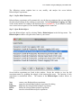


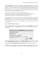

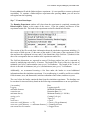

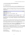

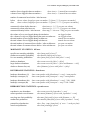


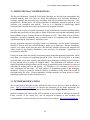


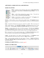

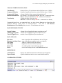


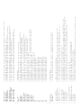


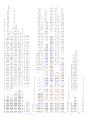




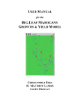


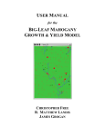
![(TXDOL]HU ,, and (TXDOL]HU ' User Guide Please Read First](http://vs1.manualzilla.com/store/data/006869043_1-f0643d0d39fcf451fb31bcf674da5fa3-150x150.png)