1
Cell Illustrator™: User Guide © 2002-2010 Human Genome Center, Institute of Medical Science, The University of Tokyo All rights reserved. TABLE OF CONTENTS: 1 INTRODUCTION............................................................................................5 2 GETTING STARTED......................................................................................6 2.1 Cell Illustrator Online ..................................................................................6 2.2 Run Cell Illustrator Online (CIO)..................................................................6 2.3 Licensing Information...................................................................................7 2.4 CI Memory Customization...........................................................................8 3 CELL ILLUSTRATOR ELEMENTS...............................................................9 3.1 Concept Overview........................................................................................9 3.2 Entities.......................................................................................................10 3.3 Connectors.................................................................................................11 3.4 Processes..................................................................................................12 3.5 Element Combinations ..............................................................................13 3.6 Discrete Elements Example 1....................................................................15 3.7 Discrete Elements Example 2: Connector Speed.....................................16 3.8 Continuous Elements Example 1..............................................................17 3.9 Continuous Elements Example 2..............................................................19 4 BIOLOGICAL PROCESS MODELING WITH CELL ILLUSTRATOR.........21 4.1 Degradation...............................................................................................21 4.2 Translocation.............................................................................................23 4.3 Transcription..............................................................................................24 4.4 Complex.....................................................................................................26 4.5 Tetramerization..........................................................................................28 4.6 Stochastic Tetramerization........................................................................29 4.7 Custom Tetramerization............................................................................30 4.8 Separation..................................................................................................31 4.9 Inhibition.....................................................................................................33 4.10 Catalysis..................................................................................................35 5 CELL ILLUSTRATOR USER INTERFACE AND MODEL CREATION......38 5.1 Add Elements.............................................................................................38 5.2 Modify a Model ..........................................................................................39 5.3 Change Element Properties ....................................................................40 5.4 Element Settings Frame and Element Lists Frame...................................41 5.5 Biological Elements and Pathway Fragments...........................................48 5.6 Script Editor...............................................................................................55 5.7 Preferences Frame....................................................................................58 5.8 Graph Layout Frame..................................................................................59 6 SIMULATION................................................................................................60 6.1 Simulation Concept....................................................................................60 © 2002-20 Human Genome Center, Institute of Medical Science, The University of Tokyo. All rights reserved. Page 2 of 88 6.2 How to Set Up and Run Simulation...........................................................62 6.3 Viewing and Analyzing Simulation Results................................................67 6.4 Running SECG Simulation........................................................................68 7 TOOLS FOR MODEL ANALYSIS................................................................72 7.1 Navigator....................................................................................................72 7.2 Finder.........................................................................................................73 7.3 Print and Print Area...................................................................................74 7.4 Export Options...........................................................................................74 8 MAKING COMPLEX MODELS....................................................................75 8.1 Grouping and Ungrouping.........................................................................75 8.2 Import of CellML or SBML models.............................................................76 8.3 Import of CSO and BioPAX models...........................................................76 9 CELL ILLUSTRATOR PLAYER..................................................................77 APPENDIX A: TUTORIAL—MODELING FAS LIGAND INDUCED APOPTOSIS.................79 APPENDIX B: USING DIFFERENTIAL EQUATIONS IN CI.........................86 APPENDIX C: KINETIC STYLES..................................................................88 CI REFERENCES...........................................................................................90 © 2002-20 Human Genome Center, Institute of Medical Science, The University of Tokyo. All rights reserved. Page 3 of 88 1 Introduction Cell Illustrator™ (CI) is a software tool that enables biologists to model, elucidate and simulate complex biological processes and systems [11]. It allows researchers to model metabolic pathways, signal transduction cascades, gene regulatory pathways as well as dynamic interactions of various biological entities such as genomic DNA, mRNA and proteins. Cell Illustrator models are used to visualize biopathways, interpret experimental data and test hypotheses. In addition, it provides researchers with model diagrams of publication quality and simulation result charts. Cell Illustrator has been successfully utilized to model biological pathways like Circadian Rhythms of Drosophila, Glycolytic pathway and Fas ligand induced Apoptosis [1, 2, 3, 4, 5, 6, and 7]. Using the graphical user interface of Cell Illustrator, researchers can create and simulate their own molecular pathway models. Some of the key features of Cell Illustrator are: (a) Pathway construction and visualization—construct models graphically by drag and drop entities that represent bio-components in the biological pathways; (b) Pathways simulation—specify mathematical formulas for biochemical reactions in the pathway for simulation; The simulation can be run inside the workspace window in an interactive mode, or sent to a remote server (Cell Illustrator Server) (c) Simulation replay – the simulation results can be logged and then visualized and analyzed in Cell Illustrator Player; (d) Simulation animation—Cell Illustrator’s simulation results can be edited into an animation script file and then be used as the input to Cell Animator—a module that produces high quality presentation of the studied mechanism’s dynamic behavior; (e) Model import - previously created models or sub-models can be imported from SBML, CellML files or from public or proprietary libraries and databases like KEGG [9,12]. The documentation for the Cell Illustrator software includes the manuals listed below: Cell Illustrator User Manual: Introduction to Cell Illustrator system Cell Illustrator Reference Manual: Detailed description of Cell Illustrator functionalities Cell Illustrator Player Reference Manual: Detailed description of Cell Illustrator Player functionalities This manual describes version 5.0 of Cell Illustrator Online (CIO5.0). © 2002-20 Human Genome Center, Institute of Medical Science, The University of Tokyo. All rights reserved. Page 4 of 88 2 Getting Started 2.1 Cell Illustrator Online Cell Illustrator is available as a Java Web Start application – CI Online. CI Online can be run directly from the website, without the need to install software on local computer. CI Online is a client-server solution that enables the user to create, manipulate and simulate bio-pathway models locally within CI workspace and to store and organize them on the remote CI Online Server. Additionally CI Online Server gives the user convenient access to libraries and databases of bio-pathway models. 2.2 Run Cell Illustrator Online (CIO) In order to run Cell Illustrator correctly, Java version j2sdk 1.5.0 or higher needs to be installed. Java Runtime Environments (JREs) are available for download at: http://java.sun.com/downloads. To run Cell Illustrator Online: - Open the Cell Illustrator Online website at https://cio.bioillustrator.com or https://cionline.hgc.jp in your web browser - Register to obtain the CI Online account - Run Cell Illustrator © 2002-20 Human Genome Center, Institute of Medical Science, The University of Tokyo. All rights reserved. Page 5 of 88 - In the CI Startup frame, enter the login data that you obtained during the registration and press Sign In Note: It is recommended to select the Remember Password option. After a successful login, the login and password will be stored on your local computer and you will not need to enter the login data again. - After this CI Online is downloaded from the server. This may take several minutes. CI Online is a client-server solution that enables the user to create, manipulate and simulate bio-pathway models locally within CI workspace and to store and organize them on the remote CI Online Server. Additionally CI Online gives the user convenient access to libraries and databases of bio-pathway models. In CI Online, Cell Illustrator is the front-end, where the user prepares a pathway and simulates it. The Cell Illustrator client communicates with the CI Online Server over the internet (HTTP or HTTPS protocol). The CI Online Server is a place where the user logs-in to store and manage his pathways and to share them with other users. 2.3 Licensing Information To run Cell Illustrator, you need to obtain a CI Online account. For details, please contact your local Cell Illustrator reseller. CI offers several license types: Professional, Standard, Classroom, Access and Player. The main differences between the license types are in the simulation capabilities of CI and are briefly summarized at https://www.cellillustrator.com/lineup. Note: This manual describes all functions available in the CI (CI Professional license type). A given function described in this manual might be disabled or not available in the limited versions CI Access and CI Player. © 2002-20 Human Genome Center, Institute of Medical Science, The University of Tokyo. All rights reserved. Page 6 of 88 2.4 CI Memory Customization When starting CI Online, you can set the maximum memory for Cell Illustrator in the Login dialog box. © 2002-20 Human Genome Center, Institute of Medical Science, The University of Tokyo. All rights reserved. Page 7 of 88 3 Cell Illustrator elements CI is designed to model biological pathways using three types of abstractions: entities, processes and connectors. 3.1 Concept Overview The modeling and simulation engine of Cell Illustrator™ is based on an extension of the Petri-net methodology. A Petri-net models a system of conditions and instantaneous events, their dependencies and mutual synchronization. The Hybrid Petri-net with extensions (HFPNe) employed in the Cell Illustrator adds the notion of continuous and generic processes and quantities, which are essential to the description of biological systems [10]. The following table presents a summary of the Petri-net model elements, their explanations and equivalent biological meanings. Table 1 HFPNe elements. Hybrid Functional Petri Net Elements Petri Net Component Symbol Biological Equivalent Discrete Entity A countable biological component or event that is quantified or represented by an integer, e.g. the number of molecules locating at the membrane, an event that describes whether a protein is binding to DNA or not. Discrete Place A discrete place holds tokens represented as a non negative integer. Quantity The number of entity items present, e.g. the number of molecules binding to DNA, ON/OFF state of a gene expression, etc. Tokens A token is a unit held in a place. Discrete Transition Discrete Process A discrete transition is a discrete process that consumes tokens from their input places and produces tokens into their output places. The input and output places are connected to a transition by arcs. A transition “fires” and the process is invoked if all the conditions for firing are met. Every transition has a delay time for firing. A biological reaction that converts quantities in discrete entities into quantities in other discrete entities. A switching mechanism can be also handled as a discrete process which receives some signals and sends out signals for a pathway. Continuous Entity Continuous Place A biological entity like a concentration of a protein, enzyme, or ion, etc. the quantity of which can be represented as a real number. A continuous place holds a non negative real number. Marking A variable representing the state of a place. © 2002-20 Human Genome Center, Institute of Medical Science, The University of Tokyo. All rights reserved. Concentration, Quantity m System status representing quantity or concentration of proteins, enzymes and ions. Page 8 of 88 Continuous Transition Continuous Process A continuous transition is a continuous process consuming quantities of its input places and producing quantities into its output places. It defines a continuous flow that is specified by a speed of firing [v]. A biological process or a reaction like transcription, translation, or enzymatic reaction, which consumes some entities’ (inputs) quantity and produces others (output), according to a rate formula. Generic Entity Universal Place A universal place can handle a list of variables of various types (double, Boolean, string, etc.). A biological/chemical/physical entity that is not pre-defined. May contain more data types like string that is used to represent DNA sequence. Universal transition Generic Process A transition for a universal place. A universal transition allows the arcs connecting with this transition to use their functions (firing speeds). A complicated biological/chemical/ physical process, e.g., a translation process. Arc/Connector Normal Arc A directed arc. Connects a transition to a place or connects a place to a transition. An arc has a weight. Inhibitory Arc Connects a place to a transition. An inhibitory arc disables a transition. If the quantity in its source place is greater than the weight of the arc, the transition cannot fire. Process Connector Connects input entities to a process and process to output entities. Its weight parameter specifies an activation threshold. Process Connector allows quantities flow in the model. Inhibitory Connector Prevents a process from being activated. Inhibitory Connector facilitates the modeling of the inhibition/competition process. Association Connector Test Arc Connects a place to a transition. A test arc does not consume any quantity of the source place by firing. 3.2 Connects entities without causing concentration change. Defines which entities are associated with each other, but not as inputs or outputs. Association Connector allows the modeling of enzymatic reactions as well as other catalytic processes. Entities Entities are abstract elements that can represent any type of biological concepts like mRNAs, DNA, proteins, ligands, and compounds. They can also represent cellular structures like mitochondria, cell nuclei, cells or biological phenomena like transcription and translation. An entity (Figure 1) contains a value which is interpreted as its quantity or concentration. You can input a more meaningful name and value for the entity. Also, each entity has an associated variable (e1, e2, e3) representing its quantity (30, 123.2, ATGC, respectively). The mathematical equations used for simulation are expressed in terms of these variables. © 2002-20 Human Genome Center, Institute of Medical Science, The University of Tokyo. All rights reserved. Page 9 of 88 There are three types of entities: discrete entity, continuous entity and generic entity. Figure 1 Discrete entity holds an integer quantity (Integer or Long). In contrast, a continuous entity has a continuous (e.g. real / fractional) number as its quantity (Double). This type of entity is used to represent concentrations, e.g. the number of ions or enzymes. Other type of entity is a generic entity. It holds string or logical value (String or Boolean). 3.3 Connectors Connectors are used to connect entities to processes (input connectors) or processes to entities (output connectors). There are three types of connectors (Figure 2): process connectors, inhibitory connectors and association connectors. An input connector can take all three types. In contrast, an output connector is always of the process type. Correspondingly, all types of connectors can connect input entities to a process. In contrast, only a process connector can connect a process to an output entity. Figure 2 The threshold is an input connector’s parameter. It can be a value or a script, e.g. m/10. This parameter is used to define the minimum value of the input entities needed for the activation or deactivation of the linking processes. A process and an association connector become activated if the threshold of the connector is smaller than the value of input entity. On the other hand, inhibitory connectors are activated when input entity is less than this threshold. Inhibitory connectors are used to model repression (see Section 4.9). Association connectors are used to model the situation when entities and processes need to be linked together, but nothing is produced or consumed. They do not allow transport of quantities. They are used when the input entities concentrations do not change (see Section 4.10). © 2002-20 Human Genome Center, Institute of Medical Science, The University of Tokyo. All rights reserved. Page 10 of 88 3.4 Processes Processes (Figure 3) define the rate of entity value changes and interactions among entities. Processes are used to model biological reactions such as enzymatic reactions or protein complex formation processes. Processes can take multiple inputs (e.g. consume different entities to produce new entities) and have multiple outputs (e.g. produce different entities, such as breaking down sacharose into glucose and fructose). Also, like entities, processes can be continuous (continuous processes), discrete (discrete processes) or generic (generic processes), depending on the input, output and timing. Only generic processes are able to handle generic entities. Figure 3 In general terms, if all input connectors of a process are activated the process is said to be enabled (see Section 6.1). When a process is enabled, the reaction that it represents will fire (will be executed) immediately or after a certain time interval. This will cause a change in value for all connected entities. For example, if a process represents the reaction of a protein precursor which turns into an activated protein by phosphorylation, the decrease of the precursor protein and the increase of the active protein on account of the speed of phosphorylation is simulated once the process fires. The exact conditions for enabling a process depend on its Firing Style parameter and are described in detail, along with other process parameters, in Section 5.4.2. The process type determines its calculation style. The continuous process has the speed calculation style - the process calculates the speed of production or consumption of the entities. On the other hand, the discrete process has the add style - the process calculates the concrete values that should be added/subtracted to the entities. Finally, the calculation style of the generic process is update, i.e., the process calculates a concrete value that will replace the entity value. The Kinetic Script parameter specifies how to calculate the value change of connected entities in each of the three cases. See the Reference Manual for details. Each discrete and generic process has an additional Delay parameter that can be a constant or a function. The firing of a discrete process occurs abruptly with the delay associated with the process. The same applies to generic processes. The activity of continuous processes is different: The firing of a continuous process occurs continuously. Consequently, a continuous process does not hold the Delay parameter. © 2002-20 Human Genome Center, Institute of Medical Science, The University of Tokyo. All rights reserved. Page 11 of 88 To employ generic processes one must use the Pnuts scripting language. Use of Pnuts is briefly described in Section 5.6. Another important parameter associated with a process is its Kinetic Style. If the process kinetic style is Custom then the value change after the process fires is the same for all connected input/output entities. For all other kinetic styles, the value change at each entity depends on connector-specific parameters such as Connector Stoichiometry and Connector Speed. Thus, it may be different for different input/output entities. 3.5 Element Combinations All combinations of discrete and continuous CI elements are presented in Table 2 and Table 3. Table 2 Output Connectors Transport quantity v(t) through the Connector at d(t) intervals. Not Allowed. Transport quantity v(t) through the Connector at each d(t) interval. Sequentially transport quantity v(t) through the Connector. Not Allowed. The variable m(t) represents quantity or concentration of the entity at time t. The variable w(t) is the threshold of the corresponding connector. The constant d(t) is the delay time of the corresponding process and the function v(t) is the speed of the corresponding process at the time t. Note that CI checks and prohibits the connections that are not allowed during model creation. © 2002-20 Human Genome Center, Institute of Medical Science, The University of Tokyo. All rights reserved. Page 12 of 88 Table 3 Input Connectors Process is enabled at intervals of the time d(t) while m(t)>w(t) holds. Not Allowed Process is enabled at intervals of the time d(t) while m(t)>w(t) holds. Process is enabled at the speed of v(t) while m(t)>w(t) holds. Process is enabled at intervals of the time d(t) while m(t)>w(t) holds, but no quantity change. Process is enabled while m(t)>w(t) holds, but no quantity change. Process is enabled at intervals of the time d(t) while m(t)>w(t) holds, but no quantity change. Process is enabled while m(t)>w(t) holds, but no quantity change. Process is not enabled while m(t)>w(t) holds. Process is not enabled while m(t)>w(t) holds. Process is not enabled while m(t)>w(t) holds. Process is not enabled while m(t)>w(t) holds. 3.6 Discrete Elements Example 1 Figure 4 The model in Figure 4 consists of two discrete entities e1 and e2, and the discrete process p1 between them. The entity e1 is connected to p1 with the input process connector c1. The process p1 is connected to e2 with the output connector c2. The kinetic style of the process is Custom. The entities e1 and e2 have the initial value 10 and 0, respectively. The input connector c1 has the Threshold parameter equal 2. The threshold of an input connector controls the activity of process p1. The process p1 has the delay parameter equal 1 and the add parameter equal 2. This model can be used for auto catalytic reactions, e.g. protein auto-phosphorylation. © 2002-20 Human Genome Center, Institute of Medical Science, The University of Tokyo. All rights reserved. Page 13 of 88 In the HFPNe theory, time is measured in virtual time units called Petri net time (pt). At time 0, the value of e1 is 10 and the threshold of c1 is 2, and the process p1 is enabled. When all input processes are enabled, the connected discrete process is really executed after the delay time of the process. In this example, the delay parameter of the process p1 is 1. Therefore, the process is executed at time 1. Consequently, at time 1 the entity e1 decreases and e2 increases by the speed of process p1, i.e., 2. Thus, at time 1, the value of entity e1 and e2 becomes 8 and 2, respectively. At time 4, the value of the entity e1 becomes 2 and the process p1 cannot be enabled because the value of e1 is less or equal than the threshold of c1. At that time, the process p1 cannot be enabled and e1 and e2 reach a stable state. The results of the simulation are presented below (Figure 5). Figure 5 3.7 Discrete Elements Example 2: Connector Speed In the previous model, the values of e1 and e2 increase and decrease by the same amount (2) at each time interval because their value depends on the add value of the process p1. However, modeling differing increase and decrease in the value of connected entities is sometimes necessary, e.g., when a monomer becomes a dimer or a trimer and vice versa. To deal with this type of process, set the process kinetic style to connector custom and then define the value changes of the connected entities separately. Figure 6 © 2002-20 Human Genome Center, Institute of Medical Science, The University of Tokyo. All rights reserved. Page 14 of 88 The example in Figure 6 demonstrates the use of the connector custom kinetic style. The difference between the previous example and the model in Figure 6 is as follows: (i) The add parameters of connector c1 and c2 are 2 and 1, respectively. At time 0, the value of e1 is 10 and the threshold of c1 is 1 and the process p1 is enabled. After the delay of p1, i.e. 1, the process is executed. The add value of c1 and c2 are 2 and 1, respectively. Thus, the value of e1 and e2 becomes 8 and 1 at time 1, respectively. At time 4, the value of e1 and e2 are 2 and 4, respectively. At that time, the process p1 is not enabled and e1 and e2 reach a stable state. The results of the simulation are presented below (Figure 7). Figure 7 3.8 Continuous Elements Example 1 In the previous two examples, discrete entities and discrete processes have been used. However, in many cases, entity values should be treated as continuous variables rather than discrete variables. The model in Figure 8 has been created by conversion of the discrete model in Section 3.6. Figure 8 More specifically, the differences between the models in Figure 4 and in Figure 8 are as follows: Step 1: The type of entities e1 and e2 is changed from discrete to continuous. Step 2: The type of process p1 is changed from discrete to continuous. Step 2: The delay of process p1 is changed from 1 to 0. © 2002-20 Human Genome Center, Institute of Medical Science, The University of Tokyo. All rights reserved. Page 15 of 88 All other parameters are the same as in the discrete model in Section 3.6. As described in Section 3.6, the threshold parameter of the input connector works like the threshold of the activity of process p1. In this example, at time 0, the value of e1 is 10 and the threshold of c1 is 2 and the process is enabled. When all input connectors are enabled, the connected continuous process is executed with no delay. Since p1 is connected to e1 with the quantity m1, and its output is connected to e2 with the quantity m2, the equations for quantities change are: − dm1 dm2 = =1 dt dt At time 4, the value of e1 is the same as the threshold of c1, i.e. 2. At that time, the process p1 cannot be enabled and e1 and e2 reach a stable state. The results of the simulation are presented below (Figure 9). Figure 9 The same conversion process can be applied to the discrete model in Section 3.7 (Figure 10). Figure 10 The equations for quantity changes are: − dm1 dm2 = 2, =1 dt dt The results of the simulation are presented below (Figure 11). © 2002-20 Human Genome Center, Institute of Medical Science, The University of Tokyo. All rights reserved. Page 16 of 88 Figure 11 3.9 Continuous Elements Example 2 In the previous two examples, discrete examples were converted into similar models with continuous elements. For kinetic based modeling, one should use a continuous model rather than a discrete one. In the following model (Figure 12), the consumption ratio of e1 is proportional to the value of e1, i.e. the speed of process p1 follows the mass action kinetics. Figure 12 The difference between the present model and the model in Section 3.8 is that the speed of p1 is changed from 1 to 0.05*m1. In this model, process p1 continuously transports entity e1 to e2 at the rate of 1/20 of e1’s concentration m1. Since p1 is connected to e1 with quantity represented by m1, and its output is connected to e2 with quantity m2, the equations for quantities change are: − dm1 dm2 = = 0.05 * m1 dt dt The value of entity e1, i.e. m1, decreases while the value of entity e2, i.e. m2, increases during simulation. The equation (0.05*m1) of process p1 governs this change of value per unit time (see Section 6.1 for Simulation Details). The results of the simulation are presented below (Figure 13). © 2002-20 Human Genome Center, Institute of Medical Science, The University of Tokyo. All rights reserved. Page 17 of 88 Figure 13 If consumption and generation speed should be different, the Connector Custom kinetic style should be used and the corresponding speed/add parameters for connectors c1 and c2 should be set. In Figure 14, the speed of c1 and c2 is 0.05*m1 and 0.1*m1, respectively. Figure 14 The results of the simulation are presented below (Figure 15). Figure 15 © 2002-20 Human Genome Center, Institute of Medical Science, The University of Tokyo. All rights reserved. Page 18 of 88 4 Biological Process Modeling with Cell Illustrator This section briefly explains how to simulate major biological processes with CI. The examples have been designed to help the novice user to become familiar with the Hybrid Petri Net modeling method and notation. 4.1 Degradation In a cell, nearly all mRNAs and proteins fragment into parts at certain speeds. This fragmentation activity is called degradation. A model of degradation can be created with the following steps. Step1: Create an entity and change its name, e.g. p53, and set its value, e.g. 10. Step2: Create a process and set its name, e.g. “degradation”. Step3: Connect the p53 entity to the degradation process with the process connector. Step4: Set the degradation speed by editing the Kinetic Script parameter of the degradation process. For the discrete process the default speed is 1.0. For the continuous process, set the Kinetic Style to Custom and then edit the Kinetic Script (speed). In Step1 and Step2 the following combinations are possible (Figure 16): a discrete entity and a discrete process, a continuous entity and a continuous process, a continuous entity and discrete process Figure 16 The results of the simulation are presented below (Figure 17). © 2002-20 Human Genome Center, Institute of Medical Science, The University of Tokyo. All rights reserved. Page 19 of 88 Figure 17 If the degradation speed depends on the value of p53 protein (say m), in Step 4 the speed should be made dependent on m (Figure 18). Figure 18 The results of the simulation are presented below (Figure 19). Figure 19 © 2002-20 Human Genome Center, Institute of Medical Science, The University of Tokyo. All rights reserved. Page 20 of 88 4.2 Translocation In a cell, mRNA and proteins move from one compartment to others, e.g. from nuclei to cytoplasm and vice versa. A model for this can be created with the following steps. Step1: Create two entities and change their names, e.g. p53_nuclei and p53_cytoplasm and set their values, e.g. 100 and 0. Step2: Create a process and set its name, e.g. translocation. Connect the p53_nuclei to the process and connect the process to p53_cytoplasm. Step3: Set the translocation speed by editing the Kinetic Script parameter of the translocation process. For the discrete process the default speed is 1.0. For the continuous process, set the Kinetic Style to Custom and then edit the Kinetic Script (speed). In Step1 and Step2, possible combinations of (p53_nuclei, translocation, p53_cytoplasm) triple are (discrete, discrete, discrete), (discrete, discrete, continuous), (continuous, discrete, continuous), (continuous, discrete, discrete) and (continuous, continuous, continuous) (Figure 20). Figure 20 The simulation results of the discrete model are presented below (Figure 21). © 2002-20 Human Genome Center, Institute of Medical Science, The University of Tokyo. All rights reserved. Page 21 of 88 Figure 21 If the translocation speed depends on the quantity of p53_nuclei (say m1), as in the degradation example, Section 4.1, the process speed should be made dependent on m1/10 in Step3. (The factor of 1/10 was used in the example in Figure 22.) Figure 22 The results of the simulation are presented below (Figure 23). Figure 23 4.3 Transcription Transcription modeling can easily be done using CI. A model can be created with the following steps. Step1: Create a process and set its name, e.g. transcription. Step2: Create an entity and change its name, e.g. mRNA_p53. © 2002-20 Human Genome Center, Institute of Medical Science, The University of Tokyo. All rights reserved. Page 22 of 88 Step3: Connect the transcription process to mRNA_p53 entity with the process connector. Step4: Set the transcription speed by editing the Kinetic Script option of the transcription process. For the discrete process the default speed is 1.0. For the continuous process, set the Kinetic Style to Custom and then edit the Kinetic Script (speed). In Step1 and Step2, possible combinations of the pair (transcription, mRNA_p53) are (discrete, discrete), (discrete, continuous) and (continuous, continuous) (Figure 24). Cell Illustrator facilitates the modeling of the path DNA mRNA Protein not only as a concentration function of DNA, mRNA and Protein. Global transcription and translation mechanism can be established with a string input (DNA sequence), intermediate product (proper mRNA) and product (Protein). This mechanism can produce simultaneously many proteins from different DNA sequences. Figure 24 The simulation results of the discrete model the are presented below (Figure 25). Figure 25 Normally, mRNA synthesis is associated with its degradation. The models presented below (Figure 26) combine the transcription process with the degradation process in Section 4.1 (The same speed m/10 is applied.) © 2002-20 Human Genome Center, Institute of Medical Science, The University of Tokyo. All rights reserved. Page 23 of 88 Figure 26 The results of the simulation are presented below (Figure 27). Figure 27 4.4 Complex In a cell, a set of proteins binds and creates a complex. A model for this can be created with the following steps. Step1: Create three entities and set their names, e.g. p53, mdm2, p53_mdm2, and set their values, e.g. 100, 50, 0. Step2: Create one process and changes its name, e.g. complex. Step3: Connect p53 entity and mdm2 entity to the complex process. Connect the combine process to the p53_mdm2 entity. Step4: Set the combine speed by editing Kinetic Style and Kinetic Script options to values Custom and 1.0. In Step1 and Step2, 9 combinations of element types in the pattern (p53, mdm2, p53_mdm2, complex process) are allowable, i.e., (discrete or continuous, discrete or continuous, discrete or continuous, discrete) and (continuous, continuous, continuous, continuous) (Figure 28). © 2002-20 Human Genome Center, Institute of Medical Science, The University of Tokyo. All rights reserved. Page 24 of 88 Figure 28 The simulation results of the continuous model are presented below (Figure 29). Figure 29 If the complex speed strictly depends on the value of p53 (m1) and mdm2 (m2), the speed of the complex process needs to be (m1*m2)/400 (the factor 1/400 is © 2002-20 Human Genome Center, Institute of Medical Science, The University of Tokyo. All rights reserved. Page 25 of 88 an example) for the model where all elements are of the continuous type as in Figure 30. Figure 30 The results of the simulation are presented below (Figure 31). Figure 31 4.5 Tetramerization In a cell, some proteins create a self-complex under certain conditions. For example, p53 can create a homotetramer. The process of creating tetramers is called tetramerization. The three examples below show how various kinetic styles processes can be used for the modeling of tetramerization. The speed of tetramerization is linearly dependent on the mass of monomers in the first example. In the second example, stochastic perturbation is introduced. Finally, in the most advanced example, tetramization is defined by a script. A simple model of tetramerization can be created using the following steps: Step 1: Create two entities and set their names, e.g. p53 (monomer) and p53 (tetramer). Set the initial value of the monomer to 10. Step 2: Create a process and set its name, e.g. “tetramerization”. Step 3: Connect the p53 (monomer) entity to the process with a process connector. © 2002-20 Human Genome Center, Institute of Medical Science, The University of Tokyo. All rights reserved. Page 26 of 88 Step 4: Connect the process to the p53 (tetramer) entity with a process connector. Step 5: Set the Kinetic Style of the process to Mass and set c1 Stoichiometry to 4. Leave the default values for the other parameters of the process: Coefficient1 0.01, Coefficient2 - 0.1 and c2 Stoichiometry - 1. Figure 32 With the model, as in Figure 32, the speed of the tetramerization process depends on the value of p53 (tetramer). To make the process of tetramerization faster the Coefficient1 value should be increased. To change tetramerization into the dimerization process the “c1 stoichiometry” value should be changed to 2. More details on parameters related to the Mass kinetic style can be found in the section . 3.4 Processes. The results of the simulation are presented below (Figure 33). Figure 33 4.6 Stochastic Tetramerization Normal biological processes (e.g. dimerization or tetramerization) are not deterministic but stochastic. To improve modeling of the biological processes one can use the Stochastic Mass kinetic style of the process. Starting from the previous model, the stochastic tetramerization process can be modeled as follows: Step 6: Change the Kinetic Style of the process to Stochastic Mass. Set the Standard Deviation to 0.2. This parameter controls the distribution of the randomly generated process speed. © 2002-20 Human Genome Center, Institute of Medical Science, The University of Tokyo. All rights reserved. Page 27 of 88 Step 7: Make sure that other parameters are the same as in the previous Tetramerization example, i.e. c1 Stoichiometry is 4. Figure 34 In the model, shown in Figure 34, the speed of the tetramerization process represents stochastic behavior. Parameters related to Stochastic Mass kinetic style are described in section 3.4 Processes. The example results of the simulation are presented below (Figure 35). Note that subsequent simulation runs will give different results due to the stochastic nature of the model. Figure 35 4.7 Custom Tetramerization Tetramerization can also be defined by a custom formula: In the example in Section 4.5, the process speed depends on the p53 (monomer) in a linear way, but one can change it into a quadratic function by writing a script. The example in 4.5 could be modified as follows: Step 6: Change the Kinetic Style of the process to Connector Rate and set the Rate parameter as 0.001*m1*m1. Step 7: Make sure that other parameters are the same as in the previous Tetramerization example, i.e. c1 Stoichiometry is 4. © 2002-20 Human Genome Center, Institute of Medical Science, The University of Tokyo. All rights reserved. Page 28 of 88 Figure 36 In the model in Figure 36, the speed of the tetramerization process is proportional to the square of p53 (monomer). The results of the simulation are presented below (Figure 37). Figure 37 4.8 Separation In a cell, binding proteins are sometimes separated with proteins. A model can be created here with the following steps: Step1: Create three entities and set their names, e.g. p53, mdm2, p53_mdm2, and set their value, e.g. 50, 0, 50. Step2: Create one process and set its name, e.g. separate. Step3: Connect the p53_mdm2 entity to the separate process. Connect the separate process to the p53 entity and the mdm2 entity. Step4: Set the separate speed by editing Kinetic Style and Kinetic Script options to values Custom and 1.0. Again, 9 combinations of element types in the set (p53, mdm2, p53_mdm2, separate process) are possible in Step1 and Step2, i.e. (discrete or continuous, discrete or continuous, discrete or continuous, discrete) and (continuous, continuous, continuous, continuous) as in Figure 38. © 2002-20 Human Genome Center, Institute of Medical Science, The University of Tokyo. All rights reserved. Page 29 of 88 Figure 38 The results of the simulation are presented below (Figure 39). Figure 39 If the speed of the separate process strictly depends on the value of p53_mdm2 (say m1), this can be expressed by a respective equation defining the speed parameter of the process (In Figure 40, m3/20 for the model where all elements are of the continuous type). © 2002-20 Human Genome Center, Institute of Medical Science, The University of Tokyo. All rights reserved. Page 30 of 88 Figure 40 The results of the simulation are presented below (Figure 41). Figure 41 For models based on discrete elements, it is difficult to create a model that fulfills this condition. 4.9 Inhibition A specific drug sometimes inhibits activities of transcription. The transcription model in Section 4.3 is modified with an inhibitor activity as follows. Step1: Create an entity and set its name, e.g. doxorubicine. Step2: Create a process and connect it to the doxorubicine entity with the process connector. Step3: Connect the doxorubicine entity to the transcription process with the inhibitory connector. Step4: Do not change the threshold of the inhibitory connector (the default value is 0). The type of the doxorubicine entity can be either discrete or continuous. With the model in Figure 42, one can simulate the situation where the concentration of doxorubicine is growing. If the inhibition connector threshold is set to 0 for continuous processes the translation will be stopped immediately after the first Sampling Interval. For a discrete process Translation will be stopped after the first step, as during the first step process (p1) is enabled. © 2002-20 Human Genome Center, Institute of Medical Science, The University of Tokyo. All rights reserved. Page 31 of 88 Figure 42 The results of the simulation are presented below (Figure 43) Figure 43 If the threshold of the inhibitory connector is modified to 5 (Figure 44) the results will be different. The results of the simulation are presented below (Figure 45) Figure 44 © 2002-20 Human Genome Center, Institute of Medical Science, The University of Tokyo. All rights reserved. Page 32 of 88 Figure 45 As in Figure 43 and Figure 45, if doxorubicine is treated the transcription of p53 is inhibited. The inhibitory activity will be adjusted with the threshold of the inhibitory connector. 4.10 Catalysis Enzymes catalyze a variety of chemical reactions. The model of an enzymatic reaction can be created with the following steps. The first three steps are similar to the translocation process in Section 4.2. Step1: Create two entities and change their names, e.g. p53 and p53-P and set their values, e.g. 10 and 0. Step2: Create a process and set its name, e.g. catalysis. Connect p53 to the process and connect the process to p53-P. Step3: Set the catalysis speed by editing the speed option of the catalysis process. Set Kinetic Style to Custom and Kinetic Script (speed) to 1.0. Step4: Create one entity and change its name, e.g. CAK. Step5: Create a process and connect it to the CAK entity with the process connector. Set kinetic style to Custom and kinetic script (speed) to 1.0. Step6: Connect the CAK entity to the catalysis process with the association connector. Step7: Change the threshold of the association connector to 1(the default value is 0). The type of CAK entity is continuous. With the model in Figure 46, one can simulate the situation where CAK (enzyme) concentration is growing. If the association connector threshold is set to 1 the catalysis process will be enabled when the CAK entity value reaches 1 level. © 2002-20 Human Genome Center, Institute of Medical Science, The University of Tokyo. All rights reserved. Page 33 of 88 Figure 46 The results of the simulation are presented below (Figure 47) Figure 47 If the threshold of the association connector is modified to 5 (Figure 48) the results will be different. The results of the simulation are presented below (Figure 49) Figure 48 © 2002-20 Human Genome Center, Institute of Medical Science, The University of Tokyo. All rights reserved. Page 34 of 88 Figure 49 In the presented reaction, CAK influence on the model is enabling/disabling the reaction. The CAK activity will be adjusted with the threshold of the association connector. However, in most of the systems, the reaction rate depends on enzyme concentration and substrate concentration. In the example in Figure 50, the speed of the catalysis process is defined with the equation (m1*m2)/10. The model is made of continuous type elements and the threshold of association connector is reset to 0. Figure 50 The results of the simulation are presented below (Figure 51). Figure 51 © 2002-20 Human Genome Center, Institute of Medical Science, The University of Tokyo. All rights reserved. Page 35 of 88 5 Cell Illustrator User Interface and Model Creation At Cell Illustrator startup, a single main window pops up. You can create, open, save and print a biological pathway model file using options in the File menu (Figure 52). This window has the Menu Bar at the top that allows you to manipulate the model diagram. Figure 52 To create a new model, the first step is to open an empty canvas window for the model, which can be accomplished by either: 1. clicking on the top icon in the left toolbar 2. clicking on the File in the Menu Bar and selecting the “New” option 5.1 Add Elements To add a new element—an entity or a process, select one of , , , , and icons from the top toolbar, and then click on the canvas workspace where you want to place it. You may continue and place more components of the selected type on the canvas. Alternatively, you can press the right mouse button anywhere on the canvas and choose the desired element from the popup menu using Insert Entity/Insert Process function. The new element will be placed at the center of the active canvas. Lastly, you can select a predefined element in the Biological Elements frame (see Section 5.5.1). Each entity has three labels associated with it for you to edit by double clicking (see Figure 1). On the upper left is the Name of the entity for associating biological concepts with the entity. The upper right label is the Variable representing this entity. It is used in mathematical equations to define the rate of reaction in the model. The lower left label represents the current value of the entity. You can edit it © 2002-20 Human Genome Center, Institute of Medical Science, The University of Tokyo. All rights reserved. Page 36 of 88 to enter the initial value for the selected entity. Note that for discrete entities, this value must be an integer. A process can have up to four associated labels (see Figure 3). At the upper left is the Name of the process. The lower right label is the Kinetic Script of the process. The upper right label is the Firing Style of the process and the lower left label is the Delay of the process. To add a connector to link two elements, select a connector type from , and icons in the Draw toolbar above the canvas pane and then click on the element where the connection originates. Next, click on the element you want to connect to. The connector will be automatically drawn to connect the two elements. Note that a connector links entities to processes, not entities to entities or processes to processes. If you draw a connector between two entities, a process with default parameters is inserted between them. Also, discrete entities cannot connect to continuous processes (see Element Combinations in Section 3.5). Generic entities can only connect to generic processes. Each connector has up to three labels: above the connector is its name, below is its firing style, and below the connector is its threshold (if threshold firing style is enabled) or the rule (if rule firing style is enabled) (see Figure 2). The threshold is a minimum value for the activation of the connector (see Simulation Concept, Section 6.1). 5.2 Modify a Model The user can move any element within the model (i.e., change its location). To carry out this task, click on the Selection Mode button from the Draw toolbar. Then, click on the element in the canvas and drag it to move it. You can also drag the mouse to select multiple elements and then right click the mouse to bring up a popup menu which allows to you to arrange, copy, cut, duplicate or delete the selected elements. A mouse right click on a selected single element will bring up a customized popup menu with additional options to modify the element. The Draw and Element toolbars contain buttons for frequently performed editing operations. This includes: • • • “Insert Frame”— Create a background frame. “Insert Text” — Annotate the model. “Insert Image” — Load an image and insert the image to the canvas. • “Zoom In” — Zoom in on the canvas. • “Zoom Out” — Zoom out from the canvas. • “Reset Zoom” — Restore the default models magnification. © 2002-20 Human Genome Center, Institute of Medical Science, The University of Tokyo. All rights reserved. Page 37 of 88 • “Fit In Canvas” — Restore the default models magnification. • “Group” — Group together chosen elements to treat them as one for editing . • • • 5.3 “Ungroup” — Undo a group operation. , , Text Color. Set Color tools: Fill Color, Line Color or “Set Stroke” — Change the stroke pattern of selected elements. • “Toggle Grid” — Turn the background grid on or off • “Toggle Antialiasing” — Turn on or off antialiasing Change Element Properties For additional editing of the properties of elements in the model, the Property Frame toolbar at the far right of the window is provided. Note that the Window | Show Frame menu contains all options provided in this toolbar. The actions for each button are as follows: • • • “Element Lists” — show the Element Lists frame (see Section 5.4). “Element Settings” — show the Element Settings frame (see Section 5.4). “Biological Properties” — show the Biological Properties frame • “External References” — show the External References frame (see Section 5.4). • “Navigator” — show a small view of the entire model to navigate the model in the canvas window (see Section 7.1). • “View Settings”— show the View Settings frame. In this frame the user can customize the global view settings of the active canvas, e.g., show and hide entity labels. • “Chart Settings” — show the Chart Settings frame to create time series plots (see Section 6.2.3). © 2002-20 Human Genome Center, Institute of Medical Science, The University of Tokyo. All rights reserved. Page 38 of 88 5.4 • “Simulation Settings”— show the Simulation Settings frame to change simulation parameters (see Section 6.2). • “Simulation History” – show the Simulation History frame. The frame contains the list of all simulation log files for the active model file (see Section 6.3.2) • “Graph Layout” – show Graph Layout frame to set up elements on the canvas in the specified way. • “Path Search Results” — show the Path Search Results in a tabular view (see Section 7.2). • “Comments” — show the comments of the selected element in a tabular view Element Settings Frame and Element Lists Frame The frames that show the details about the variables and equations in the model are the Element Lists (see Figure 53, Figure 55, and Figure 57) and the Element Settings (see Figure 54, Figure 56 and Figure 58). They can be opened either by selecting the items Element Settings and Element Lists respectively in Window | Show Frame menu or by clicking on the buttons and in the Property Frame toolbar. The Element Lists frame consists of the following sheets: the Entity, Process and Connector Sheet as well as the Fact, Fact Edge and Group Sheet. Each sheet contains a table of all elements of the given type (entity, process, connector, fact vertex, fact edge or groups respectively) in the active canvas and their main properties. A selection made in the Element List will be immediately reflected in the canvas, and vice versa. You can easily change a property of an element by double clicking on the corresponding cell in the table. Note that the columns which can be edited have a white background while the columns that cannot have a gray background. To change an element property displayed in a gray-out column, you need to select a corresponding element in the canvas and open the Element Settings frame. The Element Settings frame displays all the properties of a single element selected in the canvas. The frame may display, depending on the type of selected element, a list of various properties divided in categories: Simulation, View, Shape, Image, Biological Properties, Custom Biological Properties, etc.. Any modifications made in the Element Settings will be immediately reflected in the Element Lists and the canvas, and vice versa. © 2002-20 Human Genome Center, Institute of Medical Science, The University of Tokyo. All rights reserved. Page 39 of 88 5.4.1 Entities For entities, several properties are available for editing in both frames (see Figure 53 and Figure 54). A default setting is automatically displayed if you have not entered any value. You can change the name of the entity to reflect its biological meaning, and you can also enter the initial value of the entity. The current value of the entity is displayed once simulation data is available. To show/hide the selected element in a simulation output file, check the Visible box. Clicking on the column header you can sort or filter the table. You can also control if a given column (property) should be visible or hidden in the table by a right-click on the column header and choosing the Select Visible Column item from the popup menu. Figure 53 If an entity is selected in the canvas and the Element Settings frame is activated, the properties of the selected entity are presented there (Figure 54). The type of entity cannot be edited in Element Lists. However, it can be changed in the Element Settings frame. A continuous entity can only have the Double value type, while a discrete entity be it Integer or Long or a generic entity can have the value type String or Boolean. The Maximum Value and Minimum Value fields define the allowable value range. The display properties associated with the selected entity can be modified in the View and Shape categories. © 2002-20 Human Genome Center, Institute of Medical Science, The University of Tokyo. All rights reserved. Page 40 of 88 Figure 54 © 2002-20 Human Genome Center, Institute of Medical Science, The University of Tokyo. All rights reserved. Page 41 of 88 5.4.2 Processes In the Process List in the Element Lists (Figure 55), you can change the name of the process to reflect its biological meaning. Also, you can set the Kinetic Script and Delay Script property. The Kinetic Script and Delay Script fields define, respectively, the speed / add / update function and delay parameter of the processes. The Kinetic Value and Delay Value columns display current simulation values. Figure 55 If a process is selected in a canvas, the Element Settings frame displays the properties of the selected process (Figure 56). © 2002-20 Human Genome Center, Institute of Medical Science, The University of Tokyo. All rights reserved. Page 42 of 88 Figure 56 The major process parameters displayed in the Process Sheet are Type, Calc Style, Firing Style, Activity, and Kinetic Style. The Calc Style property determines its Type , which defines whether the process is discrete, continuous or generic and. One can choose between two Firing Style settings – “and” and “or”. For a process with the default “and” firing style, if all input process connectors and association connectors of the process are activated and no input inhibitory connector of the process is activated, the process is enabled. For a process with the “or” firing style, the process is enabled if at least one of Association or Inhibitory input connector fulfills its condition and all input process connectors fulfill their respective conditions. The Kinetic Style defines the method for calculating the values of connected entities. The property can have the following options: Custom, Connector Custom, Mass, Stochastic Mass, Connector Rate, Michaelis-Menten, Hill Function. Each style requires a specific set of parameters that you need to enter at the bottom part of the Element Settings frame. For example, you must specify the Coefficient1, Coefficient2, Standard Deviation and Connector Stoichiometry for the Stochastic Mass style. The most general style is Custom. If a process has the Custom kinetic style, you need to specify directly its Kinetic Script, i.e., the formula that governs the value change. For other kinetic styles, the kinetic script is predefined and you can only set the values of parameters in the equation. © 2002-20 Human Genome Center, Institute of Medical Science, The University of Tokyo. All rights reserved. Page 43 of 88 The Delay option is enabled for a discrete or continuous process (see Section 3.4) and it takes a positive real value or zero. A discrete process will fire just after its delay time if the process is still active. Otherwise, it can lose its chance to fire. The delay is specified in Petri net time [pt]. By default, the Activity property of a process is set to true. However, you can write a script in the Activity field to turn the process on and off in the course of a simulation. For an example on how to write a script, see Section 5.6 In the View and Shape category, you can modify the display properties associated with the process. 5.4.3 Connectors Figure 57 In the Connector List of the Element Lists frame, the Name, Type, From, To, Firing Style, Firing Script and Visible properties are displayed (Figure 57). When a single connector is selected in a canvas, the Element Settings frame displays its properties (Figure 58). The major properties that you can edit are CSO Class, Connector Firing Style, Firing Threshold and Firing Rule. The CSO Class defines the connector type, which can have the values process, inhibitory or association. The Connector Firing Style option defines how the condition for activating the connector is calculated. (It should not be mistaken with the Process Firing Style parameter.) The Connector Firing Style can take the Threshold, Rule or No Check value. In the Threshold style, the value of the Firing Threshold determines if the connector is enabled; if the current value of the source entity is larger than the threshold then the connector is enabled. In case the Connector Firing Style is set to Rule, the behavior of the connector is defined by a boolean expression (script) in the Firing Rule field. No Check option always enables the connector. © 2002-20 Human Genome Center, Institute of Medical Science, The University of Tokyo. All rights reserved. Page 44 of 88 Figure 58 5.4.4 Biological Properties Frame The Biological Properties Frame displays a list of all elements of the selected type (Entity, Process, Connector, Fact Edge, Fact Vertex, Group) along with their biological properties and enables you to view/assign additional biological information such as location (cell component), biological role, biological event, GO ID, list of Pubmed ID’s, etc. Similarly to the Element Lists frame, in this frame you can easily change a property of an element by double clicking on the corresponding cell in the table. For selected properties such as Cell Component or Biological Event, you can select the values from a list of predefined choices. Please note that changing the Biological Event of a process will assign a new graphical symbol (image) to the process on the canvas. Clicking on the column header you can sort or filter the table. You can also control if a given column (property) should be visible or hidden in the table by a rightclick on the column header and choosing the Select Visible Column item from the popup menu. Any selection made in the Element List will be immediately reflected in the canvas, and vice versa. © 2002-20 Human Genome Center, Institute of Medical Science, The University of Tokyo. All rights reserved. Page 45 of 88 5.4.5 External References Frame Using this frame, you may define for each model element a list of references to external databases or vocabularies. The defined links can then be opened and viewed in a web browser. 5.5 Biological Elements and Pathway Fragments While you can use the menu options and toolbar buttons described in Section 5.1 to add elements, biological pathways can be created faster and more intuitively by dragging and dropping appropriate elements from the frames that support building of pathways. These frames give the user the access to many predefined elements or pathway fragments and the ability to insert these fragments to the active canvas. The Library toolbar gives a quick access to these useful frames. 5.5.1 Biological Elements Frame The Biological Elements frame contains the Entity, Process and Cell Component Sheet. The Entity Sheet contains biological elements that will contain a certain quantity, e.g. mRNA and protein (Figure 59). © 2002-20 Human Genome Center, Institute of Medical Science, The University of Tokyo. All rights reserved. Page 46 of 88 Figure 59 The Process Sheet contains biological elements that denote biological processes, e.g. phosphorylation and translocation (see Figure 60). © 2002-20 Human Genome Center, Institute of Medical Science, The University of Tokyo. All rights reserved. Page 47 of 88 Figure 60 The Cell Component sheet contains useful pictures of cellular components, e.g. cell and mitochondrion (Figure 61). © 2002-20 Human Genome Center, Institute of Medical Science, The University of Tokyo. All rights reserved. Page 48 of 88 Figure 61 5.5.2 Project Manager Frame CI Project Manager is a user interface to pathway models stored on CI Online Server. To access the remote CI Online Server, the user must be logged in. In this frame, you can: - Browse and search through pathway libraries defined on the CI Online Server and open selected models in CI workspace. - Organize your models and projects stored on Cell Illustrator Online Server. - Share your projects with other users, and use projects shared by others. See the CI Reference Manual for details. © 2002-20 Human Genome Center, Institute of Medical Science, The University of Tokyo. All rights reserved. Page 49 of 88 Figure 62 To open Project Manager Frame, choose 5.5.3 icon from the Library toolbar. CSMLDB Search Frame The CSMLDB Search Frame is an interface that allows for submitting queries to the remote CSMLDB database. To access the CSMLDB database, the user must be logged in to the CI Online server. Using this frame you can search in the CSMLDB database for molecules (entities) and/or reactions (processes) and import them into active canvas. To open CSMLDB Search Frame, select © 2002-20 Human Genome Center, Institute of Medical Science, The University of Tokyo. All rights reserved. icon from the Library toolbar. Page 50 of 88 Figure 63 5.5.4 Parts Library Frame The Parts Library frame can be opened with the button from the Library toolbar. In this frame, you can register a model file as a reusable item. Once registered, the model is accessible in the tree and the elements in the file can be inserted into the active canvas in the same way the command File | Import | Model works. With Parts Library, you can organize a repository of frequently reused models. Cell Illustrator comes with several pre-registered parts to demonstrate this functionality. © 2002-20 Human Genome Center, Institute of Medical Science, The University of Tokyo. All rights reserved. Page 51 of 88 Figure 64. Parts Library usage. 5.5.5 BioPACS Frame BioPACS is a remote repository of metabolic pathway maps, which were converted from the KEGG Web site to the XML file format used by CI [9, 12]. To connect to BioPACS, open the BioPACS frame by clicking on the icon in the Library toolbar. Select a KEGG map name and click on the Open button to open it in Cell Illustrator as a new canvas. © 2002-20 Human Genome Center, Institute of Medical Science, The University of Tokyo. All rights reserved. Page 52 of 88 Figure 65. Importing KEGG maps with BioPACS. 5.6 Script Editor An advanced user of Cell Illustrator may need to write a custom function to specify changes of a property value. With the Script Editor, you can write a script to define Initial Value property of an entity, Activity, Speed / Add / Update and Delay of a process, Threshold, Updater and Firing Rule of a connector. Double click on one of the above properties in the Element Settings frame, open the Script Editor, in which you can define the script and its language. Cell Illustrator enables the usage of several different scripting languages, such as: simplemath, java, java-bulk, js (javascript), pnuts. The Script Language combo box allows for choosing a specific language for each single script. The default language for the whole model can be set in Simulation Settings frame. This default language will be used whenever the script language is not set in the Script Editor. © 2002-20 Human Genome Center, Institute of Medical Science, The University of Tokyo. All rights reserved. Page 53 of 88 Figure 66 Figure 66 shows the Script Editor. In the middle, a script pad is placed where you can edit a script either by clicking on the function buttons and selecting entities from the table, or by typing in text. You can check whether the syntax of your script is correct by pressing the Check button. If the check fails, error messages will appear in a tooltip when you place the mouse over the Check Failure message. 5.6.1 Example 1: Stochastic Behavior of Translocation Process Many processes in a cell show stochastic behavior. In order to model a stochastic translocation process, the model in Section 4.2 was modified by applying a script in Figure 66 to the Activity option of process p1. The results of the simulation of the discrete model with the sampling interval equal to 1 are presented in Figure 67. The figures compares 2 discrete processes, one randomly activated and the second always active process. Note that the value changes of the p53_nuclei (random) entity are not steady. Figure 67 © 2002-20 Human Genome Center, Institute of Medical Science, The University of Tokyo. All rights reserved. Page 54 of 88 5.6.2 Example 2: Transcription Process with Generic Entities and Processes Generic entities are of two value types. For example, you can use an entity that holds a String variable to describe a translation/transcription process with a generic process. Figure 68 In this example, a script shown in Figure 69 is assigned to the Updater property of the connector. Figure 69 Selected succeeding states of the model in Figure 68 are presented in Figure 70. © 2002-20 Human Genome Center, Institute of Medical Science, The University of Tokyo. All rights reserved. Page 55 of 88 Figure 70 5.7 Preferences Frame Figure 71 With the Preferences frame, you can set the global properties of Cell Illustrator. This section briefly introduces the major options available in the frame. The frame displays a tree of option types and, and the list of available options and their settings for a selected part of the tree. For example, Figure 71 shows the global settings of the figure to be used for display of continuous entities. One can define the size of the figure, its color and other parameters. The values from the Entity, Process, Connector, Fact, Fact Edge sections are used as the defaults when a new element is created. The values of Simulation Settings section, e.g. Simulation Time, Sampling Interval, Plot Update Interval, Log Update Interval, etc. are used as the default parameters, when a new model is created. The Canvas options define the way how a newly created canvas will look. The background color and the grid size can be defined here. Alternatively, you can update major canvas options in the View Settings frame. © 2002-20 Human Genome Center, Institute of Medical Science, The University of Tokyo. All rights reserved. Page 56 of 88 5.8 Graph Layout Frame In this frame, you can “beautify” the graph layout of the model. This function can be especially useful when importing models from the BioPACS database or converting models from other formats. Figure 72 The Graph Layout frame has several options for placing elements on the canvas such as Annealing Layout, Circle Layout, and others. © 2002-20 Human Genome Center, Institute of Medical Science, The University of Tokyo. All rights reserved. Page 57 of 88 6 Simulation 6.1 Simulation Concept The simulation architecture of Cell Illustrator is based on the Hybrid Petri-net with extensions (HFPNe) theory [10] and uses the concepts of entities, connectors and processes. With discrete elements, you can execute basic logic-based simulations. You can also execute differential equation based simulations with continuous elements, and combine discrete and continuous elements in more complex models. The most advanced simulations would employ generic elements and scripting. For a short introduction to the HFPNe theory, see Section 3. It is easy to prepare a basic simulation just by drawing biological pathways on the canvas. A simple model can be then turned gradually into a more advanced one by adding detailed information to HFPNe elements in the biological pathways, e.g. kinetics data and detailed regulation rules. To build a model quickly, drag and drop biological elements from the Biological Elements frame (Section 5.4.4) and link them with connectors observing the connection rules listed in Section 3.5. All element parameters are initialized with default values; the initial value of an entity is 0, the threshold parameter of an input connector is 0, and the speed parameter of a process is 1 by default. For any biological process to take place during simulation, the process representing it needs to be enabled. A process is enabled when all the following three conditions are satisfied; (i) all of its incoming process and association connectors are activated, (ii) no input inhibitory connector is activated, (iii) the activity parameter of the process is true. (The default value of the activity parameter is true but one can write a script that modifies this parameter.) Once a process is enabled, the biological process can occur. Let us take a look at the simulation of a simple case: A protein precursor is phosphorylated to be an active protein. Figure 73 The initial value of the protein [inactive] is 10. While the concentration of protein [inactive] is greater than the threshold of its outgoing connector c1 which is 2.0, the connector is in the enabled state. An enabled connector in this case executes the activation of the Phosphorylation. The protein [inactive] will be converted to the active protein, protein [active] at the speed of phosphorylation which is V (t) =dm0/dt. In another words, the concentration of protein [inactive] will decrease by the amount (m1-0.1*m2)*time, and the concentration of protein [active] will increase by the same amount. Once the concentration of protein [inactive] reaches the threshold value 2, the connector will be deactivated. Consequently, the process of phosphorylation is terminated. The end simulation state is displayed in Figure 74. © 2002-20 Human Genome Center, Institute of Medical Science, The University of Tokyo. All rights reserved. Page 58 of 88 Figure 74 Figure 75 presents a simulation chart for this model. Figure 75 When simulating a complex pathway, you will often need to construct multiple entities with multiple connectors leading to one or more processes. In these cases, only when all process and associate input connectors are activated and all inhibitory input connectors are not activated, the process is enabled. For each simulation step, all the activation conditions for all processes are checked and all activated processes are executed in a random order. The simulation run can be logged and saved into CSV (comma separated values) files or CI log files (CILs) – refer to Simulation Log. Saving log files gives you the following possibilities: • View and analyze the log using a standard spreadsheet application • View and replay a simulation step by step in CI Player application – refer to Simulation Replay • Order and systematically analyze the results for a set of similar simulations – refer to Simulation History Creating a log file and replaying it in CI Player is recommended in the following cases: • When the simulation may take a large amount of time, e.g., for a complex model and accurate simulations. • When you run a set of simulations for the same model and the simulation results may differ from one simulation run to another, for example. For a model with random factors, or for a model with changed parameters. © 2002-20 Human Genome Center, Institute of Medical Science, The University of Tokyo. All rights reserved. Page 59 of 88 6.2 How to Set Up and Run Simulation 6.2.1 Simulation Settings The next step after creating a model is to set up simulation process parameters. The Simulation Settings frame has the following options that control the simulation flow: Sampling Interval, Simulation Time, Chart/Canvas Update Interval, Simulation Speed, Continuous and Discrete Weak Firing, Firing Accuracy and other Execution and Log File parameters (Figure 76). Figure 76 During simulation, the model changes its state in a certain time sequence. In Cell Illustrator, simulation time is measured in virtual time units called Petri net time (pt). The Simulation Time option sets the duration of the simulation process in Petri net time. If the Simulation Time is set 1000 as in Figure 76 , the simulation lasts from 0[pt] to 1000[pt]. Note that the value of the Simulation Time parameter does not necessarily correspond to the real time it takes to execute the simulation on your machine. The latter depends also on the complexity of the model, additional simulation parameters such as the Sampling Interval and the hardware on which the Cell Illustrator runs. The Sampling Interval specifies the interval at which simulation steps are executed. Again, the Sampling Interval is defined in Petri net time units. At each step, © 2002-20 Human Genome Center, Institute of Medical Science, The University of Tokyo. All rights reserved. Page 60 of 88 model state changes are computed. If the interval is 0.1pt as in Figure 76, the model changes its state at 0.1[pt], 0.2[pt], 0.3[pt]… 1000[pt]. If the Sampling Interval becomes smaller, the simulation becomes more accurate but calculation performance decreases. For example, for Simulation Time 1[pt], Cell Illustrator needs to perform 100000 simulation steps if the Sampling Interval is 0.00001[pt] and only 10 steps if the interval is 0.1[pt]. The minimum sampling interval allowable in Cell Illustrator is 0.000001 pt. You should be aware; however, that simulation with the minimum sampling interval may take a very long time. If the sampling interval becomes very small, the simulation result will be similar to a differential equation model (see Appendix B). The Canvas/Chart Update Interval defines how often canvas/charts are updated during the simulation. These options have no meaning for simulations started with the Max Speed Play command. The Weak Firing option solves a problem of non-firing processes. This may happen when the value associated with an entity is smaller than the calculated change of this value (delta) within a given sampling interval. If this happens, the process does not fire at all. This behavior is an inherent consequence of the classical Petri net formalism. However, it may lead to an unexpected, unrealistic simulation behavior, e.g. when the kinetics of catalyzed reactions in biological systems are modeled – a catalyzed reaction may not “occur” at all, even if a substrate and a catalyst are present! The Weak Firing can be enabled/disabled for continuous or discrete processes. By default the this option is off which is in agreement with the Petri Net model, but is sometimes difficult to understand for normal biological reactions. Cell Illustrator has several commands to run a simulation. If the Play , Play with Animation , Fast Play and Max Speed Play buttons in the Simulation toolbar are clicked, the simulation will run until the end. Clicking on Step Play and Step Play with Animation buttons executes a simulation step corresponding to one sampling interval. If a simulation process is started with the Play or a Play with Animation button, the program attempts to execute the simulation at the speed 1 pt per 1 second regardless of the Simulation Speed option in the Simulation Settings frame. On the other hand, for simulation started with Fast Play and Max Speed Play, Cell Illustrator attempts to execute simulation at the rate defined by the Simulation Speed. For example, if the Simulation Speed is set to 100, then the simulation will proceed at 100 Petri net time units per 1 second of real time provided that your hardware is sufficiently fast. You may need to increase the Sampling Interval at the cost of result accuracy if the simulation is too slow. The difference between Fast Play and Max Speed Play is that the canvas is not updated until the simulation end if the latter option is executed. Thus, you should use the Max Speed Play for time consuming models. © 2002-20 Human Genome Center, Institute of Medical Science, The University of Tokyo. All rights reserved. Page 61 of 88 6.2.2 Simulation Engine Cell Illustrator offers two alternative engines for performing the simulation: o standard engine o simulation engine code generator (SECG) Both engines base on the same simulation model - Hybrid Petri-net with extensions and give the same results. However SECG executes the simulation in a different way: first Java source code is generated for the model to be simulated; then it is executed as a usual Java program. Use SECG option determines whether to use SECG or the standard engine for the simulation execution. The SECG engine is recommended for the following two cases: 6.2.3 - Simulation of large models; SECG will run large models much faster than the standard engine - Customization/integration of simulation model; The command Export | Simulation Source Code enables you to generate source code that can be customized by a programmer and/or reused in another software. Simulation Log The results of each simulation can be logged and saved into a CSV (Comma Separated Values) file or CI log files (CILs). The CIL files can be viewed and analyzed in the Cell Illustrator Player program. The CSV file can be analyzed with an external spreadsheet application. A CI log is an XML file that consists of two parts: the input model and a time series of values for the logged properties. The time series data may include: - entity values and/or - process/connector speed - process state (firing, waiting, not-firing) To track value changes for all elements, you need to: - Set the Save Log File option to the on value (or select the Save Log button on the Simulation toolbar) - Define the elements to be logged in Logged Elements combo box. - Specify the Log Update Interval, which defines how often entity values are saved in the simulation log. © 2002-20 Human Genome Center, Institute of Medical Science, The University of Tokyo. All rights reserved. Page 62 of 88 Logged Elements combo box enables you to define the elements to be logged and offers the following choices: - All Entities – Log all entity values, but do not log other elements (connectors and processes) - All without Firing – Log entity values and process/connector speed for all elements but do not log process state - All with Firing – Log everything: entity values, process/connector speed and process state for all elements - Chart – Log these elements which are displayed on charts – see Chart Settings frame. By default, no one element is added to he chart. In such a case, nothing will be logged during simulation and a CIL file will not be created during the simulation. - Log – Log these elements, which have the log option set to true. This option is displayed in Element Lists frame. By default, the Log option of all entities, processes and connectors is off. In such a case, nothing will be logged during simulation and a CIL file will not be created during the simulation. - Chart and Log – Log all these elements, which are displayed on chart or have the Log option set. A CIL file is created if at least one entity or process is selected for logging. During the simulation, the data is logged at time points defined by the Log Update Interval setting in the Simulation Settings. The log interval value needs to be selected carefully so that an appropriate number of steps is logged during the simulation. In general the number of steps that will be logged is given by the following formula: N _ STEPS = SIMULATION _ TIME LOG _ INTERVAL It is recommended to select the log interval in such a way that the number of steps will be less than 100 000 steps. Logging hundreds of thousands of steps will cause the CIL file to be very large. Since CIL stores the model in the same format (CSML) as the original project file, you can open a log file with Cell Illustrator and edit the model. However, saving the edited model into the original log file might erase the time series and any other simulation history information. Therefore, you should use the Save As command of Cell Illustrator if you would like to recover the model from a log file for further editing. © 2002-20 Human Genome Center, Institute of Medical Science, The University of Tokyo. All rights reserved. Page 63 of 88 6.2.4 Simulation Charts You can visualize the simulation results on time graphs. The charts can display time series of: entity values, process/connector speed of the selected elements. Charts can be defined in the Chart Settings frame (Figure 77). Click on the button in the Dialog toolbar to bring up the Chart Settings frame. A table at the left side of the frame displays all entities in the active canvas. The Chart Tree at the right side displays all defined charts for the model in the active canvas. Select one or more elements on the canvas, right-click on tree root-element and select Create New Chart item to create a chart that tracks the element value over simulation time. Alternatively, right-click the selected elements on the canvas and choose Create Chart command from the canvas context menu. A newly created chart is added to the tree. To add an entity/process/connector to an existing chart, select the element on the canvas, highlight the chart name in the tree, right-click on it and select the Add Selection from Canvas item. You can also delete charts; Highlight names of charts to be deleted in the Chart Tree and choose Remove Selected from the context menu. Figure 77 6.2.5 Run Simulation Once the setup described in the previous section is completed, you can start and control the simulation using the VCR-like controls in the Simulation toolbar. The toolbar allows you to start and pause the simulation. Also, you can step through the simulation with the Step Play button. The buttons and invoke simulation with animated tokens moving between entities. The simulation can be stopped at any time with the Stop and Initialize button. These simulation commands are also available in the Simulation menu in the Menu Bar. During the simulation, active components in the model are highlighted in red. You can also see the values of the entities updated during the run. Charts defined in the Chart Settings frame are displayed and updated with the frequency specified by the Plot Update Interval option in the Simulation Settings frame. © 2002-20 Human Genome Center, Institute of Medical Science, The University of Tokyo. All rights reserved. Page 64 of 88 6.3 Viewing and Analyzing Simulation Results 6.3.1 Simulation Charts Entity values in charts are color coded. The Entity List on the right side of the window enables you to change the visualization and color of each single entity plot. Right click on a chart to open a pop up menu with options to customize the chart (Figure 78). Figure 78 • Properties... — opens a dialog box, in which you can set the chart visualization details. • Save as... — Turns on and off the tool tip for the graph. If the option is enabled, you can see the value of the data point once you move the mouse cursor over it. • Zoom In/Zoom Out — Turns on and off the zoom in feature. You can drag the mouse cursor over an area in the chart to zoom into it. • Auto Range — adjusts the range of x and y axis. • Rasterize - freeze a specified chart for later analysis or comparison, • Copy To Clipboard - Copy the time series to system clipboard in a tabseparated text format. You can paste the chart data to another application, e.g., Microsoft Word or Excel 6.3.2 Simulation History Frame For your model, you can run simulation many times, changing the simulation parameters or making corrections to the model itself. The Simulation History frame allows you to view and manage all the simulation log files (CSV and CIL) that have been saved for the given model file. © 2002-20 Human Genome Center, Institute of Medical Science, The University of Tokyo. All rights reserved. Page 65 of 88 If the simulation results are logged (see Simulation Log), each simulation run is saved into a separate CSV file along with the model representation at the time the simulation was done. A log file with the extension .csv is created in the folder [project name].output, where [project name] is the name of the Cell Illustrator model file. For example, logs for the Cell Illustrator apoptosis.csml sample project are kept in the apoptosis.output subfolder. All saved simulation logs are accessible in the Simulation History frame. Figure 79 This frame allows you for viewing and comparing of several simulation runs. You can also manage the list of logs by opening the context menu with the following commands: Open Log, Open Directory, Export CIL/CSV File, Open Backup CSML. With the Rerun command you can open the selected log files for replay in the Cell Illustrator Player application. 6.4 Running SECG Simulation SECG (Simulation Engine Code Generator) is a new mode of running simulations in Cell Illustrator. SECG is based on the same HFPNe model as the standard simulation engine described above, however it is faster, more customizable and adds some viewing and running modes. The basic concept in SECG consists in generating a computer program which execution will perform the simulation. Also the SECG module allows exporting the source code of this program; this allows running the simulation from other program, and enables controlling the simulation behavior and data in a more precise way. The simulation can be run using SECG, by selecting Use SECG option in Simulation Settings frame. The SECG simulation is performed in the Cell Illustrator workspace in the standard, interactive way using the Step Play, Play, Pause, Fast Play, etc. buttons; the results of the simulation are displayed on charts and/or saved to log file. Note: The javac compiler that is included in the JDK is required to run SECG simulations. The JDK (Java Development Kit) must be installed on your computer; JRE is not enough to run SECG. © 2002-20 Human Genome Center, Institute of Medical Science, The University of Tokyo. All rights reserved. Page 66 of 88 6.4.1 Passing Parameter simulation The SECG module offers a method for performing a series of simulations (in a bulk) on the same model with varying the selected parameter value(s). This mode allows comparing the simulation results when initial parameters differ. It allows checking, for example, how the amount of control entity influences the system or choosing the right value of some kinetic constant. The changing parameters are selected and the range of their values is defined in the SECG Passing Parameter dialog box. After that for each combination of parameter values a simulation is run. This mode is faster than running each simulation as a different SECG simulation and it is run outside the Cell Illustrator. Figure 80 The results of Passing Parameter simulation are presented as 2D or 3D charts. After running Passing Parameter simulation a control panel window appears, which allows from comparing simulation results by selecting the chart type, and parameters values. The charts always present how the entities depend on one selected entity while the rest of the parameter values is fixed. © 2002-20 Human Genome Center, Institute of Medical Science, The University of Tokyo. All rights reserved. Page 67 of 88 6.4.2 Reference Simulation This simulation mode can be run by invoking Simulation | Run Reference Simulation. Reference Simulation gives the user the ability to: - insert reference data contained in CSV file into the simulation run. - visually compare simulation results versus reference data. Figure 81 To setup a reference simulation: - Load the data file. The file should be a tab-separated values file with time series data stored in columns. The first row must have the column headers (names). The first column must be the time column, while the next columns should be identified by unique names. - Map the column names from data file to entity names of the simulated model - Choose the method and moment of setting values from the list of available choices: Only At Simulation Start, When Presenting Data, At Each Step. - Press the Run button. If the Reference Simulation setup was correct, the simulation will be started in the CI workspace. - Use the standard buttons Step Play, Play, Pause, Fast Play, etc. to continue the simulation in the usual way; the results of the simulation are displayed on charts and/or saved to log file. © 2002-20 Human Genome Center, Institute of Medical Science, The University of Tokyo. All rights reserved. Page 68 of 88 6.4.3 Advanced SECG topics The SECG program is composed of two components, one holds common functionality the second contains information specific for the simulated model. The SECG allows the change and extension of the common module - see the EngineBase options in Simulation | Setup SECG menu. This enables the usage additional functions/scripts, or performing operations which would normally would be impossible in the Cell Illustrator, for example saving and using previous values of the entities. The source code of the engine generated by SECG can be exported to file in Java or other languages. The source code file can then be edited, which allows for better control over the simulation. Also the simulation source code can be integrated or executed in another program, which is useful for performing parameter optimization, or generating some advanced statistics from the engine run. The exact reference for advanced usage, which contains description how the SECG framework works and detailed information of the content of each source code file is obtainable from Masao Nagasaki ([email protected] or check http://www.csml.org). Note: Profiting from the SECG engine possibilities to the full extent requires some software development skills. © 2002-20 Human Genome Center, Institute of Medical Science, The University of Tokyo. All rights reserved. Page 69 of 88 7 Tools for Model Analysis 7.1 Navigator For a large model, the Navigator frame (Figure 82) provides a convenient way to locate and display in the canvas window a desired part of the model. The Navigator displays a small view of the entire model, with a green rectangle marking the portion of the model currently shown in the active canvas. You can drag this rectangle around in order to navigate the model in the canvas window. Figure 82 © 2002-20 Human Genome Center, Institute of Medical Science, The University of Tokyo. All rights reserved. Page 70 of 88 7.2 Finder With the Finder frame, you can search for specified elements in the active canvas (Figure 83). As with the Navigator, the Finder becomes very useful when the model in the canvas is large or very complicated. Figure 83 © 2002-20 Human Genome Center, Institute of Medical Science, The University of Tokyo. All rights reserved. Page 71 of 88 7.3 Print and Print Area In CI, you can output the whole canvas, a part of active canvas, or the simulation charts to a printer or an image file in the Postscript, PNG or JPEG format. This functionality is available via Print and Print Area options in the File menu. 7.4 Export Options Analysis of model structure and simulation results can be also carried out outside Cell Illustrator, with third-party tools. The options Export |Entity List, Export | Process List and Export | Connector List in the File menu store respective data in a file in the CSV (Comma Separated Values) format. Such a file can be later uploaded to a spreadsheet, for example. The option Export | CSO Model (available since version 4.0) allows to export model to Cell System Ontology 3.0 format. Figure 84 © 2002-20 Human Genome Center, Institute of Medical Science, The University of Tokyo. All rights reserved. Page 72 of 88 8 Making Complex Models This chapter presents features of CI that are especially useful for large-scale modeling. 8.1 Grouping and Ungrouping When editing a model, it is often convenient to treat a group of elements in the canvas as one element. This can be accomplished with the Group command. This command is accessible in three ways: via the popup menu in the canvas, Element | Group in the main menu and the Group icon in the Edit toolbar. Once elements are grouped you can select and move them around easily just as one element. The grouped elements can be ungrouped with the Ungroup operation. Again, there are three ways to ungroup elements: via the popup menu in the canvas, Element | Ungroup in the main menu and the Ungroup icon in the Edit toolbar. Figure 85 © 2002-20 Human Genome Center, Institute of Medical Science, The University of Tokyo. All rights reserved. Page 73 of 88 8.2 Import of CellML or SBML models CellML (www.cellml.org) and SBML (www.sbml.org) are widely used XML file formats for representing mathematical relationships in biological models. In Cell Illustrator you can import models from CellML/SBML files into the CI workspace. During the import operations the models are converted to CI models and can be edited, analyzed, simulated, saved as any other models. SBML/CellML models differ from the CI ones. E.g. SBML uses differential equations for representing relationships between entities, while CI use the Petri Net model. Therefore the conversion process has the following limitations: o not all SBML models can be imported to CI o the simulation results might differ, for a SBML model imported to CI. It is recommended to run a simulation after a successful model import to verify whether the results of the converted model are identical to the simulation results of the original CellML model. Before running the simulation, the user should check and set the proper Simulation Time and Sampling Interval in the Simulation Settings frame. 8.3 Import of CSO and BioPAX models Cell System Ontology 3.0 (CSO3.0 – www.csml.org/online-services/csml-30ontology/) is an OWL format for storing biopathways information. It is based on CSML3.0, which makes it a very complex and powerful format. BioPAX level 2 (www.biopax.org) is most popular ontology for storing biological pathways data. BioPAX Level 2 covers metabolic pathways, molecular interactions and protein post-translational modifications. In Cell Illustrator you can import models from CSO and BioPAX files into CI workspace. During the import operations the models are converted to CI models and can be edited, analyzed, simulated, saved as any other models. Each model opened in the workspace can be exported to CSO ontology. © 2002-20 Human Genome Center, Institute of Medical Science, The University of Tokyo. All rights reserved. Page 74 of 88 9 Cell Illustrator Player Once a CI log file is created during a simulation, it can be opened in CI Player application for replaying and detailed analysis. Figure 86. CI Player Workspace and Charts. The main window of CI Player very much resembles the Workspace window in Cell Illustrator. However, instead of the Simulation menu and toolbar of Cell Illustrator, CI Player has the Replay menu and toolbar with commands for moving forward and backward over the time series in the log. The model state (entity values and process status) at a given simulation time point is visualized in the CI Player canvas window. On the other hand, charts in CI Player show entity value changes © 2002-20 Human Genome Center, Institute of Medical Science, The University of Tokyo. All rights reserved. Page 75 of 88 over the whole simulation period, with a vertical bar indicating the time point visualized in the canvas. Figure 87. Process state indication in CI Player, from left to right: firing, waiting and notfiring One advantage of replaying the simulation from a log as opposed to rerunning it in Cell Illustrator is the capability to deterministically repeat the simulation even for a model of stochastic nature. Also, you can quickly navigate to a specific part of simulation and step through it forwards and backwards for debugging purposes. For more details, please refer to the CI Player online help and CI Player Reference Manual. You can open them from the CI Player Help menu. © 2002-20 Human Genome Center, Institute of Medical Science, The University of Tokyo. All rights reserved. Page 76 of 88 Appendix A: Tutorial—Modeling Fas Ligand Induced Apoptosis Apoptosis Induced by Fas Ligand Apoptosis, programmed cell death, is known to participate in various biological processes such as development, maintenance of tissue homeostasis and elimination of cancer cells. Malfunctions of apoptosis have been implicated in many forms of human diseases such as neurodegenerative diseases, AIDS and ischemic stroke. Reportedly, apoptosis is caused by various inducers such as chemical compounds, proteins or removal of NGF. The biochemical pathways of apoptosis are complex and depend on both the cells and the inducers. Fas-induced apoptosis has been studied in detail and its mechanism has been proposed as shown in Figure 1 [4]. We will represent this mechanism as a model with Cell Illustrator. © 2002-20 Human Genome Center, Institute of Medical Science, The University of Tokyo. All rights reserved. Page 77 of 88 Figure 1: Proposed steps of apoptosis induced by Fas ligand: Fas ligands, which usually exist as trimmers, bind and activate their receptors by inducing receptor trimerization. Activated receptors recruit adaptor molecules such as Fas-associating protein with death domain (FADD), which recruit procaspase 8 to the receptor complex, where it undergoes autocatalytic activation. Activated caspase 8 activates caspase 3 through two pathways; the complex one occurs when caspase 8 cleaves Bcl2 interacting protein (Bid) and its COOH-terminal part translocates to mitochondria where it triggers cytochrome c release. The released cytochrome c binds to apoplectic protease activating factor-1 (Apaf-1) together with dATP and procaspase 9 and activates caspase 9. The caspase 9 cleaves procaspase 3 and activates caspase 3. The other pathway occurs when caspase 8 cleaves procaspase3 directly and activates it. The caspase 3 cleaves DNA fragmentation factor (DFF) 45 in a heterodimeric factor of DFF40 and DFF45. Cleaved DFF45 dissociates from DFF40, inducing oligomerization of DFF40 that has DNase activity. The active DFF40 oligomer causes the internucleosomal DNA fragmentation, which is an apoptotic hallmark indicative of chromatin condensation. (Note, this is not a CI model.) The pathways consist of several steps < where two different pathways from caspase 8 are assumed> and many molecules including Fas receptors, the caspase family which includes aspartic acid-dependent cysteine proteases and products of their zymogens; the Bcl-2 family which includes pro- and anti-apoptotic proteins, cytochrome c and DNA fragmentation factor. The apoptosis starts from the Fas ligand binding to Fas receptors and ends in the fragmentation of genomic DNA, which is used as a hallmark of apoptosis. Thus the amount of DNA fragmentation can be assumed to be proportional to the cell death. We have designed a model through utilization of the known facts about the Fas-induced apoptosis pathways shown in Figure 1 and biochemical knowledge about reactions. Figure 2 shows the model representation that we have described with Cell Illustrator. © 2002-20 Human Genome Center, Institute of Medical Science, The University of Tokyo. All rights reserved. Page 78 of 88 Figure 2: A CI model representing the Fas-induced apoptosis obtained from Figure 1: For Bid (m11), Procaspase-9 (m21), Procaspase-3 (m25), DFF (m30), DNA (m37), the initial concentration of each compound is assumed to be 100. On the other hand, for FADD (m4), Procaspase-8 (m5), Apaf-1 (m17), dATP/ADP (m18), when two compounds react together without the stimulation of apoptosis, the initial concentrations and the rate are assumed to be 39.039 and m1*m2/5000, respectively to keep the stable state condition. Each compound is assumed to be produced by the rate of 0.5 (represented by a process without any incoming connector) and to degrade by the rate of its concentration divided by 200 (represented by a process without any © 2002-20 Human Genome Center, Institute of Medical Science, The University of Tokyo. All rights reserved. Page 79 of 88 outgoing connector), which keeps its concentration at 100 under the stable state condition. This degradation rate also applies to other compounds in the network. The rate of other processes is determined roughly by following Table 1. Synthesis and catabolism processes are added in the model for all proteins. Autocatalytic processes are also added in the model to all caspases since they exist as proenzymes. The pathway from caspase 8 to caspase 3 is assumed when the caspase 8 concentration is over 30. Protease is often synthesized as a proenzyme (zymogen) and changed to active form by other enzymes or by itself. So the autocatalytic process is added to every caspase reaction. Table 1: Functions assigned to continuous processes in the simulation of apoptosis induced by Fas ligand, where mA and mB represent the contents of the corresponding continuous entities. Rate Unimolecular reaction Bimolecular reaction Self-effacement mA/200 Oligomer mA/20 mA*mB/10000 Monomer mA/10 mA*mB/5000 Enzyme binding mA/5 mA*mB/2500 Enzyme reaction mA*10 By using the apoptosis scheme modeled as a model, we simulated the amount of DNA fragmentation by varying the Fas ligand concentration and Figure 3 shows the simulated relationship. It shows that under very weak stimulation (very low amount of Fas ligand), DNA fragmentation does not occur since the stimulation stops at the intermediate point because of the assumption of degradation processes. With the increase of the stimulation, the reaction proceeds to the backward intermediates and DNA fragmentation (cell death) occurs finally, which increases with the increase of the Fas ligand concentration. © 2002-20 Human Genome Center, Institute of Medical Science, The University of Tokyo. All rights reserved. Page 80 of 88 Figure 3: Simulated relationship between the amount of DNA fragmentation and the Fas ligand concentration: At higher concentration of Fas ligand, the direct pathway from caspase 8 to caspase 3 contributes to the fragmentation. To examine the effect of autocatalytic process of caspases, DNA fragmentation is simulated for both cases of the presence and absence in this process. There are two pathways from activated caspase 8 to caspase 3, one through several steps including the cytochrome c release from mitochondria when the concentration of activated caspase 8 is low, and the direct one to caspase 3 when the concentration of activated caspase 8 is high [3]. We assume arbitrarily that the direct pathway starts when the concentration of activated caspase 8 is larger than 30. Reportedly the removal of the Bid by gene knockout method increases the resistance of liver cell apoptosis by Fas ligand, while it does not affect the apoptosis of thymus and embryonic cells. If the second pathway is included in the scheme, DNA fragmentation increases slightly, especially, when the Fas ligand concentration is high (Figure 3). However the detailed mechanisms of the selections of these two pathways from caspase 8 are still unclear and need to be studied in future. Since the presence of autocatalytic process is proposed in caspases [2], it is included in our model (Figure 4), which increases the DNA fragmentation as shown in Figure 3. Figure 4: A model representation of autocatalytic process in Figure 2. However, if the large rate of the autocatalytic process is assumed in the caspase reaction, the DNA fragmentation becomes independent of the Fas ligand concentration, which then disagrees with the experimental results. Therefore, we can guess that autocatalytic processes must be slow if they are present. To examine the effect of autocatalytic processes of caspases on the apoptosis by Fas ligand, DNA fragmentation is simulated when the stimulation by Fas ligand is stopped after a short period. Table 2 shows a simulation result where the apoptosis proceeds more with the increase of the autocatalytic rate of caspases even for a short period stimulation. © 2002-20 Human Genome Center, Institute of Medical Science, The University of Tokyo. All rights reserved. Page 81 of 88 Table 2: DNA fragmentation at four autocatalytic rates of caspases (rate0=0, rate1=mA*mB/80000, rate2=mA*mB/40000, and rate3=mA*mB/25000), which are assigned to the process TA in Figure 4. The stop time represents the period after that Fas ligand stimulation is stopped. The initial Fas ligand concentration is set to be n = 600. Variables mA and mB represent the contents of the continuous entities going into TA. DNA Fragmentation Stop time rate0 rate1 rate2 rate3 10 0 0 0 1169 15 251 442 746 1862 20 417 581 885 2048 Figure 5 shows simulated time courses of the model in Figure 2 with CI. Some intermediates during apoptosis at three levels of Fas ligand concentrations are measured. These time courses might be useful to plan new experiments such as addition of inhibitors to various steps. However, it is necessary to estimate the realistic rates of each reaction by comparison with the experimental data. It is also necessary to add other pathways through the Bcl-2 family [1] or p53 to describe the real apoptosis held in various cells and by various inducers. CI is a very useful tool for biochemists to describe the complex biological pathways semi-quantitatively on a figure. Figure 5: Simulated time courses of some intermediates during apoptosis for the Fas ligand concentration n=210, 450, and 600. (References) [1]Harada, H. (1999) Regulation of apoptosis by BH3 domain only proteins. Jikkenigaku, 17, 1603-1606. © 2002-20 Human Genome Center, Institute of Medical Science, The University of Tokyo. All rights reserved. Page 82 of 88 [2]Hugunin, M., Quintal, L.J., Mankovich, J.A. and Ghayur, T. (1996) Protease activity of in vitro transcribed and translated Caenorhabditis elegans cell death gene (ced-3) product. Journal of Biological Chemistry, 271, 3517-3522. [3]Kuwana, T., Smith, J.J., Muzio, M., Dixit, V., Newmeyer, D.D., and Kornbluth, S. (1998) Apoptosis induction by caspase-8 is amplified through the mitochondrial release of cytochrome c. Journal of Biological Chemistry, 273, 1658916594. [4]Nijhawan, D., Honarpour, N. and Wang, X. (2000) Apoptosis in neural development and disease. Annual Reviews of Neuroscience, 23, 73-87. © 2002-20 Human Genome Center, Institute of Medical Science, The University of Tokyo. All rights reserved. Page 83 of 88 Appendix B: Using Differential Equations in CI In this example, the following differential equations are modeled with Cell Illustrator. m1(t ) = m1(0) − 1 t 1 t m1(t )dt , m2(t ) = m1(t )dt , m1(0) = 10 , m 2(0) = 0 ∫ 10 0 10 ∫ 0 Figure 1 Differential equation results. Figure 2 Figure 1 shows the differential equation results. For the model in Figure 2, the simulation results for runs with Sampling Interval equal to 0.1[pt], 5[pt] and 10[pt] are shown in Figure 3, Figure 4, and Figure 5, respectively. Comparing simulation results to those in Figure 1, you can easily notice that the smaller the sampling interval becomes, the more similar (accurate) the simulation result is. Note that Cell Illustrator offers modeling features that are alternative to modeling with differential equations and allow the simulation of complicated systems in an easier way; (i) discrete behavior and continuous behavior can be mixed in one model in Cell Illustrator, (ii) the notion of delay can apply to discrete processes, (iii) activity and threshold concepts can be used in CI. © 2002-20 Human Genome Center, Institute of Medical Science, The University of Tokyo. All rights reserved. Page 84 of 88 Figure 3 Sampling interval is 0.1[pt]. Figure 4 Sampling interval is 5[pt]. Figure 5 Sampling interval is 10[pt]. © 2002-20 Human Genome Center, Institute of Medical Science, The University of Tokyo. All rights reserved. Page 85 of 88 Appendix C: Kinetic Styles This chapter gives more details on the kinetic style concept. The table below specifies the mathematical formula that is used to calculate the entity value change (delta) for all the various kinetic styles. Also, the parameters used for each kinetic style are listed in the table. Kinetic style Process type Custom continuous (speed calc style) delta = speed * sampling interval discrete (add calc style) delta = add continuous (speed calc style) delta = connector_speed * sampling_interval discrete (add calc style) delta = connector_add continuous (speed calc style) delta = m_product * coefficient1 * coefficient2^[number_of_input_entiti es] * stoichiometry * sampling_interval parameter: speed / add connector custom parameters: speed / add / update for each connector Mass parameters: coefficient1, coefficient2, stoichiometry for each connector Formula for the change value delta where m_product is the product of all input entity values. For the input entity variables (m1, m2, ..., mn) m_product = m1 * m2 * ... * mn discrete (add calc style) delta = m_product * coefficient1 * coefficient2^[number_of_input_entiti es] * stoichiometry where m_product is the product of all input entity values. For the input entity variables (m1, m2, ..., mn) m_product = m1 * m2 * ... * mn © 2002-20 Human Genome Center, Institute of Medical Science, The University of Tokyo. All rights reserved. Page 86 of 88 stochastic mass continuous (speed calc style) parameters: coefficient1, coefficient2, standard deviation and stoichiometry for each connector delta is randomly generated using the Gaussian distribution with the calculated delta_mean and specified standard deviation. delta_mean is calculated using the formula for the mass kinetic style: delta_mean = delta_mass (coefficient1, coefficient2, stoichiometry) discrete (add calc style) delta is randomly generated using the Gaussian distribution with the calculated delta_mean and specified standard deviation delta_mean is calculated using the formula for the mass kinetic style: delta_mean = delta_mass (coefficient1, coefficient2, stoichiometry) connector rate continuous (speed calc style) parameters: rate and stoichiometry discrete for each (add calc connector style) delta = rate * stoichiometry * sampling_interval delta = rate * stoichiometry © 2002-20 Human Genome Center, Institute of Medical Science, The University of Tokyo. All rights reserved. Page 87 of 88 CI References 1. 2. 3. 4. 5. 6. 7. 8. 9. 10. 11. 12. 13. Doi A, Fujita S, Matsuno H, Nagasaki M, Miyano S (2004) Constructing biological pathway models with hybrid functional Petri nets. In Silico Biology, 4(3):271-291. Doi A, Nagasaki M, Fujita S, Matsuno H, Miyano S (2004) Genomic Object Net: II. Modeling biopathways by hybrid functional Petri net with extension. Applied Bioinformatics 2:185–188 Matsuno H, Doi A, Hirata Y, Miyano S (2001) XML documentation of biopathways and their simulations in Genomic Object Net. Genome Informatics 12:54–62 Matsuno H, Doi A, Nagasaki M, Miyano S (2000) Hybrid Petri net representation of gene regulatory network. Pacific Symposium on Biocomputing 5: 341–352 Matsuno H, Fujita S, Doi A, Nagasaki M, Miyano S (2003) Towards biopathway modeling and simulation. In: 24th International Conference on Applications and Theory of Petri Nets (ICATPN 2003). Volume 2679., Lecture Notes in Computer Science, pp 3–22 Matsuno H, Murakami R, Yamane R, Yamasaki N, Fujita S, Yoshimori H, Miyano S (2003) Boundary formation by notch signaling in Drosophila multicellular systems: experimental observations and gene network modeling by Genomic Object Net. Pacific Symposium on Biocomputing 8:152–163 Matsuno H, Tanaka Y, Aoshima H, Doi A, Matsui M, Miyano S (2003) Biopathways representation and simulation on hybrid functional Petri net. In Silico Biol. 3:389–404, http://www.bioinfo.de/isb/toc_vol_03.html/. Nagasaki M, (2004) A Platform for Biopathway Modeling/Simulation and Recreating Biopathway Databases Towards Simulation, Ph.D Thesis, The University of Tokyo, http://genomicobject.net/pub/nagasaki_phd.pdf. Nagasaki M, Doi A, Matsuno H, Miyano S, (2003) Recreating biopathway databases towards simulation. In: Computational Methods in Systems Biology. Volume 2602 of Lecture Notes in Computer Science., Springer-Verlag, pp 191–192 Nagasaki M, Doi A, Matsuno H, Miyano S, (2004) A versatile Petri net based architecture for modeling and simulation of complex biological processes. Genome Informatics 15(1): 180197. Nagasaki M, Doi A, Matsuno H, Miyano S, (2004) Genomic Object Net:I. A platform for modeling and simulating biopathways. Applied Bioinformatics 2:181–184 Nagasaki M, Doi A, Matsuno H, Miyano S, (2004) Integrating biopathway databases for large-scale modeling and simulation. In: The Second Asia-Pacific Bioinformatics Conference. Volume 29 of Conferences in Research and Practice in Information Technology., Australian Computer Society, pp 43–52 Nagasaki M, Doi A, Matsuno H, Miyano S, (2005) Bioinformatics Technologies, Chen, YiPing Phoebe Ed, Springer Press, 179-243, ISBN 3540208739. (Note) Genomic Object Net is the research version of Cell Illustrator. When Cell Illustrator is cited, please cite the literature [11]. © 2002-20 Human Genome Center, Institute of Medical Science, The University of Tokyo. All rights reserved. Page 88 of 88


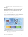

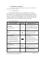
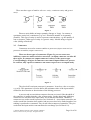
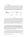
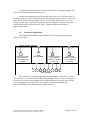
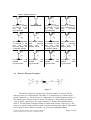
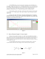
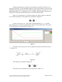
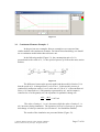
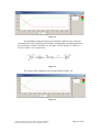
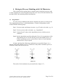
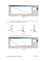
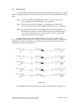

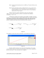
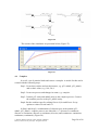
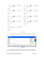
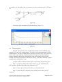
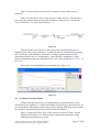
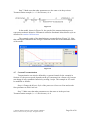
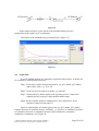
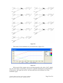
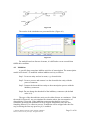
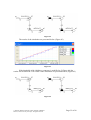
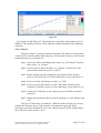
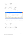
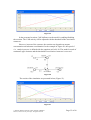
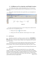
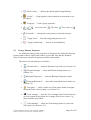

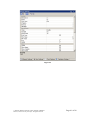

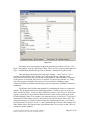

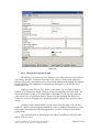

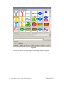
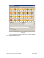
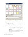
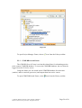
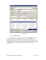
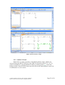
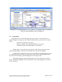
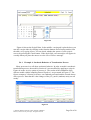
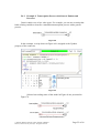
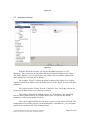

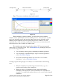

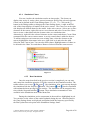
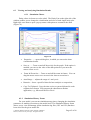
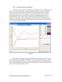
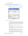

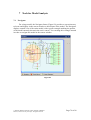
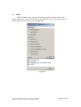
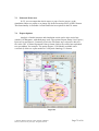
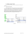


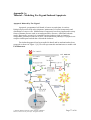

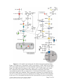
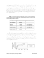
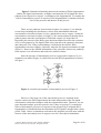


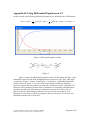
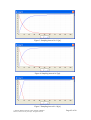
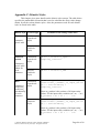


![libsbml[5pt] Developer`s Manual](http://vs1.manualzilla.com/store/data/005677524_1-a4aef53ff9933c16603010582721c07c-150x150.png)