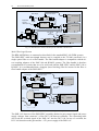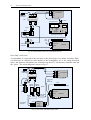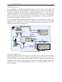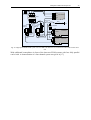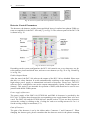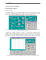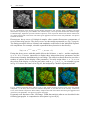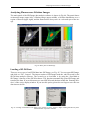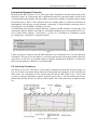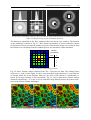
Download Modular FLIM Systems for Olympus FV1000 Laser Scanning

High Performance
Photon Counting
User Handbook
Modular FLIM
Systems for
Olympus FV1000
Laser Scanning
Microscopes
Becker & Hickl GmbH
II
Becker & Hickl GmbH
Nahmitzer Damm 30
12277 Berlin
Germany
Tel. +49 / 30 / 787 56 32
FAX +49 / 30 / 787 57 34
http://www.becker-hickl.com
email: [email protected]
1st Edition, May 2006
This handbook is subject to copyright. However, reproduction of small portions of the material in scientific papers or other non-commercial publications is considered fair use under the
copyright law. It is requested that a complete citation be included in the publication. If you
require confirmation please feel free to contact Becker & Hickl.
Contents
Contents
Introduction ...............................................................................................................................................1
Why Use FLIM....................................................................................................................................1
Requirements to a FLIM Technique ....................................................................................................4
Multi-Dimensional Time-Correlated Single Photon Counting ............................................................6
One-Photon FLIM versus Multi-Photon FLIM....................................................................................8
The FV1000 FLIM Systems......................................................................................................................11
Data Acquisition System......................................................................................................................11
One-Photon Confocal FLIM Detection Systems..................................................................................12
Picosecond Diode Laser.................................................................................................................12
Optical Interface.............................................................................................................................14
Detectors for Confocal FLIM.........................................................................................................15
Wiring Diagrams of Confocal FLIM Systems................................................................................17
Multiphoton NDD FLIM Systems .......................................................................................................22
Synchronisation with the Laser ......................................................................................................22
Optical Interface.............................................................................................................................22
Detectors for NDD FLIM ..............................................................................................................23
Wiring Diagrams of Typical NDD-FLIM Systems ........................................................................24
SPCM Software.........................................................................................................................................31
Data Acquisition ..................................................................................................................................31
Configuration of the Main Panel ....................................................................................................31
System Parameters .........................................................................................................................33
Measurement Control Parameters ..................................................................................................34
CFD, SYNC and TAC Parameters.................................................................................................36
Data Format and Page Control.......................................................................................................36
Scan Parameters .............................................................................................................................36
Access of System Parameters from the Main Panel .......................................................................37
Detector Control Parameters ..........................................................................................................38
Display of Images in the SPCM Software ...........................................................................................41
Online Display ...............................................................................................................................41
Display Parameters ........................................................................................................................41
Window Intervals...........................................................................................................................42
Saving Setup and Measurement Data ..................................................................................................44
Loading Setup and Measurement Data ................................................................................................45
Predefined Setups ................................................................................................................................46
System Setup .............................................................................................................................................49
One-Photon (Confocal) Microscopes ..................................................................................................49
Installing the Diode Laser ..............................................................................................................49
Alignment of the Laser...................................................................................................................49
Installing the Detectors ..................................................................................................................50
Multiphoton Microscopes....................................................................................................................53
Installing Non-Descanned Detectors..............................................................................................53
Installation of the SPC and DCC modules...........................................................................................53
Software .........................................................................................................................................53
Hardware........................................................................................................................................54
Getting Started: First Light ..................................................................................................................56
System Setup Parameters ...............................................................................................................56
Adjusting the CFD Parameters.......................................................................................................60
Recording Images ................................................................................................................................61
FLIM Measurements .................................................................................................................................65
Steps of a FLIM Measurement ............................................................................................................65
Details of FLIM Data Acquisition .......................................................................................................69
Synchronisation and Count Rates...................................................................................................69
Photobleaching...............................................................................................................................70
Acquisition Time of FLIM.............................................................................................................70
Image Size......................................................................................................................................72
Single-Point Fluorescence Decay and FCS Measurements .......................................................................73
Data Analysis ............................................................................................................................................75
Introduction .........................................................................................................................................75
Analysing Fluorescence Lifetime Images ............................................................................................77
III
IV
Contents
Loading of FLIM Data ...................................................................................................................77
Hot Spot and Region of Interest Selection .....................................................................................78
Instrument Response Function .......................................................................................................79
Fit Selection Parameters.................................................................................................................79
Binning in the Lifetime Analysis....................................................................................................80
Model Selection .............................................................................................................................82
Calculation of the Lifetime Image..................................................................................................85
Display of Lifetime Images..................................................................................................................85
Lifetime Parameter Histogram .......................................................................................................86
Special Commands ..............................................................................................................................86
Applications ..............................................................................................................................................89
Measurement of Local Environment Parameters .................................................................................89
Fluorescence Resonance Energy Transfer (FRET)..............................................................................89
Autofluorescence Microscopy of Tissue..............................................................................................93
References .................................................................................................................................................95
Index..........................................................................................................................................................101
Introduction
1
Introduction
This handbook describes the bh TCSPC FLIM systems for the Olympus Fluo View FV1000
laser scanning microscopes. The systems are based on bh’s proprietary multi-dimensional
TCSPC technique. The systems are modular, and a large number of system configurations are
available. The fluorescence light may be detected by one, two, or four detectors, or in 16
channels of a multi-wavelength system. Moreover, the systems may use a single TCSPC
channel, or several TCSPC channels may be used in parallel to increase the acquisition speed.
The bh FLIM systems work both for microscopes with multiphoton excitation and for microscopes with one-photon excitation. It should, however, be noted here that multiphoton excitation is covered by patents owned by Zeiss [43] and Leica [57]. The patent situation and thus
the availability of the multiphoton technique for the Fluo View FV1000 depends on the country you are living in.
This handbook should be considered a supplement to the bh TCSPC Handbook [22] and the
user manual of the FV1000. Moreover, we recommend [21] as supplementary literature.
Why Use FLIM
Since their broad introduction in the early 90s confocal and two-photon laser scanning microscopes have initiated a breakthrough in biomedical imaging [44, 67, 85, 103]. The applicability of multi-photon excitation, the optical sectioning capability and the superior contrast of
these instruments make them an ideal choice for fluorescence imaging of biological samples.
However, the fluorescence of organic molecules is not only characterised by the emission intensity and the emission spectrum, it has also a characteristic lifetime. In the simplest case, the
fluorescence lifetime can be used to distinguish between different fluorophores. Moreover, the
fluorescence lifetime is not only different for different fluorophores, it also depends on the
molecular environment of the fluorophore molecules. Any interaction between an excited
molecule and its environment in a predictable way changes the fluorescence lifetime. Since
the lifetime does not depend on the concentration of the fluorophore fluorescence lifetime
imaging is a direct approach to the mapping of cell parameters like pH, ion concentrations or
oxygen saturation, protein interaction, and other effects on the molecular scale.
The Fluorescence Decay Function
When an organic dye is excited by light of appropriate wavelength a part of the light is absorbed. A fraction of the absorbed light is converted into heat; the rest is emitted at a wavelength longer than the excitation wavelength. The effect is known as fluorescence. The fluorescence light not only has a characteristic spectrum; it is also emitted with a characteristic
time constant, the fluorescence lifetime or fluorescence decay time [75]. The fluorescence
lifetime becomes apparent if a sample is excited by light pulses shorter than a few nanoseconds, see Fig. 1.
2
Introduction
Intensity
Fluorescence
e- t /
Excitation
0
1
2
3
Time (ns) 4
Fig. 1: Decay of the fluorescence (red) after excitation with a short light pulse (blue)
In the simplest case, the fluorescence lifetime can be used as an additional parameter to separate or identify the emission of different fluorophores. The application of the lifetime as a
separation parameter is particularly useful to distinguish the autofluorescence components in
tissues. These components often have poorly defined fluorescence spectra but can be distinguished by their fluorescence lifetime [71]. FLIM has also been used to verify the laser-based
transfection of cells with GFP [100].
Fluorescence Quenching
An excited molecule can also dissipate the absorbed energy by interaction with other molecules. The effect is called fluorescence quenching. The fluorescence lifetime, τ, becomes
shorter than the normally observed fluorescence lifetime, τ0, see Fig. 2. Typical quenchers are
oxygen, halogens, and heavy metal ions, and a variety of organic molecules. The fluorescence
lifetime of most fluorophores depends more or less on the concentration of ions in the local
environment and on the oxygen concentration. For fluorescence lifetime microscopy it is important that the rate constant of fluorescence quenching depends linearly on the concentration
of the quencher. The concentration of the quencher can therefore be directly be obtained from
the decrease in the fluorescence lifetime [75].
Intensity
Unquenched
Fluorescence:
e- t / 0
Quenching:
e- t / q
0
1
2
3 Time (ns) 4
Fig. 2: Fluorescence quenching
Protonation
Many fluorescent molecules have a protonated and a deprotonated form. The equilibrium between both depends on the pH. It the protonated and deprotonated form have different lifetimes the apparent lifetime is an indicator of the pH. A typical representative of the pHsensitive dyes is 2’,7’-bis-(2-carboxyethyl)-5-(and-6)-carboxyfluorescein (BCECF) [58, 59,
75].
Complexes
Many fluorescent molecules, including endogenous fluorophores, form complexes with other
molecules, in particular proteins. The fluorescence spectra of these different conformations
Why Use FLIM
3
can be virtually identical, but the fluorescence lifetimes are often different. The exact mechanism of the lifetime changes is not always clear. In practice, it is only important that for almost all dyes the fluorescence lifetime depends more or less on the binding to proteins, DNA
or lipids [64, 74, 75, 94, 102]. The lifetime can therefore be used to probe the local environment of dye molecules on the molecular scale, independently of the concentration of the fluorescing molecules.
Extremely strong effects on the decay rates must also be expected if dye molecules are bound
to metal surfaces, especially to metallic nano-particles [51, 78].
The fluorescence behaviour of a fluorophore is also influenced by the solvent, especially the
solvent polarity [75]. Moreover, when a molecule is in the excited state the solvent molecules
around it re-arrange. Consequently, energy is transferred to the solvent, with the result that the
emission spectrum is red-shifted. Solvent (or spectral) relaxation in water happens on the time
scale of a few ps. However, the relaxation times in viscous solvents and in dye-protein constructs can be of the same order as the fluorescence lifetime. The effects can be measured by
TCSPC [89]; applications to cell imaging have not been reported yet.
Aggregation
The radiative and non-radiative decay rates depend also on possible aggregation of the dye
molecules. The electron systems of the individual molecules in aggregates are strongly coupled. Therefore the fluorescence behaviour of aggregates differs from that of the free molecules. The lifetime of aggregates can be longer than that of single molecules; on the other
hand, the fluorescence may be almost entirely quenched. Aggregation is influenced by the
local environment; the associated lifetime changes can be used as a probe function. Aggregation has also been used to observe the internalisation of dyes into cells [63]. However, in most
applications aggregation is to be avoided by keeping the dye concentration at a reasonable
level.
FRET
A particularly efficient energy transfer process between an excited and a non-excited molecule
is fluorescence resonance energy transfer, or FRET. The effect was found by Theodor Förster
in 1946 [50]. The effect is also called Förster resonance energy transfer or simply resonance
energy transfer (RET). Fluorescence resonance energy transfer is an interaction of two molecules in which the emission band of one molecule overlaps the absorption band of the other.
In this case the energy from the first dye, the donor, transfers immediately into the second one,
the acceptor. The energy transfer itself does not involve any light emission and absorption.
FRET can result in an extremely efficient quenching of the donor fluorescence and consequently in a considerable decrease of the donor lifetime; see Fig. 3.
Intensity
Intensity
Laser
Donor
Absorption
Donor
Emission
Acceptor
Absorption
Acceptor
Emission
e -t/
Excitation
D
D
A
A
Emission
e -t/
0
FRET
quenched
donor
Wavelength
unquenched donor
Time
Fig. 3: Fluorescence Resonance Energy Transfer (FRET)
The energy transfer rate from the donor to the acceptor decreases with the sixth power of the
distance. Therefore it is noticeable only at distances shorter than 10 nm [75]. FRET is used as
a tool to investigate protein-protein interaction. Different proteins are labelled with the donor
4
Introduction
and the acceptor, and FRET is used as an indicator of the binding state of these proteins. Distances on the nm scale can be determined by measuring the FRET efficiency quantitatively.
Requirements to a FLIM Technique
Time Resolution
It is sometimes believed that FLIM in cells does not require a particularly high time resolution. It is certainly correct that the fluorescence lifetimes of most fluorophores used in cell
imaging are on the order of a few ns. However, the lifetime of autofluorescence components
and of the quenched donor fraction in FRET experiments can be as short as 100 ps. Lifetimes
of dye aggregates in cells have been found as short as 50 ps [63]. The lifetime of fluorophores
bound to metallic nano-particles [51, 78] can be 100 ps and shorter. A good FLIM technique
should therefore by able to record lifetimes down to less than 100 ps. Moreover, it should be
able to resolve the components of complex decay profiles, see below.
Decay Profiles of Biological Samples
The fluorophore populations in biological specimens are normally not homogeneous. Several
fluorophores may be present in the same pixel, or one fluorophore may exist in different binding or protonation states. The fluorescence decay functions are therefore usually multiexponential. A few typical decay profiles are shown in Fig. 4.
Fig. 4: Decay profiles of biological samples, total length of time axis 10 ns, logarithmic intensity scale. Left to
right: CFP-YFP FRET in HEK cell at emission wavelength of CFP, autofluorescence of the stratum corneum of
human skin, plant tissue sample
The curves show the fluorescence intensity versus the time in the fluorescence decay. The
total length of the time axis is 10 ns; the intensity scale is logarithmic. All curves were measured by TCSPC FLIM. The blue dots are the photon numbers in the subsequent time channels
of a selected image region; the red curve is a fit by a double-exponential or triple-exponential
model. Even without data analysis, it is clearly visible that the decay profiles are not single
exponentials.
In the case of CFP-YFP FRET the decay profile can be fitted well by a double-exponential
model. The fit delivers a lifetime of 590 ps for the interacting donor component, a lifetime of
2.4 ns for the non-interacting donor component, and the respective amplitudes of 51 % and
49 %.
The fluorescence decay of skin autofluorescence is fit by two components of 208 ps and
2.1 ns, with amplitudes of 77 % and 23 %. For the plant tissue even a double-exponential fit is
not satisfactory. A triple-exponential fit delivers 150 ps, 313 ps, and 1716 ps, with amplitudes
of 53 %, 39 % and 8.8 %, respectively.
There are certainly cases when fitting multi-exponential decay profiles by a single-exponential
decay is feasible. These may be pH imaging, oxygen quenching experiments, or ion concentra-
Requirements to a FLIM Technique
5
tion measurements. Even in FRET experiments a single-exponential fit is acceptable if only
the locations of protein interaction in a cell, not the quantitative values are required. In most
cases, however, describing the fluorescence of the sample by a single ‘Fluorescence Lifetime’
means discarding useful information or even leads to wrong conclusions.
Efficiency
Under ideal conditions, the lifetime of a single-exponential decay can be obtained from the
recorded data with the same accuracy as the intensity [4, 52, 65]. In both cases the standard
deviation is N , with N being the number of photons in the pixel considered. One might
therefore conclude that FLIM does not set special requirements to the photon economy. Unfortunately this is not so. An intensity image with a standard deviation of 10% may look pleasing and show the spatial structure of a sample very well. However, lifetime changes investigated by FLIM may be on the order of a few %. Thus, a standard deviation on the order of 1 %
is required. Thus, except for a few relatively trivial cases, FLIM experiments need to record a
large number of photons.
An even larger number of photons is required for resolving the components multi-exponential
decay functions. Köllner and Wolfrum [65] calculate a number of 400.000 photons for resolving two decay components of 2 ns and 4 ns, with amplitudes of 10% and 90%, respectively.
Of course, resolving such decay functions in FLIM images is almost impossible. Fortunately,
in practice the lifetimes are wider apart, and the amplitude of the fast component is larger.
Such decay profiles can be resolved by analysing some 1000 photons per pixel, see Fig. 4.
Nevertheless, a large number of photons must be recorded.
Recording many photons means either a high excitation intensity or a long acquisition time.
Therefore photobleaching [45, 83] and photodamage [60, 66, 69] are important issues in precision FLIM experiments. Both effects are more troublesome for FLIM than for intensity imaging because they are likely to change the lifetimes [17]. Photobleaching and photodamage
are clearly nonlinear for two-photon excitation. A nonlinear component seems to be present
also for high intensities of one-photon excitation [28]. A good FLIM technique must therefore
not only make best use of the detected photons, it must also be able to work reliably at low
intensity.
Multi-Wavelength Detection
In some cases FLIM images are taken in several emission wavelength intervals or under different angle of polarisation. It is important that both recordings be performed simultaneously.
This not only reduces the sample exposure and the associated photobleaching, it also avoids
that the photobleaching of the first recording changes the results of the second one. Only if
both recordings are done simultaneously the results are comparable.
Compatibility with the Scanning Microscope
Laser scanning microscopes with standard scanners scan the sample at pixel dwell times down
to about 1 µs, systems with resonance scanners even faster. Photon rates obtained from typical
samples are usually an order of magnitude smaller. It is thus impossible to obtain enough photons for lifetime analysis within the time the beam is on one pixel. Consequently, the FLIM
system must be able to acquire the photons from a large number of frames scanned at a pixel
rate higher than the photon detection rate.
Another important issue is lateral resolution and depth resolution. Mixing the fluorescence
lifetimes of different sample planes or different locations of the sample must be strictly
avoided. Thus, the FLIM technique must make full use of the depth resolution of confocal and
two-photon laser scanning microscopes [21].
6
Introduction
Multi-Dimensional Time-Correlated Single Photon Counting
Time-correlated single photon counting (TCSPC) is an amazingly sensitive technique for recording low-level light signals with picosecond resolution and extremely high precision.
TCSPC is based on the detection of single photons of a periodic light signal, the measurement
of the detection times, and the reconstruction of the waveform from the individual time measurements. The technique in its classic form is successfully used since the early 70s [82, 104].
Due to the low intensity and low repetition rate of the light sources and the limited speed of
the electronics of the 70s and 80s the acquisition times of classic TCSPC applications were
extremely long. More important, classic TCSPC was intrinsically one-dimensional, i.e. limited
to the recording of the waveform of a periodic light signal. For many years TCSPC was therefore used primarily to record fluorescence decay curves of organic dyes in solution. A few
attempts were made to use TCSPC in combination with scanning microscopes [37]. However,
the classic TCSPC technique was limited not only to relatively low count rates but also to
slow scanning [36].
The situation changed with the introduction of the multi-dimensional TCSPC technique of
Becker & Hickl. The new technique not only increased the recording speed by two orders of
magnitude [10, 13], it also added additional dimensions to the recording process. The photon
distribution is recorded not only versus the time in the fluorescence decay but also versus the
coordinates of a scanning area [16], the wavelength [14], or the time from the start of the experiment [10, 18]. The technique is extremely flexible, and the configuration of the hardware
can be changed by a simple software command. Multi-dimensional TCSPC is described in
detail in [21, 22].
TCSPC makes use of the special properties of high-repetition rate optical signals detected by a
high-gain detector. Understanding these signals is the key to the understanding of TCSPC.
The situation is illustrated in Fig. 5.
Excitation pulse sequence, repetition rate 80 MHz
a
100ns
Fluorescence signal (expected)
b
Detector signal, oscillocope trace
c
Fig. 5: Detector signal for fluorescence detection at a pulse repetition rate of 80 MHz
Fluorescence of a sample is excited by a laser of 80 MHz pulse repetition rate (a). The expected fluorescence waveform is (b). However, the detector signal measured by an oscilloscope has no similarity with the expected fluorescence waveform. Instead, it consists of a few
pulses randomly spread over the time axis (c). The pulses represent the detection of single
photons of the fluorescence signal.
The photon detection rate (c) is about 107 s-1. This is on the order of the maximum possible
detection rate of most detectors, and far above the count rates available from a living specimen in a scanning microscope. Thus, the fluorescence waveform (c) has to be considered a
probability distribution of the photons, not anything like a directly observable signal waveform. Moreover, Fig. 5 shows clearly that the detection of a photon in a particular signal pe-
Multi-Dimensional Time-Correlated Single Photon Counting
7
riod is a relatively unlikely event. The detection of several photons in one signal period is
even less likely.
The idea behind TCSPC is that only one photon per signal period needs to be considered. If
only one photon needs to be detected per signal period the build-up of a photon distribution
over the time in the signal period, and, in case of multi-dimensional TCSPC, over additional
parameters is a straightforward task. Of course, the neglecting of a possible second photon and
the resulting ‘pile-up effect’ are subject of never-ending discussion. It can, however, be
shown, that the effect on the recorded lifetime under practical conditions is negligible [21].
The architecture of a multi-dimensional TCSPC device operated in the FLIM mode is shown
in Fig. 6.
PMTs
Channel
Channel register
n
Channel / Wavelength
Router
Time
Measurement
Timing
Start
CFD
TAC
Stop
from Laser
t
ADC
CFD
Frame Sync
Counter Y
Line Sync
Scanning
Interface
Pixel Clock
Counter X
from
Time within decay curve
y
x
Histogram
Memory
Detector
channel 1
Histogram
Memory
Detector
channel 2
Histogram
Memory
Detector
channel 3
Histogram
Memory
Detector
channel 4
Location within scanning area
Microscope
Fig. 6: Multidimensional TCSPC in the FLIM mode
At the input of the detection system are a number of photomultipliers (PMTs), detecting the
fluorescence light from the excited spot of the sample in different wavelength intervals.
In the subsequent ‘router’ the single-photon pulses of the PMTs are combined into a common
timing pulse line. The combination is possible because the photon count rate is considerably
smaller than the repetition rate of the laser [21] (see Fig. 5). The timing pulse is sent through
the time-measurement block of the TCSPC device. This block determines the time of the photon in the laser pulse period.
Along with the timing pulse, the router delivers the number, n, of the PMT in which a photon
was detected. The detector number is stored in the ‘channel register’ of the TCSPC device.
The detector number is used later to store the photons of the individual detectors in different
memory blocks. The routing technique can be used with several individual PMTs and with
multi-anode PMTs [22].
The scanning interface of the TCSPC module receives the scan clock signals (pixel, line, and
frame clock) from the scanning unit of the microscope. For each photon, the TCSPC module
determines the location within the scanning area, x and y. The photon times, t, the detector
channel number, n, and the spatial coordinates, x and y, are used to address a memory in
which the detection events are accumulated. Thus, in the memory the distribution of the photon density over x, y, t, and n builds up. The result can be interpreted as a number of data sets
for the individual detectors, each containing a large number of images for consecutive times in
8
Introduction
the fluorescence decay. The individual data sets can also be considered images with a fluorescence decay curve stored in each pixel.
The data acquisition runs at any scanning speed of the microscope. As many frame scans as
necessary to obtain an appropriate signal-to-noise ratio can be accumulated. At the typical
count rates obtained from living specimens the pixel rate is higher than the photon count rate.
This makes the recording process more or less random; a photon is just stored in a memory
location according to its time in the fluorescence decay, its detector channel number, and the
location of the laser spot in the sample in the moment of detection.
It should be noted that multi-dimensional TCSPC does not use any time gating, wavelength
scanning, or detector multiplexing. For count rates up to several MHz virtually all detected
photons contribute to the result. Consequently, a near-ideal signal-to-noise ratio for a given
fluorescence intensity and acquisition time is obtained.
The time resolution is determined mainly by the transit time spread of the detectors. With
multichannel PMTs the width of the instrument response function (IRF) is about 30 ps (full
width at half maximum, fwhm); with the PMC-100 detectors an IRF about 150 ps (fwhm) is
achieved.
The fluorescence decay curves in the individual pixels of the image are resolved into a large
number - typically 64 to 1024 - time channels. The large number of time channels in combination with the near-ideal counting efficiency results in a near-ideal standard deviation of the
measured fluorescence lifetime over a wide range of lifetimes [65]. Moreover, standard multiexponential lifetime analysis techniques can be used to resolve complex decay profiles into
their lifetime components and intensity coefficients.
It should also be mentioned that multi-dimensional TCSPC FLIM does not require any calibration by a lifetime standard. Lifetime standards are difficult to use because the effective
fluorescence lifetime depends on the pH and the possible presence of fluorescence quenchers,
see ‘Fluorescence Quenching’, page 2. For the bh FLIM systems the time scale of the TCSPC
module is factory calibrated and the fluorescence decay is recorded into a large number of
time channels; thus data analysis automatically delivers absolute lifetimes.
By a simple change of the operation mode (see ‘System Parameters’, page 33) the TCSPC
modules can be configured for a number of different signal recording procedures.
In particular, the ‘FIFO’ or ‘Time-Tag’ can be used to simultaneously obtain fluorescence
correlation (FCS) [27, 49, 77, 91], photon counting histograms (PCHs) [39, 81] and fluorescence decay curves in selected spots of a sample [19, 21, 23]. The technique can even be used
to identify the photon bursts of individual molecules and run a lifetime and anisotropy analysis with the bursts. The technique is termed ‘Burst integrated fluorescence lifetime analysis, or
BIFL [21, 47, 89].
The sequential recording modes can be used to acquire fast triggered sequences of decay
curves or even small images at high speed. Typical applications are electro-physiology experiments or chlorophyll transients [6, 21, 22]. It should, however, be noted that most of these
techniques are not finally explored or even tested in conjunction with commercially available
laser scanning microscopes.
One-Photon FLIM versus Multi-Photon FLIM
As described above, FLIM requires a pulsed excitation source of both high repetition rate and
picosecond pulse duration. This may be a picosecond diode laser, a frequency-doubled
Ti:Sapphire laser, or the Ti:Sapphire laser of a multiphoton microscope. In terms of FLIM
signal recording there is no difference between these systems. There is, however, a difference
One-Photon FLIM versus Multi-Photon FLIM
9
in the way the sample is excited and the fluorescence light is detected. This results in a number of optical differences which are discussed below.
It should also be noted here that multiphoton excitation is covered by patents owned by Zeiss
[43] and Leica [57]. The patent situation and thus the availability of the multiphoton technique
for the FV1000 depends on the country you are living in.
The general optical principle of a laser scanning microscope [44, 79, 85] is shown in Fig. 7.
One-photon excitation is shown left, two-photon excitation right.
ps Diode
Laser
Pinhole
Pinhole
Dichroic
Mirror
Detector
Confocal
Scanner
Ti:Sa
Laser
Dichroic
Mirror
Detector
Confocal
Scanner
Detector
Dichroic
Mirror
NDD
Excited
Objective
Lens
Sample
One-Photon Excitation
Excited
Objective
Lens
Sample
Two-Photon Excitation
Fig. 7: One-photon FLIM (left) and multi-photon FLIM (right)
One-Photon Excitation With Confocal Detection
The laser is fed into the optical path via a dichroic mirror and focused into the sample by the
microscope objective lens. Scanning is achieved by deflecting the beam by two galvanometerdriven mirrors. The excitation light excites fluorescence within a double cone throughout the
whole depth of the sample. The fluorescence light from the sample goes back through the objective lens, and through the scanner. After travelling back though the scanner the beam of
fluorescence light is stationary or ‘descanned’. The light is focused into a confocal pinhole in
an image plane conjugate with the image plane in the sample. Light from outside the focal
plane is not focused into the pinhole and therefore substantially suppressed [44, 85, 103]. Outof-focus suppression is the basis of the superior image quality and the optical sectioning capability of scanning systems. For FLIM out-of-focus suppression is even more important. Any
mixing of the (possibly different) fluorescence lifetimes of different focal planes adds additional lifetime components to the apparent decay functions. However, the difficulties of unmixing lifetime components increase dramatically with the number of components. Out-offocus suppression is therefore mandatory to obtain good FLIM results.
Two-Photon Excitation With Descanned Detection
With a fs Ti:Sa laser the sample can be excited by two-photon absorption [42, 53]. The efficiency of two-photon excitation increases with the square of the excitation power density.
Noticeable excitation is therefore obtained only in the focus. Thus, two-photon excitation is a
second way to obtain depth resolution and suppression of out-of-focus fluorescence, see Fig.
7, right. Different from one-photon excitation and confocal detection, which avoids out-of
focus detection, two-photon excitation avoids out-of-focus excitation. Therefore, detection
through a confocal pinhole is not required to obtain a good image quality. Nevertheless, feeding the fluorescence light back through the scanner and the pinhole often has benefits. The
10
Introduction
accuracy of FLIM can be seriously impaired by detection of background light and by optical
reflections in the beam path. A pinhole, even if wide enough to transmit virtually all fluorescence light, yields substantial suppression of daylight and of optical reflections.
Two-Photon Excitation With Direct Detection
Since the scattering and the absorption coefficients at the wavelength of the two-photon excitation are small the laser beam penetrates through relatively thick tissue. Two-photon excitation can therefore be used to excite fluorescence in tissue layers as deep as 1 mm [42, 44, 67,
68, 85, 86, 98, 99]. The problem of deep-tissue imaging is, however, that the fluorescence
photons are strongly scattered on their way out of the sample and emerge from a relatively
large area of the sample surface. Moreover, the surface is not in the focus of the objective
lens. No matter which optical system is used, it is impossible to focus this light into a pinhole.
The solution to deep-tissue imaging is ‘direct’ or ‘non-descanned’ detection. The fluorescence
light is diverted by a dichroic mirror directly behind the microscope lens and transferred into a
detector, see Fig. 7, right. Thus, photons leaving the sample from a large area are collected
and fed into the detector.
Unfortunately the large detection area of a direct detection system has also a drawback: It increases the detection efficiency for scattered photons and for photons of background light
similarly. Any direct detection system with TCSPC has therefore to be operated in absolute
darkness.
The FV1000 FLIM Systems
11
The FV1000 FLIM Systems
The bh FLIM systems are modular [22]. Consequently, a large number of system configurations are available. The excitation light source can be a picosecond diode laser attached to a
confocal microscope or the Ti:Sapphire laser of a multiphoton microscope. The detection light
path may the a fibre output from the scan head of the FV1000, a direct output form the
FV1000 scan head, or a non-descanned (direct) output of an FV1000 that is operated as a
multiphoton microscope. The fluorescence light may be detected by one or two detectors [15],
or in 16 channels of a multi-wavelength system [6, 14, 21, 29, 33, 95]. Depending on the particular application different detectors may be used [22]. Moreover, the systems may use a single TCSPC channel, or several TCSPC channels may be used in parallel to increase the acquisition speed [17, 21, 22].
Data Acquisition System
Most confocal and NDD FLIM systems use the bh SPC-830 module for data acquisition. In
systems that use a single bh DCC-100 detector or the bh MW-FLIM setup the detector signal
is connected directly to the stop input of the SPC-830 module. The R3809U and H7422P-40
detectors [55, 56] are connected via preamplifiers. Dual-detector systems require an HRT-41
router [5, 22] to connect both detectors to a single SPC-830 module. Alternatively, two
SPC-140 or SPC-150 modules can be used with the detectors connected directly to the
TCSPC modules. The components of the data acquisition system are shown in Fig. 8.
Fig. 8: Components of the FLIM data acquisition systems. Left to right: SPC-830 TCSPC FLIM module, preamplifier for R3809U and H7422P-40 detectors, HRT-41 router for simultaneous operation of several detectors at
one SPC-830 module
The detectors of the bh FLIM systems are controlled via a DCC-100 detector controller card.
The card supplies the power to the detectors, controls the shutters of NDD-FLIM systems,
provides software control of the detector gain and shuts down the detectors in case of overload. The DCC-100 card is shown in Fig. 9.
Fig. 9: DCC-100 detector controller
The SPC-830 module and the DCC-100 detector/shutter controller may be operated in a standard PC, or the ‘Simple Tau’ lap-top based system [22] may be used. The ‘Simple Tau’ has
the SPC-830 and the DCC-100 module readily installed in an extension box of the lap-top
computer. This makes the data acquisition system compact and portable, see Fig. 10.
12
The FV1000 FLIM Systems
Fig. 10: ‘Simple Tau’ compact data acquisition system.
The Simple Tau can be used for all configurations that require no more than one TCSPC
module and one DCC-100 detector controller card and.
To increase the acquisition speed of TCSPC FLIM systems several detector and TCSPC channels can be operated in parallel [17]. Systems with up to four channels are supported by the
data acquisition software. Any set of similar TCSPC-FLIM modules (SPC-830, SPC-140 or
SPC-150) can be used. However, size and cost considerations normally lead to systems containing several SPC-140 or SPC-150 cards, see Fig. 11.
Fig. 11: Package of four parallel SPC-140 channels for high speed FLIM applications
Two- and four-channel TCSPC systems require additional beamsplitters at the optical outputs
of the FV1000 microscope. Four-channel TCSPC systems have a saturated count rate of
40⋅106 photons per second and can be reasonably operated at a (recorded) total count rates up
to of 20⋅106 s-1. Thus, single-exponential lifetime images can be obtained within acquisition
times as shorter than a second [17, 21]. It should be noted, however, that most samples do not
deliver count rates this high without substantial photobleaching. Therefore, please make sure
that the photostability of the samples you are going to investigate is high enough to justify the
cost of a two- or four-channel TCSPC system.
One-Photon Confocal FLIM Detection Systems
Picosecond Diode Laser
Fluorescence lifetime imaging requires a pulsed excitation source. This is no problem in
multi-photon microscope. The titanium-sapphire laser meets the requirements of TCSPC
FLIM almost ideally. Standard Fluo View FV1000 microscopes, however, use continuous
lasers. To upgrade these systems for FLIM a pulsed excitation source must be added. The bh
FLIM systems use a BDL-405SMC picosecond diode laser for excitation. This laser has a
One-Photon Confocal FLIM Detection Systems
13
wavelength of 405 nm1. The laser can be operated both in CW mode and picosecond pulsed
mode. In the pulsed mode, the repetition rate can be switched between 20 MHz, 50 MHz, and
80 MHz. The pulse width is about 60 ps. Higher repetition rate gives higher average power.
However, the fluorescence may not completely decay between the pulses. Incomplete decay
can, in principle, be taken into account in the data analysis, but results in less than optimal
standard deviation of the lifetime. For most of the fluorophores, including the GFPs, 50 MHz
repetition rate is the best compromise.
The BDL-405SMC laser [9] is shown in Fig. 12. The laser head (shown right) contains the
complete driving electronics. Confocal laser scanning microscopes use single-mode fibres to
transfer the light of the excitation lasers into the scan head. It is therefore essential to couple
the light of the laser diode efficiently into the fibre. For laser diodes this is difficult because
the beam generated by a laser diode has a high divergence, non-circular shape, and substantial
astigmatism. The BDL-405SMC laser therefore has a beam profile corrector that corrects both
for beam shape and astigmatism. As a result, more than 60% of the laser power are coupled
into the single-mode fibre2. The power available from the single-mode fibre of a 405 nm laser
is about 1 mW and 30 mW for pulsed and CW operation, respectively.
The optical output of the laser is coupled to the 405 nm input fibre of the FV1000. The input
fibres of the FV1000 use the connector system of Point Source Ltd., UK. The BDL-405SMC
lasers for the FV1000 FLIM systems are therefore delivered with a Point-Source-compatible
fibre adapter, see Fig. 12, right. For alignment of the fibre coupler, please see Fig. 50, page 50.
The BDL-405SMC is operated from a simple wall-mounted 12 V power supply (Fig. 12, left).
A control box (Fig. 12, middle) is inserted in the power and control cable to the laser. This
box contains the frequency selection switch, and the mandatory safety key switch and emission indicator LEDs.
A timing synchronisation signal is provided at an SMA connector at the back of the laser. The
polarity of the pulses is positive; therefore an A-PPI-pulse inverter has to be used in the
SYNC line of the SPC-830 module.
Fig. 12: BDL-405SMC picosecond diode laser. Left: Power supply. Middle: Control box. Right: Laser with beam
profile corrector and coupler for single-mode fibre
The bh BDL lasers have an input for electronic control of the optical output power. The connector is located at the back of the control box. In the bh FLIM systems, the power control
input is driven by a signal from the bh DCC-100 detector controller.
Moreover, all bh BDL lasers have an input for fast on/off control. The on/off input was implemented for beam blanking during the line and frame flyback, and for FRAP applications.
1
Versions with 375 nm, 440 nm, and 473 nm wavelength are available. However, the available laser input at the
FV1000 is not necessarily compatible with these wavelengths, due to the internal dichroic mirrors of the scan
head.
2
The beam corrector is a development of LASOS GmbH, Jena, Germany
14
The FV1000 FLIM Systems
The standard FV1000 FLIM systems do not use the beam-blanking capability of the
BDL-405SMC laser. Please contact bh if you need beam blanking.
Optical Interface
One-photon excitation requires confocal detection to achieve suppression of out-of focus light,
see Fig. 7, page 9.
The scan mirrors, the pinhole, and the dichroic mirror that separates the fluorescence light
from the excitation light are contained in the Olympus FV1000 scan head. The scan head contains several photomultipliers detecting the fluorescence signal in selectable wavelength intervals. Unfortunately, these detectors and the associated preamplifiers are not fast enough for
reasonable FLIM data acquisition. Upgrading the FV1000 scanning microscope therefore requires one or several fast detectors to be attached to an optical output from the FV1000 scanner. The designers of the Olympus Fluo View FV1000 have provided for such an output in
form of a fibre port. Although the fibre port can easily be used to transfer the light to a FLIM
detector it is not the favoured FLIM solution for two reasons:
The first one is that the multi-mode fibre used introduces pulse broadening. The effect is noticeable only for ultra-fast detectors, such as the R3809U, but nevertheless unwelcome. The
second reason for not using fibre coupling is efficiency. Coupling into the fibre inevitably
causes loss in intensity - in case of the FV1000 fibre port up to 60 %.
Except for the id-100 SPAD detector, which requires a fibre connection, the bh FLIM systems
therefore use direct optical coupling The fibre adapter is removed (or not installed altogether),
and an a direct coupling optics attached instead. The FLIM adapter is shown in Fig. 13. The
FLIM beam pass contains a long-pass or bandpass filter and, in case of the R3809U detector,
an electronically controlled shutter. Details are shown in Fig. 51 and Fig. 52, page 51.
Fig. 13: Olympus Fluo View FV1000 scan head with bh FLIM adapter and FLIM detector attached. The detector
is an R3809U MCP PMT.
The shutter is used to protect the R3809U MCP PMT against high light intensities from the
microscope lamp. The other detectors are sufficiently protected by the overload shutdown
function of the DCC-100 detector controller. They are therefore operated without a shutter.
For dual-detector operation bh provide suitable shutter/beamsplitter assemblies. Both dichroic
and polarising beamsplitters are available. An example is shown in Fig. 14.
One-Photon Confocal FLIM Detection Systems
15
Fig. 14: Dual-detector assembly with two R3809U MCP PMTs. Both dichroic and polarising beamsplitters are
available.
Detectors for Confocal FLIM
Detectors for the FV1000 confocal FLIM systems are shown in Fig. 15. All PMT-based detectors are controlled via the DCC-100 detector controller card, see Fig. 22.
Fig. 15: Detectors for confocal FLIM systems. Upper row, left to right: R3809U MCP PMT, PMC-100, H7422P40, id-100-50. Bottom: PML-SPEC multi-wavelength setup.
R3809U
The R3809U detector [55] is the detector for ultimate time resolution. Its instrument response
function (IRF) has a width of 30 ps (FWHM) [22]. However, if the R3809U is used in onephoton excitation systems the pulse width of the diode laser limits the resolution. The effective IRF is thus about 60 ps. In other words, the gain in time resolution over a PMC-100 detector is only a factor of 2.5. Nevertheless, the R3809U is highly recommendable for FRET
experiments. Quantitative FRET requires the decay components of the interacting and noninteracting donor fractions to be separated. This requires a detector response that is not only
short but also free of tails or bumps after the main peak. FRET measurements benefit therefore considerably from the clean response of the R3809U.
Other applications of the R3809U are autofluorescence measurements. Autofluorescence of
cells and tissue contains several fluorescence components with lifetimes as short as 100 ps.
The fast response of the R3809U makes it easier to resolve the complex decay profiles.
16
The FV1000 FLIM Systems
The maximum continuous count rate of the R3809U is about 1⋅106 photons per second3. Although this is enough for the majority of applications it should be noted that the R3809U is
not a solution to fast-acquisition FLIM. To achieve maximum safety against overload damage
the R3809U is connected to the scan head via a shutter.
PMC-100
The PMC-100 PMT module is the standard detector for all bh FLIM systems. It delivers an
IFR of 150 ps FWHM [22]. Lifetimes down to about 200 ps are easily resolved. The PMC100 features excellent timing stability at high count rates. It can therefore be used up to the
highest count rates applicable with the bh TCSPC boards, without noticeable degradation in
the IRF [22]. Typical applications are pH imaging, oxygen imaging, and ion concentration
measurements via fluorescence quenching. The PMC-100 works well also for singleexponential FRET measurements i.e. experiments that do not require separating of the interacting and non-interaction donor fraction. Separating the different donor fractions of FRET is
generally possible. However, the longer IRF makes the data analysis more difficult and less
accurate than for the R3809U. Autofluorescence imaging is possible as well, though with
some compromise in resolution for the shortest lifetime components. All in all, the PMC-100
is the most versatile detector for one-photon FLIM systems.
H7422P-40
The H7422P-40 detector [56] has an exceptionally high quantum efficiency. It is recommended for applications that require ultimate sensitivity. In the wavelength range of 500 to
600 nm a sensitivity improvement of a factor of 2 to 3 over the R3809U and the PMC-100 is
obtained. The IRF width of the H7422P-40 is 250 to 350 ps [22]. The large IRF width makes
the H7422P-40 less useful for FRET and autofluorescence imaging. The H7422P-40 is currently the best compromise for systems that are to be used both for FLIM and FCS [19, 23,
49].
id-100-50-SMC Single-Photon Avalanche Photodiode
The id-100-50 SMC is a single-photon avalanche photodiode. The instrument response width
of the id-100-50 itself is about 45 ps. However, in one-photon systems the effective IRF is a
convolution of the laser pulse shape and the detector IRF. Thus, the typical IRF width of the
complete system is on the order of 80 ps. The id-100-50 is overload-proof; an overload shutdown function is not required. Because the id-100-50 SMC has a fibre input, it is connected to
the standard fibre output of the FV1000 scan head.
Due to its fast response the id-100-50 is an alternative to the R3809U MCP PMT. Some care
is, however, recommended if the id-10-50 is used at wavelengths longer than 500 nm. All single-photon APDs show a ‘diffusion tail’ in their response [21, 22]. The relative amplitude of
the tail increases with increasing wavelength. The diffusion tail can therefore easily be mistaken for a fluorescence component. Especially in double-exponential FRET experiments the
diffusion tail makes it difficult to accurately resolve the decay components of the interacting
and non-interacting donor fractions.
3
The R3809U can be used at count rates up to 3 MHz [21, 22]. However, the output current at this count rate is
beyond the permissible maximum specified by Hamamatsu. In FLIM applications high count rates normally occur only in a few pixels of the image. Immediate damage under these conditions appears therefore unlikely; nevertheless life cannot be guaranteed.
One-Photon Confocal FLIM Detection Systems
17
MW-FLIM
The MW FLIM detection system [6] detects the fluorescence simultaneously in 16 wavelength
channels. A polychromator splits the light spectrally and projects the spectrum on the photocathode of a PML-16 detector. This detector contains a 16 channel PMT and the associated
routing electronics [6]. Thus, 16 lifetime images are recorded in a single SPC-830 TCSPC
module. For confocal detection the MW FLIM system can be coupled both to the fibre output
of the FV1000 scanner or to the bh FLIM adapter. In the second case the light is transferred
into the polychromator via a fibre bundle. Despite of the non-ideal filling factor of the bundle
the efficiency for the fibre bundle is slightly higher than for the single fibre. Typical applications of the MW-FLIM detector are FRET experiments [33] and autofluorescence imaging
[22].
Wiring Diagrams of Confocal FLIM Systems
Connecting diagrams of some typical one-photon confocal FLIM systems are shown in Fig. 16
through Fig. 20.
PMC-100 System
The wiring diagram of a confocal FLIM system with a single PMC-100 detector is shown in
Fig. 16. A BDL-405-SMC or BDL-473-SMC diode laser is used for excitation. The optical
output of the laser is coupled to an input fibre of the FV1000 scan head. The power of the laser is controlled via connector 1 of the DCC-100 detector controller.
The fluorescence light is fed into a PMC-100 detector via a direct output from the confocal
scan head of the FV1000. To separate the fluorescence light from scattered excitation light it
is important that a suitable longpass or bandpass filter be inserted in front of the PMC-100
input. For optical configuration please see Fig. 51, page 51.
Laser Power Control
Power Supply
80 50
cont
20
Con 1
DCC-100 Board
Con 2
Power
& Control
Con 3
BDL-405 SM
Single-Mode
Fibre into
Microscope
A-PPI
Laser Sync Output
PMC100
Scan Clocks
from
Microscope
SYNC
Scan Clocks
FLIM adapter
Power Supply
& Control
Routing
SPC Board
CFD
Fig. 16: One-photon confocal FLIM system with PMC-100
The +12V power supply, the cooling current, and the gain control signal for the PMC-100 are
provided at connector 3 of the DCC-100. The cooling circuit of the DCC-100 must be configured for ‘one detector’, see DCC-100 manual [7]. The connecting cable has also a line for the
overload signal of the PMC-100. In case of overload the DCC-100 shuts down the gain control signal and the +12V power supply of the PMC-100.
The detector pulses are fed into the CFD input of an SPC-830 TCSPC FLIM module. The
timing reference signal (SYNC) signal of the TCSPC module is obtained directly from the
18
The FV1000 FLIM Systems
BDL-405SMC laser. The BDL-405SMC delivers positive synchronisation pulses; therefore an
A-PPI pulse inverter is inserted in the SYNC line. The scan clock signals of the microscope
controller are connected to the upper sub-D connector of the SPC-830 or SPC-730 module.
id-100-50 System
Fig. 17 shows a FLIM system that uses an id-100-50 single-photon avalanche photodiode as a
detector. The excitation part is the same as for the PMC-100 system described above.
The light signal from the scan head is fed through a filter adapter into the optical input of the
id-100-50 module. The id-100-50 gets its power supply voltage from the DCC-100 detector
controller. The single-photon pulses of the id-100-50 are inverted by an A-PPI pulse inverter
and fed into the ‘CFD’ input of the SPC-830 TCSPC board.
Laser Power Control
Power Supply
80 50
cont
20
Con 1
DCC-100 Board
Con 2
Power
& Control
Con 3
BDL-405 SM
Single-Mode
Fibre into
Microscope
A-PPI
Laser Sync Output
Scan Clocks
from
Microscope
Fibre
from
Scan
Head
Filter
SYNC
id-100-50
Scan Clocks
A-PPI
Fibre
Routing
SPC Board
CFD
Fig. 17: One-photon confocal FLIM system with id-100-50 detector
The id-100-50 detector is overload-proof up to light intensities far above the daylight level.
An overload shutdown is therefore not necessary.
R3809U Systems
The connecting diagram of an R3809U FLIM system is shown in Fig. 18. A BDL-405SMC or
BDL-473-SMC diode laser is used for excitation. The optical output of the laser is coupled to
an input fibre of the FV1000 scan head. The power of the laser is controlled via connector 1 of
the DCC-100 detector controller.
To provide maximum safety against detector damage all R3909 systems use electromechanical shutters in the beam path. The shutter is controlled via connector 2 of the
DCC-100 card. The operating voltage of the R3809U detectors is provided by an
FuG HCN 14-3500-A high-voltage power supply. The high voltage is controlled by a signal
from connector 3 of the DCC card.
One-Photon Confocal FLIM Detection Systems
19
Laser Power Control
Power Supply
80
50
cont
20
Con1
Power
& Control
DCC-100 Board
Con2
BDL-405 SMC
A-PPI
Con3
Single-Mode
Fibre into
Microscope
Laser Sync Output
Rear Panel
High-Voltage Control
kV
Wall Mounted
Power Supply
+12V DCC2 DCC1/3
Polarity
negative
mA
Power
Voltage
Current
P Box
>0
Shut1 Shut2 Detect
Analog
0V
Off
FuGDigital
HCN 14-3500-A
HV
FuG HCN 14-3500
High-Voltage Power Supply
Shutter
Filter
R3809U
IN
+12V
/OVLD
SYNC
Scan Clocks
FLIM adapter
OUT
HFAH-20-01
Preamplifier
Scan
Clocks
SPC Board
Routing
CFD
Fig. 18: FLIM system with one R3809U detector
The single-photon pulses delivered by the R3809U are amplified by an HFAH-26-01 preamplifier and connected into the ‘CFD’ input of the SPC-830 module. The timing reference signal (SYNC) signal of the TCSPC module is obtained from the laser. The signal from the BDL
laser is positive; therefore an A-PPI pulse inverter is inserted in the SYNC line. The scan
clock signals of the microscope controller are connected to the upper sub-D connector of the
SPC-830.
In case of detector overload the preamplifier delivers an overload signal. A second overload
signal comes from a photodiode in front of the shutter. Both signals are combined in the p box
and connected to the overload input of the DCC-100.
Dual-PMC-100 System
Although only one output from the FV1000 scan head is available dual detector systems can
be built by using standard optical components delivered by bh. An example is the dualdetector system shown in Fig. 19.
The excitation part of the system is the same as shown in Fig. 16. The laser power is controlled via output 1 of a DCC-100 card.
The fibre from the scan head is connected to a beamsplitter assembly. The assembly contains a
collimator lens and a dichroic mirror. The dichroic mirror splits the light into a shortwavelength and a long-wavelength component. The components are detected by two
PMC-100 detectors. Individual long-pass or bandpass filters can be inserted in front of the
detectors. The detectors are controlled via the two outputs of a second DCC-100 card.
The output pulses of the detectors are fed into two inputs of an HRT-41 router. The routing
signal generated by the router and the combined single-photon pulses of the detectors are connected to into the routing input and the CFD input of the SPC-830 module. Important: In order to maintain correct timing between the routing signals and the photon pulses the CFD cable must not be longer than the routing cable.
20
The FV1000 FLIM Systems
Laser Power Control
Power Supply
Con 1
80
DCC-100 Board
50
cont
Con 2
20
Con 3
Power
& Control
Single-Mode
Fibre into
Microscope
BDL-405 SM
A-PPI
Con 1
DCC-100 Board
Con 2
Laser Sync Output
Con 3
PMC100
Scan Clocks
from
Microscope
Filter
SYNC
PMC-
Scan Clocks
100
FLIM adapter
10 dB
Filter
Router
HRT-41
or
HRT-81
Beamsplitter
Routing
SPC Board
CFD
10 dB
Fig. 19: Dual-detector confocal FLIM system with PMC-100 detectors
Multi-Wavelength System
The BDL-405SM laser is connected as described for the standard PMC-100 FLIM systems.
The PML-SPEC multi-wavelength detector can be coupled to the FV1000 scan head via a
single optical fibre or via a fibre bundle. The fibre bundle adapter is compatible with the direct-coupling adapters of the PMC-100 and R3809U systems. The fibre bundle is therefore
recommended for systems that are to be used both with the PML-SPEC and the PMC-100 or
R3809U. It is recommended that a longpass (laser blocking) filter be inserted in the fibre or
fibre bundle adapter of the PML-SPEC.
Laser Power Control
Power Supply
80 50
cont
20
Con 1
DCC-100 Board
BDL-405 SM
Single-Mode
Fibre into
Microscope
Con 2
Power
& Control
Laser
Con 3
A-PPI
Laser Sync Output
Power Supply
& Control
PML-SPEC Assembly
PML-16 C
Routing
SYNC
Scan Clocks
Fibre
bundle
Output
Routing
SPC Board
CFD
Scan Clocks
from
Microscope
Fibre
Fig. 20: One-photon multi-wavelength FLIM system
The PML-16C detector of the PML-SPEC assembly obtains its gain control signal and power
supply voltages from connector 3 of the DCC-100 detector controller. The connecting cable
also feeds the overload signal of the PML-16C into the DCC-100. In case of overload, the
DCC-100 shuts down the gain and the +12V power supply of the PML-16C.
One-Photon Confocal FLIM Detection Systems
21
The routing signals and the photon pulses of the PML-16C are connected to the lower 15 pin
connector and the CFD input of the SPC-830 module, respectively. Important: In order to
maintain correct timing between the routing signals and the photon pulses the CFD cable must
not be longer than the routing cable.
22
The FV1000 FLIM Systems
Multiphoton NDD FLIM Systems
The bh FLIM systems work both for microscopes with one-photon excitation and with for
microscopes with multiphoton. It should, however, be noted here that multiphoton excitation
is covered by patents owned by Zeiss [43] and Leica [57]. The patent situation and thus the
availability of the multiphoton technique for the FV1000 depends on the country you are living in.
Synchronisation with the Laser
In a multiphoton system the fluorescence of the sample is excited by femtosecond pulses of a
titanium-sapphire laser. Different lasers may be used, with pulse repetition rate ranging from
78 to 90 MHz. In terms of TCSPC data acquisition, there is little difference between the lasers. The only requirement is that a timing reference signal for the TCSPC card be provided.
Most of the lasers deliver a reference signal at a BNC connector at the back panel of the laser
housing. The output pulses are usually positive. The polarity has then to be reversed by a passive pulse inverter, see Fig. 21, left. For wiring diagrams of the complete FLIM systems,
please see Fig. 25 to Fig. 29.
Some of the older titanium-sapphire lasers do not deliver a reference signal. In these cases the
timing reference signal for the SPC card must be generated by a photodiode module, see Fig.
21, right. A reflex of the laser beam from a glass plate is normally sufficient to obtain a useful
reference signal.
Fig. 21: Left: A-PPI pulse inverter to reverse the pulse polarity of the reference pulses of the Ti:Sapphire laser.
Right: PHD-400-N photodiode module used to generate reference pulses for lasers without reference output.
Optical Interface
In general, the FLIM detectors of multiphoton systems can be attached to the microscope as
described for the one-photon systems. The pinhole is opened wide and only used to suppress
daylight leaking into the detection light path.
As long as the two-photon microscope is used for imaging single cells or thin cell layers using
the confocal detection path is not objectionable. For imaging deep tissue layers, however, the
efficiency of the confocal beam path degrades rapidly with increasing depth in the sample.
Two-photon microscopes therefore often use non-descanned detection (see Fig. 7, page 9).
The FLIM detector are attached to the side port of the microscope body. Two FLIM detectors
can be attached via a beamsplitter unit, see Fig. 14, page 15.
A non-descanned system detects light from a relatively large area. The detectors can therefore
easily be overloaded by daylight. Worse, if the microscope lamp in the transmission light path
is switched on extremely strong light is sent directly into the detection light path. The microscope lamps are therefore a potential thread to the detectors. To avoid detector damage all
non-descanned FLIM detectors are equipped with electro-mechanical shutters. The shutters
are closed when the safe limit of the detector current is exceeded. Moreover, a photodiode in
Multiphoton NDD FLIM Systems
23
front of the shutter prevents the shutter from being opened as long as the light intensity is high
[16, 22]. The shutters are controlled via the DCC-100 detector controller [7, 22] and the ‘pbox’, which reduces the power dissipation in the shutter coils. The system components are
shown in Fig. 22.
Fig. 22: The detectors of non-descanned FLIM systems are protected by shutters (left). The detectors and shutters
are controlled via the DCC-100 detector controller card (middle). The box (right) reduces the power dissipation
in the shutter coils.
Detectors for NDD FLIM
Different detectors available for the non-descanned FLIM systems are shown in Fig. 23. The
detectors are shown with the shutter assemblies. All FLIM detectors are controlled via the
DCC-100 detector controller card, see Fig. 22.
Fig. 23: Detectors of the bh non-descanned FLIM systems. Left to right: R3809U MCP PMT, PMC-100,
H7422P-40, bh MW-FLIM detector
R3809U
The R3809U detector [55] is the detector for ultimate time resolution. Its instrument response
function (IRF) has a width of 30 ps (FWHM) [22, 55]. The R3809U is used when lifetimes or
lifetime components shorter than 150 ps are to be resolved. Typical applications are FRET
experiments with resolution of the interacting and non-interacting donor fraction [15, 16, 32,
46], tissue autofluorescence [70, 71, 72], and fluorescence of dyes attached to metallic nanoparticles [78]. The maximum continuous count rate of the R3809U is about 1⋅106 photons per
second4. Although this is enough for the majority of applications it should be noted that the
R3809U is not a solution to fast-acquisition FLIM.
PMC-100
The PMC-100 detector [22] is the standard detector for all bh FLIM systems. It delivers an
IFR of 150 ps FWHM. Lifetimes down to about 200 ps are resolved. The PMC-100 features
excellent timing stability at high count rates. It can therefore be used up to the highest count
rates applicable with the bh TCSPC boards, without noticeable degradation in the IRF [22].
Typical applications are pH imaging, oxygen imaging, and ion concentration measurements
4
The R3809U can be used at count rates up to 3 MHz [21, 22]. However, the output current at this count rate is
beyond the permissible maximum specified by Hamamatsu. In FLIM applications high count rates normally occur only in a few pixels of the image. Immediate damage under these conditions appears unlikely; nevertheless
life cannot be guaranteed.
24
The FV1000 FLIM Systems
via fluorescence quenching. The PMC-100 works well also for single-exponential FRET
measurements, i.e. experiments that do not require separation of the interacting and noninteraction donor fraction. In double-exponential FRET measurements the longer IRF makes
the data analysis more difficult and less accurate than for the R3809U. Autofluorescence imaging is possible as well, though with some compromise in resolution for the shortest lifetime
components.
H7422P-40
The H7422P-40 detector [56] has an exceptionally high quantum efficiency. It is recommended for applications that require ultimate sensitivity. In the wavelength range from 500 to
600 nm a sensitivity improvement of a factor of 2 to 3 over the R3809U and the PMC-100 is
obtained. The IRF width of the H7422P-40 is 250 to 350 ps. The large IRF width makes the
H7422P-40 less useful for FRET and autofluorescence imaging.
MW-FLIM
The MW FLIM detection system [6] detects the fluorescence simultaneously in 16 wavelength
channels.
The fluorescence light leaving the back aperture of the microscope objective lens is projected
at the input of a fibre bundle. The fibre bundle transfers this light into the input slit of a polychromator. Fig. 24, left, shows the input of the polychromator with the holder of the fibre
bundle. The fibre bundle is shown in the middle. Fig. 24, right, shows the shutter assembly.
The shutter assembly contains also the projection lens and a laser blocking filter.
The polychromator splits the light spectrally and projects the spectrum on the photocathode of
a PML-16 detector. This detector contains a 16 channel PMT and the associated routing electronics. Thus, 16 lifetime images are simultaneously recorded in a single SPC-810 TCSPC
module. Typical applications of the MW-FLIM detector are FRET experiments [33] and autofluorescence imaging [22].
Fig. 24: Details of the NDD MW-FLIM system. Left: Polychromator with adapter for fibre bundle. Middle: Fibre
bundle, polychromator end and shutter end, Right: Shutter assembly
Wiring Diagrams of Typical NDD-FLIM Systems
Typical wiring diagrams for the most frequently used NDD FLIM systems are described below. Please note that the diagrams given are just one way to connect the system components.
Often there are alternative wiring options, which can be used to satisfy special requirements of
a FLIM setup. Please see [22] for details.
Single-PMC-100 system
The wiring diagram of a FLIM system with a single PMC-100 detector is shown in Fig. 25.
The PMC-100 is connected to the side port of the microscope via its shutter assembly. Both
the detector and the shutter are controlled via the DCC-100 detector controller card. A shutter
Multiphoton NDD FLIM Systems
25
control signal is provided at connector 2 of the DCC-100. The ‘P box’ (power saving box)
reduces the current in the shutter coils when the shutter is open and thus avoids heating of the
detector by the shutter. Moreover, the box combines the overload signal of the PMC-100 detector with an overload signal from a photodiode in front of the shutter. This prevents unintentional opening of the shutter when strong light is present, e.g. when the microscope lamp is
on.
The +12V power supply, the cooling current, and the gain control signal for the PMC-100 are
provided at connector 3 of the DCC-100. The cooling circuit of the DCC-100 is configured for
‘one detector’, see [7], DCC-100 manual.
The detector pulses are fed directly into the CFD input of an SPC-830 TCSPC FLIM module.
The timing reference signal (SYNC) signal of the TCSPC module is obtained from the laser.
Most Ti:Sapphire lasers deliver positive synchronisation pulses. Therefore an A-PPI pulse
inverter is inserted in the SYNC line. The scan clock signals from the ‘User IO’ connector of
the microscope controller are connected to the upper sub-D connector of the SPC-830 module.
Wall Mounted
Power Supply
Con 1
DCC-100 Board
Con 2
+12V DCC2 DCC1/3
P Box
Con 3
Shut1 Shut2 Detect
A-PPI
Shutter
Detector
PMC-100
Scan Clocks
from
Microscope
Laser Sync Output
SYNC
Scan Clocks
Photodiode
Output
Power Supply
& Control
Routing
SPC Board
CFD
Fig. 25: NDD FLIM system with one PMC-100 detector
Single-R3809U system
A system with a single R3809U detector is shown in Fig. 26. The R3809U is connected to the
side port of the microscope via its shutter assembly. The shutter is controlled via connector 2
of the DCC-100 card. The operating voltage of the R3809U detectors is provided by an FuG
HCN 14-3500-A high-voltage power supply. The high voltage is controlled by a signal from
connector 1 of the DCC card.
The single-photon pulses delivered by the R3809U are amplified by an HFAH-26 preamplifier
and connected into the ‘CFD’ input of the SPC-830 module. The timing reference signal
(SYNC) signal of the TCSPC module is obtained from the laser. Normally this signal is positive; therefore an A-PPI pulse inverter is inserted in the SYNC line. The scan clock signals of
the microscope controller are connected to the upper sub-D connector of the SPC-830.
In case of detector overload the preamplifier delivers an overload signal. A second overload
signal comes from a photodiode in front of the shutter. Both signals are combined in the p box
and connected to the overload input of the DCC-100.
26
The FV1000 FLIM Systems
Con1
DCC-100 Board
Con2
Wall Mounted
Power Supply
Con3
+12V DCC2 DCC1/3
Shut1 Shut2 Detect
P Box
Rear Panel
High-Voltage Control
kV
Polarity
negative
mA
Power
Voltage
Current
>0
Shutter
Analog
0V
Off
FuGDigital
HCN 14-3500-A
R3809U
HV
FuG HCN 14-3500
High-Voltage Power Supply
+12V
/OVLD
IN
Scan
Clocks
A-PPI
Laser Sync Output
SYNC
Scan Clocks
OUT
HFAH-20-01
Preamplifier
SPC Board
Routing
CFD
Fig. 26: NDD-FLIM system with one R3809U detector
Dual PMC-100 System
A beamsplitter is connected to the side port of the microscope via a shutter assembly. PMC100 detectors are attached to both outputs of the beamsplitter. As in the setups described
above, the detectors and shutters are controlled via the DCC-100 detector controller card and
the ‘p box’. The wiring diagram is shown in Fig. 27.
Wall Mounted
Power Supply
Con 1
DCC-100 Board
+12V DCC2 DCC1/3
Con 2
P Box
Shut1 Shut2 Detect
Con 3
Scan Clocks
from
Microscope
A-PPI
Shutter
Detector
PMC-100
Detector
PMC-100
Laser Sync Output
Shutter
SYNC
Scan Clocks
Photodiode
Routing
Power Supply
& Control
Output
CFD
Output
Power Supply
10 dB
Router
HRT-41
or
HRT-81
& Control
10 dB
Fig. 27: Dual PMC-100 NDD FLIM system
SPC Board
Multiphoton NDD FLIM Systems
27
The gain control for the PMC-100 detectors is provided via connector 1 and connector 3 of the
DCC-100 card. The output pulses of the detectors are fed into two inputs of an HRT-41
router. The routing signal generated by the router and the combined single-photon pulses of
the detectors are connected to into the routing input and the CFD input of the SPC-830 module. Important: In order to maintain correct timing between the routing signals and the photon
pulses the CFD cable must not be longer than the routing cable.
Dual R3809U system
A beamsplitter is connected to the side port of the microscope via a shutter assembly. R3809U
detectors are attached to both outputs of the beamsplitter. As in the setups described above,
the detectors and shutters are controlled via the DCC-100 detector controller card and the p
box.
The high voltage for both R3809U detectors is provided by an FuG HCN 14-3500-A power
supply. The high voltage is controlled by a signal from connector 1 of the DCC-100 card.
The output pulses of the detectors are amplified in HFAH-26-01 preamplifiers and fed into
two inputs of an HRT-41 router. The routing signal generated by the router and the combined
single-photon pulses of the detectors are connected to into the routing input and the CFD input
of the SPC-830 module. Important: In order to maintain correct timing between the routing
signals and the photon pulses the CFD cable must not be longer than the routing cable.
Con1
DCC-100 Board
Con2
Con3
Wall Mounted
Power Supply
+12V DCC2 DCC1/3
P Box
Shut1 Shut2 Detect
High-Voltage Control
Rear Panel
Shutter
R3809U
kV
R3809U
Polarity
negative
mA
Power
Voltage
Current
>0
Analog
0V
Off
FuGDigital
HCN 14-3500-A
Photodiode
HVS
HV
FuG HCN 14-3500
High-Voltage Power Supply
+12V
/OVLD
IN
HFAH-20-01
OUT
+12V
/OVLD
IN
Scan
Clocks
A-PPI
Laser Sync Output
SYNC
HFAH-20-01
OUT
Scan Clocks
Routing
10 dB
Router
HRT-41
or
HRT-81
CFD
10 dB
Fig. 28: Dual R3809U NDD FLIM system
SPC Board
28
The FV1000 FLIM Systems
NDD MW-FLIM systems
A wiring diagram of a multi-wavelength FLIM system is shown in Fig. 29. The MW-FLIM
detector assembly is connected to the side port of the microscope via its shutter and fibre bundle (please see also Fig. 24). The shutter is controlled in the usual way, i.e. via the p box and
connector 2 of the DCC-100 card. The power supply of the PML-16 detector comes from connector 1 of the DCC-100. The connecting cable contains also a line for the overload signal.
The cable is therefore fed through the p box, which combines the overload signals of the detector and the photodiode in front of the shutter.
The routing signals and the photon pulses of the PML-16C are connected to the lower 15 pin
connector and the CFD input of the SPC-830 module, respectively. Important: In order to
maintain correct timing between the routing signals and the photon pulses the CFD cables
must not be longer than the routing cable.
Wall Mounted
Power Supply
Con 1
+12V DCC2 DCC1/3
DCC-100 Board
P Box
Con 2
Shut1 Shut2 Detect
Con 3
Power Supply
& Control
PML-16 C
Routing
A-PPI
Shutter
Output
Laser Sync Output
SYNC
Photodiode
Scan Clocks
from
Fibre Bundle Microscope
Scan Clocks
Routing
SPC Board
CFD
Fig. 29: Multi-wavelength NDD FLIM system
High-Speed FLIM Systems
A high-speed FLIM system is shown in Fig. 30. The detector part is the same as for the dualPMC-100 system shown in Fig. 27. However, the signals of the two detectors are connected to
individual TCSPC modules. Thus, the counting capability is doubled without increasing
counting-loss and pile-up effects. Any pair of similar TCSPC-FLIM modules can be used.
However, for cost reasons high-speed FLIM systems are normally built from SPC-140 or
SPC-150 modules.
Multiphoton NDD FLIM Systems
Wall Mounted
Power Supply
29
Con 1
DCC-100 Board
Con 2
+12V DCC2 DCC1/3
P Box
Con 3
Shut1 Shut2 Detect
Scan Clocks
from
Microscope
A-PPI
Laser Sync Output
Shutter
Detector
PMC-100
Shutter
Detector
PMC-100
Power Splitter
SYNC
SPC-140 or SPC-150
TCSPC Board
Photodiode
Photodiode
Power Supply
& Control
Output
Power Supply
& Control
Output
Scan Clocks
CFD
SYNC
Scan Clocks
SPC-140 or SPC-150
TCSPC Board
CFD
Fig. 30: High-Speed NDD FLIM system. The two PMC-100 detectors are connected to individual TCSPC modules
With additional beamsplitters in front of the detectors FLIM systems with four fully parallel
can be built. A demonstration of a four-channel system was given in [17].
SPCM Software
31
SPCM Software
The TCSPC FLIM system is controlled by the ‘SPCM’ software of the SPC-830 module and
by the software of the DCC-100 detector controller.
The SPCM software allows the user access the full functionality of all Becker & Hickl
TCSPC modules [21, 22]. There are operation modes for recording single decay curves, timecontrolled sequences of decay curves, fluorescence correlation (FCS) curves and photon
counting histograms (PCH), FLIM images in several detector channels, multi-wavelength
FLIM images, or sequences of FLIM images. Although not tested in details, most of these
features can be used in conjunction with the Olympus Fluo View FV1000 scanning microscopes. The SPCM software therefore contains by far more system and measurement control
parameters than you need for recording a simple FLIM image in a single detector channel.
Depending on the application different, often multi-dimensional results are to be displayed.
Therefore the SPCM software contains a number of one-dimensional and multi-dimensional
display modes. The main panel of the SPCM software can be configured by the user.
Please do not get confused by the variety of options. The SPCM software stores the complete
set of system, control, and configuration parameters. Thus, all you have to do is to load the
right setup files created during the setup of your FLIM system. Moreover, measurement data
files contain the full set of hardware and software setup parameters. You may therefore also
load the data file of a successful measurement and run a new measurement with exactly the
same parameter set. Please see ‘Loading Setup and Measurement Data’, page 45.
Data Acquisition
Configuration of the Main Panel
As mentioned above, the main panel of the SPCM software is configurable by the user, see
[22], ‘Configuration of the SPC Main Panel’. A number configurations are shown in Fig. 31
to Fig. 34.
Fig. 31 shows the main panel of a single-detector system. An intensity image or an image in a
defined time window is displayed on the left. The ‘Display parameter’ panel is kept open on
the right. It allows the user to define the display scale, the colours of the display, and the time
window within the fluorescence decay in which the image is displayed. Moreover, the display
style can be changed in order to display fluorescence decay curves along selected horizontal or
vertical stripes of the image.
We recommend to keep also the main panel of the DCC-100 software open, see lower right
corner of Fig. 31. The DCC-100 panel is used to control the detectors, the shutters of the NDD
FLIM systems, and the power of the diode laser of the one-photon confocal FLIM systems.
For details of the DCC-100 panel please see Fig. 39, page 38.
32
SPCM Software
Fig. 31: SPCM main panel recommended for a single-detector system. Display parameter panel open, detector
control panel placed in lower right corner
The recommended main panel configuration for a dual-detector system is shown in Fig. 32.
The intensity images of both detector channels are displayed simultaneously, and the display
parameters and the detector control panel are kept open.
Fig. 32: SPCM main panel for a dual-detector system. Images of both channels displayed, display parameters
open, detector control panel placed lower right.
Fig. 33 shows the main panel configuration of a multi-wavelength system. Images in eight
wavelength intervals are displayed; the detector control panel is placed in the lower right corner of the screen.
Data Acquisition
33
Fig. 33: SPCM main panel for a multi-wavelength system. Images in eight wavelength intervals displayed, detector control panel open.
For setup purpose the SPC-830 can be configures as an optical oscilloscope. A single fluorescence decay curve or several curves recorded in different detector channels are displayed. In
FLIM systems the oscilloscope mode is used mainly to adjust the CFD and TAC parameters
and the signal delays in the detector and synchronisation path. Please see page 56 for details.
A suitable main panel setup is shown in Fig. 34.
Fig. 34: SPCM main panel for the ‘oscilloscope’ mode. Fluorescence decay curves are measured in short intervals and displayed. The oscilloscope mode is used to adjust the CFD and TAC parameters an the signal delays in
the detector and synchronisation path.
System Parameters
The ‘System Parameters’ contain the complete set of hardware and measurement control parameters of the TCSPC module. If your system has been set up by a bh engineer you need not
change any of the setup parameters. For users who like to setup a FLIM system on their own
bh deliver a number of setup files for different FLIM configurations. If you start from these
you need only adapt the TAC parameters and signal delays to the special requirements of your
34
SPCM Software
microscope (see ‘Getting Started: First Light’, page 56). The following paragraph should
therefore be considered supplementary information for advanced users.
The system parameters are accessible by clicking into ‘Parameters’, ‘System Parameters’. The
system parameter panel is shown in Fig. 35.
Fig. 35: System parameter panel
A detailed description of the system parameters is given in [22]. The following paragraphs
give an overview about the available operation modes and the system parameters controlling
the FLIM acquisition.
Measurement Control Parameters
Operation Mode
The operation mode selection panel of the bh TCSPC modules is shown in
the figure right. The mode used for FLIM recording is ‘Scan Sync In’.
Other modes may be used for special application of a FLIM system:
The ‘Single’ mode records one decay curve for each of the detectors connected to the SPC-830 module. It can be used for fluorescence decay
measurement with the laser beam being parked in a pixel of interest. If
used in combination with scanning it delivers an average decay curve over
the complete scan area.
The ‘Oscilloscope’ mode performs a repetitive measurement and displays
the results like an oscilloscope. The mode is an excellent tool for setup, maintenance and
alignment purpose.
The F(t,T) mode runs a time-controlled sequence of ‘Single’ measurements. It is useful for
photobleaching experiments, experiments of photodynamic therapy, and for recording chlorophyll transients.
The F(t,EXT) mode is implemented for recording sequences of curves in connection with external experiment control. The Fi(T) and Fi(EXT) modes record time-gated intensity curves.
The ‘Scan Sync In’ mode is the mode for recording FLIM data in a scanning microscope. The
SPC-830 module records a photon distribution over the time in the laser period and over the
coordinates of the scan area, see Fig. 6, page 7.
Data Acquisition
35
‘Scan Sync Out’ is an imaging mode that actively controls a scanner. It is implemented mainly
for scanning with piezo-driven scan stages. However, the Scan Sync Out mode can also be
used to record and accumulate fast triggered sequences of decay curves. With a large number
of accumulation cycles, sequences as fast as a few microseconds per curve can be recorded.
The mode can be used to record photochemical quenching transients in chlorophyll [21], possibly also effects of electro-physiological stimulation in neurones. Please see [22] for details.
The ‘FIFO’ mode differs from all the other modes in that it does not build up any photon distribution. Instead, the FIFO mode stores information about each individual photon. The information stored is the time in the laser period, the time since the start of the experiment, and,
if several detectors are used, the number of the detector that detected the photon. The FIFO
mode is the key to the application of single-molecule techniques. It can be used to record FCS
and FCCS curves in combination with fluorescence decay curves, photon counting histograms, or BIFL (burst-integrated fluorescence lifetime) data [19, 21, 23, 49, 89]. These techniques require parking the beam with extremely low beam jitter and a detection volume on the
order of a femtoliter. For details, please see see [22]; typical results are described in [21, 23].
Steps and Cycles
The memory of the SPC modules provides memory space for a large number of decay curves.
The memory may even hold data of several measurements containing a large number of decay
curves each. In particular, there may be enough space to store the data of a large number of
images with moderate numbers of pixels and time channels. The individual memory blocks
are termed ‘pages’. By defining a number of ‘steps’ greater than one a sequence of recordings
can be defined that automatically steps through subsequent pages.
A measurement sequence may also be defined with several ‘cycles’. The results of the individual cycles can either be accumulated (‘accumulate’ button) or read from the device memory and automatically saved into subsequent data files (‘autosave’). The functions can be used
for on-line display during a FLIM measurement, see Fig. 42, page 41. Moreover, they can be
used to record and save a number of subsequent recordings taken at the same sample.
Repeat Function
By activating the ‘repeat’ button the complete measurement cycle is repeated until it is
stopped by user interaction.
The repeat function can be used to create a ‘Life Mode’ of TCSPC imaging. The image is defined with a moderate number of ‘scan pixels X’ and ‘scan pixels Y’, and an ADC resolution
of ‘one’. With one ADC channel the recorded image is a pure intensity image of moderate
data size. This keeps the time for the data readout on a negligible level. With a fast scan rate
and a collection time on the order of one second a sufficiently fast update rate for adjusting the
focus or selecting an image area of the sample is obtained.
Trigger
The start of a measurement, the steps of a page stepping sequence, or the cycles of a measurement sequence can be triggered. For microscopes that deliver a pulse at the transition at the
next z plane the trigger function can be used to record z stacks of FLIM images. Please see
[22].
Collection Time
Collection time is the acquisition time for the measurement, or, if page stepping or cycling is
used, for each step or cycle of a measurement. With the parameters shown in Fig. 35 100 cycles of 10 seconds are performed, with the results being accumulated and displayed after each
36
SPCM Software
cycle. It is not required that you run a FLIM measurement over the full collection time or the
full number of cycles. If you are satisfied by the signal-to-noise ration you can stop the measurement at any time. After an operator stop command the internal scanning machine completes the current frame, so that artefacts by accumulating incomplete frames are avoided.
CFD, SYNC and TAC Parameters
These parameters control the constant fraction discriminators at the inputs of the detector and
laser synchronisation signal, and the time conversion circuitry in the TAC. You may possibly
change the conversion range of the TAC by changing TAC gain and TAC offset. In case of
synchronisation problems (indicated by a wrong SYNC rate) you may also attempt to change
‘SYNC Threshold’. In general, we discourage changing these parameters unless you are familiar with the TCSPC hardware. Please see [22] for details.
Data Format and Page Control
ADC Resolution is the number of time channels in the decay curves recorded. For FLIM recording there is a conjunction between the available number of pixels and the available ADC
resolution. The maximum ADC resolution is 4096, the minimum ‘one’. ADC resolution = 1
does, of course, not yield any time resolution. It can, however, be used to obtain life-display of
images for adjusting a sample, the focus, or the region of interest of the scan. Unless you want
to run a life display or a page stepping sequence we recommend to use the highest ADC resolution available.
Scan Pixels X and Scan Pixels Y are the number of pixels of the FLIM Image. Please note that
several adjacent pixels of the FV1000 scan may be binned into one pixel of the FLIM data, see
Fig. 36 and Fig. 37. Scan Pixels X and Scan Pixels Y can therefore be smaller than the pixel
numbers of the scan defined in the FV1000 software. There is a conjunction between the
available number of pixels and the available ADC resolution.
Routing Channels X and Routing Channels Y are the number of detector channels. Two routing channel parameters are provided to define a two-dimensional detector array. For FLIM
systems, set Routing Channels X to the number of detector channels used and Routing Channels Y = 1. Please note: If you have several detectors and set Routing Channels X = 1 the signals of all detectors are combined into a single FLIM image.
A number of frequently used combinations of data format and page control parameters are
shown in Fig. 36 and Fig. 37. For details please see [22].
Scan Parameters
The image acquisition in the SPC-830 module is synchronised with the scan in the microscope
via the scan clock pulses (see Fig. 6, page 7). The details of the synchronisation are defined
under ‘More parameters’. ‘More Parameters’ are hardware settings specific for the selected
operation mode. In the Scan Sync In (FLIM) mode the ‘more parameters’ panel contains the
scan control and pixel binning parameters, see Fig. 36 and Fig. 37. You may change these
parameters to create FLIM image sizes different from the sizes defined in the setup files delivered with the system. It should, however, be noted, that changing these parameters requires
some knowledge about the scanning and data acquisition hardware. Please refer to [22] and
save a setup file of the current settings before you make any changes.
Data Acquisition
37
Fig. 36: Data format, page control, and scan parameters for a number of typical FLIM data formats:
128 x 128 pixels
128 x12 pixels
256 x 256 pixels
256 x256 pixels
1 detector
2 detectors
1 detector
2 detectors
FV1000 scan is 512 x 512 pixels
Fig. 37: Data format, page control, and scan parameters for:
512 x 512 pixels
128 x 128 pixels
1 detector
16 channel multi-wavelength detector
FV1000 scan is 512 x 512 pixels
Access of System Parameters from the Main Panel
To facilitate on-line adjustments the essential hardware and measurement control parameters
are accessible directly from the main panel, see Fig. 38.
38
SPCM Software
Fig. 38: Access to system and control parameters from main panel
Detector Control Parameters
The detectors, the shutters, and the picosecond diode lasers of confocal one-photon FLIM systems are controlled via the DCC-100 card [7], see Fig. 22. The software panel of the DCC-100
is shown in Fig. 39.
Fig. 39: Detector control panel
Depending on the system configuration, the DCC-100 controls one or two detectors, one detector and one picosecond diode laser, and one or two shutters (see Fig. 25 to Fig. 29 and Fig.
16 to Fig. 20).
Enable Outputs Button
After the start of the DCC-100 software the outputs of the DCC-100 are disabled. Please note
that this is a safety function. It avoids unintentionally switching on the output voltage of a
high-voltage power supply or unintentional activation of detectors. Please note: The DCC
software can be configured to turn on the outputs automatically (Option ‘Enable Outputs on
Startup’). This option is not intended for operation of PMTs, and should not be used in conjunction with the bh FLIM systems.
Power supply of detectors
The power supply of the PMC-100, H7422P-40, and PML-16 detectors is provided by the
DCC-100. To operate these detectors the corresponding power supply buttons have to be activated. The PMC-100 and the H7422P-40 have internal coolers. If you use these detectors,
activate the cooling by clicking on the ‘Cooling On’ and set a cooling current of 0.5 to 1 A.
Set the cooling voltage to maximum (5 V).
Gain of Detectors
The gain of the detectors is set by the sliders under ‘Connector 1’ and Connector 2’. When
changing the detector gain, please remember that the detectors work in the photon counting
Data Acquisition
39
mode. In other words, the detector delivers a pulse for every photon detected. The data acquisition system counts these pulses. The light intensity is proportional to the number of pulses
per time interval. A change in detector gain changes the amplitude of the single-photon pulses,
not their frequency. The detector gain is therefore adjusted in order to obtain a single-photon
pulse amplitude well above the threshold of the input discriminator of the TCSPC card (the
CFD threshold). With the right combination of CFD threshold and detector gain the count rate
(and thus the intensity of the image recorded) becomes almost independent of the detector
gain. The setup of the detector gain and the CFD threshold is described under ‘Adjusting the
CFD Parameters’, page 60. Please see also [6, 21, 22] for details.
Please note: The detector gain should not be used to control the intensity of the recording, or
to avoid overload shutdown at high intensity. Reducing the detector gain results is loss of photons, i.e. decrease of the signal-to-noise ratio of the lifetime images.
Power of Picosecond Diode Laser
In the confocal one-photon systems a picosecond diode laser is used for excitation. The power
of this laser is controlled via the slider under ‘Connector 1’.
Shutters
The shutters of the NDD detectors are controlled by the ‘Dig. Out’ buttons, b0 and b1. In case
of overload shutdown the shutters close automatically. After an overload shutdown the shutters must be opened by clicking on the b0 and b1 buttons.
Overload Shutdown
If the light intensity at one or both detectors is too high the DCC-100 shuts down the gain and
the +12 V supply voltage, and closes the shutters. In extreme cases this may happen at a gain
far below the single-photon detection level, i.e. before the SPC module displays a CFD count
rate. The DCC-100 panel after an overload shutdown is shown in Fig. 40. If an overload shutdown has occurred, first remove the source of the overload. Then click on the ‘Reset’ button
and open the shutters. The detector then resumes normal operation. Please do not attempt to
avoid overload by decreasing the detector gain. This may result in poor counting efficiency
and, in a multi-wavelength system, poor channel uniformity [6].
Fig. 40: DCC-100 panel after an overload shutdown
Maximum Values of Detector Gain
The maximum safe gain may differ for different detectors. We recommend not to exceed
40
-
SPCM Software
86% for MCP PMTs operated via an HCN-14-3500 power supply
95% for PMC-100 detectors
90% for H7422P-40 detectors
100% for PML-16C detectors
Maximum values of the gain can be defined in the ‘Adjust Parameters’ panel of the DCC-100.
The panel is shown in Fig. 41.
Fig. 41: DCC-100 Production and adjust parameters panel, setting maximum values of the detector gain
The values are defined under ‘C1 Gain HV Limit’ and ‘C1 Gain HV Limit’. They are automatically saved in a non-volatile memory on the DCC board.
Display of Images in the SPCM Software
41
Display of Images in the SPCM Software
Online Display
Images can be displayed at the end of a FLIM measurement or on-line in regular intervals
within the measurement. On-line display is achieved by defining a large number of measurement ‘cycles’ and activating ‘accumulate’ and ‘display each cycles’ in the system parameters
of the SPCM software, see Fig. 42.
Fig. 42: System control parameters for on-line display
The setting shown runs 100 cycles of the specified ‘collection time’, accumulates the data, and
displays the accumulated data after each cycle. The display of the data itself is controlled by
the ‘Display Parameters’ and ‘Window Parameters’, see paragraphs below.
Display Parameters
The data recorded by the FLIM system are multi-dimensional. There is a two-dimensional
array of pixels, and each pixel contains a decay curve, i.e. photon numbers in a large number
of time channels within the laser period. Each pixel may even contain such data for a number
of different wavelength channels, or for different times from the start of the experiment. The
SPCM software is able to display such data in various display modes,. The display is controlled by the ‘Display Parameters’. The display parameters recommended for FLIM acquisition with a single detector are shown in Fig. 43.
Fig. 43: Display parameter panel of the SPCM software
A detailed description of the display parameters and their influence on the display of multidimensional TCSPC data is given in [22]. The parameters important for the standard configurations of the bh FLIM systems are briefly described below. Please note that the setups coming with you FLIM system contain reasonable display parameters. The following paragraphs
should therefore be considered supplementary information for advanced users.
42
SPCM Software
Scale Section
-
Linear/Logarithmic: Defines a linear or logarithmic intensity scale. For displaying FLIM
images we recommend ‘linear’.
Max Count, Baseline: Display range (in photon counts) for linear display
Log Baseline: Lower display threshold for logarithmic display
Autoscale: Sets Max count automatically according to maximum number of photons in the
displayed data. For FLIM we recommend ‘Autoscale ON’.
Reverse Scale: Images can be reversed both horizontally and vertically.
3D Display Section
-
-
3D Curves / Colour Intensity / OGL Plot: Displays data as a sequence of curves, as an image, or as a curved surface. For FLIM use ‘Colour Intensity’.
Colour Bar: Assigns colours to the photon numbers in the pixels of the Colour-Intensity
display.
Interpolate Colours / Pixels: Switch on for FLIM.
HiColour: Colour assigned to pixels with photon numbers out of the display range. Please
note that HiColour only indicates that these pixels cannot be displayed within the display
scale used. The corresponding pixels are usually not saturated.
Display page: A measurement can contain several smaller images recorded consecutively.
These images are contained in different ‘pages’ of the device memory.
Selection of subsets of multidimensional data
-
-
T Window: TCSPC data can be multi-dimensional data cubes, but only one plane through
the cube can be displayed at a time. For FLIM measurements with a single detector images
in selectable time windows are displayed. The time window are defined in the ‘Window
Intervals’, see below.
Mode: Defines the plane through the multidimensional data cube. For FLIM images, use
f(x,y).
Window Intervals
The display routines of the SPCM software display subsets of multi-dimensional data arrays.
These can be images within specified time windows or ranges of detector channels, decay
curves along one coordinate within a spatial interval of the other coordinate, time-controlled
sequences of waveforms within a range of detector channels, or intensity values along a onedimensional scan within specified time windows. The required window definitions are provided by the ‘Window Intervals’, see Fig. 44.
Fig. 44: Window parameters. One-detector system, therefore no routing windows are available.
Display of Images in the SPCM Software
43
The ‘Time Windows’ are used for calculating integral photon numbers in selected time intervals of decay curves or other waveforms. The definitions shown in Fig. 44 are for FLIM display of images recorded with an ADC resolution of 256 time channels. Eight time windows
are provided. The first window covers all time channels. An image displayed in this window
is contains all photons, i.e. is a pure intensity image. The following windows are consecutive
time gates within the laser period. Images in these time windows are gated images, as you can
see by stepping through the ‘T Windows’ of the Display Parameters (Fig. 43).
The Scan X and San Y windows are used to display decay data over selectable stripes of an
image. Please see [22].
The Routing X and Y windows are used to select data from an array of detectors in a multidetector setup. In a FLIM having only one detector the routing windows are disabled. In multiwavelength systems the routing windows are used to define wavelength intervals in which the
images are displayed.
Please note that the Window parameters are different for different numbers of pixels or time
channels. When these parameters are changed the SPCM software automatically calculates
new window parameters.
44
SPCM Software
Saving Setup and Measurement Data
The ‘Save’ panel is shown in Fig. 45. It contains fields to select different file types, to select
or specify a file, to display information about existing file, and to select between different save
options.
Fig. 45: Save panel
File Format
You can chose between ‘SPC Data’ and ‘SPC Setup’. The selection refers to different file
types. With ‘SPC Data’ files are created which contain both measurement data and system
parameters. When this file is loaded not only the measurement data are restored but also the
complete system setup. With ‘SPC Setup’ files are created that contain the system parameters
only. When such files are loaded the system setup is restored, but no data are loaded. Files
created by ‘SPC Data’ have the extension ‘.sdt’, files created by ‘SPC Setup’ have the extension ‘.set’.
File Name / Select File
A file name can be written into the ‘File Name’ field. ‘Select File’ opens a dialog box that
allows you to change or create directories. Moreover, it shows the names of existing files.
These are ‘.sdt’ files or ‘.set’ files, depending on the selected file format. If you want to overwrite an existing file you can select it in the ‘File Name’ field. A history of previously saved
files is available by clicking on the button.
File Info
After selecting the file text can be written into the ‘Author’, ‘Company’ and ‘Contents’ fields.
Both for ‘SPC data’ and ‘SPC setup’ the file information is saved in the file. The file information helps considerably to later identify a particular measurement among a large number of
data files. We therefore strongly recommend to spend a few seconds on typing in a reasonable
file information.
If you have selected an existing file the file information contained in it is displayed in the
‘File info window’. If you want to overwrite this file you can edit the existing file information.
Loading Setup and Measurement Data
45
Selecting the data to be saved
Under ‘What to Save’ the options ‘All used data sets’,
‘Only measured data sets’ or ‘Selected data blocks’ are
available. The default setting is ‘All used data sets’, which
saves all valid data available in the memory of the SPC
modules. These can be measured data, calculated data or data loaded from another file. Except
for special cases (see[22]) we recommend to use the ‘All used data sets’ option.
Loading Setup and Measurement Data
The ‘Load’ menu is shown in Fig. 46. It contains fields to select different file types, to specify
a file, to display information about the file selected, and to select different load options.
Fig. 46: Load panel
File Format
You can chose between ‘SPC Data’ and ‘SPC Setup’. The selection refers to different file
types. With ‘SPC Data’, .sdt files are loaded. These files contain both measurement data and
system parameters. Thus the load operation restores the complete system state as it was in the
moment when the file was saved.
If you chose ‘SPC Setup’, .set files are loaded. These files contain the system parameters only.
The load operation sets the system parameters, but the actual measurement data are not influenced.
Note: Measurements in the ‘FIFO’ (time tag) mode deliver an .spc file that contains the micro
time, the macro time, and the detector channel for each individual photon. These files are
loaded by using the ‘Convert’ routines, see [22].
File Name / Select File
The file to be loaded can is selected in ‘File Name’ field. ‘Select File’ opens a dialog box that
displays the available files. These are ‘.sdt’ files or ‘.set’ files depending on the selected file
format. A history of previously loaded files is available by clicking on the button.
File Info
The file info window displays information about the file selected. The first three lines of the
file info are inserted automatically when a file is saved. The last three items can be typed in by
the operator, see ‘Saving Setup and Measurement Data’.
46
SPCM Software
Block Info
Activating a data block in the ‘Block Number in File’ field enables a ‘Block Info Button’.
Clicking on this button opens a list that contains the device number of the SPC modules by
which the data were recorded, the time and data of the recording, and all system parameters,
see Fig. 47. At the end of the block information the minimum and maximum count rates of the
corresponding measurement are shown (see Fig. 47, right). The block info often helps to recover the exact recording conditions of an older measurement.
Fig. 47: Block info window of the load panel
Load Options
Under ‘What to Load’ the options ‘All data blocks & setup’, ‘Selected data blocks without
setup’ or ‘Setup only’ are available. The default setting is ‘All data blocks & setup’, which
loads the complete information from a previously saved data file. Except for special cases (see
below) we recommend to use the ‘All data blocks & setup’ option.
Loading Files from older Software Versions
Older software versions may contain less system parameters than newer ones. Therefore, loading older files into a newer software (or vice versa) can cause warnings of missing or unknown parameters. To load the file, click on the ‘Continue’ button until the file is loaded. Unknown parameters are ignored, and missing parameters are replaced with default values. To
avoid further problems with such a file, we recommend to save it in the current software version (Use option ‘All used data blocks’, see ‘Saving Setup and Measurement Data’).
Predefined Setups
Setups of frequently used system configurations can be added to a list of ‘predefined setups’.
Changing between these setups then requires only a mouse click.
To use the predefined setup option, click on ‘Main’, ‘Load
Predefined Setups’. This opens the panel shown right. A setup
is loaded by clicking on the button left of the name of the
setup.
To add or delete setups to or from the list, or to change the
names of the setups, click into one of the name fields with the
right mouse key. This opens the panel shown in Fig. 48.
To add a setup, click on the disc symbol right of the ‘File
Name’ field and select a ‘.set’ file. Default setups coming
with the SPCM software are in the ‘default setups’ folder of
the working directory defined during the software installation. Please note that there may by
sub-directories for different classes of applications. Select the files you want to put into the list
Predefined Setups
47
of predefined setups, and click on the ‘Add’ button. Every setup has a user-defined ‘nickname’. The default nickname is the file name of the .set file. To change the nickname, click
into the nickname filed and edit the name. Then click on ‘Replace’.
Fig. 48: Editing the list of predefined setups
To create your own predefined setups, first save a setup file of the system configuration you
want to add the list. Use the ‘Save’ panel, option ‘setup’, as described under ‘Save’. Then add
the file to the setup list as described above.
You can also add an ‘.sdt’ file to the setup list. The .sdt file contains not only the system settings but also measurement data. You can define whether the file is loaded with or without the
data by clicking on the ‘load with data’ marker. Please note that loading files with data can
take a longer time than without, especially for data recorded in the FLIM mode of the
SPC-830.
System Setup
49
System Setup
For all FLIM systems described in this handbook in-site setup by bh is available. However,
experienced TCSPC users may prefer to do the setup on their own. Moreover, modifications
in the microscope system may require the system to be modified or partly re-installed. Therefore, the following paragraphs describe the general steps of FLIM system setup.
One-Photon (Confocal) Microscopes
Installing the Diode Laser
Upgrading one-photon laser scanning microscopes for FLIM requires a laser input fibre for the
BDL-SMC diode laser to be available. The BDL-SMC lasers come in different wavelength
versions, 405 nm, 440 nm, and 473 nm. Inside the FV1000 scan head, the laser radiation is
coupled into the beam path via dichroic mirrors. Consequently, the characteristics of the internal dichroics must correspond to the laser wavelength used. Please make sure with your
Olympus representative that the correct fibres and dichroics are installed.
Connecting the input fibre to the BDL diode laser is simple. Just push the ferrule of the input
fibre into the fibre manipulator of the laser. The principle is shown in Fig. 49.
For electrical connection of the laser, please refer to the wiring diagrams, Fig. 16 to Fig. 20.
Alignment of the Laser
The front end of the laser is shown in Fig. 49. The laser ends in a fibre manipulator that accepts the cylindrical input adapter of the single-mode fibre. The fibre manipulator has four
adjustment screws, A1, A2, B1 and B2. Inside the manipulator, the fibre input adapter is
pressed against the alignment screws by a spring-loaded counter-bearing. Thus, the fibre
adapter can both be shifted and tilted by turning the adjustment screws. Under normal use, e.g.
after unplugging the fibre from the manipulator, only fine adjustments are required. It is then
sufficient to adjust the front screws, A2 and B2, for maximum image intensity. Do not turn the
screws by more than 1/2 turn. Once the manipulator is totally misaligned you need to go
through the complete alignment procedure.
Fig. 49: Front end of the BDL-405SM laser. Beam profile corrector, fibre manipulator with alignment screws,
input adapter of the single-mode fibre, and alignment tool.
The complete alignment procedure is illustrated in Fig. 50. For the first steps an alignment
tool is required, see Fig. 49. The tool is a tube which has a pinhole in the optical axis.
50
System Setup
Step 1:
Step 4:
adjust A1 and B1
adjust A1 and B1
B1
insert alignment tool
this side first
B1
insert fibre
A1
A1
Step 2:
Step 5:
adjust A1 and B1
B2
adjust A1 and A2
turn screws in same direction
insert alignment tool
this side first
A1
A2
Step 3: Repeat step 1
Step 6:
adjust B1 and B2
turn screws in same direction
adjust A1 and B1
B1
A2
insert alignment tool
this side first
B1
B2
A1
Fig. 50: Steps of the alignment procedure
To align the fibre coupler, proceed as follows:
Step 1: Insert the alignment tool as indicated in Fig. 50 and adjust A1 and B1 for maximum
throughput.
Step 2: Reverse the alignment tool and adjust A2 and B2 for maximum throughput.
Step 3: Repeat step 1. After step 3 the optical axis of the fibre manipulator is aligned with the
axis of the laser beam.
Step 4: Insert the fibre. Adjust A1 and B1 for maximum image intensity. Use a uniform sample or a mirror in the image plane. Run a repetitive scan of the FV1000. You may either check
the images displayed by the FV1000 software or use the ‘Oscilloscope Mode’ of the TCSPC
module (see Fig. 58). You may need to take out the laser blocking filter of the detector, see
Fig. 51 to Fig. 53.
Step 5: Adjust A1 and A2 for maximum intensity. This step is a lateral shift of the optical
axis. Therefore turn both screws in the same direction until you find the setting that yields
maximum intensity.
Step 6: Adjust B1 and B2 for maximum intensity. This step is a lateral shift of the optical axis.
Therefore turn both screws in the same direction until you find the setting that yields maximum intensity.
Installing the Detectors
Direct-coupled Confocal Detectors
The standard solution for confocal FLIM is direct coupling of the FLIM detectors to the
FV1000 scan head. The opto-mechanical principle is shown in Fig. 52 and Fig. 51.
In the FV1000 scan head a bracket is installed instead of the output fibre coupler. The bracket
holds the FLIM detector and the associated optical elements.
One-Photon (Confocal) Microscopes
51
The optical principle for the PMC-100 detector is shown in Fig. 51. The fluorescence light
leaves the FV1000 scan head in a roughly collimated beam of light. The light passes a filter
holder that holds a removable emission filter. An additional laser blocking filter can be inserted in a barrel directly in front of the detector.
FV-1000
Scan Head
Filter Holder
PMH-100 Detector
C-Mount
Adapter
C-Mount
Adapter
Barrel
Ring
Filter
(optional)
Ring
Bracket
Filter
Support Post
Fig. 51: Direct coupling of detectors to the FV1000 scan head: PMC-100 detector
The optical principle for the R3809U MCP PMT is shown in Fig. 52. The fluorescence light
passes the removable emission filter. The next element is a negative lens that expands the
beam diameter over the full cathode area of the R3809U MCP PMT. The expansions is necessary to achieve a peak count rates in the MHz range without degradation of the detector response [21, 22]. Moreover, a shutter is used to protect the cathode of the MCP PMT against
excessively high light intensities. A second filter (normally a laser blocking filter) can be inserted between the shutter and the MCP PMT.
52
System Setup
Shutter
PMT Holder
R3809U MCP PMT
FV-1000
Scan Head
Filter Holder
Beam Expander
C-Mount
Adapter
optional:
C-Mount
Barrel
Ring
Ring
Negative Lens
Adjust Screws
Filter
C-Mount
Adapter
Bracket
Filter
Support Post
Fig. 52: Direct coupling of detectors to the FV1000 scan head: R3809U MCP PMT
For electrical installation of the laser and the detectors, please refer to the wiring diagrams
given in Fig. 16 to Fig. 20. If your system differs from the configurations shown there and you
are not sure how to connect the components, please see [22] or contact bh.
Fibre-Coupled Confocal Detectors
In the direct-coupled FLIM systems the fibre output of the FV1000 is replaced with the
bracket that holds the detector assembly. If the fibre output has to be maintained for whatever
reasons the FLIM detectors can also be attached to the fibre. The fibre is coupled to the detector by an SMA 905 fibre adapter, see Fig. 53. No special alignment is required. Please make
sure that a bandpass filter or a longpass (laser blocking) filter is placed in front of the detector.
The filter is inserted inside a threaded barrel between the detector and the fibre adapter.
C-Mount Thread
Barrel
SMA-905
Fibre
Connector
Detector
Fibre from
Scan Head
Ring
Filter
Ring
Fig. 53: Connection of the FLIM detector to the output fibre from the FV1000 scan head. Left: Principle. Right:
Example for PMH-100 detector.
Experiments with fibre-coupled FLIM detectors have shown that the sensitivity is by a factor
of two to three lower than for directly coupled FLIM detectors. Direct coupling should therefore be preferred.
Installation of the SPC and DCC modules
53
Multiphoton Microscopes
Installing Non-Descanned Detectors
Non-descanned FLIM detectors for multiphoton microscopes are installed at the side port of
the microscope. Please make sure that the correct beamsplitters are installed in the microscope.
Two-photon imaging requires careful blocking of the excitation laser wavelength. All bh detector/shutter assemblies for multiphoton microscopes are therefore delivered with an additional laser blocking filter, see Fig. 54. Please do not remove the filter from the shutter assembly, even if there is a blocking filter in the microscope.
Shutter
Shutter
Lens
R3809U
Lens
C-Mount thread
Barrel
Barrel
Detector
inserts
into
side
port
of
microscope
Ring
Filter
Ring
inserts
into
side
port
of
microscope
Ring
Filter
Ring
Fig. 54: Location of the blocking filter in the detector/shutter assemblies. Left: PMC-100 and H7422P-40. Right:
R3809U
For electrical installation of the detectors, please refer to the wiring diagrams given in Fig. 25
to Fig. 29. If your system differs from the configurations shown there and you are not sure
how to connect the components, please see [22] or contact bh.
Installation of the SPC and DCC modules
Software
The SPC-830 FLIM module uses the ‘SPCM’ software, a comfortable software package that
allows you to access all functions of all bh TCSPC devices. The installation package contains
also the operating software of the DCC-100 detector controller and the SPCImage FLIM data
analysis software, see Fig. 55. The DLL libraries and the step motor control software included
in the package are not required for FLIM. For details of the installation procedure please refer
to [22].
Fig. 55: Installation panel. Software components required for FLIM are marked.
54
System Setup
If you have purchased the FLIM boards in a ‘Simple Tau’ system you get the software readily
installed. You may, however, update your software from time to time. Updates are free and
can be downloaded from www.becker-hickl.com at any time. Click on the ‘Software’ button,
see Fig. 56. On the ‘Software’ page, click on ‘TCSPC Modules’, ‘Operating Software for
Windows 95 / 98 / NT4 / 2k /XP. Then click on ‘Setup’ for SPC-830, SPC-134, SPC-730,
SPC-630. Download TCSPC_setup_web.exe and start it. It works the same way as the installation from the CD.
Fig. 56: Updating the TCSPC package from www.becker-hickl.com
Hardware
To install the SPC and the DCC module, switch off the computer and insert the modules into a
free slot. To avoid damage due to electrostatic discharge we recommend first to touch a metallic part of the computer with one hand and then to grasp the module at the metallic back shield
with the other hand. This will drain any potentially dangerous charge off your body and the
module. Then insert the module into a free slot of the computer. Keep the SPC module as far
as possible apart from loose cables or other computer modules to avoid noise pick-up.
When the computer is started the first time with an SPC or DCC module the operating system
detects the modules and attempts to update its list of hardware components. Therefore it may
ask for driver information from a disk. When this happens, put the installation CD into the
drive and select between ‘Win9x’ for Windows 95 / 98 and Win2kNT for Windows 2000,
Windows NT or Windows XP.
If you don’t have the installation disk available you can download the driver file from the bh
web site. Open www.becker-hickl.com and click on ‘Software’. On the ‘Software’ page, click
on ‘TCSPC Modules’, ‘Operating Software for Windows 95 / 98 / NT4 / 2k /XP, see Fig. 56.
Then click on ‘BH Device Drivers’ and download the drivers.
After the software and the hardware have been installed, start both the SPCM and the DCC
application. Both applications should come up with startup panels indicating ‘Hardware
Mode’, see Fig. 57.
Installation of the SPC and DCC modules
55
Fig. 57: Initialisation panels for SPC (left) and DCC module (right). With the modules correctly installed the
software comes up in the ‘Hardware Mode’
When the initialisation panels have come up without any error messages, click on ‘OK’ to
start the main panels of the SPCM and the DCC software.
56
System Setup
Getting Started: First Light
System Setup Parameters
TCSPC Parameters
If you have a minimum of experience with optical detectors it should be no problem for you to
put a TCSPC FLIM system into operation. For the first steps we recommend to use the SPC
module in the ‘Oscilloscope Mode’ with the parameter settings shown in Fig. 58.
Fig. 58: Parameter settings recommended for startup: System Parameters (left), Display Parameters (upper right),
Trace Parameters (lower right)
The parameters are shown for an SPC-830 module. The panels for other modules may differ
slightly, but are not significantly different. When you have set the parameters, close the System Parameters panel but keep the display and trace parameter panels open. Resize and place
the panels as shown in Fig. 59. Make sure that the ‘Rate’ button in the main panel is switched
on.
Fig. 59: Recommended configuration of the SPCM main panel for the first tests in the Oscilloscope mode
Getting Started: First Light
57
After having set the parameters, save the setup in a file, see Fig. 45, page 44. Use the ‘File
Format’ option ‘setup’, define a file name and a destination folder, and click on ‘Save’.
The DCC-100 panel with the detector and (in case of the onephoton system) laser control parameters is shown in Fig. 60.
Pull down the detector gain regulators and switch on the operating voltage buttons for all DCC connectors that control detectors. If you have a cooled detector (PMC-100 or H7422), switch
on the cooling and set it to ‘5V’ and a current between 0.5 and
1 A. Then switch on the outputs by clicking on the ‘Enable Outputs’ button.
Caution: The gain sliders control the high voltage of the detectors. The DCC is used for a wide variety of detectors and high
voltage power supplies. It can happen that the gain or the high
voltage can be set higher than the permitted maximum of a
given detector. The DCC software therefore allows the user to
Fig. 60: DCC main panel
set limits for the Gain/HV. The limits are accessible under ‘Production & Adjust Data’, see Fig. 41, page 40. Please make sure that the limits are reasonably
set for your detector and high-voltage power supply. Although bh normally set correct limits
in DCC modules delivered in conjunction with detectors this is not necessarily the case if the
DCC and the detectors are purchased independently.
Shutters, Detectors, and Synchronisation
Make sure that the detector gain regulators of the DCC panel are pulled down. Enable the
DCC outputs. If you have a multiphoton NDD system, check the shutters. Click on the b0 and
b1 buttons. You should hear the shutters open and close. If you don’t, there is either light in
front of the shutters or the shutter control cables or the power supply of the p box are not correctly connected.
Turn on the laser. If you have a picosecond diode laser, set the pulse repetition rate to
50 MHz. If you have an older Ti:Sapphire laser, make sure that it is pulsing. Check the
SYNC rate display in the SPC main panel. The frequency displayed must correspond to the
repetition rate of the laser. If there is no rate displayed, or the rate is wrong, change the SYNC
threshold (Click into ‘SYNC’ field of the main panel and select ‘Threshold’). You should
achieve correct synchronisation with in threshold range of -40 to -100 mV, possibly even beyond. If there is no synchronisation check the signal at the SYNC input. The pulse amplitude
should be negative.
Close the shutters. Start the measurement in the ‘Oscilloscope’ mode. Pull up the gain slider
of the detector. If you have two detectors, pull up the slider for only one detector. When the
gain comes into the region of 80 to 100% of the maximum permitted for the detector you
should see the first detected photons. The CFD, TAC and ADC rate bars start to display a rate,
and the first photons (dark counts) should show up in the curve display. (Please note that
‘Count Increment’ was set to 10, therefore a single photon is displayed as a vertical line of 10
counts.) Even if there is absolutely now light at the detector the SPCM software should display occasional dark pulses of the detector. If the system does not record any photons at this
stage, make sure that the signal cables are connected correctly, that the power supply cable to
the preamplifier is connected, and that the power supply and ‘Enable Output’ buttons in the
DCC panel are activated.
58
System Setup
First Detection of Fluorescence Signals
Turn the detector gain down. Put a sample into the microscope. Use a sample that delivers
fluorescence over a large image area, not only from a few spots. The sample should have high
photostability; therefore do not use living cells. The most suitable specimens are stained tissue
samples or plant tissue samples, like the one shown in Fig. 92, page 81. Focus into the sample
by using an internal confocal detector of the FV1000. Use a 512 X 512 pixel scan.
For multiphoton NDD systems, turn the laser power down to a few per cent. Configure the
NDD beam path as to send the light to the FLIM detector. For confocal systems, send the light
to the fibre output of the scan head, see Fig. 70, page 65. If not already running, start a ‘continuous scan’ in the FV1000. (The FV1000 sends laser light to the sample only when the scan
is running.) If you have an R3809U detector or a multiphoton NDD system, open the shutter
(b0 at connector 2 of the DCC panel). Turn up the gain of the detector, or, if you have several,
of one detector. Watch the CFD count rate and the curve display. At a detector gain higher
than 80 to 90% the first photons should be detected. Eventually the fluorescence decay curves
should show up. With the settings of Fig. 58 decay curves from several signal periods should
become visible, see Fig. 61, left.
If the result looks like Fig. 61, middle, no fluorescence light arrives at the detector. Only dark
counts are detected. In this case check that the beam path in the microscope is correctly configured, that the shutter is open, and that the excitation laser is activated.
Fig. 61, right, shows the test result if daylight (or other continuous light) is detected. In NDD
systems, turn off the room lights and make sure that all microscope lamps are turned off.
In the worst case, it may happen that the detector shuts down by overload before any reasonable signals are recorded. In this case the light intensity at the detector is far too high. The
reason my be an unusually bright sample, or, more likely, a missing laser blocking filter,
pickup of daylight, or leakage from a microscope lamp.
Fig. 61: Signals recorded with the settings of Fig. 58. Left: Fluorescence signal. Middle: No fluorescence signal
arriving at the detector, only dark counts detected. Right: Daylight detected.
Adjusting the Signal Delay
When you managed to record a reasonable fluorescence signal you can start to adjust the signal delay in the synchronisation and detection path.
Different microscopes may have different optical path lengths from the laser into the microscope, inside the microscope, and from the sample to the detector. Also the cable length from
the detector and from the laser reference output to the TCSPC module may be different. Light
needs 1 ns to travel 30 cm in air and about 20 cm in an optical fibre; electrical signals about
1 ns to travel 20 cm in a cable. Thus, signal transit time differences of several ns are common.
Therefore the decay curves recorded may appear shifted in time. It may also happen that the
time measurement in the SPC module (see Fig. 6, page 7) is not stopped by the laser pulse the
Getting Started: First Light
59
photon originates from, but by a pulse from a period earlier or later. For a Ti:Sapphire laser
this is no problem because the laser pulse period is constant and highly stable. The diode laser,
however, can be switched between different pulse periods. Stopping with the right pulse is
therefore mandatory. Because there is considerable transit time in the optical fibres and in
optical path of the microscope about 8 m cable are required in the SYNC path of a one-photon
system.
To adjust the delay, set SYNC Frequency Divider = 1, and TAC gain = 5, see Fig. 62. With
these settings, only one signal period is recorded and stretched over the recording range.
Fig. 62: CFD, TAC and SYNC parameters for adjusting the signal delay
Start a measurement in the oscilloscope mode. Because the delays are not adjusted yet the
curve may be shifted or cut off at the left or the right end. Change the cable length in the
SYNC path in order to centre the decay curve in the display window. A number of cables of
different length and adapters to connect the cables is delivered with the SPC module.
More cable length in the SYNC path shifts the curve left, less cable length shifts it right, see
Fig. 63, left and middle. For single-detector systems you may also change the length of the
cable at the CFD input. The effect is opposite to that of a change in the SYNC cable length.
The result of the delay adjustment should be a curve as shown in Fig. 63, right. The decay
curve should fit well into the recorded time window. Make sure that a few time channels are
left before the rise of the fluorescence signal. The data acquisition software needs these channels to correct for signal background.
Fig. 63: Effect of the cable length in the SYNC path. Left: SYNC cable too short. Middle: SYNC cable too long.
Right: Cable length correct
When adjusting the cable length of a diode-laser based system, check that the position of the
decay curve remains constant for different laser repetition rates. If the curve shifts by more
than a few 100 ps the cable length is wrong, and you are stopping the time measurement with
the wrong laser period. Typically 8 m cable are required in the synchronisation path from the
laser to the SPC module.
60
System Setup
With the TAC settings recommended in Fig. 62 the recorded time interval is slightly shorter
than the signal period of the laser. Within the recorded range you may therefore change the
signal position also by changing ‘TAC offset’. Details are described in [22].
When you have made these adjustments, save the setup parameters of the SPC module.
Adjusting the CFD Parameters
CFD Threshold
The detectors of the bh FLIM systems are operated in the photon counting mode. That means,
the detector delivers an electrical pulse at the detection of nay individual photon. Although the
times of these pulses correlate tightly with the arrival times of the photons the pulse amplitudes vary randomly, see Fig. 5, page 6. The average pulse amplitude increases with the detector gain. To achieve good efficiency of a photon counting system a discriminator threshold
(‘CFD Threshold’) must be found that detects almost all of the photon pulses but suppresses
noise from the environment, from the preamplifiers, and from the detector itself.
Finding a reasonable CFD threshold is simple. Vary the CFD threshold, and watch the CFD
and TAC count rates. With decreasing CFD threshold the count rate increases. At some level
the increase flattens, and, for good detectors, turns into a plateau. When you see something
like a plateau (it may be not very pronounced) you detect the majority of the pulses, i.e. have
reached the correct operating point of the detector. Of course, the optimum CFD threshold
depends on the detector gain, or the high voltage of the PMT. In other words, a decrease in the
CFD threshold and an increase in the detector gain (or high voltage) are largely equivalent.
Higher detector gain usually yields shorter IFR and lower differential nonlinearity. However,
afterpulsing, possibly even instability, and early detector overload may limit the gain that can
practically be used. Details are described in [22]. Typical values of DCC gain and CFD
threshold for FLIM systems are
Detector
R3809U-50, -52
PMC-100-0
PMC-100-1
PMC-100-20
H7422P-40
PML-16C-0
PML-16C-1
DCC Gain (Voltage)
80 to 86% (-2.9 to -3.0 kV)
80 to 90%
80 to 90%
90 to 100%
80 to 90%
85 to 95%
90 to 100%
CFD Threshold
-80 mV
-80 mV
-100 mV
-40 mV
-100 mV
-100 mV
-50 mV
Please note: No CFD adjustments have to be done for single-photon avalanche photodiode
(SPAD) detectors. These detectors have their own internal discriminators and deliver a pulse
of defined amplitude and duration for each photon. Once these pulses are detected by the CFD
of the SPC module further adjustment has negligible influence on the efficiency and the IRF
shape.
When you have found a reasonable set of CFD and TAC parameters, do not forget to save the
results.
CFD Zero Cross
The CFD zero cross level defines the point at the at which the timing reference is taken from
the input pulses. We recommend to set the parameter to -10 mV. If you want to optimise it,
please refer to [21] or [22].
Recording Images
61
Recording Images
TCSPC Parameters for Imaging
Change the operation mode to ‘Scan Sync In’. Use the system parameters and the display parameters shown in Fig. 64, but retain the CFD, SYNC, and TAC parameters found in the procedure described above.
Fig. 64: Startup System and Display parameters for Scan Sync In mode
Set ‘More Parameters’ as shown in Fig. 65. The parameters refer to the standard a
512 X 512 pixel scan of the FV1000; therefore make sure that your scan resolution is
512 X 512 (see Fig. 69).
Fig. 65: Scan Control Parameters for recording a 256 x 256 pixel image with a 512 X 512 pixels FV1000 scan
Define the Window Parameters as shown in Fig. 66. The ‘time windows’ define time gates in
which the intensity is displayed. Window 1 covers the complete ADC range, the other windows define subsequent time gates over the ADC range.
62
System Setup
Fig. 66: Window parameters. Time window 1 covers the photons of all time channels, the other time windows
define subsequent time gates in which the intensity can be displayed
Click the System Parameters and Window Parameters off. Turn the ‘Display Parameters’ on
and configure the main panel as shown in Fig. 67.
Fig. 67: Main panel configuration recommended for FLIM. The ‘Display Parameters’ panel is placed upper right,
the DCC-100 detector control panel lower right.
Recording the First Image
Start a continuous scan in the microscope. Check the ‘Scan Clocks’ indicator, see Fig. 68. If
the scan clocks are present the indicator should turn green. It may cycle between red and green
if the frame rate is slower than one frame per second. Put the mouse cursor on the indicator to
see all three scan clocks. If one or several clocks are missing, check whether you have the
right scan clock cable for your microscope, and whether it is connected correctly. At the SPC730 and -830 modules it has to be connected to the upper sub-D connector.
Recording Images
63
Fig. 68: Scan clock indicator
If the scan clocks are there, activate the detector. Start the measurement in the SPCM software. With the system parameters shown in Fig. 64 the measurement runs for 10 seconds,
stops, displays an image, and restarts. The measurement continues until 100 such cycles are
accumulated. You can stop the recording at any time. Please note that the ‘autoscale’ function
of the display routine is switched on. The increase of image intensity is therefore not visible,
only the increase in signal-to-noise ratio.
The image you get may be shifted in x, or the x or y axis may be reversed. A shift is normal
and easily corrected by changing ‘left boarder’ in ‘More Parameters’. Reversion of the x or y
axis can be corrected in the ‘Display Parameters’. If the image is stretched or compressed the
line and pixel clock dividers are not set according to the ratio of the pixel numbers in the microscope scan and the SPC recording. The settings under ‘More Parameters’ allow for correction in all these cases. Please see [22].
Once you have recorded a reasonable image, save it into a file. You may use the File Format
option ‘Setup’ to save only the parameters, or ‘Data’ to save the recorded data together with
the setup.
Creating Setup Files for Different FLIM Configurations
Starting from the setup values obtained in the previous steps you may now create setup data
for other images sizes, for using both detectors of a dual detector system, or for multiwavelength imaging. Please see Fig. 36 and Fig. 37, page 37, or refer to [22]. We recommend
to put the settings into the list of ‘Predefined Setups’, see page 46.
FLIM Measurements
65
FLIM Measurements
Steps of a FLIM Measurement
1. Turn on the computer that contains the FLIM system. If the FLIM system is contained in a
laptop-based ‘Simple Tau’ system, turn on the extension box first and then the computer.
2. Start the FV1000 software on the microscope computer, and start the SPCM and DCC
software on the FLIM computer. Place the DCC panel in a convenient area of screen.
3. One-photon systems: Turn on the picosecond diode laser. Multiphoton systems: Make sure
that the Ti:Sa laser is activated in the FV1000 control panel. Turn the laser power down to
a few %. For older Ti:Sapphire lasers, make sure that the laser is correctly pulsing. The
‘SYNC’ rate displayed by the SPCM software should correspond to the nominal repetition
rate of the laser.
4. Load a setup file, a ‘predefined setup’, or a data file of a successful measurement into the
SPCM software. Please see ‘Loading Setup and Measurement Data’, page 45.
5. Open the ‘Acquisition Setting’ panel of the FV1000 software, see Fig. 69. Define an image
size of 512 x 512 pixels. You may use other frame sizes; in this case make sure that the
scan control parameters of the SPCM software correspond to that frame size. Record an
image of the sample in the FV1000 software. Adjust the focus and zoom into the region of
interest (see also Fig. 77, page 72).
Fig. 69 Acquisition settings in the FV1000 control software
6. Open the ‘Light Path & Dyes’ panel of the FV1000 software. Configure the beam path as
shown in Fig. 70. This sends the fluorescence light to the FLIM detector.
Fig. 70: Beam path configuration for confocal FLIM detection
66
FLIM Measurements
7. Enable the outputs of the DCC-100 detector controller, see Fig. 71. Make sure that the operating voltage buttons (+12V, +5V, -5V) are switched on. For R38009U detectors or NDD
detectors of multiphoton microscopes, open the shutters of the detectors. Activate the detector (or the detectors). For the standard PMC-100 detector, set the detector gain to 90 to
100% and turn on the cooling of the detector. For the PMC-100-0 or -1 detectors moderate
cooling (0.5 to 0.8A, 5V) is sufficient. For the R3809U MCP PMT, set a DCC gain of
88%, corresponding to a voltage of -3000 V. In extreme cases it may happen that the detector is overloaded and shuts down. In that case, reduce the laser power or the pinhole size.
Re-activate the detector the detector by clicking on the ‘Reset’ button and re-open the shutter.
Fig. 71: DCC-100 detector and diode laser control panel. Left: Control of laser power, shutter, and detector gain.
Right: Overload shutdown of detector.
8. Check the count rates displayed in the lower left part of the SPCM software panel, see Fig.
72. Adjust the laser power to obtain a CFD and TAC count rate between 50⋅103 and 1⋅106
photons per second. Higher count rates yield better signal to noise ratio for a given acquisition time. However, the high excitation power needed may cause excessive photobleaching.
If you have photobleaching you see it by a slow decrease of the CFD count rate. In that
case, reduce the laser power. In one-photon systems, you may compensate for the loss in
count rate by increasing the pinhole size.
Fig. 72: Count rate display of the SPCM software
9. If not already running, start a repetitive scan in the FV1000, see Fig. 73, left. Start the
measurement in the SPCM software by clicking on the ‘Start’ button. If you have the software configured for online display (cycle and accumulate functions, see Fig. 42) you will
see intermediate results in intervals of ‘Collection Time’. Let the measurement run until
you are satisfied by the obtained signal-to-noise ratio or until it stops by reaching a specified number of accumulation cycles. The image you see is either the intensity accumulated
over all time channels of the pixels, or the intensity within a selected time gate, see
‘Display Parameters’, page 41. Keep in mind that reasonable FLIM in general requires a
higher signal-to noise ratio than pure intensity imaging.
Steps of a FLIM Measurement
67
Fig. 73: Starting (left) and stopping (right) a repetitive scan in the FV1000
10. If not stopped yet, stop the measurement by clicking on the ‘stop’ button of the SPCM
software. Stop the scan of the FV1000, see Fig. 73, right. Save the data by using the ‘Save’
function of the SPCM software, see page 44. Saving the data into an .sdt file of the SPCM
software is important because only these files contain the complete set of photon data and
setup data. Only by saving an .sdt file the measurement can be reproduced. After having
saved the measurement data, send them to the SPCImage data analysis software.
Fig. 74: Saving of the measurement data and starting a decay analysis
11. Run a FLIM data analysis in SPCImage. See ‘Data Analysis’, page 75.
The steps of recording a FLIM image are summarised on the next page.
Steps of a FLIM Measurement
68
1. Turn on the FLIM system: First the extension box, then the 5. Configure the beam path in the FV1000 and define an 8. Start the measurement in the FLIM system. With the prelaptop computer.
image size of 512 x 512 pixels. Start a ‘Continuous Scan’.
defined settings the TCSPC module displays intermediate
results in intervals of about 20 seconds. Let the measurement run until you are satisfied by the signal-to noise ratio.
2. Start the DCC-100 and the SPCM application
6. Enable the DCC outputs. Set the detector gain to 90%.
One-photon FLIM: Set the laser power to 50%. For other
parameters use the settings as shown below.
9. Stop the measurement. Stop the scan in the FV1000. Save
the FLIM data by using ‘Main’, ‘Save’. Send the data to the
SPCImage lifetime data analysis.
3. One-photon FLIM: Turn on the BDL-405-SM diode laser.
Multiphoton FLIM: Activate the Ti:Sapphire laser
7. Adjust the laser power to obtain a CFD count rate between
5⋅104 and 5⋅106. High power yields higher count rate and
shorter acquisition time but may cause increased photo4. Load a setup file, a ‘predefined setup’, or a data file of a
bleaching.
successful measurement. Place the DCC panel in a conven10. Set the cursors as shown in the SPCImage panel. Click on
ient area of screen.
‘Calculate system response’, then ‘Calculate decay matrix’.
If the detector shuts down by overload (right panel) decrease the laser power or reduce the pinhole size. Then
click on the ‘Reset’ button of the DCC panel to re-activate
the detector.
Details of FLIM Data Acquisition
69
Details of FLIM Data Acquisition
Synchronisation and Count Rates
The count rates are displayed in the status window of main panel of the SPCM data acquisition software, see Fig. 75.
Fig. 75: Count rates (left) status information (upper middle)
The ‘SYNC’ rate is the repetition rate of the laser. The Ti:Sapphire laser of a multiphoton
microscope has a repetition rate between 78 and 92 MHz. If the SYNC rate differs from the
nominal repetition rate of the laser either the mode-locking is not running properly, or the
SYNC threshold is set too high or too low.
The repetition rate of the BDL-SMC picosecond diode laser is 20, 50, or 80 MHz. With the
correct SYNC threshold being set the SYNC rate should correspond to the selected laser repetition rate. An exception are lasers that are operated with beam blanking. Beam blanking
switches the laser off during the beam flyback. The indicated SYNC rate is therefore lower
than the laser repetition rate.
The CFD, TAC and ADC rates indicate the rate of the detected, converted, and stored photons, respectively [22]. The rates are thus direct indicators of the progress of a FLIM measurement. The count rates may fluctuate due to inhomogeneous intensity in the scan area, due
to the beam blanking during the beam flyback, and due to suppression of photons outside the
useful scan area.
When a FLIM measurement is running, from time to time take a look at the CFD and TAC
count rate. A gradual decrease in the count rates indicates photobleaching. Photobleaching can
change the recorded lifetimes. It is not only that different fluorophores or fluorophore in different binding states bleach at different rate, the photobleaching products may also fluoresce
themselves. As long as the total decrease does not exceed 20 % the effect on the lifetimes may
still be negligible. If the drop is larger you either have to reduce the laser power or to increase
the detection volume, see below, ‘Photobleaching’.
Both the SPC-830 module and the PMC-100 detector work well up to a detected (CFD) count
rate of about 8 MHz. Although there is about 50% loss of photons at a count rate this high
systematic errors in the recorded lifetimes are still small [21, 22]. You should, however, take
into regard that the displayed count rates are averages over the whole scanning cycle, including the beam flyback. With the sample reasonably filling the image area you can use CFD
count rates up to a few million photons per second (see ‘Image Size’, page 72).
In practice you will reach count rates in the MHz range only for strongly stained samples of
exceptionally high photostability. Except perhaps for a few pH or ion concentration imaging
tasks the count rates obtained from typical FLIM samples are considerably lower. The effects
investigated by FLIM normally require the fluorophores to be located in highly specific subunits of the cells. Or, in case of autofluorescence imaging there is no endogenous fluorophore
at all. Consequently, the fluorophore concentrations are low, and so are the count rates. The
70
FLIM Measurements
theoretical limit toward lower count rates is set by the detector dark count rate. With the
PMC-100 detector you can record lifetime data at count rates as low as 1000 photons per second. Measurements at count rates this low do, of course, require extremely long acquisition
times.
Photobleaching
Typical FLIM samples are characterised by low fluorophore concentration. Moreover, most of
the effects investigated by FLIM have to be measured at living cells or tissue. The photostability of these samples is low. The attempt to obtain high count rates by increasing the excitation
intensity usually results in excessive photobleaching or even photodamage. Both effects can
cause noticeable changes in the lifetimes [17]. Usually slow lifetime components bleach
faster, and the lifetime distribution changes. Moreover, the photobleaching products may be
fluorescent themselves.
Photobleaching is clearly nonlinear for two-photon excitation [83], and a nonlinear component
probably also exists for one-photon excitation [28]. Therefore, photobleaching can be reduced
by reducing the excitation power and compensating for the lower count rate by an increased
acquisition time.
For confocal FLIM you may also increase the pinhole size. The increased detection volume
allows you to obtain the same count rate at a lower laser power. A slightly impaired depth
resolution may be better than unpredictable lifetime changes by photobleaching.
It is often believed that photobleaching is lower for two-photon excitation than for one-photon
excitation. This is not generally correct. Of course, two-photon excitation does not yield excitation outside the focal plane, and, consequently, no photobleaching above and below the image plane. However, for the same number of emitted fluorescence photons photobleaching
within the scanned plane is stronger [45] for 2p excitation. If photobleaching is a problem and
your system contains both an Titanium-Sapphire laser and a diode laser a comparison between
both excitation principles may be useful.
Giving general recommendations for adjusting the count rate is difficult. On the one hand, the
concentration of the fluorophore and the photostability may vary by orders of magnitude; on
the other hand, the tolerance of the users to possible artefacts may differ considerably. In published FLIM results the count rates and the amount of photobleaching are rarely mentioned so
that only a few examples can be given here. CFP-YFP FRET images of HEK cells presented
in [16, 21] were recorded at 50.103 s-1. CFP-YFP FRET in Caenorhabditis Elegans [35] was
recorded at < 105 s-1. Two-photon autofluorescence of skin delivered about 60⋅103 s-1 [70, 71,
72]. These count rates are by factor of 40 to 100 lower than the maximum recorded count rate
of the bh TCSPC devices used. It should be expected that much higher count rates are obtained from stained tissue. Nevertheless, imaging of the pH in skin tissue by BCECF was performed at an average rate of only 2⋅106 s-1 [58], although the frequency-domain technique used
was capable of processing much higher rates.
Acquisition Time of FLIM
From a single-exponential fluorescence decay recorded under ideal conditions the fluorescence lifetime can theoretically be obtained with a relative standard deviation or ‘coefficient
of variation’, CVτ , of
σ
1
CVτ = τ =
τ
N
(1)
Details of FLIM Data Acquisition
71
with N = number of recorded photons [4, 52, 65].
In other words, the fluorescence lifetime can be obtained with the same accuracy as the intensity. Measurement under ideal condition means the decay function is recorded
-
with an instrument response function of negligible width
into a large number of time channels
within a time interval considerably longer than the decay time
with negligible background of environment light and detector dark counts or detector afterpulsing
The equation given above can be used to estimate the number of photons and the acquisition
time needed to record a fluorescence lifetime image. The relative lifetime accuracy for a given
number of photons per pixel is shown in Fig. 76, left. The diagram shows that the standard
deviation improves only slowly with the number of photons. A lifetime accuracy of 10 % can
ideally be obtained from only 100 photons. However, 10,000 photons are required to obtain a
lifetime accuracy of 1 %.
1
10,000
10 6 photons / second
1
1,000
N
512x512
256x256
0.1
100
128x128
64x64
10
1
0.01
1
10
100
Photons per pixel
1,000
10,000
0.01
0.1
1
N
Fig. 76: Left: Relative standard deviation versus the average number of photon per pixel. Right: Acquisition time
as a function of the desired lifetime accuracy for different image sizes. Count rate 106 s-1.
The acquisition time as a function of the desired standard deviation for a count rate of 106 s-1
is shown in Fig. 76, right. Even for an image of 512 x 512 pixels a relative lifetime accuracy
of 0.1 (or 10%) is obtained within less than 30 seconds, for smaller pixel numbers the acquisition time is correspondingly shorter. However, an acquisition time of almost 1 hour would be
required to record lifetime image of 512 x 512 pixels with a lifetime accuracy of 1 %.
The accuracy obtained in practice may differ from the values shown in Fig. 76. In particular,
the background count rate in FLIM experiments is often not negligible, and the fluorescence
may not decay entirely within the laser pulse period. Moreover, a count rate of 106 s-1 is a relatively optimistic assumption.
The required number of photons increases if double-exponential decay functions are to be
resolved. In [65] the number of photons required to resolve a double-exponential decay was
estimated to be N = 400,000. A number of photon per pixel this high is, of course, entirely
beyond the limits set by the photostability of a biological sample. [65] is therefore often used
as an argument that double-exponential lifetime imaging is impossible.
Fortunately, the prospects to separate two lifetime components improve dramatically with the
ratio of the two lifetimes and with the amplitude factor of the short lifetime component. The
lifetime components assumed in [65] were 10 % of 2 ns and 90 % of 4 ns. This is an extremely unfavourable situation which indeed requires an extremely high number of photons.
Fortunately, the decay profiles encountered in FRET and autofluorescence measurements have
a much more favourable composition, see Fig. 4, page 4. Usually the lifetime components are
72
FLIM Measurements
separated by a factor of 5 to 10, and the amplitude of the fast component is 50 to 90%. Under
such conditions double or even triple exponential analysis is feasible on no more than a few
1000 photons per pixel, and very satisfactory results are obtained from 10,000 photon per
pixel. Nevertheless, the required photon numbers are difficult to obtain, especially for image
sizes of 512 x 512 pixels and samples of poor photostability. If the images size cannot be reduced the solution is binning of the lifetime data, see ‘Binning’, page 80.
It should be noted here that long acquisition time is not a feature of FLIM in general or
TCSPC FLIM in particular. As shown above, the lifetime accuracy is comparable to the accuracy of intensity images. The difference is that typical TCSPC FLIM applications are aiming
at effects not or not fully accessible by steady-state imaging. The lifetime changes caused by
these effects are usually small. Consequently, the accuracy requirements (and the expectations) to FLIM results are higher than to steady-state images.
Inexperienced FLIM users often stop the acquisition once they see an intensity image of satisfactory signal-to-noise ratio. The pitfall is, however, that an image with 10 % intensity noise
looks very pleasing, while a lifetime accuracy of 10 % is not sufficient for the majority of
FLIM applications. Therefore the general advice is: Run the FLIM acquisition for a time as
long and at a count rate as high as the photostability of the sample allows you.
Image Size
The acquisition time increases linearly with the number of pixels recorded. This statement
may be considered trivial. Nevertheless, it is often ignored by microscope users. A laser scanning microscope scans the image area with a constant pixel dwell time, regardless whether or
not the pixels contain useful information. Thus, you can decrease the acquisition time by excluding useless pixels from being recorded. The simplest way of achieving this is to zoom into
the right area of the image, see Fig. 77.
Fig. 77: Image of a single cell. Left: Without zoom; the image contains only l5 % pixels with useful information.
Right: After zooming into the correct region of interest 75% of the pixels are used. The acquisition time is reduced by a factor of 5.
The cell shown in the left image fills only 15% of the total scan area. In other words, only
15% of the acquisition time are spent on recording the image of the cell. 85% of the time are
spent on recording dark pixels. After zooming into the an appropriate region of interest the
cell fills 75% of the scan area, and 75% of the acquisition time are used to image the cell. This
is an improvement of a factor of 5 over the recording shown left. You may object that the
zoomed image of the cell has also 5 times more pixels, and thus contains the same number of
photons per pixels as Fig. 77, left. This is correct. However, with the zoom you may either use
pixel binning during the FLIM acquisition (see ‘Scan Parameters’, page 36) or in the lifetime
analysis (see ‘Binning in the Lifetime Analysis’, page 80). You then obtain an image that
shows the cell with the same number of pixels as Fig. 77, left, but with a higher number of
photons. Binning in the lifetime analysis has the additional benefit that only the lifetimes are
binned, not the intensity information.
Details of FLIM Data Acquisition
73
Single-Point Fluorescence Decay and FCS Measurements
The bh SPC-830, SPC-140 and SPC-150 TCSPC modules can be used for combined fluorescence decay and fluorescence correlation (FCS) measurement in selected points of a sample
[19, 22, 23, 49]. The measurement is performed in the ‘FIFO’ mode. The FIFO mode records
the time in the laser pulse sequence, the time from the start of the experiment, and, in case of a
multi-detector setup, the detector channel number for each individual photon. Because the
photons are recorded with their detection times, the FIFO mode is often called ‘time tag’
mode.
System parameters suggested for combined decay and FCS measurement are shown in Fig. 78,
the recommended main panel configuration in Fig. 79.
Fig. 78: System parameters for combined decay and FCS measurement
Fig. 79: Main panel configuration for combined decay and FCS measurement
For cross-FCS with two detectors, suppression of Raman scattering by gated FCS, FCS with
continuous lasers, and other details please see [22].
For FCS measurements it is important that the beam be parked in the spot of interest and that
the detection volume is confined to less than a few femtoliters. The pinhole must therefore be
set to a diameter of approximately 1 airy unit. Moreover, FCS requires that the number of
molecules in the detection volume be small. Best results are obtained with less than
74
Single-Point Fluorescence Decay and FCS Measurements
10 molecules. The typical concentration is then on the order of 10-9 mol/l. The fluorophore
concentration in cells is often much higher. Although this has no direct influence on the correlation time the correlation coefficient in cells can be much lower than in Fig. 79 [23].
FCS measurements in solution are usually done in the setup shown in Fig. 80, left. A cover
slip is placed directly on top of the microscope lens of an inverted microscope. A droplet of a
diluted dye solution is placed on the cover slip. The same setup is often used for FCS test
measurements.
Focus
Water with dye dissolved
at nmol concentration
Cover slip
placed
directly on lens
Immersion fluid
Objective lens
Focus
Sample
Slide
Cover slip
Immersion fluid
Objective lens
Fig. 80: FCS measurement of a dye solution. Left: Cover slip placed directly on microscope lens, sample solution
placed on cover slip. A large part of the beam path is in the sample. Right: Correct optical configuration, the
beam path is in the immersion fluid.
The setup is simple and easy to use. It does, however, pose a serious pitfall to inexperienced
users. The microscope lens is corrected for a beam path that has a space (the ‘working distance’) between the lens and the cover slip, see Fig. 80, right. This gap is filled with the immersion fluid. In the commonly used setup of Fig. 80, left, however, the working distance is
above the cover slip, i.e. in the dye solution. The dye is normally dissolved in water, or a solvent of similar index of refraction. The setup of Fig. 80, left, therefore works only for a water
immersion lens. For an oil immersion lens the mismatch of the refractive index is so severe
that a reasonably small focal volume is not obtained. Consequently, a TCSPC FIFO measurement shows a fluorescence decay curve, but no fluorescence correlation.
If you want to run an FCS test measurement with an oil immersion lens you may use the setup
shown in Fig. 80, right. However, because of the low fluorescence intensity of a highly diluted
dye solution it is difficult to find the right focal plane. It is therefore easier to use the setup
shown in Fig. 80, left, and fill the working distance with cover slips (use immersion oil between them). This reduces the index mismatch and will enable you to recorded at least some
correlation function. Or you may use immersion oil as a test solution. Low fluorescence grade
immersion oil usually contains enough fluorescent contamination the fluorescence decay and
FCS functions of which can be recorded.
Data Analysis
75
Data Analysis
Introduction
A measurement in the FLIM mode of the SPC-830 delivers the photon distribution over the
coordinates of the scan, the time within the fluorescence decay, and, if several detector in different spectral channels are used, the wavelength, see Fig. 6, page 7. The data can be considered an array of pixels, each containing a large number of time channels spread over the fluorescence decay. In other words, the FLIM measurement delivers images with a decay curve in
each pixel, see Fig. 81, left. Several such arrays may exist if several detectors are used.
To obtain fluorescence lifetimes the decay curves in the individual pixels must be fitted with
an appropriate model. However, the time resolution of the measurement system is finite.
Therefore the fitting routine has to take the ‘instrument response function (IRF) into account.
The IRF is the pulse shape the FLIM system records for an infinitely short fluorescence lifetime. The fitting procedure convolutes the model decay function with the IRF and compares
the result with the photon numbers in the subsequent time channels of the current pixel. Then
it varies the model parameters until the best fit between the convoluted model function and the
measured decay data is obtained.
Typical models are single exponentials or a sum of exponential terms. The models are normally characterised by several parameters, e.g. the fluorescence lifetimes of the exponential
terms and their amplitudes. The fitting procedure delivers these parameters for all pixels of the
scan (Fig. 81, middle). The pixels of the resulting lifetime data array contain the results of the
fitting procedure (Fig. 81, right).
Pixels
Fit Procedure
Pixels
Model, fitted to data
Results:
1,
2
a1, a2
Data, photon numbers
in time channels
Fig. 81: Analysis of FLIM data. Left: Raw data, pixels contain decay curves. Middle: Fit procedure, delivers
lifetimes and amplitudes for individual pixels. Right: Lifetime data: Pixels contain results of fit procedure
In the simplest case, the decay curves of the individual pixels can be characterised by a singleexponential model. The result of the fitting procedure is then a single fluorescence lifetime.
Lifetime images created from such data use the number of photons per pixel (the intensity) as
brightness and the fluorescence lifetime as colour, see Fig. 82.
76
Data Analysis
Fig. 82: Combination of the intensity and the lifetime information. Left: Intensity image, brightness represents
total number of photons per pixel. Middle: Pure lifetime image, colour represents fluorescence lifetime. Right:
Combined image, brightness represents number of photons, colour represents fluorescence lifetime. Mouse kidney sample stained with Alexa Fluor 488 wheat germ agglutinin and Alexa Fluor 568 phalloidin. Two-photon
excitation at 860 nm.
Fluorescence decay curves of biological samples often contain fluorescence components of
several fluorescing species. The decay curves are then multi-exponential (see Fig. 4, page 4).
The fitting procedure delivers lifetimes and amplitude coefficients for the individual exponential components. For example, a double exponential decay function is described by
N (t ) = a1 ⋅ e −t / τ 1 + a2 ⋅ e −t / τ 2
( a1 + a2 = 1 )
(2)
Fitting the decay curves with this model delivers the lifetimes, τ1 and τ2 , and the amplitudes,
a1 or a2. It is, of course, impossible to display three independent decay parameters and the
fluorescence intensity simultaneously in one image. The analysis software therefore provides a
number of options for the display of the parameters. You may assign either τ1 ,τ2 , a1 or a2 to
the colour of the display, or you may use ratios, such as τ1 / τ2 or, a1 / a2. An example is given
in Fig. 83. It shows the same cell as Fig. 82, but analysed by a double-exponential model.
Fig. 83: Double-exponential decay analysis. Left to right: Images showing the decay time of the fast lifetime
component, t1, the decay time of the slow lifetime component, t2, and the ratio of the intensity coefficients,
a1/a2, of the lifetime components. Mouse kidney sample stained with Alexa Fluor 488 wheat germ agglutinin and
Alexa Fluor 568 phalloidin. Two-photon excitation at 860 nm.
Frequently used functions of the ‘SPCImage’ FLIM data analysis software are described in the
following paragraphs. A comprehensive description is given in [8].
Analysing Fluorescence Lifetime Images
77
Analysing Fluorescence Lifetime Images
The main panel of the SPCImage data analysis software is shown in Fig. 84. The panel shows
an intensity image (upper left), a lifetime image (upper middle), a lifetime distribution over a
region of interest (upper right), and the fluorescence decay curve in a selected spot of the image.
Fig. 84: Main panel of SPCImage
Loading of FLIM Data
There are two ways to load FLIM data into SPCImage, see Fig. 85. You can open SPCImage,
and click on ‘File’, ‘Import’. The import routine of SPCImage loads the .sdt files saved by the
SPCM data analysis software. The second way to load data is by using the ‘Send data to
SPCImage’ function of the SPCM software. The function automatically opens SPCImage and
transfers the data. If several detectors are used SPCM sends the data within the ‘Routing Window’ of the active display window. If you use this option, please do not forget to save the raw
data into an sdt file.
Fig. 85: Loading of FLIM data. Left: Import of an .sdt file via ‘File’, ‘Import’. Right: Sending data directly from
the SPCM data acquisition software
78
Data Analysis
Loading the FLIM data via the ‘Import’ function of SPCImage opens an information and data
selection panel, see Fig. 87. For FLIM data recorded by a single detector in a single memory
page of the SPCM software there is nothing you can select. Just click on ‘OK’ and load the
data. For FLIM data recorded by several detectors or within several memory pages of the
SPCM software you can select a window of routing channels and page numbers. FLIM data
may also be recorded in a multi-module TCSPC system. In this case you can select the
TCSPC module or a range of modules.
Fig. 86: Information and data selection panel of the SPCImage import function
Hot Spot and Region of Interest Selection
After the FLIM data have been imported SPCImage displays an intensity image of the loaded
FLIM data, see Fig. 87.
Fig. 87: Intensity image after import of FLIM data After loading the data the software chooses the brightest pixel of the image as a ‘Hot spot’.
The location is indicated by the blue crosshair. It is also given as a numerical position (x,y) in
the decay window (see Fig. 89). The Hot Spot is used to calculate an IRF for the fitting procedure (see below, ‘Instrument Response Function’). The same spot is used to display a fluorescence decay curve (see Fig. 89). If necessary, the pixel selection can be changed by moving
the blue crosshair.
Two white crosshairs are located in the upper right and lower left corner of the image. They
define a region of interest (ROI) which will be used during the data analysis. They can be
changed by clicking on the white dots and moving them to a different location. Defining ROIs
may save computation time since only the area within the crosshairs is processed.
Analysing Fluorescence Lifetime Images
79
Instrument Response Function
Measuring the IRF requires to record the laser pulses through the normal optical path of the
detection system. In a microscope this is difficult because the same beam path is used for the
excitation and emission light. The laser light is scattered at a number of optical surfaces inside
the microscope so that a clean reflection from the sample plane is usually not obtained. In
multi-photon microscopes second harmonic generation or Hyper-Raman scattering can be
used [54], but even then IRF recording is not easy.
The SPCImage data analysis software therefore estimates an IRF from the recorded data. The
instrument response function can either be calculated automatically of on command. The decision is made under ‘Options’, ‘Preferences’, see Fig. 88. Calculation on command is started
by clicking into ‘Calculation’, System Response’.
Fig. 88: Definition of the calculation and the display of the IRF (left) and calculation of the IRF on command
(right)
Unless you tend to forget to start the IRF calculation we recommend not to use the automatic
calculation. This gives you the chance to select the best location in the image and the best binning factor. In any case, you should switch on ‘Display Instrumental Response’ to make sure
that your data analysis is based on a reasonable IRF.
Fit Selection Parameters
The decay curve in the ‘Hot Spot’ of the image is displayed beneath the intensity image, see
Fig. 89. It shows the photon decay data in the subsequent time channels of the selected pixel
(blue dots), the convolution of the model function and the IRF fitted to the decay data
(red curve) and the instrument response function (green curve). The deviations between the
photon data and the fit-trace are shown at the bottom. The values shown are weighted residuals.
Fig. 89: Decay curve window
80
Data Analysis
The time interval in which the fitting is done is selected by two vertical cursor lines. The cursor positions, T1 and T2, are shown numerically in the status line above the decay curve window. The setting of the cursors have considerable influence on the fit quality. The left cursor
should be set at the beginning of the rise of the fluorescence curve or a few time channels left
of it. A few time channels should remain left of the left cursor. These channels are used to
calculate the baseline offset. The right cursor should be set at the last reasonable time channel
of the fluorescence decay curve. There may be a few time channels at the right end of the
curve that drop visibly below the expected level of the curve. The drop results from the ADC
error correction technique used in the SPC-830 module [21, 22]; the channels should be excluded from the fitting.
Parameters frequently used to control the fit procedure are displayed above the decay curve
window:
-
-
-
T1 and T2 are the positions of the cursors in the decay curve window. Only the data points
between the cursors are used for the fit.
TMax is the time channel in which the fluorescence is at maximum.
Binning defines an area around the current pixel the photon data of which are combined
for lifetime analysis. The binning factor is adjusted according the number of photons in the
raw data, the spatial oversampling factor used when the image was recorded, and the complexity of the decay model used. Please see below, ‘Binning in the Lifetime Analysis’.
Threshold defines a minimum number of photons in the peak of a fluorescence curve. Pixels with lower photon numbers are not analysed by the fitting procedure. ‘Threshold’ is
used to suppress dark pixels. This not only accelerates the calculation process but also improves the quality of the lifetime parameter histogram (see ‘Lifetime Parameter Histogram’, page 86).
Pos. X and Y shows the position of the blue crosshair in the intensity and the lifetime image.
The field far right shows the fluorescence lifetime in the ‘hot spot’ or in the pixel selected
by the blue crosshair. Default is the mean lifetime, τm, defined by
τm =
N
∑ aiτ i
i =1
N
∑a
i =1
i
(3)
For a single exponential decay τm is identical with the fluorescence lifetime, τ. Please note
that τm of a multi-exponential fit is not identical with the lifetime obtained from a singleexponential fit of the same data.
Binning in the Lifetime Analysis
When an image is taken by a scanning microscope the point-spread function of the microscope lens is usually ‘oversampled’ to obtain best spatial resolution. As a rule of thumb, the
diameter of the central part of the Airy disc should be sampled by 5×5 pixels, see Fig. 90, left.
In practice even higher oversampling factors are often used unintentionally. Under these conditions lifetime data should be calculated from several binned pixels. When the binning function of SPCImage is used the lifetime images are built up from the unbinned intensity pixels
and the binned lifetime pixels. This yields substantially improved lifetime accuracy without
noticeable loss in spatial resolution. Sampling artefacts are largely avoided by overlapping
binning, see Fig. 90, right.
Analysing Fluorescence Lifetime Images
Oversampled Point-spread function
Binning of lifetime data
Intensity Pixels
81
Lifetime Pixels
Fig. 90: Left: Oversampling of the Airy disc in the intensity image and binned pixels for lifetime calculation.
Right: Overlapping binning of pixels for lifetime calculation.
The binning is controlled by the ‘Bin’ parameter above the decay curve window. The function
of the parameter is shown in Fig. 91. ‘Bin’ defines the number of pixels around the current
pixel position. Please note that the number of pixels of the lifetime image is not reduced. Only
the lifetimes are calculated from the combined pixels, the intensities remain unbinned.
Binning
(2n+1)x(2n+1)
area
n
0
1
2
3
Fig. 91: Function of the binning parameter
Fig. 92 shows lifetime images obtained from 256 × 256 pixel raw data. The binning factor
used was 0, 1, and 2 (left to right). It can be seen from these images that there is very little loss
in lifetime detail due to the binning. However, the noise in the lifetime is considerably reduced. Even larger binning is often acceptable. Fig. 93, left to right shows lifetime images
obtained with binning = 4, 8, and 10. Even with these large binning factors the general structures in the lifetime remain unchanged.
Fig. 92: Lifetime images obtained from 256 x 256 pixel data. Left to right: Binning 0, 1, and 2
82
Data Analysis
Fig. 93: Lifetime images obtained from 256 x 256 pixel data. Left to right: Binning 4, 8, and 10
Model Selection
The model parameters are selected in a panel right of the decay
curve window, see Fig. 94.
-
-
Components: Number of exponential components used by the
model
t1, t2, t3: Lifetimes of the exponential components
a1, a2, a3: Amplitudes of the exponential components
Shift: Shift between the calculated or loaded IRF and the actually used IRF.
Scatter: Amount of scattered excitation light detected, or
amount of other ‘prompt’ emission. Can be used to extract
second harmonic generation.
Offset: Baseline offset of the decay curve. Offset is not really
a fitting parameter. It is determined from the time channels left
of the left cursor, see Fig. 89.
Fig. 94: Model selection
parameters
More model parameters are available under ‘Options’, ‘Model’.
The corresponding panel is shown in Fig. 95
Fig. 95: Model parameter options
-
Multi-exponential decay: The model is a sum of exponential terms.
Incomplete multi-exponentials: The model is a sum of exponential terms. It takes into account that the fluorescence does not fully decay within a singe laser pulse period. Based on
Analysing Fluorescence Lifetime Images
-
83
‘Repetition Time’ the fluorescence left over from all previous excitation pulses is included
in the model.
Repetition Time: Time between the laser pulse for ‘Incomplete multi-exponentials’.
Parameter constraints: Minimum lifetime, maximum lifetime, and minimum ratio of the
lifetimes of two exponential terms used to fit the data.
Algorithmic Settings: Maximum number of iterations and minimum difference in the χ2
between subsequent iterations. Negative amplitudes of lifetime components may or may
not be allowed for. Negative amplitudes may occur in the fluorescence decay of the acceptor of a FRET system, in the fluorescence of excimers, and in fluorescence depolarisation
measurements.
Which Model is the Right One?
It is often not clear which model, in particular which number of exponential components,
should be used to fit the data. If there is no a priori knowledge about the shape of the fluorescence decay the model can only be found by try and error.
It is normally not difficult to find the appropriate number of exponential components. Select a
characteristic spot of the sample. Increase the binning factor until you see a clear fluorescence
decay function. Then change the number of components and check the displayed χ2 and the
curve of the residuals. A good fit is characterised by a χ2 close to one, and residuals showing
no noticeable systematic variations. Often you see a poor fit already by comparing the fitted
curve (red) with the photon data (blue) in the decay window.
In most cases your decay curves will be fitted adequately by a single- or double-exponential
model. If you define more exponential components than needed to fit the data you normally
obtain two components of almost identical lifetime, or an extremely long lifetime component
of very low amplitude. An example is given in Fig. 96.
Fig. 96: To bottom. Fitting a decay profile with one, two, and three exponential components
84
Data Analysis
Fitting the data with only one component (Fig. 96, top) delivers a large χ2 and clearly visible
systematic variation in the residuals. With some experience, you may also spot systematic
deviations between the decay data and the red curve calculated by the fitting procedure.
Fitting the data with two components delivers a perfect χ2 and removes any systematic deviations in the residuals. This is an indication that the fit cannot be improved by adding more
exponential components.
A attempt to fit the data with three components (Fig. 96, bottom) indeed does not deliver any
improvement. Instead, it delivers a third lifetime component almost identical with the second
one. This is a clear indication that the double-exponential model is the right one.
Deriving an ‘Apparent’ Lifetime from a Multi-Exponential Decay
Sometimes the fluorescence decay functions are clearly multi-exponential, but only the lifetime of a single-exponential approximation is needed. A typical example is FRET measurements and pH measurements. The FRET donor decay functions normally show the decay
components of interacting and non-interacting donor molecules. For calculating distances
these components must be resolved. However, if the task is only to determine where FRET
occurs in a cell single-exponential analysis is sufficient. In pH measurements often the lifetimes of a protonated and a deprotonated form of the fluorophore are discernible, but the pH
can better be determined from a single-exponential approximation. In these cases, do not hesitate to use a single-exponential fit, even if it delivers a large χ2. Because the number of model
parameters is smaller (see below) the variance of the lifetime will usually be smaller than for
an average or mean lifetime calculated from a double-exponential fit.
Which Model Parameters are Best?
In general, the accuracy of a fit procedure is the better the lower the number of model parameters is. In particular, the fitting routine has a hard time to determine parameters which have an
almost identical influence on the modelled curves. These are in particular
-
the shift parameter and an extremely short lifetime component
the scatter and an extremely short lifetime component
the offset and a slow lifetime component
two components with lifetimes close together
Therefore most of the parameters can be set to fixed values. They remain then unchanged during the fitting process. Especially the shift and the scatter can often be fixed, either to zero or
to values close to zero. To find the best values, do some tries with large binning in different
spots of the image. If you find that the scatter and the shift remain constant, fix them to the
indicated values. Fixing the offset is not recommended. The offset contains a signal-dependent
component caused by the detector afterpulsing. Thus, the offset can only be fixed for detectors
of low afterpulsing (MCP-PMTs) and for samples with small relative variation in the pixel
intensities.
You may also fix one of the lifetime components. A typical example is the donor fluorescence
in FRET experiments. Theoretically, the slow lifetime component comes from non-interacting
donor molecules. In first approximation, it should therefore be constant throughout the image.
You should, however, be very careful when you use such a priori information. For all lifetime
components there are usually subtle lifetime variations, induced by variation in the local environment or the refractive index [23, 101]. If the lifetime you fixed is not really constant the
fitting procedure attempts to compensate for the variations by changing the lifetimes of other
components. This can result in large systematic errors.
Display of Lifetime Images
85
Calculation of the Lifetime Image
The calculation of the lifetime data is started by clicking into ‘Calculate’, ‘Decay matrix’, see
Fig. 97.
Fig. 97: Calculation of the lifetime image
Especially for double and triple exponential decay models, large pixel numbers, and for large
binning factors the calculation can take several minutes. If the calculation is extraordinarily
slow we recommend:
-
-
Check the ‘Sleep Policy’ of the SPCM software. (Click into Main, Sleep Policy). The setting should be ‘Never be put to sleep during measurement’ and ‘Be put to sleep for a
longer period outside measurement’.
Check whether your image contains large dark areas. Set the ‘threshold’ appropriately to
exclude these areas from calculation
You may also set a ‘Region of Interest’ to calculate lifetime data only in the area where
you really need them.
Display of Lifetime Images
The display of the lifetime image is controlled by the parameters in the ‘Colour’ and ‘Intensity’ panel. The panels are shown in Fig. 98.
Fig. 98: Control of the lifetime image display. Left ‘Colour’ panel, right ‘Intensity’ panel
Please note that the colour and intensity parameters influence only the display of the data obtained in the previous lifetime analysis. Thus, you can change the parameters without reanalysing the FLIM data.
-
-
Mode: ‘Continuous’ defines a continuous colour scale over the specified parameter range.
‘Discrete’ allows you to assign red, green and blue colour to specified ranges of the parameter displayed.
Range: Parameter range of ‘continuous’ colour scale. The colours are assigned to the parameter selected under ‘Coding of’.
Direction: The direction of the colour scale can be red-green-blue or blue-green-red.
Coding of: The colours of the image can be assigned to any of the decay parameters obtained in a single, double, or triple-exponential fit. Moreover, arithmetic expressions of
two parameters can be defined.
86
-
-
Data Analysis
Brightness and Contrast: The sliders change the brightness and contrast of the intensity
image and the lifetime image.
Scaling: Assigns the brightness scale to the photon number defined in the ‘photons per
pixel’ field. ‘Autoscaling’ sets the scale automatically.
Reverse X scale, Reverse Y scale: The parameters reverse the images in X and Y.
Interpolate pixels: For images of small pixel numbers the colour and brightness is interpolated between the individual pixels. We recommend to switch ‘Interpolate’ on to avoid
aliasing of the scan pixels with the pixels of the screen.
Time gating: Normally the intensity is taken from all time channels of the FLIM data.
With ‘Time Gating’ switched on the intensity is taken from the range defined by the cursors in the decay window. Time gating can be useful to exaggerate image details emitting
a fast lifetime component on a background of a slow component, or vice versa.
Lifetime Parameter Histogram
SPCImage shows a histogram of the displayed decay parameter calculated over the whole image or over a region of interest, see Fig. 99, left. The parameter may be the lifetime of a fluorescence component, an amplitude factor, or another parameter obtained in the fitting procedure. Depending on the settings in ‘Preferences’ the histogram either displays the pure pixel
frequency or the pixel frequency weighted with the pixel intensities, see Fig. 99, left. The histogram window has two (black) cursors that can be used to select a lifetime interval. The selected interval automatically changes the parameter range of the lifetime image, and vice
versa.
zooms the distribution into the selected parameter range,
zooms out.
sets the parameter range automatically.
Fig. 99: Lifetime distribution window (left) and definitions in ‘Preferences’ (right)
Special Commands
For more detailed analysis some additional commands were added to the menu which are
available by clicking on the icons in the task-bar.
Calculate → Lock
The Calculate>Lock command should be used if individual data points are analysed
after the calculation of the decay matrix. In the “locked” mode no recalculation is performed if the user moves the blue crosshair to different pixels of the image. This
guarantees that the colour coding from the last calculation of the decay matrix is consistent
with the fitting parameters given for the selected pixel.
Special Commands
87
Calculate → Unlock
After changing any parameter which may effect the result of the fitting process the
matrix have to be recalculated. If the calculation was “locked” by a previous action
please use the ‘unlock’ command in order to take the changes into effect.
Polygon definition
The function allows you to define a polygon in which the parameter distribution is
calculated. Switch on ‘Show Mask Polygon’ in ‘Preferences’ when you use the function.
IRF definition
Defines the curve currently displayed in the decay window as an IRF.
Conditions → Store
After the selection of the fit-model, the time-range for the fitting procedure, the region
of interest in the image etc. it is possible to backup all these settings by using the Conditions>Store command. This is especially useful if two images or traces ( i.e. acquired
in different routing channels ) have to be analysed with exactly the same settings.
Conditions → Load
Loads all settings which were saved with the Conditions-Store command.
Applications
89
Applications
Measurement of Local Environment Parameters
Microscopic pH imaging can be achieved by staining tissue with a pH-sensitive fluorescent
probe [59]. These probes usually have a protonated and a deprotonated form. There is an equilibrium between both forms that depends on the pH of the local environment. If both forms
have different fluorescence lifetimes the average lifetime is a direct indicator of the pH [75,
96]. A typical representative of the pH-sensitive dyes is 2’,7’-bis-(2-carboxyethyl)-5-(and-6)carboxyfluorescein (BCECF) [59]. In aqueous solution the lifetimes of the protonated form
and the deprotonated form have been found 2.75 ns and 3.90 ns, respectively [58]. In the pH
range from 4.5 to 8.5 both forms exist, and the fluorescence decay function is a mixture of
both decay components. Thus, the lifetime of a single-exponential fit can be used as an indicator of the pH.
The measurement of the concentration of intracellular Cl- in neurones by TCSPC FLIM was
described in [62]. MQAE was used as a fluorescent probe. MQAE is quenched by Cl- , and the
concentration can be calculated from the lifetime change via the Stern-Volmer relation. Because 2-photon excitation does not cause photobleaching and photodamage outside the focal
plane the authors were able to obtain z-stacks of the Cl- concentration in dendrites over depth
intervals up to 150 µm.
Fluorescence Resonance Energy Transfer (FRET)
FRET is an interaction of two fluorophore molecules with the emission band of one dye overlapping the absorption band of the other, see ‘FRET’, page 3. In this case the energy from the
first dye, the donor, can be transferred immediately to the second one, the acceptor. The energy transfer itself does not involve any light emission and absorption [50, 75]. Förster resonance energy transfer, or resonance energy transfer (RET), are synonyms of the same effect.
The energy transfer rate from the donor to the acceptor decreases with the sixth power of the
distance. Therefore it is noticeable only at distances shorter than 10 nm [75]. FRET results in
an extremely efficient quenching of the donor fluorescence and, consequently, decrease of the
donor lifetime.
Because of its dependence on the distance FRET has become an important tool of cell biology
[86]. Different proteins are labelled with the donor and the acceptor; FRET is then used to
verify whether the proteins are physically linked and to determine distances on the nm scale.
The problem of steady-state FRET techniques is that the concentration of the donor and the
acceptor changes throughout the sample, and that the ‘donor bleedthrough’ into the acceptor
fluorescence cannot be suppressed spectrally. Steady-state FRET techniques therefore require
careful calibration, including measurements of samples containing only the donor or the acceptor. The calibration problems can partially be solved by the acceptor photobleaching technique. An image of the donor is taken, then the acceptor is destroyed by photobleaching, and
another donor image is taken. The increase of the donor intensity is an indicator of FRET. The
drawback is that this technique is destructive, and that it is difficult to use in living cells.
The use of FLIM for FRET has the obvious benefit that the FRET intensity is obtained from a
single lifetime image of the donor. No reference images or calibration measurements are necessary. Fig. 100 shows a single-exponential lifetime image of a cultured BHK (baby hamster
kidney) cell that has different proteins labelled with GFP and CY3. The specimen was excited
by a BDL-473-SMC laser (473 nm). The detector was an R3809U-52 MCP PMT.
90
Applications
Fig. 100: FRET between GFP (donor) and CY3 (acceptor). Single-exponential lifetime image of the donor fluorescence, lifetime range 1.4 ns to 1.9 ns. Data courtesy of Dr. Harald Neumann, Life and Brain, Köln, Germany.
Single-exponential lifetime images as the one shown in Fig. 100 are very useful to locate the
areas in a cell where the labelled proteins interact. They do, however, not solve the general
problem of the FRET techniques that the total decrease of the donor fluorescence intensity or
fluorescence lifetime depends both on the distance of donor and acceptor and the fraction of
interacting donor molecules. In the simplest case, a fraction of the donor molecules may not
be linked to their targets, or not all of the acceptor targets may be labelled with an acceptor.
This can happen especially in specimens with conventional antibody labelling [73]. But even
if the labelling is complete by far not all of the labelled proteins in a cell are interacting, and
the fraction of interacting protein pairs varies throughout the cell.
TCSPC FLIM solves this problem by double-exponential lifetime analysis. The resulting donor decay functions can be approximated by a double exponential model, with a slow lifetime
component from the non-interacting (unquenched) and a fast component from the interacting
(quenched) donor molecules. If the labelling is complete, as it can be expected if the cell is
expressing fusion proteins of the GFPs, the decay components directly represent the fractions
of interacting and non-interacting proteins. The composition of the donor decay function is
illustrated in Fig. 101.
non-interacting:
Intensity
free donor
proteins interacting
but no acceptor
interacting
e -t/ fret
a
Donor
decay
proteins not
interacting
f(t) = a e -t/ fret + b e -t/ 0
interacting:
e -t/ 0
non-interacting
b
both proteins
labelled and
interacting
time/ps
Fig. 101: Fluorescence decay components in FRET systems
Double exponential decay analysis delivers the lifetimes, τ0 and τfret, and the intensity factors,
a and b, of the two decay components. From these parameters can be derived the true FRET
efficiency, Efret , the ratio of the distance and the Förster radius, r/r0 , and the ratio of the number of interacting and non-interacting donor molecules, Nfret / N0 :
E fret = 1 − τ fret / τ 0
(r / r0 )6 = τ fret / (τ 0 − τ fret )
N fret / N 0 = a / b
or
(r / r0 )6 =
1
E
−1
fret
Applications
91
Fig. 102 shows the fluorescence decay curves in a selected spot (array of 7 adjacent pixels,
selected by the blue crosshair) of Fig. 100.
Fig. 102: Fluorescence decay curve in a selected spot of Fig. 100. The decay profile is clearly doubleexponential.
The fluorescence decay is indeed double-exponential, with a fast lifetime component, τfret, of
712 ps, and a slow lifetime component, τ0, of 1.84 ns.
Fig. 103 shows the result of a double-exponential analysis of the data. The left image shows
the ratio of the lifetimes of the non-interacting and interacting donor fractions, τ0/τfret (represented by t2 and t2 in the lifetime images). The coulour of the image is thus directly related to
the distance of the donor and acceptor molecules. An image of the ratio of interacting and
non-interacting donor molecules Nfret/N0 (represented by a1/a2 in the lifetime images), is
shown right. The distributions of τ0/τfret and Nfret/N0 over the area of the cell are shown in Fig.
104.
The results show clearly that the variation in the fraction of interacting donor is much larger
than the variation in the distance. Consequently, the variation in the single-exponential lifetime (Fig. 100) is almost entirely caused by a variation in the fraction of interacting proteins,
not by a change in distance. In other words, interpreting variations in the single-exponential
lifetime as distance variations leads to wrong results.
Fig. 103: FRET results obtained by double exponential lifetime analysis. Left: τ0/τfret, Right: Nfret/N0. Please note
that the relative parameter range is the same for both images. Data courtesy of Dr. Harald Neumann, Life and
Brain, Köln, Germany.
92
Applications
Fig. 104: Distribution of τ0/τfret (left, parameter range from 1 to 6) and Nfret/N0 (right, parameter range from 0.2 to
1.2) over the area of the cell.
Similar double exponential decay behaviour is commonly found in FRET experiments based
on multi-dimensional TCSPC [2, 11, 15, 16, 32, 38, 46, 87]. Double-exponential decay profiles have also been confirmed by streak-camera measurements [30, 31].
A general characterisation of TCSPC-FLIM FRET for monitoring protein interactions is given
in [32, 40, 41, 87, 97]. Applications to protein interaction related to Alzheimer’s disease are
described in [2, 3, 24, 25, 26]. Interactions between the PCK and NKκB signalling pathways
have been investigated in [80]. FRET between GFP and RFP and FRET cascades from GFP
via Cy3 into Cy5 are demonstrated in [1] and [88]. The agglutination of red blood cells by
monoclonal antibodies was studied using FRET between Alexa 488 and DiI [93]. Interaction
of the neuronal PDZ protein PSD-95 with the potassium channels and SHP-1-target interaction were studied in [30, 32]. It has also been shown that FRET can be used to monitor conformational changes of proteins in cells by FLIM-FRET [38, 76].
A detailed description of a TCSPC-FLIM-FRET system is given in [46]. The system is used
for FRET between ECPF-EYFP and FM1-43 - FM4-64 in cultured neurones.
FRET between ECFP and EYFP in plant cells was demonstrated in [34]. FRET measurements
in plant cells are difficult because of the strong autofluorescence of the plant tissue. The authors show that two-photon excitation can be used to keep the autofluorescence signal at a
tolerable level.
It has been attempted to obtain additional FRET information from the acceptor emission
measured simultaneously with the donor emission in a dual-detector TCSPC system [61]. An
a/b image of the acceptor decay should display the ratio of the acceptor emission excited via
FRET and excited directly. The integral intensity of FRET-excited acceptor emission could
then be used as a second way to obtain the net energy transfer rate. Unfortunately, in typical
FRET systems (especially CFP-YFP), the acceptor decay cannot be observed directly because
of the strong overlap of the donor fluorescence with the acceptor fluorescence spectrum. An
attempt was made in [17] to subtract the donor bleedthrough from the acceptor decay and to
build up an a/b image. In any case, using the acceptor fluorescence requires simultaneous detection of both the donor and acceptor images to reject photobleaching artefacts from the results.
A promising approach to the exploitation of the acceptor fluorescence is multi-wavelength
FLIM. Reference spectra of the donor and the acceptor are recorded, and the FRET fluorescence is fit by a model containing these spectra and the unknown intensity coefficients and
lifetimes of the donor and the acceptor. Thus, multi-wavelength FLIM may lead to a combination of FLIM-based and sensitised-emission FRET techniques. A demonstration of the technique has been given in [33].
Applications
93
Autofluorescence Microscopy of Tissue
Biological tissue contains a wide variety of endogenous fluorophores [71, 92]. However, the
fluorescence spectra of endogenous chromophores are often broad, variable, and poorly defined. Moreover, absorbers present in the tissue may change the apparent fluorescence spectra.
It is therefore difficult to disentangle the fluorescence components by their emission spectra
alone. Autofluorescence lifetime detection not only adds an additional separation parameter
but also yields direct information about the metabolic state and the microenvironment of the
fluorophores [74, 75, 84]. Moreover, autofluorescence imaging has benefits in cases when the
reaction of tissue to optical radiation is to be investigated, such as tumor induction by UV
irradiation. Such experiments forbid the use of exogenous fluorophores because energy or
electron transfer from the fluorophores to the proteins could induce additional photodamage.
The fluorescence decay profiles of tissue autofluorescence are multi-exponential, with decay
components from about 100 ps to several ns. The deviations from single-exponential decay
are substantial, see Fig. 105. Extracting meaningful decay parameters from the data therefore
requires at least double-exponential analysis.
Fig. 105: Typical decay curve of the autofluorescence of the stratum corneum of human skin, two-photon excitation at 800 nm.
The samples used for tissue imaging are considerably thicker than samples containing single
cells. Often tissue imaging is even performed on living animals. Therefore optical sectioning
and a large penetration depth is required. The method of choice is therefore two-photon excitation with non-descanned detection. Two-photon autofluorescence lifetime image obtained
with the bh FLIM technique are shown in [19, 23, 71, 90]. Two-photon multi-spectral autofluorescence FLIM of mouse kidney tissue was demonstrated in [20].
Obtaining useful autofluorescence images from deep tissue by diode laser excitation is difficult. The problem is not lack of excitation power or sensitivity but loss of contrast and spatial
resolution due to scattering in the tissue. Reasonable autofluorescence images can, however,
be obtained from cells or thin tissue sections. An example is shown in Fig. 106. A
BDL-405-SMC (405 nm) laser was used for excitation; the detector was an R3809U-52 MCP
PMT. A double-exponential model was used for analysis; the colour of the image shows the
amplitude-weighted mean lifetime, tm. The fluorescence decay curve at the cursor position is
shown right.
94
Applications
Fig. 106: Autofluorescence lifetime image of a BHK cell. Excitation at 405 nm, detector R3809U-52.
References
95
References
1.
2.
3.
4.
5.
6.
7.
8.
9.
10.
11.
12.
13.
14.
15.
16.
17.
18.
19.
20.
S.M. Ameer-Beg, N. Edme, M. Peter, P.R. Barber, T. Ng, B. Vojnovic, Imaging proteinprotein interactions by multiphoton FLIM, Proc. SPIE, 5139, 180-189 (2003)
B. J. Bacskai, J. Skoch, G.A. Hickey, R. Allen, B.T. Hyman, Fluorescence resonance
energy transfer determinations using multiphoton fluorescence lifetime imaging microscopy to characterize amyloid-beta plaques, J. Biomed. Opt 8, 368-375 (2003)
B. J. Bacskai, J. Skoch, G.A. Hickey, O. Berezovska, B.T. Hyman, Multiphoton imaging in mouse models of Alzheimer’s disease, Proc. SPIE, 5323, 71-76 (2004)
R.M. Ballew, J.N. Demas, An error analysis of the rapid lifetime determination method
for the evaluation of single exponential decays, Anal. Chem. 61, 30 (1989)
Becker & Hickl GmbH, Routing modules for time-correlated single photon counting,
manual, available on www.becker-hickl.com
Becker & Hickl GmbH, 16 channel detector head for time-correlated single photon
counting, user handbook, available on www.becker-hickl.com, (2006)
Becker & Hickl GmbH, DCC-100 detector control module, manual, available on
www.becker-hickl.com
Becker & Hickl GmbH, SPCImage Data Analysis Software for Fluorescence Lifetime
Imaging Microscopy, available on www.becker-hickl.com
Becker & Hickl GmbH, BDL-375, BDL-405, BDL-475 Ultraviolet and Blue Picosecond
Diode Laser Modules, www.becker-hickl.com
W. Becker, H. Hickl, C. Zander, K.H. Drexhage, M. Sauer, S. Siebert, J. Wolfrum,
Time-resolved detection and identification of single analyte molecules in microcapillaries by time-correlated single photon counting, Rev. Sci. Instrum. 70, 1835-1841 (1999)
W. Becker, K. Benndorf, A. Bergmann, C. Biskup, K. König, U. Tirlapur, T. Zimmer,
FRET measurements by TCSPC laser scanning microscopy, Proc. SPIE 4431, 94-98
(2001)
W. Becker, A. Bergmann, K. König, U. Tirlapur, Picosecond fluorescence lifetime microscopy by TCSPC imaging, Proc. SPIE 4262, 414-419 (2001)
W. Becker, A. Bergmann, H. Wabnitz, D. Grosenick, A. Liebert, High count rate multichannel TCSPC for optical tomography, Proc. SPIE 4431, 249-245 (2001)
W. Becker, A. Bergmann, C. Biskup, T. Zimmer, N. Klöcker, K. Benndorf, Multiwavelength TCSPC lifetime imaging, Proc. SPIE 4620 79-84 (2002)
W. Becker, A. Bergmann, C. Biskup, L. Kelbauskas, T.Zimmer, N. Klöcker, K. Benndorf, High resolution TCSPC lifetime imaging, Proc. SPIE 4963, 175-184 (2003)
W. Becker, A. Bergmann, M.A. Hink, K. König, K. Benndorf, C. Biskup, Fluorescence
lifetime imaging by time-correlated single photon counting, Micr. Res. Techn. 63, 58-66
(2004)
W. Becker, A. Bergmann, G. Biscotti, K. Koenig, I. Riemann, L. Kelbauskas, C. Biskup,
High-speed FLIM data acquisition by time-correlated single photon counting, Proc.
SPIE 5323, 27-35 (2004)
W. Becker, A. Bergmann, G. Biscotti, A. Rück, Advanced time-correlated single photon
counting technique for spectroscopy and imaging in biomedical systems, Proc. SPIE
5340, 104-112 (2004)
W. Becker, A. Bergmann, E. Haustein, Z. Petrasek, P. Schwille, C. Biskup, T. Anhut, I.
Riemann, K. Koenig, Fluorescence lifetime images and correlation spectra obtained by
multi-dimensional TCSPC, Proc. SPIE 5700 (2005)
W. Becker, A. Bergmann, C. Biskup, D. Schweitzer, M. Hammer, Time- and Wavelength-Resolved Autofluorescence Detection by Multi-Dimensional TCSPC, Proc. SPIE
5862, 58620S (2005)
96
21.
22.
23.
24.
25.
26.
27.
28.
29.
30.
31.
32.
33.
34.
35.
36.
37.
References
W. Becker, Adcanced time-correlated single-photon counting techniques. Springer, Berlin, Heidelberg, New York, 2005
W. Becker, The bh TCSPC handbook. Becker & Hickl GmbH (2005), www.beckerhickl.com
W. Becker, A. Bergmann, E. Haustein, Z. Petrasek, P. Schwille, C. Biskup,
L. Kelbauskas, K. Benndorf, N. Klöcker, T. Anhut, I. Riemann, K. König, Fluorescence
lifetime images and correlation spectra obtained by multi-dimensional TCSPC, Micr.
Res. Tech. 69, 186-195 (2006)
O. Berezovska, P. Ramdya, J. Skoch, M.S. Wolfe, B.J. Bacskai, B.T. Hyman, Amyloid
precursor protein associates with a nicastrin-dependent docking site on the presenilin 1γ-secretase complex in cells demonstrated by fluorescence lifetime imaging, J. Neurosci.
23, 4560-4566 (2003)
O. Berezovska, B.J. Bacskai, B.T. Hyman, Monitoring Proteins in Intact Cells, Science
of Aging Knowledge Environment, SAGE KE 14 (2003)
O. Berezovska, A. Lleo, L.D. Herl, M.P. Frosch, E.A. Stern, B.J. Bacskai, B.T. Hyman,
Familial Alzheimer’s disease presenilin 1 mutations cause alterations in the conformation of prenesilin and interactions with amyloid precursor protein, J. Neurosci. 25, 30093017 (2005)
K.M. Berland, P.T.C. So, E. Gratton, Two-photon fluorescence correlation spectroscopy, Method and application to the intracellular environment, Biophys. J. 68, 694-701
(1995)
T. Bernas, M. Zarebski, R.R. Cook, J.W. Dobrucki, Minimizing photobleaching during
confocal microscopy of fluorescent probes bound to chromatin, role of anoxia and photon flux, J. Microsc. 215, 281-296 (2004)
D.K. Bird, K.W. Eliceiri, C-H. Fan, J.G. White, Simultaneous two-photon spectral and
lifetime fluorescence microscopy, Appl. Opt. 43, 5173-5182 (2004)
C. Biskup, A. Böhmer, R. Pusch, L. Kelbauskas, A. Gorshkov, I. Majoul, J. Lindenau,
K. Benndorf, F-D. Böhmer, Visualization of SHP-1-target interaction, J. Cell Sci. 117,
5155-5178 (2004)
C. Biskup, T. Zimmer, K. Benndorf, FRET between cardiac Na+ channel subunits measured with a confocal microscope and a streak camera, Nature Biotechnology, 22(2), 220224 (2004)
C. Biskup, L. Kelbauskas, T. Zimmer, K. Benndorf, A. Bergmann, W. Becker, J.P.
Ruppersberg, C. Stockklausner, N. Klöcker, Interaction of PSD-95 with potassium
channels visualized by fluorescence lifetime-based resonance energy transfer imaging, J.
Biomed. Opt. 9, 735-759 (2004)
C. Biskup, L. Kelbauskas, Th. Zimmer, S. Dietrich, K. Benndorf, W. Becker, A. Bergmann, N. Klöcker, Spectrally resolved fluorescence lifetime and FRET measurements,
Proc. SPIE 5700, 188-196 (2005)
J.W. Borst, M.A. Hink, A. van Hoek, A.J.W.G. Visser, Multiphoton spectroscopy in
living plant cells, Proc. SPIE 4963, 231-238 (2003)
S.Y. Breusegem, In vivo investigation of protein interactions in C. Elegans by Förster
resonance energy transfer microscopy, University of Illinois at Urbana-Champaign
(2002)
H. Brismar, B. Ulfhake, Fluorescence lifetime imaging measurements in confocal microscopy of neurons labeled with multiple fluorophores, Nature Biotech. 15, 373-377
(1997)
I. Bugiel, K. König, H. Wabnitz, Investigations of cells by fluorescence laser scanning
microscopy with subnanosecond time resolution, Lasers in the Life Sciences 3(1), 47-53
(1989)
References
38.
39.
40.
41.
42.
43.
44.
45.
46.
47.
48.
49.
50.
51.
52.
53.
54.
55.
56.
57.
58.
97
V. Calleja, S. Ameer-Beg, B. Vojnovic, R. Woscholski, J. Downwards, B. Larijani,
Monitoring conformational changes of proteins in cells by fluorescence lifetime imaging
microscopy, Biochem. J. 372, 33-40 (2003)
Y. Chen, J.D. Müller, P.T.C. So, E. Gratton, The Photon Counting Histogram in Fluorescence Fluctuation Spectroscopy, Biophys. J. 77, 553-567 (1999)
Y. Chen, A. Periasamy, Characterization of two-photon excitation fluorescence lifetime
imaging microscopy for protein localization, Microsc. Res. Tech. 63, 72-80 (2004)
Y. Chen, A. Periasamy, Two-photon FIM-FRET microscopy for protein localization,
Proc. SPIE 5323, 431-439 (2004)
W. Denk, J.H. Strickler, W.W.W. Webb, Two-photon laser scanning fluorescence microscopy, Science 248, 73-76 (1990)
W. Denk, J. Strickler, W. Webb, Two-photon laser scanning microscopy, Patent
WO 91/07651 (1991)
Diaspro A. (ed.). Confocal and two-photon microscopy: Foundations, applications and
advances. Wiley-Liss (2001)
P.S. Dittrich, P. Schwille, Photobleaching and stabilization of fluorophores used for
single-molecule analysis with one- and two-photon excitation, Appl. Phys. B 73, 829837 (2001)
R.R. Duncan, A. Bergmann, M.A. Cousin, D.K. Apps, M.J. Shipston, Multidimensional time-correlated single-photon counting (TCSPC) fluorescence lifetime imaging microscopy (FLIM) to detect FRET in cells, J. Microsc. 215, 1-12 (2004)
C. Eggeling, S. Berger, L. Brand, J.R. Fries, J. Schaffer, A. Volkmer, C.A. Seidel, Data
registration and selective single-molecule analysis using multi-parameter fluorescence
detection, J. Biotechnol. 86, 163 (2001)
K.W. Eliceiri, C.H. Fan, G.E. Lyons, J.G. White, Analysis of histology specimens using
lifetime multiphoton microscopy, J. Biomed. Opt. 8, 376-380 (2003)
S. Felekyan, R. Kühnemuth, V. Kudryavtsev, C. Sandhagen, W. Becker, C.A.M. Seidel,
Full correlation from picoseconds to seconds by time-resolved and time-correlated single photon detection, Rev. Sci. Instrum. 76, 083104 (2005)
Th. Förster, Zwischenmolekulare Energiewanderung und Fluoreszenz, Ann. Phys. (Serie
6) 2, 55-75 (1948)
C.D. Geddes, H. Cao, I. Gryczynski, J. Fang, J.R. Lakowicz, Metal-enhanced fluorescence (MEF) due to silver colloids on a planar surface: Potential applications of indocyanine green to in vivo imaging, J. Phys. Chem. A 107, 3443-3449 (2003)
H.C. Gerritsen, M.A.H. Asselbergs, A.V. Agronskaia, W.G.J.H.M. van Sark, Fluorescence lifetime imaging in scanning microscopes: acquisition speed, photon economy
and lifetime resolution, J. Microsc. 206, 218-224 (2002)
M. Göppert-Mayer, Über Elementarakte mit zwei Quantensprüngen, Ann. Phys. 9, 273294 (1931)
A. Habenicht, J. Hjelm, E. Mukhtar, F. Bergström, L.B-A. Johansson, Two-photon excitation and time-resolved fluorescence: I. The proper response function for analysing single-photon counting experiments, Chem. Phys. Lett. 345, 367-375 (2002)
Hamamatsu Photonics K.K., R3809U-50 series Microchannel plate photomultiplier tube
(MCP-PMTs) (2001)
Hamamatsu Photonics K.K., H7422 series Metal package PMT with cooler - photosensor modules (2003)
P. Hänninen, S. Hell, Luminescence scanning microscopy process and luminescence
scanning microscope, Patent WO 95/30166 (1995)
K.M. Hanson, M.J. Behne, N.P. Barry, T.M. Mauro, E. Gratton, Two-photon fluorescence imaging of the skin stratum corneum pH gradient, Biophys. J. 83, 1682-1690
(2002)
98
59.
60.
61.
62.
63.
64.
65.
66.
67.
68.
69.
70.
71.
72.
73.
74.
75.
76.
77.
78.
79.
References
R.P. Haugland, Handbook of fluorescent probes and research chemicals, 7th Ed. Molecular Probes, Inc. (1999)
A. Hopt, E. Neher, Highly nonlinear Photodamage in two-photon fluorescence microscopy, Biophys. J. 80, 2029-2036 (2002)
M.K.Y. Hughes, S. Ameer-Beg, M. Peter, T. Ng, Use of acceptor fluorescence for determining FRET lifetimes, Proc. SPIE 5139, 88-96 (2003)
H. Kaneko, I. Putzier, S. Frings, U. B. Kaupp, and Th. Gensch, Chloride Accumulation
in Mammalian Olfactory Sensory Neurons, J. Neurosci., 24(36) 7931-7938 (2004)
L. Kelbauskas, W. Dietel, Internalization of aggregated photosensitizers by tumor cells:
Subcellular time-resolved fluorescence spectroscopy on derivates of pyropheophorbidea ethers and chlorin e6 under femtosecond one- and two-photon excitation, Photochem.
Photobiol. 76, 686-694 (2002)
J-P. Knemeyer, N. Marmé, M. Sauer, Probes for detection of specific DNA sequences at
the single-molecule level, Anal. Chem. 72, 3717-3724 (2002)
M. Köllner, J. Wolfrum, How many photons are necessary for fluorescence-lifetime
measurements?, Phys. Chem. Lett. 200, 199-204 (1992)
K. König, P.T.C. So, W.W. Mantulin, B.J. Tromberg, E. Gratton, Two-Photon excited
lifetime imaging of autofluorescence in cells during UVA and NIR photostress, J. Microsc. 183, 197-204 (1996)
K. König, Multiphoton microscopy in life sciences, J. Microsc. 200, 83-104 (2000)
K. König, Laser tweezers and multiphoton microscopes on life science, Histochem. Cell
Biol. 114, 79-92 (2000)
K. König, Cellular Response to Laser Radiation in Fluorescence Microscopes, in A.
Periasamy, Methods in Cellular Imaging, Oxford University Press, 236-254 (2001)
K. König, U. Wollina, I. Riemann, C. Peuckert, K-J. Halbhuber, H. Konrad, P. Fischer,
V. Fuenfstueck, T.W. Fischer, P. Elsner, Optical tomography of human skin with subcellular resolution and picosecond time resolution using intense near infrared femtosecond laser pulses, Proc. SPIE 4620, 191-202 (2002)
K. König, I. Riemann, High-resolution multiphoton tomography of human skin with
subcellular spatial resolution and picosecond time resolution, J. Biom. Opt. 8, 432-439
(2003)
K. König, I. Riemann, G. Ehrlich, V. Ulrich, P. Fischer, Multiphoton FLIM and spectral
imaging of cells and tissue, Proc. SPIE 5323, 240-251 (2004)
J.R. Lakowicz, I. Gryczynski, W. Wiczk, J. Kusba, M. Johnson, Correction for incomplete labeling in the measurement of distance distributions by frequency-domain fluorometry, Anal. Biochem. 195, 243-254 (1991)
J.R. Lakowicz, H. Szmacinski, K. Nowaczyk, M.L. Johnson, Fluorescence lifetime imaging of free and protein-bound NADH, PNAS 89, 1271-1275 (1992)
J.R. Lakowicz, Principles of Fluorescence Spectroscopy, 2nd edn., Plenum Press, New
York (1999)
A. Lleo, O. Berezovska, L. Herl, S. Raju, A. Deng, B.J. Bacskai, M.P. Frosch, M. Irizarry, B.T. Hyman, Nonsteroidal anti-inflammatory drugs lower Aβ42 and change presenilin 1 conformation, Nature Medicine 10, 1065-1066 (2004)
D. Magde, E. Elson, W.W.W. Webb, Thermodynamic fluctuations in a reacting system measurement by fluorescence correlation spectroscopy, Phys. Rev. Lett. 29, 705-708
(1972)
J. Malicka, I. Gryczynski, C.D. Geddes, J.R. Lakowicz, Metal-enhanced emission from
indocyanine green: a new approach to in vivo imaging, J. Biomed. Opt. 8, 472-478
(2003)
M. Minsky, Memoir on inventing the confocal microscope, Scanning 10, 128-138
(1988)
References
80.
81.
82.
83.
84.
85.
86.
87.
88.
89.
90.
91.
92.
93.
94.
95.
96.
97.
98.
99.
99
P.E. Morton, T.C. Ng, S.A. Roberts, B. Vojnovic, S.M. Ameer-Beg, Time resolved multiphoton imaging of the interaction between the PKC and NFkB signalling pathways,
Proc. SPIE 5139, 216-222 (2003)
J.D. Müller, Y. Chen, E. Gratton, Resolving Heterogeneity on the single molecular level
with the photon-counting histogram, Biophys. J. 78, 474-586 (2000)
D.V. O’Connor, D. Phillips, Time-correlated single photon counting, Academic Press,
London (1984)
G.H. Patterson, D.W. Piston, Photobleaching in two-photon excitation microscopy, Biophys. J. 78, 2159-2162 (2000)
R.J. Paul, H. Schneckenburger, Oxygen concentration and the oxidation-reduction state
of yeast: Determination of free/bound NADH and flavins by time-resolved spectroscopy, Naturwissenschaften 83, 32-35 (1996)
J. Pawley (ed.), Handbook of biological confocal microscopy, 2nd edn., Plenum Press,
New York (1995)
A. Periasamy, Methods in Cellular Imaging. Oxford University Press, Oxford New York
(2001)
M. Peter, S.M. Ameer-Beg, Imaging molecular interactions by multiphoton FLIM, Biology of the Cell 96, 231-236 (2004)
M. Peter, S.M. Ameer-Beg, M.K.Y. Hughes, M.D. Keppler, S. Prag, M. Marsh, B. Vojnovic, T. Ng, Multiphoton-FLIM quantification of the EGFP-mRFP1 FRET pair for localization of membrane receptor-kinase interactions, Biophys. J. 88, 1224-1237 (2005)
M. Prummer, B. Sick, A. Renn, U.P. Wild, Multiparameter microscopy and spectroscopy for single-molecule analysis, Anal. Chem. 76, 1633-1640 (2004)
I. Riemann, P. Fischer, M. Kaatz, T.W. Fischer, P. Elsner, E. Dimitrov, A. Reif, K.
König, Optical tomography of pigmented human skin biopies, Proc. SPIE 5312, 24-34
(2004)
R. Rigler, E.S. Elson (eds), Fluorescence Correlation Spectroscopy, Springer Verlag
Berlin, Heidelberg, New York (2001)
R. Richards-Kortum, R. Drezek, K. Sokolov, I. Pavlova, M. Follen, Survey of endogenous biological fluorophores. In M.-A. Mycek, B.W. Pogue (eds.), Handbook of Biomedical Fluorescence, Marcel Dekker Inc. New York, Basel, 237-264 (2003)
B. Riquelme, D. Dumas, J. Valverde, R. Rasia, J.F. Stoltz, Analysis of the 3D structure
of agglutinated erythrocyte using CellScan and Confocal microscopy: Characterisation
by FLIM-FRET, Proc. SPIE 5139, 190-198 (2003)
A. Rück, F. Dolp, C. Happ, R. Steiner, M. Beil, Time-resolved microspectrofluorometry
and fluorescence lifetime imaging using ps pulsed laser diodes in laser scanning microscopes, Proc. SPIE 5139, 166-172 (2003)
A. Rück, F. Dolp, C. Hülshoff, C. Hauser, C. Scalfi-Happ, FLIM and SLIM for molecular imaging in PDT, Proc. SPIE 5700 (2005)
R. Sanders, A. Draaijer, H.C. Gerritsen, P.M. Houpt, Y.K. Levine, Quantitative pH Imaging in cells using confocal fluorescence lifetime imaging microscopy, Analytical Biochemistry 227, 302-308 (1995)
M. Snippe, J.W. Borst, R. Goldbach, R. Kormelik, The use of fluorescence microscopy
to visualise homotypic interactions of tomato spotted wilt virus nucleocapsid protein in
living cells, J. Vir. Meth. 125, 12-15 (2005)
P.T.C. So, K.H. Kim, L. Hsu, P. Kaplan, T. Hacewicz, C.Y. Dong, U. Greuter, N.
Schlumpf, C. Buehler, Two-photon microscopy of tissues, in M.-A. Mycek, B.W. Pogue
(eds.), Handbook of Biomedical Fluorescence, Marcel Dekker, New York, Basel, 181208 (2003)
P. Theer, M.T. Hasan, W. Denk, Multi-photon imaging using a Ti:sapphire regenerative
amplifier, Proc. SPIE 5139, 1-6 (2003)
100
References
100. U.K. Tirlapur, K. König, Targeted transfection by femtosecond laser, Nature 418, 290291 (2002)
101. B. Treanor, P.M.P. Lanigan, K. Suhling, T. Schreiber, I. Munro, M.A.A. Neil, D. Phillips, D.M. Davis, P.M.W. French, Imaging fluorescence lifetime heterogeneity applied
to GFP-tagged MHC protein at an immunological synapse, J. Microsc. 217, 36-43
(2005)
102. M.A.M.J. Van Zandvoort, C.J. de Grauw, H.C. Gerritsen, J.L.V. Broers, M.G.A. Egbrink, F.C.S. Ramaekers, D.W. Slaaf, Discrimination of DNA and RNA in cells by a vital fluorescent probe: Lifetime imaging of SYTO13 in healthy and apoptotic cells, Cytometry 47, 226-232 (2002)
103. J.G. White, W.B. Amos, M. Fordham, An evaluation of confocal versus conventional
imaging of biological structures by fluorescence light microscopy, J. Cell Biol. 105, 4148 (1987)
104. J. Yguerabide, Nanosecond fluorescence spectroscopy of macromolecules, Meth. Enzymol. 26, 498-578 (1972)
Index
Index
Acceptor, of FRET 3, 89
Accumulate function 35
Acquisition time 35, 70, 72
ADC rate 69
ADC resolution 36
Aggregates 3, 4
Amplitudes of decay components 82
Apparent lifetime 84
A-PPI pulse inverter 13, 17, 22, 25
Autofluorescence
decay profiles 93
lifetime 93
of tissue 93
Autosave function 35
Autoscale fucntion 42
BDL-405SM ps diode laser 13
Binning
pixels, in data acquisition 36
pixels, in lifetime analysis 80
Block Info 46
CFD
parameters 36
rate 69
threshold 60
zero cross level 60
Chi square 83
Clock signals, from scanner 7
Collection time 35
Colours of display 42
Complexes 2
Components of decay function 82
Confocal detection 9, 14
Confocal FLIM systems 12
Count Rates 69
Cycles, of a measurement 35
Data analysis 75
Data and Setup File Formats 44, 45
DCC-100
detector gain 38
detector gain, maximum 39
detector overload shutdown 39
detector power supply 38
initialisation panel 54
installation 54
laser power 39
overload shutdown 22
parameters for startup 57
shutter control 16, 17, 20, 22, 24, 25, 26, 27, 28, 39,
57
software panel 31, 38
Decay components 82
Decay curve window 79
Depth resolution
by confocal pinhole 9
by two-photon excitation 9
Descanned detection 9, 14
Detectors
control parameters 38
for confocal FLIM 15, 50
for NDD FLIM 23, 53
gain 38, 39, 60
H7422P-40 16, 24
id-100-50-SMC 16
insertion of filters 50, 53
MW-FLIM detector 17, 24
number of, definition 36
overload shutdown 22, 39
PMC-100 16, 17, 23, 24, 26
power supply 38
R3809U 15, 23
Diode laser
alignment procedure 49
BDL-405SM 13
installation 49
picosecond 12
power control 39
Direct detection 10, 22
Display
3D display modes 42
autoscale 42
display colours 42
display of gated images 42
display parameters 41
display scale 42
reverse axis 42
routing windows 43
saturation of pixels 42
scan windows 43
time windows 42, 43
Donor, of FRET 3, 89
Dual-module FLIM systems 12, 28
Efficiency of FLIM systems 5
FCS 8, 35, 73
File formats, data and setup 44, 45
File Info 44, 45
Files
loading of 45
saving of 44
Filters 50, 53
Fit procedure 75
Fit selection parameters 79
FLIM
adjusting of images 63
autofluorescence of tissue 93
data acquisition components 11
data acquisition software 31
efficiency 5
excitation source 8
fluorescence quenching 89
FRET measurements 89
ion concentrations 89
pH imaging 89
scan rate 8
TCSPC parameters 33
time resolution 4, 8
FLIM measurement 65
acquisition time 70, 72
count rates 69
photobleaching 69, 70
Fluorescence
decay functions 1, 4
lifetime 1
of aggregates 3
of complexes 2
of protonated and deprotonated forms 2
quenching 2, 89
resonance energy transfer 3, 89
Förster resonance energy transfer 3, 89
Frame clock 7, 62
FRET
101
102
Index
basics 3
by double-exponential lifetime 90
by multi-wavelength FLIM 92
by single-exponential lifetime 89
measurement 89
protein interaction 3, 89, 91
H7422P-40 16, 24
Hardware Parameters 33, 37, 38
High voltage, for PMT 60
High-speed FLIM systems 28
Histogram of lifetimes 86
HRT-41 router 11, 27
id-100-50 18
id-100-50-SMC 16
Image size 72
Import, FLIM data into SPCImage 77
Incomplete decay 82
Installation 49
detectors 50, 53
diode laser 49
driver information 54
initialisation panels 54
Software 53
SPC and DCC modules 53
Instrument response function 75, 79, 87
Intensity image 78
Ion concentrations 89
IRF 75, 79, 87
Laser
ps diode laser 12
Ti-Sapphire 22
Laser blocking filter 53
Life mode 35, 41
Lifetime images 75
autoscale of intensity 86
calculation of 75, 85
continuous colour 85
contrast and brightness 86
discrete colour 85
display 85
multi-exponential 76
parameter range 85
parameter to be displayed 85
time gating 86
Lifetimes of decay components 82
Line clock 7, 62
Load 45
data files 45
file formats 45
files from older software versions 46
load options 46
predefined setups 46
setup files 45
Loading of FLIM data into SPCImage 77
Lock data analysis of pixels 86
Main panel of SPCM software 31, 56
configuration 31
dual detector FLIM 32
multi-wavelength FLIM 32
oscilloscope mode 33
single detector FLIM 31
Main panel, of SPCM software 62
Model function 82, 83
Model parameters 82, 84
Multi-module FLIM systems 12, 28
MW FLIM system 28
MW-FLIM detector 17, 24
Nano particles 3, 4
NDD 22
Non-descanned detection 10, 22
Offset parameter 82
One-photon excitation 8
Online display 35, 41
Operation mode 34
accumulate function 35
autosave function 35
f(t,T) mode 34
FIFO mode 35
oscilloscope mode 34
repeat function 35
scan sync in mode 34
scan sync out mode 35
single mode 34
steps and cycles 35
Out-of-focus suppression 9
Overload protection of detctors 22
Overload shutdown 39
p box 22, 25, 26, 27, 28
Parallel Acquisition FLIM systems 12, 28
Parameter constraints 83
PCH 8, 35
Photobleaching 5, 69, 70
Photon counting histogram 8, 35
Pile-up effect 7
Pinhole 9
Pixel clock 7, 62
Pixels, binning of 36
Pixels, number of 36
PMC-100 16, 17, 23, 24, 26
PMT operating voltage 60
Polygone definition 87
Preamplifiers 11, 19, 25, 27
Predefined setups 46, 63
Protein interaction 3, 89, 91
Pulse inverter 22
R3809U 15, 23, 25, 27
Region of interest 78
Repeat function 35
Repetition time 83
Residuals 79
Router 7, 27
Routing channels, number of 36
Routing windows 43
Saturation of pixels 42
Save 44
data files 44
file formats 44
setup files 44
Scan
number of pixels 36
scan parameters 36, 61
scan rate 8
scan windows 43
Scan clock indicators 63
Scan control signals 7, 62
Scatter parameter 82
Selection of fit model 82, 83
Setup of FLIM system
adjusting of images 63
adjusting the signal delay 58
CFD threshold 60
CFD zero cross 60
DCC parameters 57
detctor gain 60
detectors 57
first fluorescence detection 58
Index
main panel configuration 56, 62
recording the first image 61
shutters 57
synchronisation waith scan 62
synchronisation with laser 58
system parameters for oscilloscope mode 56
system parameters for scan mode 61
wiring diagrams, confocal systems 17
wiring diagrams, NDD systems 24
Shift parameter 82
Shutters 16, 17, 20, 22, 24, 25, 26, 27, 28, 39, 57
Simple Tau system 11
SPC module
installation 54
SPC-830 TCSPC FLIM module 11
SPCImage 75
SPCM software 31
accumulate function 35
autosave function 35
CFD, SYNC, TAC parameters 36
data format 36
display of images 41
display parameters 41
FIFO mode 35
initialisation panels 54
installation 53
life mode 35, 41
Loading of files 45
main panel 31, 56, 62
online display 35, 41
operation mode 34
oscilloscope mode 34
page control 36
panel configuration for startup 56
predefined setups 46
repeat function 35
saving of files 44
scan sync in mode 34
scan sync out mode 35
sequential modes 34
single mode 34
steps and cycles 35
system parameters 33
system parameters for startup 56, 61
upgrade 54
window parameters 42, 61
Special commands, in data analysis 86
Startup
adjusting of images 63
adjusting the signal delay 58
CFD threshold 60
CFD zero cross level 60
DCC parameters 57
detector gain 60
detectors 57
first fluorescence detection 58
oscilloscope mode 56
panel configuration for 56
recording the first image 61
scan mode 61
shutters 57
signal cable length 58
synchronisation with laser 57
synchronisation with scan 62
system parameters for oscilloscope mode 56
system parameters for scan mode 61
Steps, of a measurement 35
SYNC parameters 36
SYNC rate 69
Synchronisation
with laser 13, 17, 22, 25, 57
with laser, cable length 58
with scan 62
System Parameters 33, 37
System setup 49
TAC parameters 36
TAC rate 69
TCSPC
classic TCSPC 6
detector signals 6
FIFO mode 8, 73
multi-dimensional 7
multi-wavelength 5
pile-up effect 7
router 7
time calibration 8
time channels 8
time resolution 8
time-tag mode 8, 73
Threshold
CFD 60
in lifetime analysis 80
Time channels 36
Time gating, of lifetime images 86
Time windows 42, 43
Trigger, of experiment 35
Two-photon absorption 9
Two-photon excitation 8, 9
Unlock data analysis of pixels 87
Window parameters 42, 61
Wiring diagrams
Confocal FLIM systems 17
Confocal, single id-100-50 18
Confocal, single PMC-100 17
NDD FLIM systems 24
NDD, dual PMC-100 26
NDD, dual R3809U 27
NDD, single PMC-100 24
NDD, single R3809U 25
Zero cross level, CFD 60
Zoom 72
103