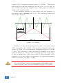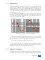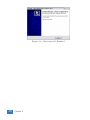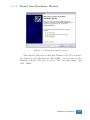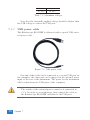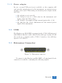
1
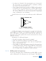
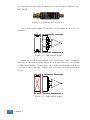
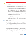
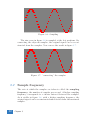
Handyscope HS4 DIFF
User manual
TiePie engineering
ATTENTION!
Measuring directly on the line voltage can be very dangerous.
Copyright c 2014 TiePie engineering.
All rights reserved.
Revision 2.9, October 2014
Despite the care taken for the compilation of this
user manual, TiePie engineering can not be held
responsible for any damage resulting from errors
that may appear in this manual.
Contents
1 Safety
1
2 Declaration of conformity
3
3 Introduction
3.1 Differential input . . . . . . . .
3.1.1 Differential attenuators
3.1.2 Differential test lead . .
3.2 Sampling . . . . . . . . . . . .
3.3 Sample frequency . . . . . . . .
3.3.1 Aliasing . . . . . . . . .
3.4 Digitizing . . . . . . . . . . . .
3.5 Signal coupling . . . . . . . . .
.
.
.
.
.
.
.
.
.
.
.
.
.
.
.
.
.
.
.
.
.
.
.
.
.
.
.
.
.
.
.
.
.
.
.
.
.
.
.
.
.
.
.
.
.
.
.
.
.
.
.
.
.
.
.
.
.
.
.
.
.
.
.
.
.
.
.
.
.
.
.
.
.
.
.
.
.
.
.
.
.
.
.
.
.
.
.
.
5
6
7
9
9
10
11
13
13
.
.
.
.
.
.
.
.
4 Driver installation
15
4.1 Introduction . . . . . . . . . . . . . . . . . . . . . . . 15
4.2 Where to find the driver setup . . . . . . . . . . . . 15
4.3 Executing the installation utility . . . . . . . . . . . 15
5 Hardware installation
5.1 Power the instrument . . . . . . . . . .
5.1.1 External power . . . . . . . . . .
5.2 Connect the instrument to the computer
5.2.1 Found New Hardware Wizard . .
5.3 Plug into a different USB port . . . . .
.
.
.
.
.
.
.
.
.
.
.
.
.
.
.
.
.
.
.
.
.
.
.
.
.
.
.
.
.
.
.
.
.
.
.
21
21
21
22
23
25
6 Front panel
27
6.1 Channel input connectors . . . . . . . . . . . . . . . 27
6.2 Power indicator . . . . . . . . . . . . . . . . . . . . . 27
7 Rear panel
7.1 Power . . . . . . . . . .
7.1.1 USB power cable
7.1.2 Power adapter .
7.2 USB . . . . . . . . . . .
7.3 Extension Connector . .
.
.
.
.
.
.
.
.
.
.
.
.
.
.
.
.
.
.
.
.
.
.
.
.
.
.
.
.
.
.
.
.
.
.
.
.
.
.
.
.
.
.
.
.
.
.
.
.
.
.
.
.
.
.
.
.
.
.
.
.
.
.
.
.
.
.
.
.
.
.
8 Specifications
.
.
.
.
.
.
.
.
.
.
29
29
30
31
31
31
33
Contents
I
8.1
8.2
8.3
8.4
8.5
8.6
8.7
8.8
8.9
8.10
8.11
II
Acquisition system . . . . . . .
BNC inputs CH1 to CH4 . . .
Trigger system . . . . . . . . .
Interface . . . . . . . . . . . . .
Power . . . . . . . . . . . . . .
Physical . . . . . . . . . . . . .
I/O connectors . . . . . . . . .
System requirements . . . . . .
Environmental conditions . . .
Certifications and Compliances
Package contents . . . . . . . .
.
.
.
.
.
.
.
.
.
.
.
.
.
.
.
.
.
.
.
.
.
.
.
.
.
.
.
.
.
.
.
.
.
.
.
.
.
.
.
.
.
.
.
.
.
.
.
.
.
.
.
.
.
.
.
.
.
.
.
.
.
.
.
.
.
.
.
.
.
.
.
.
.
.
.
.
.
.
.
.
.
.
.
.
.
.
.
.
.
.
.
.
.
.
.
.
.
.
.
.
.
.
.
.
.
.
.
.
.
.
.
.
.
.
.
.
.
.
.
.
.
.
.
.
.
.
.
.
.
.
.
.
33
33
34
34
34
34
34
35
35
35
35
Safety
1
When working with electricity, no instrument can guarantee complete safety. It is the responsibility of the person
who works with the instrument to operate it in a safe way.
Maximum security is achieved by selecting the proper instruments and following safe working procedures. Safe
working tips are given below:
• Always work according (local) regulations.
• Work on installations with voltages higher than 25 VAC or
60 VDC should only be performed by qualified personnel.
• Avoid working alone.
• Observe all indications on the Handyscope HS4 DIFF before
connecting any wiring
• Check the probes/test leads for damages. Do not use them
if they are damaged
• Take care when measuring at voltages higher than 25 VAC or
60 VDC .
• Do not operate the equipment in an explosive atmosphere or
in the presence of flammable gases or fumes.
• Do not use the equipment if it does not operate properly.
Have the equipment inspected by qualified service personal.
If necessary, return the equipment to TiePie engineering for
service and repair to ensure that safety features are maintained.
Safety
1
2
Chapter 1
Declaration of conformity
2
TiePie engineering
Koperslagersstraat 37
8601 WL Sneek
The Netherlands
EC Declaration of conformity
We declare, on our own responsibility, that the product
Handyscope
Handyscope
Handyscope
Handyscope
HS4
HS4
HS4
HS4
DIFF-5MHz
DIFF-10MHz
DIFF-25MHz
DIFF-50MHz
for which this declaration is valid, is in compliance with
EN 55011:2009/A1:2010
EN 55022:2006/A1:2007
IEC 61000-6-1/EN 61000-6-1:2007
IEC 61000-6-1/EN 61000-6-1:2007
according the conditions of the EMC standard 2004/108/EC
and also with
Canada: ICES-001:2004
Australia/New Zealand: AS/NZS
Sneek, 1-11-2010
ir. A.P.W.M. Poelsma
Declaration of conformity
3
Environmental considerations
This section provides information about the environmental impact
of the Handyscope HS4 DIFF.
Handyscope HS4 DIFF end-of-life handling
Production of the Handyscope HS4 DIFF required the extraction
and use of natural resources. The equipment may contain substances that could be harmful to the environment or human health
if improperly handled at the Handyscope HS4 DIFF’s end of life.
In order to avoid release of such substances into the environment
and to reduce the use of natural resources, recycle the Handyscope
HS4 DIFF in an appropriate system that will ensure that most of
the materials are reused or recycled appropriately.
The symbol shown below indicates that the Handyscope HS4
DIFF complies with the European Union’s requirements according
to Directive 2002/96/EC on waste electrical and electronic equipment (WEEE).
Restriction of Hazardous Substances
The Handyscope HS4 DIFF has been classified as Monitoring and
Control equipment, and is outside the scope of the 2002/95/EC
RoHS Directive.
4
Chapter 2
3
Introduction
Before using the Handyscope HS4 DIFF first read chapter 1
about safety.
Many technicians investigate electrical signals. Though the
measurement may not be electrical, the physical variable is often converted to an electrical signal, with a special transducer.
Common transducers are accelerometers, pressure probes, current
clamps and temperature probes. The advantages of converting the
physical parameters to electrical signals are large, since many instruments for examining electrical signals are available.
The Handyscope HS4 DIFF is a portable four channel measuring instrument with differential inputs. The Handyscope HS4 DIFF
is available in several models with different maximum sampling frequencies. The native resolution is 12 bits, but user selectable resolutions of 14 and 16 bits are available too, with reduced maximum
sampling frequency:
resolution
Model 50
Model 25
Model 10
Model 5
12 bit
14 bit
16 bit
50 MS/s
3.125 MS/s
25 MS/s
3.125 MS/s
10 MS/s
3.125 MS/s
5 MS/s
3.125 MS/s
195 kS/s
195 kS/s
195 kS/s
195 kS/s
Table 3.1: Maximum sampling frequencies
The Handyscope HS4 DIFF supports high speed continuous
streaming measurements. The maximum streaming rates are:
resolution
Model 50
Model 25
Model 10
Model 5
12 bit
500 kS/s
250 kS/s
100 kS/s
50 kS/s
14 bit
16 bit
480 kS/s
195 kS/s
250 kS/s
195 kS/s
99 kS/s
97 kS/s
50 kS/s
48 kS/s
Table 3.2: Maximum streaming rates
Introduction
5
With the accompanying software the Handyscope HS4 DIFF
can be used as an oscilloscope, a spectrum analyzer, a true RMS
voltmeter or a transient recorder. All instruments measure by sampling the input signals, digitizing the values, process them, save
them and display them.
3.1 Differential input
Most oscilloscopes are equipped with standard, single ended inputs,
which are referenced to ground. This means that one side of the
input is always connected to ground and the other side to the point
of interest in the circuit under test.
Figure 3.1: Single ended input
Therefore the voltage that is measured with an oscilloscope with
standard, single ended inputs is always measured between that
specific point and ground.
When the voltage is not referenced to ground, connecting a
standard single ended oscilloscope input to the two points would
create a short circuit between one of the points and ground, possibly damaging the circuit and the oscilloscope.
A safe way would be to measure the voltage at one of the two
points, in reference to ground and at the other point, in reference to
ground and then calculate the voltage difference between the two
points. On most oscilloscopes this can be done by connecting one
of the channels to one point and another channel to the other point
and then use the math function CH1 - CH2 in the oscilloscope to
display the actual voltage difference.
There are some disadvantages to this method:
• a short circuit to ground can be created when an input is
wrongly connected
• to measure one signal, two channels are occupied
6
Chapter 3
• by using two channels, the measurement error is increased,
the errors made on each channel will be combined, resulting
in a larger total measurement error
• The Common Mode Rejection Ratio (CMRR) of this method
is relatively low. If both points have a relative high voltage,
but the voltage difference between the two points is small,
the voltage difference can only be measured in a high input
range, resulting in a low resolution
A much better way is to use an oscilloscope with a differential
input.
Figure 3.2: Differential input
A differential input is not referenced to ground, but both sides
of the input are ”floating”. It is therefore possible to connect one
side of the input to one point in the circuit and the other side of
the input to the other point in the circuit and measure the voltage
difference directly.
Advantages of a differential input:
• No risk of creating a short circuit to ground
• Only one channel is required to measure the signal
• More accurate measurements, since only one channel introduces a measurement error
• The CMRR of a differential input is high. If both points have
a relative high voltage, but the voltage difference between the
two points is small, the voltage difference can be measured
in a low input range, resulting in a high resolution
3.1.1
Differential attenuators
To increase the input range of the Handyscope HS4 DIFF, it comes
with a differential 1:10 attenuator for each channel. This differenIntroduction
7
tial attenuator is specially designed to be used with the Handyscope
HS4 DIFF.
Figure 3.3: Differential attenuator
For a differential input, both sides of the input need to be attenuated.
Figure 3.4: Differential input
Standard oscilloscope probes and attenuators only attenuate
one side of the signal path. These are not suitable to be used with
a differential input. Using these on a differential input will have
a negative effect on the CMRR and will introduce measurement
errors.
Figure 3.5: Differential input
8
Chapter 3
The Differential Attenuator and the inputs of the Handyscope HS4 Diff are differential, which means that the outside
of the BNC’s are not grounded, but carry life signals.
When using the attenuator, the following points have to be
taken into consideration:
• do not connect other cables to the attenuator than the ones
that are supplied with the instrument
• do not touch the metal parts of the BNC’s when the attenuator is connected to the circuit under test, they can carry
a dangerous voltage. It will also influence the measurements
and create measurement errors.
• do not connect the outside of the two BNC’s of the attenuator
to each other as this will short circuit a part of the internal
circuit and will create measurement errors
• do not connect the outside of the BNC’s of two or more attenuators that are connected to different channels of the Handyscope HS4 Diff to each other
• do not apply excessive mechanical force to the attenuator in
any direction (e.g. pulling the cable, using the attenuator as
handle to carry the Handyscope HS4 DIFF, etc.)
3.1.2
Differential test lead
The Handyscope HS4 DIFF comes with a special differential test
lead. This test lead is specially designed to ensure a good CMRR.
The special heat resistant differential test lead provided with
the Handyscope HS4 DIFF is designed to be immune for noise
from the surrounding environment.
3.2 Sampling
When sampling the input signal, samples are taken at fixed intervals. At these intervals, the size of the input signal is converted to a
number. The accuracy of this number depends on the resolution of
the instrument. The higher the resolution, the smaller the voltage
steps in which the input range of the instrument is divided. The
acquired numbers can be used for various purposes, e.g. to create
a graph.
Introduction
9
Figure 3.6: Sampling
The sine wave in figure 3.6 is sampled at the dot positions. By
connecting the adjacent samples, the original signal can be reconstructed from the samples. You can see the result in figure 3.7.
Figure 3.7: ”connecting” the samples
3.3 Sample frequency
The rate at which the samples are taken is called the sampling
frequency, the number of samples per second. A higher sampling
frequency corresponds to a shorter interval between the samples.
As is visible in figure 3.8, with a higher sampling frequency, the
original signal can be reconstructed much better from the measured
samples.
10
Chapter 3
Figure 3.8: The effect of the sampling frequency
The sampling frequency must be higher than 2 times the highest frequency in the input signal. This is called the Nyquist frequency. Theoretically it is possible to reconstruct the input signal
with more than 2 samples per period. In practice, 10 to 20 samples per period are recommended to be able to examine the signal
thoroughly.
3.3.1
Aliasing
When sampling an analog signal with a certain sampling frequency,
signals appear in the output with frequencies equal to the sum and
difference of the signal frequency and multiples of the sampling
frequency. For example, when the sampling frequency is 1000 Hz
and the signal frequency is 1250 Hz, the following signal frequencies
will be present in the output data:
Multiple of sampling frequency
1250 Hz signal
-1250 Hz signal
-1000
-1000 + 1250 = 250
-1000 - 1250 = -2250
0
0 + 1250 = 1250
1000
1000 + 1250 = 2250
1000 - 1250 =
-250
2000
2000 + 1250 = 3250
2000 - 1250 =
750
...
0 - 1250 = -1250
...
Table 3.3: Aliasing
As stated before, when sampling a signal, only frequencies lower
than half the sampling frequency can be reconstructed. In this
case the sampling frequency is 1000 Hz, so we can we only observe
Introduction
11
signals with a frequency ranging from 0 to 500 Hz. This means
that from the resulting frequencies in the table, we can only see
the 250 Hz signal in the sampled data. This signal is called an
alias of the original signal.
If the sampling frequency is lower than twice the frequency of
the input signal, aliasing will occur. The following illustration
shows what happens.
Figure 3.9: Aliasing
In figure 3.9, the green input signal (top) is a triangular signal
with a frequency of 1.25 kHz. The signal is sampled with a frequency of 1 kHz. The corresponding sampling interval is 1/1000Hz
= 1ms. The positions at which the signal is sampled are depicted
with the blue dots. The red dotted signal (bottom) is the result
of the reconstruction. The period time of this triangular signal
appears to be 4 ms, which corresponds to an apparent frequency
(alias) of 250 Hz (1.25 kHz - 1 kHz).
To avoid aliasing, always start measuring at the highest sampling frequency and lower the sampling frequency if required.
12
Chapter 3
3.4 Digitizing
When digitizing the samples, the voltage at each sample time is
converted to a number. This is done by comparing the voltage
with a number of levels. The resulting number is the number corresponding to the level that is closest to the voltage. The number
of levels is determined by the resolution, according to the following
relation: LevelCount = 2Resolution .
The higher the resolution, the more levels are available and
the more accurate the input signal can be reconstructed. In figure
3.10, the same signal is digitized, using two different amounts of
levels: 16 (4-bit) and 64 (6-bit).
Figure 3.10: The effect of the resolution
The Handyscope HS4 DIFF measures at e.g. 12 bit resolution
(212 =4096 levels). The smallest detectable voltage step depends
on the input range. This voltage can be calculated as:
V oltageStep = F ullInputRange/LevelCount
For example, the 200 mV range ranges from -200 mV to +200
mV, therefore the full range is 400 mV. This results in a smallest
detectable voltage step of 0.400V/4096 = 97.65 µV.
3.5 Signal coupling
The Handyscope HS4 DIFF has two different settings for the signal
coupling: AC and DC. In the setting DC, the signal is directly
Introduction
13
coupled to the input circuit. All signal components available in the
input signal will arrive at the input circuit and will be measured.
In the setting AC, a capacitor will be placed between the input
connector and the input circuit. This capacitor will block all DC
components of the input signal and let all AC components pass
through. This can be used to remove a large DC component of the
input signal, to be able to measure a small AC component at high
resolution.
When measuring DC signals, make sure to set the signal
coupling of the input to DC.
14
Chapter 3
4
Driver installation
Before connecting the Handyscope HS4 DIFF to the computer, the drivers need to be installed.
4.1 Introduction
To operate a Handyscope HS4 DIFF, a driver is required to interface between the measurement software and the instrument. This
driver takes care of the low level communication between the computer and the instrument, through USB. When the driver is not
installed, or an old, no longer compatible version of the driver is
installed, the software will not be able to operate the Handyscope
HS4 DIFF properly or even detect it at all.
The installation of the USB driver is done in a few steps. Firstly,
the driver has to be pre-installed by the driver setup program. This
makes sure that all required files are located where Windows can
find them. When the instrument is plugged in, Windows will detect
new hardware and install the required drivers.
4.2 Where to find the driver setup
The driver setup program and measurement software can be found
in the download section on TiePie engineering’s website and on the
CD-ROM that came with the instrument. It is recommended to
install the latest version of the software and USB driver from the
website. This will guarantee the latest features are included.
4.3 Executing the installation utility
To start the driver installation, execute the downloaded driver
setup program, or the one on the CD-ROM that came with the
instrument. The driver install utility can be used for a first time
Driver installation
15
installation of a driver on a system and also to update an existing
driver.
The screen shots in this description may differ from the ones
displayed on your computer, depending on the Windows version.
Figure 4.1: Driver install: step 1
When drivers were already installed, the install utility will remove them before installing the new driver. To remove the old
driver successfully, it is essential that the Handyscope HS4 DIFF
is disconnected from the computer prior to starting the driver install utility. When the Handyscope HS4 DIFF is used with an
external power supply, this must be disconnected too.
16
Chapter 4
Figure 4.2: Driver install: step 2
When the instrument is still connected, the driver install utility
will recognize it and report this. You will be asked to continue
anyway.
Figure 4.3: Driver install: Instrument is still connected
Clicking ”No” will bring back the previous screen. The instrument should now be disconnected. Then the removal of the existing
driver can be continued by clicking ”Next”.
Clicking ”Yes” will ignore the fact that the instrument is still
connected and continue removal of the old driver. This option is
not recommended, as removal may fail, after which installation of
the new driver may fail as well.
When no existing driver was found or the existing driver is
removed, the location for the pre-installation of the new driver can
be selected.
Driver installation
17
Figure 4.4: Driver install: step 3
On Windows XP and newer, the installation may inform about
the drivers not being ”Windows Logo Tested”. The driver is not
causing any danger for your system and can be safely installed.
Please ignore this warning and continue the installation.
Figure 4.5: Driver install: step 4
The driver install utility now has enough information and can
install the drivers. Clicking ”Install” will remove existing drivers
and install the new driver. A remove entry for the new driver is
added to the software applet in the Windows control panel.
18
Chapter 4
Figure 4.6: Driver install: step 5
As mentioned, Windows XP SP2 and newer may warn for the
USB drivers not being Windows Logo tested. Please ignore this
warning and continue anyway.
Figure 4.7: Driver install: Ignore warning and continue
Driver installation
19
Figure 4.8: Driver install: Finished
20
Chapter 4
Hardware installation
5
Drivers have to be installed before the Handyscope HS4
DIFF is connected to the computer for the first time. See
chapter 4 for more information.
5.1 Power the instrument
The Handyscope HS4 DIFF is powered by the USB, no external
power supply is required. Only connect the Handyscope HS4 DIFF
to a bus powered USB port, otherwise it may not get enough power
to operate properly.
5.1.1
External power
In certain cases, it can be that the Handyscope HS4 DIFF cannot
get enough power from the USB port.
When a Handyscope HS4 DIFF is connected to a USB port, the
hardware will be powered, resulting in an inrush current, which is
higher than the nominal current. After the inrush current, the
current will stabilize at the nominal current.
USB ports have a maximum limit for both the inrush current
peak and the nominal current. When either of them is exceeded,
the USB port will be switched off. As a result, the connection to
the Handyscope HS4 DIFF will be lost.
Most USB ports can supply enough current for the Handyscope
HS4 DIFF to work without an external power supply, but this is not
always the case. Some (battery operated) portable computers or
(bus powered) USB hubs do not supply enough current. The exact
value at which the power is switched off, varies per USB controller,
so it is possible that the Handyscope HS4 DIFF functions properly
on one computer, but does not on another.
In order to power the Handyscope HS4 DIFF externally, an
external power input is provided for. It is located at the rear of the
Hardware installation
21
Handyscope HS4 DIFF. Refer to paragraph 7.1 for specifications
of the external power intput.
5.2 Connect the instrument to the computer
After the new driver has been pre-installed (see chapter 4), the
Handyscope HS4 DIFF can be connected to the computer. When
the Handyscope HS4 DIFF is connected to a USB port of the computer, Windows will report new hardware. The Found New Hardware Wizard will appear.
Depending on the Windows version, the New Hardware Wizard
will show a number of screens in which it will ask for information
regarding the drivers of the newly found hardware. The appearance of the dialogs will differ for each Windows version and might
be different on the computer where the Handyscope HS4 DIFF is
installed.
The driver consists of two parts which are installed separately.
Once the first part is installed, the installation of the second
part will start automatically. Installation of the second part is
identical to the first part, therefore they are not described individually here.
22
Chapter 5
5.2.1
Found New Hardware Wizard
Figure 5.1: Hardware install: step 1
This window will only be shown in Windows XP SP2 or newer.
No drivers for the Handyscope HS4 DIFF can be found on the
Windows Update Web site, so select ”No, not this time” and
click ”Next”.
Hardware installation
23
Figure 5.2: Hardware install: step 2
Since the drivers are already pre-installed on the computer,
Windows will be able to find them automatically. Select ”Install
the software automatically” and click ”Next”.
Figure 5.3: Hardware install: step 3
The New Hardware wizard will now copy the required files to
their destination.
24
Chapter 5
Figure 5.4: Hardware install: step 4
The first part of the new driver is now installed. Click ”Finish”
to close the wizard and start installation of the second part, which
follows identical steps.
Once the second part of the driver is installed. measurement
software can be installed and the Handyscope HS4 DIFF can be
used.
5.3 Plug into a different USB port
When the Handyscope HS4 DIFF is plugged into a different USB
port, some Windows versions will treat the Handyscope HS4 DIFF
as different hardware and will ask to install the drivers again. This
is controlled by Microsoft Windows and is not caused by TiePie
engineering.
Hardware installation
25
26
Chapter 5
6
Front panel
Figure 6.1: Front panel
6.1 Channel input connectors
The CH1 – CH4 BNC connectors are the main inputs of the acquisition system. The isolated BNC connectors are not connected to
the ground of the Handyscope HS4 DIFF.
6.2 Power indicator
A power indicator is situated at the top cover of the instrument.
It is lit when the Handyscope HS4 DIFF is powered.
Front panel
27
28
Chapter 6
7
Rear panel
Figure 7.1: Rear panel
7.1 Power
The Handyscope HS4 DIFF is powered through the USB. If the
USB cannot deliver enough power, it is possible to power the instrument externally. The Handyscope HS4 DIFF has two external
power inputs located at the rear of the instrument: the dedicated
power input and a pin of the extension connector.
The specifications of the dedicated power connector are:
Pin
Center pin
Outside bushing
Dimension
Ø1.3 mm
Ø3.5 mm
Description
ground
positive
Figure 7.2: Power connector
Besides the external power input, it is also possible to power
the instrument through the extension connector, the 25 pin D-sub
connector at the rear of the instrument. The power has to be
applied to pin 3 of the extension connector. Pin 4 can be used as
ground.
The following minimum and maximum voltages apply to both
power inputs:
Rear panel
29
Minimum
Maximum
4.5 VDC
14 VDC
Table 7.1: Maximum voltages
Note that the externally applied voltage should be higher than
the USB voltage to relieve the USB port.
7.1.1
USB power cable
The Handyscope HS4 DIFF is delivered with a special USB external power cable.
Figure 7.3: USB power cable
One end of this cable can be connected to a second USB port on
the computer, the other end can be plugged in the external power
input at the rear of the instrument. The power for the instrument
will be taken from two USB ports of the computer.
The outside of the external power connector is connected to
+5 V. In order to avoid shortage, first connect the cable to
the Handyscope HS4 DIFF and then to the USB port.
30
Chapter 7
7.1.2
Power adapter
In case a second USB port is not available, or the computer still
can’t provide enough power for the instrument, an external power
adapter can be used. When using an external power adapter, make
sure that:
• the polarity is set correctly
• the voltage is set to a valid value for the instrument and
higher than the USB voltage
• the adapter can supply enough current (preferably >1 A)
• the plug has the correct dimensions for the external power
input of the instrument
7.2 USB
The Handyscope HS4 DIFF is equipped with a USB 2.0 High speed
(480 Mbit/s) interface with a fixed cable with type A plug. It will
also work on a computer with a USB 1.1 interface, but will then
operate at 12 Mbit/s.
7.3 Extension Connector
Figure 7.4: Extension connector
To connect to the Handyscope HS4 DIFF a 25 pin female D-sub
connector is available, containing the following signals:
Rear panel
31
Pin
Description
Pin
Description
1
2
3
Ground
Reserved
External Power in DC
14
15
16
Ground
Ground
Reserved
4
5
6
7
8
9
Ground
+5V out, 10 mA max.
Ext. sampling clock in (TTL)
Ground
Ext. trigger in (TTL)
Data OK out (TTL)
17
18
19
20
21
22
Ground
Reserved
Reserved
Reserved
Reserved
Ground
Ground
Trigger out (TTL)
Reserved
Ext. sampling clock out (TTL)
23
24
25
I2 C SDA
I2 C SCL
Ground
10
11
12
13
Table 7.2: Pin description Extension connector
All TTL signals are 3.3 V TTL signals which are 5 V tolerant,
so they can be connected to 5 V TTL systems.
Pins 9, 11, 12, 13 are open collector outputs. Connect a pull-up
resistor of 1 kOhm to pin 5 when using one of these signals.
32
Chapter 7
8
Specifications
8.1 Acquisition system
Number of input channels
CH1, CH2, CH3, CH4
Maximum sampling rate
12 bit
14 bit
16 bit
Maximum streaming rate
12 bit
14 bit
16 bit
Sampling source
Internal
Accuracy
Stability
External
Voltage
Frequency range
Memory
4 analog
isolated BNC
depending on model
50 MS/s, 25 MS/s, 10 MS/s or 5 MS/s
3.125 MS/s
195 kS/s
depending on model
500 kS/s, 250 kS/s, 100 kS/s or 50 kS/s
480 kS/s, 250 kS/s, 99 kS/s or 50 kS/s
195 kS/s, 195 kS/s, 97 kS/s or 48 kS/s
internal quartz, external
Quartz
±0.01%
±100 ppm over -40◦ C to +85◦ C
On extension connector
3.3 V TTL, 5 V TTL tolerant
95 MHz to 105 MHz
128 kSamples per channel
8.2 BNC inputs CH1 to CH4
Type
Differential
Resolution
12, 14, 16 bit user selectable
Accuracy
0.3% of full scale ± 1 LSB
Range
200 mV to 80 V full scale
Coupling
AC/DC
Impedance
1 MΩ / 30 pF
Maximum voltage
200 V (DC + AC peak <10 kHz)
Maximum voltage with 1:10 attenuator500 V (DC + AC peak <10 kHz)
Maximum common mode voltage
200 mV to 800 mV ranges : 2 V
2 V to 8 V ranges : 20 V
20 V to 80 V ranges : 200 V
Common Mode Rejection Ratio
-48 dB
Channel Isolation
500 V
Channel Separation
-80 dB
Bandwidth (-3dB)
50 MHz
AC coupling cut off frequency (-3dB) ±1.5 Hz
Specifications
33
8.3 Trigger system
System
Source
Trigger modes
Level adjustment
Hysteresis adjustment
Resolution
Pre trigger
Post trigger
Digital external trigger
Input
Range
Coupling
digital, 2 levels
CH1, CH2, CH3, CH4, digital external, AND, OR
rising slope, falling slope,
inside window, outside window
0 to 100% of full scale
0 to 100% of full scale
0.024 % (12 bits)
0 to 128 ksamples (0 to 100%, one sample resolution)
0 to 128 ksamples (0 to 100%, one sample resolution)
extension connector
0 to 5 V (TTL)
DC
8.4 Interface
Interface
USB 2.0 High Speed (480 Mbit/s)
(USB 1.1 Full Speed (12 Mbit/s) compatible)
8.5 Power
Input
Consumption
from USB or external input
500 mA max
8.6 Physical
Instrument height
Instrument length
Instrument width
Weight
USB cord length
25 mm / 1.0”
170 mm / 6.7”
140 mm / 5.2”
480 gram / 17 ounce
1.8 m / 70”
8.7 I/O connectors
CH1 .. CH4
Power
Extension connector
USB
34
Chapter 8
BNC
3.5 mm power socket
D-sub 25 pins female
Fixed cable with type A plug
8.8 System requirements
PC I/O connection
Operating System
USB 2.0 High Speed (480 Mbit/s)
(USB 1.1 Full Speed (12 Mbit/s) compatible)
Windows 98/ME/2000/XP/Vista/7
8.9 Environmental conditions
Operating
Ambient temperature
Relative humidity
Storage
Ambient temperature
Relative humidity
0◦ C to 55◦ C
10 to 90% non condensing
-20◦ C to 70◦ C
5 to 95% non condensing
8.10 Certifications and Compliances
CE mark compliance
RoHS
Yes
Yes
8.11 Package contents
Instrument
Test lead
Accessories
Software
Drivers
Manual
Handyscope HS4 DIFF
4 x low noise differential with 4 mm banana jacks
4 x 1:10 differential attenuators
USB power cable
Windows 98/2000/ME/XP/Vista/7
Windows 98/2000/ME/XP/Vista/7
Instrument manual and software user’s manual
Specifications
35
36
Chapter 8
If you have any suggestions and/or remarks regarding this manual, please
contact:
@
TiePie engineering
P.O. Box 290
8600 AG SNEEK
The Netherlands
@ TiePie engineering
Koperslagersstraaat 37
8601 WL SNEEK
The Netherlands
Tel.:
Fax:
E-mail:
Site:
+31 515 415 416
+31 515 418 819
[email protected]
www.tiepie.nl