Download Spectra-L200 - JTW Astronomy

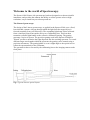
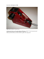
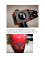
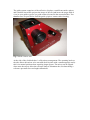
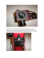
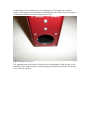
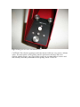
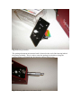
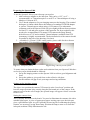
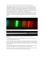
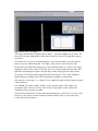
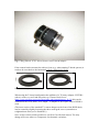
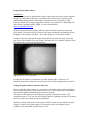
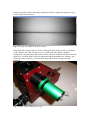
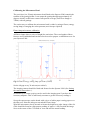
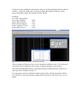
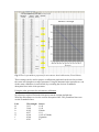
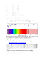
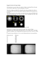
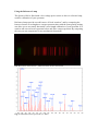
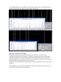
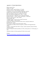
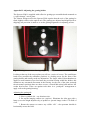
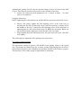
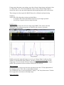
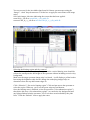
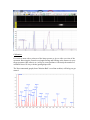
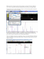
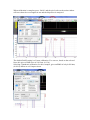
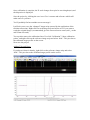
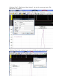
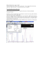
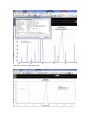
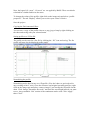
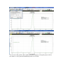
Spectra-L200
Users Manual for the Spectra L200
JTW Astronomy
Revised : June 2014
Welcome to the world of Spectroscopy!
The Spectra-L200 Littrow slit spectroscope has been designed as a robust scientific
instrument, and provides the amateur the ability to collect spectra at low or high
resolution, easy to install on your telescope and use.
The Littrow Spectroscope
The design of the Littrow spectroscope, as applied in the Spectra-L200, uses a fixed,
but selectable, entrance slit gap through which the light from the target object is
focused (normally from your telescope). The expanding light beam is then reflected
from a small precision front surface mirror to a collimating lens. This lens then
transmits a parallel light bundle to the reflective diffraction grating. The grating
generates a series of spectra. The precision grating used in the Spectra-L200 has a
“blazed” profile to maximise the light dispersed into the resulting spectrum. To record
different target wavelengths within the spectrum, the grating can be rotated using a
precision micrometer. The grating holder is set at a slight angle to the optical axis to
reflect the spectrum back to the collimator.
The spectrum is then re-focused by the collimating lens to the imaging camera at the
focal plane.
Fig 1 Typical Littrow optical layout
Overview of the Spectra-L200
Fig 2 Spectra-L200 – General View
Starting at the front, we have the inlet port. This has a female T thread connection and
your telescope nosepiece/ adaptor should be fitted here.
When you look inside you see the reflective guide/ slit arrangement.
Fig 3 Inlet port showing slit plate (reference mirror retracted)
The slit gap, visible as a thin black line in the mirror surface (and the selection
number) should be seen in the middle. The front protective plate provides a clear
guide aperture of 7mm x 20mm. There are 12 slit/ pinhole options available, selected
by turning the external thumbwheel. The index detent maintains the slit gap on the
optical axis.
Fig 4 Thumbwheel indexing for slit gap
The guide system comprises of the reflective slit plate, a small front surface mirror
and a doublet lens which projects the image of the slit (and hence the target field of
view) to your guide eyepiece (or guide camera) located in the external holder. Two
thumbscrews are provided to lock the guide eyepiece/ camera after focusing.
Fig 5 Guide camera tube
At the side of the slit block there’s a flip mirror arrangement. The actuating knob on
the side allows this mirror to be retracted (held in place with a small magnetic catch) –
this is its normal position when acquiring target spectra. The mirror can be flipped
down onto the stop to allow the reference lamp to illuminate the slit when taking a
reference spectrum for wavelength calibrations.
Fig 6 Inlet port showing reference mirror in position
Mounted on the outside surface of the housing is the reference lamp assembly. This
holds the power electronics for the reference lamp (interchangeable) which is
mounted at the top. The lamp illuminates a small aperture which is then, via the flip
mirror, projected to the slit gap. This module needs a 12V power supply. This should
be a 2.1/5.5mm centre positive 12VDC supply. (Supplied by user)
Fig 7 Reference lamp and driver
At the bottom of the housing, there’s the imaging port. This again has a female T
thread. Your imaging camera should be mounted to this port. The back focus distance
is 60mm (the distance from the housing to the CCD)
Fig 8 Imaging camera port
The grating assembly which has various screws for adjustment is held in place on the
housing by three large thumbscrews. Removing these thumbscrews allows the grating
to be removed/ replaced.
Fig 9 Grating access cover and thumbscrews
CAUTION: The reflective gratings used in the Spectra-L200 are very precise, delicate
optics. The front surface of the grating must be protected at all times and never
touched with the fingers. Any finger prints, marks etc. are impossible to remove and
can seriously affect the performance of the grating. DON’T TOUCH.
Fig 10 Grating assembly
The grating adjustment micrometer head is located on the end of the housing behind
the grating assembly. This is used to rotate the grating in its holder to bring the
required target wavelength into the imaging camera field of view.
Fig 11 Grating adjustment micrometer head
Preparing the Spectra-L200
To use the Spectra-L200 on your telescope you need to:
1. Add a telescope adaptor to the inlet port. This can be a 1.25” (or 2” –
recommended) to T thread nosepiece or an SCT to T thread adaptor if using a
Meade or Celestron SCT.
2. Use T thread adaptors to fit your imaging camera to the housing. The nominal
backspace is 60mm which allows the fitment of a standard T2 DSLR adaptor
or various T thread spacers when using a CCD camera. The achromatic
collimator used in the Spectra-L200 will give slightly different focus positions
for blue/UV, red and green regions of the spectrum. For best resolution, this
needs to be accommodated. For normal CCD cameras the Borg/ Hutech
helical focuser #7315 and a suitable T thread adaptor (available from JTW
Astronomy) is highly recommended. The horizontal axis of the camera should
lie parallel to the base of the housing. (See later)
3. A suitable 2.1/5.5mm 12VDC centre positive power cable for the reference
lamp module. This should be rated for 1A.
Fig 12 2” nosepiece fitted
Fig 13 Borg camera focuser fitted
To ensure that you obtain the best results and resolution from your Spectra-L200 there
are few key steps which should be followed.
a. Set up the imaging camera on the Spectra-L200 to achieve good alignment and
focus
b. Set-up the guider to give good focus on the reflective slit plate
c. Set the entrance slit gap to suit your target and seeing conditions
Setting up the imaging camera
The object is to position the camera CCD securely at the “best focus” position and
have the target spectrum lying exactly along the horizontal axis of the camera. If the
camera is not set at the correct angle, the spectral image will appear “tilted” across the
field of view.
Setting the camera focus
This is initially best done on the bench. You need to illuminate the entrance slit with a
suitable light source. A piece of greaseproof paper/ tracing paper over the inlet port
gives a good diffuse light. As you’ll probably be moving on to calibrating the grating
rotation, use an energy saving fluoro lamp. Position the lamp a metre or so from the
inlet port such that it fully illuminates the slit.
The entrance slit gap, should be set reasonable narrow (around 29 micron).
The adaptors necessary to set the camera CCD at or close to the design back focal
position should already be in place. Provision for camera rotation (to reduce “tilt”)
should also be available. I also strongly recommend that you orientate the spectrum
central to your CCD frame and horizontal across the larger axis. This reduces the
“tilt” angle and possible loss of resolution. (The absorption/ emission lines within the
spectrum height will probably end up showing a “slant” where the
absorption/emission lines look “slanted” relative to the spectrum. This is normal. It
can easily be corrected in your normal processing. Do NOT be tempted to align the
absorption/ emission line vertically….get the spectrum horizontal across the CCD
chip.)
Fig 14 Spectral image showing tilt across the CCD
Fig 15 Spectrum corrected for tilt – showing the slant of the lines within the
spectrum\
Set up the camera to give a 0.5 sec exposure (this will vary camera to camera, and
we’ll reset the exposure again later)
You can access the slit zero order image (by rotating the grating to a position where it
acts as a front surface mirror, approx 1450 on the micrometer) then use this setting for
the initial focusing. Otherwise adjust the grating rotation until you get an image of the
slit on the CCD.
Adjust the grating position to bring the image close to the middle of the frame. (This
may require fine adjustment of your grating tilt angle. See Appendix B).
Now vary the exposure to get a well exposed image of the slit (zero order) or a tight
clean emission line. Overexposing the image will swamp the detail.
Fig 16 Zero order slit Image
The image should show a bright vertical “band” – probably slightly out of focus. The
next job is to make adjustments of the camera spacers/ focuser to bring this image to
best focus.
Trial and error. If you use T-thread adaptors, you can rotate them to see the impact
(don’t worry too much about the “tilt” angle – this can be corrected at the end.)
By the time you finish, the slit gap (zero order) should appear as a clean, crisp, tight
bright line in the centre of the CCD chip. If you’re using a bright emission line, then
again this should appear regular, and the edges of the slit gap clean in sharp focus.
For normal CCD cameras the Borg/ Hutech helical focuser #7315 and a suitable T
thread adaptor (available from JTW Astronomy) is highly recommended
Note that the “sweet spot” i.e. a field of view within the depth of focus limit is around
10mm diameter.
For a DSLR, the frame width is 22mm. At the extreme edges of the image, the
spectrum will be well out of focus. This will severely impact on the clarity and
resolution of the spectrum recorded.
You need to take this into account when determining your “best focus” for your CCD.
Focus on your region of interest and accept that extreme edge of your frame may
record at a lesser resolution.
Fig 17 Borg/Hutech #7315 helical focuser and T thread adaptor
If the camera has been rotated to achieve focus (e.g. when rotating T thread spacers) it
needs to be reset back to the horizontal without changing the focus.
Fig
18 TST2We adaptor –front view
Fig 19 TST2We adaptor –rear view
When using the T thread configuration the addition of a TS rotary adaptor #TST2We
(above) works very well and only takes up 5.5mm of back focus.
(http://www.teleskop-express.de/shop/index.php?manufacturers_id=39) this can be
combined with a #TS-EOSs “zero length” T2 adaptor to save space when a DSLR is
used.
(The inner section of the standard T2 camera adapter on the front of the DSLR body
can be rotated by slightly loosening the three small grub screws (remember to
retighten them when you’re finished!!))
Once we have achieved this good focus it will be fixed for that camera. The only
change will occur when we compensate for chromatic variations.
Preparing the guide camera
Introduction
Guiding the telescope to maintain the image of the target star exactly on the entrance
slit gap (for maximum efficiency) is normally achieved by using a suitable guide
camera and guiding software which then communicates any corrections to the
telescope mount. Your image acquisition software (e.g. AstroArtV5, MaximDL etc.)
may include a guiding option. PHD2.3 is also recommended.
http://openphdguiding.org/
With the Spectra-L200 the highly reflective glass chromed slit plate provides the
guide image. Using the telescope focuser, the target star and the surrounding field is
brought to a focus on the slit plate – this is the image seen in the guide camera.
Using the telescope controls the target star should be positioned exactly on the slit
gap, close to the middle of the slit length. The target star (or a suitable field star close
by) can then be used for the guiding routine.
Fig 20 Guider view of slit plate
Usually the slit length is orientated to sit either along the RA or Dec axis. To
minimise unnecessary direction reversal corrections; the Dec alignment is preferred.
Setting the guide camera/ entrance slit focus.
Prior to using the guide system, it’s necessary to mount the guide camera and adjust
the focus and orientation of the camera field of view. This can be done on the bench
with subdued lighting illuminating the entrance slit plate.
The Spectra-L200 guide port is designed for a guide camera fitted with a 1.25”
standard nosepiece. You can use any suitable camera for guiding, but the SX Lodestar
camera is a proven performer and recommended.
With the reference flip mirror retracted, the reflective open area around the entrance
slit gap is visible to the guide camera. The transfer optics are designed to give
visibility to the maximum possible field of view.
Set up your guide camera and image acquisition software, adjust the exposure to give
a clear image of the slit area.
Fig 21 Slit gap from QHY5L II guide camera
Slide the guide camera nosepiece in/out of the guide tube until you can see an image
of the entrance slit. This will appear as a very fine dark line against a brighter
background. Carefully adjust the position of the camera to bring the line into clear and
tight focus. Lock the guide camera in position using the thumbscrews. Adding a par
focal ring to the nosepiece can be useful if the guide camera is being removed/
replaced.
Fig 22Guide camera and parfocal ring
To assist in positioning the target star on the slit gap, it is recommended that the guide
camera body be orientated to show the slit length sitting exactly horizontal or vertical
in the field of view.
The guide camera is now fixed and should not be moved.
These preliminary adjustments have been done in the comfort of your home. We need
now to consider the final steps needed to make the Spectra-L200 easy to use in the
“real life” situation – on a telescope, in the dark!
Preparing for spectral acquisition
The Spectra-L200 has to be configured to suit the project/ program being considered.
This entails:
1. Selection of the “best” grating/ SNR
2. Calibration of the micrometer head into wavelength settings
3. Selecting the optimum entrance slit gap for the telescope/ seeing conditions
4. Understanding the use of the reference lamp and acquiring reference spectra
The use of the SimSpecV4 spreadsheet is strongly recommended. This is available for
download from the JTW website or the Y! Group astronomical spectroscopy.
The spreadsheet allows you to enter the parameters of your telescope and camera etc.
and will assist in determining the optimum entrance slit gap, show the wavelength
coverage and resolution for the selected grating.
Grating selection
The grating is the heart of the spectroscope and the selection of the grating used will
have a significant impact on the brightness and resolution of the spectrum obtained.
Coarse gratings (150 l/mm and 300 l/mm) provide ideal low resolution (approx. 5.5A
with the 300 l/mm) spectra on faint objects or projects which require extended
spectral coverage.
As we increase the number of lines on the grating (600 l/mm or 1200 l/mm) the
resolution increases at the cost of reduced spectral coverage and when we use the high
resolution grating (1800 l/mm) the resolution will be better than 0.8A but with a much
reduced coverage – only 210A
SNR (Signal to noise ratio)
The quality of the spectrum produced is also measured in terms of the SNR.
This is directly related to the efficiency of your camera, the magnitude of the target
and obviously the total exposure time used. A minimum target SNR=20 should be
your goal, SNR>50 is a good result and SNR>200 is “ProAm” standard.
The use of the SimSpecV4 spreadsheet is strongly recommended to obtain a first
estimate of exposure times and probable SNR outcomes.
It’s recommended that you start out with a medium resolution grating. The 600 l/mm
grating is included as standard with the Spectra-L200.
With an ATik 314L camera and a ten minute exposure you will record ninth
magnitude star spectra with a good SNR (Signal to noise ratio) of around 50. The
wavelength coverage of the chip is approx. 720A and the resolution better than 2.7A.
The final spectrum will show sufficient detail for many projects.
Removing and replacing the gratings
The gratings supplied with the Spectra-L200 allow a wide range of low to high
resolutions and give differing wavelength coverage. The selection of the grating used
depends on the needs of the spectrum required (See above).
NOTE: Reflection gratings are very delicate and can easily be damaged. They should
never be handled at any time, and should be stored in dust tight containers when not
in use.
The gratings come pre-assembled in a rotating housing which is mounted on an access
plate. There are fine adjustment screws provided to ensure the tilt of the grating
holder matches the optical axis of the instrument. (Appendix B gives further detail on
these adjustments should they be necessary).
Changing over the grating is a simple and quick process. The micrometer head should
be adjusted to a reading of around 2000 (to release it from grating contact). The three
large Thumbscrews are then removed from the housing and the access cover complete
with grating can then be removed for safe storage.
Mounting a new grating is the reverse of the above. Again the micrometer head
should be withdrawn to a reading around 2000, the access cover positioned on the
housing and the three thumbscrews hand tightened.
Calibrating the Micrometer Head
The precision (0 to 25mm) micrometer head fitted to the Spectra-L200 controls the
rotation of the grating holder. It can rotate the grating through approximately 45
degrees which is sufficient to ensure full spectral coverage (from Zero Image to
7500A) with all gratings.
The easiest way to calibrate the micrometer head is either by using a fluoro (energy
saving lamp) or imaging the solar spectrum (no telescope required)
Fluoro lamp micrometer calibration
All fluoro lamps show a series of bright line emissions. The wavelengths of these
lines are well established and can therefore be used to prepare a calibration curve for
your Spectra-L200.
Fig 23 Fluoro energy saving lamp spectrum (C Buil)
Set the slit gap to say 39 micron (not critical).
The imaging camera should be fitted and focused on the Spectra-L200 (See Setting
the camera focus above ).
(Alternatively a 15mm eyepiece can be used in the imaging port if you have the
necessary adaptors. This is sufficiently accurate to get the necessary readings.)
Set up the spectroscope on the bench with a piece of white paper/ tracing paper over
the inlet port. Point the inlet port towards the Fluoro lamp.
Wind the micrometer slowly inwards to locate the bright zero order image of the slit.
(This should be found at a micrometer reading of approx. 1450) Position the image
close to the centre of the CCD field of view and note the actual reading.
Continue slowly winding the micrometer until you pick up the bright emission line in
the blue – centre the image and record the reading. Repeat this for the line in the
green, the double yellow line and the broader red line.
Example:
For a 600 l/mm grating
Zero Order (0000A)
Fluoro Blue (4358A)
Flouro Green (5461A)
Fluoro Yellow (5779A)
Fluoro Red (6113A)
1445
1255
1210
1195
1182
Fig 24 Yellow flouro doublet – 600 l/mm grating
These readings will form the basis of our instrument calibration curve. We will need
to generate a new calibration curve when we change gratings or micrometer.
The following illustration shows a typical micrometer calibration curve, based on a
solar spectrum. (Thanks to Frank J.)
It is important to do this calibration and keep the results with the instrument. When
you actually use the spectroscope at night on the telescope it will come in very, very
handy.
Fig 25 Excel spreadsheet prepared for micrometer head calibration (Frank Johns)
These settings can be used to prepare a calibration graph and can be used to position
the centre wavelength on a target spectrum. Using an annotated solar spectrum we can
do the same calibration, in more detail, by recording the obvious Fraunhofer
absorption lines in the solar spectrum.
Using the solar spectrum for micrometer calibration
No telescope required. Point the inlet port towards a bright daylight sky.
Wind the micrometer to view the various absorption lines. The prominent lines seen
are the Fraunhofer lines.
Line
K
H
h
g
G
f
e
Wavelength
3933
3968
4102
4227
4308
4340
4383
Source
Ca II
Ca II
H delta
Ca I
Ca/Fe (G Band)
H gamma
Fe
d
F
c
b2
b1
E
D2
D1
a band
C
B band
A band
4668
4861
4958
5173
5184
5269
5890
5896
6276-6287
6563
6867-6884
7594-7621
H beta
Fe I
Mg I
Mg I
Fe
Na I
Na I
H alpha
Atmospheric O2
Atmospheric O2
These are shown on the Liege solar spectral atlas
http://fermi.jhuapl.edu/liege/s00_0000.html
Fig 26 Liege solar spectrum
The highly detailed solar spectrum by Lunette Jean Rösch also highly recommended.
http://ljr.bagn.obs-mip.fr/observing/spectrum/
Fig 27 Typical high resolution solar spectrum
The above section shows the solar lines between 5800-5900 (Na doublet)
Even greater detail is given on the solar spectrum obtained on the BASS2000 website:
http://bass2000.obspm.fr/solar_spect.php?step=1
Suggested entrance slit gap settings
The thumbwheel is used to index the entrance slit plate, exposing different slit gaps.
You can select widths from 19 micron through to 96 micron
The choice of slit gap width will be dictated by the seeing conditions, the effective
focal length (EFL) of the telescope and the required resolution of the spectrum to be
recorded.
The normal slit gap selected would be just smaller than the anticipated FWHM (Full
width half maximum) size of the target star. The “excess” starlight at the sides of the
slit gap is used for guiding.
Fig 28 Details of slit gap/ pinhole v’s FWHM image (CAOS)
Shown above is a diagram of the typical star image (1a) a narrow slit gap
superimposed (1b) and a pinhole superimposed (1c). The residual “halo” is the light
available for guiding. The resulting light entering the spectroscope is shown in 1d and
1e.
For typical seeing conditions of 3 arc sec the following table gives some guidelines:
Slit gap (micron)
19
24
29
34
39
43
48
EFL(mm)
1500
1700
2000
2500
2750
3000
3600
Fig 29 Sample guider images showing target star being positioned close to slit gap
The SimSpecV4 spreadsheet can be used to generate results based on your actual
telescope and seeing conditions.
The width of the entrance slit also defines the quality of the spectrum produced.
The spectral image is made up of “strips” the width of which (related to the slit gap)
usually defines the wavelength resolution. To maximise the resolution and clarity of
the spectrum the imaging camera must have a pixel size less than 50% the slit gap.
For very faint stars, a large slit gap (>48 micron) will maximise the light throughput
but the resolution will be limited by the size of the seeing disk. This is called “slitless”
spectroscopy.
Focus the target (star) onto the entrance slit.
The guide camera must be focused on the slit gap before we start. (See previous
section)
The backfocus distance from the nosepiece adaptor to the entrance slit is 55mm; you
can first focus at this distance using an eyepiece on a suitable extension/ adaptor.
Start by using a bright star – they are easier to find (!) and give a bright zero order/
spectral image.
NOTE: You will not succeed in focusing your target star on a narrow (19 micron or
so) slit gap if your telescope and mount are not capable. The mount must be able to
hold all the equipment in a good balanced condition and be able to be guided to “lock
on” to the target star for at least 10-20 mins.
The telescope must be well collimated and the focuser robust enough to hold the
weight of the spectroscope and camera(s) with NO sag or movement.
With the spectroscope rigidly attached and the target star image in or very close to the
slit gap, adjust the focus to give the tightest star image you can get. If your guide
software has the capability of measuring the star size (FWHM) make use of it to find
the best focus. Use ONLY the focuser on the telescope. (Don’t touch the imaging
camera!)
Bring the target star image into the middle of the slit gap height. The closer the image
is to the center of the slit height, the closer it is to the optical axis (and the centre of
the CCD chip).
Take an exposure of the spectrum to confirm the star is actually there.
Move the star image from one side of the slit (using the fine controls on your mount)
to the other to ensure you are actually seeing the “central” core and not just one of the
edges. Take exposures after every adjustment. The height of the spectrum recorded
will depend on the seeing conditions; this size should be similar to the optimum
entrance slit gap used
Using the Reference Lamp
The Spectra-L200 is fitted with a low voltage power source to drive a reference lamp,
used for calibration of your spectrum.
Reference lamps provide a useful source of fixed “markers” and by comparing the
known reference wavelengths to a target spectrum taken with the same grating setting,
can allow you to accurately determine a wavelength calibration of your spectrum. It is
usual to take one reference spectrum before and after a target spectrum. By comparing
the two you can compensate for any mechanical distortions.
Fig 30 Typical Neon forest – emission lines in the red region
Fig 31 Annotated Neon spectrum (C. Buil)
The standard lamp uses a neon bulb. This provides a good series of defined reference
emission lines in the red region of the spectrum around Ha.
Fig 32 Neon reference lamp spectrum around 6200A – 600 l/mm grating
Fig 33 Neon spectrum around Ha region – 600 l/mm grating
Operation of the Reference lamp
The reference lamp is powered by a 240V circuit fed from a 12V DC source.
The On/Off switch powers the lamp. To obtain a reference spectrum, the flip mirror
should be swung down, this then allows the lamp to illuminate the slit plate in line
with the optical axis. An exposure, around 2-6sec, should be enough to record a good
spectrum. Check that the lines are not overexposed.
Switch off the lamp and return the flip mirror to the stop position to record your target
spectrum.
As an alternative, an argon/ neon lamp can be supplied. This provides reference lines
into the blue region of the visual spectrum.
Summary:
The success of your spectroscopic results will depend very much on the stability of
the telescope/ mount/ spectroscope combination. This means in real terms that the
spectroscope should be fitted and aligned (and well supported) and not moved on and
off the telescope unnecessarily. (Many amateurs “dedicate” a telescope to their
spectroscope work.)
Likewise moving the imaging camera on and off the spectroscope means checking
and re-checking focus and alignment every time; it’s much easier in the longer term to
have a dedicated camera for the spectroscope.
Getting precise focus of the target star on the entrance slit and the spectrum (or at
least the region of interest) in the imaging camera, is a critical step in achieving
maximum resolution and repeatability of results. Spend the time, get it right.
Slit spectroscopy isn’t easy. The challenges can be daunting at times. When it all
comes together, the satisfaction of seeing your results makes up for all the effort.
Typical data observing run
In Appendix C we attach a BASS Project tutorial which covers the basics of recording
your first spectrum and how to conduct the basic processing to obtain a 1D calibrated
profile
Recommended Reading
“Astronomical Spectroscopy for Amateurs”, K.M. Harrison, Springer, 2010
“Practical Amateur Spectroscopy”, S.F. Tonkin, Springer, 2002
“Stars and their Spectra”, J.B Kaler, CUP, 2011
“Spectroscopy: The Key to the Stars”, Keith Robinson, Springer, 2007
“Optical Astronomical Spectroscopy”, C.R. Kitchin, Taylor&Francis, 1995
“Introduction to Astronomical Spectroscopy”, I. Appenzeller, CUP, 2013
“Handbook of CCD Astronomy”, S.B. Howell, CUP, 2010
Webpages/ Forum/ Groups of Interest
http://www.astronomicalspectroscopy.com/index.html
https://groups.yahoo.com/neo/groups/astronomical_spectroscopy/info
http://www.astrosurf.com/aras/
http://www.ursusmajor.ch/astrospektroskopie/richard-walkers-page/
http://spektroskopieforum.vdsastro.de/
Appendix A: Technical Specifications
Model: Spectra-L200
Weight: 1315 gms
Inlet port: female T thread (42mm x 0.75 pitch)
Housing: laser cut 1.5mm aluminium, anodised
Components: CNC precision machined aluminium, anodised
Internal surfaces: Black flocked to reduce IR reflections
Back focus distance (inlet port to entrance slit): 55mm
Back focus distance (imaging port to CCD): +/- 60mm
Design focal ratio: f7 and above (f10 for 1800 l/mm grating)
Entrance Slit Plate – reflective chrome plated glass, 1.5mm thick.
Reflective guide aperture: 7mm x 20mm
Slit gap height: 6mm
Available slit gaps: 19/24/29/34/39/43/48/72/96 micron
Available pinholes: 19/48/96 micron
Guide optics: enhanced coated front surface mirror, achromat doublet lens
Reduction ratio: x0.625
Pick-off mirror: enhanced coated front surface mirror
Collimating lens: 40mm (36mm clear aperture), 200mm focal length achromat
doublet.
Gratings: 150/300/600/1200/1800 l/m 30mm x 30mm, Optometric blazed (550nm)
reflection gratings
Reference lamp: Neon bulb (standard), 12V DC (centre positive) 2.1/5.5mm plug, 1A
max.
Standard resolution: 600 l/mm grating, R=3000 (9 micron pixel)
Website:
http://www.jtwastronomy.com/products/spectroscopymain.html
Appendix B: Adjusting the grating holder
The Spectra-L200 is supplied with reflective gratings pre-assembled and mounted on
a “quick change” access plate.
The Littrow design used in the Spectra-L200 requires that the axis of the grating be
tilted slightly relative to the optical axis. The gratings are adjusted and aligned prior to
shipping, but provision is made to re-set the grating alignment via adjusting screws.
Fig 34 Grating access cover showing the grating tilt adjust screws
Looking at the top of the access plate you will see a series of screws. The small dome
head screw (towards the collimator position) is a locking screw for the front of the
grating holder and usually needs no adjustment. The larger white Nylon thumbscrew
applies a small amount of pre-load onto the precision bearing within the holder; this
minimises any unwanted movement in the bearing. At the rear of the plate (towards
the micrometer position) there are three screws: a central M4 socket head and two M3
socket head screws. These act against each other in a “push/pull” arrangement to
apply a tilt to the grating housing.
Adjusting the grating tilt
1. Select a pinhole slit – say 96micron size.
2. Set up the imaging camera (or eyepiece). Illuminate the inlet port with a
lamp (or use the bright daytime sky) to produce a spectral image in the CCD field of
view.
3. Rotate the camera to remove any visible “tilt” – the spectrum should sit
horizontally across the field.
Adjusting the grating tilt will cause the spectral image to move up/ down in the field
of view. The object is to bring it close to the centre (height) of the chip.
5. Loosen the Nylon pre-load thumbscrew by a couple of turns – do NOT
remove it completely.
Using the Allen keys:
NOTE: tightening the central M4 screw will RAISE the spectrum in the field of view.
6. Slowly, and gently, tighten the M4 adjusting screw at the same time as
releasing the two M3 socket head screws until the spectrum is sitting across
the middle of the FOV. (loosen the M4 adjusting screw at the same time as
tightening the two M3 socket head screws to DROP the spectrum) When you
are satisfied with the alignment, ensure the M3 screws are tight.
7. Finger tighten the nylon tensioning screw, this just needs to be firm. DO NOT
over-tighten.
This will bring the alignment of the grating to the optical axis.
Zero Order Grating position
The micrometer setting of approx 1450 should set the grating square to the optical
axis. This means the grating acts like a mirror and any light through the slit will be
reflected directly back to the collimator lens and then focused to the camera/ eyepiece.
This provides a Zero Order image for adjustment or calibration.
Appendix C: Processing spectral images in BASS Project
This brief tutorial describes how to process spectral images from a slit spectroscope to
obtain a fully calibrated, normalised profile.
Preamble
AstroArtV5 was used for image acquisition and basic pre-processing. If you use a
different software, it will have similar capabilities, you need to check the manual.
The usual focusing of the imaging camera to the reference lamp (to give minimum
FWHM) and the target star focused on the slit gap –to give minimum spectral height
apply.
If the length of the slit is orientated either along the RA or Dec (Dec axis prefered) it
gives the potential of better guiding. PHD (and AA5) can guide at sub-pixel levels so
the target star should stay well on the slit gap.
Understand and note the orientation of the spectrum image. For subsequent processing
the blue region must be at the left hand side. The image, if necessary, can be flipped
horizontally before opening in BASS Project.
Take some time to remove any “tilt” – subsequent processing is MUCH easier when
the spectrum sits exactly across the horizontal axis of the CCD chip.
The choice of slit gap width will be dictated by your telescope focal length, seeing
conditions, and resolution required.
Having a calibration curve of the grating rotation/ wavelength using the micrometer
settings makes things much easier. A good calibration can be easily done using a
bright sky solar spectrum and the prominent Balmer/ Mg/ Na/ telluric lines.
To achieve best SNR the guiding software should be capable of holding the target star
on the slit gap for the duration of the exposure sequence. The optimum exposure of
the subs will be determined by your target brightness, telescope aperture, camera QE
and guiding accuracy.
Sequence
Darks – based on the target camera temperature (i.e. -10deg) and the “optimum” sub
exposure (in this case 120sec). A set of ten darks were stored in the folder. You may
need to take a series, minimum 9 exposures, to suit your set-up.
Bias and flats – for this introductory tutorial these will be ignored.
- Set up a storage folder by date/object.
- Take an exposure of the reference lamp before (and after) the target star. (Usually
needs an 8sec exposure with the Neon and a 20 sec exposure for the Argon lamp.)
- Set the target star image onto the centre of the slit height and position it into/onto the
slit gap – confirm guiding is OK
- Take a 10sec – 30 sec trial exposure to confirm the spectral image is horizontal and
close to the centre height of the CCD chip. You may need to take a longer exposure if
you need to accurately determine/ confirm the central wavelength.
- Commence the sequence of exposures.
- Take an exposure of the reference lamp.
Example
Based on the recent Nova Cen results. Over the period various gratings (300/1200/600
l/mm) were used. The equipment used was a Genesis 4” f5 with the Spectra-L200,
mounted on a NEQ6pro mount. The mount is controlled through Carte du Ceil (CdC)
and EQmod. Lodestar guide camera and ATik 314L for imaging. PHD V2.2 (or AA5)
for guiding and AstroArtV5 for acquisition.
Depending on the data requirements you want to record, use the micrometer head to
pre-set the central wavelength to the required target wavelength. i.e. Ha
This shows a typical run set-up – the guide image is at the left hand side with the
target star “locked” in the guide software. The image of the spectrum being recorded
is in the AA5 screen. A sequence has been set to give 10 x 120 sec exposures.
The reference lamp and target images are stored here. The micro settings were used to
distinguish different regions when doing multiple exposures. i.e. 1264 for Ha, 1360
for Na, 1390 for Hb etc.
AstroartV5 in the Processing tab allows all the darks and lights to be selected, and
stacked. I prefer to stack the darks as “Median stacking” and the target as “Average”
If hot pixels are evident apply a hot pixel filter to suppress them.
The stacked spectral image is inspected to find the central Y value The image is then
cropped about 80 pixel high – i.e. Y1 = 540, Y2=460 (based on a centre of 500)
The file can be saved as “novaCen1264_d_c.fit” (The suffix d for dark corrected and
c for cropped)
Using exactly the same crop settings, open the reference lamp images and apply. Save
as “Neon1264_c.fit”. This ensures that the centre of the reference lamp image is
exactly the same as the spectrum (Important when applying slant/ smile corrections)
These images are then opened in BASS Project for calibration and processing.
Summary
At the end of the observing session you should have:
- A cropped, dark corrected stacked exposure of your target spectrum.
- At least one cropped reference lamp spectrum.
BASS Project
Open BASS and select the reference lamp image FIRST. This ensures that the
calibration of the subsequent spectra are linked to the reference spectrum.
Open the target spectrum
BASS presents the imported images as a series of “Image Strips” at the top of the
window. It automatically then produces a profile, based on the full height of each
image strip. You can see the reference lamp peaks superimposed on the raw target
profile. The spectrum of the nova shows clearly the Ha emission.
Tilt Corrections
It’s much better to correct any tilt of the spectrum across the CCD by adjustment of
the imaging camera. This is the recommended method.
Any residual tilt can be corrected using the “Image”/ “tilt” drop down menu. Tick the
box to apply the corrections to all image strips.
Slant corrections
You can correct for the inevitable slant found in Littrow spectroscopes using the
“Image”/ “slant” drop down menu. Tick the box to apply the corrections to all image
strips.
Save both images, this time indicating the correct that has been applied
neon1264_c_tilt.fit as neon1264_c_tilt_smile.fit
novacen1264_d_c_s_tilt.fit as novacen1264_d_c_s_tilt_smile.fit
Selecting the binning region and sky removal
To extract the optimum data from your spectrum the vertical binning zone should be
selected to encompass the full height of the spectrum without including excessive sky
background.
Make sure the target spectrum image strip is selected – it will display a yellow border.
Increasing the brightness (this doesn’t change the underlying image) helps to
determine where the top and bottom edges lie.
Click “Selection”/ “Set active binning region” Click and pan across the spectrum to
select the region. When set, you’ll see the green strips top and bottom.
Once the binning zone is finalised, select an area above,(“Set subtraction region1”)
then below this zone (“Set subtraction region2”) to extract the sky background and
any light pollution from the spectrum. You’ll see these areas bounded by the pink
lines. Click the “Refresh” icon to apply the zones.
Calibration
It’s easier to start with a print out of the lamp spectra, to give a wide overview of the
spectrum. Knowing the central wavelength setting and looking at the features in your
target spectrum (Ha, telluric etc.) will give some guidance. Obviously the number of
available lines will vary with the grating dispersion.
The Neon annotated graph (from Christian Buil’s excellent website) will help you get
started.
Make sure the #1 image strip (the reference lamp) is selected. Click the calibration
icon. The line selection box has the standard lines for both Neon and Argon lamps.
Starting from the left, click and drag the mouse over the emission peaks to select the
peak and enter the selected wavelength.
Do this for as many lines as required – the more the better. You can select a nonlinear quadratic solution if you have enough lines. (Using non linear solutions will
give a more accurate result and are the recommended method)
If the wavelengths selected don’t match the reference, the dotted calibration indicators
will be seen off-set to the actual emission lines. Check your selection and correct the
entries as needed.
When calibration is complete press “finish’ and the pixel scale on the main window
will now show the wavelengths in nm and the dispersion in nm/pixel.
The default BASS setting is a Linear calibration. You can see, based on the selected
lines, this gives a RMS error of 0.013nm. (0.13A)
Selecting a Quadratic calibration, for this example, gives an RMS of only 0.0019nm,
(0.019A) almost an x10 improvement.
Once calibration is complete, the X scale changes from pixel to wavelength (nm) and
the dispersion is displayed.
Save the project by clicking the save icon. Give it a name and reference which will
make sense to you later.
You’ll probably find an reminder screen message!!.
It will ask you to save the “changed” image strips (caused by the application of the
tilt/slant correction). Right click on each image strip and select save. If you want to
retain the original image (recommended) give the corrected a new name (add _s to the
end? Slant corrected)
You can also remove the calibration lines. Un-click “Calibration”/”show calibration
points” and right click on the reference image strip and select “hide”. This just leaves
the calibrated target profile on the screen.
Now save the project.
Adding Title and Notes
If you haven’t done it already, right click on the reference image strip and select
“hide”. This just leaves the calibrated target profile on the screen.
Click the “Chart”/ “Edit Project Chart Settings”. On the first screen type in the Title
and Sub title as required.
Click the “Notes” tab, and type in any notes you’d like to record on the chart.
When finished click “Apply” & OK.
The title and sub title will now show on the chart. You can right click on the chart
and select “Show notes here” to reposition the notes as required.
Determining Resolution and R value
I like to show the dispersion (0.537 A/pixel) in the notes. Also the calculated
resolution/ R value.
Unhide the reference lamp image strip and select it as the active strip (yellow border).
The neon lines now show on the graph.
Select the “Measurement and Element lines” icon. Under the “Measurement options”
tab select “FWHM”. Select a suitable line on the reference profile – the range selected
(667.4838 to 668.1553) will come up and the selected line turns red. Tick the “Show
results when run” and click run.
In the new screen you’ll see the calculated FWHM of the selected line (0.22nm) and
the R value (3003)
Hide the reference lamp image strip.
Note, the legend “01: neon”, “02: nova” etc. are applied by BASS. These can also be
relocated in a similar fashion as the notes.
To change the colour of the profile, right click on the image strip and select “profile
properties”. The tab “Display” allows you to select your colour of choice.
Save the project.
Copying the final annotated Chart
You can save a copy of the profile chart as a .png, jpeg or bmp by right clicking on
the chart and saving with your selected name.
Saving profile as a 1D fits file
The profile can be saved as a fits file by clicking the “1D” icon and saving. The fits
profile will now also be displayed on the graph.
Normalising the profile
Normalising works best for me on a 1D profile. (You don’t have to get involved in
any rescaling of the Y axis). Close the reference and original spectrum profiles, (right
click on the image strip and select “remove image”) just leaving the 1D profile on the
chart. Click “Image/”normalise flux scale” and enter the wavelength interval you want
to use. Any reasonable “flat” section of the continuum can be used. Click “Apply”
then “Close”.
You can save this profile chart (with Name and Notes) by saving the project with a
new name, or save just the normalised profile as a 1D fits.