Download User Manual for IDEA 1.5 - optics.tugraz.at

User Manual for IDEA 1.5
Software for Interferometrical Data Evaluation
Martin Hipp
Peter Reiterer
Institut für Experimental Physik
Technische Universität Graz
Supported by START PROGRAMM Y57 (FWF)
July 2003
Contents
1 Introduction
1.1 What is IDEA? . . . . . . .
1.2 Table of Features . . . . . .
1.3 Requirements . . . . . . . .
1.4 Background of Development
1.4.1 About the Manual .
1.5 What’s new in Version 1.5 .
1.5.1 New features . . . .
1.5.2 Amendments . . . .
1.5.3 Known Issues . . . .
.
.
.
.
.
.
.
.
.
.
.
.
.
.
.
.
.
.
.
.
.
.
.
.
.
.
.
.
.
.
.
.
.
.
.
.
.
.
.
.
.
.
.
.
.
.
.
.
.
.
.
.
.
.
.
.
.
.
.
.
.
.
.
.
.
.
.
.
.
.
.
.
.
.
.
.
.
.
.
.
.
6
6
6
7
8
8
8
8
10
10
2 Conventions and Definitions
2.1 Definitions of IDEA-Specific Terms . . . . . . . . . . . .
2.1.1 Palette . . . . . . . . . . . . . . . . . . . . . . . .
2.1.2 Picture . . . . . . . . . . . . . . . . . . . . . . .
2.1.3 Image . . . . . . . . . . . . . . . . . . . . . . . .
2.1.4 2D Data or Data Field . . . . . . . . . . . . . . .
2.1.5 Mask . . . . . . . . . . . . . . . . . . . . . . . .
2.1.6 Mapping . . . . . . . . . . . . . . . . . . . . . . .
2.2 File Types and Formats . . . . . . . . . . . . . . . . . .
2.2.1 File Type Classes . . . . . . . . . . . . . . . . . .
2.2.2 File Format Conventions . . . . . . . . . . . . . .
2.2.3 Internal Format of Plain Image, 2D and 1D-Data
2.2.4 Internal Format of Frequency File . . . . . . . .
2.2.5 Internal Format of Tomographic Input File . . .
2.2.6 Internal Format of Filter File . . . . . . . . . . .
2.2.7 Internal Format of Colour Palette File . . . . . .
2.2.8 Internal Format of Mask File . . . . . . . . . . .
2.2.9 Internal Format of File Pool File . . . . . . . . .
2.2.10 Internal Format of Projection Angle File . . . . .
2.2.11 External Graphic Formats . . . . . . . . . . . . .
2.2.12 Saving ASCII data . . . . . . . . . . . . . . . . .
2.3 Handling of floating point exceptions . . . . . . . . . . .
2.4 Input Macros and Operators . . . . . . . . . . . . . . .
2.5 The Graphical User Interface of IDEA . . . . . . . . . .
2.5.1 Data Selection in Active Window . . . . . . . . .
2.5.2 The Status Bar . . . . . . . . . . . . . . . . . . .
2.5.3 Protocol Window . . . . . . . . . . . . . . . . . .
.
.
.
.
.
.
.
.
.
.
.
.
.
.
.
.
.
.
.
.
.
.
.
.
.
.
.
.
.
.
.
.
.
.
.
.
.
.
.
.
.
.
.
.
.
.
.
.
.
.
.
.
.
.
.
.
.
.
.
.
.
.
.
.
.
.
.
.
.
.
.
.
.
.
.
.
.
.
.
.
.
.
.
.
.
.
.
.
.
.
.
.
.
.
.
.
.
.
.
.
.
.
.
.
.
.
.
.
.
.
.
.
.
.
.
.
.
.
.
.
.
.
.
.
.
.
.
.
.
.
.
.
.
.
.
.
.
.
.
.
.
.
.
.
.
.
.
.
.
.
.
.
.
.
.
.
.
.
.
.
.
.
.
.
.
.
.
.
.
.
.
.
.
.
.
.
.
.
.
.
.
.
.
.
.
.
.
.
.
.
.
.
.
.
.
.
.
.
.
.
.
.
.
.
.
.
.
.
11
11
11
11
11
12
12
12
12
12
13
13
14
14
14
14
16
16
16
16
17
17
17
19
19
21
21
3 IDEA Menu Entries
3.1 File . . . . . . . .
3.1.1 New ... . . .
3.1.2 Open ... . .
3.1.3 Close ... . .
.
.
.
.
.
.
.
.
.
.
.
.
.
.
.
.
.
.
.
.
.
.
.
.
.
.
.
.
.
.
.
.
24
24
24
26
26
.
.
.
.
.
.
.
.
.
.
.
.
.
.
.
.
.
.
.
.
.
.
.
.
.
.
.
.
.
.
.
.
.
.
.
.
.
.
.
.
.
.
.
.
.
.
.
.
.
.
.
.
.
.
.
.
.
.
.
1
.
.
.
.
.
.
.
.
.
.
.
.
.
.
.
.
.
.
.
.
.
.
.
.
.
.
.
.
.
.
.
.
.
.
.
.
.
.
.
.
.
.
.
.
.
.
.
.
.
.
.
.
.
.
.
.
.
.
.
.
.
.
.
.
.
.
.
.
.
.
.
.
.
.
.
.
.
.
.
.
.
.
.
.
.
.
.
.
.
.
.
.
.
.
.
.
.
.
.
.
.
.
.
.
.
.
.
.
.
.
.
.
.
.
.
.
.
.
.
.
.
.
.
.
.
.
.
.
.
.
.
.
.
.
.
.
.
.
.
.
.
.
.
.
.
.
.
.
.
.
.
.
.
.
.
.
.
.
.
.
CONTENTS
3.2
3.3
3.4
3.5
3.1.4 Save . . . . . . . . . . . . . . . . . . .
3.1.5 Save As ... . . . . . . . . . . . . . . . .
3.1.6 Convert/Copy to Image . . . . . . . .
3.1.7 Convert/Copy to Picture . . . . . . .
3.1.8 Convert/Copy to 2D-Data . . . . . . .
3.1.9 Change Filetype ... . . . . . . . . . . .
3.1.10 Protocol ... . . . . . . . . . . . . . . .
3.1.11 Preferences . . . . . . . . . . . . . . .
3.1.12 Exit . . . . . . . . . . . . . . . . . . .
File Pool . . . . . . . . . . . . . . . . . . . . .
3.2.1 Add File(s) . . . . . . . . . . . . . . .
3.2.2 Add n File(s) . . . . . . . . . . . . . .
3.2.3 Add Files in Folder . . . . . . . . . . .
3.2.4 Remove Marked File(s) . . . . . . . .
3.2.5 Clear All . . . . . . . . . . . . . . . .
3.2.6 Delete (Marked) Files From Disk . . .
3.2.7 Open Marked File(s) . . . . . . . . . .
3.2.8 Sort Alphabetically . . . . . . . . . . .
3.2.9 Extract Every ith File . . . . . . . . .
3.2.10 Extract (Marked) Files . . . . . . . .
3.2.11 Extract (Marked) Images/2D-Data/...
3.2.12 Subtract Every ith File . . . . . . . .
3.2.13 Change File Counters . . . . . . . . .
3.2.14 Convert Files . . . . . . . . . . . . . .
3.2.15 Update . . . . . . . . . . . . . . . . .
3.2.16 Set Output Folder . . . . . . . . . . .
Edit . . . . . . . . . . . . . . . . . . . . . . .
3.3.1 Copy . . . . . . . . . . . . . . . . . . .
3.3.2 Paste . . . . . . . . . . . . . . . . . .
3.3.3 Clip . . . . . . . . . . . . . . . . . . .
3.3.4 Image ... . . . . . . . . . . . . . . . . .
3.3.5 2D-Data ... . . . . . . . . . . . . . . .
3.3.6 1D-Data ... . . . . . . . . . . . . . . .
3.3.7 Subtract Image/2D-Field . . . . . . .
3.3.8 Insert Image/Picture/2D-Field . . . .
3.3.9 Rescale Image/Picture . . . . . . . . .
3.3.10 Draw Line . . . . . . . . . . . . . . . .
3.3.11 Draw Rectangle . . . . . . . . . . . . .
3.3.12 Draw Crosshairs . . . . . . . . . . . .
3.3.13 Draw Polygon . . . . . . . . . . . . . .
3.3.14 Select Multiple Points . . . . . . . . .
3.3.15 Draw Selection by Coordinates . . . .
3.3.16 Copy Selection . . . . . . . . . . . . .
View . . . . . . . . . . . . . . . . . . . . . . .
3.4.1 Zoom Selected Area ... . . . . . . . . .
3.4.2 Rotate... . . . . . . . . . . . . . . . . .
3.4.3 Mirror... . . . . . . . . . . . . . . . . .
3.4.4 Display Mode ... . . . . . . . . . . . .
3.4.5 Change Colour Palette ... . . . . . . .
3.4.6 Extend Palette . . . . . . . . . . . . .
3.4.7 Invert Palette . . . . . . . . . . . . . .
3.4.8 Refresh . . . . . . . . . . . . . . . . .
3.4.9 Slide Show ... . . . . . . . . . . . . . .
Filtering . . . . . . . . . . . . . . . . . . . . .
3.5.1 Low Pass . . . . . . . . . . . . . . . .
2
.
.
.
.
.
.
.
.
.
.
.
.
.
.
.
.
.
.
.
.
.
.
.
.
.
.
.
.
.
.
.
.
.
.
.
.
.
.
.
.
.
.
.
.
.
.
.
.
.
.
.
.
.
.
.
.
.
.
.
.
.
.
.
.
.
.
.
.
.
.
.
.
.
.
.
.
.
.
.
.
.
.
.
.
.
.
.
.
.
.
.
.
.
.
.
.
.
.
.
.
.
.
.
.
.
.
.
.
.
.
.
.
.
.
.
.
.
.
.
.
.
.
.
.
.
.
.
.
.
.
.
.
.
.
.
.
.
.
.
.
.
.
.
.
.
.
.
.
.
.
.
.
.
.
.
.
.
.
.
.
.
.
.
.
.
.
.
.
.
.
.
.
.
.
.
.
.
.
.
.
.
.
.
.
.
.
.
.
.
.
.
.
.
.
.
.
.
.
.
.
.
.
.
.
.
.
.
.
.
.
.
.
.
.
.
.
.
.
.
.
.
.
.
.
.
.
.
.
.
.
.
.
.
.
.
.
.
.
.
.
.
.
.
.
.
.
.
.
.
.
.
.
.
.
.
.
.
.
.
.
.
.
.
.
.
.
.
.
.
.
.
.
.
.
.
.
.
.
.
.
.
.
.
.
.
.
.
.
.
.
.
.
.
.
.
.
.
.
.
.
.
.
.
.
.
.
.
.
.
.
.
.
.
.
.
.
.
.
.
.
.
.
.
.
.
.
.
.
.
.
.
.
.
.
.
.
.
.
.
.
.
.
.
.
.
.
.
.
.
.
.
.
.
.
.
.
.
.
.
.
.
.
.
.
.
.
.
.
.
.
.
.
.
.
.
.
.
.
.
.
.
.
.
.
.
.
.
.
.
.
.
.
.
.
.
.
.
.
.
.
.
.
.
.
.
.
.
.
.
.
.
.
.
.
.
.
.
.
.
.
.
.
.
.
.
.
.
.
.
.
.
.
.
.
.
.
.
.
.
.
.
.
.
.
.
.
.
.
.
.
.
.
.
.
.
.
.
.
.
.
.
.
.
.
.
.
.
.
.
.
.
.
.
.
.
.
.
.
.
.
.
.
.
.
.
.
.
.
.
.
.
.
.
.
.
.
.
.
.
.
.
.
.
.
.
.
.
.
.
.
.
.
.
.
.
.
.
.
.
.
.
.
.
.
.
.
.
.
.
.
.
.
.
.
.
.
.
.
.
.
.
.
.
.
.
.
.
.
.
.
.
.
.
.
.
.
.
.
.
.
.
.
.
.
.
.
.
.
.
.
.
.
.
.
.
.
.
.
.
.
.
.
.
.
.
.
.
.
.
.
.
.
.
.
.
.
.
.
.
.
.
.
.
.
.
.
.
.
.
.
.
.
.
.
.
.
.
.
.
.
.
.
.
.
.
.
.
.
.
.
.
.
.
.
.
.
.
.
.
.
.
.
.
.
.
.
.
.
.
.
.
.
.
.
.
.
.
.
.
.
.
.
.
.
.
.
.
.
.
.
.
.
.
.
.
.
.
.
.
.
.
.
.
.
.
.
.
.
.
.
.
.
.
.
.
.
.
.
.
.
.
.
.
.
.
.
.
.
.
.
.
.
.
.
.
.
.
.
.
.
.
.
.
.
.
.
.
.
.
.
.
.
.
.
.
.
.
.
.
.
.
.
.
.
.
.
.
.
.
.
.
.
.
.
.
.
.
.
.
.
.
.
.
.
.
.
.
.
.
.
26
26
26
26
27
27
27
27
30
30
30
31
31
32
32
32
32
32
32
32
32
33
33
33
33
33
33
33
33
34
34
35
37
41
42
42
43
43
43
43
43
43
44
46
46
46
46
46
46
46
47
47
47
48
49
CONTENTS
3.5.2 High Pass (3 × 3) . . . . . . . . . . . . .
3.5.3 User Kernel . . . . . . . . . . . . . . . .
3.5.4 Median . . . . . . . . . . . . . . . . . .
3.5.5 Selective Median . . . . . . . . . . . . .
3.5.6 Adaptive Median . . . . . . . . . . . . .
3.5.7 Trigonometric Filter . . . . . . . . . . .
3.5.8 Selective Smoothing . . . . . . . . . . .
3.5.9 Local Enhancement . . . . . . . . . . .
3.6 Abel Inversion . . . . . . . . . . . . . . . . . .
3.6.1 Get Integral Data . . . . . . . . . . . .
3.6.2 Abel Inversion - f-Interpolation . . . . .
3.6.3 Abel Inversion - Fourier Method . . . .
3.6.4 Abel Inversion - Backus-Gilbert-Method
3.6.5 Abel Inversion - Problem Analysis . . .
3.6.6 Radial Data - Convolution . . . . . . . .
3.6.7 Radial Data - ART . . . . . . . . . . . .
3.6.8 Create Radial 2D-Data . . . . . . . . .
3.7 Tomography . . . . . . . . . . . . . . . . . . . .
3.7.1 Get Single Projection . . . . . . . . . .
3.7.2 Build Tomographic Input File . . . . . .
3.7.3 Edit Tomographic Input File . . . . . .
3.7.4 Interpolate Projections . . . . . . . . . .
3.7.5 Convolution . . . . . . . . . . . . . . . .
3.7.6 ART . . . . . . . . . . . . . . . . . . . .
3.7.7 Calculate Projection Data . . . . . . . .
3.8 2D-FFT . . . . . . . . . . . . . . . . . . . . . .
3.8.1 Zero Padding . . . . . . . . . . . . . . .
3.8.2 Gerchberg Fringe Extrapolation . . . . .
3.8.3 Forward FFT . . . . . . . . . . . . . . .
3.8.4 Filtered Back-FFT to 2D Mod 2Pi Data
3.8.5 Filtered Back-FFT to Image . . . . . .
3.8.6 Filtered Back-FFT to 2D Real Data . .
3.8.7 Calculate 2D-Mod 2Pi Data . . . . . . .
3.8.8 Calculate 2D-Phase Data . . . . . . . .
3.8.9 Recalculate Image . . . . . . . . . . . .
3.8.10 Recalculate 2D-Data . . . . . . . . . . .
3.8.11 Show Real Part Only . . . . . . . . . .
3.8.12 Show Imaginary Part Only . . . . . . .
3.8.13 Show Amplitude . . . . . . . . . . . . .
3.8.14 Show Phase . . . . . . . . . . . . . . . .
3.9 Phase Shift . . . . . . . . . . . . . . . . . . . .
3.9.1 Three Frame Technique 90◦ . . . . . . .
3.9.2 Three Frame Technique 120◦ . . . . . .
3.9.3 Four Frame Technique . . . . . . . . . .
3.9.4 4+1 Frame Technique . . . . . . . . . .
3.9.5 6+1 Frame Technique . . . . . . . . . .
3.9.6 Carre-Technique . . . . . . . . . . . . .
3.9.7 6 Frame with Nonlinearity Correction .
3.9.8 Speckle Phase-of-Difference . . . . . . .
3.9.9 Speckle 4 Frame for Speckle Subtraction
3.9.10 Speckle 4+1 Frame . . . . . . . . . . . .
3.9.11 Spatial Phase Shifting 120◦ . . . . . . .
3.9.12 Spatial Phase Shifting 90◦ . . . . . . . .
3.10 Phase . . . . . . . . . . . . . . . . . . . . . . .
3.10.1 2D Scan Method . . . . . . . . . . . . .
3
. . . . .
. . . . .
. . . . .
. . . . .
. . . . .
. . . . .
. . . . .
. . . . .
. . . . .
. . . . .
. . . . .
. . . . .
. . . . .
. . . . .
. . . . .
. . . . .
. . . . .
. . . . .
. . . . .
. . . . .
. . . . .
. . . . .
. . . . .
. . . . .
. . . . .
. . . . .
. . . . .
. . . . .
. . . . .
. . . . .
. . . . .
. . . . .
. . . . .
. . . . .
. . . . .
. . . . .
. . . . .
. . . . .
. . . . .
. . . . .
. . . . .
. . . . .
. . . . .
. . . . .
. . . . .
. . . . .
. . . . .
. . . . .
. . . . .
Fringes
. . . . .
. . . . .
. . . . .
. . . . .
. . . . .
.
.
.
.
.
.
.
.
.
.
.
.
.
.
.
.
.
.
.
.
.
.
.
.
.
.
.
.
.
.
.
.
.
.
.
.
.
.
.
.
.
.
.
.
.
.
.
.
.
.
.
.
.
.
.
.
.
.
.
.
.
.
.
.
.
.
.
.
.
.
.
.
.
.
.
.
.
.
.
.
.
.
.
.
.
.
.
.
.
.
.
.
.
.
.
.
.
.
.
.
.
.
.
.
.
.
.
.
.
.
.
.
.
.
.
.
.
.
.
.
.
.
.
.
.
.
.
.
.
.
.
.
.
.
.
.
.
.
.
.
.
.
.
.
.
.
.
.
.
.
.
.
.
.
.
.
.
.
.
.
.
.
.
.
.
.
.
.
.
.
.
.
.
.
.
.
.
.
.
.
.
.
.
.
.
.
.
.
.
.
.
.
.
.
.
.
.
.
.
.
.
.
.
.
.
.
.
.
.
.
.
.
.
.
.
.
.
.
.
.
.
.
.
.
.
.
.
.
.
.
.
.
.
.
.
.
.
.
.
.
.
.
.
.
.
.
.
.
.
.
.
.
.
.
.
.
.
.
.
.
.
.
.
.
.
.
.
.
.
.
.
.
.
.
.
.
.
.
.
.
.
.
.
.
.
.
.
.
.
.
.
.
.
.
.
.
.
.
.
.
.
.
.
.
.
.
.
.
.
.
.
.
.
.
.
.
.
.
.
.
.
.
.
.
.
.
.
.
.
.
.
.
.
.
.
.
.
.
.
.
.
.
.
.
.
.
.
.
.
.
.
.
.
.
.
.
.
.
.
.
.
.
.
.
.
.
.
.
.
.
.
.
.
.
.
.
.
.
.
.
.
.
.
.
.
.
.
.
.
.
.
.
.
.
.
.
.
.
.
.
.
.
.
.
.
.
.
.
.
.
.
.
.
.
.
.
.
.
.
.
.
.
.
.
.
.
.
.
.
.
.
.
.
.
.
.
.
.
.
.
51
51
53
53
53
55
57
57
58
59
60
61
62
64
66
66
66
67
68
68
70
72
72
74
77
77
78
78
79
79
79
80
80
80
81
81
81
81
81
81
83
84
85
86
86
86
86
87
87
90
91
92
94
94
95
CONTENTS
3.10.2 Spiral Scan Method . . . . . . . . . . . .
3.10.3 One-Step Unwrapping by Scan . . . . . .
3.10.4 Set Phase Jump Value for Scan Methods
3.10.5 Sub Scan 2D Enabled . . . . . . . . . . .
3.10.6 Sub Scan Spiral Enabled . . . . . . . . . .
3.10.7 Add Step Function . . . . . . . . . . . . .
3.10.8 Remove Step Function . . . . . . . . . . .
3.10.9 Unwrap with Step Function . . . . . . . .
3.10.10 Unwrap with Branchcut Method . . . . .
3.10.11 Unwrap with DCT . . . . . . . . . . . . .
3.10.12 Interferogram from 2D mod 2Pi Data . .
3.10.13 Interferogram from 2D Phase Data . . . .
3.10.14 Mod 2Pi from 2D Phase Data . . . . . . .
3.10.15 Remove Linear Phase Shift . . . . . . . .
3.10.16 Remove Fitted Linear Phase Shift . . . .
3.11 Mask . . . . . . . . . . . . . . . . . . . . . . . . .
3.11.1 Copy Mask . . . . . . . . . . . . . . . . .
3.11.2 Add Mask . . . . . . . . . . . . . . . . . .
3.11.3 Save Mask . . . . . . . . . . . . . . . . . .
3.11.4 Remove Mask . . . . . . . . . . . . . . . .
3.11.5 Invert Mask . . . . . . . . . . . . . . . . .
3.11.6 Square Pen Enabled . . . . . . . . . . . .
3.11.7 Circular Pen enabled . . . . . . . . . . . .
3.11.8 Mask Pen Width . . . . . . . . . . . . . .
3.11.9 Mask Selected Points . . . . . . . . . . . .
3.11.10 Mask Line . . . . . . . . . . . . . . . . . .
3.11.11 Mask Inside Area . . . . . . . . . . . . . .
3.11.12 Mask Outside Area . . . . . . . . . . . . .
3.11.13 Mask Polygon . . . . . . . . . . . . . . . .
3.11.14 Mask Minimal Values . . . . . . . . . . .
3.11.15 Mask Maximal Values . . . . . . . . . . .
3.11.16 Mask Invalid Values . . . . . . . . . . . .
3.11.17 Mask Interval . . . . . . . . . . . . . . . .
3.11.18 Mask Zero Frequency . . . . . . . . . . .
3.11.19 Mask Nyquist Frequencies . . . . . . . . .
3.11.20 Substitute Masked Values . . . . . . . . .
3.11.21 Symmetrize Mask . . . . . . . . . . . . .
3.11.22 Mirror Mask Horizontally . . . . . . . . .
3.11.23 Mirror Mask Vertically . . . . . . . . . . .
3.12 Information . . . . . . . . . . . . . . . . . . . . .
3.12.1 Line Data . . . . . . . . . . . . . . . . . .
3.12.2 Line Graph . . . . . . . . . . . . . . . . .
3.12.3 Edit Multiline Graph . . . . . . . . . . . .
3.12.4 Histogram . . . . . . . . . . . . . . . . . .
3.12.5 Data at Selected Points . . . . . . . . . .
3.12.6 Sum . . . . . . . . . . . . . . . . . . . . .
3.12.7 Sum of Rows . . . . . . . . . . . . . . . .
3.12.8 Sum of Columns . . . . . . . . . . . . . .
3.12.9 Extreme Values . . . . . . . . . . . . . . .
3.12.10 Average Value . . . . . . . . . . . . . . .
3.12.11 Number of Masked Pixels . . . . . . . . .
3.12.12 Number of Residues . . . . . . . . . . . .
3.13 Window . . . . . . . . . . . . . . . . . . . . . . .
4
.
.
.
.
.
.
.
.
.
.
.
.
.
.
.
.
.
.
.
.
.
.
.
.
.
.
.
.
.
.
.
.
.
.
.
.
.
.
.
.
.
.
.
.
.
.
.
.
.
.
.
.
.
.
.
.
.
.
.
.
.
.
.
.
.
.
.
.
.
.
.
.
.
.
.
.
.
.
.
.
.
.
.
.
.
.
.
.
.
.
.
.
.
.
.
.
.
.
.
.
.
.
.
.
.
.
.
.
.
.
.
.
.
.
.
.
.
.
.
.
.
.
.
.
.
.
.
.
.
.
.
.
.
.
.
.
.
.
.
.
.
.
.
.
.
.
.
.
.
.
.
.
.
.
.
.
.
.
.
.
.
.
.
.
.
.
.
.
.
.
.
.
.
.
.
.
.
.
.
.
.
.
.
.
.
.
.
.
.
.
.
.
.
.
.
.
.
.
.
.
.
.
.
.
.
.
.
.
.
.
.
.
.
.
.
.
.
.
.
.
.
.
.
.
.
.
.
.
.
.
.
.
.
.
.
.
.
.
.
.
.
.
.
.
.
.
.
.
.
.
.
.
.
.
.
.
.
.
.
.
.
.
.
.
.
.
.
.
.
.
.
.
.
.
.
.
.
.
.
.
.
.
.
.
.
.
.
.
.
.
.
.
.
.
.
.
.
.
.
.
.
.
.
.
.
.
.
.
.
.
.
.
.
.
.
.
.
.
.
.
.
.
.
.
.
.
.
.
.
.
.
.
.
.
.
.
.
.
.
.
.
.
.
.
.
.
.
.
.
.
.
.
.
.
.
.
.
.
.
.
.
.
.
.
.
.
.
.
.
.
.
.
.
.
.
.
.
.
.
.
.
.
.
.
.
.
.
.
.
.
.
.
.
.
.
.
.
.
.
.
.
.
.
.
.
.
.
.
.
.
.
.
.
.
.
.
.
.
.
.
.
.
.
.
.
.
.
.
.
.
.
.
.
.
.
.
.
.
.
.
.
.
.
.
.
.
.
.
.
.
.
.
.
.
.
.
.
.
.
.
.
.
.
.
.
.
.
.
.
.
.
.
.
.
.
.
.
.
.
.
.
.
.
.
.
.
.
.
.
.
.
.
.
.
.
.
.
.
.
.
.
.
.
.
.
.
.
.
.
.
.
.
.
.
.
.
.
.
.
.
.
.
.
.
.
.
.
.
.
.
.
.
.
.
.
.
.
.
.
.
.
.
.
.
.
.
.
.
.
.
.
.
.
.
.
.
.
.
.
.
.
.
.
.
.
.
.
.
.
.
.
.
.
.
.
.
.
.
.
.
.
.
.
.
.
.
.
.
.
.
.
.
.
.
.
.
.
.
.
.
.
.
.
.
.
.
.
.
.
.
.
.
.
.
.
.
.
.
.
.
.
.
.
.
.
.
.
.
.
.
.
.
.
.
.
.
96
97
97
97
97
98
98
98
98
104
105
105
105
106
106
106
106
106
106
106
106
107
107
107
107
107
107
107
107
108
108
108
108
108
108
108
108
108
109
109
109
109
109
110
111
111
111
111
111
111
111
111
111
CONTENTS
4 Example
4.1 Example 1 - Tomographic Reconstruction
4.1.1 Background . . . . . . . . . . . . .
4.1.2 Phase Evaluation with 2D-FFT . .
4.1.3 Tomographic Reconstruction . . .
4.2 Example 2 - Phase Shifting . . . . . . . .
4.2.1 Experimental Background . . . . .
4.2.2 Phase-Shift Evaluation . . . . . . .
4.2.3 Phase Unwrapping . . . . . . . . .
4.3 Example 3 - Abel Inversion . . . . . . . .
4.3.1 Background . . . . . . . . . . . . .
4.3.2 Abel-Inversion . . . . . . . . . . .
5
.
.
.
.
.
.
.
.
.
.
.
.
.
.
.
.
.
.
.
.
.
.
.
.
.
.
.
.
.
.
.
.
.
.
.
.
.
.
.
.
.
.
.
.
.
.
.
.
.
.
.
.
.
.
.
.
.
.
.
.
.
.
.
.
.
.
.
.
.
.
.
.
.
.
.
.
.
.
.
.
.
.
.
.
.
.
.
.
.
.
.
.
.
.
.
.
.
.
.
.
.
.
.
.
.
.
.
.
.
.
.
.
.
.
.
.
.
.
.
.
.
.
.
.
.
.
.
.
.
.
.
.
.
.
.
.
.
.
.
.
.
.
.
.
.
.
.
.
.
.
.
.
.
.
.
.
.
.
.
.
.
.
.
.
.
.
.
.
.
.
.
.
.
.
.
.
113
113
113
113
115
117
117
117
118
118
118
119
Chapter 1
Introduction
1.1
What is IDEA?
IDEA (Interferometrical Data Evaluation Algorithms) is a software developed for
evaluation of phase information from interferograms. It is a compendium of programs that have been developed and used at the Graz University of Technology since
the 1980’s, covering phase-stepping and Fourier domain evaluation as well as algorithms for phase determination from Speckle interferograms and digital holograms.
The resulting modulo-2π data can be unwrapped by scanning methods, branchcut
or by a cosine transform technique. To integral data, Abel- and tomographic algorithms for the reconstruction of refractive index fields can be applied. The software
works with 8 bit Bitmaps, ASCII-data, and binary data in double format. Interferogram simulation, image filtering, as well as data field manipulation and pseudo-colour
visualization are included as tools. Any two dimensional data can be manipulated
in various ways like adding and multiplying constants, averaging, subtracting two
fields or tilting the field. Results can be visualized by using one of several 256-colour
palettes. Finally, all the functions mentioned above can automatically be applied to
a user defined collection of data files; hence the program provides a powerful tool to
deal with large number of acquired images or data.
The development of IDEA was funded by the Austrian Government within the framework of an awarded grant covering activities on optical metrology in mechanical engineering (FWF-457).
1.2
Table of Features
• Main Software Features
– Phase-Shifting Algorithms (Carre, 3-, 4-, 5- and 7- Step Methods)
– 2D-Fast Fourier Transformation (2D-FFT)
– Spatial Phase Shifting and methods for Speckle interferometry with phase
shifting in reference state only
– Reconstruction algorithms for digital holograms
– Phase-Unwrapping by Scanning Methods, Branchcut or Fast Cosine Transformation
– Abel-Inversion by f-Interpolation, Fourier Synthesis, or Backus-Gilbert
Technique
– Tomographical Reconstruction by Convolution or Algebraic Reconstruction Technique
• Additional Features:
1.3. REQUIREMENTS
– Multiple File Manipulation (Batch Operation)
– Animation
– Interactive Pseudo-Colour Viewing
– 2D-Data Field and Image Manipulation
– Spatial Filtering
– Interferogram Simulation
1.3
Requirements
IDEA is a single-file program, using only the executable idea.exe, though preferences can be saved and are then loaded from this file at startup. No registry entries are made. For Windows Systems, the only requirement is the file
ctl3d32.dll in the System directory. If the appropriate version of this file was
not provided by your Windows 95/98/NT installation, you can download it e.g. at
http://www.chiropteraphilia.com/ ctl3d/index.html. This problem is common to many
applications, so searching the web brings up a lot of helpful links.
The minimal requirements for IDEA are:
• Pentium Processor or CPU with comparable power
• 32MB of RAM
• Graphic Card providing resolution 1024x768 at High Colour
• Windows 95/98, NT, 2000, XP, X Window System X11R6.
• ctl3d32.dll version 2.31.000 in Windows System Directory.
At lower resolutions than 1024x768 some help text in the status bar and the icon
bar may appear truncated, which does not further restrict functionality. At colour
depths smaller than 16 bit (High Colour) the 256-colour Bitmaps may not be displayed
properly. The RAM requirement results mainly from the 2D Fourier transform. Lower
amounts of RAM result in time consuming swapping. Version 1.0 of the software was
developed and tested mainly on Pentium 200 and 133 with 64MB RAM, so this
should be a good reference when data fields and images are smaller than 1024x1024.
Version 1.5has been developed and tested with a Pentium III 750, equipped with
512MB RAM. With the eliminated size restriction, however, the system running with
Windows 2000 occasionally capitulated to phase evaluations of images with a size of
4096x4096 and larger. Taking into account the amount of memory occupied for such
operations, this problem can be assumed to be attributed to limited system resources,
e.g. the management thereof, and not to IDEA.
The required system power therefore depends on the typical image- and data field size
used with IDEA. On basis of dimensions up to 2048x2048, the recommended system
is something like:
• Pentium III 500 or CPU with comparable power
• 256MB of RAM
• 32MB Graphic Card, resolution 1280x1024 True Colour
7
1.4. BACKGROUND OF DEVELOPMENT
1.4
Background of Development
When starting, our first thoughts concentrated on Windows 95 and Windows NT
as the most useful platforms due to their wide spread, but unable to ignore the
advantages of UNIX we decided to use a multi platform C++ class library providing
Graphical User Interface (GUI) and other facilities. We chose wxWindows 1.68e,
a free portable C++ GUI toolkit by Julian Smart from the Artificial Intelligence
Applications Institute, University of Edinburgh (http://www.wxwindows.org). This
public domain class library allowed us to get both Windows 95/NT and X Window
executables with minor differences in program code and appearance of the interface.
Nevertheless, this manual is referred mainly to the Windows 95/NT version, as we
assume this to be the more used one.
The core of most algorithms was overtaken from DOS-software developed by several
former members of the Institute for Experimental Physics. Harald Philip initialized
the use of the Fourier Techniques, later expanded to two dimensions by Georg Pretzler, and focused on Tomographical Reconstructions during his thesis. Georg Pretzler
also investigated the Abel inversion very carefully and developed an own method. The
algorithms used in IDEA are based on his code, including all techniques recommended
by his work. The Phase Shifting was first used by Walter Fliesser, and his experience
influenced the implementation of this technique. To compile all this work and knowledge was the main task of the software project. The algorithms were revised, as far as
possible improved and submerged into a new environment by the author. Peter Reiterer embedded the result into a well contrived graphical user interface and self-written
class library. All our work was thoroughly supervised by Dr. Jakob Woisetschläger,
who kept us busy with his clear view for practical needs of an scientist working with
interferometry.
We used the Borland C++ 5.0 Compiler for Windows 95/NT/2000 and the Gnu CCompiler 2.7.2.3 for X Window under Linux. The code includes more than 78000
lines within 226 files, written and tested within 2500 working hours.
1.4.1
About the Manual
Chapter 2 of this manual presents conventions and definitions we use with IDEA,
including terms, file formats an some elements of the Graphical User Interface. For
understanding the principles of data handling in IDEA, it is essential for the user to
read this very carefully, especially the section explaining the terms.
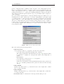
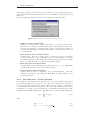
Chapter 3 deals with all menu entries of IDEA in the same structure as in the software’s menu bar. The functionality of all items is explained, sometimes with short
mathematical background. For further information, references to literature are included. Screen shots of dialog windows help to familiarize with the software.
For some main menu entries covering more complex features, a short overview is given
before each of the subordinated items are explained in detail.
Casually, references to other menu entries are not made by the number of the corresponding section in the manual, but directly by the name of this entry in IDEA’s
menu. It is then typed in italic fonts, with submenus separated by a textbar (’|’).
If a button is used in IDEA for shortcuts to a menu entry, it is shown at the left
margin aside the menu name.
In chapter 4, some evaluation procedures are worked out as a kind of tutorial for the
user.
1.5
1.5.1
What’s new in Version 1.5
New features
• Image- and Data Field windows now have scrollbars, which eliminates system
specific size restrictions related to the screen size. As a consequence, graph
8
1.5. WHAT’S NEW IN VERSION 1.5
windows for 1-dimensional data can also be scrolled. However, pictures in a
slide show are kept in full-size mode.
• A number of points can now be selected by a new draw feature (and by the
new polygon draw mode of course), and x,y and z values can be viewed and
saved in Info |Data at (Selected) Point(s), or even edited in Edit |Edit Data
at Selected Point(s). The main reason to add this, however, was to enable
unwrapping procedures to start from points in regions isolated from each other.
• The ability to draw polygons has been added, therefore there is the new feature Mask |Mask Polygon
• There is now the feature to make a ’One-Step’ phase unwrapping, subsuming
the scan for the 2π jumps and the unwrap itself.
• The famous branchcut phase unwrapping has been added, utilizing nearest
neighbour and minimum cost matching algorithms to minimize the overall
branchcut lengths.
• To test the quality of modulo 2π Data, the number of residues (inconsistences
where scanning unwrapping algorithms are likely to fail) can be determined
in Info |Number of Residues
• There is now an additional method to remove a linear phase shift, e.g. phase
plane, from unwrapped phase data. The plane to subtract can be determined
by planar regression of masked data, which reduces error influences from noise.
• For ASCII export, one can choose now between tabulator and space as delimiter
in File |Preferences.
• The ASCII output for invalid values (so far +NAN) can now be substituted by
a user-definable string in File |Preferences.
• The treatment of invalid data in the filtering process can now be defined for 2D
Data fields.
• Two filter routines for modulo 2π phase data have been added, both preserving
the ’sawtooth’ edges.
• In Edit |2D Data |Substitute Invalid Values, the possibilities to replace invalid
data by neighbourhood mean or median have been added.
• It is now possible to extract both interlaced fields from an Image.
• Image data can be squared.
• When applying Edit |1D Data |Rescale, invalid values are now substituted by
the spline routine. This way, be setting the scale factor to 1, one can interpolate
missing data.
• To remove linear tilt from 1D Data, one can choose now to fit a line through
data outside of the border lines.
• The feature File-Pool |Subtract Every ith File has been added. The files in a
File Pool can be divided in subgroups of definable size, and first or last file in
such a subgroup is subtracted from the other files.
• The counter of the files in File-Pool can be changed by adding a constant number.
9
1.5. WHAT’S NEW IN VERSION 1.5
• Three methods to determine phase data for phase-stepping speckle pattern interferometry have been included, which either require interferograms with subtraction fringes, or just one interferogram with altered object phase and four
phase shifted speckle pattern interferograms of the reference state of the object
(Phase Shift |Speckle ...).
• Spatial Phase Shifting algorithms for pixel-to-pixel phase differences of 120◦ and
90◦ have been included (Phase Shift |Spatial Phase Shifting ...).
• In the new version not only real- and imaginary part and amplitude can be
extracted from Fourier space, but also phase (2D-FFT |Show Phase ...)..
1.5.2
Amendments
• Subtraction of modulo 2π data fields resulted in a wrong sign. This has been
corrected.
• Adding a constant value to modulo 2π data fields includes re-mapping again to
the interval [−π, +π].
1.5.3
Known Issues
IDEA is widely, though not excessively tested. The latest operating system for development of the software has been Windows 2000, alternatively it has also been tested
with Windows 98 and Windows XP. Some problems have been noticed, which could
not be solved:
• At one Windows 98 system it has been observed that the startpoint of a line
and the corners of a polygon are not erased when a new drawing is started. This
did not occur at other PCs with the same operating system.
• On laptops, the fonts in dialogs might appear too small.
• Rarely, visualization of images or data fields are not actualized correctly and
appear white. With View |Refresh, the white picture can be repainted, but windows with this fault tend to inherit it to subsequently calculated data windows.
10
Chapter 2
Conventions and Definitions
Before we started to implement specific algorithms and procedures for processing
input data, we had to spend much brain work about organization and logistics of
all the data we would use for input and the data we would produce. The result of
these reflections are presented in this chapter. To understand the partially arbitrary
defined specific terms and the structure of data handling is essential for an effective
use of IDEA.
2.1
Definitions of IDEA-Specific Terms
As mentioned above, we are restricted to 256 colour pictures for all data visualizations.
To distinguish the data from the visualization itself, we defined specific terms. The
following specification shall give you an explanation of these terms, as this is the key
to understand this manual and the menu entries of IDEA.
2.1.1
Palette
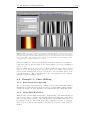
A Palette contains information of all 256 colours used for a visualization. It can also
be designated as a Look Up Table. In our case the information of one colour is given
by its red, green and blue portion (RGB-Code), each of it with a depth of 8 Bits. Each
pixel value refers to one of these Codes by giving the 8-bit ‘address’ (offset) within
the palette. IDEA provides several pre-defined palettes which can be applied to any
visualization. In these palettes, the 256th RGB-entry is reserved for the individual
mask colour (see below), whereas entry 255 is used for invalid values (see Sec. 2.3).
Entries 252 and 253 are used to show under- and overflow after remapping (also
explained below).
2.1.2
Picture
Following our definition, a picture is the visualization of any 2D-Data and Images.
The data itself is held in the background and is not affected by changing visualization
parameters. If you are interested not in the data itself, but in its visualization, you
can convert the data to a stand alone picture and save it as a uncompressed Windows
bitmap (*.bmp) with 256 colours. This picture cannot be distinguished from the
visual data representation. The essential difference is that there is no data in the
background anymore. Therefore, opening such a picture provides no usable data for
processing, unless it is converted to an Image (see below).
2.1.3
Image
In the context of IDEA, an Image is two dimensionally arranged data with a depth
of 8 Bits. Such an Image is by default represented by a gray scale Picture. Its
2.2. FILE TYPES AND FORMATS
palette consists of 252 gray scales from black (RGB 0 0 0) to white (RGB 255 255
255). Therefore, not all available gray levels are used, but this cannot be seen by the
human eye. Be aware that the Picture serves only as a visualization of the Image data
to be processed and to be saved. The remaining four palette entries are used for the
mask, underflow and overflow (see below). The visualization of the eight Bit data is
done line by line from top to bottom. If a bitmap is opened, its palette is checked for
non-gray entries. If such an entry is found, the bitmap is not accepted as an Image
and an error massage occurs. If not, the gray scale information is retrieved and then
visualized by a gray-scaled picture palette.
2.1.4
2D Data or Data Field
A Data Field is a two dimensionally arranged data in double precision format visualized by a picture. The 252 colour nuances correspond to the same number of
intervals between maximum and minimum of the Data Field. As by Images, the data
is visualized line by line from top to bottom.
2.1.5
Mask
The user can interactively mark data within Images or Data Fields. This can be
done by paint brushing using a mask colour, or by special algorithms masking certain
data values. Since masking is restricted to the visualization level, original data are not
harmed. The mask can be saved separately (see Sec. 2.2.8, Sec. 3.11.2 and Sec. 3.11.3).
In each palette, the 256th entry of the palette (offset 255) is reserved for the mask
colour.
2.1.6
Mapping
When an Image is opened, the data range from 0 to 255 refers to palette entries 0
to 251. So, for a Data Field the range between minimum value and maximum value
is divided into 252 intervals, each represented by one colour. ’Mapping’ is a term we
use for redefining the data range, for which the 252 palette entries are used. Values,
which are beyond the defined data range get the colour for overflow (offset 253), those
below are marked with the colour for underflow (offset 252). The modulo 2π data
is handled a little bit different. For visualization, values higher than π are always
regarded as overflow, values lower than −π as underflow.
2.2
File Types and Formats
The various implemented algorithms require input data of different types or origin.
For instance, the phase unwrapping methods are restricted to modulo 2π phase data.
The results of calculations must also be distinguished. To keep to the previous example, the result of phase unwrapping can only be phase data, whereas tomographically
reconstructed data may be of any type (e.g intensity).
To prevent any confusion, we decided to do a strict differentiation of all data types.
This allowed us to organize availability of menu entries in IDEA. Only those menu
entries are available, which can be applied to the data represented by the currently
active window. The others are grayed out. We hope you agree that the ease to obtain
a general view makes up for the somewhat pedantic differentiations. For those who
feel uncomfortable by these restrictions, IDEA allows to change the internal data type
(see Sec. 3.1.6 to Sec. 3.1.9) on one’s own responsibility.
2.2.1
File Type Classes
The various file types (or data types, respectively) can be separated into six classes.
You can find this classification also in the standard file selector dialog, where in the
12
2.2. FILE TYPES AND FORMATS
box entitled ’File Types’ you can select from different types distinguished by their
extensions. In the case of IDEA, you do actually not select a file type, but a class of
file types. These classes usually comprise files with different extensions. Here they
are listed up again, together with other unique file types which cannot be loaded or
saved with the standard file selector:
• Image: Two dimensional 8 bit data (binary or ASCII) regarded as gray scale
values. See Sec. 2.1.3 for further description.
• 2D-Data: Any two-dimensional data in double precision format, binary or
ASCII. See Sec. 2.1.4
• 1D-Data: Any one-dimensional data in double precision format, binary or
ASCII.
• Tomographic Input: File containing all input data for tomographic reconstruction. For detailed file structure see Tab. 2.2.
• File Pool: Collection of file names for collective processing.
• Graphic Format (Picture): Colour picture in standardized format. For our
interpretation of the term ’picture’ within the context of IDEA see Sec. 2.1.2.
• Filter File: 2D Filter kernel data. Can only be saved and loaded in Filtering
|User Kernel.
• Mask File: Contains location of masked pixels. Saving is only possible in
menu Mask |Save Mask, loading only in Mask |Add Mask File.
• Colour Palette File: RGB-Values for customized palette (ASCII). Loading is
possible only in Edit |Change Palette
• Angles: Contains angles of projections for tomographic reconstruction. Loading and Saving is only possible in Tomography |Edit Projection Angles
2.2.2
File Format Conventions
By default, IDEA saves data in the byte order used by the detected machine type
(result of detection shown at top of Protocol window). As most computers, PCs use
the little endian byte order, with the least significant byte of a word first. Avoid
porting data saved with such machines to big endian systems, which use reverse byte
order, and vice versa. It is clear that all data would be completely wrong interpreted.
To allow data exchange between different machine types, we provide a conversion
between little and big endian order. Refer to Sec. 3.1.11 for details.
The identification of most supported file formats is made by the first two bytes of
the opened file. We call these two bytes Identification Code (ID). It overrides the file
extension and is the same for data in binary and ASCII-format. In Tab. 2.3 the ID
is given for all file types.
2.2.3
Internal Format of Plain Image, 2D and 1D-Data
For Images, 2D-Data and 1D-Data we defined a most simple internal format. The
header of these classes consists of the ID and a information about the size of the
saved data field or data vector. For Images and 2D-Data the size information is given
by both width and height of the field. Here width is the number of data per line,
and height is the number of lines. The data is assumed to be stored line after line,
and this is also true for the visualization. Lines are shown from top to bottom in
the same order as they are read from file. The Frequency File is excepted from this
13
2.2. FILE TYPES AND FORMATS
simple concept. It includes complex spatial frequency data in the so called packed
order. See Sec. 2.2.4 for more information. For 1D-Data the size information consists
only of the number of data within the vector to read in. In all cases, data beyond the
given size is ignored. If less data is included than size parameters suggest, an error
message occurs and the file cannot be loaded.
The ID and size parameters are always in ASCII format, even for binary files, to avoid
possible allocation faults if the file should be opened at machines with wrong byte
order. The common header line structure for 2D-Data and Images is:
ID [width] [height] [format string for ASCII-files][new line]
For 1D data it is even more simple:
ID [number of elements] [format string] [new line]
Identification Code and size parameter(s) must be followed by a format string for
ASCII-files (see Sec. 2.2.12) in the same line. The data itself, whether ASCII or
binary, starts after a line feed. For example, the header of a phase field modulo 2π
with 256 rows, each row consisting of 512 data elements, is ’M2 512 256 %.6g’.
Apart from that internal formats, we support three external formats for saving and
loading Images. See Sec. 2.2.11 for further information.
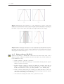
2.2.4
Internal Format of Frequency File
The Frequency File contains the complex amplitudes of the spatial frequencies of
an Image or 2D-Data field. The rather complicated structure of the data is due to
efficient coding of the Fourier transform for optimization of speed and minimization of
memory requirements. The resulting ’Packed Order’ of the data is standard and well
documented, e.g in [36]. Its structure is shown in Tab. 2.1. For ID, refer to Tab. 2.3.
The data for the horizontal Nyquist frequencies is delivered separately in a vector by
the algorithm. This data is splitted into parts of the same length as one line. Usually,
the last part has to be filled up to length of line with zeros. These additional lines
are appended to the packed field.
2.2.5
Internal Format of Tomographic Input File
This file type includes the one dimensional integral data of the different directions,
from which the reconstruction is calculated, and the corresponding angles of these
projections. See Tab. 2.2 for the structure of this file type and Tab. 2.3 for ID.
2.2.6
Internal Format of Filter File
This file type, which includes all data for a filter kernel, is completely in ASCII format
with following structure:
FL Width Height Multiplier Divisor [new line] Data
The common file-ID ’FL’ is followed by the dimensions ’width’ and ’height’ of the
kernel, which have to be both odd. ’Multiplier’ and ’Divisor’ define the constants D
and M in (Eq. (3.1)) used to normalize the results of convolution. They are followed
by the kernel elements in the next line, which are given row by row.
2.2.7
Internal Format of Colour Palette File
It is possible to import a custom Colour Palette to IDEA. Such a file has no header
line and consists of the RGB values line by line in ASCII format, each value smaller
than 256 and separated by a blank or comma from its neighbour. For example, to
import the gray scale palette, the file to load must have one of the following structures:
0 0 0 [new line] 1 1 1 [new line] . . . 255 255 255 or
14
2.2. FILE TYPES AND FORMATS
15
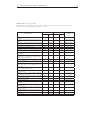
Table 2.1: Format of Frequency File;
Coordinates are given by the spatial frequencies f x in horizontal direction and f y in vertical
direction. The according number of periods in a Field of Nx pixels per row and Ny rows are also
shown. Indices min and max mean minimum and maximum of frequencies, with Nyquist frequencies
(nyq) regarded separately. Negative horizontal frequencies are the complex conjugate to the related
positive frequencies and are therefore redundant. For negative vertical frequencies, indices amax
and amin denote frequencies with maximum or minimum absolute value. The second part of the
table gives the vector with horizontal Nyquist frequencies, which are added as additional rows (last
row completed by filling up with zeros, if necessary). The complex amplitude is saved with its Real
(Re) and Imaginary (Im) parts, both in binary double precision format (8 bytes).
fx+
0
fx+
min
. . .
Periods
0
1
. . .
fy+
0
0
Re : Im
Re : Im
. . .
Re : Im
fy+
min
1
Re : Im
. . .
. . .
. . .
. . .
. . .
. . .
. . .
. . .
. . .
. . .
. . .
. . .
. . .
. . .
. . .
. . .
. . .
. . .
. . .
. . .
Frequency
. . .
Ny
2
fy+
max
−1
Ny
2
fy±
nyq
Ny
2
fy−
amax
−1
fx+
max
Nx
2
−1
. . .
. . .
. . .
. . .
. . .
. . .
fy−
amin
1
Re : Im
. . .
. . .
. . .
+
fy+
0
fy+
min
. . .
Periods
0
1
. . .
Nx
2
Re : Im
Re : Im
. . .
Frequency
fx±
nyq
fy+
max
Ny
2
−1
. . .
fy±
nyq
Ny
2
. . .
fy−
amax
. . .
fy−
amin
Ny
2
. . .
1
. . .
Re : Im
−1
. . .
Table 2.2: Format of Tomographic Input File;
The effective length is the length of the shortest projection included and is used by the reconstruction
algorithms. From longer distributions, data out of range at the sides is ignored (center is always
fixed).
Location/Repeats
1. line
2. line
n lines
n times
Data
Identification Code
Effective length of projections
Number of Projections (n)
Comment (max. 1024 byte read)
Relative pathname of source projection file
Projection angle [new line]
Length of projection [new line]
Projection Data
Format
ASCII
ASCII
ASCII
ASCII
ASCII
binary
2.2. FILE TYPES AND FORMATS
0,0,0 [new line] 1,1,1 [new line] . . . 255,255,255
2.2.8
Internal Format of Mask File
Completely in binary format, this file type includes information about the location
of masked pixels (or data, respectively) of a master picture. To save disk space, we
decided to set one mask-bit for every pixel of the master picture. If the pixel is
masked, the bit is set to 1, else to 0. The bits are packed together in groups of eight
to form bytes, which is the data format used to save a mask. For saving, the master
picture is scanned row by row for mask colour, setting the bits in the corresponding
bytes. At the end of the file, some lower significant bits in the last byte are not set if
the number of pixels in the master picture cannot be divided by eight. This surplus
on bits keeps its initial values of zero, which has no effect since they are never referred
to.
The masked data is internally treated as a vector, so the size parameter has to represent the length in bytes. The size check made before adding a mask to a picture is
therefore limited. For instance, the mask of a 256 × 512 Image fits well on an Image
with size of 1024 × 128. No error message would appear in this case.
2.2.9
Internal Format of File Pool File
The File Pool is in principle a collection of file names. All data is in ASCII Format
and in the following order:
PO pathstyle [new line] paths (separated by line feeds)
The common file-ID ’PO’ is followed by the pathstyle-parameter which can be either
’relative’ or ’absolute’. A relative pathstyle means that the filenames are given relative
to the location of the File Pool. In case of the ’absolute’ style the full paths are
required. The character for the folder separator can be either a backslash ’\’ or a
slash ’/’. Both are accepted and converted to the appropriate style of the operating
system in use.
2.2.10
Internal Format of Projection Angle File
This file contains raw ASCII-data without header and ID. The projection angles must
be separated by a line separator or by an empty space.
2.2.11
External Graphic Formats
In addition to the self-defined plain file formats we support three external formats:
Bitmap (*.bmp), X Pixmap (*.xpm) and the not so common Imaging Technology
Itex format (*.pic, not to be confused with the better known PC Paint and Lotus
PIC format with same extension). The Itex format has true eight bit binary pixel
data giving directly the gray scales. It differs from our own Image format (*.img) only
by its longer header (offset to image data 64 byte, offset to width 4 bytes, offset to
height 6 bytes). On the contrary, the Bitmaps include a palette of 256 RGB-encoded
colours (see Sec. 2.1.1). For the format of Bitmap, see [29]. The X Pixmap has an
unlimited colour palette and must be converted to an IDEA-picture for further use.
A detailed description of the X Pixmap format may be found in [20].
When opening a file with one of these formats, the palette is checked. If all entries are
gray-scales and are not more than 256, the file is automatically identified and opened
as an Image. Otherwise, if at least one entry is not gray-scale, the file is identified as
a Picture (see Sec. 2.1.2).
16
2.3. HANDLING OF FLOATING POINT EXCEPTIONS
2.2.12
Saving ASCII data
Any of the internal data can be saved in ASCII format. Especially for 2D-Data, a
decision must be made about the number of relevant digits. To offer the user as much
flexibility as possible, IDEA accepts format strings equal to those used for all printf()commands of ANSI C (a detailed description of this format string can be found in
various C/C++ references, e.g. in [23]). For example, to get float data with 6 relevant
digits, write ’%.6g’, which is the default string. For scientific notation and 8 digits,
you have to enter ’%.8E’. These are simple examples, but the format string of C offers
you much more possibilities like adding signs, preceding zeros, forcing decimal etc.
But be aware that the format string is not checked by IDEA. Incorrect inputs will
likely result in corrupted ASCII-entries!
2.3
Handling of floating point exceptions
Depending on the settings made by the operating system, the floating point unit
(FPU) raises exceptions for specific operations according to IEEE-floating point specification. For instance, Windows95/NT initializes the FPU to raise an exception for
division zero by zero, which terminates the running program, although the result of
this operation is a specific encoded symbol ’NaN’ (not a number). To override such
settings, IDEA re-programs the FPU at startup to be less rigid. In fact, all exceptions
are deactivated. Results of mathematically non-defined values are represented by the
already mentioned symbol NaN, results of infinity (e.g. 1/0) are referred to as ’+Inf’
or ’-Inf’.
With the FPU-settings used for IDEA (other software in use is not concerned), it is
possible to perform any operation on data including NaNs and Infs. The results are
well defined and of course again non-values.
When data including such non-values is saved in ASCII-format, the symbols are written as +NAN, -NAN, +INF or -INF (if sign is printed depends on compiler used for
actual version of IDEA). In binary data, they are encoded in IEEE-standard binary
format.
Exchanging such data with other software could lead to serious problems. Therefore
we implemented routines to substitute the symbols by (valid) user defined values
(Edit |2D-Data |Substitute Invalid Values).
Not all algorithms, especially those for reconstruction, are able to tread invalid values
which may lead to corrupted results if they are applied to Data Fields containing
NANs or INFS. Such data need to be ‘cleaned’. For 2D-Data Fields, this can be
achieved for example by substituting invalid values and subsequent filtering.
To show the location of non-values in data window, we use a reserved colour with
offset 254 (entry number 255) in the palette of the representing picture. It is similar
to the mask colour, but with reduced luminance.
2.4
Input Macros and Operators
In all text boxes for values input, macros can be used (see Tab. 2.4). Be aware that
use of ‘min’ and ‘max’ are restricted to dialogs which are directly connected to Images,
2D- or 1D-Data fields.
Additionally, for all value inputs the operators for division (‘/’) and multiplication
(‘*’) can be used. Macros and operators can be used simultaneously. For the macro
‘pi’, a preceding factor without an operator is treated as if multiplication would be in
parenthesis (e.g. 1/2pi = 1/(2π), whereas 1/2*pi = 1/2 · π).
17
2.4. INPUT MACROS AND OPERATORS
18
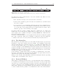
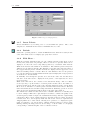
Table 2.3: File Types of IDEA;
Extension is the default file extension, ID is Identification Code in the file header, Class is the
Format Class defined in IDEA (see list in Sec. 2.2.1).
Extension
Description
Image - Plain 8-bit Image Data (internal
format)
Bitmap - Standard Windows Graphics Format
Pixmap - Standard X Window Graphics
Format
Format of Imaging Techn. ITEX software
Interferometrical Phase Data
Interferometrical Phase Data modulo 2π
Frequency Data - Complex Result from
2D-Fast Fourier Transform
Data reconstructed by Tomographical Algorithm
Projection - 1D integral data used together
with other projections to perform tomographical reconstruction
1D integral data to be Abel-inverted
Abel-reconstruction - 1D data reconstructed by Abel-Inversion
Tomographic Input - File containing all
data necessary for tomographical reconstruction
File Pool - Collection of filenames to perform collective processions
Image in raw ASCII format without header
(export only)
1D-Data in raw data format without
header (export only)
2D-Data in raw data format without
header (export only)
General 1D-Data
General 2D-Data
File containing data for user defined filter
kernels
Mask File - contains info about location of
masked data
Colour Palette File - list of RGB values
(input only)
Multiline Window - Collection of 1D-Data
distributions (export only)
Angles - Projection Angles
Preferences
ID
Class
binary
ASCII
binary
ASCII
.img
.dat
ig
IG
Image
.bmp
-
BM
-
Image/Picture
-
.xpm
-
/*
Image/Picture
.pic
.pha
.m2p
.frq
.dat
.dat
.dat
IM
ph
m2
fr
PH
M2
FR
Image
2D-Data
2D-Data
2D-Data
.tor
.dat
tr
TR
2D-Data
.pjn
.dat
pj
PJ
1D-Data
.abl
.abr
.dat
.dat
ab
ar
AB
AR
1D-Data
1D-Data
.tom
-
to
-
Tom. Input
-
.fpl
-
PO
File Pool
.bim
.aim
-
-
Image
.b1d
.a1d
-
-
1D-Data
.b2d
.a2d
-
-
2D-Data
.bin
.bin
-
.flt
1D
2D
-
FL
1D-Data
2D-Data
Filter File
.msk
-
ms
-
Mask File
-
.pal
-
-
-
-
.asc
-
-
-
-
.asc
.cfg
-
-
-
2.5. THE GRAPHICAL USER INTERFACE OF IDEA
19
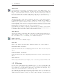
Table 2.4: Input Macros;
In dialogs of IDEA, macros can be defined in text boxes instead of values. The input is scanned
non-case sensitive for these macros.
2.5
Macro
Interpretation
nan
invalid
+inf
-inf
min
max
pi
-pi
‘Not a number’ (see Sec. 2.3)
Same as nan
‘positive Infinity’ (see Sec. 2.3)
‘negative Infinity’ (see Sec. 2.3)
Minimum of related Image, 2D- or 1D-Data
Maximum of related Image, 2D- or 1D-Data
Constant π
Constant −π
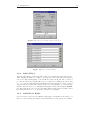
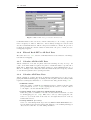
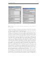
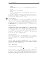
The Graphical User Interface of IDEA
If Windows 95/98/NT is used, all opened or created data fields are visualized in child
windows managed by IDEA’s main window. You have always access to the Menu Bar
on the top of the main window, where all entries are grayed out which are not allowed
for active child window data.
X Window does not allow this hierarchy. Each child window has to have its own
Menu bar with allowed entries.
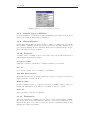
The Status Bar at the bottom of the Main Window (or Child Window, in case you use
the X Window Version) is designed to give the user as much information as possible
about the active window and the current interaction. In addition, we added an
automatically updating protocol window to help you keeping track of your evaluation
steps. Both elements are described in this chapter.
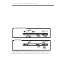
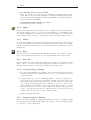
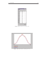
The basic kind of interaction with data windows is the selection of specific data. We
provide the possibility to select areas, investigate pixel data, extract line data and
even to paint within a picture without destroying the pixel information behind the
colour (see mask, Sec. 2.1.5). You will find further information about these features
in this chapter.
2.5.1
Data Selection in Active Window
Paint Mask
To mark Image data or 2D-data, for example to exclude it from calculations or to
set it to specific data, use the right mouse button, hold it down and draw within the
window. At every detected position of the mouse pointer a square or circle is drawn
in mask colour. Size and shape of these mask elements depend on the actual settings
of mask pen width and mask pen style. The data represented by the active picture is
not affected by the mask, which can be saved in an own mask file.
Draw Line
After switching to Line Draw Mode (global switch, see Sec. 3.3.10), one can select the
data behind pixels on a line, which can be drawn into the active Image or 2D-data
window. To do that, choose a starting point, press the left mouse button to start
drawing and move on to the desired endpoint. By pressing the left mouse button
again, you select the end point of your line. If CTRL key is held after starting the
line, drawing is restricted to vertical and horizontal lines. Refer to Status Bar (see
Sec. 2.5.2) for feedback about coordinates.
The position of line pixels are calculated from starting point and endpoint coordinates using the Bresenham algorithm [12]. Be aware that data is NOT automatically
arranged from left to right, but in the direction in which the line was drawn!
2.5. THE GRAPHICAL USER INTERFACE OF IDEA
Draw Rectangle
For choosing an area within a picture, one has to switch to Rectangle Draw Mode
(global switch, see Sec. 3.3.11). The selection can be done in the same way as you
would draw a diagonal line in Line Draw Mode. The selected area includes the drawn
border lines. As modification keys, the CTRL key allows to draw squares and the
SHIFT key allows only rectangles of size 2a × 2b ( a and b positive natural numbers).
Hold down these keys after setting the start point. Refer to Status Bar (see Sec. 2.5.2)
for feedback about coordinates.
Draw Crosshairs
In Crosshairs mode (global switch, see Sec. 3.3.12), the pixel at the intersection of a
vertical and horizontal line crossing the whole picture is selected by left mouse click.
The crosshairs can be moved by holding down the left mouse button. To select current
pixel, release mouse button. As for other draw modes, coordinates are simultaneously
presented in the status bar.
Draw Polygon
In Polygon mode (global switch, see Sec. 3.3.13), a left mouse click selects a corner
pixel of a polygon. The last selection can be cancelled by pressing the right mouse
button. When all corners have been selected, quit the process by a left button double
click into the 2D Data field or Image. At the position of the double click, the x-shaped
start pixel for the mask fill is set, which is the last entry in the related coordinate list.
Take this into account when drawing polygons by values (see Sec. 3.3.15). The start
pixel can be reset independently from the drawn polygon by pressing the left mouse
button when the Control key (Ctrl) is held. The new position of the start pixel is
then set at the mouse cursor position. A mask filled into the polygon does not cover
the polygon border lines.
Select Multiple Points
In this draw mode (global switch, see Sec. 3.3.14), a left mouse click selects a pixel
by marking it with a ’x’. The whole selection can be reset by pressing the left mouse
button when the Control key (Ctrl) is held. The first point of the new selection is
then set at the position of the mouse pointer. Note that the left mouse click function
overrides the draw mask function. Therefore, when a mask should be drawn in the
Image or 2D Data field, one has first to change the draw mode. There is another
distinctness of this draw mode: When copying a multi-point selection into a window
(see Sec. 3.3.16), then the actual point selection is not overwritten, but expanded by
the points in the other window.
Select Borders and Center of 1D-Data
For Tomography and Abel Inversion, borders and position of center must be defined
within a graph showing integral data. The borders are represented by blue vertical
lines through the graph, initially located at the left and right side of the graph. These
lines can be positioned either by mouse action or by typing coordinates into text fields.
For integral 1D-Data mentioned above, you can move the blue border lines with
mouse. If you point the mouse cursor to such a line, it changes its shape to a horizontal
arrow. By pressing and holding down the left mouse button, the borderlines can be
moved within the graph, keeping symmetrical position relative to the center line.
For Abel 1D-Data, holding down the right mouse button ’unlocks’ the borderlines
from the center and each of it can be shifted independently.
Likewise, the red center line can be moved with the mouse. The left mouse button
shifts the center together with the border lines. Again, Abel 1D-Data uses also
20
2.5. THE GRAPHICAL USER INTERFACE OF IDEA
Figure 2.1: Basic structure of Status Bar;
1 Menu Section, 2 Coordinate Section, 3 Draw Mode Section, 4 Mouse Pointer Section.
the right mouse button, which allows to move the centerline only. There are some
restrictions of movements:
• The centerline can only be moved between the border lines.
• Center- and borderlines together can only be moved until one border line reaches
the border of graph.
• If border lines are moved simultaneously (left button), but are asymmetrical to
the center, the opposite border jumps to symmetrical position when you click
on a border line. In case this position is not valid, mouse move has no effect
until the opposite border is in range of the graph.
To position a line at a certain coordinate, write the coordinate into one of three text
fields at the bottom of the window, marked with ’L’ for left border, ’C’ for center and
’R’ for right border. Confirm your input by pressing ENTER key. This shows the
line at the specified location.
Contrary to integral 1D-Data for tomography and Abel inversion, simple line graphs
have only a center line. There is no possibility to define its location by typing the
coordinate, but it can be moved by mouse in the same way as described above.
2.5.2
The Status Bar
The Status Bar of the main window (or active window in X) is used to give the user
information of the active window and some settings. Its organization varies with
data type and with mode of interaction (see Sec. 2.5.1). The bar is divided into four
sections. Corresponding to Fig. 2.1, we enumerate them from left to right. In section
1, a short description of the highlighted menu entry is shown. If the platform in use
is Windows 95/NT, the help text of entries opening a submenu is not correctly shown
in IDEA. In fact, you see help text of the previous valid entry instead. Sorry for that,
but this is not within our responsibility.
Section 2 shows coordinate data of a line, a rectangle or crosshairs used to select data.
In section 3, information about used draw- and mask-mode is given, whereas section
4 shows mouse position and data value located there.
In Fig. 2.2, the contents of the Status Bar for 2D-Data and Images is shown, depending
on Draw Mode. For 1D-Data, refer to Fig. 2.3.
2.5.3
Protocol Window
After startup, a child window titled ’Protocol’ is automatically created. At this time,
it contains some information about pre-checks. From then on, all your important
actions are protocolled in this window as short text lines. Most important, every
creation of data is reported, including information about the automatically created
window title. If write protection is disabled, the user is allowed to add personal notes
or delete contents. It is not possible to close this window, but it can be made invisible.
21
2.5. THE GRAPHICAL USER INTERFACE OF IDEA
Figure 2.2: Contents of Status Bar for Images and 2D-Data;
Contents of Coordinate Section (see Fig. 2.1) depend on active draw mode. Identical contents are
omitted. For pure Pictures, there are no mask entries in Draw Mode Section. For the Step Function
data type, which is saved as a Picture, the Status Bar is quite different from standard configuration
and therefore shown separately.
22
2.5. THE GRAPHICAL USER INTERFACE OF IDEA
Figure 2.3: Contents of Status Bar for 1D-Data
Note the difference in Mouse Pointer Section: For Multiline Graph, the right value gives the yposition of the active mouse pointer in the graph plane and is not related to any plotted curve. For
the standard 1D-Graph, the y-value on the curve at x-position of the mouse pointer is shown.
23
Chapter 3
IDEA Menu Entries
In this chapter the functions of all menu entries are explained in the same hierarchy
as they appear in IDEA. Descriptions of all dialog windows and input parameters are
included.
In the text, references to menu entries are written in the same style as paths, but
with vertical separation and emphasizing. For example the submenu ’Save As ...’ of
the main menu entry ’File’ is referred to as File |Save As ....
To avoid repeating descriptions, some consecutive menu entries are comprised if differences are marginal. In many cases actions are restricted to the ’Active Window, a
term we use for this window which is currently in the foreground, either after creation,
after a mouse-click on the window, or after selection in the main-menu entry Window
(not for X-Window System). It is marked by a different colour of the window’s title
bar.
3.1
File
This main-menu entry deals with all basic kinds of file- and file-type handling, creation
of empty data structures and with preferences of IDEA.
3.1.1
New ...
File Pool, Tomographic Input File, Slide Show, Multiline Graph
Here, an empty window dedicated to the corresponding data type can be created,
which can be filled up with file data or data already available on the IDEA-desktop.
1D Integral Data, Abel Reconstruction
Since it is possible to paste 1D-Data from the clipboard (Windows 95/NT only),
empty 1D-Data windows (graphs) can be created to be filled up with data from the
clipboard by Edit |Paste. Of course, values can also be typed in directly. By default,
the new 1D-Data are initialized with zeroes.
As input parameter, you have to define the number of data you want to include in
your graph.
Scale Bar
A Scale Bar is a picture with size of 128 × 256. From the lowest line of the picture up
to the top the colours of the actual palette from 0 to 255 are used (including mask,
over- and underflow colours, if they exist). By default, the grey scale picture palette
is used. This bar may serve as colour reference for a scale added to a pseudo-colour
visualization of any data. Resizing is possible using Edit |Rescale Image/Picture.
3.1. FILE
25
Simulated Interferogram
This creates a simulated interferogram with optional noise added. Several parameters
must be specified in the dialog shown in Fig. 3.1.
Figure 3.1: Dialog for Creating New Simulated Interferogram
• Number of fringes
For circular fringes, the number refers to number of fringes in the diagonal of
the interferogram to be created.
• Width of Interferogram
• Height of Interferogram
• Minimum Intensity Imin [0-254]
Defines minimum intensity of ideal cosine distribution (without noise).
• Maximum Intensity Imax (Imin-255]
Defines maximum intensity of ideal cosine distribution (without noise). Must
be greater than Imin.
• Phase Shift
Phase shift in degrees. By default, phase is 0 at center for circular fringes, at
left side for vertical fringes and at upper side for horizontal fringes.
• Noise Density (0-1]
A random number generator creates a noise density value between 0+ε and 1
for every pixel. If this value is below the defined Noise Density, noise is added
for this pixel. Entering of 1 causes noise in every pixel, defining 0.5 means that
to 50% (statistically) of all pixels noise is added.
• (Relative/Absolute) Noise Amplitude
Defines range of noise Amplitude. The value of noise, which is added to the
pixels of the ideal interferogram (those which passed density test, see above) is
generated by a random number generator. It is statistically distributed between
(- noise amplitude) and (+ noise amplitude). The sum representing new pixel
value may be out of range (0-255), so overflows are set to 255, underflows to
0. The amplitude can be given absolute or relative (see below). Define 0 for
amplitude if you do not want to have noise added.
3.1. FILE
• Use Absolute Noise Level (to check)
If the box is active, the value for Noise Amplitude is interpreted as absolute
value. Else, the absolute noise amplitude for each pixel is calculated from pixelvalue×relative Noise Amplitude. In this case, minimums of a interferogram have
less noise than the maximums.
• Vertical/Horizontal/Circular (to select)
Determines appearance of fringes.
3.1.2
Open ...
Read file from disk using the standard file selector of Windows 95/NT or X Window.
Select desired file type (see Sec. 2.2.1) to be viewed in file list or, for X-Window, from
the submenu. IDEA accepts only files with correct ID (see Tab. 2.3). Consider byte
order settings in File |Preferences |Open File Assuming Little Endian Byte Order.
3.1.3
Close ...
Close the actual Window. If the data represented by the actual window were changed
or created by calculation, the user is asked if this data should be saved before closing.
On the other hand, if data just were read from file and never changed, it is closed
immediately.
3.1.4
Save
Save data in current format with the filename in the title bar of the window. Consider
byte order settings in File |Preferences |Save File with Little Endian Byte Order.
3.1.5
Save As ...
Select new name and format in the standard file selector dialog of the platform in use.
Refer to Tab. 2.3 for more details about suggested extensions. Consider byte order
settings in File |Preferences |Save File with Little Endian Byte Order.
3.1.6
Convert/Copy to Image
1. To convert a 2D-Data Field to an Image, the field’s data is subdivided into 256
intervals. All pixel values within interval i (i = 0, 1, ..., 255) are then converted
to the 8-bit value i.
2. If a pure picture (e.g. 256 colour Bitmap) shall be converted to an Image, one
has to define how the gray level I should be calculated from the 8 bit colour
information R (red), G (green) and B (blue) in a dialog window. In literature
(e.g. [29]) the following expression is recommend: I = (77 · R + 151 · G + 28 ·
B)/256. This is the ’Standard’ option in the dialog shown in Fig. 3.2. Apart
from that you can select, ’Red’, ’Green’, ’Blue’ and ’Custom’. The three text
boxes to the right show the factors of R,G and B for the chosen option. If
’Custom’ is selected, the factors can be defined by user.
3. Images are simply duplicated.
3.1.7
Convert/Copy to Picture
This converts the visualization of Images and 2D-Data to a 256 colour-Bitmap, using
the current palette (including mask-, under- and overflow colours, if existing). Apply
to a Picture to create a duplication.
26
3.1. FILE
27
Figure 3.2: Dialog for Converting Picture To Image
3.1.8
Convert/Copy to 2D-Data
Converts an Image to a Data Field by just expanding the gray values (8 bit) to floats
with double precision. Data fields are duplicated.
3.1.9
Change Filetype ...
For 1D-Data and 2D-Data we allow the user to change to a different file type within
these classes to eliminate any file type specific restrictions. Be aware, this is done by
your own responsibility. Don’t be surprised when a 2D-reconstruction from tomography looks weird as a modulo 2π Field.
3.1.10
Protocol ...
Contents of Protocol Window can be saved and loaded only in this menu and not
with standard Open and Save entries.
Load Protocol File
Substitute contents of current Protocol Window with Protocol from file.
Save As ...
Save current contents of Protocol Window to ASCII-file.
User Edit Mode Disabled
This menu entry is active by default. In this case, the Protocol is protected from user
input. Uncheck to activate edit mode.
Window Visible
If active (default), the Protocol Window is present on IDEA’s desktop. Else it is
hidden, but still existent. Note: The Protocol Window cannot be closed!
Clear All
Delete all entries of the Protocol Window.
3.1.11
Preferences
Here some preferences for IDEA can be set, saved or loaded. After startup of IDEA,
the current directory and, afterwards, the directory of idea.exe is searched for a configuration file. If no *.cfg could be found, the options for maximum safety in data
handling are activated by default.
3.1. FILE
Set Working Folder
By default, any window title includes the path of the file relative to the folder from
which IDEA has been started. For the elements in a File Pool, the path is given
relative to the location of the File Pool file. For both cases, the ‘master’-folder can
be redefined to a common ‘working’- folder with this menu entry. All window titles
are actualized afterwards.
Image/2D-Data/1D-Data: Create New Window
If this menu item is active, for every edit- and filter-operation on data of chosen type a
new window is created (default). If you like experimenting, but not piling windows on
your desktop, deactivate the switch. Creation of new Images is then only done if two
different data sets are used to create a new one (eg. Edit |Subtract Image/2D-Data
or Edit |Insert Image/Picture/2D-Data, apart from any Mask-operations.
File Pool - Automatically Update
If you have large File Pools or a slow machine, deactivate this switch. Otherwise,
contents of File Pools are constantly updated. Files not existing any more are then
automatically removed from the list (works only for Windows95/98/NT-version).
Zoom Window - Automatically Update
Activating this menu item causes zoom windows (see 3.4.1) to retrieve possibly
changed master window information on activation (Windows 95/98/NT only).
Image/2D-Data - Enable Operations in Selected Area
To restrict edit- and filter-operations to an area selected by drawn rectangle, activate
this menu item (Resize- and Rescale-Commands excluded). You will be asked every
time if you want to perform the operation on the whole data set or only on the selected
area. After some time this may become annoying, therefore the option is deactivated
by default.
Mask - Enable Operations in Selected Area
To restrict mask-operations to selected area (rectangle drawn in window), activate
this menu item. You will be asked every time if you want to perform the operation
on the whole data set or only on the selected area. After some time this may become
annoying, therefore the option is deactivated by default. Be aware, mirroring and
symmetrizing cannot be restricted to selected area.
Abel Inversion - Strict Symmetry Checking
To be on the save side for Abel calculations, this menu item should be activated
(default). In this case, before inversion is performed all integral 1D-Data (*.abl) are
checked for symmetry with axis at centerline and data outside of left border line is
ignored.
Otherwise, only data between left border line and center line is taken into account
for calculation. Symmetry is just assumed.
Open File Assuming Little Endian Byte Order
With this menu item activated (default on PCs), the files to open are assumed to
have little endian byte order (eg. files created at PCs). Deactivate it if you want to
open files with big endian byte order. If you are not sure which byte order is used by
28
3.1. FILE
your machine, look at the pre-check entries in the first lines of the protocol window
(see 2.5.3).
Save File with Little Endian Byte Order
With this menu item activated (default on PCs), files are saved with little endian byte
order. Otherwise, big endian byte order is used. As long as this switch is in the same
state as the one in the previous menu item, you will not have any problems, at least as
long as you do not export data to other machines. Obviously, to have different states
is very dangerous. For exporting files with different byte order, it is recommended to
convert all files using a File Pool.
Substitute Invalid Data for Raw ASCII Export
The string representing invalid data in ASCII files created by exporting data in the raw
ASCII format (e. g. without header, see Tab. 2.3) is substituted by the string defined
in the dialog box. This has been included since invalid data is the most critical issue
when importing data with third party software. If the software you want to import
data to does not accept invalids at all, you have to preliminary substitute them within
idea (Edit |2D Data |Substitute Invalid Values, the same for Edit |1D Data).
Set Tabulator as Delimiter for ASCII Export
By default, data is exported in ASCII format using separating spaces (blanks) between
numbers. Here one can replace the blanks by tabulators. This is another feature added
for the sake of compatibility with other software. Other than the substitution of the
string for invalid data, this is not restricted to export in raw ASCII format, since
IDEA is capable of reading data with tabulator delimiters.
Load Preferences
Load a previously created Preferences-file (*.cfg), an optional ASCII-File containing
all information about the settings in the Preferences menu to be actualized after
loading. During startup, idea.cfg is searched, first in the current working folder, then
in the folder where idea.exe is located. The searching and finding-process is reported
in the protocol-window. Note: the file in the current folder overrides any configuration
file in the directory of idea.exe.
Save Preferences
During startup, the optional file idea.cfg is searched, first in the current working
folder, then in the folder where idea.exe is located. The searching and finding-process
is reported in the protocol-window. All preferences settings are made according to
the ASCII-contents of this file. After changing these settings, it is possible to save
the new preferences in a file with the same structure as idea.cfg, using the standard
file selector. Overwriting of idea.cfg will redefine the startup-settings.
Set Default Preferences
Ignores any settings of preferences read from file, and uses IDEA’s internal default
settings for maximal safety in data handling during work.
Set Preferences for Fast Works
Ignores any settings of preferences read from file, and uses IDEA’s internal alternative
settings for maximal data-handling speed during work.
29
3.2. FILE POOL
3.1.12
Exit
Finish your work with IDEA and leave the program.
3.2
File Pool
Life would be easy if all problems could be solved by only one image acquisition
and its evaluation. In reality, one has to bother with multi-directional or temporally
resolved measurements, to mention just a few experimental requirements which leads
to a large amount of image data.
Having spent hours applying the same evaluation step again and again on dozens of
images or data fields, we decided to avoid such a work with IDEA.
The solution we are able to present is the File Pool. The idea was to allow the user to
collect files in a ’pool’ and to apply most of the algorithms used for phase evaluation,
editing, filtering and reconstructing to all collected files. The File-Pool itself includes
just the filenames of the collected files, not the data (see Sec. 2.2.9). You are not
restricted to only one filetype within a File Pool. Feel free to comprise all files related
to the same project. For file-type specific operations it is possible to extract all files
of appropriate type from the main File Pool into a new one. This way you can easily
overlook your work and save much time.
The operation performed on a File Pool is repeated file after file, and the results are
saved after completion of each step. Structure of filenames and the format of saved
data can be defined by the user. All created filenames are collected in a new File
Pool.
To create a empty File Pool, use File |New |File Pool (see Sec. 3.1.1). By doubleclicking a file name in the File Pool Window, you can open it in a separate window.
Whenever an operation is applied to a File Pool, a dialog titled Saving Options for
File Pool pops up before the calculations start (see Fig. 3.3). In this dialog you can
define a ‘Saving mode’ in the upper left hand corner. In general, you have the choice
between overwriting the files in the File Pool with the results (‘Overwrite existing
files’) or to save the results with new filenames (‘Save as new file’).
New files require new filenames. A part of this is overtaken from the filenames in the
source File Pool (name). A second part (*) has to be defined by the user in the left
text box at the bottom of the dialog. At the upper right hand corner you can choose
between setting the user defined part in front or behind the overtaken one.
You can choose between general binary or ASCII format or corresponding Raw data
without Identification Code (see Tab. 2.3). In general, you also have the ’Same format’
option, which saves results in the same format as the source files. For image data,
the section to the right is available, where you have to define the desired file type
for binary Images. If ‘ASCII-Data’ or ‘Raw-ASCII’ was selected as Saving Format,
the ‘ASCII Format String’ must be defined in the lower right of the window (see
Sec. 2.2.12).
3.2.1
Add File(s)
Add files from disk to File Pool by using the standard file selector of the platform in
use, for which Multi-File-Selection is activated. In Windows 95/NT, use the SHIFTor CTRL key in conjunction with the left mouse button to choose a group of files in
the list of filenames. In X Window Systems, you can specify a wildcard.
Note: The last selected filename appears always at the beginning of the text line
showing the current selection (located below the filenames-list), reversing the temporal
order of your selection. Be aware that the number of selected filenames is limited since
the buffer for the corresponding characters is restricted by the Windows operating
system. Without warning message, all filenames which did not find place in this buffer
are simply ignored.
30
3.2. FILE POOL
31
Figure 3.3: Dialog to set Saving Options for File Pools
Figure 3.4: Dialog for ‘Add n File(s)’
3.2.2
Add n File(s)
Add a specific number of files from disk to File Pool by using an adapted file selector.
After defining the number n of files to open, the file selector window appears with n
text boxes. Type in full paths, or use the Browse button at the left side of each box
to select the file by the standard file selector. Compared to multiple file selection in
Sec. 3.2.1, you can easily handle files in different folders. In addition to that, we added
a special feature for files with counters at the end of the filename, eg. image23.bmp.
Put the cursor in a text box containing the full path of such a file and press ENTERkey. The subsequent text boxes are then filled with the same path, but with counter
incremented from box to box. Previous contents are overwritten.
3.2.3
Add Files in Folder
Select a folder (or directory for X Window Systems) to add all files located there to a
File Pool. Don’t change the character in the filename-box as it is used as a dummy.
3.2. FILE POOL
3.2.4
Remove Marked File(s)
Entries marked by mouse selection (for multiple selection use left mouse button in
conjunction with SHIFT or CTRL key) are removed from the File Pool.
3.2.5
Clear All
Remove all contents of the File Pool. Remember, this does not delete the files from
disk as in Sec. 3.2.6, since a File Pool only contains paths.
3.2.6
Delete (Marked) Files From Disk
All files collected in a File Pool are deleted from the harddrive. This way, unwanted
results of File Pool operations are easily removed without switching to other applications and redoing the file selections for deletion.
3.2.7
Open Marked File(s)
Entries marked by mouse selection (for multiple selection use left mouse button in
conjunction with SHIFT or CTRL key) are opened and corresponding windows appear.
3.2.8
Sort Alphabetically
Use this to sort the filenames in a File Pool alphabetically. The entries are accordingly
reordered.
3.2.9
Extract Every ith File
Creates a new File Pool including every ith file from the actual File Pool. In the small
dialog one has only to define the value i. For example, after an acquisition of 250
interferograms for temporally resolved measurement, it’s a good idea to start with
the evaluation of a few representative images to see if everything worked out well. So
after creating a File Pool with all 250 images, it is possible to evaluate only 10 images
by choosing i = 25 in the dialog of this menu entry without selecting the according
filenames by hand.
3.2.10
Extract (Marked) Files
Creates a new File Pool with all marked entries. If nothing is marked, the File Pool
is duplicated.
3.2.11
Extract (Marked) Images/2D-Data/...
It is not possible to perform file-type specific operations on File Pools including files
of different types. To solve this problem, we made it possible to create new ’pure’
File Pools by copying all entries of the selected type from the superior File Pool. If
some entries are marked, only those are taken into account.
This allows a convenient file organization, especially for files spread around different
folders. Collect all files of a project in a main File Pool and create all possible ’pure’
subordinates. Perform evaluations on these File Pools. At the end of the session,
merge all relevant results into the main File Pool. This keeps your project files
together and allows direct access all the time.
32
3.3. EDIT
3.2.12
Subtract Every ith File
In the upcoming dialog, one has to define the ’Subtraction Group Size (i)’. Starting
from the top, all filenames are then divided into subgroups, each of it containing i
filenames. Remaining names are ignored. The selection in the dialog checkbox sets
either the leading file or the last file represented in a subgroup as the argument of the
subtraction. This file is then subtracted from the other i − 1 files in the group. A new
File Pool is then created containing the filenames of the files created as results of all
subtractions. This In-FilePool-Subtraction has been designed for series recordings of
sets of phase stepped Speckle interferograms, each followed by one interferogram with
altered object state. This File Pool operations allows to create a series of subtraction
fringes interferograms (also referred to as secondary Speckle interferograms), which
can be further processed by phase shifting procedures.
3.2.13
Change File Counters
Define a number which is added to all filenames in the File Pool. The files are
immediately written to the output folder. Files without counter are just copied.
3.2.14
Convert Files
Converts formats of all files in a File Pool. The parameters must be defined in the
dialog Saving Options for File Pool, which is described in the introduction to this
chapter Sec. 3.2 and shown in Fig. 3.3. This can be used to copy files from CD to a
local folder without changing the filetype, if option ‘Same Format’ is used as Saving
Format.
3.2.15
Update
Test the existence of all files collected in a File Pool. Files not existing any more are
removed.
3.2.16
Set Output Folder
In general, when an operation is applied to files collected in a File Pool, the resulting
new files are written into the same folder as the corresponding source file. By explicitly
setting a output folder, all created files can be directed into this folder (important for
example for files on CD).
3.3
Edit
This menu entry covers all basic operations on data, apart from filtering routines
which are comprised in an extra menu. Data-type specific operations are organized
in submenus, whereas operations valid for several types can be found directly in this
menu.
3.3.1
Copy
Copy contents of active window to clipboard (Windows 95/98/NT only). In the
present version, this works only for 1D-Data (graph or grid window) and pictures.
3.3.2
Paste
Paste contents of clipboard to active window (Windows 95/98/NT only). In the
present version, it is only possible to insert 1D-Data into a 1D-graph window or a
grid window. Previous contents are always overwritten, so it might be wise to create
33
3.3. EDIT
an empty 1D-Window (see Sec. 3.1.1) before importing data. The size is automatically
adapted to pasted data. In all cases, the 1D-Data window must be open before the
data is copied to clipboard in IDEA or any other application.
3.3.3
Clip
Copy contents of selected area to a new Image, Picture or Data Field. Selection is
done by drawing a rectangle around the data to extract (see Sec. 3.3.11).
3.3.4
Image ...
Brightness
Adjust the brightness of the active Image by adding or subtracting a constant value
from all data with ranging between 0 and 255 (this means, all values above the upper
or below the lower limit is set to the corresponding limit value). Move the slider in
the dialog by clicking on it, holding the left mouse button and moving the mouse
to either side. For step-by-step movements, click on the small arrow symbols left or
right of the slider. At the right side of the dialog, a number represents the current
relative brightness. A value of 0% refers to subtraction of the maximum of the field
(all is black), 100% to shifting the minimum to 255 (all is white). Therefore, the
initial relative brightness depends on values of maximum and minimum of the Image.
Contrast (Manually)
Adjust the contrast of the active Image. Enhancing contrast is in principle done by
defining a range of gray levels in which areas of interest appear and stretching it
to full range (0-255). Here, the gray scale range can be chosen from a histogram
window (see Sec. 3.12.4) to have a feedback about probability of occurrence of the
gray levels within an Image. Bad contrast corresponds to low flanks in the histogram
due to under-representation of dark or bright areas. Move the red border lines (see
Sec. 2.5.1 how to do this) in the histogram window to cut away these flanks. The
grey scale range between the borders is then remapped to full data range. Note that
it is not possible to reduce contrast by this interactive technique.
Contrast (Threshold)
Enhance the contrast by defining a threshold value t(0 ≤ t ≤ 1). The histogram is
scanned from the left and right side until a value exceeds t. The interval between
the corresponding gray levels is remapped to full data range (0-255). As in Edit |
Image |Brightness, adjustment is done by a slider. Here, the value at the left side of
the slider means relative contrast enhancement. A value of 0% corresponds to the
original Image, 100% means full contrast.
If the histogram has more than one local maximum, you will notice jumps of contrast
during movement of the slider instead of continual change. This is due to the scans
from both sides, where outer local maximums freeze the current data range until an
inner, even higher maximum on either side is encountered.
Histogram Equivalization
Another common technique to enhance contrast. This technique is not linear as the
two previous ones, but is based on integration of histogram values to get a transformation function for gray levels. It is well documented, eg. in [15]. Please note that
Images with already high dynamic range will change only marginally.
Square Intensity
Creates a new, unspecified 2D-Data-Field with all intensity values squared.
34
3.3. EDIT
Invert Intensity
Calculate a new Image Iinv from Iorg by inverting pixel data using Iinv (x, y) = 255 −
Iorg (x, y), with x and y denoting the position of each pixel in the Images. In terms
of photography, the negative of an Image is created this way.
Remap Intensity
Expand or shrink the dynamic range of an Image (range between minimum and
maximum) to a new range defined by user-input of desired minimum and maximum.
For expanding, no interpolation is done.
Mean Intensity
All Images within a File Pool are averaged pixel by pixel to calculate a new one consisting then of mean intensities. In a new 2D-Data Window the standard deviations
(sigma) are shown. All source images must have the same size.
Extract Interlace Field 1
Extracts all odd rows from an Image to form a new one. For TV-standard cameras
in standard mode, there is a specific time interval between exposures of the interlace
fields. Therefore, when the shutter time is sufficiently short, an image of a fast moving
object will consist of two recorded states, each of it in one interlace field. The one
consisting of the odd lines (usually denoted as field 1) can be extracted here.
Extract Interlace Field 2
Extracts all even rows from an Image to form a new one. See previous menu item.
3.3.5
2D-Data ...
Add Constant Value
Define a positive or negative value which is then added to each data element of the
2D-Data. Here, macros ‘min’ and ‘max’ are allowed (see Sec. 2.4).
Multiply by Constant Value
Define a value with which each data element of the 2D-Data is then multiplied. Here,
macros ‘min’ and ‘max’ are allowed (see Sec. 2.4).
Substitute Invalid Values
To get rid of invalid values (see Sec. 2.3), which for example prevent Fast Fourier
Transform to work properly, three simple algorithms are implemented in IDEA (see
Fig. 3.3.5): Substitution by neighbourhood mean or median, or by fixed values.
In the first two cases, the Data field is scanned for invalids (’+Infinity’, ’-Infinity’ and
’Not a Number’ are all treated the same way) starting from the top left, then the
mean value or median of the valid data within the neighbourhood with dimensions
’Filter Width’ and ’Filter Height’ is determined. The invalid is substituted by this
value only if more than a definable number of valid neighbours have been found. This
simple procedure works well for data fields ’peppered’ with single invalids, but gets
into trouble if there are invalid areas larger than the filter dimension. Then, a single
filter pass is not sufficient to eliminate the invalid pixels. The procedure must be
repeated by setting the number of iterations in the dialog greater than 1. However,
do not expect the substitutions to be always smooth, as valid data is spread from
different directions starting from eventually different values into the invalid area.
35
3.3. EDIT
36
Figure 3.5: Dialog for Substituting Invalid Values
For the substitution with fixed values, one can define separate values for ’+Infinity’,
’-Infinity’ and ’Not a Number’ in the text boxes near to bottom of the dialog. Here,
macros ‘min’ and ‘max’ are allowed (see Sec. 2.4).
Shift Minimum (Maximum, Average) to 0
Shift the current distribution of data to set new zero-level.
Modulus
Get the absolute values of 2D-Data.
Remove Linear Tilt
Subtract a user-defined plane from 2D-Data. The definition of the plane is done by
selecting three point coordinates. If three (x,y)-coordinates were selected in Crosshairs
Draw Mode (see Sec. 2.5.1) before entering this menu (refer to status bar, coordinate
section, in Fig. 2.2), the subtraction is performed immediately. Else a dialog appears,
where you have to type in the six coordinates. With the data at these locations a
plane is calculated, which is then subtracted point by point from the data field.
This can be very handy if a linear carrier fringe system is added to the object’s phase
change (spatial heterodyning). After calculating phase with 2D-Fourier transform,
the object phase can be calculated by removing the linear tilt due to the linear carrier
frequency. This can be done here, if areas with object phase shift equal to zero are
known, since the three points must be selected there.
Remove Fitted Linear Tilt
Subtract a plane from 2D-Data which is calculated from all masked data by a planar
regression. This method is more reliable than this in the previous section for data
with significant noise level.
Resize
Change width and height of a 2D-Data field by setting the following parameters in
the Resize-dialog (see Fig. 3.3.5):
3.3. EDIT
37
Figure 3.6: Dialog for Resizing 2D-Data Fields
• Resize Mode
– Enlarge(Zoom In by f:1)
– Shrink(Zoom In by f:1)
• Horizontal Factor
Factor f for resizing. For the Enlarge Mode, all pixels are reproduced in horizontal direction by the selected number. For shrinking, only every f th pixel in
the lines is kept to form the resized Data Field. No averaging is applied.
• Vertical Factor The same as for Horizontal Factor, in this time of course on
vertical direction.
Add 2D-Data
Add two 2D-Data fields A and B of same size by the procedure described in Sec. 3.3.7,
which yields a new window.
Multiply by 2D-Data
Multiply data of two 2D-Data fields A and B of same size by the procedure described
in Sec. 3.3.7, which yields a new window.
Divide by 2D-Data
Divide data of two 2D-Data fields A and B of same size by the procedure described
in Sec. 3.3.7, which yields a new window.
Mean Value
All data fields within a File Pool are averaged element by element to calculate a new
one consisting of mean values. The standard deviation (sigma) is also shown in a new
2D-Data Field. All source fields must have the same size.
3.3.6
1D-Data ...
Add Constant Value
Define a value which is then added to each data element of the 1D-Data distribution.
Use negative sign for subtraction. Here, macros ‘min’ and ‘max’ are allowed (see
Sec. 2.4).
3.3. EDIT
38
Multiply by Constant Value
Define a value with which each data element of the 1D-Data distribution is then
multiplied. Here, macros ‘min’ and ‘max’ are allowed (see Sec. 2.4).
Substitute Invalid Values
Any invalid values or, respectively, non-values (see Sec. 2.3 can be substituted with
real values.
There are two modes for the substitution, which can be selected at the top of the
related dialog:
• Substitute by Spline Interpolation
A cubic spline interpolation through all valid points fills the invalid ’holes’ in
the data distribution.
• Substitute by Fixed Values
Selecting this option activates the lower part of the dialog, where values can
be defined in the text boxes to substitute ’+Infinity’, ’-Infinity’ and ’Not a
Number’. Here, macros ‘min’ and ‘max’ are allowed (see Sec. 2.4).
Shift Minimum (Maximum, Average) to 0
Shift the current distribution of data to set new zero-level.
Mirror
Mirrors the whole 1D-distribution by arranging data in reverse order. Locations of
center and borderlines have no effect.
Clip
Creates a new 1D-distribution from the data between the border lines (including data
at border).
Rescale
Change number of data points representing the distribution. After definition of the
new number in a dialog, the new distribution is calculated using Cubic Interpolation
assuming derivative 0 at borders. Be aware that rescaling symmetrical distributions
may lead to loss of symmetry, though not visible by eye.
Determine Center
Estimates location of center by same relation as used for determining center of mass,
taking only data between border lines into account:
r
P
xm =
(xi |y(xi )|)
i=l
r
P
.
|y(xi )|
i=l
Here xm is the coordinate of weighted center of distribution, l and r denote the
coordinates of left and right border lines, and y(xi ) is the value of the distribution at
coordinate xi .
After calculation the red center line is shifted to xm .
3.3. EDIT
39
(a)
(b)
Figure 3.7: Removing linear tilt from a source distribution (a): Noisy data at outer regions can
be clipped out by appropriately setting the border lines. The gray area between these lines shows the
linear tilt which is removed from the source data to get same height at position of the border lines.
The result (b) is clipped between borders during calculation, whereas the position of the centerline
in (a) is ignored.
Remove Linear Tilt
All data below a straight line between intersections of distribution and border lines
is subtracted from the 1D-data. The result is clipped to range between border lines
(see Fig. 3.7).
Left Side Only
Creates symmetrical distribution by mirroring data between left border an center line
to right side (axis at center line, see Fig. 3.8).
Right Side Only
Creates symmetrical distribution by mirroring data between center and right border
line to left side (axis at center line, see Fig. 3.8).
Average Left and Right
Averages data between left border and center line with data from right side at same
distance from center (see Fig. 3.9). If position of right border line truncates right
side, missing data is mirrored (see Fig. 3.10).
Subtract Distribution
Subtract a 1D-distribution B of same size from current active data A. Follow instruction in Sec. 3.3.7.
Edit Values Manually
This opens a window which lists all data of the distribution in a grid. Click on data
you want to edit and change entry in the text box on top of the list.
Mean Value
Calculates mean values and standard deviation of equally located data elements in
1D-Distributions in a File Pool, which all have to be of same size.
3.3. EDIT
40
(a)
(b)
(c)
Figure 3.8: Left/Right Side only: Symmetrizing a distribution (a) by mirroring data located
between center line and border line to the other side (center line is axis). Using left side yields (b),
whereas (c) is the result of mirroring the right side.
3.3. EDIT
41
(a)
(b)
Figure 3.9: Averaging left and right side of a source distribution (a): Values of data points
within left border and center line and of corresponding data point at same distance from center are
substituted by their mean value. The result (b) is a symmetrical data distribution. The hump at
the left side of (a) is now also visible at the right side, though weakened by the averaging.
(a)
(b)
Figure 3.10: Averaging left and right side of a source distribution (a) with asymmetrical position
of right border line: Averaging is not possible for data points with longer distance from center line
than right border line. Therefore, data out of range is substituted by corresponding values at left side.
Area in which averaging can be performed is shown gray in (a). As indicated here, discontinuities
might appear at borders of this region.
3.3.7
Subtract Image/2D-Field
Subtract other Image or 2D-Data B of same size from current active data A. For
Images, negative results are substituted by their modulus. To perform subtraction,
follow instruction below:
1. Click on window of data A to activate it.
2. Enter this menu. The menu entry gets a check-mark, showing that the system
waits for selection of field B.
3. Point the mouse to window of data B. You will notice a change of the cursor’s
shape to a hand. This signals proper size and data type to perform operation.
In all other windows the cursor gets a shape similar to a ’No Parking’ sign.
4. Click on window with data B (if you change your mind and want to cancel the
operation, enter this menu again - the checkmark will disappear and the system
will return from waiting- to normal state).
5. A new window showing the result of the operation is created.
3.3. EDIT
3.3.8
42
Insert Image/Picture/2D-Field
Copy selection of data from other window B into current active window A. Both must
include same data type. The procedure is similar to that in Sec. 3.3.7, apart from
an additional dialog appearing after clicking on B (see Fig. 3.11). The parameters
needed to define are listed below.
Source x, y, w and h may be preliminary selected by drawing a rectangle in B. The
same is true for destination x,y. Select the point with crosshairs in A. All according
data will be up to date in the dialog.
Figure 3.11: Dialog for Insert Image/Picture/2D-Field
• Source x, y
Coordinates of upper left corner of area in B, which is to be inserted in A.
• Size of Source Area w, h
Width and height of the area to insert.
• Destination x, y
Coordinates in A, where upper left corner of selected area in B shall be inserted.
Never mind if area does fit completely into A.
• Insert Mode of Source Area
Select if you wish to insert all, masked or unmasked data. It is also possible to
overtake just the mask, with or without preceding inversion.
3.3.9
Rescale Image/Picture
Rescales Images or Pictures to new width and height. This is done by calculating the
corresponding address of each destination pixel in the source image (reverse mapping
[28]). In general, the result is a non-integer value. If interpolation is applied, intensity
and distance of the four pixels that surround the calculated position of the destination
pixel yield the value for destination pixel. This is a relatively fast and accurate
technique. More simple and considerably faster is nearest neighbour approximation,
which truncates the fractional address to the nearest integer pixel address. As you
can guess, the drawback of this technique is inferior quality.
The called dialog requires following inputs:
3.3. EDIT
• Scaling Method (interlinked checkboxes)
– Rescale using Scale Factor
The contents of the following two text boxes are interpreted as factors, and
new height and width are calculated by multiplying entry in ’Horizontal’
by old width and the entry in ’Vertical’ by old height.
– Rescale to total Width/Height
Entry in ’Horizontal’ is new width, entry in ’Vertical’ is new height.
• Horizontal
Factor or new width (see Scaling Method)
• Vertical
Factor or new height (see Scaling Method)
• Apply Interpolation (Checkbox)
If this box is activated, interpolation is performed to get higher quality (default).
Leave it deactivated for nearest neighbour approximation.
3.3.10
Draw Line
Activate this to globally switch draw mode to draw a line in active 2D-Data or Image
window (see Sec. 2.5.1).
3.3.11
Draw Rectangle
Activate this to globally switch draw mode to draw a rectangle in active 2D-Data or
Image window (see Sec. 2.5.1).
3.3.12
Draw Crosshairs
Activate this to globally switch draw mode to draw a rectangle in active 2D-Data or
Image window (see Sec. 2.5.1).
3.3.13
Draw Polygon
Activate this to globally switch draw mode to draw a polygon in active 2D-Data or
Image window (see Sec. 2.5.1).
3.3.14
Select Multiple Points
Activate this to globally switch draw mode to multiple point selections, where a
number of points can be selected by mouseclick within an Image or 2D-Data window
(see Sec. 2.5.1).
3.3.15
Draw Selection by Coordinates
Depending on the currently active draw mode, a dialog pops up where the corresponding number of coordinates can be entered for the subsequent drawing in the
active window. For polygons or multiple point selection, the dialog shown in Fig. 3.12
appears. The dialog elements are (note that this dialog has several appearances, depending on the menu entry calling it - some items might not be available, since here
all of them are listed):
• x, y, z (input fields)
Here, the x- (column number), y- (row number) and for other functions of IDEA,
z-values (data at pixel (x,y)) are shown or can be entered. The Windows 32
version shows non-editable data in grey.
43
3.3. EDIT
• Next − > (button)
If more than 10 points have been selected or entered, this button switches to
the next sheet with another 10 rows of input fields.
• Previous − > (button)
Switches back to the previous sheet of entries.
• Clear Entries
Removes all editable entries from the input fields, e.g. sets z-values to zero.
• Save .. (button)
Depending on the purpose of the dialog, the z-values of the selected points, the
coordinates (x,y) of the selected points, or both (selectable in this case with
checkboxes in small dialog) can be saved as ASCII data (format: x-value [space]
y-value [newline]...). Which data is available for save is indicated by the label
of the button.
• Load .. (button)
Load either z-values or coordinates (x,y) from an ASCII file with the format
described for the Save-button.
• OK (button)
Finishes the input and closes the dialog.
• Cancel (button)
Closes the dialog, discarding any input.
3.3.16
Copy Selection
Overtakes any selection (rectangle, line, crosshairs, polygon or multi point-selection)
currently active in a different 2D-Data field or image. For rectangles, lines and
crosshairs, different sizes of fields are allowed, but be aware that only parts of selections in range are overtaken. For polygons and multi point selection, all corners or
points must be in range of the receiving window. Apart from the multi point selection,
the selection of the receiving window are overwritten by the overtaken selection. The
multi point selection, however, is expanded by adding the points selected in the other
window.
The procedure of copying a selection is similar to that in Sec. 3.3.7.
44
3.3. EDIT
Figure 3.12: Dialog to enter coordinates for drawing a polygon or selecting multiple points, or
editing data at selected points (z-data). The appearances here is for entering z-data, the coordinates
have been selected before by drawing a polygon or multiple point selection with the mouse, or by
previously entering data into another version of this dialog, where the z-column is missing and the
x,y fields are editable.
45
3.4. VIEW
3.4
View
This menu contains functions to change appearance of data visualization. It does not
effect data itself, apart from reversible reordering procedures.
3.4.1
Zoom Selected Area ...
Enlarges Selected Area with zoom factor to be selected in submenu. The enlarged
area is shown in a new ’slave’ window, which cannot be saved and exists as long
as the original (’master’) window. Coordinates in status bar relate to the master
window. All operations done in slave window (e.g drawing a mask) are simultaneously
performed in the master window. When changes are made in original window, they
are overtaken from the zoom window on activation if File |Preferences |Zoom Window
- Automatically Update is activated (Windows 95/98/NT only - in X Window Systems
it is necessary to use View |Refresh). Zooming is also possible for data in a Line Data
Window (see Sec. 3.12.1, but actually the distribution is just enlarged by reproducing
every pixel according to the zoom factor.
3.4.2
Rotate...
Rotate Image or 2D-Data in 90◦ steps. Select direction in the submenu.
3.4.3
Mirror...
Mirror Image or 2D-Data. Select axis in the submenu.
3.4.4
Display Mode ...
Changes scale of visualization of 2D-Data. All data z is virtually transformed to ẑ by
a scaling function before mapping (see Sec. 2.1.6) for visualization is done (the data
itself is not changed in any way, therefore virtual transformation). In a dialog you
can choose between following mapping functions:
• Modified logarithmic scale: ẑ = ln(1 + |z|)
p
• Quad-Root scale: ẑ = 4 |z|
• Linear scale: No transformation, used to re-establish default state.
3.4.5
Change Colour Palette ...
Uses different Colour Palette (see Sec. 2.1.1) for visualization. In the dialog shown
in Fig. 3.13, select one of the 22 predefined palettes or choose ’Read File’ to import
Palette data (for file format, see Sec. 2.2.7). Use ’Browse’- button to open standard
file selector. At the left side of the dialog, the ’Mapping Minimum’ and ’Mapping
Maximum’ values can be defined (input of macros ‘min’ and ‘max’ is allowed, see
Sec. 2.4). As described in Sec. 2.1.6, the standard colours are then used to view only
the selected data range. Data out of range are marked with underflow or overflow
colours.
3.4.6
Extend Palette
Remaps data for visualization using full range between minimum and maximum of
all data. This is equal to type ’min’ into text field for ’Mapping Minimum’ and ’max’
into field for ’Mapping Maximum’ in dialog of Fig. 3.13.
46
3.4. VIEW
47
Figure 3.13: Dialog for Changing Palette
3.4.7
Invert Palette
Inverts visualization by reversing order of colours within the palette. The colour
designated to maximum is then used for minimum and vice versa.
3.4.8
Refresh
Causes the operating system to redraw all IDEA windows, which is necessary in rare
cases, when windows are not displayed properly after creation.
3.4.9
Slide Show ...
With the following submenu items, you can configure and run a slide show created
in File |New |Slide Show. In principle, this is a collection of pictures which can be
displayed one after the other, temporally separated by a definable timer interval.
With short interval, this results in an animation. The different pictures may have
different Colour Palettes and size. The final size of the Slide Show window is that of
the biggest included picture. Smaller elements are displayed in the upper left corner
without refreshing window contents. There is a size limitation here for the pictures
to be shown, which is somewhat smaller than the system display size. Larger pictures
are truncated to the size limits.
To manually ’leaf’ through the pictures, move the mouse cursor into the slide show
and click on the left button to display the next picture, or the right button to show
previous picture.
With active Slide Show, the contents of the Status Bar change. The Coordinate
Section (see Fig. 2.1) shows index of current picture in Slide Show, the number of
pictures in slide show and the path of the currently displayed picture. In the Draw
Mode Section, dimension of current picture and timer interval are shown. Whereas
timer-driven Slide Shows can run in background without disturbing operation on other
windows, the idle Status Bar is still updated by the Slide Show window.
The initial idea behind the Slide Show was to visualize differences of visibility and
location of fringes. This can be quite handy if one wants to evaluate the quality of the
chosen frequency mask. Compare the backtransformed image with the original using
a slide show. The location of fringes should be the same in the two slides, at least in
relevant areas. If so, the frequency mask was well chosen. Later we expanded such
’Flipping Windows’ to Slide Shows, allowing more pictures to be displayed sequentially. For instance, you can use this to animate interferograms recorded for phase
shifting, making the fringes run across the image, or show results of tomography
corresponding to different heights of the reconstructed ’slices’.
3.5. FILTERING
Add Picture
To add a Picture corresponding to any 2D-Data or Image on the IDEA-desktop, select
this menu item to enter adding-mode. In this mode, the mouse cursor changes its
shape to a little hand when a Picture is entered. The menu item keeps checked as
long as you either click the hand on the picture and add it to your Slide Show, or
reselect the menu item to end the adding-mode (compare procedure in Sec. 3.3.7).
Add File(s)
Add files from disk to Slide Show by using the file selector of the platform in use,
for which Multi-File-Selection is activated. In Windows 95/NT, use the SHIFT- or
CTRL key in conjunction with the left mouse button to choose a group of files in
the filenames-list of the selector. Note: The last selected filename appears always
at the beginning of the text line showing the current selection (located below the
filenames-list), reversing the temporal order of your selection.
Special Feature: If a File Pool already contains all data you want to view, activate
the File Pool Window and use this menu entry to transform all files in the File Pool
to visualizations in a Slide Show which is automatically created.
Add n File(s)
Add a specific number of files from disk to Slide Show by using an adapted file selector.
After defining the number n of files to open, the file selector window appears with n
text boxes. Refer to Sec. 3.2.2 and Fig. 3.4 for further description.
Remove Picture
Removes all contents of Multiline Graph.
Clear All
Remove all contents of the Slide Show. Remember, this does not delete the files!
Start Slide Show - Forward
Start timer-driven Slide Show, displaying pictures in the same order as they were
added.
Stop Slide Show - Backward
Start timer-driven Slide Show, displaying pictures in the reverse order as they were
added.
Timer Interval
Define temporal interval between display of two consecutive pictures in milliseconds.
3.5
Filtering
In some cases, acquired images show unwanted noise, e.g. due to Speckle Effect. To
remove noise is one example for application of image enhancement techniques, which
are not limited to low-pass filters required here, but include also high-pass, edgeenhancement and median filters, to mention only a few.
All of this filtering methods are available in this menu, where we concentrate on
spatial filtering algorithms (filtering in frequency domain can be done in menu 2DFFT) using spatial masks for image processing. This technique is well known and
48
3.5. FILTERING
49
often used due to easy implementation and fast processing. It should be found in
any comprehensive literature dealing with image enhancement (e.g [15]). In IDEA,
this algorithms can also be applied to 2D-Data, though the following description only
mentions images.
c1
c2
c3
c4
c5
c6
c7
c8
c9
Figure 3.14: Example for Kernel of Linear Spatial Filtering.
Usually, masks are square matrices with odd sidelength. Linear filters (represented
in the menu by High-Pass, Low-Pass and User Kernel) include coefficients and are
referred to as Filter Kernels. An example of an 3 × 3 Kernel is shown in Fig. 3.14.
The filtering is performed by placing the Kernel at the upper left corner of the image
and to sum products between the kernel coefficients and the intensities (values) of
the pixels currently covered by the Kernel. Following the notation in Fig. 3.14, the
response of the linear Kernel is
M
(c1 z1 + c2 z2 + ... + c9 z9 ).
(3.1)
D
Here the zi denote the gray levels of pixels at locations i corresponding to location
of Kernel elements. The divisor D and the multiplier M is used to scale the sum to
the valid gray-level range. The result R is written to an equally sized image at the
location of the Kernel’s center pixel. After that, the Kernel is shifted to the right and
the whole procedure is repeated until the Kernel reaches the right side of the Image,
then the next row is processed. The filtering effect depends on the coefficients in the
Kernel and increases with its size. It is clear, that Eq. (3.1) cannot be applied to pixels
at the outer rim of the images, which is unreachable to the center pixel of the Kernel.
This rim is just copied from the original to the filtered image. For filtering restricted
to an area (File |Preferences |Image/2D-Data: Enable Operations in Selected Area is
checked), this rim-effect does not occur. In this case, pixels outside the selected area
are taken into account, if Kernel requests these values and these values are valid.
As long as the center pixel of the Kernel can be placed at the outer pixels of the area
without the periphery of the Kernel reaching out of the Image, pixels outside of the
area are taken into account.
All other available filtering methods are not linear. The filter mask defines a neighbourhood around a center pixel, which is taken into account for the filter operation.
Further description is given directly in the following sections.
R=
3.5.1
Low Pass
Low Pass Filter eliminate high-frequency components in the fourier domain while
leaving low frequencies untouched, which can ’pass’ through the filter. Edges and
sharp details, which are always characterized by high-frequencies, are suppressed by
the resulting blurring of the image. The following menu entries represent common lowpass filters with different Filter Kernels. The bigger the Kernel, the slower processing,
but more blurring effect is obtained.
3.5.1.1
3×3
Standard low-pass filter with unity Kernel (see Fig. 3.15). Factor M/D in Eq. (3.1)
is 1/9. With these values, Eq. (3.1) performs an averaging of all pixels covered by the
unity Kernel.
3.5. FILTERING
50
1
1
1
1
1
1
1
1
1
Figure 3.15: Filter Kernel for Low-Pass 3 × 3.
If a 2D-Data field including invalid values shall be filtered, a dialog appears where
options for invalid data treatment have to be set, which are:
• Invalid Data Treatment
– Rigourous - Results only for all-valid Neighbourhood
A single invalid value within the neighbourhood of a pixels results in an
invalid filter response.
– Flexible - Filterkernel adapts to valid Neighbourhood
Only valid data within the neighbourhood is taken into account. The
summation and division in Eq. (3.1) is adapted to the number of valid
data.
• Minimum Number of Valid Neighbours
Only if more valid data is within the neighbourhood than the number defined
here, a filter result is calculated. Otherwise, the filter response is invalid.
• Allow Replacement of Invalids by Filter Results
The standard filter procedure calculates filter results only for valid data. However, by checking this option, the filtering process is also performed if an invalid
data is at the center of the filter kernel. The filter response then substitutes the
invalid value.
The dialog appears for all convolution filters if all kernel elements are 1. For all other
filter kernels, the rigourous mode applies.
Figure 3.16: Dialog for Invalid Data Treatment during Median- and Convolution Filtering of
2D-Data fields
3.5.1.2
5×5 (Blur)
Applies low-pass filter more effective than standard filter described in previous menu.
Like there, all 5×5 Kernel elements are 1, but here the factor M/D in Eq. (3.1) has to
be 1/25 to scale result R to valid data range. For filtering 2D-Data fields containing
invalid values, refer to Sec. 3.5.1.1.
3.5.1.3
7×7
Applies very effective low-pass filter. Like for the standard 3 × 3 filter kernel (see
Fig. 3.15), the 7 × 7 all Kernel elements are 1, but here the factor M/D in Eq. (3.1)
has to be 1/49 to scale result R to valid data range. For filtering 2D-Data fields
containing invalid values, refer to Sec. 3.5.1.1.
3.5. FILTERING
3.5.1.4
51
Gauss 3 × 3
This low-pass filter uses a Kernel representing a Gaussian distribution (see Fig. 3.17)
weighting influence of pixels by their distance to the center. The factor M/D in
Eq. (3.1) is 1/16.
1
2
1
2
4
2
1
2
1
Figure 3.17: Filter Kernel for Gaussian Low-Pass 3 × 3.
Since some Kernel elements are not equal to one, only the rigourous filter mode can
not be applied to 2D-Data fields containing invalid data (see Sec. 3.5.1.1).
3.5.1.5
Pillbox 5 × 5
This low-pass filter uses a Kernel representing a Gaussian distribution (see Fig. 3.18).
The factor M/D in Eq. (3.1) is 1/33.
1
1
1
1
1
1
2
2
2
1
1
2
1
2
1
1
2
2
2
1
1
1
1
1
1
Figure 3.18: Filter Kernel for Pillbox Low-Pass 5 × 5.
Since some Kernel elements are not equal to one, only the rigourous filter mode can
not be applied to 2D-Data fields containing invalid data (see Sec. 3.5.1.1).
3.5.2
High Pass (3 × 3)
This filter eliminates low-frequency components from slowly varying characteristics of
an image, such as overall contrast and average intensity. It highlights fine detail and
sharpens the image. The Filter Kernels for high-pass are characterized by negative
coefficients in the outer periphery and positive coefficients in the center. Due to the
negative elements, the result R in Eq. (3.1) may be also negative which is not valid
for an image. So negative values are set back to zero.
3.5.3
User Kernel
Whereas the other menus provide direct access to commonly used filter techniques
with specific Kernels, here not so common and even user defined Kernels can be
created, modified, loaded and applied. The according dialog is shown in Fig. 3.19, its
interaction elements are described below.
• Filter Kernel
In the list you can ...
– select a predefined filter Kernel in the list to load it. It is shown at the left
side of the dialog, but cannot be edited.
– create a new one by selecting ’New Kernel (a×a)’ of size a or by selecting
’User Defined’ to enable editing of a previously loaded predefined kernel.
New Kernels are initialized with zeros. Kernels with integer elements are
faster, but also floating point elements can be defined.
3.5. FILTERING
52
Figure 3.19: User Kernel Dialog
• Filter Mask
Field on the right side of the dialog to show current selected Kernel and its
elements.
• Factor
Factor to multiply sum in Eq. (3.1) with (there, this factor is 1/D. Usually,
the reciprocal value of the sum of all Kernel elements is used to prevent from
exceeding the data range of the original data. For Images, this factor can be
used to adjust the gain.
• Repeat
How often the filtering with the selected Kernel is applied to the data field.
• Use Absolute Value of Sum (Checkbox)
For Kernels with one or more negative elements, the result of Eq. (3.1) may be
negative. If this box is activated, the modulus of the negative value is taken as
result.
• Set Value (Button and text box)
For editable Kernels, set all elements to value in the text box at the right side
of the button.
• Load Kernel (Button)
Pressing this button opens the standard file selector, where a user defined Kernel
can be selected to load. A Kernel file has very simple structure (see Sec. 2.2.6)
and can be created with any text editor.
• Save Kernel (Button)
Save the Kernel shown at the left side of the dialog (Filter Mask, see Fig. 3.19
to file.
• OK (Button)
Press to apply selected Kernel to the active Image or 2D-Data.
3.5. FILTERING
• Cancel (Button)
Cancel operation and close the dialog window immediately.
If a 2D-Data field shall be filtered which includes invalid data, the dialog for invalid
data treatment described in Sec. 3.5.1.1 appears in case all of the defined Filter Kernel
elements are 1. Otherwise, the rigourous filter mode is applied.
3.5.4
Median
This non-linear filter is used for noise reduction rather than blurring. The value of
each pixel is replaced by the median of the values in a neighborhood of that pixel,
instead of the average. To do that, all pixel values covered by the mask are sorted
and the median is determined by taking the central value of the sorted set of values,
which is then written to location of mask center in filtered image. For example, using
a mask size 3 × 3 leads to 9 sorted values (equal values have to be grouped), from
which the 5th is the median. In case a 2D-Data field containing invalid values is to
be filtered, there appears another dialog as described in Sec. 3.5.1.1.
3.5.5
Selective Median
Though standard median filtering is used to spare edges, its effect on high edges
like in modulo 2π data is not negligible. To avoid data corruption due to filtering,
we implemented an adapted median filter which detects edges under filter-mask and
performs filtering in this case only if height of the edge is below an user defined limit
([42]). Edge detection is done after sorting, when median of the higher half and of the
lower half (both including central value) of the data set are determined. For example,
for a mask of size 3 × 3, these are the third and seventh element of the sorted data
set. The difference of these values is then compared to the smooth limit, values above
indicate an edge to be preserved. In this case, the value at location of central pixel
of mask is copied to filtered image without any further calculations.
In the dialog connected to this menu, you have to define the size of the mask, the
number of repetitions to perform and the smooth limit mentioned above. The checkbox ’Relative Smooth Limit’ must be activated if limit is given relative to dynamic
range of the whole data field (maximum minus minimum), else the value is interpreted
as absolute value. For invalid values within a 2D-Data field, the rigourous filter mode
is applied (see Sec. 3.5.1.1).
3.5.6
Adaptive Median
This filter is specific to modulo 2π phase data, as it is designed to preserve the
typical sawtooth edges in this data. It utilizes also lowpass filtering by determining
the median within a neighbourhood, but here the filter response is adjusted to local
factors, depending on the signal characteristics [8]. In principle, the basic idea of the
selective median is here developed in a much more sophisticated procedure. Here, not
only the sequence of the sorted neighbourhood data is taken into account, but their
actual values. A histogram of three intervals h1, h2, h3 separated at −π, −α, +α, +π
is determined. By comparing the number of data Nhi , i = 1, 2, 3 in these intervals, it
is possible to determine wether the neighbourhood window is close to a phase jump
or containing one. In the latter case, even the likelihood of the center pixel being at
the lower or higher side of the jump can be determined. See Tab. 3.1 for the details.
The dialog contains the following items for defining the filter parameters:
• Size
the square neighbourhood from which the data to operate on is taken (see
Sec. 3.5.4).
53
3.5. FILTERING
54
Table 3.1: Determination of the most likely filter response by the adaptive median;
From the populations Nhi of the intervals h1, h2 and h3 of the histogram shown in the first column,
five cases are distinguished by the algorithm concerning the position of the filtering window relative
to a phase jump. For each case, the most likely estimation for the phase is determined from the
median of data within different intervals. In the last column, the conditions to distinguish the five
cases by the values Nhi are given. There, V denotes the number of valid pixels within the filter
window. The other parameters β and γ can be defined by the user, recommended is to set 1 and
0.7.
Histogram
Filter window position
Median of
far from jump
all data
Nh2
>
β(Nh1 + Nh3 )
h2 and h3
Nh2
Nh3
Nh3
Nh1
≤
>
<
<
β(Nh1 + Nh3 )
Nh1
γV
Nh2
close to a phase jump
by the low side
h1 and h2
Nh2
Nh1
Nh1
Nh3
≤
≥
<
<
β(Nh1 + Nh3 )
Nh3
γV
Nh2
contains phase jump,
high value
h3
contains phase jump,
low value
h1
close to a phase jump
by the high side
∗
Conditions
(Nh3
Nh2
Nh3
< γV )
≤
>
or
β(Nh1 + Nh3 )
Nh1
(Nh1 ≥ Nh2 )
(Nh1
Nh2
Nh1
≥ γV )∗
≤
≥
or
β(Nh1 + Nh3 )
Nh3
(Nh3 ≥ Nh2 )
In the original paper [8] Nh1 ≤ γV is written. I regard this as a typo.
3.5. FILTERING
55
• Repeat
The number defined here determines how often the filtering process is repeated
on the whole 2D-Data field.
• Width of Center Interval
The width of the center interval for the histogram is equal to 2α. In [8], this
value is recommended to be set to 2π/3. A lower value can be set for phase
maps with quite high signal to noise ration, where edges at phase jumps are
quite clear.
• Beta Factor
This factor weights the sum of the populations Nh1 of interval 1 and Nh2 of
interval 2. See Tab. 3.1.
• Gamma Factor
The meaning of this factor can be seen also in Tab. 3.1. It weights the number
of valid pixels V , and is mainly used to distinguish by comparison with Nh1 and
Nh3 if the filter window is near the jump or already containing it. The higher
this factor, the more values in these intervals are needed to pick the mean just
from there. In [8], a value of 0.7 is recommended.
• Minimum Valid Values
If the number entered here is not exceeded by number of valid data within the
filter window, then no filter result is processed for the center pixel of the window,
but it is set to invalid (NaN).
• Required Deviation After calculating the filter result for a pixel, the deviation
to the original value is calculated. Only if this deviation is higher than the value
to be defined here, the filter result is accepted. Otherwise, the original value is
set in the filtered 2D-Data field.
If the filter parameters are set in a way that none of the five conditions in Tab. 3.1
are met at some pixels, these values are inserted unchanged into the new 2D-Data
field.
3.5.7
Trigonometric Filter
This is a widely used filter designed for modulo 2π phase data. Its principle is as
simple as effective. With φ(i, j) denoting the wrapped phases at locations (i, j) in the
field to be filtered, the procedure is as follows:
1. Calculate the field sin (φ(i, j)) .
2. Apply a low pass filter to this field, resulting in a data field s(i, j).
3. Calculate the field cos (φ(i, j)) .
4. Apply the same low pass filter to get c(i, j).
5. The filtered phase data φf modulo 2π can then be calculated by
µ
¶
s(i, j)
φf = arctan
c(i, j)
(3.2)
By transforming the phase data to sine and cosine fields, the problem of the typical
sawtooth edges in conjunction with filtering is elegantly evaded. The comparable
smooth data distributions can safely be low pass filtered in these fields, before the
arctan-function transforms the data back to modulo 2π-data. Drawbacks are that
the noise frequency spectrum and the spectrums of the transformed signals present
3.5. FILTERING
56
greater overlapping than for unfiltered data, and due to the nonlinearities in in the
filter process distortions might be generated. These are most significant where the
cosine of the signal is close to zero. That’s why one should always be critical with
results and should not be too glad by the visually stunning smoothness of the filtered
data. However, this filer approach shows very good performance when compared to
other techniques.
In [1], an iterative implementation of this algorithms is suggested. This is done by
restarting the procedure described above at step 1, using further on the filter result
φf obtained at step 5 of the previous iteration. For 20 to 30 iterations, the following
effect is claimed to occur: dense fringes are perfectly filtered after a few iterations,
and are not further affected by later iterations. Sparse fringes, however, continue to
be filtered more strongly from iteration to iteration. This is the favourable behaviour
of an automatic adaptive filter, which here of course comes at the expense of quite
long calculation times.
Figure 3.20: Dialog for Trigonometric Filter
The related dialog allows following entries:
• Filter Selection
Select the kind of filter to be applied to the sine and cosine field:
– Convolution with Unit Kernel (Neighbourhood Mean)
The a linear spatial filter with unit kernel (see Eq. (3.1)) is applied, which
is equivalent to calculate for each pixel the mean of the neighbourhood
values.
– Median Filter
A median filter, described in Sec. 3.5.4, is applied.
– Convolution with User Kernel
Define any other kernel for linear spatial filtering in the dialog described at
Sec. 3.5.3. All filter parameters and options are then set in the following
dialogs.
• Filter Width
Width of the filter kernel, e.g. horizontal extent of the neighbourhood taken
into account for filtering.
• Filter Height
Height of the filter kernel, e.g. vertical extent of the neighbourhood taken into
account for filtering.
• Iterations Number of iterations for the trigonometric filter process.
3.5. FILTERING
57
• Invalid Data Treatment
– Rigourous - Results only for all-valid Neighbourhood
A single invalid value within the neighbourhood of a pixels results in an
invalid filter response.
– Flexible - Filterkernel adapts to valid Neighbourhood
Only valid data within the neighbourhood is taken into account. The
summation and division in Eq. (3.1) is adapted to the number of valid
data.
• Minimum Number of Valid Neighbours
Only if more valid data is within the neighbourhood than the number defined
here, a filter result is calculated. Otherwise, the filter response is invalid.
• Allow Replacement of Invalids by Filter Results
The standard filter procedure calculates filter results only for valid data. However, by checking this option, the filtering process is also performed if an invalid
data is at the center of the filter kernel. The filter response then substitutes the
invalid value.
3.5.8
Selective Smoothing
This filter is recommended in [18] for smoothing tomographical reconstructions while
selectively preserving edges. Filtering on an Image with gray level f (i, j) is performed
according to following, yielding a filtered image f˜i,j .
P
wi∗ j ∗ gi∗ j ∗ f (i + i∗ , j + j ∗ )
∗
i ,j ∗
P
f˜(i, j) =
(3.3)
wi∗ j ∗ gi∗ j ∗
i∗ ,j ∗
∗
∗
Here indices i , j denote mask coordinates with origin at center, i, j are coordinates
in data field. Expression wi∗ j ∗ is a kind of weighting function taking into account the
distance between element at location (i∗ , j ∗ ) from center (0,0):
½
3
if i∗ = 0, j ∗ = 0
2
w(i∗ j ∗ ) =
∗2
∗2 − 12
(i + j )
else
Expression gi∗j∗ depends on the minimum height t (smooth limit) of edges which shall
be preserved:

 1 if i∗ = 0, j ∗ = 0
∗ ∗
1 if |f (i + i∗ , j + j ∗ ) − f (i, j)| < t
g(i j ) =

0 else
In the dialog one has to define the size of the mask and the smooth limit t mentioned above. Edges higher than this limit are less concerned by the smoothing.
The checkbox ’Relative Smooth Limit’ must be activated if limit is given relative to
dynamic range of the whole data field (maximum minus minimum), else the value
is interpreted as absolute value. To be more rigorous with edge preserving, activate ’Strict Filtermode’. This sets f˜(i, j) of Eq. (3.3) immediately to f (i, j), if any
|f (i + i∗ , j + j ∗ ) − f (i, j)| < t (edge preserving condition).
3.5.9
Local Enhancement
From an Image f a new Image g is created with local enhanced contrast by remapping
gray levels in the neighbourhood of pixels. In detail, the following
g(i, j) = A(i, j) [f (i, j) − m(i, j)] + m(i, j),
(3.4)
3.6. ABEL INVERSION
58
Figure 3.21: Abel Transformation and Inversion;
In interferometry, a radially symmetrical distribution f (r) cannot be measured directly, but only
through the optical path integrals h(y). For example, if a light beam crosses the distribution along
the path s, the measured phase shift h(y) (left side) is the integral of f (r) = ∆n(r) · ds, where ∆n(r)
is the difference of refractive index in all elements P hit by s. The distribution f (r) is assumed to
be zero outside of Radius R. To get the radial distribution f (r) from measured data h(y), Abel
Inversion algorithms must be applied.
is used [15], where
M
σ(i, j)
A(i, j) = k
0 < k < 1.
In this formulation i, j are the coordinates within Image g and f , m(i, j) and σ(i, j)
are the gray-level mean and standard deviation computed in a neighbourhood around
(i, j). M is the global mean of f . The local gain factor A can be modified by a
constant factor k.
In the dialog, the size of the matrix, respectively the neighbourhood, must be defined
as well as the ’Gain Factor’ k.
3.6
Abel Inversion
When radially symmetrical objects shall be investigated by interferometry, the observed result will be the phase shift integrated along the optical path of the light
beams (ray bending is neglected). To get the desired radial distribution of whatever
causes the phase shift, one has to apply Abel Inversion algorithms to the integral
data, which leads to phase shift in one line element (pixel) as a function of radius r.
The relation between integral data h(y) and radial distribution f (r) (see Fig. 3.21) is
given by the forward Abel Transform
Z
R
r
f (r) p
h(y) = 2
y
r2
− y2
dr.
(3.5)
The result h(y) of this transformation is measured as integral phase shift, but we want
to retrieve the radial distribution f (r) from the integral. The analytical solution of
this problem is the Abel Inversion:
f (r) = −
1
π
Z
y
R
dh(y)
dy
·p
dr.
2
dy
r − y2
(3.6)
3.6. ABEL INVERSION
For measured data points, this inversion can of course not be applied directly, hence
different numerical methods have been developed to solve this inverse problem. Some
commonly used methods are thoroughly evaluated and compared in [38] with special
attention paid to the propagation of errors. As for all other inverse problems, those
methods proved to be best suited which form a model function in the f -domain (from
now on, this term is used for radial domain) and fit the parameters to the measured
curve after applying forward transformation (Eq. (3.5)). In comparison, fitting (and
therefore smoothing) in the h-domain (domain of integral data) is susceptible to
propagation errors, especially in the center region. Keep in mind that any fitting
should be applied by the inversion algorithm itself or afterwards, but never in the
h-domain.
Two such algorithms are implemented in IDEA: the so called f-Interpolation and
the Fourier method, which was developed at the institute for Experimental Physics,
Technical University Graz, and for the first time introduced in [37]. More detailed descriptions are given in the specific menu explanation, but for complete understanding
of the techniques please refer to the mentioned publications.
With all these algorithms, one has to gain some experience due to strong dependence
of the result on the input parameter. There is always concurrence between effective
smoothing and small deviation between integral and measured data. The better the
smoothing, the higher the overall deviation and vice versa. In general, for small
deviation the inversion shows noise with high amplitude. To help the user to develop
the necessary ‘feeling’ which of the rather different results may be the best one,
we implemented a routine called ‘Problem Analysis’ which performs inversion with a
series of input parameters, compares the different results and shows several interesting
trends in graphs.
Fully aware of this problem, we added a new method based on the Backus-Gilbert
algorithm [2]. With this method, the algorithm tries to find a way to get a smooth
curve with as small deviation of the integral from measured data as possible, taking
the whole distribution into account. The weighting of both criteria can be given with
a single input value called tradeoff-parameter. Compared with the other methods,
the basic shape of the result keeps the same, but the matrix calculation is rather time
consuming.
In addition to this true Abel Inversion methods you have the possibility to use the
tomographical algorithms ART and Convolution. However, according to [38], their
effectiveness cannot be compared to the straight forward methods, but they have
impressive smoothing power and may serve at least for comparison of results.
All methods require symmetry of measured data h(r) and zero value at the borders of
the radial distribution. This often requires manipulation of data with Edit |1D-Data,
where some menu entries are dedicated to symmetrizing just for that purpose. But
as for smoothing, it is recommended to manipulate original data as less as possible.
3.6.1
Get Integral Data
Extract previously selected line data from 2D-Data Field or Image to perform Abel
Inversion afterwards. Refer to Sec. 2.5.1 and 3.3.10 for how to draw a line. The
graph window for 1D-integral data includes blue border line cursoers and a red center
line curser, which can all be moved by mouse action (see Sec. 2.5, subsection Select
Borders and Center of 1D-Data).
If 1D-integral data shall be retrieved from a series of 2D-Data Fields (or Images), put
them all into a File Pool (see Sec. 3.2). Entering this menu pops up the dialog for
File Pool saving options (see Fig. 3.3), followed by a dialog similar to that described
in Sec. 3.7.2 (see also Fig. 3.26). There, the term ‘projection’ should be regarded
as ‘integral data’ and ‘reconstruction’ as the two-dimensional Abel Inversion. Note
also the difference between the Data Fields in the source File-Pools: For tomography,
they refer to different viewing angles, belonging to the same cross section with object.
59
3.6. ABEL INVERSION
Figure 3.22: Abel Inversion by f-Interpolation; The radial distribution f (r) is divided into
rings P . For inversion, it is fitted within each ring by a polynomial of third degree, minimizing
deviation of the calculated optical path integral from measured data points. As calculation proceeds
from periphery to the center, all contribution of outer rings intersected by the beam at yi can be
computed analytically, only the contribution of ring Pi must be fitted to all measured points h(y)
with Ri+1 < y < Ri . In addition to this least-square criterion, smoothing must be provided by
forcing neighbouring polynomials to overlap.
For Abel Inversion, they are results from different measurements, yielding different
inversions.
This dialog not only allows simultaneous extraction of integral data from multiple
source files, but also the definition of several, vertically separated integral data distributions within all source files, corresponding each to a cross section with the radially
symmetric object. Extraction of data creates a File Pool including all corresponding
integral data distributions. To distinguish between those of different source 2D-Data
Fields and different vertical positions, the user-defined part of the filenames (see
Fig. 3.3) is internally extended by the name of the source file and the coordinates of
the distribution’s intersection with the center line (see also Fig. 3.26).
If integral data shall be retrieved at different vertical positions from only a single
2D-Data Field, use a File Pool containing only this file.
3.6.2
Abel Inversion - f-Interpolation
This numerical method interpolates the resulting distribution f (r) (see Eq. (3.6))
with polynomials of third degree. The number M of polynomials can be defined by
the user (see Fig. 3.23. The distribution to be Abel inverted is separated into M zones
Pi , each represented by a own set of coefficients for the corresponding polynomial in
the f -domain. To provide sufficient smoothness, the polynomials are forced to have
the same values at the previous and the next two zone-separation points. This way,
four polynomials are overlapping at one point. For example, the polynomial for Pi in
Fig. 3.22 must have the same values as all neighbouring polynomials at Ri−1 , Ri+1
and Ri+2 . The calculation of the coefficients starts from the periphery at P0 with
assumption of P0 (R0 ) = 0 and P00 (R0 ) = 0 by approximating the analytical inversion
to measured data using the least-squares criterion. With the smoothing- and leastsquare criterion the calculation of the next inner polynomial can be performed until
0
the center is reached. There the additional assumption PM
−1 is necessary to finish
computation of the Abel inverted distribution. For a more precise and mathematical
explanation of this method refer to [38].
60
3.6. ABEL INVERSION
61
Depending on setting of File |Preferences |Abel Inversion: Strict Symmetry Checking,
you are warned if the integral 1D-distribution does not fulfill all requirements for Abel
Inversion.
The following small dialog appears before the f-Interpolation is performed:
Figure 3.23: Dialog for Abel Inversion by f-Interpolation
• Number of Cubic Polynomials
Number M of Polynomials (or zones, respectively) to be used for interpolation.
At least 2 are necessary to perform f-Interpolation. The higher the number, the
better is approximation of measured data, but the lower is the smoothness of
the inversion. The highest valid input is the number of data points from border
to center minus 1.
• Show Integral of Reconstructed Data
Activate this to show not only the Abel reconstruction f (x) (x is Cartesian
coordinate with left border of distribution at x = 0, substituting r), but also
an additional graph of the analytically calculated integral data ha (x) (using
Eq. (3.5)). This data can be compared with measured data.
• Show Deviation from Input Data
Activate this to show additional graph with deviation hm − ha of analytically
calculated integral data ha (x) from measured data hm .
• Show Radial Symmetric 2D-Data
Activate this to show reconstruction f (x) two-dimensionally.
The 1Ddistribution is simply rotated using the Bresenham algorithm, whilst corners
are filled with zeros.
3.6.3
Abel Inversion - Fourier Method
In comparison to the f-Interpolation, this method does not perform the Abel Inversion
by gradually working from outer region to the center, but computes the reconstruction
in one step (from the spatial point of view). This avoids propagation of calculationor measurement errors from the periphery to the center. The radial distribution f (r)
is assumed to be a sum of N model functions fn with unknown amplitude An . The
implemented algorithm in IDEA uses cosine functions to form the radial distribution:
f (r) =
Nu
X
An fn (r)
(3.7)
n=Nl
with
f0 (r)
=
fn (r)
=
1,
r´
.
1 − (−1)n cos nπ
R
³
(3.8)
(3.9)
3.6. ABEL INVERSION
62
The Radius of whole integral distribution is denoted by R. Inserting Eq. (3.7) in
Eq. (3.5) leads to an integral which can be solved numerically. The approximation of
the measured integral distribution h(r) is done by determining the amplitudes An by
applying the least square criterion.
The only problem here is the numerical computation of the transformation integrals
including the cosine function. To save time, these integrals are pre-calculated and
stored as coefficients of 256 fitting splines, unnoticeable by the user apart from the
amount of memory allocated by IDEA.
Depending on the setting of File |Preferences |Abel Inversion: Strict Symmetry Checking, you are warned if the integral 1D-distribution does not fulfill all requirements for
Abel Inversion.
The dialog appearing before calculation with Fourier-Method is similar to that in
Fig. 3.23 (explanation in Sec. 3.6.2), but instead of the number of polynomials you
have to define Minimum and Maximum Order of Model Function. In Eq. (3.7) these
parameters are Nl and Nu and determines the range of spatial frequencies used to
build f (r). The upper limit Nu should correspond to the bandlimit of measured data
(easy to determine if the phase data was evaluated by Fourier method), as higher
frequencies just reconstruct noise with astonishing high amplitude at regions near the
center. In most cases the maximum order lies between 5 and 15. Nevertheless, orders
up to 40 are allowed.
Though allowed by the algorithm, it is not recommended to set order zero for the
minimum order, as this represents a constant added to the variation of f(r). This
makes no sense as integral data at the border of any distribution must be zero (the
optical path is a tangent with infinitesimal length). If measurement leads to such a
result, one should subtract this constant or bias with Edit |1D-Data |Remove Linear
Tilt before Abel Inversion. For nearly all distributions a minimum order of 1 is
convenient.
3.6.4
Abel Inversion - Backus-Gilbert-Method
In order to explain the Backus-Gilbert Method of Abel Inversion it is necessary to
give a short introduction of Inverse Theory [36]. Suppose that f is an “unknown”
vector that we plan to determine by some minimization principle. Let A[f ] > 0 and
B[f ] > 0 be two positive functionals of f , so that we can try to determine f by
either minimizing A[f ] or minimizing B[f ]. Now suppose that we want to minimize
A[f ] subject to the constraint that B[f ] have some particular value b. The method
of Lagrange multipliers gives the variation
δ
δ
{A[f ] + λ(B[f ] − b)} =
{A[f ] + λB[f ]} = 0,
δf
δf
(3.10)
where λ is a Lagrange multiplier yielding the one-parameter family of solutions f (λ).
The functional A is a measure for the width of the so-called resolution function or averaging kernel . It measures the agreement of a model to the data. When A by itself
is minimized, the agreement becomes (impossibly) good, but the solution becomes
unstable or wildly oscillating. That is where B comes in. It measures the “smoothness” or stability of the desired solution and is called the stabilizing functional or
regularizing operator .
The central idea in inverse theory is the prescription to minimize A + λB for various
values of 0 < λ < ∞ along the so-called trade-off-curve and then to settle on a
“best” value of λ by one or another criterion, ranging from fairly objective to entirely
subjective.
R1
The normalized Abel Integral equation reads h(y) = y f (r) √2r2dr 2 , where the unr −y
known function f (r) is to be determined from h(y). We(substitute s := y 2 and
x := r2 . By introducing the response function ρ(x, s) =
√1
x−s
0≤s<x
0
else
and tak-
3.6. ABEL INVERSION
63
ing into
R s account that in practice only a discrete counts spectrum of N data points
hi = sii+1 h(s) ds can be observed we obtain
Z
Z
1
hi =
f (x) ρi (x) dx
with
0
si+1
ρi (x) =
si
ρ(x, s)
√ ds.
2 s
(3.11)
In the Backus–Gilbert technique [34, 30] we seek a set of inverse response kernels
qi (x) such that
N
X
fˆ(x) =
qi (x) hi ≡ q(x) · h
(3.12)
i=1
is the desired good statistical estimator of f (x). The functionals A and B are chosen
as [36]
XX
A=
qi (x) Wij (x) qj (x) ≡ q(x) · W(x) · q(x)
(3.13)
i
j
B = Var[fˆ(x)] =
XX
i
qi (x) Sij (x) qj (x) ≡ q(x) · S · q(x),
(3.14)
j
R1
where Wij (x) = 0 (x0 − x)2 ρi (x0 ) ρj (x0 ) dx0 is the response matrix and Sij is the
covariance matrix. If one can neglect off-diagonal elements covariances (as when the
errors on the hi ’s are independent), then Sij = δij σi2 is diagonal. We introduce the
R1
integrals of the response kernels Ri = 0 ρi (x) dx for each data point. The integrals
Ri and Wij can be calculated analytically.
The functions qi (x) are now determined by the principle of minimizing A + λB =
PN
q(x) · [W(x) + λS] · q(x) subject to the constraint that i qi (x) Ri ≡ q(x) · R = 1.
For any particular data set h (set of measurements hi ), the solution fˆ(x) is obtained
as [30]
h · [W(x) + λS]−1 · R
fˆ(x) =
.
(3.15)
R · [W(x) + λS]−1 · R
If you select the Menu-Item Abel Inversion / Backus-Gilbert-Method a dialog pops up
where you can set the following parameters:
• Tradeoff Parameter θ
We do not minimize the functional A+λB but rather the functional A cos(2πθ)+
B sin(2πθ). The valid range for θ is the interval [0 − 1). A value of θ = 1
corresponds to λ = ∞. The higher the value of θ, the more the reconstructed
data are smoothed. From our experience, useful values for θ are 10−8 − 10−5 .
• Relative Error Assumed as Constant
If checked, then it is assumed that σi = ni , otherwise σi = 1. The covariance
matrix is assumed to be diagonal in both cases.
• Show Integral of Reconstructed Data
Check this to show not only the Abel reconstruction f (x) (x is Cartesian coordinate with left border of distribution at x = 0, substituting r), but also
an additional graph of the analytically calculated integral data ha (x) (using
Eq. (3.5)). This data can be compared with measured data.
• Show Deviation from Input Data
Check this to show additional graph with deviation hm − ha of analytically
calculated integral data ha (x) from measured data hm .
• Show Radial Symmetric 2D-Data
Check this to show reconstruction f (x) two-dimensionally. The 1D-distribution
is simply rotated using the Bresenham algorithm, whilst corners are filled with
zeros.
3.6. ABEL INVERSION
3.6.5
Abel Inversion - Problem Analysis
After few experiments with f-Interpolation and the Fourier Method everybody will
inevitably notice the weak point of these techniques: For different input parameters
the results may look completely different. For example, increasing the number of
polynomials for f-Interpolation just by one can result in a different basic shape with
a minimum in the center instead of a maximum. The Fourier Method is even more
sensitive.
To obtain the ’true’ reconstruction it is necessary to suppress as much of noise influence without smoothing away relevant information from the ideal distribution. If no
a-priori knowledge about the result is available, much experience is necessary to find
the convenient parameters. To help the user to develop this experience, we decided
to provide a tool which automatically probes a given distribution of integral data by
applying Abel Inversions with a series of input parameters, analyzing the results with
the ’rules of thumb’ we developed for our problems.
At first, you have to define the maximum number of polynomials to be used for fInterpolation and the maximum order Numax of model function for the Fourier Method.
After that, all f-Interpolations from 2 up to the defined maximum number of polynomials are calculated, followed by serial application of the Fourier Method. The used
range of orders are 1 to 1, 1 to 2, 1 to 3 and so on, until 1 to Numax is reached.
During the Inversion several parameters are calculated, which can be used to evaluate
the particular reconstruction problem. They are represented in the protocol window,
in three 2D-Data windows and one Multiline-Window (see Sec. 3.12.3).
Multiline Window
The Multiline Window includes the following 6 graphs:
1. Deviations for f-Interpolation (fint-Deviations)
The idea behind this information is that in the vicinity of the ideal input parameter the overall difference between the reconstructions should be minimal.
This difference is calcuated by summing up squared deviations. If too much
polynomial are used, the reconstructed noise will cause a rather high difference
to the reconstruction with one more polynomial used. For too few polynomials, the reconstruction is ’oversmoothed’ causing high difference to the next, in
general much better result.
In ideal case, the resulting curve shows a fast decrease of the difference until
a minimum is reached. Then noise reconstruction begins, causing the curve
moving up again. However, sometimes more than one minimum can be observed,
or even worse, there is no distinct minimum at all. In this case, one of the other
curves should provide better feedback.
The x-axis of this graph is the higher number of used polynomials. For example,
the value at x = 6 is the overall difference of inversions with 6 and 5 polynomials.
2. Deviations for Fourier Method (four-Deviations)
See previous item ’Deviation for f-Interpolation’, but regard ’number of polynomials’ as ’maximum order of model function’ Nu . The lower number of polynomials is always 1. The x-axis of this graph is the higher maximum order of
model function. For example, the value at x = 6 is the overall difference (sum
of squared deviations) of inversions with order 6 and 5 of model functions.
3. Deviations from measured data and inversions with f-Interpolation (fint-Chi )
Depending of the used number of polynomials n, the sum of squared deviations
from measured data is plotted in this graph. Typically, this curve is hyperbolic
and ideal parameter value should be chosen in the vicinity of the curve’s ’knee’.
64
3.6. ABEL INVERSION
65
4. Deviations from measured data and inversions with Fourier Method (four-Chi )
Depending of the maximum order of model function, the sum of squared deviations from measured data is plotted in this graph.
5. Curvature of inversions with f-Interpolation (fint-Curvature)
This curve gives some feedback about the overall curvature c
c=
N
X
f 00 (xi , n),
(3.16)
i=1
which is plotted in dependence of the number of polynomials n used for inversion
(N is number of measured data points). Typically, this curve is of parabolic
form.
6. Curvature of inversions with Fourier Method (four-Curvature).
This curve gives some feedback about the overall curvature c
c=
N
X
f 00 (xi , Nl = 1, Nu ),
(3.17)
i=1
which is plotted in dependence of the maximum order of model function Nu (N
is number of measured data points).
2D-Data Windows
1. All Abel Inversions with f-Interpolations (fint-AllAbelInversions)
2D-Data window comprising all results of f-Interpolations. Vertical coordinate
corresponds to number of used polynomials n, whereas x-coordinate is correlated
with radius of distribution. Therefore, as n = 0 is not allowed, the first line is
set to invalid values. From the visualization one can see dominant noise rising
out of smooth data with increasing n.
2. All Abel Inversions with Fourier Method (four-AllAbelInversions)
The same as in previous item for Fourier-Method. Here the vertical coordinate
corresponds to maximum order of model function Nu . As Nu = 0 is not allowed,
the first line is set to invalid values.
3. Deviations of all inversions with f-Interpolations from Fourier inversions (fintfour-Deviations). A further criterion for good parameters is when both inversion methods lead to the same result. Therefore, each result of f-Interpolation
f (xi , n) is compared to all results of Fourier inversions f (xi , Nu ) by calculating
overall deviation
d(n, Nu ) =
N
X
2
(f (xi , n) − f (xi , Nl = 1, Nu ))
(3.18)
i=1
and arranging all results d in a 2D-Data field. The vertical coordinates are
chosen to be maximum orders of model function Nu , leaving number n of polynomials for horizontal coordinate. Areas, where this distribution is close to the
minimum, determine ideal data range of n and Nu .
Protocol Window entries
Not only creation of all previously described windows are protocolled, but also the
10 smallest deviations of Fourier-Method results from f-interpolation inversions (= 10
smallest values in third 2D-Data window in previous section). Sorted by the value of
deviation d (see Eq. (3.16)), the corresponding number of polynoms (poly) and the
maximum order of model function (ord) are given. The last column in the list shows
the relative deviation from the smallest value of d.
3.6. ABEL INVERSION
3.6.6
Radial Data - Convolution
Of course, it is also possible to solve the Abel Inversion Problem by applying more
common Tomography algorithms, which are able to reconstruct even asymmetrical
two-dimensional distribution. As described in the introduction to Sec. 3.7, precision
of reconstruction increases with the number of measured integral data distributions
(projections). For radially symmetrical data, projections should be identical for all
directions.
In the input dialog, the number of directions which have to be taken into account
must be defined. Of course, the higher this number, the higher is the precision of the
reconstruction.
In addition to the text box for this input, there are checkboxes to create additional
data for feedback (see Fig. 3.23 and Sec. 3.6.2).
After pressing OK, the dialog box for convolution appears (see Sec. 3.7.5 and
Fig. 3.27). With this data, the tomographical reconstruction by convolution algorithm is performed, yielding an internal 2D-Data field, from which the horizontal
center line is extracted as radially symmetric distribution. If integral data is required
by settings in the first Abel-Dialog, the integral data are calculated from the internal
field by summing up all column data (integrating in vertical direction).
Be aware that tomographical reconstructions are not recommended for radially symmetric data, as Abel Inversion algorithms are less susceptible to error propagations
[38].
3.6.7
Radial Data - ART
Works like Sec. 3.6.6. After confirming input in the Abel-Dialog, the more complex
input dialog for ART (see Sec. 3.7.6 and Fig. 3.28) pops up.
3.6.8
Create Radial 2D-Data
Here data of any 1D-distribution between left border line and center line is rotated
around the position of center line, yielding a radially symmetrical distribution with
zeroes at regions out of range (for visualization purposes mainly).
66
3.7. TOMOGRAPHY
3.7
67
Tomography
When using interferometry for the quantitative optical investigations of asymmetric
transparent objects, only integral phase information can be obtained, very similar to
X-ray imaging, where only integral absorption data are derived. These applications
require tomographical reconstruction algorithms for further evaluation, which are able
to obtain the inhomogeneous spatial distribution of the desired data from integral
data. Obviously, reconstruction of an asymmetrical object needs multi-directional
measurement of integral data. Tomographical procedures can be applied to various
optical diagnostic techniques, for instance spatially resolved measurements of emission
coefficients, absorption (X-ray tomography), laser induced fluorescence and, of course,
interferometrical phase measurements [49, 51, 35].
The analytical relation between integral data distributions h(p, θ), which we call projections, and the local distribution f (r, φ) (for explanation of the parameters, see
Fig. 3.24) is the so called Radon Transformation:
µp
µ ¶
¶
Z +∞
s
h(p, θ) =
ds f
p2 + s2 , arctan
+θ .
(3.19)
p
−∞
This relation assumes straight ray paths within the object, neglecting any ray bending
effects which could occur at high gradients of refractive index.
It was named after the Austrian mathematician Johann Radon, who was able to invert
Eq. (3.19) to
Z π Z +∞
1
1
∂h(p, θ)
f (r, φ) =
dθ
dp
.
(3.20)
2π 2 0
r
cos(θ
−
ϕ)
−
p
∂p
−∞
The application of the Radon Inversion Eq. (3.20) would require an infinite number of
analytical projections. Therefore it cannot be applied directly to measured data, and
different numerical methods have been developed to solve this inverse problem. In
IDEA two of these methods are included, which were actually developed for medical
X-ray computer tomography (CT). The filtered back-projection based on the mathematical procedure of a convolution [18] is rather fast, but restricted to constant angle
between viewing directions and, concerning precision, inferior to the algebraic reconstruction technique (ART) [18]. The latter is an iterative technique, which roughly
speaking fits the asymmetrical distribution to the projections. Its disadvantage of
high calculation time is not only compensated by higher precision but also by arbitrary viewing directions and its capability of considering physical criteria for the
object under investigation.
For many experimental setups, it is not possible to provide viewing directions separated by constant angles and equally distributed within π, which is required to perform
back-projection with convolution method. To create a approximated set of projections fulfilling this requirement, IDEA provides a routine Tomography |Interpolate
Projections, which applies linear interpolation to measured projections. This can also
be used to eliminate disturbing ‘artifacts’ in the reconstructed data field.
Obviously, quality of reconstruction increases with number of viewing directions. As
suggested in [46], the relation
M = 2πR∆ν + 1
(3.21)
based on the sampling theorem provides a simple estimation of the number M of
projections being necessary to obtain a tomographical reconstruction within an area
of radius R that is characterized by the same bandwidth ∆ν of spatial frequencies as
the single projections.
3.7. TOMOGRAPHY
Figure 3.24: Explanation of symbols for Radon Transformation and Inversion; An inhomogeneous distribution f (r, ϕ) can be reconstructed from projection data representing path integrals
h(p, θ) by using tomographic reconstruction algorithms, which are numerical adaptations of the
Radon Inversion. Viewing directions corresponding to normal angles θ = 0, π/2 and π are shown
with small arrows.
3.7.1
Get Single Projection
Since phase data evaluated from interferometry is generally 2-dimensional, onedimensional projections h(p, θ) must be extracted from these data. Selecting this
menu entry extracts all data marked by a previously selected line, which corresponds
to the intersection of plane of evaluated phase and the reconstruction plane. If no
line was drawn in the 2D-Data Field or Images, a dialog pops up where starting
point and endpoint coordinates must be defined. This way, single projections can
be retrieved from 2D-phase data. To apply tomographic algorithms, they must be
collected in a Tomographic Input File (see Sec. 2.2.5). After creating an empty file
(File |New |Tomographic Input File), it can be filled up with single projections from
desktop or from previously saved files (see Sec. 3.7.3). Note: Projections must consist
of an odd number of data, as a center pixel is required for calculations (the center
pixel belongs to the path through the origin of the reconstructed plane). The graph
window for projections includes blue border line cursors an one red center line curser.
These can be moved by mouse, though this is restricted by the required symmetry
(see Sec. 2.5, subsection Select Borders and Center of 1D-Data)
3.7.2
Build Tomographic Input File
For many viewing directions, it can get rather tiresome to retrieve all projection data
by hand. Under ideal conditions, when pixel scale and position of center pixels of the
projections are the same for all directions, projections can be retrieved in one step
from all 2D-phase data collected in a File Pool (see Sec. 3.2). The best way to fulfill
these conditions is to accordingly design the experimental setup, nevertheless, if loss
of accuracy is acceptable, it is possible to manipulate data afterwards, e.g. by resizing
interferograms or the phase-distributions with other application (the latter method is
68
3.7. TOMOGRAPHY
much more recommended due to lower spatial frequencies in phase data).
After selection of a File Pool containing the 2D-phase data from all directions (e.g. a
number of phase files from a set of previously evaluated interferograms), the dialog
for File Pool- saving options pops up (see Sec. 3.2).
It is followed by a dialog where projection angles θ (see Fig. 3.24) corresponding to
the 2D-phase data in the input-File pool (same order) can be defined (see Fig. 3.25).
Figure 3.25: Grid for Defining Angles of Projections for Tomography.
This is done by typing in values into the grid or by loading an ASCII-file containing
a set of projection angles (see Sec. 2.2.10). The contents of the grid can always be
saved in such a file. Confirming angles pops up the next dialog (see Fig. 3.26) to
define locations of projections in all phase distributions in the File Pool. At the same
time, the marked (or if no entry in the File Pool is marked, the first) 2D-phase file
is opened, showing the default selections in the dialog. Within this dialog, the user
not only can choose one set of projections for the reconstruction of one cross section
of the object, but also a number of projections sets for parallel and equidistant cross
sections. If any of the defined coordinates exceed the domain of the smallest file in
the File Pool, a warning message appears. Therefore, different sizes do not matter as
long as the upper left corners (coordinates (0,0)) correspond to each other.
• Starting Point of Center Line (x1, y1)
Define (x,y)-coordinate of the starting point of the line which connects all required center-pixels of projections (center pixels are those pixels in a set of
projections which correspond to a path through the origin (center) of the cross
sections).
• Ending Point of Center Line (x2, y2)
Define (x,y)-coordinate of the ending point of the line which connects all required
center-pixels of projections. Set here the same value as for the Starting Point
to reconstruct only one cross section of the object.
• Coordinate of Starting Point Relative to Line Center (dx, dy)
Define the starting point of each projection relative to its center pixel located on
69
3.7. TOMOGRAPHY
70
center line. For the upper projection, center- and starting pixel are connected
and with required symmetry to center the final position is determined. Be
aware: the dialog allows here more settings as make sense with tomography.
Only for dy = 0 all projections correspond to the same reconstruction plane.
• Line separation
Define the number of pixels which are located in vertical direction between two
neighbouring projection centers. This overrides settings for y2. For example if
the vertical length of the center line y2 − y1 + 1 = 30 and 20 is chosen for line
separation, only 2 projections can be drawn with vertical distance of 20 + 1 =
21 pixel. The end of the central line is corrected to this value. The equally
spaced projections correspond to reconstruction planes with same distance.
• OK/Cancel/Show (Buttons)
After changing settings in the dialog, the display in the corresponding picture
of phase data can be actualized to current values by pressing the Show-button.
Finally, the settings are confirmed by pressing OK-button or operation is interrupted by Cancel-button.
(a)
(b)
Figure 3.26: Dialog for Building Tomographic Input File (a) and explanation of the input parameters (b).
Confirmation of dialog inputs starts the extraction of all projections from the 2Dphase fields included in the Input-File Pool.
The result is a File Pool with as much Tomographic Input Files (see Sec. 2.2.5) as
parallel projection were selected in the sample window. Each Input File includes
the set of projections at the same vertical position in the 2D-phase fields, defining a
reconstruction plane of the object at corresponding height.
3.7.3
Edit Tomographic Input File
Changes contained projection data and angles of Tomographic Input Files. All manipulations are similar to those available for Slide Shows (see Sec. 3.4.9) and File Pools
(see Sec. 3.2), so users already familiar with these objects should have no difficulties
handling Tomographic Input Files. The main difference to a File Pool is that not only
filenames are included, but the projection data itself. Therefore, as for Slide Shows,
it is possible to add data directly from the desktop, which have not been saved yet.
3.7. TOMOGRAPHY
Add Single Projection
To add projection data already opened on IDEA’s desktop; select this menu item
to enter adding-mode (Windows 95/98/NT only). In this mode, the mouse cursor
changes its shape to a little hand when it enters a graph window displaying projection
data. The menu item keeps checked as long as you either click the hand on the graph
window and add it to the Tomographic Input File, or reselect the menu item to end
the adding-mode (compare procedure in Sec. 3.3.7).
Add Projection Files
Add files from disk to Tomographic Input File by using the file selector, for which
Multi-File-Selection is activated. In Windows 95/98/NT, use the SHIFT- or CTRL
key in conjunction with the left mouse button to choose a group of files in the
filenames-list of the selector. Note: The last selected filename appears always at the
beginning of the text line showing the current selection (located below the filenameslist), reversing the temporal order of your selection.
Add n Projection Files
Add a specific number of files from disk to Tomographic Input File by using an adapted
file selector. After defining the number n of files to open, this file selector window
appears with n text boxes. Refer to Sec. 3.2.2 and Fig. 3.4 for further description.
Remove Marked Projections
Entries marked by mouse selection (for multiple selection use left mouse button in
conjunction with SHIFT or CTRL key) are removed from the Tomographic Input
File.
Clear All
Removes all projection data from the Tomographic Input File.
Open Marked Projections
Projections marked by mouse selection (for multiple selection use left mouse button in
conjunction with SHIFT or CTRL key) are opened and corresponding graph windows
appear.
Sort Alphabetically
Use this to sort the projections in the Tomographic input file alphabetically. The entries are accordingly reordered and projection angles are reset according to Eq. (3.27).
Edit Projection Angles
Opens a grid with projection angles in the same order as projection data are contained
in Tomographic Input File. Values can be typed in, but also loaded from an raw
ASCII-File (see Sec. 2.2.10). Closing the Tomographical Input window is possible
only after closing the grid.
Edit Marked Projections
Opens a grid for each marked projection (for marking multiple entries in the Tomographic Input File use left mouse button in conjunction with SHIFT or CTRL key),
where data can be changed manually (see Sec. 3.12.1 and Fig. 3.12.1). Note: Closing
the Tomographical Input window is possible only after closing all grids.
71
3.7. TOMOGRAPHY
3.7.4
72
Interpolate Projections
For back-projection with Convolution Method (see Sec. 3.7.5), ‘equidistant’ projection
angles according to Eq. (3.27) are required. As this cannot always be provided by
experimental setup, it is necessary to create a set of appropriate projections from
the measured data. This is done by linear interpolation of the measured projections
respective to the viewing angles θ (see Fig. 3.24). The only input parameter to define
is the number M of projections which shall be calculated from the projections within
the active Tomographic Input Window. After calculation, a new Tomographic Input
File is created containing all new projection data.
Another application is to increase the number of projections by interpolation to visually eliminate so called ‘artifacts’, which occur in resulting data field outside of proper
reconstructed zone with radius R (see Eq. (3.21)). Be aware that this elimination is
just for ‘cosmetic’ reasons, as physical information within R cannot be enhanced by
this procedure.
Obviously, a linear interpolation cannot be very accurate, but several tests proved
this method to be sufficient for most applications. Nevertheless, precision of reconstruction may be reduced, especially if missing projections were calculated by interpolation. Therefore, it is recommended to design the optical setup for tomographical
data acquisition to provide projections angles according to Eq. (3.27) as accurate as
possible.
3.7.5
Convolution
This method approximates the Radon Inversion Eq. (3.20) by applying the mathematical procedure of convolution, eliminating direct calculation of the derivation
within the integral, which is critical for discrete measured data. Since performing a
convolution always goes together with a filtering effect, the term for this method used
in literature is Filtered Backprojection with Convolution.
A closer examination of Eq. (3.20) reveals that this procedure can be interpreted as
• a differentiation of the projections h(p, θ) to h0 (p, θ),
• a subsequent Hilbert transformation of h0 (p, θ), and
• finally a backprojection.
It can be shown [18] that both derivation and Hilbert Transformation can be approximated by a simple convolution of projection data, yielding
Z π Z +∞
∗
f (r, ϕ) = lim
dθ
h(p, θ) qA (r cos(θ − ϕ) − p) dp
(3.22)
A→∞
0
−∞
with a fixed convolving function:
Z
qA (u) = 2
A/2
U FA (U ) cos(2πU u) dU.
(3.23)
0
This function contains the real, monotonically non-increasing function window function FA (U ), which has to satisfy the following relations:
0 < FA (U ) < 1
FA (U ) = 0
lim FA (U ) = 1.
A→∞
for
for
U < A/2,
U ≥ A/2,
(3.24)
.
The implemented algorithm uses the recommended ‘generalized Hamming Window’
FA (U ) = α + (1 − α) cos
2πU
,
A
(3.25)
3.7. TOMOGRAPHY
73
with
0.5 < α < 1 .
(3.26)
The implemented algorithm assumes ‘equidistant’ projection angles according to
Eq. (3.27), so definition of the used number M of projections is sufficient. Of course,
in many applications this necessity for equidistant projections will collide with the
actual experimental setups. Then, non-equidistant projection data have to be transformed into a new, appropriate set of equidistant data (see Sec. 3.7.4).
The Convolution implemented in IDEA uses contents of a tomographic input file (For
Windows 95/98/NT, its window must be active on desktop to be able to select this
menu entry) and input values defined in a dialog shown in Fig. 3.27:
• Size of Reconstructed 2D-Data
By defining a number of pixels smaller than that of the original length of projections, reconstruction can be performed with same center but accordingly
reduced extend to both sides. This is quite handy if domain of object was overestimated when projection data were obtained and no calculation time should
be wasted.
• Parameter for Hanning Window
This is the value for α in Eq. (3.26). It controls the filter effect of the window function Eq. (3.25), increasing with smaller values of α. In principle, if
data collection is very reliable and the bandlimit of projections is very close
to half the Nyquist frequency, then it is appropriate to choose α = 1, yielding
FA (U ) = 1 (‘bandwidth window’). No spatial frequencies are suppressed. Otherwise, if there is considerable noise in the data or if aliasing errors occur, then
lower values for α are more likely to produce good results, since decreasing the
values of window function near the Nyquist frequency reduces influence of high
frequency noise in the reconstruction. Therefore, the choice of this parameter
depends on data acquisition and on the type of the object under investigation
[18].
• Length Unit (in pixels)
This parameter corresponds to 1/A in Eq. (3.25) and 3.23. It is recommended
in [18] to set A to the reciprocal value of the sampling interval. For reliable
digitized data, this means the Length Unit should always be 1. Anyway, IDEA
enables the user to recalculate projection data from the reconstruction to verify
appropriate parameter setting.
Reading this, you might get the impression that choosing parameters is quite a tricky
thing. In fact, this cannot be denied. Fortunately, IDEA provides an algorithm
which allows comparison of measured projection data with projection data derived
from the reconstructed field. So get some feedback by testing results with Tomography
|Calculate Projection Data, documented in Sec. 3.7.7.
θi =
180◦
· i, i = 0, 1, . . . , M − 1 ,
M +1
(3.27)
Figure 3.27: Dialog for tomographic reconstruction with the Convolution Method.
3.7. TOMOGRAPHY
74
The computational simplicity and short processing time made the Convolution a popular and widely used method. In [18], the author even goes so far to state that ‘unless
evidence is available to the contrary in a particular application area, it is more likely
to be an appropriate method to use than any other method designed for the parallel
mode of data collection’. Unfortunately, in many cases Interferometrical Tomography
seems to belong to those particular application areas, where the Convolution reaches
its limits. The main reason is that the Convolution brings about problems if a too
small number of projections is given, a draw back from which complicated interferometrical optical setups often suffer. The corresponding reconstructions show strong
oscillations at outer regions (artefacts), which can be minimized by increasing the
number of projections by interpolation (see Sec. 3.7.4), though this will not enhance
physical information.
Therefore, IDEA includes also the algebraic reconstruction technique (ART), which
gets along with a smaller number of projections [35] but requires much longer computation times.
3.7.6
ART
The ART (Algebraic Reconstruction Technique) belongs to ‘series expansion techniques’, which have a completely different approach to solve the Radon Inversion.
The Radon Transform is developed into a linear equation system [18] (Einstein notation used)
yi = Rij xj + ei ,
(3.28)
with y denoting measured projection data merged into a vector, x the data to reconstruct (also regarded as a so called image vector), and with Rij as the matrix
containing intersections of probing beam with j th pixel in image vector, hitting ith
element of y. The vector e is referred to as error-vector, representing deviation of
real data from the approximation, leaving room for finding the best of many possible solutions of Eq. (3.28), or in worst case, for finding a solution at all. Multiple
solutions require criteria indicating which reconstruction x ought to be chosen as a
solution of Eq. (3.28). For the implemented Additive ART, the criteria are defined
by the Bayesian estimate and the estimated x is found using a iterative procedure
called the relaxation method for inequalities. The mathematical background of this
approach would exceed the scope of this manual, but a detailed description can be
found in [18]. So let’s skip to the final relations used for the ART, which are applied
consecutively to all projections within an iteration:
(k+1)
xi
(k+1)
ui
(k)
=
xi
=
(k)
ui
(k)
+ vci ri
+
(k)
ci ,
(3.29)
u
(0)
=0
(3.30)
¢
(k)
yi − hri x(k) i − ui
1 + v 2 kri k2
(3.31)
with
(k)
ci
=
λ
(k) v
¡
0 + ² ≤ λ(k) ≥ 2 − ²
Here, i is the index for a data element within a single projection and k the number of
overall iteration. The vector ri includes all intersections of a beam on its way to the ith
data in the current projection with pixels included in x. Therefore, the vector product
with x is the length of the beam’s path through the whole reconstruction plane. The
denominator in Eq. (3.30) includes the squared norm of ri , which is the sum off all
squared element values, and v is a constant representing relation of variances of x and
3.7. TOMOGRAPHY
Figure 3.28: ART: Dialog for input values
e. Finally, λ is the relaxation parameter and ² a positive infinite small number. For
some application, convergence was much faster when λ was automatically set to
¯
¯
(k) ¯
¯
i
i ,x
λ(r) = 1 − 500 ¯ y−hr
¯
ymax
λ(r) = 0.001 if λ(r) < 0.001
λ(r) =
1
if λ(r) > 1.
Obviously, the choice of initialization of x has a large effect on the outcome of the
iterative procedure, especially if the number of iterations is limited. In [18] it is
recommended to set all data to the same value near to estimated average density of
the field, or to use the output of a reconstruction with Convolution.
As stated in [18], the ART is not an acceptable alternative to the convolution method
if many projections with reliable data are available, as expense of computation time
is just too high. However in situations, where data collection geometry is peculiar or
measured data has errors imposed, the ART usually well outperforms the convolution
method.
To apply ART to projection data within a Tomographic Input File (in Windows 95/98/NT, its window must be active on desktop), several values must be defined
in a dialog shown in Fig. 3.28:
• Size of Reconstructed 2D-Data
By defining a number of pixels smaller than original length of projections, reconstruction can be performed with same center but accordingly reduced extend
to both sides. This is quite handy if domain of object was overestimated when
projection data were obtained, and computation time should not be wasted.
• Maximal Number of Iterations
Primary Break-Off Condition - whenever this number of iterations is finished,
calculation will be stopped.
• Relaxation Parameter RP
Defines a value for λ in Eq. (3.31). The upper limit for this value is 1, since
higher values might lead to divergence.
75
3.7. TOMOGRAPHY
• RP Adjustment after Iteration Number
Automatic adjustment according to Eq. (3.32) is as soon applied as the current
number of iteration exceeds the here defined value. Before that, the settings in
upper textbox is used for λ.
• Minimum Correction (Break Off Condition)
For each iteration, all values for c in Eq. (3.31) are squared and summed up.
According to Eq. (3.29), this value represents the overall change of the reconstruction made in the just finished iteration. Further iterations are skipped if
the here defined value is higher than the calculated correction value.
• Minimum Iteration Error (Break Off Condition)
After each iteration (except the first one), changes of corrections c in Eq. (3.31)
are calculated. Convergence of the iteration procedure means that the sum
of squared c corrections approaches zero. Therefore, a minimum value of this
change can be used as a brake-off criterion. As soon as the calculated value falls
short of the defined one, the iteration is finished.
• Size of Smoothing Matrix
Defines the side length of the filter mask used for Selective Smoothing routine (see Sec. 3.5.8). A value of zero skips Selective Smoothing, which is else
performed after each completed iteration step.
• Selective Smoothing Parameter (%)
The Selective Smoothing routine performs smoothing only in areas, where edges
actually covered by the filter mask are lower than a certain upper limit. This
limit can here be defined by the relation to the maximum value within the whole
reconstructed field.
• Apply Zero Correction (Checkbox)
If all data within the reconstruction plane is known to be restricted to be all
either positive or negative, zero values in projections imply zeroes along the
whole ray path through the plane. Therefore, instead of calculating Eq. (3.31)
and Eq. (3.29), all intersected elements of the reconstruction x are set to zero.
• Apply Limit Correction (Checkbox)
If values of reconstructed data x are constrained by any physical means, this
can also be taken into account. Checking this box activates the following two
textboxes, where upper and lower limit of valid data range can be defined.
Whenever Eq. (3.29) yields values of x out of this data range, they are set back
automatically to the nearest limit value.
• Initialize with Precalculated Data
Obviously, the choice of initialization of reconstruction data x has a large effect
on the outcome of the iterative procedure, especially if the number of iterations
is limited. In [18] it is recommended to set all data to the same value near to
estimated average density of the field, or to use the output of a reconstruction
with Convolution. Here, saved data can be used to initialize x. Type in the
path in the textbox or click the Browse-button to use the standard file selector
for searching. This way, a too early interrupted and saved reconstruction can
be continued with some extra iterations.
Note that contrary to Convolution, the viewing angles included in the Tomographic
Input are only restricted to be smaller than 180◦ and must not be equally distributed!
During calculations, a window with a progress bar gives additional information about
time used so far, estimated time to wait, last calculated sum of squared corrections
and, quite handy, the change of this value compared of the iteration before. Negative
values show that corrections have decreased, indicating convergence. Pressing the
76
3.8. 2D-FFT
77
Cancel-button of this window quits calculations as soon as the next iteration-step will
be finished, just as if the any break-off condition would have been fulfilled. Therefore,
no data is discarded.
3.7.7
Calculate Projection Data
From any given square data field with odd side length, a set of projections can be
created. In a small dialog, two parameters must be defined:
• Size of Integrated 1D-Data
Defining a smaller number than width of 2D-Data Field ignores outer rim of
field during integration process, as indices are taken relatively to center pixel.
• Number of Projections
The number M of projection to calculate determines also the projection angles
by Eq. (3.27).
Use this feature to compare your measured projections with those generate from your
construction to get an idea about appropriate input values or to estimate error.
3.8
2D-FFT
The two-dimensional Fast Fourier Transformation (2D-FFT) is a powerful and popular tool the evaluate phase distributions from interferograms with implied carrier
fringes. It is well documented in literature, e.g. [47, 27, 43, 25, 33, 48], so only a short
overview is given in this introduction:
The spatial intensity distribution of the fringe pattern, determined by object’s phase
shift Φ and the spatial carrier phase, can be written as
i(r) = i0 (r) + m(r)cos (2πν0 (r)r + Φ(r)) ,
(3.32)
where i0 and m are the background and contrast functions, ν0 is the carrier frequency
vector with components for x- and y-direction, and Φ(x, y) is the required phase
function. The frequency νo is introduced e.g. by tilting a mirror within one arm of the
interferogram. If the greatest gradient from the object phase is less than the spatial
carrier phase and ν0 is less than half of the sampling frequency (Nyquist condition),
then the phase distribution can be determined in both magnitude and sign.
The relation in Eq. (3.32) can be transformed to
i(r) = i0 (r) + c(r)e2πiν0 r + c∗ (r)e−2πiν0 r
(3.33)
where
1
m(r)eiΦ .
2
The asterisk superscript (∗ ) denotes a complex conjugate.
Fourier transforming i(x, y) yields
c(r) =
î(r) = î0 (ν) + ĉ (ν − ν0 ) + ĉ∗ (−ν − ν0 ) .
(3.34)
(3.35)
This reveals the purpose of applying a fringe carrier system: Disturbing changes in
background intensity i0 are of low frequencies. By applying a comparable high carrier
frequency ν0 , the information of the fringe system is separated from disturbing low
frequencies in the Fourier domain, shifting it to the vicinity of ν0 .
The first approach to calculate the phase distribution Φ(r) is straight forward:
1. Determine the domain ĉ (ν − ν0 ) of the interferogram around the carrier frequency.
3.8. 2D-FFT
78
2. Set all frequencies outside this domain to zero.
3. Transfer the domain centered around νo towards the origin (zero-frequency),
which removes the carrier (to be skipped for algorithm in IDEA).
4. Determine inverse Fourier transform to the resulting frequency field, yielding
c(r).
5. Calculate modulo 2π phase by (Im represents imaginary part and Re the real
part)
Φ(r) = arctan
Im (c(r))
.
Re (c(r))
(3.36)
This procedure assumes a completely parallel carrier fringe system which is hard to
obtain. In general it is recommended to use a slightly different application of the
2D-FFT. The transfer of ν0 to origin is skipped, yielding Φ0 (r) = Φ(r) + Ψ(r) after
calculations of Eq. (3.36), with Ψ(r) denoting carrier fringe phase. If Ψ corresponds
to a single carrier frequency ν0 as assumed in previous explanations, then Φ can be
obtained by subtracting the linear tilt corresponding to ν0 . In IDEA, this can be
made by selecting Phase |Remove Linear Phase Shift, where three points in Φ0 must
be defined to calculate the tilt. This should lead to same result as Eq. (3.36). But if
the carrier fringe system is not so perfect, it can be recorded and evaluated separately,
yielding Ψ(r).
Principally a powerful method, the 2D-FFT is restricted to monotonic phase distributions, and therefore fails with circular fringe systems.
3.8.1
Zero Padding
The two-dimensional Fast Fourier Transformation requires input fields of size 2a + 2b
(a and b are natural numbers). To make data fields of different size also accessible
to 2D-FFT, IDEA puts the original Image or 2D-Data Field into the center of a field
with next valid size and fills unoccupied pixels with zeroes. Additionally, a mask is
set there. This is a rather common method and although the Fourier Transform is
slightly changed by the imposed step-function, these changes are lower than those
caused by resizing algorithms.
3.8.2
Gerchberg Fringe Extrapolation
The 2D-FFT algorithm assumes the Image to be extended periodically in all directions. With other words, the result of transormation belongs to a plane tiled with
interferograms all adjacent and identical. Therefore, discontinuities at edges and limited domain of interferogram within acquired Image are an important source of error.
This is known as ’boundary problem’. In [43], an interesting solution is presented,
using a simple iterative algorithm proposed by Gerchberg. In IDEA, it can be applied
the following way:
1. Forward transform the interferogram suffering from boundary problem.
2. Find the domain of the fringe system by creating masks (see Sec. 2.5.1) around it
and performing back-transformation to Image. Remember that for that purpose
a mask symmetrical to central pixel is required. If the fringe system is well
reproduced, while noise and other discontinuities are suppressed, save the filter
mask.
3. In the original interferogram, mask all pixels outside of fringe domain.
3.8. 2D-FFT
4. With the original interferogram still active, select this menu item. A dialog
pops up, where the number of iterations and the file containing the filter file
created in 2) must be specified. This can be done by typing the path into the
textbox, or use the Browse Button to the left to open standard file selector.
After starting the calculation, for each iteration a forward- and back-transformation is
performed. After a defined number of iterations, the result is presented with inverted
mask of original interferogram.
3.8.3
Forward FFT
Applies Fast Fourier Transformation to Image or 2D-Data. The resulting data containing complex amplitudes of all frequencies are presented by an Image, which
shows modulus of the complex amplitudes after mapping data in quad-root mode
(see Sec. 3.4.4) ignoring amplitude of zero frequency which is located in the center
of the visualization. Coordinates in the Status Bar (see Sec. 2.5.2) represent periods
of horizontal and vertical direction in transformed image. Negative values belong to
negative frequencies and are located in the upper half plane, since this corresponds
exactly to coordinate system of fields, where the y-coordinate increases from top to
bottom. With this orientation, the frequencies of a parallel fringe system are located
along a line through zero frequency, perpendicular to fringes.
Tip: If only few details are visible, switch to logarithmic display mode (see Sec. 3.4.4)
and choose a different colour Palette (Sec. 3.4.5).
Be aware that no data can be retrieved interactively from this window, as it is just a
visualization of a field containing data in the packed order (see Sec. 2.2.4). But realand imaginary parts can as well be accessed as the real amplitude by 2D-FFT |Show
Real Part /Imaginary Part /Amplitude.
3.8.4
Filtered Back-FFT to 2D Mod 2Pi Data
Applies backtransformation with Fast Fourier algorithm to active frequency window
with filter mask. To get modulo 2π phase data corresponding to intensity distribution of the forward-transformed interferogram, this mask has to cover all frequencies
outside of the first order of the interferogram’s frequency domain in only one of the
quadrants (using the second order leads to unwrapped phase multiplied by two). Before backtransformation is computed, all masked complex amplitudes are set to zero
and only unmasked data contributes to modulo 2π phase data (use View |Zoom to
mask single frequencies). If complex amplitudes remain unmasked in symmetrical
positions in respect to zero frequency, backtransformation results in real data and application of Eq. (3.36) makes no sense. In this case, an error message appears. Note:
the sign of the phase data depends on the quadrant where unmasked frequencies are
located.
3.8.5
Filtered Back-FFT to Image
Applies back-transformation with Fast Fourier algorithm to active frequency window
with filter mask. With this mask, unwanted spatial frequencies can be marked, which
are set to zero before backtransformation is applied (use View |Zoom to mask single
frequencies). However, since this procedure should yield real data, it is required that
the mask is symmetrical in respect to zero frequency. The reason for that is that
forward transformation of real data yields complex values at symmetrical positions,
which are conjugated to each other (therefore, the visualization showing absolute
values is also symmetrical). Obviously, both of these complex amplitudes are required
to obtain real data again.
This way, Image filtering in the frequency domain can be applied. Unfortunately,
elimination of spatial frequencies may also change dynamic range of an image after
79
3.8. 2D-FFT
80
Figure 3.29: 2D-FFT: Dialog for Calculate 2D-Phase Data
backtransformation, and even worse, extreme values may be out of range, especially
if zero frequency is omitted. Therefore, data is always re-mapped between 0 and
255 after backtransformation, which could pretend enhanced contrast. To provide a
feedback about this, the extreme values are written into the protocol window before
re-mapping is applied.
3.8.6
Filtered Back-FFT to 2D Real Data
The same as for Sec. 3.8.5, but here a 2D-Data Field is created instead of an Image,
but without remapping.
3.8.7
Calculate 2D-Mod 2Pi Data
Allows calculation of modulo 2π phase data from an Image in only one step. Of
course, as an filter mask is required, the path of a mask file must be specified in a
small dialog. This menu entry was mainly designed to apply 2D-FFT method to a
File Pool of Images. Since always the same filter mask is used, the frequency domain
of each interferogram should be (nearly) the same.
3.8.8
Calculate 2D-Phase Data
Allows calculation of phase data from an Interferogram (Image) in one step by applying 2D-FFT and unwrapping of resulting modulo 2π phase data successively. This
requires several inputs, which have to be defined in the dialog shown in Fig. 3.29.
• FFT Filter Mask
Define the path to a mask file determining frequency domain of interferogram
(for specifications, see Sec. 3.8.4) by typing into the textbox or click to button
to the right to use the standard file selector.
• Unwrap Mask (not required for DCT-unwrap method)
Define the path to a mask file for modulo 2π-data, which is taken into account
for unwrapping (see Sec. 3.10). This can be done by either typing into the
textbox or by a mouse click on the button to the right and selection of file by
standard file selector.
• Unwrap Method (to select)
Select one of the unwrap methods provided by IDEA. If DCT With Mask is chosen, the mask for the interferogram is just assigned to the resulting unwrapped
data, but not taken into account during calculation.
3.8. 2D-FFT
81
• Phase Jump (not required for DCT-unwrap method)
For path dependent methods, define phase jump which must be exceeded to be
defined as phase step (see Sec. 3.10.1).
• Unwrap Start x, y (not required for DCT-unwrap method)
For path dependent methods, define coordinates x, y of reliable phase, where
scanning for phase steps starts.
• Zero Phase x, y
Define coordinates where phase should be zero after unwrapping. This is done
by subtracting original value after unwrapping at this position from all phase
data.
3.8.9
Recalculate Image
Performs Forward- and Backtransformation to an Image using a symmetric filter mask
(see Sec. 3.8.5) to eliminate spatial frequencies before inverse transformation. Equivalent to Sec. 3.8.5, this menu entry was established mainly for File Pools, allowing
several images to be filtered with one filter mask in a single step.
3.8.10
Recalculate 2D-Data
Equivalent to Sec. 3.8.9, but instead of Images, 2D-Data Fields are created, omitting
the re-mapping required for Images (see 3.8.5).
3.8.11
Show Real Part Only
Extracts real parts from all complex amplitudes of a frequency fields, forming a new
2D-Data Field. Note: Coordinates are not longer shown in the mode for frequency
data, where origin is at center pixel, but in standard mode with origin at upper left
corner.
3.8.12
Show Imaginary Part Only
Extracts imaginary parts from all complex amplitudes of a frequency fields, forming
a new 2D-Data Field. Note: Coordinates are not longer shown in the mode for
frequency data, where origin is at center pixel, but in standard mode with origin at
upper left corner.
3.8.13
Show Amplitude
Calculates real amplitudes A(fx , fy ) from imaginary parts Im(x, y) and real parts
Re(fx , fy ) of complex amplitudes using the common relation for absolute values:
q
A(fx , fy ) = Im(fx , fy )2 + Re(fx , fy )2 .
(3.37)
Note: Coordinates are not longer shown in the mode for frequency data, where origin
is at center pixel, but in standard mode with origin at upper left corner.
3.8.14
Show Phase
Calculates phase φ(fx , fy ) from imaginary parts Im(x, y) and real parts Re(fx , fy ) of
complex amplitudes using the common relation for absolute values:
φ(fx , fy ) = arctan
Im(fx , fy )
.
Re(fx , fy )
(3.38)
3.8. 2D-FFT
Note: Coordinates are not longer shown in the mode for frequency data, where origin
is at center pixel, but in standard mode with origin at upper left corner. This can be
used to evaluate phase from digital Quasi Fourier Holograms.
82
3.9. PHASE SHIFT
3.9
83
Phase Shift
Except for Fourier Transformation methods, the Phase Shifting technique is a very
common method to evaluate phase distribution from interferograms.
Here, the modulation of intensity is determined during artificially shifting the phase
of one beam in the interferometer with respect to the other by a well defined value.
Some examples for common phase shifting devices are moving mirrors, tilted glass
plates, moving diffraction mirrors and rotating wave plates.
The intensity distribution of an interferogram can be written as
I(x, y) = I0 (x, y) [1 + V (x, y) cos (Φ(x, y) + i · α(x, y))] ,
(3.39)
where x, y are pixel coordinates, I0 is the average intensity, V is the interference
fringe visibility, Φ is the wavefront phase and α is the known relative phase shift
between object- and reference beam introduced by a phase-shifting device between
(or during) recording of interferograms. With each acquisition, i is incremented by
one, but depending on the algorithm used, i might start at a negative value, it even
might not be an integer.
The different values of i yield a system of equations which can be solved for the desired
phase Φ.
Depending on the phase shift and the number of recorded interferograms, different
relations can be found this way for Φ, which is calculated from the intensity values
at same position (x, y) in all images. As there are three unknowns (Io , V and Φ), at
least three interferograms have to be recorded. Most solutions for Φ are taken from
[11], where relations for visibility and information about susceptibility to errors of α
and intensity values can be found as well.
Phase Shifting in Speckle Interferometry
Especially for Electronic Speckle Pattern Interferometry (ESPI) [22, 45, 41], e.g Digital Speckle Pattern Interferometry (DSPI), the introduction of the phase shifting
method in the mid 1980’s was a huge step forward. Before that, the interest in this
field of optical metrology had been declining as fringe tracking techniques had reached
their limits with the typical high amount of noise in speckle subtraction fringes. With
the classical phase shifting technique [10], no subtraction fringes are calculated, but
a phase is evaluated from a set of temporally phase shifted speckle pattern interferograms recorded both before and after a change of the object of interest. One of
the resulting phase maps represents the reference object state, and consists of statistically distributed phase values, changing usually from pixel to pixel. The other
phase map represents these speckle phases plus the change from the object, which
allows to calculate the object phase by subtraction of the reference phase map (remapping to the interval from −π to +π required). This method is often referred to
as ’Difference-of-Phase’ method.
Evaluation of subtraction fringes by the well known and established Fourier Transform
technique cannot provide accurate results, as the spectrum of a speckle pattern covers
frequencies from zero up to an limit determined by the minimum speckle size (which
is not zero). This stochastic frequencies adds to the carrier frequency of the fringes,
which flaws separation of background noise and fringe signal.
The Difference-of-Phase technique can be used in IDEA with the standard phase
shifting algorithms by applying them to the phase shifted sets of speckle pattern
interferograms for two states of the object. Both results can then be subtracted
by Edit |Subtract Image/2D-Data Field, or by using the corresponding button. The
phase mapping is done automatically for modulo 2π data fields. Within a File Pool,
one can include alternating phase shifted sets of initial-sate and final-state interferograms. The resulting phase maps can be automatically subtracted from each other
by using File-Pool |Subtract Every ith File, where i = 2.
3.9. PHASE SHIFT
The drawback of the Phase-of-Difference method is obviously the large number of
interferograms to be recorded (at least 6), and the requirement of object stability
during the phase shifting process. That is why the method often fails in the presence
of external disturbances like vibration, rigid body motion, or temperature and flow
fluctuations (turbulence) for phase objects. Therefore, alternative methods based on
temporal phase shifting have been developed, which require acquisition of a single
speckle pattern interferogram at the final object state. Together with the information
of a phase shifted set recorded at a stable reference state, the phase information can
be obtained from this interferogram, given that no decorrelation effects took place
between measurements. All methods include a spatial filtering in some way, which
reduces spatial resolution in the phase result. Three of such methods are implemented
in IDEA, but only the Phase-of-Difference method can be regarded to be well known
(see Sec. 3.9.8, Sec. 3.9.9 and Sec. 3.9.10).
With the availability of CCD-cameras with resolutions of 1024 × 1024 pixels and
higher, another method insensitive to external disturbances have become widely used
with speckle interferometry. This technique is called ’spatial phase shifting’ and
requires recording of just two interferograms, from which phase and subsequently
the phase difference is calculated [50]. In principle, a dense carrier fringe pattern (see
Sec. 3.8) with three or four camera pixels per fringe is used. With a mean speckle
size of at least the same number of pixels, the standard phase shift algorithms can
be applied to a corresponding number of adjacent pixels to determine the phase. In
IDEA, the algorithms for a pixel-to-pixel phase shift of 120◦ and 90◦ are implemented
(see Sec. 3.9.11 and Sec. 3.9.12).
3.9.1
Three Frame Technique 90◦
At least three equations of from Eq. (3.39) are required to get a solution for Φ(x, y).
For α = 90◦ , i = 1/2, 3/2, 5/2, it can be found
µ
¶
I3 (x, y) − I2 (x, y)
Φ(x, y) = arctan
.
(3.40)
I1 (x, y) − I2 (x, y
The indices of intensities I correspond to the number of interferograms in order of
acquisition.
Before calculation is started, an input dialog as shown in Fig. 3.30 appears. It is the
same dialog as for all other phase shifting techniques, only the number of text boxes
and browse buttons differs.
• Image Files
In the textboxes, the paths to the interferograms with phaseshifts i·α as written
at the left side must be defined. The structure of this part of the dialog is the
same as for the adapted file selector described in Sec. 3.2.2. The order of this
files corresponds to the indices of intensities in equations for the phase modulo
2π.
• Minimal Required Visibility (%)
Define a value for minimal required visibility in percent. At positions (x, y),
where this value cannot be reached a mask is set. Nevertheless, the result for Φ
is not discarded. The defined value is ignored if the value in the lower text box
is more restrictive.
• Minimal Value for Imax-Imin
Define a value for minimal required modulation of pixels at corresponding positions (x, y) in the interferograms. At any position (x, y), where the calculated
modulation falls short of the defined value, a mask is set (without discarding
value for Φ(x, y)). Be aware that there is concurrence to a defined Minimal
Required Visibility (see above), as only the more restrictive value is taken into
account.
84
3.9. PHASE SHIFT
Figure 3.30: Input Dialog for Phase Shifting, here for Three Frame Technique
• Apply Mask File (checkbox)
Check this box if you want a mask (e.g. created from domain of interferogram)
to be taken into account. Masked pixels are simply ignored and phase Φ is set
to invalid value.
• Mask File (available only if checkbox is active)
If desired, define the path of Mask File. Either type in the path or click on the
Browse button to the right to open standard file selector. The specified mask
data is automatically assigned to the resulting modulo 2π data.
As masks and invalid values for Φ(x, y) are set by several means, a short overview is
given here:
• A mask is set when
1. previously created mask data (in general for the interferograms) is taken
into account or
2. the minimal visibility or modulation of intensity values of all phase shifted
interferograms falls short of user defined value.
• An invalid value is set when
1. previously created mask data (in general for the interferograms) is taken
into account (in this case, also a mask is set covering this invalid values)
2. the arctan of the fraction cannot be calculated as both denominator and
numerator are zero.
Invalid values are shown in colour specified in the actual colour-palette (see
Sec. 2.1.1).
3.9.2
Three Frame Technique 120◦
This technique uses also three frames, but here with α = 120◦ phase shift between
recording of interferograms and i = −1, 0, −1. The phase shift Φ(x, y) in each pixel
can be calculated in this case by:
µ
¶
√
I1 (x, y) − I3 (x, y)
Φ(x, y) = arctan
3·
,
(3.41)
2I2 (x, y) − I1 (x, y) − I3 (x, y
85
3.9. PHASE SHIFT
where indices of intensities I correspond to number of interferogram in order of acquisition.
The required input parameters are set in a dialog similar to this in Fig. 3.30. For
detailed explanations, see Sec. 3.9.1.
3.9.3
Four Frame Technique
This technique uses four frames to get an over-determined system of equations with
α = 90◦ (i = 0, 1, 2, 3). It is very popular, since the solution of this system is less
susceptible to detection errors than this for three frame methods:
µ
¶
I4 (x, y) − I2 (x, y)
Φ(x, y) = arctan
.
(3.42)
I1 (x, y) − I3 (x, y
The indices of intensities I correspond to number of interferogram in order of acquisition.
The required input parameters are set in a dialog similar to this in Fig. 3.30, but with
four text boxes and browse buttons. For detailed explanations, see Sec. 3.9.1.
3.9.4
4+1 Frame Technique
With five frames recorded with phase shifts of α = 90◦ , i = −2, −1, 0, 1, 2, the accuracy can be enhanced even further. Nevertheless, the rather high number of required
acquisitions makes this technique unattractive for slow or instationary experimental
systems.
The solution of the over-determined system of equations yields
µ
¶
2(I2 − I4 )
Φ = arctan
,
(3.43)
2I3 − I5 − I1
where spatial dependencies (x, y) are not written but are still existent, and indices of
intensities I correspond to number of interferogram in order of acquisition.
The required input parameters are set in a dialog similar to this in Fig. 3.30, but with
five text boxes and browse buttons. For detailed explanations, see Sec. 3.9.1.
3.9.5
6+1 Frame Technique
If stability of the optical system is high enough during time of phase shifting and
the recording of seven interferograms, this method should be used as it reduces any
influences of detection errors significantly. With phase shifts of α = 60◦ and i =
−3, −2, −1, 0, 1, 2, 3 between acquisitions, the phase is calculated from data for
nearly two full modulations:
Ã√
!
3 · (I2 + I3 − I5 − I6 ) + √13 (I7 − I1 )
Φ = arctan
.
(3.44)
I3 + 2I4 + I5 − I1 − I2 − I6 − I7
Though spatial dependencies (x, y) are omitted here, they are still existent. The
indices of intensities I correspond to number of interferogram in order of acquisition.
The required input parameters are set in a dialog similar to this in Fig. 3.30, but with
seven text boxes and browse buttons. For detailed explanations, see Sec. 3.9.1.
3.9.6
Carre-Technique
As all other methods, the Carre-Technique requires a constant phase shift, but here
the value of α must not be known. As the system of equations is over-determined, it
86
3.9. PHASE SHIFT
87
is still possible to obtain a solution for the phase:
 q¯
¯
 ¯[(I1 − I4 ) + (I2 − I3 )] [3(I2 − I3 ) − (I1 − I4 )]¯ 
Φ = arctan


(I2 + I3 ) − (I1 + I4 )
(3.45)
Though spatial dependencies (x, y) are omitted here, they are still existent. The indices of intensities I correspond to number of interferogram in order of acquisition.
This algorithm is per definitionem immune to linear miscalibration of the phase shifting device, and also immune to spatially nonuniform phase shifts, given that there
are no higher order phase errors.
The required input parameters are set in a dialog similar to this in Fig. 3.30, but
with four text boxes and browse buttons. For detailed explanations, see Sec. 3.9.1.
Be warned that visibility (or modulation, respectively) to be compared with defined
values are calculated for phase shifts α ≈ 90◦ .
3.9.7
6 Frame with Nonlinearity Correction
The following equation suggested in [19]
)
(√
3 (5I1 − 6I2 − 17I3 + 17I4 + 6I5 − 5I6 )
Φ = arctan
,
(I1 − 26I2 + 25I3 + 25I4 − 26I5 + I6 )
(3.46)
derived for α = 60◦ and i = −5/2, −3/2, −1/2, 1/2, 3/2, 5/2, is insensitive to
quadratic phase shift errors and nonuniform spatial phase shift. This means, that
if the actual phase shift αr can be written as a function of the unperturbed phase
shift α in the form of a polynom
αr = α [1 + ²1 + ²2 α] ,
(3.47)
this algorithm not only compensates for the error coefficients ²1 and ²2, but also for
spatial variation of the phase shift across the aperture. However, errors due to random
noise is 1.65 times higher than in standard methods.
3.9.8
Speckle Phase-of-Difference
As the other speckle methods implemented in IDEA, the phase of difference method
(POD) allows to determine phase from a single speckle interferogram recorded after or
during phase alteration by the object under investigation. Therefore, it is applicable
to objects which are not stable during the time required for a whole phase shifting
process, as long as a set of phase shifted interferograms can be recorded at a stable
reference state (see the introduction to this section).
The procedure of the POD method is done in several steps, which are [32]:
1. Record a set of phase shifted speckle interferograms at stable reference state of
the object.
2. Record a speckle interferogram of object after phase alteration.
3. Subtract this from the phase shifted interferograms and take the modulus of the
result to create subtraction fringe interferograms. If time is no criterion, square
the difference instead of taking the modulus.
4. Low-Pass-Filter the subtraction fringe interferograms by convolution.
5. Apply the phase shifting algorithm which corresponds to the method used for
the measurement in the reference state.
3.9. PHASE SHIFT
88
Any of these steps can be applied with functions available in IDEA. Nevertheless,
an extra menu entry has been dedicated to this method since the method has been
further developed by embedding it into an iterative procedure [16], denoted here as
IPOD. Assuming that subtraction fringe interferograms have already been calculated
(corresponds to having step 3 in the upper procedure completed), the major steps of
the iteration are as follows:
1. Set iteration counter to 0.
2. Low-pass filter the subtraction fringe interferograms by convolution.
3. Calculate modulo 2π phase φ(x, y) by corresponding phase shifting algorithm.
4. If maximum number of iterations is not reached,
(a) calculate a set of synthetic phase-shifted interferograms Ij0 , j = 1, 2, . . . , nF
(nF is the number of frames recorded for one phase shifting cycle) from
the wrapped phase φ:
Ij0 (x, y) = 1 + cos ([φ(x, y) + i(j) · α] ,
(3.48)
(b) increase iteration counter by one,
(c) repeat steps 3 and 4,
otherwise leave iteration loop and take last calculated φ as the final result.
In [16], a proof of convergence and the ability of suppressing noise that fluctuates at
least twice as fast as the information is given for Four-Frame phase shifting. There is
also an estimation of the phase error caused by and increasing with fringe frequency
changes. The error also increases with the number of iterations, but only by factor
two after five iterations.
In summary, it is recommended to select the dimension of the convolution window
to be between one quarter and one third of the smallest fringe pitch, and to iterate
three or four times. The phase error should then be less than 5%, e.g. 2π/20 rad.
Without iteration, the phase error is at least 2π/15. As proven in the cited paper, the
iterative method is more accurate than the repeated averaging method, which simply
repeats the low pass filtering process several times before the smoothed subtraction
fringe interferograms are fed to the phase reconstruction algorithm. With only slightly
longer computation time (for large dimensions of the convolution window, the time to
calculate the synthetic interferograms and the arctan-operations is relatively small),
a signal to noise ratio about two times higher can be achieved. However, it is a fact
that the absolute time consumption is quite high.
There are two dialogs for parameter definition. The first one is mainly for the convolution filter, the second one is similar to the file selection dialog of the standard phase
shifting methods.
The first one, shown in Fig. 3.9.8, requires the following inputs:
• Phase Shift Mode
Select one of the phase shift techniques in the list. They are the same as those
implemented as standard techniques in the Phase Shift menu.
• Filter Mode
– Convolution with Unit Kernel (Neighbourhood Mean)
The low pass filtering is an averaging process within a neighbourhood,
which corresponds to convolution with a kernel consisting exclusively of
elements of value 1 (see Sec. 3.5).
3.9. PHASE SHIFT
– Convolution with User Kernel
Define an arbitrary filter kernel. With this selection, the Continue-button
will bring up the dialog described in Sec. 3.5.3, where all further filter
options have to be defined. Therefore, the subsequent input input items
are deactivated.
• Filter Width
Select the odd width of the filter kernel from the list. As mentioned above, the
recommended value should be one quarter to one third of the smallest fringe
separation.
• Filter Height
Select the odd height of the filter kernel from the list. Note that the ability to
define rectangular filter kernels allows even better adaption of the convolution
window to the minimum fringe pitch for the IPOD method.
• Filter Repeats
Define the number of successive filter operations to be done before the wrapped
phase is calculated. It is not recommended to set this value higher than 1 for
the IPOD method.
• Filter Iterations
Define the number of iterations for the IPOD method. As mentioned above, 3
to 4 iterations should be sufficient.
• File Pool Mode
This dialog section is visible only in case the menu entry had been selected with
an active File Pool window. There are three possibilities concerning type and
order of the images included in the File Pool:
– Phase Stepped Reference Interferograms are at Top
In case the File Pool contains only uncorrelated speckle interferograms,
there have to be nF phase shifted speckle interferograms included in the
File Pool, which have been recorded at stable reference conditions. By
selecting this option, the procedure picks the nF phase shifted reference
interferograms from the top of the file list in the File Pool. All other files
belong each to a different object state and are subtracted from the phase
shifted interferograms according to step 3 of the POD procedure listed
above.
– Phase Stepped Reference Interferograms are at Bottom
By selecting this options, the four phase shifted interferograms to which all
others are correlated by subtraction are the last nF files in the File Pool.
– File Pool Includes Subtraction Fringe Interferograms
Select this options if all included files are subtraction fringe interferograms.
The files must be ordered in subgroups, where each subgroup consists of
nF phase shifted subtraction fringe interferograms in a sequence according
to increasing phase shift. The result is then a File Pool where the sequence
of wrapped phase entries corresponds to the sequence of subgroups.
• Continue -> (button)
Press this button to close this and open the next dialog, which is in case of
selection of an user kernel the User Kernel dialog (Sec. 3.5.3), in case of a File
Pool operation the dialog for the saving options (see Sec. 3.2 and Fig. 3.3), or
in the regular case the file selection dialog for the POD method described just
below.
• Cancel (button)
Press this button to cancel further input and close the dialog.
89
3.9. PHASE SHIFT
90
Figure 3.31: First dialog for Speckle Phase-of-Difference. The ’File Pool Mode’ section is only
visible if applied to an active File Pool Window.
Figure 3.32: Second dialog for Speckle Phase-of-Difference for file selection.
The second dialog, shown in Fig. 3.9.8, is quite similar to the file selection dialog of
the standard phase shifting algorithms (see Sec. 3.9.1 and Fig. 3.41 for explanation
of the dialog elements). For non-file Pool operations, there is just the addition of
a checkbox with the label Preliminary Subtraction of Object Interferogram.
Checking this activates the input field for a filename, which is by default greyed out.
By entering a file name for a object interferogram, or pressing the small button at the
right for file browsing, the interferogram which is subtracted from the set of phase
shifted interferograms above is determined. If the checkbox is left blank, the files
selected in the upper input fields have to be subtraction fringe interferograms.
3.9.9
Speckle 4 Frame for Speckle Subtraction Fringes
This method, taken from [31], allows phase extraction from speckle subtraction fringes
(almost) without low-pass filtering. It is restricted to phase shifting corresponding to
the 4-Frame method with α = 90◦ . Using the denotation of section Sec. 3.9.3, the
phase shifting formula for the Four Frame method can also be expressed in terms of Ii2 .
Considering that the phase result φall is a combination of the random speckle phase
ψ and the phase shift coming from the change of the object ∆φ, the new expression
can be written as
φall = ψ + ∆φ = arctan
I22 − I42
.
I32 − I12
(3.49)
3.9. PHASE SHIFT
91
With IM as the modulation intensity, the expressions
2
a = I12 + I22 + I32 + I42 = 2IM
(2 cos2 ψ + 1)
(3.50)
and
q
b=
2
(I32 − I12 )2 + (I22 − I42 )2 = 4IM
cos ψ.
(3.51)
can be found depending just on cos ψ. Eliminating IM by combining both equations
leads to a quadratic in cos ψ with the solution
√
a ± a2 − 2b2
cos ψ(x, y)1,2 =
(3.52)
2b
There is a total number of four solutions for ψ, as the arccos-function yields two
results due to the identity cos ψ = cos(−ψ). Defining the result of the arccos to be
modulo π and with Eq. (3.49), the result for the change of the object phase can be
written as:
∆φ(x, y)1,2,3,4 = φall (x, y)−ψ(x, y)1,2,3,4 = φall (x, y)±arccos
a±
√
a2 − 2b2
. (3.53)
2b
To get an unambiguous result, ∆φ(x, y) is compared with the phase ∆φP OD evaluated
by the Phase-of-Difference method, as suggested in [31], that is, the one of the four
results with the smallest deviation modulo 2π from ∆φP OD (x, y) is selected as the
final result.
This is surely the weak point of the method, as the result is governed by the reference
phase. Additionally, by far the most computation time is taken up by the evaluation
of the phase to compare. Therefore, the procedure can be regarded as an supplementation to the Phase-of-Difference method. However, the fact that the phase values
can be calculated without direct application of the despised low pass filtering makes
this method interesting. Phase maps obtained with this algorithm look similar to
those calculated with the Difference-of-Phase method [10] (see also introduction to
this section), though the noise is still visibly higher. The phase accuracy that can be
achieved is claimed to be 2π/30 rad after substitution of phase results for pixels with
IM less than 5 grey levels (at 8-bit resolution) by neighbourhood mean followed by a
final filtering process (3 × 3 median). This error is smaller by factor two than this of
the Phase-Of-Difference method (without enhancement by iteration). The improvement can be visually confirmed at the discontinuities in wrapped phase data, e.g. at
the border line where the phase changes from −π to +π. For data evaluated by the
Phase-of-Difference method, there is a typical ripple in this border line. However, it
should be mentioned such a straight border appearance as shown in [31], can not be
achieved with the implementation in IDEA, not even for simulated data.
The computation time required for this method, with the iteration number set to one,
is comparable to that of the iterative Phase-of-Difference method as for comparable
accuracy some additional data treatment is required. Otherwise, an improvement at
cost of significantly increased time consumption is possible, if the iteration number is
set to 3 or 4.
The input dialogs for this procedure are exactly the same as these for the Phase-ofDifference method (see Sec. 3.9.8 for detailed explanation).
3.9.10
Speckle 4+1 Frame
This method, proposed in [9], takes advantage of the otherwise disturbing stochastic
nature of a speckle pattern. As with the other two implemented speckle methods, the
phase shifting takes place at stable reference conditions. Here four frames In (x, y), n =
1, 2, 3, 4 with a required phase shifting angle of 90◦ have to be acquired. From the
3.9. PHASE SHIFT
92
phase shifting, the mean intensity I0 , the visibility V (or modulation intensity IM ,
respectively) and the initial speckle phase ψ can be obtained. With this information,
the cosine of the overall phase of an pixel φall , combined of the speckle phase and
the phase change ∆φ that is present at an altered object state can be obtained from
another speckle interferogram Iobj :
cos φall =
Iobj − I0
.
IM
(3.54)
The ambiguity of the arccos function prevents us from directly determining φall , and
subsequently the phase shift. Due to the identity cos φ = cos(−φ) and the fact that
the function is usually defined to give the result in the interval [0 − π], there is a sign
ambiguity that has to be removed. This problem is solved by regarding not only a
single pixel, but to take into account a pixel neighbourhood with a certain extension.
Assuming the phase change ∆φ(x, y) to be almost constant within this neighbourhood,
a standard least squares estimate can be calculated for tan(∆φ(x, y)). The result is
tanh∆φi =
hD1 D2 ihAD2 i − hD22 ihAD1 i
,
hD12 ihAD2 i − hD1 D2 ihAD1 i
(3.55)
where
D1
D2
A
=
=
=
I4 − I2 ,
I1 − I3 ,
Iobj − IM ,
(3.56)
and the brackets h. . .i denote the mean value in the pixel neighbourhood. The phase
error, e.g. standard deviation of h∆φi depends on the standard deviation of the phase
change ∆φ within the neighbourhood and can be calculated analytically. This shows
that problems arise in case of h∆φi is close to ±π. As the standard deviation of the
phase error in the neighbourhood is not known a priory, it is difficult to quantify an
overall phase error. Simulation showed, that for ideal speckle interferograms the result
is visually better than these obtained with the iterative Phase-of-Difference method
or this in section Sec. 3.9.9. Therefore, it should be smaller than 2π/30, though in [9]
it is stated that this procedure is more sensitive to noise and speckle decorrelation.
Compared to the other method, the computation speed surely deserves to be qualified
as fast.
The input dialog is similar to the file selection dialog of the standard phase shifting
algorithms (see Sec. 3.9.1 and Fig. 3.41 for explanation of the dialog elements). There
is just the addition of a ’radio-box’ at the top of the dialog, labelled Neighbourhood Definitions for Fit(see Fig. 3.33(a)). There, the width and the height of the
neighbourhood to take into account for the least squares fitting has to be defined as
well as minimum number of valid neighbours. A pixel is regarded to be valid, if the
minimum visibility and/or the minimum value of |Imin − Imax | = 2IM , which are
both to define near the bottom of the dialog, are exceeded in the four phase shifted
interferograms. If the condition is not met, the pixel location is masked in the phase
field to mark the calculated value as unreliable.
In case the method shall be applied to files in a File Pool, another new ’radio box’, labelled File Pool Mode, is added below the neighbourhood section (see Fig. 3.33(b)).
Here, one has to define wether the four phase shifted interferograms are located at
the bottom or at the top of the file name list of the File Pool.
3.9.11
Spatial Phase Shifting 120◦
In contrast to the speckle methods above, the spatial phase shifting does not require
a temporal sequence of phase shifted interferograms for reference, but the phase shift
3.9. PHASE SHIFT
(a)
93
(b)
Figure 3.33: Dialog for the Speckle 4+1 method. (a) Standard form of dialog. (b) File Pool
form of the dialog.
is introduced spatially, e.g. from pixel to pixel within one image. For a better understanding of the principle, the experimental setup and procedure for the measurement
of an object deformation shall be given as an example:
The diffuse reflecting object, e.g. its speckle pattern, is imaged with a lens to the
CCD-chip. A (nearly) plane reference wave, usually a laser beam emitted from a
optical fibre at some distance to the camera (actually forming a spherical wave front,
as the fibre is a quasi point light source), is brought to interference with the irregular
wave front from the object on the CCD. The distance of the fibre to the center of
the system’s imaging aperture is then adjusted in a way that the inclination angle
of the plane wave to the CCD results in a linear phase change of 2π within the
extend of three camera pixels (this corresponds to a dense carrier fringe pattern, when
compared to the technique of spatial heterodyning with phase determination by Fast
Fourier transform). With the mean speckle size adjusted to the same extension by
an aperture, and an inclination axis parallel to the CCD columns, the speckle phase
can be calculated by the three-frame algorithm with the intensities corresponding to
a phase shift of −2π/3, 0 and +2π/3 taken from three neighbouring pixels in a row.
The evaluation is done with interferograms before and after object deformation, and
subtraction of resulting phase fields give information about phase change due to local
surface displacement. As indicated above, the phase evaluation of the interferograms
can alternatively be done with the Fourier-Transform method as described in Sec. 3.8,
which is of course much slower. On the other hand, the inclination of the reference
wave front does not have to be adjusted to a specific amount. This more general
approach is usually referred to as Digital Fourier Holography.
The phase shift algorithm used here is the same as for the Three Frame Technique
under assumption of a spatial phase shift in horizontal direction only. It has to be
mentioned that this is the most simple approach. More sophisticated methods require
measurements of object- and reference wave separately [5], and carrier fringes with a
slant of 45◦ allow mean value calculation from results of a number of neighbourhood
3.10. PHASE
groups for circular speckle areas [7] (in general, elliptical or quasi-rectangular speckles
are used for preservation of spatial resolution in vertical direction).
The intensities are picked in groups of three, starting at the most left column and
advancing column by column. The result calculated from each data triple is written
then into a phase data field at the position of the second element, where the algorithm
assumes the phase shift i · α = 0◦ . The phase data field has always the same size as
the interferogram, though the most left and right column have to filled with invalid
data, as no calculation is possible for those pixels.
A simple dialog asks for two inputs:
• Minimal Required Visibility (%)
Define a value for minimal required visibility in percent. If this value cannot
be reached, a mask is set at the corresponding position in the phase data.
Nevertheless, the phase result is not discarded.
• Minimal Value for Imax-Imin
Define a value for minimal required intensity modulation within the data triplet.
If the calculated modulation falls short of the defined value, a mask is set (without discarding value for Φ) at the corresponding position in the phase data. Be
aware that there is concurrence to a defined Minimal Required Visibility (see
above).
A mask which is set in the interferogram when the spatial phase shifting is applied is
interpreted as to mark data which shall not be taken into account for phase evaluation,
thus the result for those pixels (and those at locations where the intensity data of the
masked pixel is used for phase calculation) is invalid (NaN, see Sec. 2.3). The whole
mask is automatically assigned to the resulting modulo 2π data.
3.9.12
Spatial Phase Shifting 90◦
In principle, the same procedure is done here as described in the previous section
Sec. 3.9.11, but here the phase shift between adjacent pixels in a row is assumed to
be 90◦ . Therefore, the four frame algorithm in Eq. (3.42) is applied to groups of four
adjacent pixels in a row. The phase evaluated by this expression is this corresponding
to I1 , which is the intensity value of the most left pixel in a group. As the phase
data field is kept at the same size as the interferogram, there is always a three-column
border at the right side, filled with invalids as no result can be calculated for those
pixels.
3.10
Phase
This menu entry mainly deals with phase unwrapping algorithms. Both Fourier
Transform and Phase Shifting methods yield phase data modulo 2π, since the arctanfunction is used for calculation. So the phase data related to measured property is
‘wrapped’ upon itself with a repeat distance of 2π. The procedure to recover the
absolute phase is called ‘Phase Unwrapping’.
IDEA covers two path dependent methods (two-directional scan and spiral scan
method), which try to detect the 2π-phase jumps (between −π and +π) by scanning though the data field, taking as much neighbouring data as possible into account
to ‘vote’ for a jump. Obviously, the accuracy of these methods is limited if wrapped
phase data is noisy or undersampled. Most disturbing, errors in jump detection are
propagated as the scan proceeds on its path through the field.
Unwrapping with these scan methods is performed in two steps:
1. Starting from a position of noise free data, the wrapped phase is scanned for
phase jumps. Data between jumps are set to an order value, which increases for
94
3.10. PHASE
a positive jump and decreases for a negative jump. The resulting field of order
values is called Step Function.
2. Multiply Step Function Values by 2π to obtain continuous phase uncertain only
by a constant value.
As an alternative to the fast and popular scan methods, more sophisticated methods
are added: unwrapping by the famous branchcut technique, and with DCT (Discrete
Cosine Transform). The former method detects error inducing locations in the phase
map and connects them to each other by a ‘branchcut’, which must not be crossed by a
subsequent unwrapping with a simple path dependent method. The DCT approaches
the problem of unwrapping by solving the Poisson equation relating wrapped and
unwrapped phase by two-dimensional DCT [24]. This way, any path dependency is
evaded and error propagation does not appear ’localized’ as for scanning methods.
The advantage of this technique is that noise in wrapped data has less influence and
that the whole unwrapping is performed in a single step (no step function is created),
though the time consumed is rather high compared to path dependent methods.
Be aware that after application of any phase unwrapping algorithm, ‘true’ phase
jumps in unwrapped phase data higher than 2π cannot be identified correctly, since
these are interpreted as changes of order.
3.10.1
2D Scan Method
As for all path-dependent methods, a starting point has to be defined where the scan
starts. For a phase map with several regions (think of it as ‘isles’) isolated from each
other by areas of invalid data, for each ‘isle’ an own starting point can be selected.
This is done either by mouse interaction (see Sec. 3.3.14) or by the multiple points
dialog (see Sec. 3.3.15, and Fig. 3.12).
The column through a starting point is regarded to consist of completely reliable data
and is unwrapped from starting point to top and bottom after initializing the step
function s everywhere with 127 (to allow the maximum number of changes up- and
downwards within 8 bit data depth). With these starting values, all adjacent columns
in the four quadrants are scanned up- or downwards for jumps, where both the order
at horizontal and vertical inner neighbour is taken into account (see Fig. 3.34). Depending on difference of wrapped phase ∆Φm to these neighbours and defined minimal
jump value J, a change in the step function (or order, respectively) ∆s

 1 if ∆Φm > J
−1 if ∆Φm < −J
∆s =
(3.57)

0 else
is calculated for both pixels. If the results are the same, the new ∆s is added accordingly in the step function, but if they do not correspond, s is set to invalid. This
value, which is represented by the colour with offset zero in the palette (see Sec. 2.1.1),
marks unreliable data. By default, the corresponding colour is white. At positions
where wrapped data is masked, the palette colour with offset 255 (black) reserved
for undeterminable data is set. If there are several independent phase regions in the
phase map, the procedure is applied for each region separately with the other regions
masked.
After determination of the step-function, the corresponding Picture hides the modulo
2π-data. The window then includes both data fields, but only the 256-colour bitmap
representing the step function can be saved. It can be removed from this window
with Phase |Remove Step Function (see Sec. 3.10.8), uncovering the wrapped phase
data. As the number of colours representing the phase orders is limited to 254,
interferograms featuring more fringes can not be treated by this algorithm. However,
for such images the branchcut method is recommended as the flood fill algorithm
used there is not bound to a colour palette. Use the Nearest Neighbour method for
95
3.10. PHASE
Figure 3.34: Two directional unwrapping scheme. Starting from the vertical column including
starting point (x, y), all adjacent columns are unwrapped for each quadrant (here the upper left).
To determine order in the next unidentified pixel p, the already known step function values snh and
snv at inner pixels are taken into account. This way an error check is provided.
Figure 3.35: Spiral scanning method. From the central starting point (x, y), data is unwrapped
sequentially by spiraling around a growing region of data with known step function values. To provide
an error check, the change of phase order from all available adjacent pixels are taken into account
(marked by the arrows). If more than 50% agree, the new step function value at unidentified pixel p
is set accordingly. Otherwise, no decision can be made and p gets the reserved value for unreliable
data. The big arrow shows further scanning direction.
wrapped phase maps which could be handled by the 2D-scan, as this is the fastest
branchcut option (see Sec. 3.10.10.1).
3.10.2
Spiral Scan Method
This method is more efficient than the two-directional scan. As for the 2D-scan,
starting point(s) must be defined for unwrapping where phase data is reliable in a
vicinity of 3 × 3 pixels. For a phase map with several regions (think of it as ‘isles’)
isolated from each other by areas of invalid data, for each ‘isle’ an own starting point
can be selected. This is done either by mouse interaction (see Sec. 3.3.14) or by the
multiple points dialog (see Sec. 3.3.15, and Fig. 3.12).
The phase data modulo 2π is unwrapped sequentially by spiraling around a growing
region of unwrapped data (see Fig. 3.35). The change of order ∆s (see Eq. (3.57)) to
neighbours where step function is already known suggest orders for the pixel under
investigation. If more than 50% of all available changes (unreliable data and masked
pixels in wrapped phase do not count) agree on the same order, this value is accepted
as new order of this pixel. Else, the value zero (colour white) is set for the new order,
marking it as unreliable. Areas unreachable to scanning path are set to value 255
(colour black), marking undeterminable data.
Outside of the (3 × 3)-starting area we assume only one available value for ∆s to be
too less to determine the new order. Though more data is regarded as not reliable in
this case, tests showed that many error propagations can be prevented.
If there are several independent phase regions in the phase map, the procedure is
applied for each region separately with the other regions masked.
96
3.10. PHASE
At any starting point, the order value of 127 (red colour) is set, allowing changes upand downwards. After determination of the step-function, the corresponding Picture
hides the modulo 2π-data. The window then includes both data fields, but only the
256-colour bitmap representing the step function can be saved. It can be removed
from this window with Phase |Remove Step Function (see Sec. 3.10.8), uncovering the
wrapped phase data.
As the number of colours representing the phase orders is limited to 254, interferograms featuring more fringes can not be treated by this algorithm. However, in this
case the branchcut method is recommended as the flood fill algorithm used is not
bound to a colour palette (see Sec. 3.10.10.1).
3.10.3
One-Step Unwrapping by Scan
The menu entry subsumes the spiral scan for phase orders and the unwrapping procedure in a single step - very handy for well behaved wrapped phase maps, where no
subscans are required and where the branchcut method would be an overkill. However,
there is still the limitation to 254 phase orders, e.g. fringes in the interferogram.
See Sec. 3.10.2 for information about the scan method used. The input of the starting
point coordinates are the same as described there, there is just the phase offset at the
starting point(s) to be defined in the z-column of a subsequently opened multipointdialog (see Sec. 3.3.15, and Fig. 3.12).
3.10.4
Set Phase Jump Value for Scan Methods
Define a value for the phase jump which is then used for both the 2D-scan and the
spiral scan method. It is also used for any subscans.
3.10.5
Sub Scan 2D Enabled
Switch sub scan mode to two-directional scanning method. A checkmark shows which
of both available modes (2D-Scan or Spiral Scan) is active. Sub scans calculate step
functions in a selected area, allowing elimination of propagated errors. The following
list shows how to perform sub-scanning:
1. Apply any scan method to modulo 2π data to obtain initial step function.
2. Switch to Rectangle Draw Mode (see Sec. 3.3.11) and select an area where error
propagation occurred by drawing a rectangle. Tip: source of error propagation
should be just outside of selected area. (see also Sec. 2.5.1).
3. Select a starting point by right mouse click. If no area has been selected before,
this opens a dialog where coordinates of upper left and lower right corner of
rectangle must be defined. Else, a colour table pops up showing horizontal bars
with colours of adjacent orders. The mouse cursor is automatically positioned
at the colour representing current order of starting point.
4. From colour table, select new or the same order of starting point by left mouse
click on corresponding colour bar. This starts the sub scan within the selected
area, using minimal phase jump value defined in Phase |Jump Value for Sub
Scan.
3.10.6
Sub Scan Spiral Enabled
Toggles Sub Scan Mode to Spiral Scan - see Sec. 3.10.5.
97
3.10. PHASE
3.10.7
98
Add Step Function
Select step function file (256-colour bitmap) using the standard file selector. The
modulo 2π data Picture is then hidden by the step function Picture and title of
window is changed, too.
3.10.8
Remove Step Function
Remove step function from window. This reveals the so far hidden modulo 2π phase
data.
3.10.9
Unwrap with Step Function
With information of step function, the continuous phase can be easily calculated,
apart from a constant offset. This offset can be defined by the multiple points dialog
(see Sec. 3.3.15, and Fig. 3.12), where the coordinate(s) of the starting point(s) for
the unwrapping procedure are shown. In the column for the z-values, enter the phase
offset(s) which will be added to the region specified by the corresponding starting
point.
3.10.10
Unwrap with Branchcut Method
The main problem of the path dependent unwrapping techniques is the propagation of
unwrap errors with each pass of the scan path. For noisy data, for example phase from
partially decorrelated speckle interferograms, it is quite usual that the phase order
picture is a miserable mess, with errors propagating from a net of sources across the
whole area, though visually, the phase jumps are clearly to see.
It has been found [14] that the sources of the errors are local phase inconsistencies
leading to different results for different scan paths. This is demonstrated with the
phase map in Fig. 3.10.10, where such error sources are simulated. Scanning along
path 1 from point A to B reveals three phase P
discontinuities corresponding to an
overall, e.g. integrated change in phase order of
∆s = s = +3 (see Eq. (3.57), J =
π). Path 2 back from B to A crosses only two discontinuities, and s = −2, therefore
we end up at A with a different phase order than we have started with. This is
not valid for continual unwrapped phase, and it is clear that a scanning unwrapping
procedure can not handle this. A spiralling path would pick up this error with each
circle and spread it outwards.
However, the connection of B to A along path 3 reveals an overall change in phase
order of -3. Therefore, by scanning from A along path 1 to B and back to A along
path 3, the overall change in phase order is zero - there is no violation of continuity
any more. This suggests that by preventing to cross the area between the two sources
of phase discontinuities the inconsistency, and subsequently the phase error spreading
can be evaded.
Formulated mathematically, the unwrapping error around a closed path is
µ
¶
N
X
Φ(x(k), y(k)) − Φ(x(k − 1), y(k − 1))
I
,
s=
2π
(3.58)
k=1
where Ψ is the wrapped phase with values in the range [−π, +π], x(k) and y(k) define
the indices of a closed path parametrized by k and I() is the operator for rounding
to the nearest integer with the constraint that 0.5 and -0.5 are both rounded to 0.
Due to the Nyquist sampling theorem, regular phase differences must lie in the range
[−π, +π], therefore in Eq. (3.58) ±π is used as a threshold, e.g phase jump.
The smallest closed path is given by connecting the centers of pixels forming a 2 × 2
square. For such a path (traversed clockwise) s will always be either -1, 0 or +1 (a
proof for that is given in [3]). In case the result is not zero, the upper left of the
3.10. PHASE
Figure 3.36: Phase map showing phase inconsistencies that lead to a path-dependent phase
result when unwrapped with scanning methods. Following path 1 from point A to B, three phase
discontinuities corresponding to an overall change of phase order s = +3 are encountered. Scanning
from B back to A along path 2, however, will reveal just two phase discontinuities with reversed sign,
e. g. s = −2. Therefore, the change in phase order is not zero when the circle path is closed, but
+1. This shows that the path includes a positive residuum, marked by a circle, which is the source
of a phase discontinuity. A second residuum can be detected when integrating the changes of phase
orders from A to B, following path 2 in reversed direction, and closing the circle by scanning along
path 3, giving s = −1. Therefore, this is a negative residuum. Note that the direction in which
the circle path is scanned must be consistent for each integration. A closed path enclosing an equal
number of positive and negative residues, e.g. path 1 and 3 will give the ordinary result of s = 0.
The idea behind the branchcut unwrapping is to connect residues with opposite signs and prevent
the subsequent path scanning procedures to cross the connection referred to as branchcut. As the
phase on both sides of the branchcut may differ by any value, there are different approaches to set
connections with a minimized overall length.
four pixels is referred to as residue, either positive (+ρ) or negative (−ρ). Residues
appear if a fringe within an interferogram is disrupted, for example by noise. The
break is likely to occur also in the corresponding phase discontinuity curve, where the
starting point and the end point turn out to be residues with opposite sign, just like
in Fig. 3.10.10,
Investigating all 2 × 2 squares within a wrapped phase map reveals any residues, so
this is the initial step for the branchcut unwrapping procedure. As shown with the
example in Fig. 3.10.10, a path enclosing an equal number of +ρ and −ρ will be
a permitted unwrapping route since s = 0. To ensure that only permitted paths
are taken, connections of either pairs of +ρ and −ρ, or, more generally, groups of
residues with an equal number of + and - signs can be set. With these connections,
so called branchcuts, acting as barriers for unwrapping, no phase inconsistencies are
encountered by a scanning unwrapping procedure. One has also to take into account
isolated residues, located near the boundary, where the ’partner’ is out of view. This
monopole have to be connected to the border. To set the branchcuts is the second
step of the procedure. Definitely, this is the most critical part, and many publications
are concerned with the problem how to optimize the result by finding the right combinations of connections. The simplest method is to connect to to the nearest ‘partner’,
which is obvious due the fact that they appear naturally in pairs. However, if the
density of residues is high, this might not be the best solution. Since discontinuities
of the unwrapped phase across branchcuts are allowed, it is obvious to define the minimum overall branchcut length as the criterion for optimized unwrapped phase data
1
. Proposed optimizing algorithms are for example simulated annealing [40], stablemarriages algorithm [39] and minimum-cost-matching algorithm [6]. The latter has
1 It
has also been proven that under certain conditions even better results can be achieved if the
gradient of the phase field is also taken into account [17]
99
3.10. PHASE
been implemented in IDEA, as it is the only one which guarantees to yield the global
optimum.
With the branchcuts defined and acting as barriers, the unwrapping is completely
independent of the path taken. Therefore, to carry out the last remaining task of the
unwrapping, scanning methods comparing more than two neighbours to each other
are not required. A simple and fast flood fill algorithm, borrowed from graphics
computing, is sufficient [3].
3.10.10.1
Nearest Neighbour Branchcuts
The branchcuts are set to the nearest neighbour in binary form (only pairs are allowed), which is the most simple approach to the problem without any optimization
for minimizing the overall ‘cutlength’:
1. Starting from a given pixel in the phase map, the closed residuum is searched
by a square spiral path, as described in Sec. 3.10.2.
2. The found residuum is then the center of a new spiral path to search for the
closest partner (either a residuum of opposite sign, or a border pixel).
3. When found, the connection by a branchcut is established, and both residues
are marked to be ignored for the further evaluation.
4. The procedures restarts at step 1 until all residues have been connected to a
partner.
One should not expect too much from this method. Only if the density of residues
is limited, the result will be acceptable. In some cases, the spiral scan method for
unwrapping is more powerful than this application. However, for the scanning methods there is a limit to 254 phase orders in IDEA. Therefore, the nearest neighbour
branchcut has been implemented as an alternative with comparable processing speed
for interferograms of rather good quality.
As for all branchcut methods, it is essential to provide the information of the boundaries of valid data. This is done by setting a mask in the wrapped phase map outside
of the valid regions. Note that invalid data is no criterion for localizing the boundaries, as these have to be substituted by a valid value in order to set the branchcuts.
The reason for that is that also in valid regions pixels with invalid phase data might
occur, for example due to insufficient intensity modulation in a speckle interferogram.
Such a pixel might be a residue, but if so, the sign is undeterminable. The only way
to deal with this problem is to substitute the invalids with a valid phase data, which
then might be in the appropriate range to have no effect (though the substituted value
can deviate up to π from its neighbourhood), or it will produce a pair of residues, e.g.
a branchcut, which is no problem to deal with.
Additionally to a mask to determine the boundaries of valid phase data, starting
points for the final step of flood fill unwrapping have to be defined for each valid
region, as described in Sec. 3.10.1.
The input parameters to be defined in the dialog shown in Fig. 3.10.10.1 are:
• Invalids Substitute (input field)
Define a value which substitutes the invalid phase data.
• Scan-Startpoint is Last in Multiple Point Selection (checkbox)
Check this if the scan startpoint has been selected by the multiple point selection
with the mouse. The start point is assumed to be the last in the selection.
• Scan Start X (input field)
Define the x-coordinate (column) of the starting point for the residuum search
path (see step 1 in the list above), if it has not been selected by the multiple
point selection with the mouse.
100
3.10. PHASE
101
Figure 3.37: Dialog for branchcut unwrapping applying nearest neighbour scan.
• Scan Start Y (input field)
Define the y-coordinate (row) of the starting point for the residuum search path
if it has not been selected by the multiple point selection with the mouse.
• Set Branchcuts to Invalid (checkbox)
Check this to set all pixels below a branchcut to invalid in the unwrapped phase.
If not checked, a final unwrapping procedure will add a multiple of 2π to these
pixels to minimize deviations from neighbours at either side of the branchcuts.
Regard this as a mere visual enhancement of the result, as there are no criterions
to select the best result at branchcut pixels.
• Show Residues in Extra Image (checkbox)
Check this to create an image where the residues are represented by pixels with
colour (e.g. value) depending on the sign: blue pixels (values 1) mark negative
residues, white pixels (values 252) mark positive residues.
• Create Mask to Show Branchcuts (checkbox)
With this box checked, a mask is created in the data field with unwrapped phase
data which covers the branchcuts excluding the residues. The same is done in
the image showing the residues, if created.
After finishing calculation, information about overall squared cutlength is given in
the protocol window.
3.10.10.2
Minimum Cost Matching Branchcuts
The problem of optimizing for the minimal cut length is here approached by a method
from graph theory [6]. Each branchcut is assigned a cost, which is the squared distance
between the connected pixels:
cij = (xi − xj )2 + (yi − yj )2 ,
(3.59)
where (xi , yi ) are coordinates of the negative residues, and (xj , yj ) are the coordinates
of the positive residues. Taking the square is done just for the sake of computing speed,
as all operations can be done with integers. The target is to minimize the overall cost,
that is the sum of all cij . This is accomplished by the Hungarian algorithm from
graph theory, which is able to find the true global minimum from an iterative matrix
operation. The N × N matrix elements are given by the costs cij , where indices i and
j are obtained by enumerating separately positive and negative residues. The matrix
is referred to as cost-matrix. If the number of positive and negative residues are not
3.10. PHASE
equal, so called ‘virtual’ residues have to be added to get a square matrix, as required
by the Hungarian algorithm. The cost to connect to a virtual pixel to another one is
zero, but infinity to a real residuum.
The problem is how to treat the border pixels. Even for rather noisy phase data, the
are often more border pixels (several thousands) than residues. As each border pixel
should be allowed to connect to any residuum for finding the global minimum, each of
them has to be added to the list of positive and negative residues. Then, the matrix
dimension N × N is dominated by the number of border pixels. This is undesirable
with computation time of order N ×N and not only complicates coding the algorithm
for a sparse cost matrices, as suggested in [6], but also diminishes the advantages of
this approach.
Therefore, ways have been found to take into account a reduced number of border
pixels, as described in the explanation of the dialog elements below. Of course, reducing the border might prevent to find the true global minimum, though this is quite
unlikely.
For border pixels, there is a special rules for cost evaluation: connections of border
pixels to each other and to virtual residues to have cost zero.
In general, requirements of memory resources and computation time are very high
for this algorithm. Computers having at least 256 MB RAM and clock speeds of
more than 1 GHz work at full capacity with only a few hundred pairs of residues,
if the neighbour border reduction mode is enabled. Nevertheless, results are always
convincing. It is convenient to first check the number of residues and borderpixels, as
described in Sec. 3.12.12 to estimate the computation time will be bearable.
Refer to Sec. 3.10.10.1 for definition of valid phase regions and corresponding starting
points for the flood fill unwrapping.
The dialog for the minimum cost matching algorithm features the following input
elements:
• Invalids Substitute (input field)
Define a value which substitutes the invalid phase data.
• Border Cost Factor (input field)
To imply a handicap for connections to the border, define a value here which
will be multiplied to the cost calculated according to Eq. (3.59).
• Border Reduction Mode (selection)
– Keep Borderpixels within Neighbourhood of any Residuum
Starting from any residuum, a spiral scan searches for partners with opposite sign. If a border pixel is encountered before n (to be defined below)
partners have been found, it is kept for later processing of the cost matrix.
This is the most effective border reduction mode.
– Keep Nearest Border Pixel to any Residuum
Again by scanning in square spirals, the nearest border pixels to all residues
are located and kept for later processing of the cost matrix. For a high
density of residues, this method is less effective than the neighbourhood
scanning method.
– Keep all Border Pixels
Only recommended for small phase maps, but the only way to be sure to
obtain the true global cost minimum.
• Neighbours (input field)
Here, the number n of neighbours to scan for are defined in case the first of the
order reduction modes from the radio box above has been selected.
• Set Branchcuts to Invalid (checkbox)
Check this to set all pixels below a branchcut to invalid in the unwrapped phase.
102
3.10. PHASE
Figure 3.38: Dialog for branchcut unwrapping applying minimum cost matching algorithm.
If not checked, a final unwrapping procedure will add a multiple of 2π to these
pixels to minimize deviations from neighbours at either side of the branchcuts.
Regard this as a mere visual enhancement of the result, as there are no criterions
to select the best result at branchcut pixels.
• Show Residues in Extra Image (checkbox)
Check this to create an image where the residues are represented by pixels with
colour (e.g. value) depending on the sign: blue pixels (values 1) mark negative
residues, white pixels (values 252) mark positive residues.
• Create Mask to Show Branchcuts (checkbox)
With this box checked, a mask is created in the data field with unwrapped phase
data which covers the branchcuts excluding the residues. The same is done in
the image showing the residues, if created.
After finishing calculation, information about overall squared cutlength is given in
the protocol window.
3.10.10.3
Local Minimum Cost Matching Branchcuts
As the global minimum cost matching algorithm is too slow for a large number of
phase residues and requires a huge amount of memory for the cost matrix, another
method to set the branchcuts has been coded by the author to provide a relatively
fast and reliable method for phase maps with medium noise. The procedure is a
hybrid between the minimum cost matching and the nearest neighbour method, so it
is referred to as ‘local minimum cost matching’. It works as follows:
1. Starting from the upper left corner of the phase map, it is scanned for residues
row by row.
2. If a residuum has been found, a spiral scan starts to search for a any other
residues or border pixels, until a specific number of nN residues of opposite sign
has been found.
3. A cost matrix for all residues and border pixels encountered is calculated from
this selection of pixels, as described in Sec. 3.10.10.2, and from the resulting
combinations of branchcuts only this with the shortest length is set. Paired
residues are marked and ignored for further processing.
103
3.10. PHASE
Figure 3.39: Dialog for branchcut unwrapping applying local minimum cost matching algorithm.
4. After working through the whole phase map, the procedure continues again with
step 1.
Refer to Sec. 3.10.10.1 for definition of valid phase regions and corresponding starting
points for the flood fill unwrapping.
The dialog for the local minimum cost matching algorithm features the following input
elements:
• Invalids Substitute (input field)
Define a value which substitutes the invalid phase data.
• Number of Partners (input field)
Define the number of residues nN with opposite sign which must be found before
the scanning procedure is terminated (see step 2 in the list above).
• Border Cost Factor (input field)
To imply a handicap for connections to the border, define a value here which
will be multiplied to the cost calculated according to Eq. (3.59).
• Set Branchcuts to Invalid (checkbox)
Check this to set all pixels below a branchcut to invalid in the unwrapped phase.
If not checked, a final unwrapping procedure will add a multiple of 2π to these
pixels to minimize deviations from neighbours at either side of the branchcuts.
Regard this as a mere visual enhancement of the result, as there are no criterions
to select the best result at branchcut pixels.
• Show Residues in Extra Image (checkbox)
Check this to create an image where the residues are represented by pixels with
colour (e.g. value) depending on the sign: blue pixels (values 1) mark negative
residues, white pixels (values 252) mark positive residues.
• Create Mask to Show Branchcuts (checkbox)
With this box checked, a mask is created in the data field with unwrapped phase
data which covers the branchcuts excluding the residues. The same is done in
the image showing the residues, if created.
After finishing calculation, information about overall squared cutlength is given in
the protocol window.
3.10.11
Unwrap with DCT
The problem of phase unwrapping can be met by solution of Poisson’s equation with
a specific form of the fast discrete cosine transform (DCT) [13]. This approach is
104
3.10. PHASE
105
numerically stable, computationally efficient, and exactly solves Poisson’s equation
with proper boundary conditions. But be aware: Mask is not taken into account in the
version which is implemented in IDEA. Therefore, it is not recommended to use this
method for phase data with much irrelevant or erroneous phase data. Additionally,
dimensions of the phase data field have to be powers of two.
Local pixel phase difference (in a 4-neighbour sense) should be identical in both the
wrapped and unwrapped 2D-Data. The unwrapped solution φi,j is the one that
minimizes
M
−2 N
−1
X
X
(φi+1,j − φi,j − ∆xi,j )2 +
i=0 j=0
M
−1 N
−2
X
X
(φi,j+1 − φi,j − ∆yi,j )2 ,
(3.60)
i=0 j=0
where the subscripts (i, j) refer to discrete pixel locations in (x, y) of 2D-Data size
M × N pixels. The phase-differences ∆i,j from the original wrapped-phase data Ψi,j
in the horizontal direction x and the vertical direction y are
∆xi,j = W (Ψi+1,j − Ψi,j ),
i = 0, . . . , M − 2,
j = 0, . . . , N − 1
∆yi,j
i = 0, . . . , M − 1,
j = 0, . . . , N − 2
= W (Ψi,j+1 − Ψi,j ),
and 0 otherwise. W denotes an operator that wraps all values of its argument into the
range (−π, π). The normal equation leading to the least-squares phase unwrapping
solution can be written as [21]
(φi+1,j − 2φi,j + φi−1,j ) + (φi,j+1 − 2φi,j + φi,j−1 ) = ρi,j ,
(3.61)
where ρi,j = (∆xi,j − ∆xi−1,j ) + (∆yi,j − ∆yi,j−1 ). These equations relate wrapped- and
unwrapped-phase differences in a discrete, 2D grid form of the Poisson equation
∂2
∂2
φ(x, y) + 2 φ(x, y) = ρ(x, y)
2
∂x
∂y
with Neumann boundary conditions ∇φ · n = 0, which may be solved by the 2D DCT
[36]. The exact solution in the DCT domain is
φ̂i,j =
2
¡
πi
cos( M
)
ρ̂i,j
¢.
+ cos( πj
N)−2
(3.62)
The unwrapped phase values φi,j can then be obtained by performing the inverse
DCT of Eq. (3.62).
3.10.12
Interferogram from 2D mod 2Pi Data
Calculates interferogram from modulo 2π data. In the input dialog, the modulation
must be defined by values for minimal intensity Imin and maximal intensity Imax.
Another free parameter is the constant phase offset. By default, this value is set to
zero or to the modulo 2π-phase at position of previously drawn crosshairs.
3.10.13
Interferogram from 2D Phase Data
Calculates full modulated interferogram data from phase distribution.
3.10.14
Mod 2Pi from 2D Phase Data
Calculates modulo 2π phase data from a continuous phase distribution. The required
constant phase offset can be defined indirectly by specifying coordinates where modulo
2π data should be zero. By default, coordinates of center pixel or those of previously
drawn crosshairs are set.
3.11. MASK
3.10.15
Remove Linear Phase Shift
Subtracts a plane function from 2D-phase data. This is often required after phase
evaluation with 2D-FFT method. This menu entry is exactly the same as Edit |2DData |Remove Linear Tilt (see Sec. 3.3.5). It was duplicated to provide a shortcut in
an environment where many users will search for such a procedure.
3.10.16
Remove Fitted Linear Phase Shift
As with the previous menu item, this subtracts a plane function from 2D-phase data.
However, here the plane is calculated by planar regression of the phase values, taken
from all masked and valid pixels. This way, the plane is quite independent from
noise. At least three valid masked pixels lying not on a straight line are required for
the algorithm to work.
3.11
Mask
The mask (see also Sec. 2.1.5 and Sec. 2.5.1) is a tool to interactively mark data in
an Image or any 2D-Data Field without changing it. For some applications, marked
data can be excluded from calculation (e.g. unwrapping by scanning operations), or
it can be set to specific data which allows editing of a field. Most important, a filter
mask is required to apply image filtering or phase evaluation by 2D-FFT.
This menu comprises all available commands for setting mask draw mode as well as
managing, setting and editing mask data.
3.11.1
Copy Mask
Copy mask from other window B into current active window A. The procedure is
similar to that in Sec. 3.3.7. Only mask in range is copied, so A and B may have
different size.
3.11.2
Add Mask
Loads a mask from file using standard file selector and add it to current active window.
Since mask data is saved bit-wise in an one-dimensional data array (see Sec. 2.2.8),
the size check made before adding a mask to a picture is limited. For instance, the
mask of a 256 × 512 Image fits well on an Image with size of 1024 × 128. No error
message appears in this case.
3.11.3
Save Mask
Saves mask of current active window to file using standard file selector. The format
of a mask file is described in Sec. 2.2.8.
3.11.4
Remove Mask
Removes and discards mask from current active window without warning, so be sure
that useful data was saved before.
3.11.5
Invert Mask
For each pixel of the active Picture, the binary mask information is inverted, so
previously masked data is unmasked and vice versa. This can be used as an eraser.
Invert the original mask and set a mask where it was unwanted before. Inverting
again will remove the mask in this area.
106
3.11. MASK
3.11.6
Square Pen Enabled
Changes shape of mask pen to a square. This means, a single click with right mouse
button in a Picture (not in Step Function Window) draws a square in mask colour.
The size of the square is determined by current setting of Mask Pen Width (see
Sec. 3.11.8). Both shape and size of mask pen are shown in Draw Mode Section of
Status Bar (see Fig. 2.1).
3.11.7
Circular Pen enabled
Changes shape of mask pen to a circle. This means, a single click with right mouse
button in a Picture (not in Step Function Window) draws a circle in mask colour.
The radius is determined by current setting of Mask Pen Width (see Sec. 3.11.8).
Both shape and size of mask pen are shown in Draw Mode Section of Status Bar (see
Fig. 2.1).
3.11.8
Mask Pen Width
Here the width for the mask pen can be defined in an small dialog, which is then
taken for side-length or radius of mask pen, depending on its shape (see Sec. 3.11.6
and Sec. 3.11.7). Only odd values are accepted, as center pixels are required for
calculation.
3.11.9
Mask Selected Points
If a polygon has been drawn or multiple points have been selected in a Picture, this
commands draws a mask with set shape and pen width at the coordinates these points
or corners, respectively. Otherwise, the coordinates of the pixels have to be defined
in the multiple points dialog described in Sec. 3.3.15.
3.11.10
Mask Line
If a line is drawn in active window, this command sets masks with actual pen width
and pen size around each pixel of this line. Therefore, if pen size is larger than 1, the
mask will stand out from the end-pixels of the line.
3.11.11
Mask Inside Area
If a rectangle has been drawn in a Picture, this command sets the mask within the
selected area (including drawn border). Else, the area must be defined in an input
dialog by typing in coordinates of upper left and lower right corner.
3.11.12
Mask Outside Area
If a rectangle has been drawn in a Picture, this commands sets the mask everywhere
outside of the selected area (drawn border remains unmasked). Else, the area must
be defined in an input dialog by typing in coordinates of upper left and lower right
corner.
3.11.13
Mask Polygon
If a polygon has been drawn in a Picture, this commands executes flood filling the
area starting from the x-shaped start pixel, stopping at any side of the polygon.
Otherwise, the corners of the polygon have to be defined in the multiple points dialog
described in Sec. 3.3.15, where the last entry defines the start pixel for the flood fill.
107
3.11. MASK
3.11.14
108
Mask Minimal Values
After determining minimal value within an Image or 2D-Data Field, all pixels with
this value are masked. This is a more fast way to localize minimas than remapping
with View |Change Colour Palette.
3.11.15
Mask Maximal Values
After determining maximal value within an Image or 2D-Data Field, all pixels with
this value are masked.
3.11.16
Mask Invalid Values
Masks all invalid values (see Sec. 2.3) within an 2D-Data Field.
3.11.17
Mask Interval
Masks all pixels which value are within or outside of an interval. In a dialog, both
mode (within or outside of) and limits of the interval must be defined (see Sec. 2.4
for macro inputs).
3.11.18
Mask Zero Frequency
Masks central pixel in an frequency field, representing zero frequency. Useful for
eliminating this frequency before backtransformation to image.
3.11.19
Mask Nyquist Frequencies
Masks all Nyquist frequencies in an frequency field, which are located int outermost
rows and columns. In many applications, these frequencies are automatically set to
zero after forward transformation [36], but not in IDEA. Therefore, if such behaviour
is desired, this can be achieved with this command before any backtransformation is
performed.
3.11.20
Substitute Masked Values
All currently masked pixels are set to a value which must be defined in small dialog
(see Sec. 2.4 for macro inputs).
3.11.21
Symmetrize Mask
Mask Priority
Regard the whole field consisting of pairs of pixels symmetrical in relation to central
pixel. Then this command sets mask at pixels whose partner is currently masked.
This way, masked areas are symmetrized.
Image Priority
Regard the whole field consisting of pairs of pixels symmetrical in relation to central pixel. Then this command removes mask from pixels whose parter is currently
unmasked. This way, holes in mask are symmetrized.
3.11.22
Mirror Mask Horizontally
Mask Priority
Mirror mask with horizontal axis through central pixel to either side. This means,
mask from upper half is mirrored to lower half, but also vice versa!
3.12. INFORMATION
Image Priority
Mirror unmasked condition of pixels with horizontal axis through central pixel to
either side. This means, holes of mask in upper half are mirrored to lower half, but
also vice versa!
3.11.23
Mirror Mask Vertically
Mask Priority
Mirror mask with vertical axis through central pixel to either side. This means, mask
from left half is mirrored to right side, but also vice versa!
Image Priority
Mirror unmasked condition of pixels with vertical axis through central pixel to either
side. This means, holes of mask in left half are mirrored to right side, but also vice
versa!
3.12
Information
The menu includes all commands related to retrieving and showing data.
3.12.1
Line Data
Retrieves all data from pixels forming a previously drawn line and shows it in a grid
window (see Fig. 3.12.1). In the text box located at the uppermost part of the window,
the value of the currently selected grid entry can be edited. At the left side of this
box the number of the grid entry with prefix y is shown.
In the left column the rows are enumerated. The right side shows values of pixels in
order from starting point to endpoint of drawn line. The Goto-button opens a dialog
where a row number can be entered. After confirmation, the grid id scrolled until
this row shows up at the top. With slider and arrow-buttons on the right side of the
window the grid can be scrolled manually.
Grid entries are selected by a left mouseclick on the grid.
3.12.2
Line Graph
Retrieves all data from pixels forming a previously drawn line and shows it in a line
graph window, the simplest of all 1D-Data windows. This includes a red cursor line
which can be moved to show value at current x-coordinate in Status Bar (see Fig. 2.3).
The plotted data can be saved as unspecified 1D-Data and can be copied to Clipboard
by Edit |Copy. It can also be zoomed (see Sec. 3.4.1).
3.12.3
Edit Multiline Graph
With the following submenu items, you can manage contents of a Multiline Graph
after creating an empty Window by File |New |Multiline Graph. The Multiline Graph
is used to plot up to 10 1D-Data distributions in a single graph, which is scaled to
maximum x- and y-value of all data. In Fig. 3.12.3, an example for a Multiline Graph
is shown. In the lower part, the names of the different distribution (filenames or
window titles) are shown in the colour of the corresponding curve in the graph. In
the vicinity of a name the mouse cursor changes its shape to a hand. Then, a right
mouseclick shows a popup-dialog with the following entries:
109
3.12. INFORMATION
110
• Extract
Selecting this entry by mouse click creates a 1D-Data Window including the
selected curve.
• Delete
Removes selected curve from Window.
• Colour
Opens a the standard dialog for colour selection. There, a new colour can be
defined for the curve.
The procedure of adding and deleting data from this Multiline Window is similar to
that used for Slide Shows, File Pools and Tomographic Input Files. Nevertheless, the
submenu entries are explained here in detail once more:
Add Single 1D Data
To add a data distribution corresponding to any 1D-Data Widow at the IDEAdesktop, select this menu item to enter adding-mode. In this mode, the mouse cursor
changes its shape to a little hand when a 1D-Data window is entered. The menu
item keeps checked as long as you either click the hand on the window and copy it to
the Multiline Window, or reselect the menu item to end the adding-mode (compare
procedure in Sec. 3.3.7).
Add 1D Data Files
Add files from disk to Multiline Graph by using the file selector of the platform in use,
for which Multi-File-Selection is activated. In Windows 95/98/NT, use the SHIFTor CTRL key in conjunction with the left mouse button to choose a group of files
in the filenames-list of the selector. Note: The last selected filename appears always
at the beginning of the text line showing the current selection (located below the
filenames-list), reversing the temporal order of your selection. The data read from
the selected files are copied to the Multiline Graph
Add n 1D Data Files
Add a specific number of files from disk to Multiline Graph by using an adapted file
selector. After defining the number n of files to open, the file selector window appears
with n text boxes. Refer to Sec. 3.2.2 and Fig. 3.4 for further description.
Clear All
Remove all contents of the Muliline Graph. Remember, this does not delete the files.
The contents of a Multiline Graph can be stored in Raw ASCII-format. The file will
contain the curves as columns separated by spaces. If there are shorter curves, they
are filled up with a value to define in a dialog.
3.12.4
Histogram
A histogram of an image is the function
p(Ik ) =
nk
,
N
(3.63)
with nk is the number of pixels with gray level Ik and N is the overall number of
pixels of the Image. Loosely speaking, the Histogram function gives an estimate of the
probability of occurrence of gray levels. The histogram window included the graph
p(Ik ) and two vertical cursor lines. To each cursor line belongs a text box below the
graph, showing Ik and p(Ik ) corresponding to current position of the cursor line.
3.13. WINDOW
3.12.5
Data at Selected Points
If a polygon has been drawn or multiple points have been selected in a Picture, the
values at the corresponding coordinates are shown in the z-column multiple points
dialog described in Sec. 3.3.15. Otherwise, also the coordinates of the pixels have to
be defined in this dialog before the z-values are displayed.
3.12.6
Sum
Shows sum of all elements in any data field. If there are masked values in a 2D-Data
field or Image, the additional information of the sum of all masked data is delivered. If
a rectangle was previously drawn and Rectangle Draw mode is still active, the sum of
all elements in this area (again in- and excluding masked pixels) is shown additionally.
3.12.7
Sum of Rows
For 2D-Data fields, the elements of each row are summed up, and the results are
plotted in an Integral Abel Data Window.
3.12.8
Sum of Columns
For 2D-Data fields, the elements of each column are summed up, and the results are
plotted in an Integral Abel Data Window.
3.12.9
Extreme Values
In Images or 2D-Data Fields, maxima and minima are determined of all data and last
selected area (if Rectangle Draw Mode is still active), treating masked data separately.
3.12.10
Average Value
In Images or 2D-Data Fields, the mean value is determined of all data and data
within last selected area (if Rectangle Draw Mode is still active), treating masked
data separately.
3.12.11
Number of Masked Pixels
Shows the number of all masked pixels.
3.12.12
Number of Residues
This evaluates the number of residues for modulo 2π phase data fields. This is intended to be used preliminary to applying branchcut algorithms to estimate computation time, especially for the minimum cost matching algorithm (see Sec. 3.10.10.2),
which is not recommended for a large number of residues. In detail, information is
given about number of positive and negative residues and of border pixels for the
whole data field as well as for the area selected by an eventually drawn rectangle.
3.13
Window
This standard main menu entry exists only for Windows95/98/NT and is created and
managed by the operating system as usual.
111
3.13. WINDOW
112
Figure 3.40: Grid Window showing Line Data
Figure 3.41: Muliline Window containing three curves.
Chapter 4
Example
This chapter is intended to present the main features of IDEA. In three examples,
the applications of phase-stepping, unwrapping, Abel-inversion, 2D-FFT, and tomographic reconstruction with convolution-method are demonstrated. All shown figures
are actual screenshots from IDEA. Using this as a tutorial with frequent references
to Chapter 3 should provide a fast method to get familiar with the software. The
required files can be downloaded from our web-page http://optics.tu-graz.ac.at.
4.1
4.1.1
Example 1 - Tomographic Reconstruction from
Holographic Interferograms
Background
This example demonstrates the evaluation of the experiment presented in Ref. [51].
Multidirectional heterodyne holography is applied to a glow discharge near the resonance line of sodium, which evaporates from the cathode into the plasma. To obtain
the density of sodium atoms in horizontal planes between the electrodes, it is necessary to determine the phase-shift, respectively the refractive index, in each pixel
area of this plane. This requires determination of integral phase-shifts in different directions and the application of tomographic reconstruction algorithms to these data,
which is performed by using 2D-FFT on interferograms with carrier fringe system.
For each direction, this fringe system is recorded with and without discharge.
4.1.2
Phase Evaluation with 2D-FFT
The IDEA-screenshot in Fig. 4 demonstrates the evaluation of an interferogram ‘Original.img’ that corresponds to one direction. As shadows one can see the tipped radially
symmetric anode which is located 4 mm above the triangular shaped cathode.
Zero-Padding and Masking of Interferogram
The 2D-FFT algorithm requires dimensions of the Image which are powers of two
(see Sec. 3.8). This is not the case in our example. Hence we ‘zero pad’ the Image
‘Original.img’ in Fig. 4 using 2D-FFT |Zero Padding. Since the shadows of the electrodes contain no information, these areas are masked using the methods explained
in Sec. 3.11. The result can be saved to a file (‘Object.msk’). The final interferogram
with the mask overlay is shown in Fig. 4 as ‘Padded.img’.
2D-FFT and Filtered Backtransformation
Now the interferogram can be forward transformed with 2D-FFT algorithm (see
Sec. 3.8) using 2D-FFT |Forward FFT. Window ‘2D-FFT.frq’ in Fig. 4 shows ab113
4.1. EXAMPLE 1 - TOMOGRAPHIC RECONSTRUCTION
Figure 4.1: Screenshot of IDEA showing different processing steps for application of 2D-FFT.
The original object interferogram (‘Original.img’) has to be zero padded (‘Padded.img’). As result of
2D-FFT, a field of complex amplitudes is displayed (‘2D-FFT.frq’). After creation of the filtermask
(‘Masked.frq’) the backtransformation can be applied, resulting in a field of phase modulo 2π data
(‘Back-FFT.m2p’). For unwrapping a Step Function is necessary (‘Order.bmp’). The obtained phase
field (‘Carrier.pha’) has already been clipped to original size but still contains the information of the
carrier fringes. After subtracting the reference phase field of the carrier fringes and after removing
the linear tilt the true phase field showing a glow-discharge is obtained (‘Arc.pha’).
solute values of the resulting complex data field.
To obtain modulo 2π data, only the frequency bandwidth of the fringes in the frequency data has to backtransformed. We mask everything which should be set to
zero for backtransformation using Mask |Mask Outside Area. The result is shown as
‘Masked.frq’ in Fig. 4. As this mask must be used again for the reference interferogram, it should be saved (‘Frequency.msk’).
As described in Sec. 3.8.4 we calculate modulo 2π phase data using 2D-FFT |Filtered
Back-FFT to 2D Mod 2Pi. The resulting field is corrupted at locations where no
fringes appeared in the interferogram. To hide these areas we copy the mask of
‘Padded.img’ using Mask |Copy Mask. The result is shown as ‘Back-FFT.m2p’ in
Fig. 4.
Unwrapping
To obtain the final distribution of phase-shift, the modulo 2π data are unwrapped
using Phase |2DScan Method (see Sec. 3.10.1).
The resulting step function ‘Order.bmp’ in Fig. 4 shows the different ‘orders’ of the
modulo 2π phase field, which are the areas between the jumps in the data. Each area
is represented by a different colour.
Using Phase |Unwrap with Step Function, the final 2D-Phase distribution can be
calculated yielding Window ‘Carrier.pha’ in Fig. 4. In this Window there is still the
information of the carrier fringes included.
114
4.1. EXAMPLE 1 - TOMOGRAPHIC RECONSTRUCTION
Figure 4.2:
Screenshot of IDEA showing how to set projection angles for Tomography. In the
dialog ‘Projection Angles’, the ‘Load ...’ button has been pressed popping up the standard Windows
File Selector dialog in order to select an already created file containing angles. (Since the writers
use the German version of Windows NT, the labels in this File Selector Dialog are all German).
Subtracting Reference Phase and Additional Tilt
The same procedure of phase evaluation must also be applied to the reference interferogram, which was recorded to eliminate the influence of non-ideal image properties.
For doing so, the previously created masks can be used. The final phase is subtracted
from the result of the previously determined distribution by using Edit |Subtract
Image/2D-Data as described in Sec. 3.3.7.
However, due to the fact that the reference interferogram was recorded at slightly
different wavelength, a linear tilt remains. To remove it, we use Phase |Remove
Linear Phase Shift (see Sec. 3.3.5), yielding the final phase distribution shown as
‘Arc.pha’ in Fig. 4.
So far the phase-shift within the plasma discharge was determined. The zero-padded
area can be cut away, and the ‘Invalid’-values (grey) at the shadows of the electrodes
are set to zero with Edit |Edit 2D-Data |Substitute Invalid Values, since otherwise
they are not accepted by the tomographic algorithms (cf. Sec. 2.3).
After completion of all these evaluation steps for all directions, we are now ready for
the reconstruction of data.
4.1.3
Tomographic Reconstruction
The phase distributions calculated so far are line integrals along the path of light
through the object. In order to reconstruct the asymmetric object, Tomographic
algorithms must be used (cf. Sec. 3.7).
Collecting Data for Projections
For further calculation, the projections, which correspond to a horizontal plane between the electrodes, must be extracted from all integral 2D-phase distributions (cal-
115
4.1. EXAMPLE 1 - TOMOGRAPHIC RECONSTRUCTION
Figure 4.3: Screenshot of IDEA showing how to choose projection data for tomographic reconstruction. The File Pool ‘Phase.fpl’ holds the phase data from which to retrieve projections. In the
‘Select Line(s)’ dialog the coordinates of the center line (vertical) must be defined as well as length of
the projections and vertical distance in pixels. The highlighted 2D-distribution ‘Data2.pha’ is opened
to show the intersections with the reconstruction plane (or position of projections, respectively). The
resulting File Pool (‘TomoInput.fpl’) contains one ‘Tomographic Input File’ for each selected plane.
The Multiline Window ‘Projections.asc’ shows 4 projections of such a Tomographic Input File. After interpolation of projections (to remove artifacts) and applying the convolution-method a File
Pool containg reconstructed 2D-Data is created (not shown). One such a reconstruction is shown as
‘Arc-Reconstruction.tor’.
culated in the same way as described in Sec. 4.1.2 from a larger database and saved
as ‘Data 1.pha’, ‘Data 2.pha’, ...). To enable retrieval from all these fields in one step
with the help of a File Pool, the anode’s tip was brought to the same position in all
Images by window clipping. Additionally, for Tomographical reconstruction all phase
distributions must have the same pixel-scale (pixel/mmm).
Applying the procedure Tomograpy |Build Tomographic Input File described in
Sec. 3.7.2, we build Tomographic Input Files from the File Pool ‘Phase.fpl’. This
one and the resulting File Pool ‘TomoInput.fpl’ are displayed in Fig. 4.3. In the Multiline Window ‘Projections.asc’ four projections are shown simultaneously for one of
the Tomographic Input Files.
Interpolation of Additional Projections
For application of the convolution method (see Sec. 3.7.5), projections with equidistant angles are required. Following Sec. 3.7.4, we interpolate 30 projections using Tomography |Interpolate Projections. Expanding the number of projections from 8 to
30 should sufficiently eliminate the artifacts in this example.
Reconstruction with Convolution-Method
For reconstruction of the projections we apply the Filtered Backprojection with Convolution (Tomography |Convolution) to the File Pool obtained from interpolation. We
use a Hanning Parameter of 0.54 and a Length Unit of 20 (see Sec. 3.7.5). For one
116
4.2. EXAMPLE 2 - PHASE SHIFTING
Figure 4.4: Screenshot of IDEA demonstrating Phase-Shift method. From the three phaseshifted interferograms ‘Frame0.img’, ‘Frame120.img’, and ‘Frame240.img’ the phase modulo 2π is
calculated using the 120◦ Three-Frame-Technique. The corresponding images are selected using the
Dialog ‘Phase-Shift’. The resulting phase modulo 2π is shown as‘PSI.m2p’. The unwrapped phase
‘Unwrapped.pha’ is visualized with the ‘hot’ Palette.
plane the resulting reconstructed field is shown as ‘Arc-Reconstruction.tor’ in Fig. 4.3.
Using View |Change Colour Palette we selected the Palette ‘jet’ for the visualization
(cf. Sec. 3.4.5).
For some planes, the electrodes are also reconstructed since the data at their locations
were set to zero in the projections. Of course, there are no sharp edges between
data from the discharge and electrode regions due to the smoothing effects of the
convolution-method. The reconstructions of the lower planes show the discharge
climbing down the triangular cathode.
4.2
4.2.1
Example 2 - Phase Shifting
Experimental Background
The second example demonstrates the evaluation of the radial phase-shift within a
Helium flow by classical interferometry. For the set of phase-shifted primary interferograms, the modulo 2π phase distribution is calculated with three-frame-algorithm.
4.2.2
Phase-Shift Evaluation
With the three interferograms ‘Frame0.img’, ‘Frame120.img’, and ‘Frame240.img’ in
Fig. 4.4 it is possible to calculate the 2D-phase distribution using Phase-Shift |Three
Frame Technique 120◦ . In Fig. 4.4 the standard dialog ‘Phase-Shift’ with text boxes
for filenames is shown. The result is the phase distribution modulo 2π ‘PSI.m2p’
where data at locations with visibility lower than the previously defined 64% are
masked.
117
4.3. EXAMPLE 3 - ABEL INVERSION
Figure 4.5: Screenshot of IDEA showing how to unwrap modulo 2π phase data (‘PSI.m2p’)
obtained from 120◦ Three-Frame Phase-Shift technique. Applying the 2D-Scan method leads to
the step-function ‘Order.bmp’ needed for unwrapping. A small rectangular area of ‘Order.bmp’ has
been zoomed (‘Zoom 4:1’) to perform sub-scans using the ‘Order’ Dialog. The unwrapped phase
is displayed as ‘Unwrapped.pha’. The integral data along the line drawn in ‘Unwrapped.pha’ are
shown as ‘Unwrapped.abl’.
4.2.3
Phase Unwrapping
The same unwrap algorithm as in Sec. 4.1.2 can be applied to the modulo 2π phase
data ‘PSI.m2p’. In Fig. 4.5 the resulting step function ‘Order.bmp’ is shown. Please
note that Window ‘PSI.m2p’ has been mirrored horizontally (Mirror |Horizontal) in
Fig. 4.5.
Since the algorithm was unable to determine the order for the white areas, successive
sub-scans are necessary to determine the step-function using the procedure described
in Sec. 3.10.5. For better resolution these sub-scans can be performed in the ZoomWindow ‘Zoom 4:1’ in Fig. 4.5 created by View |Zoom Selected Area... |4:1. The
unwrapped phase can be calculated with Phase |Unwrap with Step Function. In
Fig. 4.5 the final result for phase is shown as ‘Unwrapped.pha’. Using View |Change
Colour Palette we selected the Palette ‘hot’ for the visualization in Fig. 4.4 and in 4.5
(cf. Sec. 3.4.5).
The integral data along the line drawn in ‘Unwrapped.pha’ are obtained using AbelInversion |Get Integral Data and are shown as ‘Unwrapped.abl’ in Fig. 4.5.
4.3
4.3.1
Example 3 - Abel Inversion
Background
The third example demonstrates the evaluation of the radial phase-shift within a
candle flame. The good radial symmetry of an undisturbed flame allows the application of Abel-Inversion to the integral phase-shift yielding the corresponding radial
distribution.
118
4.3. EXAMPLE 3 - ABEL INVERSION
Figure 4.6: Screenshot of IDEA demonstrating the application of Abel Inversion. Window ‘Candle.abl’ displays a one-dimensional integral phase distribution for a burning candle. After transformation to required symmetry the resulting distribution ‘Edited-Data.abl’ can be Abel-inverted. The
Fourier method yields ‘Reconstruction.abr’, which can be analytically forward Abel-transformed to
the integral distribution ‘Integral.abl’, which then can be compared to original data ‘Edited-Data.abl’
by showing the difference of both graphs in ‘Deviation.abl’. To obtain a two dimensional distribution,
the result ‘Reconstruction.abr’ can be rotated and displayed as a 2D-Data field (‘Rotate.bin’).
In the experiment phase-stepping was applied at i) reference condition (air) and
ii) object condition (burning candle). For four phase-shifted object- and reference
speckle interferograms the phase modulo 2π was calculated using the Carre technique (Phase-Shift |Carre-Technique). The two resulting modulo 2π fields were subtracted using Edit |Subtract Image/2D-Data. After applying a 5 × 5 selective median filter to the obtained phase modulo 2π (Filter |Selective Median), the data
were unwrapped using the 2D-Scan method (cf. Sec. 3.10.1). Due to noise, successive subscans (cf. Sec. 3.10.5) were necessary until the data could be unwrapped
using Phase |Unwrap with Step Function.
In the resulting two dimensional phase distribution a horizontal line was selected
by activating line draw mode (Edit |Draw Line) and the data along this line were
extracted with Abel-Inversion |Get Integral Data. The final integral data are shown
as ‘Candle.abl’ in Fig. 4.6.
4.3.2
Abel-Inversion
Abel-Inversion requires symmetric data (cf. Sec. 3.6). Hence the asymmetric distribution ‘Candle.abl’ in Fig. 4.6 is modified using Edit |1D Data |Remove Linear
Tilt and Edit |1D Data |Average Left and Right to obtain the symmetric distribution
‘Edited-Data.abl’.
This symmetric 1D-data are then Abel-inverted using the Fourier Method described in
Sec. 3.6.3 with 6 model functions. The result is shown as window ‘Reconstruction.abr’
in Fig. 4.6.
To get some feedback about the quality of inverted distribution the analytical form
119
4.3. EXAMPLE 3 - ABEL INVERSION
Figure 4.7: Screenshot of IDEA demonstrating Problem Analysis for Fourier Method.
This window shows Data distributions belonging to the Fourier Method, calculated by Abel-Inversion
|Problem Analysis. 1D-Data distributions were extracted from a Multiline Window and zoomed
by factor 5. ’Data-four-Curvature.dat’ shows the overall curvatures of Abel Inversions, depending
from the maximum order. Equally organized, ‘Data-four-Chi.dat’ gives feedback about deviations
from recalculated integral distribution to input data. Finally, the window ‘Data-four-Deviations.dat’
shows a graph where deviations of two consecutive reconstructions with increased parameter for
maximum order are shown. Additionally, all Abel-inverted reconstructions are melted in a 2DData window ‘Data-Four-AllAbelInversion00.bin’, each forming a row from top to bottom of the
Data Field. Above, the window ‘Data-fint-four-Deviations00.bin’ shows overall deviation from each
inversion obtained from f-Interpolation to every result from Fourier Method.
of the reconstruction is shown as window ‘Integral.abl’ in Fig. 4.6. The deviation
from measured and transformed data is shown in the graph ‘Deviation.abl’. Finally,
for visualization the 2D-distribution is shown in the 2D-Data window ‘Rotate.bin’ in
Fig. 4.6.
Problem Analysis
To help the user finding appropriate parameters for Abel Inversion, Abel Inversion |Problem Analysis was implemented (see Sec. 3.6.5). The screenshot in Fig. 4.7
shows windows with the 1D-Data distributions belonging to the Fourier Method,
which were extracted from the original Multiline Window and zoomed by factor 5.
Additionally, all Abel-inverted reconstructions from minimum order 1 to maximum
order 1-40 are shown in the 2D-Data window ‘Data-Four-AllAbelInversion00.bin’,
each forming a row from top to bottom of the Data Field. Above, the window ‘Datafint-four-Deviations00.bin’ shows overall deviation from each inversion obtained from
f-Interpolation to every result from Fourier Method. As this deviation should be very
small for reliable reconstructed data, appropriate parameters can be found at dark
(violet) regions of this field. The 9 smallest values of this field are printed in the
protocol window, as shown in Fig. 4.8.
The 1D-Data distribution displayed in window ’Data-four-Curvature.dat’ shows the
overall curvatures of Abel Inversions, depending from the maximum order. Equally
120
4.3. EXAMPLE 3 - ABEL INVERSION
Figure 4.8: Screenshot of IDEA demonstrating Problem Analysis for f-Interpolation Method.
This window shows Data distributions belonging to the f-Interpolation Method, calculated by AbelInversion |Problem Analysis. 1D-Data distributions were extracted from the Multiline Window and
zoomed by factor 2. ’Data-fint-Curvature.dat’ shows the overall curvatures of Abel Inversions, depending from the number of polynomials order. Equally organized, ‘Data-fint-Chi.dat’ gives feedback
about deviations from recalculated integral distribution to input data. Finally, the window ‘Datafint-Deviations.dat’ shows a graph where deviations of two consecutive reconstructions with increased
number of polynomials are shown. Additionally, all Abel-inverted reconstructions are melted in a
2D-Data window ‘Data-fint-AllAbelInversion00.bin’, each forming a row from top to bottom of the
Data Field. In the protocol window, the 9 smallest deviations of any inversion by f-Interpolation to
any result of Fourier Method are printed.
organized, ‘Data-four-Chi.dat’ gives feedback about deviations from recalculated integral distribution to input data. Finally, the window ‘Data-four-Deviations.dat’ shows
a graph where deviations of two consecutive reconstructions with increased parameter
for maximum order are shown. See Sec. 3.6.5 for a more detailed descriptions of this
distributions.
How can these graphs be interpreted? Before this is demonstrated here, it must be
noted that the appearance of these distributions depend strongly on the basic shape
of the integral data curve, so the following interpretations might not be generally
useful.
Basically, the overall curvature of a reconstructed distribution should be not too
high, since then unwanted oscillations dominate the Abel Inversion. The tendency of
the distribution shows that this would require a small number for maximum order of
model function. But looking at the deviations from input data in ‘Data-four-Chi.dat’,
one can see that this is contradictory to the desired approximation to measured integral data. Therefore, information of both curves must be taken into account. The
appropriate number of maximum order should be somewhere at the lower part of the
‘knee’ in ‘Data-four-chi.dat’ and somewhere on the long low plateau in ‘Data-fourCurvature.dat’. Additionally, increasing the maximum order by one should result in
an Abel Inversion with just minor differences if the filter effect of the Fourier Method
works effectively. Therefore, a single, distinct minimum in ‘Data-four-Deviations.dat’
is a strong recommendation for the appropriate input parameter. Unfortunately, here
121
4.3. EXAMPLE 3 - ABEL INVERSION
are two minima for maximum order 4 and 9, but both are not far below the noise
amplitude.
For this particular example, the final interpretation can be made as follows:
• The curve for curvature suggests maximum oder of model function Nu < 10.
• Deviations from measured data are small enough for Nu > 5
• Regarding only data between first two minima of ‘Data-four-Deviations.dat’ as
reliable gives us the already fulfilled restriction 3 < Nu < 10.
• The comparison of all results from f-Interpolation to those of the Fourier-Method
recommends Nu = 8 or Nu = 9.
• Taking a closer look to inversions for 5 ≤ Nu ≤ 9 reveals that a depression in
the reconstruction appears for Nu > 7, which is unlikely for the investigated
object.
• Finally, as the reconstruction for Nu = 7 is slightly tipped, we choose Nu = 6
to be the best input parameter.
Typically for inversion problems, an a-priori knowledge about the object is VERY
useful. Without that, Nu = 8 would have been the best choice for this example. A
draw-back here is that the measured integral data distribution required manipulations
to become true radially symmetric. Especially removing a linear tilt is very critical.
In such cases, evaluation of different distributions extracted at different heights, if
object is homogeneous in y-directions, or evaluation from consecutive measurements
(e. g. with rotated object) is recommended.
The screenshot in Fig. 4.8 shows windows with the 1D-Data distributions belonging
to the f-Interpolation method, which were also extracted from the original Multiline
Window and zoomed by factor 2. The 1D-Data distribution are the same as those
of the previously described screenshot for the Fourier Method and can be interpreted
the same way. At the upper right corner, for 1 up to 141 (the maximum number of
polynomials), all results are shown row by row in the 2D-Data Window. In the Protocol Window, the 9 smallest values of ‘Data-fint-four-Deviations00.bin’ (see Fig. 4.7)
are printed.
122
Bibliography
[1] H. A. Aebischer and S. Waldner, A simple and effective method for filtering
speckle interferometric phase fringe patterns, Opt. Comm. 162 (1999), 205. 56
[2] G. E. Backus and F. Gilbert, Uniqueness in the inversion of inaccurate gross
earth data, Phil. Trans. R. Soc. London Ser. A 266 (1970), 123–192. 59
[3] D. J. Bone, Fourier fringe analysis: the two dimensional phase unwrapping problem, Appl. Opt. 30 (1991), no. 25, 3627–32. 98, 100
[4] M. Born and E. Wolf, Principles of optics, sixth ed., Pergamon Press, Oxford,
1980.
[5] T. Bothe, J. Burke, and H. Helmers, Spatial phase shifting in electronic speckle
pattern interferometry: minimization of phase-reconstruction errors, Appl. Opt.
36 (1997), 5310–6. 93
[6] J. R. Buckland, J. M. Huntley, and S. R. E. Turner, Unwrapping noisy phase maps
by use of a minimum-cost-matching algorithm, Appl. Opt. 34 (1995), no. 23,
5100–8. 99, 101, 102
[7] J. Burke, H. Helmers, C. Kunze, and V. Wilkens, Speckle intensity and phase
gradients: influence on fringe quality in spatial phase shifting ESPI-systems,
Opt. Comm. 152 (1998), 144–52. 94
[8] A. Capanni, L. Pezzati, D. Bertani, M. Cetica, and F. Francini, Phase-shifting
speckle interferometry: a noise reduction filter for phase unwrapping, OptEng 36
(1997), no. 9, 2466–72. 53, 54, 55
[9] T.E. Carlsson and An Wei, Phase evaluation of speckle patterns during continuous
deformation by use of phase-shifting speckle interferometry, Appl. Opt. 39 (2000),
2628–37. 91, 92
[10] K. Creath, Phase-shifting speckle interferometry, Applied Optics 24 (1985),
no. 18, 3053–3058. 83, 91
[11]
, Temporal phase measurement methods, Interferogram Analysis (D. W.
Robinson and G. T. Reid, eds.), Institute of Physics Publishing, 1993, pp. 94–140.
83
[12] W. D. Fellner, Computer Grafik, BI-Wissenschaftsverlag, Mannheim, 1988. 19
[13] D. C. Ghiglia and L. A. Romero, Robust two-dimensional weighted and unweighted phase unwrapping that uses fast transforms and iterative methods, J.
Opt. Soc. Am. A 11 (1994), no. 1, 107–117. 104
[14] R. M. Goldstein, H. A. Zebker, and C. L. Werner, Satellite radar interferometry:
Two dimensional phase unwrapping, Radio Science 23 (1987), no. 4, 713–20. 98
[15] R. C. Gonzales and R. E. Woods, Digital image processing, Addison-Wesley,
Reading, 1992. 34, 49, 58
123
BIBLIOGRAPHY
[16] Jie Gu, Y. Y. Hung, and Fang Chen, Iteration algorithm for computer-aided
speckle interferometry, Appl. Opt. 33 (1994), 5308–17. 88
[17] B. Gutmann and H. Weber, Phase unwrapping with the branch-cut method: role
of phase field direction, Appl. Opt. 39 (2000), no. 26, 4802–16. 99
[18] G. T. Herman, Image reconstruction from projections, Academic Press, New
York, 1980. 57, 67, 72, 73, 74, 75, 76
[19] K. Hibino, Phase-shifting algorithms for nonlinear and spatially nonuniform
phase shifts, J. Opt. Soc. Am. A 14 (1997), no. 4, 918. 87
[20] A.L̃e Hors, Xpm Manual, BULL, France, 1994. 16
[21] B. R. Hunt, Matrix formulation of the reconstruction of phase values from phase
differences, J. Opt. Soc. Am. 69 (1979), 393–399. 105
[22] R. Jones and C. Wykes, Holographic and speckle interferometry, Cambridge Universtiy Press, Cambridge, 1983. 83
[23] B. W. Kernighan and D. M. Ritchie, The C Programming Language, second ed.,
Prentice–Hall International, New Jersey, 1998. 17
[24] D. Kerr, G. H. Kaufmann, and G. E. Galizzi, Unwrapping of interferometric
phase-fringe maps by the discrete cosine transform, Applied Optics 35 (1996),
no. 5, 810–816. 95
[25] T. Kreis, Holographic interferometry, Akademie Verlag, Berlin, 1996. 77
[26] T. M. Kreis and W. Jüptner, Suppression of the dc term in digital holography,
Opt. Eng. 36 (1997), no. 8, 2357–60.
[27] M. Kujawinska, Spatial phase measurements methods, Interferogram Analysis
(D. W. Robinson and G. T. Reid, eds.), Institute of Physics Publishing, 1993,
pp. 141–193. 77
[28] C. A. Lindley, Practical image processing in c, John Wiley & Sons, Inc., New
York, 1991. 42
[29] T. W. Lipp, Die große Welt der Grafikformate, Synergy Verlag, München, 1994.
16, 26
[30] T. J. Loredo and E. I. Epstein, Analyzing gamma-ray burst spectral data, Astrophysical Journal 336 (1989), 896–919. 63
[31] A. J. Moore, J. R. Tyrer, and F. M. Santoyo, Phase extraction from electronic
speckle pattern interferometry addition fringes, Appl. Opt. 33 (1994), 7312–20.
90, 91
[32] S. Nakadate and H. Saito, Fringe scanning speckle-pattern interferometry, Appl.
Opt. 24 (1985), 2172–80. 87
[33] W. Osten, Digitale Verarbeitung und Auswertung von Interferenzbildern,
Akademie Verlag, Berlin, 1991. 77
[34] R. L. Parker, Understanding inverse theory, Ann. Rev. Earth Planet. Sci. 5
(1977), 35–64. 63
[35] H. Philipp, T. Neger, H. Jäger, and J. Woisetschläger, Optical tomography of
phase objects by holographic interferometry, Measurement 10 (1992), no. 4, 170–
182. 67, 74
124
BIBLIOGRAPHY
[36] W. H. Press, B. P. Flannery, S. A. Teukolsky, and W. T. Vetterling, Numerical
Recipes in C, second ed., Cambridge University Press, Cambridge, 1995. 14, 62,
63, 105, 108
[37] G. Pretzler, A new method for numerical Abel-inversion, Z. Naturforsch. 46 a
(1991), 639–641. 59
[38] G. Pretzler, H. Jäger, T. Neger, H. Philipp, and J. Woisetschläger, Comparison
of different methods of Abel inversion using computer simulated and experimental
side-on data, Z. Naturforsch. 47 a (1992), 955–970. 59, 60, 66
[39] J. A. Quiroga, A. Gonzales-Cano, and E. Bernabeu, Stable-marriages algorithm
for preprocessing phase maps with discontinuity sources, Appl. Opt. 34 (1995),
no. 23, 5029–38. 99
[40] H. T. Goldrein R. Cusack, J. M. Huntley, Improved noise-immune phase unwrapping algorithm, Appl. Opt. 34 (1995), no. 5, 781–89. 99
[41] P. K. Rastogi (ed.), Digital speckle pattern interferometry and related techniques,
John Wiley & Sons, LTD, 2001. 83
[42] D. W. Robinson and G. T. Reid, Interferogram analysis, Institute of Physics
Publishing, Bristol, 1993. 53
[43] C. Rodier and F. Rodier, Interferogram analysis using Fourier transform techniques, Applied Optics 26 (1987), 1668–73. 77, 78
[44] U. Schnars, T. M. Kreis, and W. Jüptner, Digital recording an numerical reconstruction of holograms: reduction of the spatial frequency spectrum, Opt. Eng.
35 (1996), no. 4, 977–982.
[45] R. S. Sirohi (ed.), Speckle metrology, Marcel Dekker Inc., 1993. 83
[46] D. L. Snyder and J. R. Cox, An overwiev of reconstruction tomography and limitations imposed by infinite number of projections, Reconstruction Tomography in
Diagnostic Radiology and Nuclear Medicine (Ter-Pogossian et al, ed.), Baltimore
University Park, 1977. 67
[47] M. Takeda, H. Ina, and K. Kobayashi, Fourier-transform method of fringe pattern
analysis for computer-based topography and interferometry, J. Opt. Soc. Am. 72
(1982), 156–160. 77
[48] C. M. Vest, Holographic interferometry, Wiley, NewYork, 1979. 77
[49] D. Vukicevic, T. Neger, H. Jäger, J. Woisetschläger, and H. Philipp, Optical
tomography by heterodyne holographic interferometry, SPIE Institute Series 8
(1990), 160–193. 67
[50] D. C. Williams, N. S. Nassar, J. E. Banyard, and M. S. Virdee, Digital phase-step
interferometry: a simplified approach, Opt. Las. Tech. 23 (1991), 147–50. 84
[51] J. Woisetschläger, H. Jäger, H. Philipp, G. Pretzler, and T. Neger, Tomographic
investigation of the particle density distribution of sodium atoms in a glow discharge using holographic interferometry, Phys. Lett. A 152 (1991), 42–46. 67,
113
[52] I. Yamaguchi and T. Zhang, Phase-shifting digital holography, Opt. Lett. 22
(1997), no. 16, 1268–70.
125