Download Gauss manual: preface

Introduction
On this page: overview history acknowledgments
Basic
operations
Preface
Input and
output
Matrix algebra
and
manipulation
Program
control
Procedures
Code
refinements
Safer
programming
Writing for
posterity
Summary
remarks
Preface
Home page
Overview
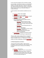
This text is intended to be supplementary to the official GAUSS manuals. Although the early
parts of the guide contain similar materials to the manuals (and some other online courses), my
aim here is to expound some principles of programming rather than explaining all GAUSS'
myriad features.
The reasoning behind this is simple. GAUSS is a complex language with a large number of
specialised functions for dealing with matrices. There are also a lot of add-on packages which
expand GAUSS's capabilities further. Attempting to cover all of these in detail in a single work
would be a mammoth undertaking. Moreover, it would be of limited value: it would have to
largely replicate the Reference Manuals, and it would not serve to deepen understanding of
GAUSS.
The rationale for this work is that a good grounding in programming methods makes a detailed
course on advanced features unnecessary. A competent user of GAUSS will find little difficulty
in interpreting the information in the manual on eigenvector calculations, for example; by
contrast, a user taught only how to use these functions may well be defeated by the task of
incorporating these functions in a useful program.
Hence, although this guide goes through the most fundamental parts of GAUSS in detail, more
advanced features get a relatively sketchy treatment. On the other hand, an increasing amount of
time is spent detailing approaches to programming. The emphasis in this coursebook is on
acquiring familiarity with the fundamentals of GAUSS and programming competence, rather
than becoming a GAUSS guru.
The first six sections of this guide (up to "Procedures") contain the core of GAUSS and should
be worked through. The last few ("Code refinements" onwards) are directed towards making
code more efficient, more readable, more easily maintained and more reliable. They can be
safely omitted but are recommended: a structured approach to coding is a transferable skill...
The functions referred to are introduced in connection with this knowledge-based approach. New
GAUSS users should be aware that there is a large body of routines available which are outwith
the scope of this guide.
Please note that this guide assumes some familiarity with elementary concepts in matrix algebra;
that is, readers should know the difference between scalars, matrices, and vectors, and
understand the basic matematical operations.
The web pages are designed for 800x600 and 1024x768 screens. The guide makes extensive use
of style sheets for layout. Unfortunately, these are poorly supported in many older browsers
including Netscape Navigator 4.7, which is common among Unix/Linux users. This site has been
designed for popular browsers that are relatively standards-compliant; that is, Internet Explorer
5.5, Netscape Communicator 6.1 and Opera 6.0, and all more recent versions. Apologies to those
on older browsers (especially Netscape 4.7), but as this is a free service I'm afraid I don't really
have the leisure to support all browser types. The text does remain readable, if rather ugly.
I hope you find this work useful. Please email comments to [email protected].
back to top
History
This manual was originally prepared in February 1994 for the seminars on Introductory GAUSS
Programming held in Stirling, Bristol and Glasgow, organised under the auspices of the CTI
Centre for Computing in Economics. A minor revision followed in 1995.
In April 1997 it was revised again and placed on the web as Word/WordPerfect documents with
PDF versions of the chapters. I also placed some code and programs on the web. Those of you
who visited the site at that point will no doubt have been astonished by my design skills. In my
defence, I will say that at this time I was writing one of the earliest academic websites in the
country; the only information about writing web pages was to be found on the CERN site itself.
For those wanting some light relief feel free to check out the web archive.
The gauss website http://scottie.stir.ac.uk/~fri01/gauss/ then stayed unchanged for the next five
years, as I moved between various jobs, eventually leaving academic economics for the
commercial sector. However, following my move to <A HREF="http://www.trigconsulting.c
Introduction
On this page: what is GAUSS? platforms and interfaces guide notation using GAUSS
Basic
operations
Introduction
Input and
output
Matrix algebra
and
manipulation
Program
control
Procedures
Code
refinements
Safer
programming
Writing for
posterity
Summary
remarks
1. What is GAUSS?
GAUSS is a programming language designed to operate with and on matrices. It is a general
purpose tool. As such, it is a long way from more specialised econometric packages. On a
spectrum which runs from the computer language C at one end to, say, the menu-driven
econometric program EViews at the other, GAUSS is very much at the programming end.
Using GAUSS thus calls for a very different approach to other packages. Although a number of
econometric add-ons have been written (for example, ML-GAUSS, a suite of maximum
likelihood applications), you will rarely be able to "turn up and go" with GAUSS. More often
than not, getting useful results from GAUSS requires thought, a systematic approach, and usually
a little time.
Having said that, the thought required is often no more than a recognition of what precisely you
are trying to achieve. The GAUSS operators and the standard library functions are designed to
work with matrices. This means that if you can write down the operations you want to perform,
the chances are that they can be translated directly into a line in your program. The statement "
β=(X'X)-1X'y" is acceptable to GAUSS with only minor changes.
1.1 Advantages
●
Preface
Home page
●
●
●
●
GAUSS is appropriate for a wider range of applications than standard econometric
packages because it is a general programming language.
GAUSS operates directly on matrices. This makes it more useful for economists than
standard programming languages where the basic data units are all scalars.
GAUSS programs and functions are all available to the user, and so the user is able to
change them. If you dislike a heteroscedasticity test in a commercially produced package,
you may be able to a new routine and replace the old procedure with your own.
Similarly, if data is held in a non-standard format, you may write your own routine to
access it.
GAUSS is extremely powerful for matrix manipulation. It is also fast and efficient.
1.2 Disadvantages
●
●
●
●
●
●
The fixed costs of using GAUSS are high. Its very generality means that there is unlikely
to be a simple procedure to do a simple econometric task readily to hand (although
commercially available routines ameliorate this somewhat).
Even if pre-programmed or bought in software is available for a task, a reasonable degree
of familiarity with GAUSS and its methods will often be necessary to make effective use
of such routines.
GAUSS is too tolerant of sloppy programming. GAUSS is very flexible; however, this
means it is difficult for the computer to tell when mistakes occur. For example, lax
conformability requirements mean that it is easy to mistakenly divide a scalar by a row
vector and then multiply by a matrix in the belief that all three variables were column
vectors.
GAUSS is not tolerant of errors in its environment. Ask it to read from a non-existent file,
or use an uninitialised variable, and the program stops. This is, of course, a sensible
feature of all programming languages. Unfortunately, GAUSS is short on routines
allowing non-fatal error checking.
Input and output routines are basic - especially input.
GAUSS programs are designed to be run within the GAUSS environment. They cannot be
run as stand-alone programs (.EXE files) without buying a program called the "GAUSS
EngineTM". Thus you can only swap code with other GAUSS users.
1.3 When to use GAUSS
GAUSS is ideally suited to non-standard tasks. For example, we have developed programs to
analyse and do estimates on data which comes in the form of cross-product matrices.
Alternatively, you may wish to vary or add to standard techniques; for example, adding a new
estimator.
If the core of your task is matrix manipulation in any way, then GAUSS is likely to be a better
bet than a full programming language. Its primitive I/O facilities are offset by the processing
capability. However, GAUSS is not appropriate for, say, writing a menu system; a generalpurpose language is probably easier.
Nor is GAUSS appropriate for standard applications on standard datasets. There is little point in
writing a probit estimation routine in GAUSS for a small dataset. Firstly, there are already
routines commercially available for non-linear estimation using GAUSS. More importantly, TSP,
LimDep, etc will already perform the estimation and there is no necessity to learn anything at all
about GAUSS to use these programs. However, to get extra specification tests, for example, a
straightforward solution would be to code a routine and emend the preexisting GAUSS probit
program to call the new procedure at the appropriate point in its working.
2. Platforms and interfaces
GAUSS is available in both single user versions and networked versions. From the user's
perspective, the main difference is that you may have less control over your environment in a
network setting, but otherwise the versions are the same. For the system administrator, the
network version simplifies license and user management, particularly for shared machines.
2.1 GAUSS on a PC
GAUSS for PCs now comes as a Windows application. However, for those wanting to use the
old DOS-based interface a program called TGAUSS.exe is included with the distribution. There
appears to be a negligible speed difference between the two.
2.2 GAUSS on Unix/Linux
GAUSS on Unix is very powerful and very quick, partly because Unix machines are designed for
heavy-duty processing and computation rather than user interaction. For manipulating large
matrices, the time saving can be tremendous.
GAUSS on Unix runs in both teletype (command-line) and X-Windows mode. Access to the
latter depends on how you access your Unix machine.
There is also a version to run on Linux (a form of Unix which runs on Intel processors). For
simplicity, this guide will not distinguish bewtween Unix and Linux.
2.3 Memory management
The amount of memory used by GAUSS can be varied by the user. GAUSS also provides an
option for "virtual memory", which is when disk space is used as "overflow" memory. In this
case, the apparent "memory" is only limited by the amount of free space on your disk. However,
using this extra disk space is much slower than using your machine's memory to store data, and,
while GAUSS will try to use memory in preference to disk space, poor use of data could result in
your program slowing down considerably.
In the early days of GAUSS, efficient memory management was often crucial to getting a
program running well. However, modern computers have far more memory and already use
virtual memory systems. As operating system memory-management facilities are efficient and
can be tailored to the specific machine, it is better in most circumstances to leave the computer to
sort its own memory requirements.
back to top
This does not mean you may ignore the issue of effective programming skills. It is suprisingly
easy to run out of memory when doing complex operations on large matrices. For a more
detailed discussion see the section on code refinements.
2.4 Interfaces
GAUSS programs can be written in two ways:
●
●
command-line
In this mode, commands typed into the GAUSS interface are executed immediately. This
allows for an instant response to a command, but the commands cannot be stored. This is
therefore not suitable for writing large programs, or for commands which need to be run
repeatedly.
batch or program
In this mode, GAUSS commands are typed into a text file. This file is then sent to be
GAUSS to be run. This allows one to develop and store complex programs.
This facility has existed since the earliest versions of GAUSS. However, the precise way this is
carried out has varied over time. The original DOS interface is still extant in the latest Windows
version as "TGAUSS", but the recommended interface is the windowing one. The Unix version
is closer to the DOS version but has a few operating differences. Additionally, all three versions
draw graphics windows differently as a result of their operating environments.
However, the practical differences between versions of GAUSS on various operating systems are
minimal. The GAUSS code covered in this guide should be universally applicable. Thus there is
no section of the guide concentrating on the interfaces. At the moment, I suggest you refer to the
manual for your particular version. In due course I hope to add an Appendix on GAUSS version
differences and interfaces.
3. Notation and layout
back to top
GAUSS is not case-sensitive. However, throughout the guide capitals will be used for 'reserved
words' and standard GAUSS functions. The names of all variables are lower case, with capital
letters separating words. Procedures will be identified by an initial capital. All this makes no
difference to GAUSS; it just makes life easier (see section on Writing for posterity). Italics will
be used to indicate a value to be substituted.
Where a constant is mentioned, this means an actual number or character set. Values are the
results of some operation. Where a constant is required, a constant must be supplied; but where a
value is required either a constant or a value is acceptable. Constant-list and value-list are lists
of constants or values, separated by spaces or punctuation marks. The type of separator may
affect the result of the operation.
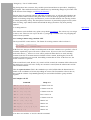
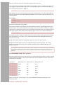
3.1 Examples
Naming conventions
LET
GAUSS reserved word
DELIF
GAUSS standard procedure
Process
user-defined procedure
FindFile
user-defined procedure
mat1
variable
fileName
variable
Constants
a
"a"
27
Invalid constants
"ok"
-0.0062
5.3E+2
a*b
c-27
Constant-lists
a b c d e
a, b, c,
"a", "b", "c"
1,2,3,4.5,6.7,8
1 2 3 4.5 6.7 "hello" 8
values
a
"a"
a*b
b+a
"ok"
5.3*102
5.3E+2
-27*(63+5)
value-lists
a*b, b*c, c*a
a*b 25 b*c "hello"
c*a
Note that, when constants are expected, a string constant (a piece of text) may or may not be
enclosed in quotation marks. It makes no difference to GAUSS, other than to make errors more
likely. By contrast, when a value is expected, a string without quotation marks will be treated as
a variable the current value of which is to be used. To try to avoid this confusion, this
coursebook will place string constants in quotation marks; strings with no quotation marks will
be variables.
For large numbers we use GAUSS's scientific notation standard; that is 5,720 can be written as
5.72E+3 (5.72 x 103) and 0.05 as 5.0E-2 (5.0 x 10-2).
3.2 Layout and Syntax
GAUSS could be described as a free-form structured language: structured because GAUSS is
designed to be broken down into easily-read chunks; free-form because there is no particular
layout for programs. Although the syntax is closely defined, extra spaces between words
(including line breaks) are ignored. Commands are separated by a semi-colon, rather than having
one command on each line as in FORTRAN or BASIC. A complete instruction is identified by
the placing of semicolons, and not by the placing of commands on different lines.
Program layout is generally a matter of supreme indifference to GAUSS, and this gives the user
freedom to lay out code in a style he finds acceptable. For example, the conditional branching
operation IF could be written
IF condition; action1; ELSE; action2; ENDIF;
but equally acceptable to GAUSS would be
IF condition;
action1;
ELSE;
action2;
ENDIF;
or
IF condition; action1;
ELSE; action2; ENDIF;
or
IF condition;
action1;
ELSE;
action2;
ENDIF;
The coursebook will use the leftmost of these formats, but this is a matter of personal choice and
users may wish to develop their own style. More will be made of this in Writing for posterity.
There are some exceptions to the rule that layout does not matter. Obviously, there cannot be
extraneous spaces within words or numbers: 'I F', 'var 1' and '27 000' are not the same as 'IF',
'var1' and '27000'. In more recent versions of GAUSS spaces within mathematical expressions
are not allowed in certain places, although this does not seem to be consistently enforced.
The other place where spacing is important is in comments:
/* this is a comment */
Anything within the /*...*/ markers is ignored by the program. However, there must not be a
space between the slash and the asterisk, or the program will not recognise a comment marker
and will erroneously try to analyse the contents of the comment block.
4. Using GAUSS
back to top
GAUSS in common with many other programs, will take instructions either from a file or from
the command line. To start GAUSS:
●
●
●
in Windows, start GAUSS from the start menu list of programs
in Unix, type "gauss"
for TGauss, either use the window start menus, or, in an MS-DOS box, go to the GAUSS
directory and type "tgauss". GAUSS 4.0 for Windows also installs a desktop icon which
you can click on.
In all cases, GAUSS is operating in a command line mode. As each instruction is typed in, it is
executed. A semi-colon is not necessary at the end of each line, although if you want to put
several instructions on a line you will need to separate them with semicolons. GAUSS will carry
out the instruction immediately.
To exit GAUSS, either close the window or type "QUIT" or "SYSTEM".
Command-line mode is fine for testing a few instructions, but for anything more than a couple of
lines of code it is more sensible to operate in batch mode. In this case, you type the instructions
into a separate text file, and then tell GAUSS to run the instructions in one go (a batch) with the
command
RUN fileName
This will execute all the instructions in the file fileName in sequence. The results are, in theory,
identical, whether the commands are in a file or typed in one at a time. The choice of when to
work at the command line and when to place instructions in a file depends on the problem at
hand; however, for more than a couple of lines of code, working in a file is usually easier.
Specific instructions as to how to edit and save text files depend upon your operating system. In
the rest of this guide "program" will refer to any self-contained body of code we are working on,
and you will find it easier to write the programs in separate files.
You can run programs directly without having to load GAUSS. At the Unix prompt, for example,
entering
gauss fileName
will load GAUSS and run the program automatically. If you do not include either SYSTEM or
QUIT and then end of our program then when the program has finished it will leave you in the
GAUSS environment.
[ previous page ] [ next page ]
Copyright © 2002 Trig Consulting Ltd
Introduction
On this page: variables creating matrices references managing data procedures
Basic
operations
Basic Operations
Input and
output
Matrix algebra
and
manipulation
Program
control
1. Variables
GAUSS variables are of two types: matrices and strings. There are also two ways of grouping
variables: structures and string arrays.
Matrices obviously include vectors (row and column) and scalars as sub-types, but these are all
treated the same by GAUSS. For example
a = b + c;
Procedures
Code
refinements
Safer
programming
Writing for
posterity
Summary
remarks
Preface
is valid whether a, b, and c are scalars, vectors, or matrices, assuming the variables are
conformable. However, the results of the operation may differ depending on the variable type.
Matrices may contain numerical data or character data or both. Eight bytes are used to store
each element of a matrix. Hence, each cell in a matrix can contain up to eight text characters, or
numerical data with a range of about 1.0E±35. If you enter text of more than eight characters into
the cells in a matrix, the text will be truncated. Numerical data are stored in scientific notation to
around 12 places of precision.
Strings are pieces of text of unlimited length. These are used to give information to the user. If
you try to assign a string value to an element of the matrix, all but the first eight characters will
be lost.
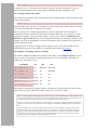
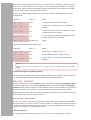
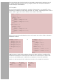
1.1 Examples of data types
Home page
●
●
●
●
4x3 Numerical matrix
1
2.2
-3
9
99
100
6.29E-6
5
7
1000
-5.3E+29
4
2x4 Character matrix
Will
Will
Harry
Steve
Harry
Dick
John
HarryIII
Edinburg
40
EH
Glasgow
25
G
Heriot-W
43
EH
Stirling
0
FK
Strathcl
23
G
5x3 Mixed matrix
Strings
"Hello Mum!"
"Strings are pieces of text of unlimited length"
"2.2"
""
Note the truncation of text in the character and mixed matrices. The null string "" is a valid piece
of text for both strings and matrices.
Because GAUSS treats all matrix data the same, GAUSS sometimes must be told that it is
dealing with character data. The $ sign identifies text and is used in a number of places. For
example, to display the value of the variable "v1" requires
PRINT v1;
PRINT $v1;
or
PRINT v1;
PRINT $v1;
depending on whether v1 is a numerical matrix, a character matrix, or a string. Strings are
identified by GAUSS and don't need the $. You can put one in if you like but it makes no
difference to printing.
Variables need to have names to reference them. Acceptable names for variables can contain
alphanumeric data and the underscore "_", and must not begin with a number . Reserved words
may not be used; standard procedure names may be reassigned, but this is not generally a good
idea. Variables names are not case-sensitive.
●
●
Acceptable variable names:
eric Eric eric1 eric_1 _eric1 _e_r_i_c
Unacceptable variable names:
1eric 100 if (reserved word) delif (GAUSS procedure - legal, but foolish)
1.2 Grouping variables
String arrays are, as the name suggests, a convenient way of grouping strings. They are similar
to a character matrix, but the strings they contain can be of unlimited length. Thus this is a valid
string array:
Aberdeen
Dundee
Edinburgh
Glasgow
Heriot-Watt
St. Andrews
Stirling
Strathclyde
Note how the data fields are more than eight characters long. One difference between a character
matrix and a string array is that GAUSS treats the former as a standard array so you can carry out
any matrix operation on it, whether it makes sense or not. In contrast, a lot of operations will not
be allowed on a string array because GAUSS 'understands' the string data type.
String arrays are therefore more flexible in storing characters. However, they have some
disadvantages. First, they only store strings, and therefore you cannot mix charcter and numeric
data. Second, because the length of the element is variable, GAUSS will handle them less
efficiently. If all your character strings are eight characters or less, then keeping them in a
character matrix may be marginally quicker. Third, string arrays take up more memory. For
example, a 32768-element character matrix takes roughly 270Kb, irrespective of the number of
characters. A string matrix with an average string length of 4 charaters takes 400Kb; with an
average length of eight characters that rises to 560Kb, twice as much as the equivalent character
matrix.
Structures allow the grouping of variables of different types. They were introduced in version
4.0. Suppose you are running repeated regressions and for each regression you want to store the
following information for each array:
Scalars:
TSS, ESS, RSS, σ, N
Vectors:
Coefficients, standard errors
String array List of variable names
By placing these into a structure, they could be passed around between procedures, simplifying
the program. This could also mean lower maintenance, by minimising changes to procedure calls
if the structure form changes; see Writing for Posterity.
Because these are grouping concepts rather than new data types, we will not deal with these any
further until the latter sections of the guide when we discuss better programming methods. For
details on declaring string arrays and structures, see the GAUSS manuals. One warning: neither
is treated particularly clearly. The description of structures is particularly opaque because (at the
time of writing, April 2002) both the manual and the help system have only been partially
updated.
2. Creating matrices
back to top
New matrices can be defined at any point (except inside procedures). The easiest way is to assign
a value to one. There are two ways to do this - by assigning a constant value or by assigning the
result of some operation.
2.1 Creating a matrix using constants: LET
The keyword LET creates matrices. The format for creating a matrix called varName is
LET varName = constant-list;
LET varName[r,c] = constant-list;
In the first case, the type of matrix created depends on how the constants were specified. A list of
constants separated by space will create a column vector. If, however, the list of constants is
enclosed in braces {}, then a row vector will be produced. When braces are used, inserting
commas in the list of constants instructs GAUSS to form a matrix, breaking the rows at the
commas. If curly braces are not used, then adding commas has no effect. In the first case, the
actual word 'LET' is optional.
If the second form is used, then an r by c matrix will be created; the constants will be allocated to
the matrix on a row-by-row basis. If only one constant is entered, then the whole matrix will be
filled with that number.
Note the square brackets. This is the standard way to tell GAUSS either the dimensions of a
matrix or the coordinates of a block, depending on context. The first number refers to the row,
the second the column. Curly braces generally are used within GAUSS to group variables
together.
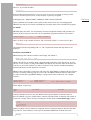
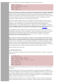
2.2 Examples of LET
Command
Shape of x
LET x = 1 2 3 4 5 6;
Column vector 6x1
LET x = 1,2,3, 4,5, 6;
Column vector 6x1
LET x = 1 2, 3 4, 5 6;
Column vector 6x1
LET x = {1 2 3 4 5 6};
Row vector 1x6
LET x = {1,2,3, 4,5, 6};
Column vector 6x1
LET x = {1 2, 3 4, 5 6};
Matrix 3x2
LET x[3,2] = 1 2 3 4 5 6;
Matrix 3x2
LET x[3,2] = 1, 2, 3, 4, 5, 6;
Matrix 3x2
LET x[3, 2] = 5;
Matrix 3x2
If we have two variables "a" and "b" then the command
LET x = a*b;
is illegal as "a*b" is a value and not a constant. In practice, GAUSS will interpret "a*b" as a
string constant and will create a string variable containing the letters and figures "a*b".
2.3 Creating a matrix using values
The results of any operation can be placed into a matrix without an LET explicit declaration. The
result of the operation
m1= m2 + m3;
will be that the value "m2+m3" is contained in a variable called "m1". If the variable m1 did not
exist before this statement, it will have been created.
The size and type of a variable depends entirely on the last thing done with it. Suppose m1
existed prior to the last operation. If m2 and m3 are both scalars, then m1 will now be a scalar regardless of whether it was previously a matrix, vector, scalar, or string. Variables have no
fixed size or type in GAUSS - they can be changed at will simply by assigning a different value
to them. It is up to the programmer to make sure he has the correct variable for any operation, as
GAUSS will rarely check.
Assigning a value is done by writing down the equation. Any correct (for GAUSS's syntax)
mathematical expression is acceptable, as are strings or the results of procedures.
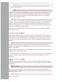
2.4 Examples of assigning values to a variable
The routines ZEROS and ONES create matrices of 0s and 1s. The transpose operator ' can be
used as in any normal equation. Examining the impact of various assignment statements on
matrices m1, m2 and m3 we get
Command
m1
m2
m3
m1 = ZEROS(2,3);
2x3
undefined undefined
m2 = ONES(1, 3);
2x3
1x3
undefined
m3 = m1*m2';
2x3
1x3
2x1
m1 = "Hello Mum!";
String 1x3
2x1
LET m2 = 5 2;
String 2x1
2x1
m3 = m3'*m2;
String 2x1
1x1
Note that LET statements can appear anywhere constants are used. The final size of m3 will be
governed by the result of the last operation; in this case, it becomes a scalar.
Why use constant assignments rather than just creating matrices as a result of mathematical or other operations? The
answer is that sometimes it is awkward to create matrices of appropriate shapes. It also allows for increased security,
as constant assignment is finicky about what values are appropriate, and will trap more errors.
However, you cannot rely on this. The above example of LET x = a*b giving a string variable rather than a numeric
variable is a simple of how GAUSS will do the correct thing, by its definition, and happily produce a meaningless
result.
In practice the main place you will use constant assignment will be at the beginning of programs where you set
initial values and environment variables (like the name of an output file, or font to use for graphing). During the
program you will be using variable assignment most of the time and you can ignore the strict rules on constants
assignment. However, this is one of those areas where unnoticed errors creep in, and you need to be aware that
GAUSS assigns values in different ways depending upon the context.
3. Referencing matrices
back to top
3.1 Direct references
Referencing strings is easy. They are one unit, indivisible. Matrices, on the other hand, are
composed of the individual cells, and access to these might be required. GAUSS provides ways
of accessing cells, columns, rows and blocks of the matrix as well as referring to the whole thing.
The general format is
mat[r1:r2,c1:c2]
where mat is the matrix and r1, r2, c1, and c2 may be constants, values, or other variables. This
will reference a block from row r1 to row r2, and from column c1 to column c2 of the matrix
mat. A value could be assigned to this block; or this block could be extracted for output or
transfer to some other location. For example,
mat = {1 2 3, 4 5 6, 7 8 9, 10 11 12};
PRINT mat[2:3,1:2];
would print the columns 1 to 2 of rows 2 to 3 of the matrix mat:
4
5
7
8
To reference only one row or one column, only one coordinate is needed in that dimension:
mat[r1,c1:c2]
or
mat[r1:r2,c1]
For example, to reference the cell in the third row and fourth column of the matrix mat, these
terms are all equivalent:
mat[3:3,4:4]
mat[3,4:4]
mat[3:3,4]
mat[3,4]
Entering "." or 0 as a co-ordinate instructs GAUSS to take the whole row or column of the
matrix. For example
mat[r1:r2,.]
means "rows r1 to r2 and all columns of matrix mat", while
mat[0, c1:c2]
references for columns c1 to c2. A whole matrix could then be referred to identically as
mat
or
mat[.,.]
This particular feature of GAUSS causes a number of unexpected problems, particularly when using loops to access
columns or rows in sequence. If your counter drops to zero (or some unspecified values) then you will find the
program operating on all rows or columns instead of just one.
For vectors only one co-ordinate is needed. For a column vector, say, these are all identical
mat[r1:r2,.]
mat[r1:r2,0]
mat[r1:r2,1]
mat[r1:r2]
For scalars there is obviously no need for co-ordinates. However, because a scalar is a subclass
of matrix,
mat[1,1]
mat[.,.]
mat[1]
mat[1,0]
or a number of other variations are acceptable.
This similarity in accessing matrices of zero, one, or two dimensions allows you to program
loops to access matrices without necessarily knowing the dimensionality of the matrix in
advance.
A last way to identify a set of rows or columns is to list them sequentially. For example, to refer
to columns 1, 3, and 22 and rows 2 to 4 inclusive of the matrix mat we could use
mat[2:4,1 3 22]
Note that that there are no separating commas in the list of columns; GAUSS treats everything
up to the comma as a row reference, everything afterwards as a column reference. If it finds two
or more commas within square brackets, it treats this as an error.
3.2 Indirect references
Elements of matrices can also be referred to indirectly. Instead of explicitly using a constant to
indicate a row or column number, a variable can also be used. For example,
PRINT mat[1:5, .];
and
endRow = 5;
PRINT mat[1:endRow, .];
are equivalent. This is a key feature in all but the most simple programs, as it avoids having to
write out references explicitly. For example, suppose the program is to print out ten lines of a
matrix. One solution would be to write a command to print each line:
PRINT mat[1,.];
PRINT mat[2,.];
...
This is clearly a tedious process. But one could write a loop to change the value of a variable i
from 1 to 10. Then, only one PRINT statement is need in the loop:
PRINT mat[i,.];
Even more usefully, this feature will work even if you are unsure how many lines there are in the
matrix. You can set the loop to go as many times round as there are lines in the matrix. The
PRINT statement does not have to be changed at all.
Similarly, instead of entering explicilty a list of column or row numbers to be selected, if you
enter a vector then GAUSS will use these as the indexes. For example, if rowv is a vector
containing (1, 2, 3) then
mat[1 2 3, .];
and
mat[rowv,.];
are equivalent.
3.3 Nested references
This section is in here to complete coverage of referencing matrices. It is more advanced, and can be skipped at this
point.
Indirect references could be nested. If rowv and colv are a vectors of numbers, then
mat[rowv[1]:rowv[2], .]
is legal. So is
mat[rowv[r1,c1]:rowv[r2,c2], colv[rowv[r3, c3], rowv[r4,c4]]]
if values have been assigned to r1, c1... and the matrices row and col have the relevant
dimensions. This process can be carried on infinitum.
However, one problem with this flexibility in referencing is that GAUSS will always try to find a
solution. For example, to access the first row of matrix mat you could use the vector rowv
(above), one could use
mat[rowv[1],.]
However, if you omit the index
mat[rowv,.]
then GAUSS will interpret this row vector as a list of rows to be selected, as in the previous
section. It will not report an error, as this construct is perfectly acceptable
4. Managing data - SHOW, PRINT, FORMAT, NEW, CLEAR, DELETE
These commands are introduced at this point as they are the basic ones for managing data.
DELETE may only be used at the command line, but all the others can be included in programs.
4.1 SHOW
SHOW displays the name, size and memory location of all global variables and procedures in
memory at any moment (see Section 6 for an explanation of global variables). The format is
SHOW varName;
or
SHOW/m varName ;
where varName is the variable of interest. The "wild card" symbol "*" can be used, so that
SHOW er* ;
will find all references beginning with "er". The /m parameter means that only matrices are
displayed.
4.2 PRINT and FORMAT
PRINT displays the contents of matrices and strings. The format is
PRINT var1 var2 var3... varx ;
which prints the list of variables. How it prints depends on the data. If the data fits on one line
(all row vectors, scalars, or strings) then PRINT will display one after the other on the same line.
If, however, one of the variables is a matrix or column vector, then the variable immediately
following the matrix will be printed on a new line.
PRINT wraps round when it reaches the end of the line. Each PRINT command will start off on a
new line. To display without going on to a new line, the PRINT statement must be ended with
two semi-colons; this stops PRINT adding a carriage return to the variable list. For example,
consider
PRINT "Hello";
PRINT "Mum";
and
PRINT "Hello";;
PRINT "Mum";
and
PRINT "Hello" "Mum";
These display, respectively,
Hello
Mum
HelloMum
HelloMum
If string constants (as above) are used, PRINT will recognise that this is character data. If,
however, PRINT is given a variable name, it must be informed if this is character data (either in
a matrix or a string). This is done by prefixing the variable name with the dollar sign $. Hence
a = 1;
b = 3;
c = "letters";
PRINT a b $c;
prints everything correctly. Matrices composed entirely of character data are shown in the same
way; however, mixed matrices need a special command, PRINTFM, of which more later.
Warning
back to top
Once GAUSS comes across a $ sign indicating character data, it prints all the rest of that line as text. Thus
PRINT a $c b;
would lead to 'b' being treated as if it were text. To get round this, 'b' must be printed in a separate statement,
perhaps using the double-colon:
PRINT a $c;;
PRINT b;
PRINT style is controlled by the FORMAT commands, which sets the way matrices (but not
strings) are printed. There are options to print numbers and character data with varying field
widths, decimal expansion, justification, spacing and punctuation. These are covered in the
manual and are all similar in form to:
FORMAT /RD 6, 0;
where, in this case, we have numbers right-justified (/RD), separated by spaces (/RDC would do
commas), with 6 spaces left for writing the number and 0 decimal places. If the number is too
large to fit into the space, then the field will be expanded but for that number only - not the
whole matrix. Strings are given as much space as they need, but no spaces are inserted between
them (see the "HelloMum" example, above).
The print styles set by FORMAT operate from the time they are set until the next FORMAT
command is recieved.
4.3 NEW, CLEAR, and DELETE
These three all clean up memory. They do not affect files on disk. NEW clears all references
from memory. It can be called from inside a program, but obviously this is rarely a smart move.
The exception is at the start of a program. A call to NEW will remove any junk left over from
previous work, leaving all memory free for the new program. NEW has no parameters and is
called by
NEW;
Calling NEW at the start of a program ensures that the workspace is cleared of unwanted
variables, and is good practice. Calling NEW at any other point is usually disastrous and not so
highly recommended.
CLEAR sets particular variables to zero, and it can also be called by a program. It is useful for
tidying up data and initialising variables:
CLEAR var1 var2 ... varN ;
Because it sets the variable to the scalar zero, then CLEAR is identically equal to a direct
assignment:
CLEAR x;
is equivalent to x
= 0;
DELETE clears variables from memory, and so is a better option than CLEAR for tidying up
unwanted variables. However, it cannot be called from inside a program. The delete command is
like SHOW:
DELETE varName;
DELETE/n varName;
where varName can include the wild card character. The /n option stops GAUSS doublechecking the deletion is wanted. The special word "ALL" can be used instead of varName; this
deletes all references, and so
DELETE/N ALL;
is equivalent to NEW.
5. Using procedures
back to top
The library functions in GAUSS work like library routines in other packages - a procedure is
called with some parameters, something happens, and a result may be returned. The parameters
may be constants or variables; any returned values must be placed in variables. There may be any
number of input and output parameters, including none. The general format is
{outVar1, ...outVarN} = ProcName (inVar1, ... inVarN);
The inVar parameters are giving information to the procedure; the outVar variables are
collecting information from the procedure. The input parameters will be unaffected by the
action of the procedure (unless, of course, they also feature in the output list). The outVar
parameters will be affected, and so obviously constants can not be used:
{outVar1, "eric"} = ThisProc (inVar1, inVar2);
is incorrect.
Note that we have curly brackets {} to group variables together for the purposes of collecting
results, but that we have round brackets () to delineate the input parameters. The former is
GAUSS's usual way of grouping things together, the latter is a near-universal programming
syntax. They're mixed in together just to keep you on your toes.
If there is one or no parameter, then the form can be simplified:
{outVar1, ... outVarx} = ProcName (inVar);
one input parameter
{outVar1, ... outVarx} = ProcName;
no input parameter
ProcName (inVar1, ... inVarx);
no returned result
outVar = ProcName (inVar1, ...inVarx);
one result returned
For example, the procedure DELIF requires two input parameters (a matrix and a column
vector), and returns one output, a matrix:
outMat = DELIF (inMat, colVec);
The procedure EIGCG requires two input parameters and two output parameters
{eigsReal, eigsImag} = EIGCG(matReal, matImag);
The procedure SORT needs four input parameters but returns no result:
SORT (inFile, outFile, keyName, keyType);
If the program is not concerned with the results from procedure then the function CALL tells
GAUSS to throw away any returns. This can save time and memory in some cases. For example,
the quickest way to find the determinant of a large matrix is through a Cholesky decomposition.
Running the procedure CHOL sets a global variable which can be read by the procedure DETL
to give the matrix's determinant. However, the actual result of the decomposition is not wanted,
only a side effect. So, to find the determinant of mat most quickly use
CALL CHOL(mat);
determ = DETL;
As input and returned parameters are both lists, you can pass the whole list of returned
parameters to a new function, along with any other parameters that are necessary. This means
that you do not need to have any intermediate variables to store the results from one procedure
before passing them to another, and it will make your code shorter. However, it will not
necessarily make it more readable, and you can run into maintenance problems - if you change
the list of parameters for one procedure you need to change it for the other as well.
Warning
For all procedures, it is the programmer's responsibility to ensure that the right sort of data is used. If a procedure is
expecting a scalar as a parameter and you pass it a row vector, for example, this will not be flagged as an error when
GAUSS checks the program syntax. It may or may not cause the procedure to crash but this will not be apparent
until the program is running. All GAUSS will check is that the correct number of parameters is being passed back
and forth.
[ previous page ] [ next page ]
Copyright © 2002 Trig Consulting Ltd
Introduction
On this page: storing matrices datasets text files keyboard input spreadsheets graphics
Basic
operations
Input and output
Input and
output
Matrix algebra
and
manipulation
Program
control
GAUSS handles data on disk in a number of formats. It can read and create standard text files
and older spreadsheet formats, as well as using its own format to store matrices, datasets or code
samples.
In this section we shall also be covering briefly GAUSS's graphing capability.
1 Storing matrices (.fmt files)
Procedures
GAUSS stores matrices in files with a .fmt extension. This is the default option - if no extension
is given to file names, GAUSS will assume it is reading or writing a matrix file.
Code
refinements
The commands for matrix files are
Safer
programming
Writing for
posterity
Summary
remarks
Preface
Home page
LOAD varName = fileName;
LOADM varName = fileName;
SAVE fileName = varName;
LOAD and LOADM are synonyms. The reason for using the latter is that there are other similar
commands (LOADP, LOADS, LOADF, LOADK) which load different types of object (see
LOAD in the manual). LOADM tells GAUSS that a matrix is being loaded, and so it will check
other references accessing that variable to ensure that only legal operations are being carried out.
varName is the name of the variable in memory to be saved or loaded.; fileName is the name of
the matrix file with no .fmt extension. For example,
SAVE "file1" = mat1;
LOADM mat2 = "file1";
creates a file on disk called file1.fmt which contains the matrix mat1. This is then read into a new
matrix, mat2.
If the disk file has the same name as the variable, then fileName can be omitted:
LOADM eric;
SAVE lucy;
will load the matrix eric from the file eric.fmt, and then save the matrix lucy to a file called
lucy.fmt.
An alternative is to have the name of the file in a string variable. To tell GAUSS that the name is
contained in the string, the caret (^) operator has to be used. GAUSS then looks at the current
value of the variable to see which name to use, instead of taking the variable name as a constant
value. For example,
fileName = "file1";
LOADM mat1 = ^fileName;
fileName = "file2";
SAVE ^fileName = mat1;
This piece of code reads a matrix from file1.fmt and then saves it to file2.fmt. If the caret was
left out, then GAUSS would be looking for files called "fileName". This indirect referencing is
the more usual way of using file names: it allows for the program to prompt for names, rather
than having them explicitly coded into the program. This is useful when the program does not
know what files are to be used - for example, if a program is to be run on several sets of data.
You can also save GAUSS procedures, strings et cetera in the same manner, using variations on
the LOAD command. See the Command Reference for details.
2 Datasets (.dat files)
GAUSS datasets are created by writing data from GAUSS or by taking an ASCII file and
converting through a stand-alone program called ATOG.EXE (Ascii TO Gauss). As with the
datasets for other econometric packages, they consist of rows of data split into fields. GAUSS
will automatically add .dat to the filenames you give, and so there is no need to include the
extension.
In older versions of GAUSS the actual dataset is held in a .dat (data) file, while a .dht (header) file contains the
names of each of these fields, along with some other information about the data file. A program, Transdat, converts
between data formats, as well as between different operating systems.
For information on ATOG, see the GAUSS User Guide (not the Command Reference).
Unlike the GAUSS matrices, reading from or writing to a GAUSS dataset is not a single, simple
operation. For matrices, the whole object is being moved into memory or onto disk. By contrast,
a GAUSS dataset is used in a number of stages. Firstly, the file must be opened; then it may be
read from or written to, which may involve the whole file or just a few lines; finally, when
references to the file are finished, it should be closed.
All files used will be given a handle by GAUSS; this is a scalar which is GAUSS's internal
reference for that file. It will be needed for all operations on that file, and so should not be
altered. The handle is needed because several files can be 'open' at one time (for example,
reading from one, writing to another); precisely how many depends on the computer's
configuration. Without the file handle, a dataset cannot be accessed, and if the file handle is
overwritten then the wrong file may be used. So be careful with your handles.
2.1 Creating new datasets
A file must exist before it can be opened. To start a new dataset for writing, it must be created.
This is done by
CREATE handle = fileName WITH colNames, columns, type;
handle is the handle GAUSS will return if it is successful in creating fileName. This fileName
may be a constant like "file1", or it may be a string, referenced using the ^ operator (as for
LOAD and SAVE). colNames is the list of names for the columns (usually a character vector) ;
columns tells GAUSS how many columns of data there are (which is not necessarily the same as
the number of names - it may be sensible to have some "spare" columns); and type is the storage
precision of the data - integers, single precision, or double precision. For example,
fileName = "file1";
varNames = "Name" "age" "sex" "wage";
CREATE handle1 = ^fileName WITH ^varNames, 4, 4;
prepares a datafile called file1.dat for writing. A header file file1.dht will also be created, which
records that the datafile should contain four columns, named "Name", "age", "sex" and "wage",
and in single precision (type=4, the default).
CREATE is not needed very often - only when writing a brand new dataset. More usually
datasets are ATOG conversions from ASCII files. Alternatively, matrices may be converted into
datasets using the command
success = SAVED (variable, fileName, colNames);
where variable is the matrix to be saved, fileName and colNames are above, and success is a
scalar variable set to true if the operation worked.
2.2 Opening datasets
A dataset must be opened for either reading or writing or "updating" (both). Once a dataset has
been opened for one "mode" it cannot be switched to another. The command is
back to top
OPEN handle = fileName FOR mode VARINDXI offset
handle is a non-negative scalar, the file handle returned to you if the operation is successful (if
the command did not work, the handle is set to -1). The file handle should always be set to zero
before this command, to avoid the possibility of GAUSS trying to open a file already open.
fileName is as above.
The mode is one of READ, APPEND, or UPDATE. If the mode is omitted, GAUSS defaults to
READ. If READ is chosen, updating the file is not allowed. Choosing APPEND means that data
can only be appended to the file; the existing contenst cannot be read. UPDATE allows reading
and writing.
When GAUSS opens the file with VARINDXI, it reads the names of fields (columns) and
prefixes them all with "i" (for index). These can then be used to reference the columns of the
dataset symbolically instead of using column numbers explicitly. This makes programs more
readable, more easily adapted, and less likely to be upset by changes in the structure of the
dataset.
In the above example, the four columns in the dataset created could be referred to as 1 to 4 or,
equivalently but much more usefully, as iname, iage, isex, iwage. Using these index variables
without VARINDXI causes some problems for GAUSS when it is checking a program prior to
running it, so although VARINDXI is optional it should generally be included.
The offset scalar option shifts all these indexes by a scalar and so is useful if the data is to be
concatenated horizontally to another matrix or dataset. However, usually it can be left out.
When a file is CREATEd, it is automatically opened in APPEND mode (obviously; there is
nothing to be read as yet). However, creating new datasets is much rarer than accessing a
preexisting dataset, and so OPEN is more common than CREATE.
As an example, to open the file created in the previous sub-section for reading, the command
would be
OPEN handle1 = "file1" FOR READ VARINDXI;
which would give a file handle in handle1, and four scalar indexes: iname, iage, isex, and iwage,
set to 1, 2, 3, and 4 respectively.
2.3 Reading, writing, and moving about
Econometric packages tend to treat datasets as single entity, albeit with elements that can be
altered. For example, the TSP commands LOAD and SAVE are much more akin to the GAUSS
matrix file loading and saving (there are GAUSS commands LOADD and SAVED which
perform similar operations, but these are not covered here).
By contrast, a GAUSS dataset is explicitly composed of rows of data, and these rows are the
basic unit of manipulation. One or more rows is read at a time; data is parcelled up into rows
before being written. GAUSS maintains a file pointer which maintains the current position (ie
row number) in the file. Generally, as rows are read from or written to the file, the row pointer is
moved on. If the row pointer currently points to the start of the file and ten rows are read, the row
pointer now indicates that row eleven is the current row.
Reading and writing thus moves sequentially through the file. To move around the file, or to find
out where the file pointer currently is, use
currPos = SEEKR (handle, rowNum);
handle is the handle returned by OPEN or CREATE. rowNum is the row number to which the
file pointer is to be moved; if it is set to -1, then SEEKR will not move the file position. This is
useful because, whatever the value of rowNum, currPos is now a scalar holding the current row
number. Thus setting rowNum to -1 can be used to determine the current position. So, to move,
for example, five rows back in the file requires finding out the current row number and then
resetting the file pointer:
currPos = SEEKR (handle, -1);
currPos = SEEKR (handle, currPos-5);
After this operation, currPos should show that the file pointer has been moved back five rows.
Trying to move before the start or after the end of a file will cause the program to crash: GAUSS
will not be able to trap this error. The function ROWSF giving the number of rows in a file can
be used to avoid this error).
To read data, the command is
dataMat = READR (handle, numLines);
which reads numLines rows from the file referenced by handle into the data matrix dataMat.
After the read, the file pointer will have been moved on to point to the first row after the block
just read. Rows and columns in the dataset become rows and columns in the matrix. So, in our
above example,
dataMat1 = READR (handle, 10);
reads ten lines from the dataset and creates a 10x4 matrix called dataMat1 which can be accessed
like any other variable; the file pointer has been moved on ten rows.
GAUSS will not check for end-of-file; this has to be done by the user. Attempting to read past
the end of the file will cause the program to crash. This can be avoided by using a standard
procedure called EOF:
atEof = EOF(handle);
which sets atEof to true if the file pointer is at the end of file handle and false otherwise.
Writing data is just the reverse. The command
result = WRITER (handle, dataMat);
will try to add dataMat into the file at the current file position. dataMat must have the same
number of columns as the data currently in the file, or GAUSS will fail. Data in the dataset will
be overwritten, and the file pointer will be moved on to just after the written block. If the file
pointer is currently at the end of the file, the extra rows will be appended to the file. Thus,
existing datasets can only be added to at the end; odd rows cannot be inserted (except by some
particularly astute or wilful programming).
result is the number of lines actually written to disk. If result is less than the number of rows in
dataMat, then clearly something has gone wrong with the write operation - possibly disk full, or
trying to write to a read-only file. Thus the operation
numWrit = WRITER (handle, dataMat1);
using the 10x4 matrix read above should lead to numWrit being equal to 10; if not, something
has gone wrong.
The column names stored with the dataset can be used to refer to the matrix columns by using
the "i" prefix and the names. Thus, to print all the "name" and "sex" fields in the example matrix,
two equivalent commands are
PRINT $dataMat1[., 1] dataMat1[., 3];
PRINT $dataMat1[., iname] dataMat1[., isex];
but the second form is clearly much more readable. It also makes for more easily maintained
programs, as changes to the dataset will not affect the symbolic column references - GAUSS will
make sure "isex" and "iname" refer to the right column.
2.4 Closing datasets
Files should always be closed when reading or writing is finished. GAUSS will automatically do
this when leaving the GAUSS environment or when it encounters an END statement (see Section
5, Program Control). However, having files open unnecessarily may slow the system down; may
prevent new (and useful) files being opened; may be mistakenly altered by the program; and may
be corrupted or lose data due to system failure.
Files are closed by the CLOSE command:
result = CLOSE (handle);
If the file for handle was closed successfully, then result will be set to 0; otherwise, it will be -1.
The reason the handle is set to 0 on success and -1 on failure is because valid handles are all
positive numbers; therefore, GAUSS uses zero and negative numbers to indicate the state of the
file handle. If the CLOSE worked, then handle should be set to zero, to signify that there is no
open file attached with this handle (this information is used by OPEN and CREATE). This could
be combined by using
handle = CLOSE (handle);
as recommended by the GAUSS manual. However, if this operation is unsuccessful, then the
above formulation means that the original value of the handle is lost. A better option is to use a
temporary variable and test it; for example,
result = CLOSE (handle1);
IF result == 0;
handle1 = 0;
ELSE;
PRINT "Close failed on file number " handle1;
ENDIF;
This also allows a meaningful error message to be displayed. Note that this use of 0 or -1 is
inconsistent with the definition of true and false as 0 and 1; however, if you use false/not-false
(as recommended earlier) then logical operators will operate correctly. Another reason to use
zero/non-zero rather than relying on 0/1 for Boolean operations...
An alternative is to use one of the following:
CLOSEALL;
CLOSEALL handle1, handle2, ... handlex;
which closes all or a specified list of files. The first form does not set file handles to zero; this
should still be done by the program. The second form sets handles to zero, but GAUSS is silent
on the possibility of the closure failing.
3 Text files
Input can be taken from ASCII (i.e. normal alphanumeric text) files using the LOAD command
described above. This is augmented by the addition of square brackets which indicate the ASCII
nature of the file:
LOAD varName[] = fileName;
LOAD varName[r, c] = fileName;
In the first case, GAUSS will load the contents of fileName into the column vector varName,
which can then be checked for size and reshaped. This is the preferred option for loading ASCII
files. Items can be numeric or text and should be separated by spaces or commas. Line breaks are
treated as white space: GAUSS does not use them to distinguish rows. Text items longer than
eight characters will be truncated.
The second form loads the file into an r by c matrix. If there are too many elements in the file for
the matrix, then the extra ones will not be read; if the file does not contain enough data items,
then the ones found will be repeated until the matrix is full.
3.1 ASCII input examples
Supposing the file "eric.txt" contained
back to top
loaves 5
fishes 2
fishermen 2
Then
LOAD menu1[] = "eric.txt";
LOAD menu2[2, 2] = "eric.txt";
LOAD menu3[4, 2] = "eric.txt";
produces a 6x1 column vector called menu1 and two matrices called menu2 and menu3:
menu1
menu2
menu3
loaves
loaves 5.0
loaves
5.0
5.0
fishes 2.0
fishes
2.0
fishes
fishermen 2.0
2.0
loaves
5.0
fisherme
2.0
Note the truncation of "fishermen", and the lack of quote marks around the text items. Quote
marks would have been acceptable to GAUSS.
3.2 RESHAPE
RESHAPE is a standard GAUSS function which changes the shape of the matrix. The format is
newMat = RESHAPE (oldMat, r, c);
where newMat is now an r by c matrix formed from the elements of oldMat. If newMat and
oldMat do not have the same number of elements, then the rules for filling up the matrix are as
for the LOAD command. Thus these two pieces of code are equivalent:
LOAD tempMat[] = "eric.txt";
menu = RESHAPE (tempMat, 3, 2);
or
LOAD menu[3, 2] = "eric.txt";
but the first is a better solution. It allows for checking the number of elements read, which can be
used to test for errors in the input data.
Warning
Neither RESHAPE or LOAD[r, c] will send an error message if they do not find the correct number of elements to
fill the output matrix. They will always return a matrix of the desired size. This is why it is important to check the
number of elements read in before reshaping them into a matrix.
3.3 ASCII Output
Producing ASCII output files is no different from displaying on the screen. GAUSS allows for
all output to be copied and redirected to a disk file. Thus anything which appears on the screen
also appears in the disk file. To produce an ASCII file therefore requires that (i) an output file is
opened; (ii) PRINT is used to display all the information to go into the output file (iii) the output
file is closed when no more output is to be sent to it.
The relevant command to begin this process is OUTPUT:
OUTPUT FILE = fileName ON;
OUTPUT FILE = fileName RESET;
Both will instruct GAUSS to send a copy of everything it displays, from that point onward, to the
file fileName. If fileName does not already exist, then these two are identical; but if the file does
exist, then the first form ensures that any output is appended to the existing contents of the file,
while the second empties the file before GAUSS starts writing to it. If no file name is given, then
GAUSS will use the default "output.out". There is no default extension for output files.
Once a file has been opened, it can be closed and opened any number of times by combining the
above commands with
OUTPUT OFF;
These commands will all work on the last recorded file name given. The FILE=fileName bit
could be included here as well if the user wishes to swap between different output files;
generally, however, only one output file is used for a program, and so naming the file explicitly
is superfluous.
An analogous command SCREEN switches screen output on and off. These two commands are
independent and so screen display off and file output on is a perfectly acceptable combination.
3.3.1 Example uses of OUTPUT
Example 1 sends output to one file only, "eric.txt"; Example 2 sends output to two different files,
"eric1.txt" and "eric2.txt":
Example 1
Example 2
OUTPUT
:
OUTPUT
:
OUTPUT
:
OUTPUT
:
OUTPUT
:
OUTPUT
:
OUTPUT
:
OUTPUT
:
OUTPUT
:
OUTPUT
:
FILE="eric.txt" RESET;
OFF:
ON;
OFF
ON;
FILE= "eric1.txt" RESET;
OFF;
FILE="eric2.txt" RESET;
OFF;
FILE="eric1.txt" ON;
3.3.2 OUTWIDTH
Because GAUSS is treating the output as something to be "displayed" (even if only to a file), it
retains the concept of only having a certain number of characters on a "line". The default is
eighty characters, the standard screen width. This means that sending a matrix with a large
number of columns to an output file may lead to the matrix being broken up, with "overflow"
columns being put on new lines. The way to avoid this is to use
OUTWIDTH numChars;
where numChars is the nominal line width, and can be anything from 2 to 256. If this is set to
256, then this tells GAUSS to leave out all extraneous line breaks - new lines will only start with
a new row of the matrix.
Note that output on the screen may still be wrapped around. This does not affect the layout of the
output file - it is just the display's functionality, and nothing to do with GAUSS.
4 Keyboard input
GAUSS take input directly from the keyboard through two functions:
string = CONS;
mat = CON(r, c);
The first of these reads in a string variable, pure and simple. The second reads elements for a
matrix of dimension r by c, and works differently in different versions of GAUSS.
In GAUSS versions prior to 4.0, CON will prompt the user with a question mark and will treat
all white space as merely separating matrix elements. Thus, the CON command will read exactly
r by c elements; it will not let the program continue until it has read enough data points. It will
also break off the moment it has enough items. Suppose the program was given the instruction
data = CON(2, 3);
back to top
and the user attempted to enter
0123456
GAUSS would stop when it had read the "5". The fact that there was another item to be read is
irrelevant to filling a 2x3 matrix. If the user types ahead and is not aware that GAUSS has filled
the CON matrix, then the "6" will be read as the first bit of input next time any console input is
required.
Moreover, CON will not allow editing of the data already entered. If the user entered the above
sequence and then decided that 0 should be changed to 1, CON will not allow it. As each item is
entered, CON notes it, stores it, and moves on to the next item. There is no going back. This
means that program employing CON should make any unsuspecting user aware of the
importance of getting input right first time. This theme will be returned to in later sections.
GAUSS 4.0 has a vastly improved matrix editor, and it uses this to underpin CON. In GAUSS
4.0 the user is given co-ordinates, can edit numbers, and can also enter strings. The downside is
that the system is even more opaque to a new user; for example, there is no obvious way to get
out of the editor (enter 'x' in a cell). There is help available by typing '?', but if you want an
inexperienced user to run your program then you must give them adequate instructions.
Unix input varies because of the way distributed systems handle input streams. You may find
that the system does nothing until carriage return (the 'enter' key) is pressed.
All in all, CON is to be avoided in all systems except 4.0, and then only with good reason and clear instructions.
CONS allows you to read in data flexibly and analyse it, and GAUSS has routines to turn strings containing
numbers into matrices. For an example, see some of the procedures in the file datautil.gl.
5 Spreadsheets, database files, and other product formats
GAUSS 4.0 for Windows can import data from a variety of native file formats, including Lotus,
Excel, Quattro and dBase files. It uses the filename extension as a clue to the type of file,
although these can be overridden. For multiple-page spreadsheets, you can specify both the sheet
and the cell range to upload. If the first row contains text, GAUSS assumes that these are column
headings and creates an appropriate matrix of variable names. If it only finds numeric data, it
creates a vector of column names as "C1", "C2" and so on.
GAUSS will also export data to these third-party formats. However, it writes these data files in
the earliest compatible version. For example, although it understands Excel spreadsheets up to
version 7, it will save them as version 2.1 by default.
Using the IMPORT and EXPORT function is much more convenient than using ASCII files as
intermediaries, as well as being more reliable. However, if you are running your program on
something other than GAUSS 4.0 for Windows, you will need to go back to ASCII files for data
exchange.
If you are using Unix, do not have the latest version of GAUSS, or wish to access data in several
different formats, then the excellent program DMBS/Copy from Conceptual Software will
translate GAUSS matrices and datasets on disk into several spreadsheet formats, as well as all
the other major statistical packages. It is cross-platform, extremely easy to use and highly
recommended.
back to top
6 Graphics
One feature of GAUSS I/O that performs well is the graphing package. The way GAUSS draws a
graph is to provide functions which draw the graphs and only draw the graphs. All other
attributes are set using variables. So, to create a graph involves setting one variable to the title,
another to the type of lines wanted, another to the colour scheme, another to the scaling of the y
axis, and so on. When all this has been done, the relevant graph function is called, and it uses all
the information previously set to draw the graph with the right characteristics.
6.1 Essential preparations
Any program drawing graphs needs to have the line
LIBRARY PGRAPH;
in it. This should go at the start of the program. This tells GAUSS where all the specialised graphdrawing routines are to be found. If this line is omitted, graphs cannot be drawn.
The LIBRARY line should only appear once, but
GRAPHSET;
can be called repeatedly. This resets all the graph variables back to their default values.
Obviously, this should appear before the options for the next graph are written; otherwise any
options chosen will be reset to the defaults. Note that this is not a necessary statement; it is an
easy method of returning all settings to their default values. It is recommended you do this at the
beginning of the program as well to clear any settings left over frmo previous programs.
6.2 Options to be set
There are an enormous amount of options to be set - almost eighty. These are all detailed in the
System and Graphics Manual. They all begin with "_p" to make them easily identifiable. These
are set just like any other variables - the manual details what information is to be expected in
each. For example, consider the instructions
_pcolor = ZEROS(2,1);
_pcolor[1] = col1;
_pcolor[2] = col2;
:
_pbartyp = {2 1, 2 2, 2 3};
The _pcolor instruction sets colours for the XY and XYZ graphs. It is a 2x1 vector implying, in
this case, that there are two series to be plotted. The first series will be plotted in the colour
"col1", the second in "col2", both of which are variables.
The _pbartype instruction sets the shading type and colour for a bar graph. It is a 3x2 matrix,
implying three series. The first column in all three rows is 2 in this example, meaning that the
bars have vertical cross-hatching for all three series. The second column is colour: series one to
three are displayed in colours 1, 2, and 3 (what these colours actually mean on screen depends on
the user's machine).
The most useful variable is
_plegstr = "legend A\000legend B\000Legend C";
This defines legends for each line when a graph is displaying multiple series - three in this case.
The legends for each series must be separated by the code "\000". This is a null character telling
GAUSS that one name has ended and another is beginning.
The relevant variables to be set are detailed with each graph type. In addition there are a number
of general functions which control other settings, of which the most important are
TITLE(title);
XTICS(min, max, increment, subDivs);
XLABEL(title);
back to top
The first of these sets the title for the graph. XTICS (and the associated functions YTICS and
ZTICS) allow for scaling of the X-axis. If this function is not called, GAUSS will work out its
own scaling. min and max are the minimum and maximum values on the scale, with the scale
increasing by increment; negative values for the increment are acceptable. subDivs is the number
of minor ticks between each increment. Finally, XLABEL (and YLABEL and ZLABEL)
provides a title for the X-axis.
All these options should be set before printing a graph. However, most of the defaults are quite
sensible, and many options will not need changing. The defaults can be changed to the user's
preference too; they are all in a file called PGRAPH.DEC (see the manual for details).
6.3 Displaying and printing graphs
GAUSS provides a number of graph types, including bar graphs, X-Y, log X-Y and histograms.
All data for graphs comes in the form of matrices. When GAUSS finds a graph instruction, it
displays the graph immediately using the current set of options or defaults. This is why all
the options are set first. By the time GAUSS reaches a graph instruction, all it needs to produce
the graph is the data given in the function call.
The graph data are in NxK matrices, where N is the number of data points and K is the number
of series to be plotted. Whether multiple series are permitted or not depends on the graph: for
example, multiple series are allowed in an X-Y graph. So
xSeries = SEQA(1, 1, 20);
ySeries = ZEROS(20, 3);
ySeries[., 1] = thisData;
ySeries[., 2] = thatData;
ySeries[., 3] = otherDat;
XY(xSeries, ySeries);
will plot an X-Y graph consisting three series, each of 20 data points. The series are the values
held in thisData, thatData, and otherDat.
How the graph is displayed depends upon both the operating system and the version of GAUSS.
In the original DOS version, the graph is displayed full-screen and then remains on screen until
a key is pressed. The escape key (ESC) lets the program continue, while others bring up menus
for zooming into, printing or saving to disk the graph.
In early Unix versions, there was no graph displaying. Graphical files were simply saved to
disk.
In later Unix versions (designed for X-windows) and GAUSS for Windows, GAUSS included
functions to create graphical windows and place the results inside them. The user could direct
graph output to particular windows. Printing and saving was part of the window function.
In the most recent Windows version (4.0) a number of the windowing commands are
deprecated as GAUSS automatically creates graphical windows. This simplifies displaying
enormously. The graphical windows also have a much wider range of tools for dealing the
windows, sensibly organised. In particualr, saving graphs in other formats is relatively simple.
6.4 Using graphs in other programs
The graph can be saved to disk in a number of picture formats which other programs may or may
not be able to read. The default format is .tkf, a proprietary format of Scientific Endeavours
Foundation who provided the base for GAUSS' graphics capability.
In recent versions, the files can be converted to
●
●
●
●
enhanced metafile (.emf files)
encapsulated postscript (.eps files)
HPGL Plotter (.hpg files)
Windows bitmap (.bmp files)
Older versions of GAUSS created Lotus .pic files instead of .emf and Paintbox .pcx bitmaps
instead of Windows bitmaps.
.emf, .eps and .bmp files are commonly readable across a range of programs, with .eps and .bmp
being the most common. Encapsulated postscript is well-supported on Unix systems and to a
lesser extent on Windows systems. Windows bitmap is universal on Windows systems and
common elsewhere but is extraordinarily wasteful of space. A good solution is to save files as
.bmp and then use a graphics package to convert them to a more parsimonious format such as
GIF, JPEG or PNG.
If you are using TGAUSS (the command-line version of GAUSS) there are obviously no
graphics windows with menus to save files. Files will be saved in TKF format. However, there
are command line functions to convert .tkf files into PostScript and Encapsulated Postscript files;
respectively, tkf2ps and tkf2eps. These are of course also accessible from the Windows version
of GAUSS but there is less need for them.
[ previous page ] [ next page ]
Copyright © 2002 Trig Consulting Ltd
Introduction
On this page: algebra set functions special operations missing values other functions
Basic
operations
Matrix algebra and manipulation
1 Matrix algebra
Input and
output
Matrix algebra
and
manipulation
Program
control
Algebra involving matrices translates almost directly from the page into GAUSS. At bottom,
most mathematical statements can be directly transcribed, with some small changes.
1.1 The basic operators
GAUSS has eight mathematical operators and six relational ones. The mathematical ones are
+
Addition
Procedures
Code
refinements
Safer
programming
Writing for
posterity
Summary
remarks
Subtraction
*
/
Multiplication Division
'
%
!
Transposition Modulo division Factorial
^
Exponentiation
and the six relational operators are:
==
/=
>
<
>=
<=
EQ
NE
GT
LT
GE
LE
equals does not equal greater than less than greater than/equals less than/equals
Either the symbols or the two-letter acronyms may be used.
Preface
Home page
Warning
Note the double-equals sign for equivalence. This must not be confused with the single-equals sign implying
assignment. The two return very different results:
mat = 5;
mat is assigned the value 5; the "result" of this operation is 5
mat ==5;
mat is compared to the value 5; the "result" of this operation is "true" if mat is equal to
5, "false" otherwise
With respect to logical results, GAUSS standard procedures use the convention
"false" = 0 "true" /= 0
and there are four logical operators for these which all return true or false
NOT var1
var1 AND
var2
var1 OR var2 var1 XOR
var2
true if var1
true if var1
true if var1
false, and vice- true if var1 true true or var2
versa
and var2 true, true, else
true or var2
else false
false
true but not
both, else false
var1 EQV var2
true if var1 is equivalent to
var2 i.e. both true or both
false
Warning
The GAUSS manuals state that procedures set variables to 1 to signify true and 0 to false, but this is not strictly
necessary - nor is it adhered to, despite several functions depending upon it. Do not rely on true==1 (eg if x==1
then...). Instead, use true/=0 (eg, if x /= 0 then...) Better still, do not rely on a particular mathematical value for true
or false.
GAUSS is a "strict" language: if a logical expression has several elements, all the elements of the
expression will be checked even if the program has enough information to return true or false.
Thus using these logical statements may be less efficient then, for example, using nested IF
statements. This is also different from the way some other programs operate.
Operators work in the usual way. Thus these operations on matrices a to e are, subject to
conformability requirements, all valid operations:
a
a
a
a
a
=
=
=
=
=
b+c-d;
b'*c';
(b+c)*(d-e);
((b+c)*(d+e))/((b-c)*(d-e));
(b*c)';
Notice from this that matrix algebra translates almost directly into GAUSS commands. This is
one of GAUSS's strong points. GAUSS will check the conformability of the above operations
and reject those it finds impossible to carry out; however, see section 1.2 below.
The order of operation is complex; see the section on operators in the manual for details. But
essentially the order is left to right with the following rough precedence:
brackets
transposition
factorial
exponentiation
negation
multiplication and division
addition and subtraction
dot relational operators
dot logical operators
relational operators
logical operators
row and column indices
See the next section for an explanation of dot operators.
The division operator can be used like any other. When one or other variable is a scalar, then the division operation
will be carried on an element-by-element basis (see below). However, when the variables are both matrices then
GAUSS will compute a generalised inverse; that is, a = b/c is deemed to be the solution to ca = b which leads to the
equations
a=b/c =>a=c-1b (c square) ora=(c'c)-1c'b (c non-square)
Therefore, if two matrices are divided, then it may be preferable to do the inverse explicitly rather than leave the
calculation to GAUSS. Division is a common source of unnoticed errors, because GAUSS will try as hard as
possible to find an appropriate inverse.
There are two concatenation operators:
~ horizontal concatenation
| vertical concatenation
These add one matrix to the right or bottom of another. Obviously, the relevant rows and columns
must match. Consider the following operations on two matrices, a and b, with ra and rb rows and
ca and cb columns, and the result placed in the matrix c:
dimensions of a dimensions of b operation dimensions of c condition
ra x ca
rb x cb
c = a ~ b ra x (ca + cb)
ra = rb
ra x ca
rb x cb
c=a|b
ca = cb
(ra + rb) x ca
Parts of matrices may be used, and results may be assigned to matrices or to parts:
a = b*c;
a = b[r1:r2,c1]*c[r3, c2:c3];
a[r1, c1:c2] = b[r1,.]*c;
subject to, in the last case, the recipient area being of the correct size.
These operations are available on all variables, but obviously "a=b*c" is nonsensical when b and
c are strings or character matrices. However, the relational operators may be used; and there is
one useful numerical operator - addition:
a = b $+ c;
This appends c to b. Note that the operator needs the string signifier "$" to inform GAUSS to do
a string concatenation rather than a numerical addition. If you omit the $ GAUSS will carry out a
normal addition.
For example,
b = "hello";
c = "mum";
a = b $+ " " $+ c;
PRINT $a;
will lead to "hello mum" being printed.
With character matrices, the rules for the conformability of matrices and the application of the
operator are the same as for mathematical operators (see the next section). Note that, in contrast
to the matrix concatenation operators, the overall matrix remains the same size (strings grow) but
each of the elements in the matrix will be changed. Thus if a is an r by c matrix of file names,
a = a $+ ".RES";
will add the extension ".RES" to all the names in the matrix (subject to the eight-character limit)
but a will still be an r by c matrix. If any of the cells then have more than eight characters, the
extra ones are cut off.
String concatenation applied to strings and string arrays will cause these to grow.
Strings and character matrices may be compared using the relational operators. The string
signifier $ is not always necessary, but it makes the program more readable and may avoid
unexpected results.
In the eight bytes of data used for each matrix cell, characters and numbers are stored in different ways. GAUSS uses
the $ symbol to signify the byte order, but otherwise makes no distinction between characters and numbers. So if you
mix data types, omit a $ sign or put one in where it shouldn't be, GAUSS will not complain but the result will be
gibberish.
1.2 Conformability and the "dot" operators
GAUSS generally operates in an expected way. If a scalar operand is applied to a matrix, then the
operation will be applied to every element of the matrix. If two matrices are involved, the usual
conformability rules apply:
Operation
Dimensions of b Dimensions of c Dimensions of a
a = b * c;
scalar
4x2
4x2
a = b * c;
3x2
4x2
illegal
a = b * c';
3x2
4x2
3x4
a = b + c;
scalar
4x2
4x2
a = b - c;
3x2
4x2
illegal
a = b - c;
3x2
3x2
3x2
and so on. However, GAUSS allows most of the mathematical and logical operators to be
prefixed by a dot:
a = b.>c; a = (b+c).*d'; a = b.==c;
This tells the machine that operations are to be carried out on an "element by element" basis (or
ExE, as the oracular manual so succintly puts it). This means that the operands are essentially
broken down into the smallest conformable elements and then the scalar operators are applied.
How this works in practice depends on the matrices.
To give an example, suppose that mat1 is a 5x4 matrix. Then the following results occur for
multiplication:
Operation
mat2 r x c
Result
mat1 * mat2
scalar
5x4; mat2 times each element of mat1
mat1 .* mat2
5x4
5x4; mat1[i,j] * mat2[i,j] for all i, j (Hadamard
product)
mat1 .* mat2
5x1
5x4; the ith element in mat2 is multiplied by each
element in the ith row of mat1
mat1 .* mat2
1x4
5x4; the jth element in mat2 is multiplied by each
element in the jth column of mat1
mat1 .* mat2
anything else
illegal
Similarly for the other numerical operators:
Operation
mat2 r x c
Result
mat1 ./ mat2
5x4
5x4; mat1[i,j] / mat2[i,j] for all i, j
mat1 .% mat2
1x4
5x4; modulus mat1[i,j] / mat2[j] for all i, j
mat1 .*. mat2
5x4
25x16; mat1[i, j] * mat2 for all i,j (Kronecker
product)
Warning
The dot operators do not work consistently across all operands. In particular, for addition and subtraction no dot is
needed.
1.3 Relational operators and dot operators
For the relational operators, the results are slightly different. These operators return a scalar 0 or
1 in normal circumstances; for example, compare two conformable matrices:
mat1 /= mat2
mat1 GT mat2
The first returns "true" if every element of mat1 is not equal to every corresponding element of
mat2; the second returns "true" if every element of mat1 is greater than every corresponding
element of mat2. If either variable is a scalar than the result will reflect whether every element of
the matrix variable is not equal to, or greater than, the scalar. These are all scalar results.
Prefixing the operator by a dot means that the element-by-element result is returned. If mat1 and
mat2 are both r by c matrices, then the results of
mat1 ./= mat2
mat1 .GT mat2
will be a r by c matrix reflecting the element-by-element result of the comparison: each cell in
the result will be set to "true" or "false". If either variable is a scalar than the result will still be a r
by c matrix, except that each cell will reflect whether the corresponding element of the matrix
variable is not equal to, or greater than, the scalar.
1.4 Fuzzy operators
In complex calculations, there will always be some element of rounding. This can lead to
erroneous results from the relational operators. To avoid this, fuzzy operators are available.
These are procedures which carry out comparisons within tolerance limits, rather than the exact
results used by the non-fuzzy operators. The commands are
FEQFNEFGTFLTFGEFLE
with corresponding dot operators
DOTFEQDOTFNEDOTFGTDOTFLTDOTFGEDOTFGE
and are used, for example FEQ, by
result = FEQ (mat1, mat2);
This will compare mat1 and mat2 to see whether they are equal within the tolerance limit,
returning "true" or "false". Apart from this, the fuzzy operators (and their dot equivalents) operate
as the exact relational operators.
The tolerance limit is held in a variable called _fcmptol which can be changed at any time. The
default tolerance limit is 1.0x10-15. To change the limit simply involves giving this variable a
new value:
_fcmptol = newValue;
2 Set operations
back to top
Column vectors can be treated like sets for some purposes. GAUSS provides three standard
procedures for set operation:
unVec = UNION (vec1, vec2, flag);
intVec = INTRSECT (vec1, vec2, flag);
difVec = SETDIF (vec1, vec2, flag);
where unVec, intVec, and difVec are the results of union, intersection, and difference operations
on the two column vectors vec1 and vec2. The scalar flag is used to indicate whether the data is
character or numeric: 1 for numeric data, 0 for character. The difference operator returns the
elements of vec1 not in vec2, but not the elements of vec2 not in vec1.
These commands will only work on column vectors (and obviously scalars). The two vectors can
be of different sizes. A related command to the set operators is
unVec = UNIQUE (vec, flag);
which returns the column vector vec with all its duplicate elements removed and the remaining
elements sorted into ascending order.
3 Special matrix operations
GAUSS provides methods to create and manipulate a number of useful matrix forms. The
commonest are covered in this section. A fuller description is to be found in the GAUSS
Command Reference.
3.1 Some useful matrix types
Firstly, three useful matrix creating operations:
identMat = EYE (iSize);
onesMat = ONES (onesRows, onesCols);
zerosMat = ZEROS (zeroRows, zeroCols);
These create, respectively: an identity matrix of size iSize; a matrix of ones of size onesRows by
onesCols; and a matrix of zeroes of size zeroRows by zeroCols. Note the US spelling.
3.2 Special operations
A number of common mathematical operations have been coded in GAUSS. These are simple to
back to top
use to use and more efficient then building them up from scratch. They are
invMat = INV (mat);
invPDMat = INVPD (mat);
momMat = MOMENT (mat, missFlag);
determ = DET (mat);
determ = DETL;
matRank = RANK (mat);
The first two of these invert matrices. The matrices must be square and non-singular. INVPD and
INV are almost identical except that the input matrix for INVPD must be symmetric and positive
definite, such as a moment matrix. INV will work on any square invertible matrix; however, if
the matrix is symmetric, then INVPD will work almost twice as fast because it uses the symmetry
to avoid calculation. Of course, if a non-symmetric matrix is given to INVPD, then it will
produce the wrong result because it will not check for symmetry.
GAUSS determines whether a matrix is non-singular or not using another tolerance variable.
However, even if it decides that a matrix is invertible, the INV procedure may fail due to nearsingularity. This is most likely to be a problem on large matrices with a high degree of
multicollinearity. The GAUSS manual suggests a simple way to test for singularity to machine
precision, although I have found it necessary to augment their solution with fuzzy comparisons to
ensure a workable result (for an example, see the file SingColl.GL on the code page).
The MOMENT function calculates the cross-product matrix from mat; that is, mat'*mat. For
anything other than small matrices, MOMENT(x, flag) is much quicker than using x'x explicitly
as GAUSS uses the symmetric of the result to avoid unecessary operations. The missFlag
instructs GAUSS what to do about missing values (see below) - whether to ignore them
(missFlag=0) or excise them (missFlag=1 or 2).
DET and DETL compute the determinants of matrices. DET will return the determinant of mat.
DETL, however, uses the last determinant created by one of the standard functions; for example,
INV, DET itself, decomposition functions all create determinants along the way. DETL simply
reads this value. Thus DETL can avoid repeating calculations. The obvious drawback is that it is
easy to lose track of the last matrix passed to the decomposition routines, and so determinants
should be read as soon as possible after the relevant decomposition function has been called. See
the Command Reference for details of which procedures create the DETL variable.
RANK calculates the rank of mat.
3.3 Manipulating matrices
There are a number of functions which perform useful little operations on matrices. Commonlyused ones are:
vec = DIAG (mat);
mat = DIAGRV (vec);
newMat = DELIF (oldMat, flagVec);
newMat = SELIF (oldMat, flagVec);
newMat = RESHAPE (oldMat, newRows, newCols);
nRows = ROWS (mat);
nCols = COLS (mat);
maxVec = MAXC (mat);
minVec = MINC (mat);
sumVec = SUMC (mat);
DIAG and DIAGRV abstract and insert, respectively, a column vector from or into the diagonal
of a matrix.
DELIF and SELIF allow certain rows and columns to be deleted from the matrix oldMat. The
column vector flagVec has the same number of rows as oldMat and contains a series of ones and
zeros. DELIF will delete all the rows from the matrix for which there is a corresponding one in
flagVec, while SELIF will select all those rows and throw away the rest. Therefore DELIF and
SELIF will, between themselves, cover the whole matrix.
DELIF and SELIF must have only ones and zeros in flagVec for the function to work properly.
This is something to consider as the vector flagVec is often created as a result of some logical
operation. For example, to delete all the rows from matrix mat1 whose first two columns are
negative would involve
flags = (mat1[1,.] .< 0) .AND (mat1[2,.] .< 0);
mat2 = DELIF (mat1, flags);
This particular example should work on most systems, as the logical operator AND only returns 1
or 0. But because true is really non-zero (not 1) some operations could lead to unexpected results.
DELIF and SELIF also use a lot of memory to run. A program calling these procedures often
would be improved by rewriting them (versions can be downloaded from the Web; see the
appendix).
ROWS and COLS return the number of rows and columns in the matrix of interest.
MAXC, MINC, and SUMC produce information on the columns in a matrix. MAXC creates a
vector with the number of elements equal to the number of columns in the matrix. The elements
in the vector are the maximum numbers in the corresponding columns of the matrix. MINC does
the same for minimum values, while SUMC sums all the elements in the column. However, note
that all these functions return column vectors. So, to concatenate onto the bottom of a matrix the
sum of elements in each column would require an additional transposition:
sums = SUMC(mat1);
mat1 = mat1 | sums';
On the other hand, because these functions work on columns, then calling the functions again on
the column vectors produced by the first call allows for matrix-wide numbers to be calculated:
maxMat=MAXC(MAXC(mat1));
minMat=MINC(MINC(mat1));
sumMat=SUMC(SUMC(mat1));
will return the largest value in mat1, the smallest value, and the total sum of the elements.
4 Missing values
back to top
GAUSS has a number of "non-numbers" which can be used to signify missing values, faulty
operations, maths overflow, and so on. These NANs (in GAUSS's terms) are not values or
numbers in the usual sense; although all the usual operations could be carried out with them, the
results make no sense. These are just identifiers which GAUSS recognises and acts upon.
Generally GAUSS will not accept these values in numerical calculations, and will stop the
program. However, the string operators can be used on these values to test for equalities. To see
if the variable var is one of these odd values or not, the code
var $== TestValue
orvar $/= TestValue
would work. The other relational operators would work as well, but the result is meaningless. The
TestValues are scattered around the GAUSS manual in excitingly unpredictable places.
With empirical datasets, the largest problem is likely to be with missing values. These missing
values will invalidate any calculation involving them. If one number in a sequence is a missing
value, then the sum of the whole sequence will be a missing value; similarly for the other
operators. Thus checking for missing values is an important part of most programs.
Missing values can have their uses. They can indicate that a program must stop rather than go any
further; they can also be used as flags to identify cells. To this end we have three functions
newMat = MISS (oldMat, badValue);
newMat = MISSRV (oldMat, newValue);
newMat = MISSEX (oldMat, mask);
The first of these converts all the cells in oldMat with badValue into the missing value code.
MISSRV does the opposite, replacing missing values in oldMat with newValue. The second can
be used to remove missing values from a matrix; however, in conjunction with the first, it can be
used to convert one value into another. For example, to convert all the ones in mat1 into twos
could be done by:
tempMat = MISS (mat1, 1);
mat1 = MISSRV (tempMat, 2);
This of course assumes that mat1 had no prior missing values to be erroneously convered into
twos. MISSEX is similar to MISS, except that instead of checking to see which elements of the
matrix mat1 match badValue, GAUSS takes instructions from mask, a matrix of ones and zeros
of the same size as mat1. Any ones in mask will lead to the corresponding values in mat1 being
changed into missing values. MISS and MISSEX are thus very similar in that
MISS (mat1, 2); is virtually equivalent to MISSEX (mat1, mat1.==2);
To test for missing values, use
missing = ISMISS (mat);
missing = SCALMISS (mat);
The first of these tests to see whether mat contains any missing values, returning one if it finds
any and zero otherwise; the second returns one only if mat is a scalar and a missing value.
4.1 Non-fatal use of missing values - DOS versions of GAUSS
This section relates to DOS versions of GAUSS. Unix and NT-based Windows software isolate system exceptions,
and so GAUSS no longer stops on maths processor overflows or underflows. Thus in newer versions of GAUSS
DISABLE (see below) is effectively always on. You can access the system interrupts if you desperately want to but
there is little need. ENABLE, DISABLE, NDPCNTRL and other system settings are now deprecated (that is, don't
use them any more because they are being phased out).
Generally, whenever GAUSS it comes across missing values, the program fails. This is so that
missing values will not cascade through the program and cause erroneous results. However, in
that case, none of the above code will work.
The way to get round this is to use
ENABLE;
DISABLE;
These two commands enable and disable checking for missing values. If GAUSS is ENABLEd,
then any missing values will cause the program to crash. When GAUSS is DISABLEd, the
checking is switched off and all the above operations with GAUSS can be carried out - along
with the inclusion of missing values in calculations and the havoc that could wreak.
Whether to switch off missing value checking depends on the situation. If a missing value is not
expected but would have a devastating effect on the program, then clearly GAUSS should be
ENABLEd. Alternatively, if the program encounters lots of missing data which play no
significant part in the results, then GAUSS should probably be DISABLEd. Intermediate cases
require more thought. However, ENABLE and DISABLE can be used at any point, and so a
program could DISABLE GAUSS while it checks for missing values and then ENABLE GAUSS
again when it has dealt with them. There are no firm rules.
5 Other functions
back to top
GAUSS has a large repertoire of functions to perform operations on matrices. For most
mathematical operations on or manipulations of a matrix (as opposed to altering the data) there
will be a GAUSS function. Generally, these functions will be much faster than the equivalent
user-written code.
To find a function, the GAUSS manuals have commands and operations organised into groups, as
does the GAUSS Help system. In addition, each GAUSS function in the Command Reference
will indicate what related functions are available.
[ previous page ] [ next page ]
Copyright © 2002 Trig Consulting Ltd
Introduction
On this page: flow of control conditional branching loops suspending execution
Basic
operations
Program Control
Input and
output
Matrix algebra
and
manipulation
Program
control
Procedures
Code
refinements
Safer
programming
Writing for
posterity
Summary
remarks
1 Flow of control
Up to now all the code used in the examples and exercises has been presented in a step-by-step
way:
instruction1;
instruction2;
instruction3;
...
This section considers how this sequence might be altered to enable more flexible programs to be
written.
The approach outlined above is clearly limited. How could reading rows from a dataset be
achieved? It would have to be coded explicitly: one instruction for each read command:
mat[1,.] = READR (handle, 1);
mat[2,.] = READR (handle, 1);
mat[3,.] = READR (handle, 1);
...
This is very poor solution indeed. Much better would be to have a loop command. Then all the
READRs could be replaced by one call:
Preface
Home page
LOOP until some condition
mat[currRow, .] = READR (handle, 1);
END LOOP and return to beginning of loop
The loop stops repeating itself when some condition is met. When the condition is met, the
program leaps the loop and continues executing after the loop code. Thus there has been a
change in the path of the program due to a condition - a conditional branching operation. This
would be useful in a general context too - not just to stop loops:
do something
IF some condition is true
do this
otherwise
do that
END branching operation.
do something else
Both the loop and the conditional branch involve changes in the flow of control of the program:
the sequence of instructions that the program executes, and the order in which they are executed,
is being controlled by other instructions in the program. There are two other ways in which the
sequence of instructions can be altered: by the suspension (temporary or permanent) of
execution; and by procedure calls:
GAUSS also provides the ability for unconditional branching (GOTO, BREAK, CONTINUE)
and open subroutines (GOSUB). Use of these is an unconditionally bad idea and so they are not
discussed here. Procedures are considered on the next page. This section concentrates on the
other controls.
Note that the layout of code segments in this section does not affect the operation of the code; the
important bits are the spacing between words and the location of the separating semi-colons.
2 Conditional branching: IF
back to top
The syntax of the full IF statement is:
IF condition1;
doSomething1;
ELSEIF condition2;
doSomething2;
ELSEIF condition3;
...
ELSE;
doSomething4;
ENDIF;
but all the ELSEIF and ELSE statements are optional. Thus the simplest IF statement is
IF condition1;
doSomething1;
ENDIF;
Each condition has an associated set of actions (the doSomethings). Each condition is tested in
the order in which they appear in the program; if the condition is "true", the set of actions will be
carried out. Once the actions associated with that condition have been carried out, and no others,
GAUSS will jump to the end of the conditional branch code and continue execution from there.
Thus GAUSS will only execute one set of actions at most. If several conditions are "true", then
GAUSS will act on the first true condition found and ignore the rest.
IF none of the conditions is met, then no action is taken, unless there is an ELSE part to the
statement. The ELSE section has no associated condition; therefore, if GAUSS reaches the ELSE
statement it will always execute the ELSE section. To reach the ELSE, GAUSS must have found
all other conditions "false". So, ELSE is a catch-all category: it is only called when no other
conditions are met, but if the ELSE section is included then some action will always be taken.
ELSE effectively provides a default option, which can be useful in some circumstances:
IF number > 0 ;
numType = "positive";
ELSEIF number < 0;
numType = "negative";
ELSE;
numType = "zero";
ENDIF;
or
numType = "zero";
IF number > 0;
numType = "positive";
ELSEIF number < 0 ;
numType = "negative";
ENDIF;
These programs produce identical results, but each might be appropriate in particular cases (if,
for example, the default operation was very complex, or there was a need for an initialised
variable numType in the branches).
2.1 IF examples
The set of actions may be one instruction, a number of instructions, or even nested IF or loop
statements. It could also be a null (empty) statement. For example, augmenting the above code to
separate numbers greater than one in absolute terms could be achieved by
numType = "zero";
IF number > 0;
numType = "pos ";
IF number > 1;
numType = numType $+ ">1";
ELSE;
numType = numType $+ "<= 1";
ENDIF;
ELSEIF number < 0;
numType = "neg ";
IF number < -1;
numType = numType $+ ">1";
ELSE;
numType = numType $+ "<= 1";
ENDIF;
ENDIF;
Note the way extra lines and indentation can be used to make code easier to follow. Alternative
formulations could be
numType = "zero";
IF number > 1;
numType = "pos >1";
ELSEIF number > 0;
numType = "pos <1";
ELSEIF number < -1;
numType = "neg >1";
ELSEIF number < 0;
numType = "neg <1";
ENDIF;
or
IF number == 0;
numType = "zero";
ELSE;
IF number > 0;
numType = "pos ";
ELSE;
numType = "neg ";
ENDIF;
IF ABS(number) > 1;
numType = numType $+ ">1";
ELSE;
numType = numType $+ "<1";
ENDIF;
ENDIF;
In the first form, a number with an absolute value greater than 1 will fit two conditions. The
conditions must therefore be ordered properly for the correct set of actions to be taken. In the
second case, the ELSEIF option is replaced by a combination of nested IFs and ELSEs.
Finally, as a null statement is still a valid action, these three (for example) are equivalent:
IF condit;
doThings;
ENDIF;
IF condit;
doThings;
ELSE;
;
ENDIF;
IF condit;
doThings;
ELSE;
ENDIF;
3 Loop statements: WHILE and UNTIL
The format for the loop statements are
DO WHILE condition;
doSomething;
ENDO;
DO UNTIL condition;
doSomething;
ENDO;
These two are identical except that the first loops until condition is "false", while the second
loops until condition is "true". This means that
DO WHILE condition; DO UNTIL (NOT condition);
are identical. UNTIL therefore confuses the issue to no real benefit, and so this section will only
use WHILE in its examples. All the code can be converted into UNTIL statements by using the
above transformation.
The operation of the WHILE loop is as follows: (i) test the condition; (ii) if "true", carry out the
actions in the loop; then return to stage (i) and repeat; (iii) if "false", skip the loop actions and
continue execution from the first instruction after the loop.
Note that, first, the condition is tested before the loop is entered; therefore the loop might not be
entered at all. Secondl there is nothing in the definition of the loop to say how the loop condition
is set or altered. It is the programmer's responsibility to ensure that the condition is set properly
at each stage (for those of you who have used other languages, there is no FOR loop construct).
3.1 WHILE examples
Consider first of all a loop to print the integers 10 down to one. The variable i is used as a count
variable:
i = 10;
DO WHILE i /=0;
PRINT i;;
i = i - 1;
ENDO;
Note that the condition is set before entering the loop, and it needs to be updated explicitly, as in
the penultimate line. If the line "i = i -1;" was not included, then i would have stayed at 10, the
condition would not have been met, and the program would have continued printing out "10"
forever. Alternatively, suppose the above code had operated on a user-entered number:
PRINT "Enter start number ";;
i = CON (1, 1);
DO WHILE i /=0;
PRINT i;;
i = i - 1;
ENDO;
If the user enters a negative number to start, then i will never equal zero. Eventually the program
will crash when i gets to -5.0E305, although this could take some days and an observant
programmer may suspect that something has gone wrong before then. In this case the problem is
easily avoided by changing the third line to
DO WHILE i > 0;
If the user enters a negative number with this condition, then the loop will not be executed at all.
Because the condition is tested at the beginning of a loop, the place at which the condition is
changed will affect the outcome. Consider a variation on the above code:
i = 11;
DO WHILE i /= 1;
i = i -1;
PRINT i;;
ENDO;
back to top
This will have exactly the same result, but in the second case the condition is being changed
before any action takes place, which necessitates a slight variation on the loop test and the order
of instructions within the loop.
4 Suspending execution: PAUSE, WAIT and END
All these commands stop execution either temporarily or permanently. In addition, some key
combinations may stop a program in an emergency.
4.1 Temporary suspension using commands
Three commands can lead to the temporary suspension of a program:
PAUSE (sec);
WAIT;
WAITC;
PAUSE will wait for sec seconds before the program continues. WAIT will wait until a key has
been pressed. However, because a user may type ahead of the computer, WAITC will clear the
keyboard buffer before waiting for a key, so that the program will always stop long enough for,
for example, a message to be read. In this, WAITC works much the same as the MS-DOS
"pause" command.
These functions are most useful where the program is stopped while something is being checked
or a message is displayed which should be read. For example, trying to open a file on the floppy
disk drive "a:" may fail if there is no disk in the drive. To try to prevent this, a piece of code
could be included in the program:
PRINT "Looking for a:\x.dat. Please ensure drive a: is ready. ";;
PRINT "Press any key to continue";
WAITC;
OPEN handle= "a:\x.dat" FOR READ VARINDXI;
...
WAIT and WAITC cannot be used to read console input. The key read by either of these two is
lost to the program. The key is only wanted for its signalling role, not for its inherent value, and
GAUSS throws the key away once the signal has been received.
Note that these commands work differently under Unix because of the way Unix handles input
streams. Often a carriage return is required. The particular result depends on your system and the
form of GAUSS you use.
4.2 Terminating a program using commands
When GAUSS has finished executing all the instructions in a file, the program is finished.
However, GAUSS just returns to command mode; all the parameters, environment settings and
variables used by the program still exist and are accessible to either instructions on the command
line or new programs. This is the main reason for calling NEW at the beginning of a program: it
clears out all the rubbish from any previous work.
Having variables around is not a problem. GAUSS could run out of memory, but as the program
is finished this is unlikely to be a serious problem. However, the case for file access is different.
Many PCs, and GAUSS, have some sort of disk cacheing system: a small, fast bit of memory is
used as an intermediary store between disk and "normal" memory to avoid excess disk accesses.
If a GAUSS dataset has been used for writing, then the last set of changes may not be
permanently written to disk until the file is CLOSEd. Closing a file is the only way to be sure
(relatively) that updates are properly written to disk. The GAUSS manual is silent on what
happens to open files when the GAUSS environment is left. Therefore, in a worst case, running a
program and then leaving the GAUSS system could result in some data being lost even though
the program has run "correctly".
Other reasons for closing files were advanced in the I/O section. As well as data files, a program
may terminate with a variety of screen on/off and output on/off settings. This may be confusing,
and could lead to spurious entries in the output file or a failure to carry out display instructions in
back to top
other programs.
Ideally, a program should close all files and reset all screen and output options before it
terminates. However, the command
END;
will also carry out these functions. END tells GAUSS that the program is complete. Even if there
are more instructions, the program will terminate at this point. Moreover, the housekeeping
functions will ensure that there is an orderly exit from the program. Neither NEW or END is
necessary to a program, but between them they increase the security of the program and the
integrity of the GAUSS environment. If several programs are being run, they will also improve
efficiency of the programs by keeping the workspace tidy.
END can be placed anywhere in a program. Whenever it is encountered, the program stops.
However, ENDs in the middle of a program are rarely a good idea. Having multiple exit points
from a program confuses the issue, usually unnecessarily.
An alternative to END is
STOP;
This also indicates to GAUSS that execution is finished, but none of the housekeeping tasks are
carried out. This could be used where, for example, a program had to be stopped in an
emergency with files left open for examination. It is of little practical use. Use END in
preference.
[ previous page ] [ next page ]
Copyright © 2002 Trig Consulting Ltd
Introduction
On this page: scope rules writing procedures procedure variables functions and keywords
Basic
operations
Procedures
Input and
output
Matrix algebra
and
manipulation
Program
control
Procedures are short self-contained blocks of code. When they are called by the program, the
chain of command within the program switches to the procedure; when the procedure has
completed all its operations, control returns to the main program. A number of procedures have
already been encountered: READR, WRITER, DELIF, DET, ONES, and so on. This section
discusses how procedures are written and work.
A procedure works in just the same way as code in the main program. So why bother with them?
For a number of reasons, of which the main ones are:
Procedures
●
Code
refinements
Safer
programming
●
Writing for
posterity
Summary
remarks
●
Tidiness. An excessively large and complicated program may be difficult to read,
understand, and alter. If the program is broken into separate sections with meaningful
procedure names, it becomes much more manageable. Alternatively, there may be a piece
of code which carries out some minor function. Placing this code in a procedure allows
the programmer to concentrate on the main points of the program.
Repetitive operations. Some functions are used in many places; for example, the
READR operation, or SEQA which creates ordered vectors. The choice is between
explicitly programming the same operation several times, or writing a procedure and
calling it several times; usually the latter wins hands down.
Security. As the way a procedure interacts with the rest of the environment can be more
strictly controlled, then procedures are often easier to test and less susceptible to
unexpected influences.
Preface
Home page
The main disadvantage of procedures is the associated efficiency loss and the extra memory
usage. The first is due to the overhead of setting up subroutines and variables, and GAUSS
seems to manage this relatively well. The second drawback is largely due to the need to take
copies of variables, and it is the programmer's responsibility to minimise this.
Before the details of writing procedures we require a short digression on variable visibility.
1 Scope rules and variable life
back to top
A variable always has a certain scope: the domain in which it is visible (accessible) to parts of a
program. All of the variables considered so far have been global: they are visible to all parts of
the program. Procedures allow the use of local variables: they can only be seen within the ambit
of the procedure. Anything outside that procedure cannot read or access those variables; as far as
the program outside the procedure goes, that variable does not exist.
Local variables are only visible at the level at which they were declared. Procedures may be
nested: one procedure may call another. However, the local variables are only visible to those
procedures in which they were called: they are not visible to procedures they call or were called
by. For example, suppose a program uses the following variables:
Part of program
Called by
Variables declared
Variables visible
main program
-
mVar1, mVar2
mVar1, mVar2
procedure P1
main program
p1Var1, p1Var2
mVar1, mVar2, p1Var1, p1Var2
procedure P2
procedure p1
p2Var1, p2Var2
mVar1, mVar2, p2Var1, p2Var2
Although P1 calls P2, variables local to P1 are not available to the subsidiary procedure P2.
Because procedures cannot see the variables created by other procedures, variables with the same
name can be used in any number of procedures. If, however, variable names do conflict, (a
global variable has the same name as a local variable), then the local variable always takes
precedence. If procedure P1 above had declared a local variable called "mVar1", then any
references to mVar1 inside the procedure will be deemed to refer to the local mVar1.
Local variables only exist for the life of the procedure; once the procedure is completed and
control returns to the calling code, all variables local to that procedure will be deleted from
memory. If the procedure is called again, the local variables will be a completely new set, not the
set that was used last time the procedure was called. Obviously, local variables always start off
uninitialised.
Global variables cannot be declared inside a procedure. They may be used, their size may be
changed, but they may not be declared afresh. Any variable which is used in a procedure must be
either declared explicitly as a local variable or be a preexisting global variable.
2 Writing procedures
A procedure contains five parts: the declaration of the procedure; the declaration of local
variables; the body of the code; the statement of which variables are to be returned; and a closing
statement:
PROC (numRets) = ProcName ( inParam1, inParam2,... inParamN);
LOCAL locVar1;
:
LOCAL locVarN;
instruction1;
instruction2;
:
instructionN;
RETP (outParam1, outParam2, ... outParamN);
ENDP;
As for the other control statements, this spacing and indentation is not necessary. The important
bits are the order of the various elements and the location of the semi-colons.
2.1 The procedure declaration
The first element tells GAUSS that the procedure can be referred to as ProcName, that it will
return numRets variables to the bit of code which called the procedure, and that it requires a
number of pieces of information from the calling code: inParam1 to inParamN. GAUSS will
check numRets against the number of variables actually being returned to the calling code and
produce an error message if the two do not match. It will not check that the variables are the right
sort of vector, matrix, etcetera.
These input parameters are variables which can be used like any other. They are copies of the
variables with which the procedure was called. Therefore they can be altered in any way inside
the procedure and this will have no effect on the original variables. This is equivalent to taking a
photocopy of a piece of paper. The copy, originally an exact one, can be left untouched, drawn
upon, made into an aeroplane - whatever its owner wants. The original is unaffected by the
adventures of the copy.
This is part of the security issue raised earlier. A variable can be passed to a procedure as a
parameter confident that, to the calling code, its value will not be altered. Of course, this is not
guaranteed. If the procedure is called from the main program, then the variables used will be
global and thus visible inside the procedure. Thus procedures should only make reference, where
possible, to input parameters and local variables. Besides, testing of the procedure is easier if it is
a self-contained unit.
2.2 Local variable declarations
Local variables are declared using the LOCAL statement. Any variables used in the procedure
which are not input parameters or global variables must be declared here. Variables can be
defined in two ways:
LOCAL x;
LOCAL y;
LOCAL z;
or
LOCAL x, y, z;
Note that there is no information about the size or type of the variable here. All this statement
says is that there are variables x, y, and z which will be accessed during this procedure, and that
GAUSS should add their names to the list of valid names while this procedure is running.
LET statements are legal in a procedure, once the variables have been identified as local, global,
or parameter. However, DECLARE statements should not be used as these are for a different sort
of initialisation.
2.3 Procedure code
The main body of the procedure can contain exactly the same instructions as any other section of
code, with the obvious exception that procedures cannot be defined within another procedure.
However, a procedure can call other procedures; the only effective limit to the number of nested
procedure calls is the amount of memory available.
2.4 Return values
When the workings of the procedure are finished, the final action is to return to the calling code
any output parameters. These can be of any type; GAUSS will not check. Nor will its compiler
check warn if the number of returns is not equal to numRets in the procedure declaration.
GAUSS will only report an error when the procedure is actually called during a program run, so
a program may run for a considerable time before an error in the number of returns is discovered.
The RETP statement is followed by a list of output parameters. These parameters can be any of
the variables used, although returning global variables is clearly a remarkably foolish thing to do.
If the aim of the procedure was to take variable as an input parameter, alter it, and then return it,
then it must also be included in the output parameter list (as the input parameters are only copies
of the original variables).
If there is no value to be returned, then the RETP statement can be omitted. The procedure can
have several RETPs; however, this is not recommended for the same reasons that multiple END
statements are a poor idea: they confuse the flow of control, and rarely lead to more efficient
programs. A RETP will usually be the penultimate line of the procedure.
2.5 Finishing the definition: ENDP
The statement ENDP tells GAUSS that the definition of the procedure is finished. GAUSS then
adds the procedure to its list of symbols. It does not do anything with the code, because a
procedure does not, in itself, generate any executable code. A procedure only "exists" in any
meaningful sense when it is called; otherwise it is just a definition. Consider a procedure which
is not called during a particular run of a program. Then that procedure could have contained any
code statements and it would have made no difference whatsoever to the running of the program;
for all intents and purposes, that procedure was completely ignored and might as well have been
just another unused variable. This is why local variables have no existence outside their
procedure: accessing variables local to a procedure that was never called is equivalent to being
the child of parents who never existed.
2.6 Example
Consider first this simple procedure to take a column vector and fill it with ascending numbers.
The start number and increment are given as parameters. This mimics the action of the standard
function SEQA:
PROC (1) = FillVec (inVec, startNum, step);
LOCAL i;
LOCAL nRows;
nRows = ROWS (inVec);
inVec[1] = startNum;
i = 1;
DO WHILE i <= nRows;
inVec[i] = inVec[i-1] + step;
i = i + 1;
ENDO;
RETP (inVec);
ENDP;
This procedure could be called by, for example,
:
sequence = FillVec (ZEROS(10, 1), 10, 10);
:
which would give a 10x1 vector counting to one hundred in tens.
In this case, even though the parameters are variables within the procedure, they were created
using constants. This is due to the fact that parameters are copies of the variables passed to the
procedure. In the above example, GAUSS calculated the results of the ZEROS operation; created
three new variables, "inVec", "startNum", and "step", which have no further connection to the
original values ZEROS(..), 10, 10; and then made these new variables visible to FillVec, and
FillVec only. Thus to concatenate an index vector onto an existing matrix, a program could use
temp = FillVec (mat[.,1], 1, 1);
mat = mat ~ temp;
or, equivalently and without needing an extra variable,
mat = mat ~ FillVec(mat[.,1], 1, 1);
The column of mat used as the input vector is irrelevant; it will not be altered by the procedure
call.
Note that when a procedure returns a single result, it can be treated like the result of any other
operation. Thus, given a vector iVec, a valid command could be
result = SQRT((FillVec(iVec, 50, 1)
.*FillVec(iVec, 50, -1))*ONES(50, 1));
For a second example, consider a procedure which, given a GAUSS dataset handle, reads a
number of lines or returns an end-of-file message:
PROC (2) = Extract (handle, numLines);
LOCAL currRow;
LOCAL readOkay;
LOCAL data;
currRow = SEEKR (handle, -1);
IF (currRow+numLines-1) > ROWSF(handle);
readOkay = 0;
CLEAR data;
ELSE;
readOkay = 1;
data = READR (handle, numLines);
ENDIF;
RETP (readOkay, data);
ENDP;
Note the need to CLEAR data: if we did not assign some value to data (in this case, 0) before we
returned from the procedure, then GAUSS would report an error arising from an uninitialised
variable.
This procedure could be then used:
{readOkay, data} = Extract (handle, 16);
IF NOT readOkay;
PRINT "Run out of data";
ELSE;
...
In this case all the variables in the procedure have the same name as in the calling code. This
does not matter. The variables that Extract uses will be the local variables or the parameter
copies. The procedure in turn calls the procedures SEEKR, ROWSF, and READR. However,
none of the variables that Extract uses will be visible to any of these procedures except as
parameters. Thus Extract will take a copy of "handle" and "numLines" and use the copies for its
own use. It then calls READR with these two copies as input parameters, and READR will take
its own copies of these. Thus, by the time the program gets to the level of READR's code, there
will be the original variable "handle" and two copies of it lying around in memory, each being
accessed by a different "layer" of the program.
3 Procedures as variables
An extremely useful feature of GAUSS isthe ability to pass procedures as variables to other
procedures. For example,
PROC(1) = Sign(mat, procVar);
LOCAL procVar: proc;
LOCAL temp;
temp = procVar(mat);
IF temp <0;
temp = "negative";
ELSE;
temp = "non-negative";
ENDIF;
RETP (temp);
ENDP;
This procedure takes a procedure variable called procVar and a matrix mat as parameters. We
need to declare in the procedure body that procVar is a procedure (by the LOCAL procVar: proc;
statement) so that GAUSS will realise this is a procedure and not another matrix or string.
Having done that, we can then use procVar within the procedure as if it were a proper procedure,
even though we have no idea what the procedure is. All we require is that procVar takes one
input parameter and returns one numeric scalar.
To use this, we need to call it with a reference to the relevant function. We do this by putting an
ampersand & in front of the function name.
To continue this example, we could call the above procedure thus:
v = someVector;
PRINT "The sign of the largest number is " Sign(v, &MAXC);
PRINT "The sign of the smallest number is " Sign(v, &MINC);
PRINT "The sign of the total sum is " Sign(v, &SUMC);
MAXC, MINC and SUMC will all take a matrix as input. When given a column vector, they
produce a scalar output. So calling any one of these functions with a vector parameter satisfies
the requirements of the procedure variable procVar.
back to top
4 Functions and keywords
back to top
Functions are one-line procedures which return a single parameter. They are defined slightly
differently:
FN fnName(inParam1,... inParamN) = someCode;
but otherwise operate in much the same way as procedures. However, the code in a function can
only be one line, and functions do not have local variables. Thus functions can be neater than
procedures for defining simple repetitive tasks, but apart from that they offer no real benefits.
Keywords take a single string as input and do not return any output. They can be useful for
printing messages to the screen, for example. They are called slightly differently to procedures
and functions, looking more like the PRINT function. They do allow for local variables and more
than one line of code, so in that sense they are more flexible than functions. However, only
taking a string as input restricts their value somewhat.
In general, functions and keywords can simplify programs, but as they do nothing that
procedures can't do, you can happily ignore them.
[ previous page ] [ next page ]
Copyright © 2002 Trig Consulting Ltd
Introduction
On this page: user functions procedures declarations workspace efficient logic
Basic
operations
Code refinements
Input and
output
Matrix algebra
and
manipulation
Program
control
Procedures
Code
refinements
Safer
programming
Writing for
posterity
Summary
remarks
Preface
Home page
Up to now the guide has concentrated on technical aspects. Despite leaving a large part of the
GAUSS language uncovered, the guide now moves on to improve your programming skills
rather than expanding your technical knowledge. The hope is that a deeper rather than a broader
understanding of programming techniques makes it easier to solve problems, read manuals, and
write programs.
Should programs be efficient?
This section concentrates on how to improve the performance of programs, rather than how to
write them, and is much more case dependent. When to use procedures and parameters depends
on the circumstances. The time and memory constraints on programs will rarely be apparent, and
procedures can be used with little regard for their physical implementation. Variable ordering
and accessing is unlikely to slow down program speed dramatically, and if it does the remedy, if
one exists, is often straightforward.
However, some consideration should be given to programs using very large variables or lots of
loops. A simple way of testing the efficiency of a program is to add timings to runs. This gives a
simple benchmark as to the effect of different solutions. As a general rule, a faster program will
also use resources more efficiently (although this is not necessarily the case), and the first draft
of complex programs can almost always be improved. Whether the improvement is worth the
time spent re-coding is a matter of judgment. A program can always be tweaked to improve
efficiency, but the law of diminishing returns can take effect rapidly.
1 GAUSS vs user-defined procedures
GAUSS has a large number of standard functions. These could often be replaced by code written
by the user. However, the GAUSS functions are almost always faster than an option written by
the user - usually a great deal faster.
The main reason for this is that the maths co-processor has vector processing instructions built
into it which the GAUSS standard functions were designed to use fully. A user defined
procedure will always have to go through one level of abstraction (writing GAUSS code to be
translated into machine instructions). This means that a user program is unlikely to be more
efficient then the GAUSS function, and is probably less.
The general rule is that if a GAUSS command exists to solve a problem, then using that
command will be the quickest and most efficient solution.
There are two exceptions to this. The first is due to the fact that there is a core of GAUSS
functions upon which other standard functions are based. These "secondary" functions are to be
found in the \GAUSS\SRC directory, and are in files with the extension ".SRC". Most of these
are procedures much as any user may write and they can be edited as such, although this is not
recommended. However, a user may copy these programs and tailor them to the user's own
needs; the fact that these procedures are written by the GAUSS programmers does not
necessarily make them the best available. In particular, many of these routines are wasteful of
memory (I have already rewritten some routines to operate more efficiently). Other reasons to
alter these standard procedures might be to remove excess code which the user knows is not
needed, or to operate better on a particular form of data, for example.
While these standard routines will generally serve their purpose well, there may be situations
where some modification is beneficial. Although the routines are supplied by the manufacturer,
they are not unalterable; however, the cases where the standard routines are inadequate or
unacceptably inefficient are rare.
The second exception is where the "basic" functions are themselves not the most appropriate to
the task. For example, the function SUBMAT, which extracts blocks from a matrix, can often be
replaced by a simple concatenation command, which removes an extra procedure call.
Alternatively, consider calculating xx' and adding it to a matrix where x is a sparse Nx1 vector of
ones and zeroes and total is the NxN totals matrix. These two solutions will produce identical
results:
total = total + MOMENT(x', 0);
or
colNums = SEQA (1,1,N); colNums = SELIF (colNums, x);
i = ROWS(colNums);
DO WHILE i > 0;
total[.,colNums[i]] = totals[.,colNums[i]] + x;
i = i - 1;
ENDO;
Generally, "x'*x" is quicker than calculating the multiplication explicitly, and MOMENT(x', 0) is
even quicker - often twice as fast. However, if N in the above example is large, our version is
quicker - especially if the vector of column numbers does not have to be created). The above
code is used in a number of our programs with a more efficient replacement for SELIF; when N
is around 80 and the number of non-zero dummies is around 11, the time saving is substantial
and increases with N. The dataset for which I devised this routine had around four million
observations, with up to 1000 variables. This little bit of code took a couple of hours out of a run
time of eight to ten hours.
This is a special example; the combination of a sparse matrix and the dummy variables makes
this solution a significant improvement on the standard function. However, if the data is in a
known format, then a non-standard solution might be worth considering.
2 Procedure calls
It was remarked in Procedures that there always an overhead involved in setting up procedures.
The importance of this depends on how often the procedure is called and what variables are
passed to it. It was mentioned that copies are taken of all the variables passed into the procedure
as parameters. When the procedure is completed, these copies are deleted from memory, but
while the procedure is running they take up memory space. There will also be a time delay as the
procedure structure is set up, parameters are copied, and local variables are created. Therefore
using procedures involves more memory and more time.
The first of these is not often a problem. GAUSS is very quick at creating the necessary structure
for the procedure to run, and even with moderately large variables the time delay is insignificant.
However, in some cases, the security of passing information through parameters may be
outweighed by the time delay in passing very large parameters. This is where the global variable
makes its comeback. Because it is visible inside the procedure, it can be accessed directly with
no need to take parameter copies. A preferable (but often not applicable in GAUSS) alternative is
to pass a marker between procedures, which indicates where the data may be found but does not
contain the information itself.
Where the variables are only moderately large, memory space is more often a problem than the
time delay. It usually arises from highly nested procedures. While a large variable itself may not
cause any memory problems, once it has been passed as a parameter to procedure A, which
passes it as a parameter to procedure B, which passes it as a parameter to procedure C... it can
rapidly take up a lot of space.
For example, we do much work on large cross-product matrices - up to 15Mb. These are created
using information in a dataset, and the data held in the cross-product matrices are abstracted and
analysed. When the cross-product matrices are being created, the updating procedure may be
called 240,000 times, and around 1.6 million vectors are added into the matrix. Asking GAUSS
to copy a 15Mb variable a quarter of a million times seems less than efficient, and so in this case
back to top
the totals matrix is made a global variable. The variables being passed to the updating procedure
then total around 8Kb, but making these global has almost no effect on the running time - it
might save roughly one minute per hour. Therefore these variables are kept as parameters to keep
the program manageable.
In another program, data is extracted from the cross-product matrices and analysed. The
analytical matrices are much smaller than the cross-products. However, the cross-products are
not held in memory; instead, the name of the file containing the cross-product is passed around
the program. When data is wanted, one procedure takes the filename as a parameter, reads in the
cross-product matrix, extracts the necessary bits and pieces, deletes the cross-product from
memory, and returns from the procedure, so that the full matrix is only in memory while it is
actually being accessed. This program has no global variables at all which makes maintaining its
6,000-odd lines of code much easier.
3 Declaring and using variables
When and how many variables are declared will affect the efficiency of programs. As they are
declared or created, we can imagine variables being added to a stack in the main program, with
the most recently declared ones on top. Whenever a variable changes size, then the stack must be
adjusted. If the variable is on top of the stack, no problem; if however, the variable is at the
bottom of the stack, then changing the size of a variable may involve a lot of shuffling around.
The practical upshot of this is twofold. First, variables should not have their sizes changed
unnecessarily; secondly, variables which do change their sizes should be declared after more
stable variables. For example, consider the following procedure definition:
PROC (1) = Concat (vec, numTimes);
LOCAL outMat;
LOCAL i;
outMat = vec;
i = 2;
DO WHILE i <= numTimes;
outMat = outMat ~ vec;
i = i + 1;
ENDO;
RETP (outMat);
ENDP;
When the procedure is called, outMat will be placed on the stack and i on top of it. The size of
outMat will keep changing as the concatenation proceeds, and the location of i in memory will
shift accordingly. Declaring outMat second would have made a more efficient program, albeit
marginally so in this case.
The same will be true of parameters and global variables.
The second issue is related to this. Unnecessary variable declarations may slow down
adjustments to the stack, and they will increase the pressure on memory. Declaring variables
within the smallest scope - using local variables in preference to global variables - will avoid
some of this. Using local variables also ensures a measure of tidying up after the procedure has
completed.
back to top
4 Workspace use
back to top
As has been mentioned, GAUSS augments memory with disk space used as virtual memory.
This makes program storage space effectively unlimited. However, disk access is very slow
compared to memory access. GAUSS manages this by keeping all the currently accessed
variables in memory and dumping any variables not currently in use to disk if there is
insufficient memory.
If a program spends a lot of time using the workspace on disk, then two questions should be
asked
●
●
is the program using too many variables?
is the program accessing variables inefficiently?
The first question has been dealt with in sections 2 and 3. In some cases there will be no
alternative to using disk space as auxiliary memory, in which case the order in which variables
are accessed should be considered.
Suppose a program has two matrices matA and matB. The first column in each matrix is to be
replaced by the first column of the other The two column are to be stored. Assume that there is
enough memory to store the two columns and one (but only one) of the matrices. Consider the
following pieces of code:
col1A = matA[., 1];
col1B = matB[., 1];
matA[.,1] = col1B;
matB[., 1] = col1A;
col1A =
col1B =
matB[.,
matA[.,
matA[., 1];
matB[., 1];
1] = col1A;
1] = col1B;
If there is insufficient memory space to store both matrices then the first piece of code will lead
to (i) matA is loaded (ii) matA is unloaded and mat B is loaded (iii) matB is unloaded and matA
is loaded (iv) matA is unloaded and matB is loaded. The code finishes with matB loaded. The
second piece of code leads to (i) matA is loaded (ii) matA is unloaded and mat B is loaded (iii)
matB is unloaded and matA is loaded. The code finishes with matA loaded. Assuming the
program is unconcerned about whether matA or matB is currently loaded, then by doing as much
work as possible on each matrix before moving to another the second option avoids one swap to
disk.
With much lower memory prices and the resulting increases in capacity, this is less of an issue
then it was five years ago. It is still most relevant on shared machines using a common memory
core (eg on a Unix setup). Even on PCs it is not difficult to run out of memory in several layers
of procedures. Moreover, Gauss is taking time to maniputlate these large matrices. If you can
avoid creating them you can improve the efficiency of your programs. The above example will
not just lessen the workspace demands, but it will also work faster.
5 Logical improvements
It was mentioned that GAUSS is a strict language when it comes to multiple logical operations.
In other words, when it comes across a logical expression, it will solve all the components,
regardless of whether it has enough information to come to a solution or not. For example, the
expression
(mat1 > mat2) AND (mat2 > mat3) AND (mat3 > mat4)
is "false" if mat1<mat2; there is no need to calculate the second and third part of the expression.
However, GAUSS will do so anyway. Often this makes little difference - if the above had all
been scalars with an equal probability of any condition being true then this would have been an
efficient solution to the comparison. However, suppose the operation had been
a = (DET(mat1)>DET(mat2)) AND (DET(mat2)>DET(mat3)) AND (DET(mat3)>DET(mat4));
DET is a slow operation and if the matrices are large this statement as it stands is horribly
back to top
inefficient. A much more efficient solution is
a = 0;
IF DET(mat1) > DET(mat2);
IF DET(mat2) > DET(mat3);
IF DET(mat3) > DET(mat4);
a = 1;
ENDIF;
ENDIF;
ENDIF;
This seems longer but it is clearly a much more efficient operation. Its efficiency increases as the
size of the matrices grows. The code could be still be greatly improved by using temporary
variables to avoid the repeated calculation of the determinants. In addition, if prior information
indicated that one of the statements had a higher chance of being false then the others, then
testing this statement first decreases the expected time to complete the sequence.
The same principle obviously applies to other logical operators, and to the IF statement in a more
general way. Consider
IF (RANK(x)==ROWS(x)) AND (RANK(y)==ROWS(y));
DoThings;
ELSE;
PRINT "Matrices not of full rank";
ENDIF;
IF x and y are large (and there is a more than negligible possibility of either being of less than
full rank) then this is inefficient. A better solution is
IF RANK(x)==ROWS(x);
IF RANK(y)==ROWS(y);
DoThings;
ELSE;
PRINT "Matrix y not of full rank";
ENDIF;
ELSE;
PRINT "Matrix x not of full rank";
ENDIF;
which has the added advantage that a more helpful error message can be printed.
This issue is also related to the workspace issue discussed in section 4. If x and y are too large to
fit into memory at the same time, then the one-line solution will involve x loaded, x unloaded, y
unloaded whether x is of full rank or not. By contrast, the two-step test means that x will only be
unloaded and y loaded if the second test is necessary.
[ previous page ] [ next page ]
Copyright © 2002 Trig Consulting Ltd
Introduction
On this page: programming methods comments testing
Basic
operations
Safer programming
Input and
output
Matrix algebra
and
manipulation
Program
control
Procedures
Code
refinements
Safer
programming
Writing for
posterity
Summary
remarks
This section concentrates on making your programs more error-free. It emphasises the
importance of structured design and testing of programs, and making sure at each stage that you
are clear about what you are doing. The algebra of GAUSS translates almost from the page into
code, but there are few checks to ensure that your algebra is correct. This section aims to correct
that.
1 Programming methods
Because GAUSS is tolerant in the range of errors and mistakes it will let pass, a systematic
approach to writing code is important: a program should be designed rather than just developed.
In a structured language like GAUSS, paper solutions will tend to resemble the finished code.
There two main approaches to program design are top-down and bottom-up.
1.1 Top-down design
To econometricians used to dealing with packages, this is the most logical approach. The idea is
to write down an algorithm; then take each part of the first algorithm and write down an
algorithm for that bit; then find algorithms for all the elements of the sub-algorithm; and so on.
This progressive approach is called step-wise refinement.
For example, consider writing a program to run OLS regressions on a data set. The first
algorithm might be
Preface
Home page
(1) Get options
(2) Read data
(3) Regress
(4) Print results
Now refine stage (3):
(3) Regress
(3.1) Get x and y matrices from dataset
(3.2) Estimate
(3.3) Calculate statistics
and then (3.3):
(3) Regress
(3.1) Get x and y matrices from dataset
(3.2) Estimate
(3.3) Calculate statistics
(3.3.1) Find TSS, ESS, RSS
(3.3.2) Calculate s
(3.3.3) Calculate standard errors and t-stats
(3.3.4) Calculate R2
The first stage is similar to the instructions that would be given to, say, TSP. The difference with
GAUSS is that all the sub-stages need to be written as well. On the other hand, in this scheme it
is becoming clear that the problem degenerates rapidly into a simple set of tasks. Other problems
will of course be more difficult, but the principle of breaking down a problem into more detailed
(but also simpler) actions is clear.
Also clear is that much of this can be translated directly into GAUSS code. The first algorithm
might almost be the main section of a program, with the tasks being procedure calls. This is why
a structured approach to design improves the quality of programs: as well as forcing the
programmer to write down all the steps to be taken (and so, hopefully, all the pitfalls to be
avoided), the correlation between the outline of the original algorithm and the final program
structure aids verification of the program.
1.2 Bottom-up design
The bottom-up approach takes the opposite tack. Problems are solved at the lowest level, and
programs are built up by using earlier solutions as building blocks.
In the above example, the first task might be to design a procedure to take as input TSS, ESS, n
and k and produce R2, s2, and standard errors. When this procedure is fully tested, a procedure
taking as input the x'x and x'y matrices will use the first routine in the production of OLS
estimates, variances, and significance levels. This procedure is then fully tested and only when it
functions correctly does consideration of the next stage begin; but then in this next stage, the
written procedures can be taken as proven code.
This approach, while as valid as top-down design, is not often the immediate choice, particularly
when the programmer is used to working at a much higher level of abstraction (as in econometric
packages). It also gives less of a "feel" to a program's structure. On the other hand, testing
procedures built from the bottom up is usually simpler. Procedures are tested at the lowest
possible level, and only the procedure being built is being tested. This is much more reliable than
trying to test a complete program.
The choice of a design method is up to the programmer, and most programs have an element of
both. Generally, the top-down style works best on large projects which need a disciplined
approach, but when it comes to actually programming rather than designing, starting from the
simplest bits of code and working outwards is usually the most effective (and safest) route.
However, most programmers will over time build up their own libraries of useful little functions,
and so the bulk of design will tend to concentrate on the "grand scheme" side.
2 Comments
One of the most important aids to writing better programs is the use of comments. Comments
generate no executable code and have no effect whatsoever on the performance of the program.
They are entirely for the programmer's benefit. How then do they make programs safer? By
allowing complicated pieces of code to be explained in the program; by identifying what
variables are used where; by proclaiming the purpose of procedures; in short, by encouraging
descriptions within the program of what a piece of code does, why it does it, what variables it
uses, and what results it gives out.
A comment is anything enclosed in a slash-asterisk combination:
/* this is a comment */
/* a = b + c; */
/* so is the above instruction as it is enclosed in comment marks */
The start of a comment is marked by /*, the end by */. Anything enclosed in these marks will be
treated as a comment and ignored by the program: the instruction in the above example no longer
exists as far as the program is concerned.
Comments can be nested; that is, one comment can contain another comment. This is useful
when, for example, the user wants to temporarily "block out" a piece of code to test something:
a = b + c;
/******* remove this bit of code temporarily
Mutate (b, c); /* proc to do something to b and c */
*****/
d = b * c;
Having multiple asterisks after the start or before the end of the comment block is fine by
GAUSS; all it checks for is the /* or */ combination. Everything else within these two is ignored.
This is one of the few places in GAUSS where spacing is important. The comment
/* this is a comment with a space in the final marker * /
will be lead to the error message "Open comment at end of file" because GAUSS will not
recognise "* /" as the intended token "*/".
2.1 When to use comments
Too many comments in a program are not as bad as too few, but they may distract from the
program. However, this is difficult to achieve. Generally, comments amongst code are usually
only wanted where a complex operation is being carried out, or where the control structure of the
program is not immediately obvious, or where a particular variable value is not clear; basically,
anywhere where a new reader might be confused by some aspect of the program. The
programmer may also want to include comments on variables as they are declared, saying what
their purpose is, their type, and so on for his own reference.
Comment blocks can be used to keep track of programs. A comment of some sort should always
be included at the start of the program, identifying the program's purpose and possibly also
authorship details.
Where procedures are declared, comments become very important. Because a GAUSS procedure
header only says how many variables are returned, a comment saying which of the local
variables and parameters are returned would be useful - along with a note of any global variables
used or updated. As GAUSS variables are can change size and form very easily, comments
explaining the type of variables expected as parameters and returned is often useful. Finally, a
note of what the procedure actually does makes the whole block much more readable.
2.2 Example
Consider the following comment block. The procedure TestColl is used to test each of the nSubs
square submatrices, concatenated vertically into one matrix, for multicollinearity:
PROC (1) = TestColl (name, nSubs, xx);
/*
/*
/*
/*
/*
/*
/*
/*
/*
/*
/*
Check x'x submatrices for multicollinearity
In:
name
Name of matrix being tested
nSubs
No. of submatrices
xx
X'X matrix bits nSubsK x K
Out:
anyColl True if collinearity likely to be
a problem, False otherwise
Global:
none
NB See Greene 1990, p280
*/
*/
*/
*/
*/
*/
*/
*/
*/
*/
*/
This consists of a one-line description of the procedure's function; details of the input and output
parameters; and a reference to the mathematical basis of the function. It also informs us that the
procedure does not access any (user-defined) global variables.
The aim of a block such as this is twofold. Firstly, the author of the procedure can check its
function against the claims in the comment block (ie that given the correct sort of data it will
return a boolean variable set to true if multicollinearity is found in any submatrix). Secondly, the
programmer wanting to use this procedure can find out what the procedure does and what are the
types of the input and output parameters without having to study the procedure in detail.
3 Testing
back to top
The laxity of the GAUSS syntax, the weak typing of variables, and the poor handling of input all
contribute to making testing a necessity for all but the smallest programs. We consider here some
aspects of testing programs. However, it should be remembered that testing is inherently
Popperian: a program can only be proved not to work by testing; it cannot be proved to work.
Essentially, there are three things that can go wrong with a program: it is given the wrong
instructions; the instructions are entered wrongly; or the data it uses is wrong or inappropriate.
All three areas should at least be considered before a program is pronounced "finished".
3.1 Semantic errors
Semantic errors are those where the program does not work as intended because it has been told
to do the wrong thing. For example, the instruction sequences
wxInv = INV(w'*x);
sigma2 = sigma^2;
bVar = sigma2*wxInv*(x'*x)*wxInv';
wxInv = INV(w'*x);
sigma2 = sigma^2;
bVar = sigma2*wxInv*(w'*w)*wxInv';
are both valid programs; however, the second correctly calculates the variance of an IV estimate
of beta, while the first does - well, something else.
GAUSS cannot detect these errors. It is entirely up to the programmer to find them. This is where
a rigorous approach to defining the problem and implementing the solution will make a
difference. If a program is well structured and commented, then the actions of each part of a
program can be checked against the claimed result; this claimed result should itself be checked
against the solution algorithm to see if the result was intended.
Procedurisation simplifies this somewhat by turning sections of the code into "black boxes"
which can be tested independently and then, once they appear to work, can be taken for granted
to some extent. Small sections of code should be tested where possible; waiting until a program
is finished before testing commences may well be counterproductive if the program is large and
complex.
Semantic errors are the most difficult to find because there is nothing for GAUSS to report as an
error. The program is only "wrong" in the sense that it does work as intended. Unfortunately,
some errors will still slip by - particularly those to do with matrix size and orientation. In one
program I missed a transpose operator; the fact that a number of calculations were therefore
being done on a row vector when they should have been using column vectors and scalars left
GAUSS unfazed. As the results were sensible (largely due to luck in the way the matrix was
indexed), the error did not come to light for some months, until the program was altered and an
associated operation failed.
The most obvious way to test for this is to create test data; for example, testing an IV estimator
might involve creating a number of observation sets with different variances and correlations
between the variables. One test data set might have zero error terms, to test the model in the
"ideal" case; another might have instruments uncorrelated with explanatory variables; another
leads to a singular covariance matrix to see if the program picks that error up; and so on.
GAUSS does have a run-time debugger, but this is signally difficult to use and rarely
informative. The easiest way to test particular portions of code is to use PRINT statements to
inform the user where the program has got to and what values any variables of interest the
program currently has. For example, supposing an unexpected result seems to arise from the
code
a = b * c;
IF b > c;
a = ThisProc(a, b, c);
ELSE;
a = ThatProc(a, b, c);
ENDIF;
Then this could be augmented with
a = b * c;
PRINT "xtestx a is currently size " ROWS(a) COLS(a);
PRINT "xtestx Current value of a: " a;
IF b > c;
PRINT "xtestx IF section; b>c";
a = ThisProc(a, b, c);
ELSE;
PRINT "xtestx ELSE section, b<=c";
a = ThatProc(a, b, c);
ENDIF;
PRINT "xtestx Out of IF statement: new value of a:" a;
This seems like overkill, but this is often the easiest and quickest way to find errors. Note that the
PRINT statements write "xtestx" before the error codes. Adding easily indentifiable text
fragments makes it easier to see which statements are test messages. It also makes it easier to
find them later when the program works and they need to be removed.
3.2 Syntactic errors
Syntactic errors - mistakes in the coding of a program - are usually fairly simple to discover.
GAUSS will pick up some when it prepares to run a program; others will only come to light
when a particular piece of code is executing. For example, if a procedure does not return the
number of variables claimed in the procedure declaration, this will only be picked up when the
procedure is called.
However, it will be discovered at some point, and so testing should make sure that all the
instructions in the program are called at some time during the test stage. Again, PRINT
statements and test data can be helpful in finding these errors.
3.3 User errors
GAUSS's worst feature is undoubtedly its handling of user input. The CON command is
extremely user-unfriendly, and its file handling is based on shaky assumptions of existence.
The CON command assumes that the program instructs the user well and that the user neither
makes mistakes or changes his mind during the entry of streams of numbers. These are
unjustified assumptions in most practical cases. If a program expects a stream of numbers, then
the authors suggest replacing CON with CONS, the string input function. This allows the user to
edit the list of numbers as they are entered. The output from CONS can then be converted using
the function STOF, which converts a string full of numbers into a column vector. Thus these two
are equivalent:
data = CON(r, c);
data = RESHAPE (data, r, c);
data = STOF(CONS);
unless the user types in less than r*c numbers. However, the second form is much more usable in
almost every case.
On files, GAUSS generally assumes that files exist. Therefore, GAUSS will often crash if files
are not found. This tends to be more annoying than a serious problem. If, however, a file not
being found would have devastating impact, then file opening should be carried out at the
beginning of the program - or at least, before any permanent work is carried out. There is no
"exist" command in GAUSS, but the FILES command provides a feasible if irritatingly awkward
way to test for existence. In GAUSS 4.0 FILES is deprecated in favour of FILESA and
FILEINFO.
Once the program has its input, it may need to be tested. The amount and rigour of this depends
on the type of input. For example, one program used by the authors uses information in one file
to analyse another file. Because the information in the first is crucial to successful management
of the second, the program will not accept an information file which it considers is inconsistent
with the data file.
A program should be able to deal with all kinds of user input; anything it cannot deal with should
be weeded out and thrown away. Testing a program only against sensible inputs is often not good
enough, especially if the program is to be used by other people. Making a program robust to
errors in data entry can require some thought as to what might actually be entered.
Unlike syntactic or semantic errors, some error in the user input may be allowable. A procedure
of mine expects positive integers up to a certain number. It does not check the input string for
dud entries, because the relevant code ignores them anyway. Foolproof routines for checking
data are not always desirable. In the 1.6-million-iteration program described in an earlier section,
only essential variables are checked for missing values; missing values in other variables are
ignored because they do no harm, and the time wasted checking for them would not be well
spent.
[ previous page ] [ next page ]
Copyright © 2002 Trig Consulting Ltd
Introduction
On this page: styles and conventions separating code documentation
Basic
operations
Writing for posterity
Input and
output
Matrix algebra
and
manipulation
Program
control
Procedures
Some programs are one-offs, written quickly to solve a particular task and then discarded.
However, most programs will be in use for a few weeks at least, and possibly years. Writing with
an eye to maintenance and amendment in the first stages makes future changes much easier especially if the original author is not the one altering the program. Even if the original author
does come back to the program, the reasons for or effects of particular code segments may not be
immediately apparent.
Far and away the most important factor in increasing the longevity of programs is the use of
comments. These have already been covered in Safer programming. Other factors are now
considered.
Code
refinements
Safer
programming
Writing for
posterity
Summary
remarks
1 Styles and conventions
Throughout this manual, a fairly consistent style has been used. This makes no odds to GAUSS;
it just makes the code more readable. The whole point of having a language where commands are
separated by semi-colons and spaces are ignored is that variations in layout can be put to good
use. Any users who have seen a BASIC or ForTran program with one statement per line and no
extraneous spaces will immediately recognise the improved legibility that comes with structure.
The free-and-easy structure of the language can, of course, be ignored at the programmer's whim.
There is nothing to stop the homesick BASIC programmer writing
Preface
Home page
i=1;
DO WHILE i<10;
PRINT "Hello Mum";
i=i+1;
ENDO;
but some simple indentation would have made the start and end of the WHILE loops
immediately obvious, even to someone unfamiliar with GAUSS.
Similarly with variable and procedure names. There is nothing to stop a program using "i1" and
"i2" as variable names, although "rowNum" and "colNum" would be much more readable. A
descriptive name does not need more memory space than a short unhelpful one: both "i1" and
"rowNum" will be allocated eight bytes of memory for their names.
Short names are not necessarily unhelpful in context. i, j, k etcetera are commonly used to index
variables; in an program making IV estimates, variables called "xx", "zx", and "zy" are
meaningful to econometricians. Consistent use of a name is also sensible.
Other styles are more concerned with personal choice. For example, this coursebook has always
used capital letters for GAUSS standard words and procedures. The view of the author is that it
makes clear what functions and features are integral to GAUSS and which are the responsibility
of the programmer (and so should be defined in the program somewhere). This is not reflected in
the official GAUSS documentation, but it has no functional impact and it suits me, so I maintain
it as my way of making programs readable.
The key to a good style is that it should
●
●
●
highlight the flow of the program
add meaning to otherwise anonymous code, and
be consistent, even if it can't manage the first two
Readability is the defining characteristic of a good style.
2 Separating code
GAUSS allows code to be split up into several files. GAUSS is then told where the files are and
reads them in when it prepares to run a program. Separating the code over several files makes no
difference to the running of the program or the memory used. This is because all GAUSS does is
to insert the file into the main program file before running.
The command for this is
#INCLUDE fileName;
Note the hash sign #; this tells GAUSS that this command is something to be done when it is
preparing the run (a compile time instruction). When the RUN command is given, GAUSS loads
the program file into memory and then checks it for instructions of this sort (there are others, but
less important for now). When it comes across the #INCLUDE, it inserts all the code in fileName
at that point in the text of the main program file; in other words, the effect is just the same as if
all the code that was in the file fileName had been written in the main program file.
If this is the case, then why bother with #INCLUDE? The reason is twofold. Firstly, it allows the
code to be broken into a number of chunks. A small file is more easily read and edited than a
large one. Global variables are more likely to be missed in a large file. If one part of code wants
changing, then perhaps only one file needs to be edited, while other files can be left untouched.
Secondly, this allows code which is useful in a general context to be placed in a file for access by
a number of programs. This saves duplicating code in a number of programs. Note that the effect
is exactly the same as if the code had been duplicated; however, because the code used in several
programs is in only one file, maintaining and updating the code is much easier than if the
procedure had been copied and inserted into each file separately.
The #INCLUDE files can be nested: one #INCLUDEd file may contain another #INCLUDE. If
the same file is #INCLUDEd twice, then it should have no effect unless the program redefines
some of the variables or procedures in the #INCLUDE file between #INCLUDEs. The file name
should be a constant string. It may include a complete path, in which case GAUSS will only look
in the specified directory; or it may just be the file name, in which case GAUSS will search in a
number of "standard" locations (usually starting in the GAUSS directory; see the manual for
configuration information).
2.1 Examples
Supposing the user had written a number of useful input and output routines, and stored them in
two files "InUtils.GL" and "OutUtils.GL"; the first file is in the directory C:\GAUSS, and the
second is in the sub-directory OUTPUT. Then
#INCLUDE "InUtils.GL";
#INCLUDE "C:\GAUSS\OUTPUT\OutUtils.GL";
would lead to both these files being incorporated into the program. Note that the complete
contents of the file are inserted into the main program file. If there is a lot of extraneous material
in the #INCLUDEd files, then all this will be brought in even though it is unused. For this
reason, files containing general-purpose routines should not be enormous files with every
possible useful function in them, but relatively small and pertinent.
As an illustration, suppose the user has written ten input procedures. Placing them in one file
means that all ten procedures will be incorporated into any program using just one procedure.
Placing each procedure in a different file means that only the minimum amount of code is
incorporated into any program; however, a program then might need ten #INCLUDEs, and it
may be difficult keeping track of each file.
For examples of #INCLUDE in use, see the code samples on this site.
back to top
3 Documentation
back to top
Documentation for a program can be intended for the end user or the programmer. This
coursebook is not concerned with the former. For the latter, the need for documentation is
directly related to the complexity of the program.
A basic level of documentation should always be associated with a program: at a minimum,
some description of what the program does, how it does it, what results it should produce. The
best programs will be self-documenting, achieved through
●
●
●
copious comments
sensible variable and procedure names
intelligent structuring of code
Among the comments should be: notices of changes made to the code; descriptions of procedures
and parameters; explanations of particularly complex or abstruse operations.
Added to this should ideally be some sort of paper documentation. The more complex parts of an
operation should be explained in detail if necessary. The cross-product program, above, has a
large amount of documentation on the underlying matrix algebra and some on the statistical basis
(but admittedly is badly documented on the general features; still, that's what self-documentation
is all about).
Again, much of this depends on the program that has been written, its longevity, its distribution,
and the people who will edit it in future. However, even if the original programmer will be the
only person to look at or edit the program, some investment in documentation will always be
worth it.
In addition, documentation will often be a natural result of the development process: the reason
the matrix algebra for the cross-product program is well-specified is due to the need to pin down
exactly what equations were needed before programming could begin. Commenting on pieces of
code (especially procedures) as they are written forces the programmer to be specific about the
purpose of a particular action. A well-documented program is not necessarily more efficient; but
the chances of it being correct are rather better.
[ previous page ] [ next page ]
Copyright © 2002 Trig Consulting Ltd
Introduction
On this page: add-on packages
Basic
operations
Summary
Input and
output
Matrix algebra
and
manipulation
Program
control
Procedures
Code
refinements
Safer
programming
Writing for
posterity
Summary
remarks
Preface
Home page
This guide is intended to give an introduction to GAUSS which will enable the reader to produce
workable programs. All the most basic and useful functions have been considered. Most areas of
GAUSS have been covered to some degree. Some aspects of good programming technique have
been touched on.
Throughout the guide, the emphasis has been on getting to a stage where useful programs could
be written. However, there is much in GAUSS that has been left out. As mentioned earlier, there
are a great deal of standard functions in GAUSS which have not been touched upon. Mostly
these have been of a mathematical sort, although a large number of those left out are to do with
matrix manipulation. The hope is that the reader will now be sufficiently confident in his
understanding of the language to explore further the possibilities of GAUSS.
It was stated that the intention of the course is to instil familiarity with GAUSS. If we have been
successful, then the reader need have no fear of sailing to GAUSS's wilder shores. In addition to
the "basic" GAUSS, there are a number of "add-on" libraries and routines. These are nothing
more than advanced GAUSS routines, and the user will soon discover that these are more
straightforward than they appear at first glance.
There are some warnings. GAUSS is much more a nuts-and-bolts operation than other
econometric packages, and it demands a higher level of competence than these others. Moreover,
GAUSS itself is not perfect. The authors have experienced a number of idiosyncracies,
"unexplained" features, and just plain errors. Testing should be an integral part of the
development of any GAUSS program. GAUSS programming needs, and should be given, a large
degree of caution.
Of course, if GAUSS is only used in the form of the "add-ons", then this is a minor issue.
However, the big advantage of learning the language is that the user is no longer restricted to
whatever is on display. A standard application would almost certainly be better handled
elsewhere - and more trustworthily. It is in the non-standard that GAUSS excels. We have
written programs to create and analyse cross-product matrices, produce cohort studies, run
Monte Carlo simulations, and calculate and analyse observation patterns for participants in a
panel survey. Of these models, only the simulation and cohort datasets could reasonably have
been run under other packages. Of the others, the cross-product analysis cannot be achieved
elsewhere because of the nature of the dataset; and the observation histories is an interpretation
of the data peculiar to us.
In short, GAUSS is hard work but very flexible. Even if the user does not care to write his own
programs because he uses the standard applications, there may come a point at which he may
wish to modify these to suit some end of his own. Hopefully, this coursebook has provided the
tools to do so.
1 Add-on packages
Because the standard GAUSS suite is a relatively low-level matrix manipulation language, a
large number of parties now provide what are termed "add-ons". These are prewritten procedures
enabling fairly complex operations to be carried out with a basic knowledge of GAUSS and a
minimum of fuss.
For example, current add-ons include packages for
●
●
OLS regression
constrained and non-linear estimation
●
●
●
●
financial and technical analysis
simulation
data analysis
forecasting
Some of these are written by Aptech, and some by third parties. Most of these need to be
purchased. and they come with the documentation to allow them to be used effectively. On the
whole. For a current list of Aptech and accredited third-party packages, visit the products section
of the Aptech site.
In addition, there is a large amount of code on the web for free use. Good starting points are the
Aptech site, the GAUSS Source Code Archive at American University and GAUSS at CodEc.
Finally, try the gaussians mailing list for comments and help on code.
[ previous page ]
Copyright © 2002 Trig Consulting Ltd
Aptech home page
Trig home page
22nd January 2002
Felix Ritchie's GAUSS Page
This is Felix Ritchie's new GAUSS page. After some
moribund years, the site is now being revised
fundamentally. This includes updating the manual for
the latest version, GAUSS 4.0.
GAUSS is a very powerful matrix programming
language, well suited to econometric and statistical
applications. GAUSS is fast and powerful, but requires
the user to learn some basic programming skills.
This page contains links to the XPReg program, code
snippets, and a guide to programming GAUSS. All
these are in the process of being revised, as they have
not been changed since 1998. In the meantime, they
are left here for continuing use. The links have been
dropped as there are better references out there on the
web. For now you are recommended to visit the Aptech
home site or the American University archive.
Felix Ritchie now works at Trig Consulting, which
provides
●
●
●
●
●
strategic consulting and project management,
specialising in financial systems (including
middleware and STP systems)
webcasting, multimedia archiving and
streaming media
web conferencing and e-learning solutions
website design and construction
Advisory econometric services, specialising in
panel data and technical matters
He can be contacted by email at
[email protected] or by using the contact
form.
Copyright © 2002 Trig Consulting Ltd
/*
/*
/*
/*
/*
/*
/*
/*
/*
/*
/*
/*
/*
/*
/*
/*
/*
/*
/*
/*
/*
/*
/*
/*
/*
/*
/*
/*
/*
/*
/*
/*
/*
/*
/*
/*
/*
/*
/*
General-purpose data manipulation routines
Created 21 May 92 by FJR taking IncFill, GetList and
Query from PanelVC.GP
*/
*/
*/
*/
Last Modified:
*/
13 Mar 93
FJR GetList added (probably)
*/
11 Oct 93
FJR RenewLst added; comment in IncFill
*/
UseAll/UseLast pseudo-constants
*/
11 Feb 94
FJR Added min/maxValue to GetList
*/
7 Mar 94
FJR Multiple versions recombined! Bits of */
tidying up. NB Odd code in RenewLst.
*/
9 Mar 94
FJR Added StrCon
*/
27 Mar 94
FJR Emended RenewLst; added Warn/Dither
*/
8 Apr 94
FJR Allow UseAll in GetList
*/
8 Jun 94
FJR Added Exists procedure
*/
24 Oct 94
FJR Lower case filenames for Unix
*/
10 Jan 95
FJR NoDelay compiler switch
*/
18 Jun 95
FJR Removed Exists driver - see IOUtils
*/
27 Jun 95
FJR GetList checks for UseAll/UseLast
*/
Added QryFile; took Exists from IOUtils */
15 Jul 95
FJR Added QueryNN
*/
1 Jun 96
FJR Amended Query to use a,p and BitOps
*/
Combined GetList & RenewLst; Exists
*/
now a FN; added Equal
*/
11 Jun 97
FJR Default for GetList; have to exit now */
17 Jun 97
FJR Added GetLstDL
*/
*/
Exported:
*/
UseAll, UseLast
constants
*/
IncFill
(column)
*/
GetList
(prompt,maxItems,minValue,maxValue,specials)*/
RenewLst
(prompt, max, oldNum, oldList)
*/
Query
(prompt, quits)
*/
QryFile
(prompt, quits, ext)
*/
Find12s
(data)
*/
StrCon
(number)
*/
Dither
*/
Warn
(text)
*/
Exists
(name)
*/
/*
Constant definitions for GetList/RenewLst
#DEFINECS
#DEFINECS
#DEFINECS
#DEFINECS
#DEFINECS
#DEFINECS
/*
*/
DCBit 1
/* Bits for options set
UABit 2
UPBit 3
UseAll "ALL"
/* Options text
UsePrev "PREV"
DefChoix "<return>"
*/
*/
Files needing to be included:
Constant.GL
SelDelFR.GL
Options.GL
BitOps.GL
*/
PROC (0) = PrPrompt (prompt, options);
/*
/*
/*
/*
Print prompt and append details of valid options
In:
prompt
Prompt displayed to user
options
Allow options UseLast/UseAll/DefChoix
PRINT prompt;;
*/
*/
*/
*/
IF options/=EmptySet;
PRINT " (";;
ENDIF;
IF TestBit (DCBit, options);
PRINT " " DefChoix " ";;
ENDIF;
IF TestBit (UABit, options);
PRINT " " UseAll " ";;
ENDIF;
IF TestBit (UPBit, options);
PRINT " " UsePrev " ";;
ENDIF;
IF options/=EmptySet;
PRINT ") ";;
ENDIF;
PRINT ": ";;
ENDP;
/*
PrPrompt
*/
PROC (3) = GetList (prompt, maxItems, minValue, maxValue, oldList,
defList, options, quitText);
/*
/*
/*
/*
/*
/*
/*
/*
/*
/*
/*
/*
/*
/*
/*
/*
/*
Re-read a list of options, allowing for reuse of an
old list and selection of all items
In:
prompt
Prompt displayed to user
maxItems Max number of items to be returned
minValue Minimum acceptable value
maxValue Maximum acceptable value
oldList
Last list found
defList
Default list
options
Allow options UseLast/UseAll/DefChoix
quitText Vector of quit strings
Out:
number
Number of items read
list
number x 1 vector of values read
anyVals
Any number other than a single 0 was read
NB A zero value in "oldList" will switch off 'prev'
selection option; ditto defList and DefChoix
LOCAL number;
LOCAL anyVals;
LOCAL list;
CLEAR number, list, anyVals;
IF oldList == 0;
options = ClearBit(UPBit, options);
ENDIF;
IF defList == 0;
options = ClearBit(DCBit, options);
ENDIF;
quitText = UPPER(quitText);
PrPrompt(prompt, options);
list = CONS;
anyVals = NOT SUMC(UPPER(list).$==quitText);
PRINT;
*/
*/
*/
*/
*/
*/
*/
*/
*/
*/
*/
*/
*/
*/
*/
*/
*/
IF NOT anyVals;
number = 0;
list = 0;
ELSE;
IF list$=="";
IF TestBit(DCBit, options);
PRINT "Using default...";
list = defList;
ELSE;
number = 0;
list = 0;
anyVals = False;
ENDIF;
ELSEIF TestBit(UABit, options) AND (UPPER(list)$==UseAll);
list = SEQA (minValue, 1, maxItems);
ELSEIF TestBit(UPBit, options) AND (UPPER(list)$==UsePrev);
list = oldList;
ELSE;
list = STOF(list);
anyVals = (list.>=minValue).AND(list.<=maxValue);
IF SUMC(anyVals)==0;
list = 0;
ELSE;
list = SelectR(list, anyVals);
ENDIF;
number = ROWS (list);
IF number > maxItems;
list = TRIMR (list, 0, number-maxItems);
ENDIF;
anyVals = (number>1) OR (list[1] /= 0);
ENDIF;
number = ROWS (list);
ENDIF;
RETP (number, list, anyVals);
ENDP;
/*
GetList
*/
PROC (3) = GetLstDL (prompt, maxItems, minValue, maxValue, oldList,
defList, options, quitText);
/*
/*
/*
/*
/*
/*
/*
/*
/*
/*
Read a list of options, allowing for reuse of old
list, defaults, selection of all items, differences
and lags and leads
In:
prompt
Prompt displayed to user
maxItems Max number of items to be returned
minValue Minimum acceptable value
maxValue Maximum acceptable value
oldList
Last nx3 list found
defList
Default nx3 list
*/
*/
*/
*/
*/
*/
*/
*/
*/
*/
/*
/*
/*
/*
/*
/*
/*
/*
/*
options
Allow options UseLast/UseAll/DefChoix
quitText Vector of quit strings
Out:
number
Number of items read
listLD
number x 3 matrix of values read
anyVals
Any number other than a single 0 was read
NB A zero value in "oldList" will switch off 'prev'
selection option; ditto defList and DefChoix
"listLD" contains <var> <diff> <lag>
LOCAL
LOCAL
LOCAL
LOCAL
LOCAL
LOCAL
*/
*/
*/
*/
*/
*/
*/
*/
*/
number;
anyVals;
i;
iLD;
list;
listLD;
CLEAR number, list, listLD, anyVals;
IF oldList == 0;
options = ClearBit(UPBit, options);
ENDIF;
IF defList == 0;
options = ClearBit(DCBit, options);
ENDIF;
quitText = UPPER(quitText);
PrPrompt(prompt, options);
list = CONS;
anyVals = NOT SUMC(UPPER(list).$==quitText);
PRINT;
IF NOT anyVals;
number = 0;
listLD = 0;
ELSE;
IF list$=="";
IF TestBit(DCBit, options);
PRINT "Using default...";
listLD = defList;
ELSE;
number = 0;
listLD = 0;
anyVals = False;
ENDIF;
ELSEIF TestBit(UABit, options) AND (UPPER(list)$==UseAll);
listLD = SEQA (minValue, 1, maxItems);
ELSEIF TestBit(UPBit, options) AND (UPPER(list)$==UsePrev);
listLD = oldList;
ELSE;
/* need to convert space to commas
*/
list = STOF(CHRS(MISSRV(MISS(VALS(list),32),44)));
number = ROWS(list);
i = 1;
iLD = 0;
listLD = ZEROS(number, LagCol);
DO WHILE i <= number;
IF UPPER(list[i]) $=="D";
i = i + 1;
IF (i>2) AND (i<=number);
listLD[iLD,DiffCol] = ABS(list[i]);
ENDIF;
ELSEIF UPPER(list[i]) $=="S";
i = i + 1;
IF (i>2) AND (i<=number);
listLD[iLD,SeasCol] = list[i];
ENDIF;
ELSEIF UPPER(list[i]) $=="L";
i = i + 1;
IF (i>2) AND (i<=number);
listLD[iLD,LagCol] = list[i];
ENDIF;
ELSE;
IF (list[i]>=minValue)AND(list[i]<=maxValue);
iLD = iLD + 1;
listLD[iLD,ItemCol] = list[i];
ENDIF;
ENDIF;
i = i + 1;
ENDO;
anyVals = iLD > 1;
IF iLD ==0;
listLD = 0;
anyVals = False;
ENDIF;
number = iLD;
IF number > 0;
listLD = listLD[1:iLD,.];
ENDIF;
IF number > maxItems;
listLD = TRIMR (listLD, 0, number-maxItems);
ENDIF;
anyVals = (number>1) OR (listLD[1,ItemCol] /= 0);
ENDIF;
number = ROWS (listLD);
ENDIF;
RETP (number, listLD, anyVals);
ENDP;
/*
GetList
*/
FN Exists (name) =
/*
/*
/*
/*
/*
/*
Check to see if a file exists. Only normal files are
searched for.
In:
name
Full name of file to check
Out:
Exists
False unless name is valid and file exists
*/
*/
*/
*/
*/
*/
FILES(name, 0)/=0;
/*
ENDP
Exists
*/
PROC (2) = Query (prompt, quits);
/*
/*
/*
/*
/*
/*
/*
/*
Prompt the user for an input string. If the read text
equals 'quits', the user is assumed to want to quit
In:
prompt
Prompt string
quit
matrix of quit string eg ['q' | 'Q' | '0']
Out:
response USer response
cont
quit string found
*/
*/
*/
*/
*/
*/
*/
*/
LOCAL cont;
LOCAL response;
PRINT $prompt;;
response = CONS;
PRINT;
cont = SUMC(SUMC(response .$== quits)) == 0;
RETP (response, cont);
ENDP;
/*
Query
*/
PROC (1) = QueryNN (prompt);
/*
/*
/*
/*
/*
Prompt the user for a non-null input string.
In:
prompt
Prompt string
Out:
response User response
*/
*/
*/
*/
*/
LOCAL response;
PRINT $prompt;;
response = CONS;
PRINT;
DO WHILE response $=="";
PRINT "Invalid entry: text must be non-null.
response = CONS;
PRINT;
ENDO;
Please re-enter : ";;
RETP (response);
ENDP;
/*
Query
*/
PROC (2) = QryFile (prompt, quits, ext);
/*
/*
/*
/*
/*
/*
/*
/*
/*
Prompt the user for a file name, only okaying it if
the file exists.
In:
prompt
Prompt string
quit
matrix of quit strings eg ['q' | 'Q' | '0']
ext
File extension. Null string means none
Out:
response User response
cont
quit string found
LOCAL cont;
LOCAL response;
*/
*/
*/
*/
*/
*/
*/
*/
*/
IF ext $/= "";
ext = "." $+ ext;
ENDIF;
{response, cont} = Query(prompt, quits);
DO WHILE cont AND NOT Exists(response$+ext);
{response, cont} = Query("File does not exist; please reenter: ",quits);
ENDO;
RETP (response, cont);
ENDP;
/*
QryFile
*/
PROC (2) = Find12s (data);
/*
/*
/*
/*
/*
/*
/*
Find 1s
replace
In:
data
Out:
any
data
and 2s in a matrix; mark them with zeros and
other values with ones
matrix to be checked
Any 1s or 2s found
Marked
*/
*/
*/
*/
*/
*/
*/
LOCAL any;
data = MISS(data, 1);
data = MISS(data, 2);
data = (data * 0) + 1;
any = ISMISS (data);
IF any;
data = MISSRV(data, 0);
ENDIF;
RETP (any, data);
ENDP;
/*
Find12s
*/
PROC(1) = StrCon(number);
/*
/*
/*
/*
/*
Convert a number to a string with no messing about
In:
number
Number to be converted
Out:
text
Number string, no dp, left just, min field
*/
*/
*/
*/
*/
LOCAL text;
text = FTOS(number, "%*.*lf", 1, 0);
RETP(text);
ENDP;
/*
StrCon
*/
PROC(0) = Dither(quietly);
/*
/*
/*
/**
Pause until keystroke, sending message to that effect
In:
quietly
Switch output off and on again afterwards
*/
*/
*/
#IFUNIX
PRINT;
#ELSE
**/
IF quietly;
OUTPUT OFF;
ENDIF;
PRINT "Press any key to continue...";;
IF NoDelay;
WAIT;
ELSE;
WAITC;
ENDIF;
PRINT;
IF quietly;
OUTPUT ON;
ENDIF;
/*
#ENDIF
*/
ENDP;
/*
Dither
*/
PROC(0) = Warn(text);
/*
/*
/*
Send warning message using lots of asterisks and things */
In:
*/
text Message to send
*/
PRINT "
PRINT "
PRINT "
* * * * *
P R O G R A M
W A R N I N G
>> " $text;
* * * * *
press any key to continue
* * * * *";
* * * * *";
IF NoDelay;
WAIT;
ELSE;
WAITC;
ENDIF;
ENDP;
/*
Warn
*/
PROC(1) = Equal(mat1, mat2);
/*
/*
/*
/*
/*
/*
Procedure to test equality of two matrices,
of different sizes.
In:
mat1, mat2
Matrices to check
Out:
same False unless matrices identical
possibly
*/
*/
*/
*/
*/
*/
LOCAL same;
same = False;
IF ROWS(mat1)==ROWS(mat2);
IF COLS(mat1)==COLS(mat2);
same = mat1==mat2;
ENDIF;
ENDIF;
RETP (same);
ENDP;
/*
END
/*
DataUtil.GL
*/
Equal
*/
Aptech home page
Trig home page
22nd January 2002
GAUSS Code
This code was written by Felix Ritchie over the period
1991-1998. All code on this page is being reviewed and
revised. It should still work but has not been tested on
the latest versions of GAUSS. Comments gratefully
received. This code can be freely used, with
appropriate citation.
[XPReg program] [XPReg code and papers] [general utilities]
1. The XPReg program
This code was developed as part of Felix' PhD thesis
and for other projects at the University of Stirling over
the period.
It provides for linear analysis of cross-section and
panel data models, with or without instrumental
variables (IV), and allowing for the creation of lagging
and leading variables. Models include
●
●
●
●
●
●
simple OLS regression, standard and
covariance
Simple panel fixed-effects, covariance and
differencing estimators
Time-varying fixed-effects: panel regression
with unrestricted periodical variation in the
parameter
Pooled single-equation differenced estimator:
potentially more efficient system differencing
estimator
Chamberlain's minimum distance estimator; not
fully implemented
First and second stage linear SURE model
Please note that this was an ongoing series of research
projects. Version 7 was complete and fully working, but
version 8 was not fully implemented as in 1998 Dr
Ritchie left academia to focus on IT consulting. In
particular IV estimation, fully implemented on earlier
versions of the program, is only partially implemented.
Originally XPReg was designed to work on a crossproduct matrix, as for security reasons the raw data
was unavailable. It still does this, but it now also works
on a standard GAUSS matrix. The regression models
available obviously depend upon the type of matrix,
and so it does ask many questions.
In due course the program will be reviewed, revised
and (possibly) resurrected, but this is not scheduled to
happen in the very near future. Please note that the
user manual relates primarily to version 7, rather than
the unfinshed version 8. For the workings of version 8,
please consult the relevant discussion papers or
contact Dr Ritchie.
In the meantime, the downloads available from here
are:
●
●
●
●
●
Version 7 source code, zipped
Version 8 source code, zipped
User manual in PDF, zipped WPWin or zipped
MS Word formats.
Relevant University of Stirling
discussion/working papers (latest versions,
zipped WPWin files):
❍ DP 95/12: Efficient Access to large
datasets for linear regression models
Theory behind using cross-products and
TVFE model
❍ DP 96/11: Time-varying parameters in
panel models
The TVP methodology
❍ DP 97/04: Fixed-effects in static models:
deviations or differences?
Theory of differencing and PSED
differenced estimator
XPOutFmt.gp: a program to format the output
from XPReg for importing into spreadsheets
There are also a few programs about to manipulate
cross-product matrices, combining rows, creating
dummy variables and so on. These are all development
utilities, but can be obtained by emailing Felix Ritchie.
2. General-purpose procedures
These general purpose utilities, implemented in
procedures, are all in ASCII text. They are also mostly
contained in the source code zips for the XPReg
program.
●
●
IOUtils.gl: file handling
DataUtil.gl: ragbag of routines: read (possibly
non-null) prompted input string or Y/Ns, get
numbers with more flexibility than CON, check
whether file exists, query for name of existing
file, print warning message etc
●
●
●
●
●
●
BitOps.gl: bit-based set operations: test bit, set
bit, emptyset
SelDelFR.gl: replicates SELIF and DELIF but
(a) requires much less memory and (b) works
on correct definition of logical calculation (ie 0not 0 rather than 0-1). Also duplicate routines
which do not use PACKR, hence can be used
on matrices with missing values
SingColl.gl: Singularity/multicollinearity tests for
cross-product matrices; uses fuzzy
equivalence. Reference for multicollinearity test
in comments.
Constant.gl: constants used by some of these
files
Options.gl: options used by some of these files
MakeXX.gl: routine to create cross-product
matrices
[XPReg program] [XPReg code and papers] [general utilities]
Copyright © 2002 Trig Consulting Ltd
/*
/*
/*
/*
/*
/*
/*
/*
/*
/*
/*
/*
/*
/*
/*
/*
/*
/*
/*
/*
/*
/*
/*
/*
/*
/*
/*
Program:
IOUtils
Created:
26th June 1991 by FJR from GalibFJR bits
Completed: 26th June 1991 by FJR
Last modified:
26 Jun 91 FJR Changed parameters for BlatScr
12 Sep 91 FJR Exported filenames from IndirGet
07 Feb 93 FJR Added ReadCtrl and FakeRead
27 Feb 93 FJR Corrected and improved FakeRead
14 Mar 93 FJR New version of Constant.GL - no True
17 Mar 93 FJR Used SEEKR in FakeRead - much faster!
18 Jun 95 FJR Added Exists
27 Jun 95 FJR Moved Exists to DataUtil.GL
17 Mar 96 FJR Used QryFile in ReadCtrl and IndirGet
Commented out InDirGet - anyone use it?
20 Aug 96 FJR Added "RawFiles" - for the 2nd time!!
01 Apr 97 FJR Added ReadCtl2 for non-user input
/*
location for data files
Various I/O utilities for the Gauss programs
Exported:
PROC (0)
PROC (2)
PROC (2)
PROC (4)
PROC (2)
PROC (0)
BlatScr (pixels, back, fore)
OpenFile (name, warn);
IndirGet (numFiles, prompt, quitText);
ReadCtrl (numFiles, prompt, quitText);
Extract (handle, dBlock, nLines);
FakeRead (handle, nLines);
*/
*/
*/
*/
*/
*/
*/
*/
*/
*/
*/
*/
*/
*/
*/
*/
*/
*/
*/
*/
*/
*/
*/
*/
*/
*/
*/
*/
#DEFINECS RawFiles "c:\\gauss\\dtiprogs\\"
/*
/*
P r o c e d u r e
D e f i n i t i o n s
= = = = = = = = = = = = = = = = = = = = =
*/
*/
PROC (0) = BlatScr (pixels, back, fore);
/*
/*
/*
Sets screen colours and then clears it
In:
pixels, back, fore
Respective colours -1 = no chg
*/
*/
*/
LOCAL colours;
colours = {0, 0, 0};
colours[1,1] = pixels;
colours[2,1] = back;
colours[3,1] = fore;
colours = COLOR(colours);
CLS;
/*
ENDP;
forget restoration
/*
BlatScr
*/
*/
PROC (2) = OpenFile (name, warn);
/*
/*
/*
/*
/*
/*
/*
Attempt to retrieve a file handle for reading
In:
name
Name of target file (no extension)
warn
Tell user of the failure
Out:
found
File exists and was opened
handle
Handle returned for the file
*/
*/
*/
*/
*/
*/
*/
LOCAL found;
LOCAL handle;
OPEN handle = ^name FOR READ VARINDXI;
found = (handle /= -1);
IF (NOT found) AND warn;
PRINT $name $" could not be opened for input.";
ENDIF;
RETP (found, handle);
ENDP;
/*
OpenFile
*/
PROC (2) = AskGFile (path, prompt, quitText);
/*
/*
/*
/*
/*
/*
/*
/*
/*
Prompt user for the name of a Gauss file. Repeat until
the 'quitText' is entered or a valid file is found
In:
path
Name of target file dir (with final \ )
prompt
Prompt for user
quitText Escape response for user (upper-case)
Out:
found
File exists and was opened
handle
Handle returned for the file
LOCAL
LOCAL
LOCAL
LOCAL
*/
*/
*/
*/
*/
*/
*/
*/
*/
handle;
name;
ok;
bored;
ok = False;
bored = False;
handle = 0;
DO WHILE NOT bored;
PRINT $prompt;;
name = CONS;
PRINT;
bored = UPPER(name) $== quitText;
IF NOT bored;
{ok, handle} = OpenFile (path$+name, NOT False);
bored = ok;
ENDIF;
ENDO;
RETP (ok, handle);
ENDP;
/*
AskGFile
*/
PROC (4) = ReadCtrl (numFiles, prompt, quitText);
/*
/*
/*
/*
/*
/*
/*
/*
/*
/*
/*
Prompt user for name of file containing names of the
data files. Got that? Good. Try opening them. If
unsuccessful, loop until you get one or return "quit"
In:
numFiles Number of files expected to be opened
prompt
Prompt for file-containing-filenames name
quitText Compare to test for abandonment
Out:
ctrlName Control file name
ctrlInfo numFiles file names plus control counter
handles
numFiles file handles
*/
*/
*/
*/
*/
*/
*/
*/
*/
*/
*/
/*
cont
LOCAL
LOCAL
LOCAL
LOCAL
LOCAL
ctrlInfo;
handles;
exist;
ctrlName;
cont,
bored;
==False if user wants to abandon it
*/
/*
/*
/*
/*
[numFiles, 1] input file names
ditto, file handles
ditto, existence tests
file with names of ASCII files
*/
*/
*/
*/
/*
various Boolean operators
*/
cont = NOT False;
bored = False;
handles = ZEROS (numFiles,1);
ctrlInfo = handles | 0;
exist = handles;
quitText = UPPER (quitText);
DO WHILE NOT bored;
{ctrlName, cont} = QryFile(prompt, QuitText, "");
IF cont;
/*
check to see if files exist
*/
load ctrlInfo[] = ^ctrlName;
IF ROWS(ctrlInfo) /= (numFiles+1);
PRINT $"Incorrect number of names read; " numFiles $" expected";
ELSE;
i = 1;
bored = NOT False;
DO WHILE (i <= numFiles) AND bored;
{exist[i], handles[i]} =
OpenFile (RawFiles$+ctrlInfo[i], NOT False);
bored = exist[i];
i = i + 1;
ENDO;
ENDIF;
ELSE;
/*
bored = NOT False;
ENDIF;
drop out of loop
*/
ENDO;
RETP (ctrlName, ctrlInfo, handles, cont);
ENDP;
/*
ReadCtrl
*/
Open control and data files. Assume file exists
In:
numFiles Number of files expected to be opened
ctrlName Name of control file
Out:
ctrlInfo numFiles file names plus control counter
handles
numFiles file handles
*/
*/
*/
*/
*/
*/
*/
PROC (2) = ReadCtl2 (numFiles, ctrlName);
/*
/*
/*
/*
/*
/*
/*
LOCAL
LOCAL
LOCAL
LOCAL
ctrlInfo;
handles;
exist;
i;
/*
/*
/*
[numFiles, 1] input file names
ditto, file handles
ditto, existence tests
handles = ZEROS (numFiles,1);
*/
*/
*/
exist = ZEROS (numFiles,1);
ctrlInfo = handles | 0;
load ctrlInfo[] = ^ctrlName;
IF ROWS(ctrlInfo) /= (numFiles+1);
PRINT $"Incorrect number of names read; " numFiles $" expected";
ELSE;
i = 1;
DO WHILE (i <= numFiles);
{exist[i], handles[i]} =
OpenFile (RawFiles$+ctrlInfo[i], NOT False);
i = i + 1;
ENDO;
ENDIF;
RETP (ctrlInfo, handles)
/*
/*
/*
/*
/*
/*
/*
/*
/*
/*
/*
/*
/*
/*
/*
/*
/*
/*
/*
/*
Library file: MakeXX.GL
Created:
14th July 1995 by Felix
Last modified:
06 Jun 96
FJR Exported info from MakeXX instead of
only allowinf saving to a file
Used size rather than type check for
file name
18 Apr 97
FJR Added colNums to MakeXX to stop it
deleting rows due to unimportant data
4 May 97
FJR MakeXX only returns matrix of colNums
18 Jun 97
FJR Added code to make lags/leads/diffs
31 Jul 97
FJR MakeXX returns unmomented matrix
Routines to convert a normal X-matrix into an X'X matrix
suitable for XPReg.
DiffCol, SeasCol and LagCol are defined in Constant.GL
Exported:
*/
*/
*/
*/
*/
*/
*/
*/
*/
*/
*/
*/
*/
*/
*/
*/
*/
*/
*/
*/
#DEFINECS ICol 1
#DEFINECS TCol 2
#DEFINECS XDataCol 3
PROC (1) = MakeInfo (infoName, data);
/*
/*
/*
/*
/*
/*
/*
Make and information matrix and save it
In:
infoName Name of information matrix
data
Row vector of names, XDataCol..COLS
Out:
info
Information matrix
File on disk: "infoName" if non-null
*/
*/
*/
*/
*/
*/
*/
LOCAL info;
info = "Constant"|TRIMR(data', XDataCol-1, 0);
info = info ~ ONES(ROWS(info), 1) ~ info;
IF infoName $/= "";
SAVE ^infoName = info;
ENDIF;
RETP (info);
ENDP;
/*
MakeInfo
*/
PROC (4) = CalcTs (tVec, subset);
/*
/*
/*
/*
/*
/*
/*
/*
/*
/*
/*
/*
Calculate T from max and min values of period indicator
and check consistency of subset.
In:
tVec
Vector of periodic indicators
subset
Vector of periods to use
Out:
nPeriods Number of data periods to save
offset
Adjustment to make tVec to make it 0..T-1
subSet
2 x max no of periods; first row is flag
for acceptable, second row is offset in
terms of output vector.
balanced Dataset is balanced ie T(i)=T for all i
LOCAL tMax;
LOCAL tMin;
*/
*/
*/
*/
*/
*/
*/
*/
*/
*/
*/
*/
LOCAL
LOCAL
LOCAL
LOCAL
LOCAL
LOCAL
nPeriods;
i;
offset;
balanced;
location;
temp;
tMax = MAXC(tVec);
offset = MINC(tVec);
nPeriods = tMax - offset + 1;
temp = SEQA(offset, 1, nPeriods);
temp = COUNTS(tVec, temp);
balanced = temp==(ONES(nPeriods, 1)*temp[1]);
IF subSet == 0;
subset = SEQA(1, 1, nPeriods);
ENDIF;
temp = ZEROS(2, nPeriods);
location = 0;
i = 1;
DO WHILE i <= nPeriods;
IF NOT SCALMISS(INDNV(i, subset));
temp[1,i] = 1;
temp[2, i] = location;
location = location + 1;
ENDIF;
i = i + 1;
ENDO;
subset = temp;
nPeriods = SUMC(subSet[1,.]');
RETP (nPeriods, offset, subset, balanced);
ENDP;
/*
PROC (1) = GetLLD (data, colNums,
CalcTs
errCode);
/* Calculate leads/lags/diffs for one person
/* In:
/*
data
Raw data for an individual
/*
colNums
columns to use with only leads/lags
/*
errCode
Error string - duff entries converted to it
/* Out:
/*
data
with levels replaced by appropriate values
/* NB data needs to be in ascending order for lags to work;
/* Set XSorted in Options.GL if data is already sorted.
LOCAL
LOCAL
LOCAL
LOCAL
LOCAL
LOCAL
*/
*/
*/
*/
*/
*/
*/
*/
*/
*/
temp;
loc;
tempCol;
i;
j;
k;
IF NOT XSorted;
/* Options to be found in Options.gl
data = SORTC(data,TCol);
ENDIF;
*/
temp = data;
i = ROWS(data);
DO WHILE i >0;
j = ROWS(colNums);
DO WHILE j>0;
IF colNums[j,DiffCol]/=0;
/* diff */
IF i-colNums[j,DiffCol] > 0;
/* enough obs */
IF (data[i,TCol]-colNums[j,DiffCol]) ==
(data[i-colNums[j,DiffCol],TCol]);
tempCol = data[i-colNums[j,DiffCol]:i,colNums[j,ItemCol]];
IF NOT ISMISS(MISS(tempCol, errCode));
temp[i,colNums[j,1]] =
tempCol'*PTriang(colNums[j,DiffCol], NOT False);
ELSE;
temp[i,TCol] = MISS(0,0);
ENDIF;
ELSE;
temp[i,TCol] = MISS(0,0);
ENDIF;
ELSE;
temp[i,TCol] = MISS(0,0);
ENDIF;
ELSEIF colNums[j,SeasCol]/=0;
/* seasonal diff */
loc = INDNV(data[i,TCol]-ABS(colNums[j,SeasCol]),data[.,TCol]);
IF SCALMISS(loc);
temp[i,TCol] = MISS(0,0);
ELSEIF data[i loc,colNums[j,1]] $/=errCode;
temp[i,colNums[j,1]] =data[i,colNums[j,1]]-data[loc,colNums[j,1]];
ELSE;
temp[i,TCol] = MISS(0,0);
ENDIF;
ELSEIF colNums[j, LagCol] /=0;
/*
lag/lead
*/
loc = INDNV(data[i,TCol]+colNums[j,LagCol],data[.,TCol]);
IF SCALMISS(loc);
temp[i,TCol] = MISS(0,0);
ELSEIF data[loc,colNums[j,1]] $/=errCode;
temp[i,colNums[j,1]] = data[loc,colNums[j,1]];
ELSE;
temp[i,TCol] = MISS(0,0);
ENDIF;
ENDIF;
IF SCALMISS(temp[i, TCol]);
j = 0;
ENDIF;
j = j - 1;
ENDO;
i = i - 1;
ENDO;
RETP (temp);
ENDP;
PROC (3) = MakeXX (data, outName, infoName,
calcMean, errCode, balOnly, keepRaw);
/*
/*
/*
GetLLD
*/
subSetT, colNums,
Procedure to make cross-product matrix. Data should
*/
be in columnar form with the INDIVIDUAL IDENTIFIER i in */
/*
/*
/*
/*
/*
/*
/*
/*
/*
/*
/*
/*
/*
/*
/*
/*
/*
/*
/*
/*
/*
/*
/*
/*
/*
/*
/*
/*
/*
/*
/*
/*
/*
/*
/*
/*
/*
/*
/*
/*
the ICol column and the PERIODIC IDENTIFIER t in column
TCol, followed by K columns of data. Data need not
be balanced. A constant column will be added for each
period. A means matrices will created if "means" is
non-zero. Output is a TKxTK matrix and an info matrix
will be saved if "infoName" is not a null string.
names are taken from the top row, which is then
discarded. Files kept on disk to save memory. The
periodic identifier need not go from 1 to T, but is
assumed to increment by one each period. Individual
identifier assumed to be character data. Means matrix
will not be calculated for balanced datasets.
Lags, leads, diffs, calculated before conversion to
moment ie missing values in lags etc deleted as usual.
Matrix is created as (levels) (lead/lag) (diffs).
In:
data
Input matrix or name of file on disk to be
used (assumed valid); top row is var names
outName
Name for output matrix; if null, matrix
is returned. See below
infoName Name of information matrix or null
subSetT
Years to use when creating matrix, numbered
1..T. Zero value means use all years.
colNums
columns to use (0 use all)
Column 1 and 2 ignored except for checking
Col 2 has diff length
Col 3 has lag length (+ for leads)
calcMean Calculate means matrix (if not balanced)
errCode
Error string - drop these obs unless its ""
balOnly
Create a balanced matrix only
keepRaw
Keep raw data ie unmomented
Out:
xx
No. of rows of XX (==no of cols) if outname
non-null; otherwise complete XX matrix OR
X matrix with appropriate data if keepRaw
Constant term in col 1
infoName Information matrix
balanced Data is balanced or not
Files on disk: "outName"=X'X created suitable for
XPReg. "infoName" also created if non-null.
LOCAL
LOCAL
LOCAL
LOCAL
LOCAL
LOCAL
LOCAL
LOCAL
LOCAL
LOCAL
LOCAL
LOCAL
LOCAL
*/
*/
*/
*/
*/
*/
*/
*/
*/
*/
*/
*/
*/
*/
*/
*/
*/
*/
*/
*/
*/
*/
*/
*/
*/
*/
*/
*/
*/
*/
*/
*/
*/
*/
*/
*/
*/
*/
*/
*/
i;
balanced;
nObs;
offset;
tOut;
nOut;
outLoc;
k;
kPlus;
tMean;
newItem;
currName;
xx;
i = ZEROS(1,LagCol);
IF ROWS(data) == 1;
/* file name
*/
LOAD data = ^data;
ENDIF;
IF colNums==0;
colNums = i;
ELSE;
colNums = i | i | DeleteR(colNums,colNums[.,ItemCol].<=TCol);
colNums[1:2,ItemCol] = ICol | TCol;
ENDIF;
data=data[.,colNums[.,ItemCol]];
data[.,ICol] = UPPER(data[.,ICol]);
{tOut, offset, subSetT, balanced} =
CalcTs (data[2:ROWS(data), TCol], subSetT);
/*
Calculate leads/lags/diffs
*/
IF SUMC(SUMC(ABS(colNums[.,DiffCol SeasCol LagCol]))) > 0;
nObs = ROWS(data);
currName = 2;
newItem = colNums;
newItem[.,ItemCol] = SEQA(1,1,ROWS(colNums));
newItem =
SelectR(newItem,(SUMC((newItem[.,DiffCol SeasCol LagCol])')./=0));
i = 2;
DO WHILE i <= nObs;
IF data[i, ICol] $/=data[currName, ICol];
IF (i-1)>currName;
data[currName:i-1,.] =
GetLLD (data[currName:i-1,.], newItem, errCode);
ELSE;
data[currName, TCol] = MISS(0,0);
ENDIF;
currName = i;
ENDIF;
i = i + 1;
ENDO;
IF (i-1)>currName;
data[currName:i-1,.] =
GetLLD (data[currName:i-1,.], newItem, errCode);
ELSE;
data[currName, TCol] = MISS(0,0);
ENDIF;
ENDIF;
IF errCode$/="";
/* Remove missing values
xx = data .$== errCode;
xx=sumc(xx');
/* get non-false */
data = DelNoPR(data, xx);
*/
ENDIF;
nObs = ROWS(data);
infoName = MakeInfo (infoName, data[1,.]);
data = data[2:nObs,.];
nObs = nObs-1;
data[.,TCol] = data[.,TCol]-offset;
k = COLS(data);
kPlus = k - XDataCol + 2;
IF keepRaw;
xx = ZEROS (ROWS(data), tOut*kPlus);
nOut = 1;
ELSE;
xx = ZEROS (tOut*kPlus, tOut*kPlus);
ENDIF;
currName = UPPER(data[1,ICol]);
newItem = ZEROS(1, tOut*kPlus);
tMean = 0;
/*
change to 0..T-1
*/
i = 1;
DO WHILE i <= nObs;
IF UPPER(data[i, ICol]) $/=currName;
/*
Update matrix with last individual
*/