1
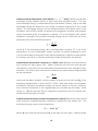
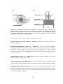
VAMPIRE
User Manual
VAMPIRE
User Manual
Software version 4.0
Manual written by Richard F. L. Evans and Andreas Biternas.
Copyright © 2014 Department of Physics, The University of York, Heslington, York,
YO10 5DD. All rights Reserved.
The VAMPIRE software package is principally developed and maintained by Richard
F. L. Evans. Code contributors: Weijia Fan, Phanwadee Chureemart, Thomas Ostler,
Joe Barker, Andreas Biternas and Roy Chantrell.
The entire VAMPIRE package is available under the GNU General Public License.
You are free to use vampire for personal, academic and commercial research, and
to modify the source code as you wish. For details of the licence, check the README
file in the source code or consult www.gnu.org/copyleft/gpl.html.
The VAMPIRE source code is available from www.github.com/richard-evans/vampire.
This manual, software features, tutorials and more information is available from the
VAMPIRE webpage at http://vampire.york.ac.uk/
1
Table of Contents
Table of Contents
2
Preface
9
Introducing VAMPIRE . . . . . . . . . . . . . . . . . . . . . . . . . . . . . .
1 Background theory
9
10
Atomistic Spin Models . . . . . . . . . . . . . . . . . . . . . . . . . . . . . 10
The spin Hamiltonian . . . . . . . . . . . . . . . . . . . . . . . . . . . . . . 11
Spin Dynamics . . . . . . . . . . . . . . . . . . . . . . . . . . . . . . . . . 11
Citations . . . . . . . . . . . . . . . . . . . . . . . . . . . . . . . . . . . . . 12
2 Installation
13
System Requirements . . . . . . . . . . . . . . . . . . . . . . . . . . . . . . 13
Binary installation . . . . . . . . . . . . . . . . . . . . . . . . . . . . . . . . 13
Compiling from source . . . . . . . . . . . . . . . . . . . . . . . . . . . . . 14
Compiling on Linux . . . . . . . . . . . . . . . . . . . . . . . . . . . . 14
Compiling on Mac OSX . . . . . . . . . . . . . . . . . . . . . . . . . . 14
Compiling on Windows . . . . . . . . . . . . . . . . . . . . . . . . . . 14
3 Running the code
16
Running on Linux and Mac OS X . . . . . . . . . . . . . . . . . . . . . . . . 16
Running on Windows . . . . . . . . . . . . . . . . . . . . . . . . . . . . . . 16
Serial version . . . . . . . . . . . . . . . . . . . . . . . . . . . . . . . 16
Parallel version (1 PC) . . . . . . . . . . . . . . . . . . . . . . . . . . . 16
Parallel version (2+ PCs) . . . . . . . . . . . . . . . . . . . . . . . . . 17
4 Getting Started
19
Feature Overview . . . . . . . . . . . . . . . . . . . . . . . . . . . . . . . . 19
Input and Output Files . . . . . . . . . . . . . . . . . . . . . . . . . . . . . 20
Sample input files . . . . . . . . . . . . . . . . . . . . . . . . . . . . . . . . 20
2
5 Input File Command Reference
22
System Generation . . . . . . . . . . . . . . . . . . . . . . . . . . . . . . . 22
create:full . . . . . . . . . . . . . . . . . . . . . . . . . . . . . . . . . 22
create:cube . . . . . . . . . . . . . . . . . . . . . . . . . . . . . . . . 22
create:cylinder . . . . . . . . . . . . . . . . . . . . . . . . . . . . . . . 22
create:ellipsoid . . . . . . . . . . . . . . . . . . . . . . . . . . . . . . 22
create:sphere . . . . . . . . . . . . . . . . . . . . . . . . . . . . . . . 22
create:truncated-octahedron . . . . . . . . . . . . . . . . . . . . . . . 22
create:particle . . . . . . . . . . . . . . . . . . . . . . . . . . . . . . . 23
create:particle-array . . . . . . . . . . . . . . . . . . . . . . . . . . . . 23
create:voronoi-film . . . . . . . . . . . . . . . . . . . . . . . . . . . . . 23
create:voronoi-size-variance . . . . . . . . . . . . . . . . . . . . . . . 23
create:voronoi-row-offset . . . . . . . . . . . . . . . . . . . . . . . . . 23
create:voronoi-random-seed . . . . . . . . . . . . . . . . . . . . . . . 23
create:voronoi-rounded-grains . . . . . . . . . . . . . . . . . . . . . . 24
create:voronoi-rounded-grains-area . . . . . . . . . . . . . . . . . . . 24
create:particle-parity . . . . . . . . . . . . . . . . . . . . . . . . . . . 24
create:crystal-structure . . . . . . . . . . . . . . . . . . . . . . . . . . 24
create:single-spin . . . . . . . . . . . . . . . . . . . . . . . . . . . . . 24
create:periodic-boundaries-x . . . . . . . . . . . . . . . . . . . . . . . 24
create:periodic-boundaries-y . . . . . . . . . . . . . . . . . . . . . . . 24
create:periodic-boundaries-z . . . . . . . . . . . . . . . . . . . . . . . 24
create:select-material-by-height . . . . . . . . . . . . . . . . . . . . . 24
create:select-material-by-geometry
. . . . . . . . . . . . . . . . . . . 24
create:fill-core-shell-particles . . . . . . . . . . . . . . . . . . . . . . . 24
create:interfacial-roughness . . . . . . . . . . . . . . . . . . . . . . . 24
create:material-interfacial-roughness . . . . . . . . . . . . . . . . . . . 25
create:interfacial-roughness-random-seed . . . . . . . . . . . . . . . . 25
create:interfacial-roughness-number-of-seed-points . . . . . . . . . . 25
create:interfacial-roughness-type . . . . . . . . . . . . . . . . . . . . . 25
create:interfacial-roughness-seed-radius . . . . . . . . . . . . . . . . 25
create:interfacial-roughness-seed-radius-variance . . . . . . . . . . . 25
create:interfacial-roughness-mean-height . . . . . . . . . . . . . . . . 25
create:interfacial-roughness-maximum-height . . . . . . . . . . . . . . 25
create:interfacial-roughness-height-field-resolution . . . . . . . . . . . 25
System dimensions . . . . . . . . . . . . . . . . . . . . . . . . . . . . . . . 25
dimensions:unit-cell-size . . . . . . . . . . . . . . . . . . . . . . . . . 25
dimensions:unit-cell-size-x . . . . . . . . . . . . . . . . . . . . . . . . 25
3
dimensions:unit-cell-size-y . . . . . . . . . . . . . . . . . . . . . . . . 25
dimensions:unit-cell-size-z . . . . . . . . . . . . . . . . . . . . . . . . 25
dimensions:system-size . . . . . . . . . . . . . . . . . . . . . . . . . . 25
dimensions:system-size-x . . . . . . . . . . . . . . . . . . . . . . . . . 25
dimensions:system-size-y . . . . . . . . . . . . . . . . . . . . . . . . . 25
dimensions:system-size-z . . . . . . . . . . . . . . . . . . . . . . . . . 26
dimensions:particle-size
. . . . . . . . . . . . . . . . . . . . . . . . . 26
dimensions:particle-spacing . . . . . . . . . . . . . . . . . . . . . . . 26
dimensions:particle-shape-factor-z . . . . . . . . . . . . . . . . . . . . 26
dimensions:particle-shape-factor-y . . . . . . . . . . . . . . . . . . . . 26
dimensions:particle-shape-factor-z . . . . . . . . . . . . . . . . . . . . 26
dimensions:particle-array-offset-x . . . . . . . . . . . . . . . . . . . . 26
dimensions:particle-array-offset-y . . . . . . . . . . . . . . . . . . . . 26
dimensions:macro-cell-size . . . . . . . . . . . . . . . . . . . . . . . . 26
Simulation Control . . . . . . . . . . . . . . . . . . . . . . . . . . . . . . . . 26
sim:integrator . . . . . . . . . . . . . . . . . . . . . . . . . . . . . . . 26
sim:program . . . . . . . . . . . . . . . . . . . . . . . . . . . . . . . . 27
sim:enable-dipole-fields . . . . . . . . . . . . . . . . . . . . . . . . . . 28
sim:enable-fmr-field . . . . . . . . . . . . . . . . . . . . . . . . . . . . 28
sim:enable-fast-dipole-fields . . . . . . . . . . . . . . . . . . . . . . . 28
sim:dipole-field-update-rate
. . . . . . . . . . . . . . . . . . . . . . . 28
sim:enable-surface-anisotropy . . . . . . . . . . . . . . . . . . . . . . 28
sim:surface-anisotropy-threshold . . . . . . . . . . . . . . . . . . . . . 28
sim:surface-anisotropy-nearest-neighbour-range . . . . . . . . . . . . 28
sim:time-step . . . . . . . . . . . . . . . . . . . . . . . . . . . . . . . 29
sim:total-time-steps . . . . . . . . . . . . . . . . . . . . . . . . . . . . 29
sim:loop-time-steps . . . . . . . . . . . . . . . . . . . . . . . . . . . . 29
sim:time-steps-increment . . . . . . . . . . . . . . . . . . . . . . . . . 29
sim:equilibration-time-steps . . . . . . . . . . . . . . . . . . . . . . . . 29
sim:simulation-cycles . . . . . . . . . . . . . . . . . . . . . . . . . . . 29
sim:maximum-temperature . . . . . . . . . . . . . . . . . . . . . . . . 29
sim:minimum-temperature . . . . . . . . . . . . . . . . . . . . . . . . 29
sim:equilibration-temperature . . . . . . . . . . . . . . . . . . . . . . . 29
sim:temperature . . . . . . . . . . . . . . . . . . . . . . . . . . . . . . 29
sim:temperature-increment . . . . . . . . . . . . . . . . . . . . . . . . 29
sim:cooling-time . . . . . . . . . . . . . . . . . . . . . . . . . . . . . . 29
sim:laser-pulse-temporal-profile . . . . . . . . . . . . . . . . . . . . . 29
sim:laser-pulse-time . . . . . . . . . . . . . . . . . . . . . . . . . . . . 29
4
sim:laser-pulse-power . . . . . . . . . . . . . . . . . . . . . . . . . . . 29
sim:second-laser-pulse-time . . . . . . . . . . . . . . . . . . . . . . . 29
sim:second-laser-pulse-power . . . . . . . . . . . . . . . . . . . . . . 29
sim:second-laser-pulse-maximum-temperature . . . . . . . . . . . . . 29
sim:second-laser-pulse-delay-time . . . . . . . . . . . . . . . . . . . . 30
sim:two-temperature-heat-sink-coupling . . . . . . . . . . . . . . . . . 30
sim:two-temperature-electron-heat-capacity . . . . . . . . . . . . . . . 30
sim:two-temperature-phonon-heat-capacity . . . . . . . . . . . . . . . 30
sim:two-temperature-electron-phonon-coupling . . . . . . . . . . . . . 30
sim:cooling-function . . . . . . . . . . . . . . . . . . . . . . . . . . . . 30
sim:applied-field-strength . . . . . . . . . . . . . . . . . . . . . . . . . 30
sim:maximum-applied-field-strength . . . . . . . . . . . . . . . . . . . 30
sim:equilibration-applied-field-strength
. . . . . . . . . . . . . . . . . 30
sim:applied-field-strength-increment . . . . . . . . . . . . . . . . . . . 30
sim:applied-field-angle-theta . . . . . . . . . . . . . . . . . . . . . . . 30
sim:applied-field-angle-phi . . . . . . . . . . . . . . . . . . . . . . . . 30
sim:applied-field-unit-vector . . . . . . . . . . . . . . . . . . . . . . . 30
sim:demagnetisation-factor . . . . . . . . . . . . . . . . . . . . . . . . 30
sim:mpi-mode . . . . . . . . . . . . . . . . . . . . . . . . . . . . . . . 31
sim:integrator-random-seed
. . . . . . . . . . . . . . . . . . . . . . . 31
sim:constraint-rotation-update . . . . . . . . . . . . . . . . . . . . . . 31
sim:constraint-angle-theta
. . . . . . . . . . . . . . . . . . . . . . . . 31
sim:constraint-angle-theta-minimum . . . . . . . . . . . . . . . . . . . 31
sim:constraint-angle-theta-maximum . . . . . . . . . . . . . . . . . . . 31
sim:constraint-angle-theta-increment . . . . . . . . . . . . . . . . . . . 31
sim:constraint-angle-phi
. . . . . . . . . . . . . . . . . . . . . . . . . 31
sim:constraint-angle-phi-minimum . . . . . . . . . . . . . . . . . . . . 31
sim:constraint-angle-phi-maximum . . . . . . . . . . . . . . . . . . . . 31
sim:constraint-angle-phi-increment . . . . . . . . . . . . . . . . . . . . 31
sim:monte-carlo-algorithm . . . . . . . . . . . . . . . . . . . . . . . . 31
sim:checkpoint
. . . . . . . . . . . . . . . . . . . . . . . . . . . . . . 31
Data output . . . . . . . . . . . . . . . . . . . . . . . . . . . . . . . . . . . 32
output:time-steps . . . . . . . . . . . . . . . . . . . . . . . . . . . . . 32
output:real-time . . . . . . . . . . . . . . . . . . . . . . . . . . . . . . 32
output:temperature . . . . . . . . . . . . . . . . . . . . . . . . . . . . 32
output:applied-field-strength . . . . . . . . . . . . . . . . . . . . . . . 32
output:applied-field-unit-vector . . . . . . . . . . . . . . . . . . . . . . 32
output:applied-field-alignment . . . . . . . . . . . . . . . . . . . . . . 32
5
output:material-applied-field-alignment . . . . . . . . . . . . . . . . . 32
output:magnetisation . . . . . . . . . . . . . . . . . . . . . . . . . . . 32
output:magnetisation-length . . . . . . . . . . . . . . . . . . . . . . . 32
output:mean-magnetisation-length . . . . . . . . . . . . . . . . . . . . 33
output:material-magnetisation . . . . . . . . . . . . . . . . . . . . . . 33
output:material-mean-magnetisation-length . . . . . . . . . . . . . . . 33
output:total-torque . . . . . . . . . . . . . . . . . . . . . . . . . . . . . 33
output:mean-total-torque . . . . . . . . . . . . . . . . . . . . . . . . . 33
output:constraint-phi
. . . . . . . . . . . . . . . . . . . . . . . . . . . 33
output:constraint-theta . . . . . . . . . . . . . . . . . . . . . . . . . . 33
output:material-mean-torque . . . . . . . . . . . . . . . . . . . . . . . 34
output:mean-susceptibility . . . . . . . . . . . . . . . . . . . . . . . . 34
output:electron-temperature . . . . . . . . . . . . . . . . . . . . . . . 34
output:phonon-temperature . . . . . . . . . . . . . . . . . . . . . . . . 34
output:total-energy . . . . . . . . . . . . . . . . . . . . . . . . . . . . 34
output:mean-total-energy . . . . . . . . . . . . . . . . . . . . . . . . . 34
output:anisotropy-energy . . . . . . . . . . . . . . . . . . . . . . . . . 34
output:mean-anisotropy-energy
. . . . . . . . . . . . . . . . . . . . . 34
output:cubic-anisotropy-energy
. . . . . . . . . . . . . . . . . . . . . 35
output:mean-cubic-anisotropy-energy . . . . . . . . . . . . . . . . . . 35
output:surface-anisotropy-energy
. . . . . . . . . . . . . . . . . . . . 35
output:mean-surface-anisotropy-energy . . . . . . . . . . . . . . . . . 35
output:exchange-energy . . . . . . . . . . . . . . . . . . . . . . . . . 35
output:mean-exchange-energy . . . . . . . . . . . . . . . . . . . . . . 35
output:applied-field-energy . . . . . . . . . . . . . . . . . . . . . . . . 35
output:mean-applied-field-energy . . . . . . . . . . . . . . . . . . . . 35
output:magnetostatic-energy . . . . . . . . . . . . . . . . . . . . . . . 35
output:mean-magnetostatic-energy . . . . . . . . . . . . . . . . . . . 35
output:second-order-uniaxial-anisotropy-energy
. . . . . . . . . . . . 35
output:mean-second-order-uniaxial-anisotropy-energy . . . . . . . . . 35
output:mpi-timings . . . . . . . . . . . . . . . . . . . . . . . . . . . . . 35
output:gnuplot-array-format . . . . . . . . . . . . . . . . . . . . . . . . 35
output:output-rate . . . . . . . . . . . . . . . . . . . . . . . . . . . . . 35
Configuration output . . . . . . . . . . . . . . . . . . . . . . . . . . . . . . 36
config:atoms . . . . . . . . . . . . . . . . . . . . . . . . . . . . . . . . 36
config:atoms-output-rate . . . . . . . . . . . . . . . . . . . . . . . . . 36
config:atoms-min-x . . . . . . . . . . . . . . . . . . . . . . . . . . . . 36
config:atoms-min-y . . . . . . . . . . . . . . . . . . . . . . . . . . . . 36
6
config:atoms-min-z . . . . . . . . . . . . . . . . . . . . . . . . . . . . 36
config:atoms-max-x . . . . . . . . . . . . . . . . . . . . . . . . . . . . 36
config:atoms-max-y . . . . . . . . . . . . . . . . . . . . . . . . . . . . 36
config:atoms-max-z . . . . . . . . . . . . . . . . . . . . . . . . . . . . 36
config:macro-cells . . . . . . . . . . . . . . . . . . . . . . . . . . . . . 36
config:macro-cells-output-rate . . . . . . . . . . . . . . . . . . . . . . 36
config:identify-surface-atoms . . . . . . . . . . . . . . . . . . . . . . . 36
6 Material File Command Reference
37
material:num-materials . . . . . . . . . . . . . . . . . . . . . . . . . . 37
material:material-name . . . . . . . . . . . . . . . . . . . . . . . . . . 37
material:damping-constant . . . . . . . . . . . . . . . . . . . . . . . . 37
material:exchange-matrix . . . . . . . . . . . . . . . . . . . . . . . . . 38
material:atomic-spin-moment . . . . . . . . . . . . . . . . . . . . . . . 38
material:uniaxial-anisotropy-constant . . . . . . . . . . . . . . . . . . . 38
material:second-uniaxial-anisotropy-constant . . . . . . . . . . . . . . 39
material:cubic-anisotropy-constant . . . . . . . . . . . . . . . . . . . . 39
material:uniaxial-anisotropy-direction
. . . . . . . . . . . . . . . . . . 39
material:surface-anisotropy-constant . . . . . . . . . . . . . . . . . . . 39
material:relative-gamma
. . . . . . . . . . . . . . . . . . . . . . . . . 40
material:initial-spin-direction . . . . . . . . . . . . . . . . . . . . . . . 40
material:material-element . . . . . . . . . . . . . . . . . . . . . . . . . 40
material:geometry-file . . . . . . . . . . . . . . . . . . . . . . . . . . . 40
material:alloy-host . . . . . . . . . . . . . . . . . . . . . . . . . . . . . 40
material:alloy-fraction . . . . . . . . . . . . . . . . . . . . . . . . . . . 41
material:minimum-height . . . . . . . . . . . . . . . . . . . . . . . . . 41
material:maximum-height . . . . . . . . . . . . . . . . . . . . . . . . . 41
material:core-shell-size . . . . . . . . . . . . . . . . . . . . . . . . . . 41
material:interface-roughness . . . . . . . . . . . . . . . . . . . . . . . 42
material:intermixing . . . . . . . . . . . . . . . . . . . . . . . . . . . . 42
material:density . . . . . . . . . . . . . . . . . . . . . . . . . . . . . . 42
material:continuous . . . . . . . . . . . . . . . . . . . . . . . . . . . . 42
material:fill-space . . . . . . . . . . . . . . . . . . . . . . . . . . . . . 42
material:couple-to-phononic-temperature . . . . . . . . . . . . . . . . 43
material:temperature-rescaling-exponent . . . . . . . . . . . . . . . . 43
material:temperature-rescaling-curie-temperature . . . . . . . . . . . . 43
Example material files . . . . . . . . . . . . . . . . . . . . . . . . . . . . . . 43
7
Bibliography
44
8
Introducing VAMPIRE
VAMPIRE is a state-of-the-art atomistic simulator for magnetic nanomaterials. This
software is the culmination of five years of continuous development, with an aim
to make atomistic simulation of magnetic materials routinely available to the nonspecialist researcher. Before now, using atomistic models to simulate magnetic
systems required in depth and technical knowledge of the underlying theoretical
methods, computer programming skills and the ability to debug and understand
intricate computational problems. The code is designed with ease of use in mind,
and includes an extensive set of input parameters to control the simulations through
a plain text input file. Subject to future funding it is also hoped to develop graphical
user interfaces for MacTM OS X and WindowsTM which should make using the code
more accessible.
The VAMPIRE project is still very much under active development, and a yearly
release schedule in the Autumn is planned to make the latest improvements available
for everyone. These features are always available during the development stages
from the develop branch of the code, but with the caveat that they are not always
fully reliable. Feedback of any bugs or errors to the VAMPIRE developers is always
welcome, as well as any feature requests or enhancements.
We hope that as the VAMPIRE project develops it will become a useful tool for the
magnetics community for specialists and non-specialists alike.
9
1
Background theory
While the underlying theory behind the atomistic spin model is well known in the
scientific literature, in the following a very brief overview of the fundamental theory
is presented for the benefit of those who do not wish to study the methods in great
detail. If more information is required then a comprehensive review of the methods
implemented in VAMPIRE is available from the project website.
Atomistic Spin Models
Atomistic spin models form the natural limit of two distinct approaches, namely
micromagnetics and ab-initio models of the electronic structure. In micromagnetics a
material is discretized into small domains where the magnetization is assumed to be
fully ordered within. If the micromagnetic cell size is reduced to less than 1 nm, then
the magnetization is no longer a true continuum, but a discrete entity considering
localized moments on individual atoms. Similarly, when the electronic properties
of the system are considered, the quantum mechanical properties can be mapped
onto atomic cores in a manner similar to molecular dynamics, where the effective
properties can often be treated in a classical approximation.
The advantage of the atomistic model over micromagnetics is that it naturally
deals with atomic ordering and variation of local properties seen in real materials,
such as interfaces, defects, roughness etc. The discrete formulation also allows the
simulation of high temperatures above and beyond the Curie temperature, where
the usual continuum micromagnetic approach breaks down. Such effects or often
central to current problems in magnetism such as materials for spin electronics,
heat assisted magnetic recording or ultrafast laser processes. Similarly for ab-initio
calculations, mapping onto an effective spin model allows apply the full quantum
mechanical deal of the properties to much larger systems and the consideration of
dynamic effects on much longer timescales.
10
The Spin Hamiltonian
The basis of the atomistic spin model is the spin Hamiltonian, which describes the
fundamental spin-dependent interactions at the atomic level (neglecting the effects
of potential and kinetic energy and electron correlations). The spin Hamiltonian is
typically defined as
H =−
∑
Jij Si · Sj − k2
∑
i,j
i
S2z − μ S
∑
Happ · Si
i
describing exchange, uniaxial anisotropy and applied field contributions respectively. Important parameters are the Heisenberg exchange Jij , the anisotropy
constant k2 and the atomic spin moment, μ S . Si is a unit vector which describes
the orientation of the local spin moment. In most magnetic materials the exchange
interactions are the dominant contribution, usually by two orders of magnitude, and
gives rise to the atomic ordering of the spin directions. For ferromagnetic materials
(parallel alignment of spins) Jij > 0, while for anti-ferromagnetic materials (antiparallel
alignment of spins), Jij < 0.
While the exchange interaction determines the ordering of the spins, it is usually
isotropic, and so there is no preferential orientation of all the spins in the system. Most
magnetic materials are anisotropic, that is the spins have a preferred orientation in
space, which arises at the atomic level due to the local crystal environment, hence
its full name of magnetocrystalline anisotropy. In the model this is most commonly
uniaxial anisotropy, where the spins prefer to lie along a single preferred axis, known
as the easy axis. The strength of the anisotropy is determined by the anisotropy
constant, in our case k2 , where positive value prefer alignment along the z-axis, while
negative values prefer alignment around the x − y plane.
The last term describes the coupling of the spin system to an externally applied
field, Happ , or Zeeman field. The applied field is used to reverse the orientation of the
spins, and can be used in the simulation to calculate hysteresis loops, for example.
Spin Dynamics
The spin Hamiltonian describes the energetics of the system, but says nothing about
the dynamic behaviour. For that the Landau-Lifshitz-Gilbert (LLG) equation is used
to describe the dynamics of atomic spins. The LLG is given by
γ
∂ Si
=−
[Si × Hieff + λSi × (Si × Hieff )]
∂t
(1 + λ2 )
11
(1.1)
where Si is a unit vector representing the direction of the magnetic spin moment of
site i, γ is the gyromagnetic ratio and Hieff is the net magnetic field on each spin. The
atomistic LLG equation describes the interaction of an atomic spin moment i with an
effective magnetic field, which is obtained from the negative first derivative of the
complete spin Hamiltonian, such that:
Hieff = −
1 ∂H
μ S ∂ Si
(1.2)
where μ S is the local spin moment. The inclusion of the spin moment within the
effective field is significant, in that the field is then expressed in units of Tesla, given
a Hamiltonian in Joules. The LLG is integrated numerically using the Heun numerical
scheme, which allows the time evolution of the spin system to be simulated.
Citations
If you use VAMPIRE for your research, please cite the following article:
Atomistic spin model simulations of magnetic nanomaterials
R. F. L. Evans, W. J. Fan, P. Chureemart, T. A. Ostler, M. O. A. Ellis and R. W. Chantrell
J. Phys.: Condens. Matter 26, 103202 (2014)
If you use the constrained Monte Carlo method, in addition please cite:
Constrained Monte Carlo method and calculation of the temperature dependence of magnetic
anisotropy
P. Asselin, R. F. L. Evans, J. Barker, R. W. Chantrell, R. Yanes, O. Chubykalo-Fesenko, D. Hinzke
and U. Nowak
Phys. Rev. B. 82, 054415 (2010)
If you use the temperature rescaling method please cite:
Quantitative simulation of temperature-dependent magnetization dynamics and equilibrium properties of elemental ferromagnets
R. F. L. Evans, U. Atxitia, and R. W. Chantrell
Phys. Rev. B 91, 144425 (2015)
12
2
Installation
This chapter covers the requirements, installation and support for VAMPIRE on
different platforms.
System Requirements
VAMPIRE is designed to be generally portable and compilable on Linux, Unix, Mac
OSX and Windows with a range of different compilers. By design the software has
a very minimal dependence on external libraries to aid compilation on the widest
possible range of platforms without needing to first install and configure a large
number of other packages. VAMPIRE is designed to be maximally efficient on high
performance computing clusters and scalable to thousands of processors, and as
such is the recommended platform if you have access to appropriate resources.
Hardware Requirements
VAMPIRE has been successfully tested on a wide variety of x86 and power PC
processors. Memory requirements are generally relatively modest for most systems,
though larger simulations will require significantly more memory. VAMPIRE is generally
computationally limited, and so the faster the clock speed and number of processor
cores the better.
Binary installation
Compiled binaries of the latest release version are available to download from:
http://vampire.york.ac.uk/download/
for Linux, MacTM OS X and WindowsTM platforms. For the Linux and Mac OS X
releases, a simple installation script install.sh installs the binary in /opt/vampire/ and
appends the directory to your environment path. The Windows binary is redistributable, and must simply be in the same directory as the input file, however, before
running the code you need to install the Microsoft Visual C++ 2008 Redistributable
(see the next chapter on running VAMPIRE). From version 4.0 onwards a copy of
13
qvoronoi is integrated into VAMPIRE for generating granular structures.
Compiling from source
The best way to get the vampire source code is using git, a distributed version control
program which enables changes in the code to be tracked. Git is readily available
on linux (git-core package on ubuntu) and Mac (via MacPorts). To get vampire from
the Github repository checkout your own copy of the repository using:
git clone git://github.com/richard-evans/vampire.git
This way, updates to the code can be easily merged with the downloaded version.
Compiling is generally as easy as running make in Unix platforms.
Compiling on Linux
In order to compile in linux, a working set of development tools are needed, which
on ubuntu includes the packages build-essential and g++. VAMPIRE should compile
without issue following a simple make command in the source directory.
For the parallel version, a working installation of openmpi is recommended, which
must usually include a version of the development tools (openmpi-bin and openmpidev packages on ubuntu). Compilation is usually straightforward using make parallel.
Compiling on Mac OSX
With OS X, compilation from source requires a working installation of Xcode, available
for free from the Mac App Store. In addition command line tools must also be
installed. A working installation of MacPorts is recommended to provide access to a
wide range of open source libraries and tools such as openmpi, rasmol and povray.
For the serial version, compilation is the same as for linux, following a simple make
command in the source directory.
Similarly for the parallel version, openmpi needs to be installed via MacPorts, and
compilation is usually straightforward using make parallel.
Compiling on Windows
In order to compile the code on Windows systems you will need to have Microsoft
Visual Studio 2010 or later and open the file Vampire.vcxproj with it. The project has
two versions: Debug and Release, where you can choose the current one in the dropdown menu on the top toolbar. The first is for debugging the code and the executable
which is created will not be a stand-alone executable. The Release version is for
creating a stand-alone executables for the serial version. Click Build>Project to
14
compile the code.
Finally, you can compile a 64-bit version if you choose from the drop down menu
in the top toolbar in MS Visual Studio. (It writes “Win32” so when you click it the x64
option will appear).
15
3
Running the code
To run the code in all version, you first need to specify an input file and material file,
which must reside in the same directory where you run the code. Example files are
available in the source code distribution, or from the Download section of the website
(http://vampire.york.ac.uk/download/index.html).
Linux Debian/Ubuntu and Mac OS X
In the directory including the input and material files, typing ./vampire will run the
code in serial mode. For the parallel mode with openmpi, mpirun -np 2 vampire will
run the code in parallel mode, on 2 CPUs. Increasing the -np argument will run on
more cores.
Windows
In order to run any Windows version of VAMPIRE, you need to have “Microsoft Visual
C++ 2008 Redistributable” library or newer installed on your PC. Usually this is
installed by default, but if the executable fails to run then download and install it
from here:
http://www.microsoft.com/en-gb/download/details.aspx?id=29
Serial version
The serial version can be run by double clicking the executable file, where the
executable, input and material files are in the same directory. You may also want
to run the code using the command line in case there are error messages. In this
case you should change to the directory containing the input files and executables
using the usual cd commands. VAMPIRE can then be run by simply typing ‘vampire’.
Parallel version using MPICH2 (1 PC)
The parallel version of VAMPIRE requires a working installation of MPICH2 which must
be installed as follows.
16
Set up MPICH2
• Download and install MPICH2 from:
http://www.mpich.org/static/tarballs/1.4.1p1/mpich2-1.4.1p1-win-ia32.msi
• Put its bin directory to the path. This is how to do that:
– Right Click “My Computer” and then Properties.
– Click on left the “Advanced system settings”
– On the “Advanced” tab click the Environment Variables at the bottom
– In the “System Variables” list at the bottom scroll down to find the “Path”
variable. Select it and click “Edit”.
– Go to the end of “Variable value:” and write “;Mpich2path/bin” where
Mpich2path is the path where you install your Mpich2. The “;” put it if
does not exist before. So e.g. what I have in my pc is “C:\Program Files
(x86)\MPICH2\bin”.
• Open a Command Prompt and write:
smpd -install
mpiexec -remove
mpiexec -register ,where give as username the exact username for login
in the windows and password your exact password for login windows.
smpd -install
Run the code
To run the parallel version it is necessary to launch the code with the mpiexec
command. To do this, first open the MSDOS prompt. Navigate to the directory
containing the binary and execute the following command:
mpiexec -n number_of_processors Vampire-Parallel.exe
replacing number_of_processors with the number of processors/cores you want
to use in this system (e.g.: mpiexec -n 4 Vampire-Parallel.exe for a quad core
machine).
Parallel version using MPICH2 (2+ PCs)
For multiple PCs in addition to a working MPICH2 implementation, you must also
setup the PCs shared folder and firewall as detailed below.
17
Configure MPICH2 for multiple PCs
• For every PC install MPICH2 as detailed in the last section.
• Only for the running PC: Right click the folder where Vampire-Parallel.exe. is
and click “Properties”, go to “Sharing Tab” and click “Share”. Then, if your
name is there OK else choose your name from dropdown menu and click
“Add” . In the permission level choose to be Read/write next to your name.
• Every PC: Put the files C:\Program Files (x86)\MPICH2\bin\smpd.exe , C:\Program
Files (x86)\MPICH2\bin\mpiexec.exe and Vampire-Parallel.exe in the exception list of Windows Firewall(maybe there already in this list):
– Bring up the windows firewall from the control panel
– Click on “Allow a program or feature through Windows Firewall”, click
“Change settings” and click “Allow another program” and Browse. Go
to find these files in their directories, and the Vampire-Parallel.exe go in
the Network, then to the running PC and then to the folder.
• (Optional) Only for the running PC: In order to make the log files to join and the
program finish as expected you must do that: Run regedit and find the key
HKEY_CURRENT_USER\Software\Microsoft\Command Processor and click
add DWORD with the name DisableUNCCheck and give it value 1 (will appear
o 0 x 1 (Hex)).
Run the code
To run VAMPIRE on multiple machine execute the following command:
mpiexec -hosts number_of_hosts PC1 np1 PC2 np2
-dir \\PC1\Vampire\\\PC1\Vampire\Vampire-Parallel.exe
number_of_hosts
PC1
np1
PC2
np2
\\PC1\Vampire\
number of PCs you want to use
name of the 1st PC
number of cores to use in PC1
name of the 2nd PC
number of cores to use in PC2
shared directory where all the PCs
can find the executable and input
files
the executable location
\\PC1\Vampire\Vampire-Parallel.exe
18
4
Getting Started
VAMPIRE is a powerful software package, capable of simulating many different
systems and the determination of parameters such as coercivity, Curie points,
reversal dynamics, statistical behaviour and more. This chapter contains an overview
of the capabilities of VAMPIRE and how to use them.
Feature Overview
The features of VAMPIRE are split into three main categories: material parameters,
structural parameters, and simulation parameters. Details of these parameters are
given in the following chapters, but between them they define the parameters for a
particular simulation.
Materials
Material parameters essentially define the magnetic properties of a class of atoms,
including magnetic moments, exchange interactions, damping constants etc. VAMPIRE includes support for up to one hundred defined materials, and material parameters control the simulation of multilayers, random alloys, core shell particles and
lithographically defined patterns.
Structures
Structural parameters define properties such as the system size, shape, particle size,
or voronoi grain structures. In combination with material parameters they essentially
define the system to be simulated.
Simulations
VAMPIRE includes a number of built-in simulations for determining the most common
magnetic properties of a system Ð for example Curie temperature, hysteresis loops,
or even a time series. Additionally the parameters for these simulations, such as
applied field, maximum temperature, temperature increment, etc. can be set.
19
Input and Output Files
VAMPIRE requires at least two files to run a simulation, the input file and the material
file. The input file defines all the properties of the simulated system, such as the
dimensions or particle shape, as well as the simulation parameters and program
output. The material file defines the properties of all the materials used in the
simulation, and is usually given the .mat file extension. A sample material file Co.mat
is included with the code which defines a minimum set of parameters for Co.
The output of the code includes a main output file, which records data such as
the magnetisation, timesteps, temperature etc. The format of the output file is fully
customisable, so that the amount of output data is limited to what is useful. In addition
to the output file, the other main available output are spin configuration files, which
with post-processing allow output of snapshots of the magnetic configurations during
the simulation.
Sample input files
Sample input and output files are included in the source code distribution, but
the files for a simple test simulation which computes the time dependence of the
magnetisation of a cubic system are given here.
input
#-----------------------------------------# Sample vampire input file to perform
# benchmark calculation for v4.0
#
#-----------------------------------------#-----------------------------------------# Creation attributes:
#-----------------------------------------create:crystal-structure=sc
#-----------------------------------------# System Dimensions:
#-----------------------------------------dimensions:unit-cell-size = 3.54 !A
dimensions:system-size-x = 7.7 !nm
dimensions:system-size-y = 7.7 !nm
dimensions:system-size-z = 7.7 !nm
#-----------------------------------------# Material Files:
#-----------------------------------------material:file="Co.mat"
20
#-----------------------------------------# Simulation attributes:
#-----------------------------------------sim:temperature=300.0
sim:time-steps-increment=1000
sim:total-time-steps=10000
sim:time-step=1.0E-15
#-----------------------------------------# Program and integrator details
#-----------------------------------------sim:program=benchmark
sim:integrator=llg-heun
#-----------------------------------------# data output
#-----------------------------------------output:real-time
output:temperature
output:magnetisation
output:magnetisation-length
screen:time-steps
screen:magnetisation-length
Co.mat
#===================================================
# Sample vampire material file V4+
#===================================================
#--------------------------------------------------# Number of Materials
#--------------------------------------------------material:num-materials=1
#--------------------------------------------------# Material 1 Cobalt Generic
#--------------------------------------------------material[1]:material-name="Co"
material[1]:damping-constant=1.0
material[1]:exchange-matrix[1]=11.2e-21
material[1]:atomic-spin-moment=1.72 !muB
material[1]:uniaxial-anisotropy-constant=1.0e-24
material[1]:material-element="Ag"
material[1]:minimum-height=0.0
material[1]:maximum-height=1.0
21
5
Input File Command Reference
The input file can accept a large number of commands, and this chapter gives a
comprehensive list of all the options and what they do. Commands are in the form
category :keyword=value, where value can be optional depending on the keyword.
System Generation
The following commands control generation of the simulated system, including
dimensions, crystal structures etc.
create:full Uses the entire generated system without any truncation or consideration
of the create:particle-size parameter. create:full should be used when importing a
complete system, such as a complete nanoparticle and where a further definition of
the system shape is not required. This is the default if no system truncation is defined.
create:cube Cuts a cuboid particle of size lx = ly = lz = create:particle-size from the
defined crystal lattice.
create:cylinder Cuts a cylindrical particle of diameter create:particle-size from the
defined crystal lattice. The height of the cylinder extends to the whole extent of the
system size create:system-size-z in the z-direction.
create:ellipsoid Cuts an ellipsoid particle of diameter create:particle-size with frac-
tional diameters of dimensions:particle-shape-factor-x,dimensions:particle-shape-factory,dimensions:particle-shape-factor-z from the defined crystal lattice.
create:sphere Cuts a spherical particle of diameter create:particle-size from the
defined crystal lattice.
create:truncated-octahedron Cuts a truncated octahedron particle of diameter create:particle-
size from the defined crystal lattice.
22
create:particle Defines the creation of a single particle at the centre of the defined
system. If create:particle-size is greater than the system dimensions then the outer
boundary of the particle is truncated by the system dimensions.
create:particle-array Defines the creation of a two-dimensional array of particles on
a square lattice. The particles are separated by a distance create:particle-spacing.
If the system size is insufficient to contain at least a single entire particle of size
create:particle-size then no atoms will be generated and the program will terminate
with an error.
create:voronoi-film Generates a two-dimensional voronoi structure of particles, with a
mean grain size of create:particle-size and variance create:voronoi-size-variance as
a fraction of the grain size. If create:voronoi-size-variance=0 then hexagonal shaped
grains are generated. The spacing between the grains (defined by the initial voronoi
seed points) is controlled by create:particle-spacing. The pseudo-random pattern
uses a predefined random seed, and so the generated structure will be the same
every time. A different structure can be generated by setting a new random seed
using the create:voronoi-random-seed parameter. Depending on the desired edge
structure, the first row can be shifted using the create:voronoi-row-offset flag which
changes the start point of the voronoi pattern. The create:voronoi-rounded-grains
parameter generates a voronoi structure, but then applies a grain rounding algorithm
to remove the sharp edges.
create:voronoi-size-variance=[float] Controls the randomness of the voronoi grain struc-
ture. The voronoi structure is generated using a hexagonal array of seed points
appropriately spaced according to the particle size and particle spacing. The seed
points are then displaced in x and y according to a gaussian distribution of width
create:voronoi-size-variance times the particle size. The variance must be in the
range 0.0-1.0. Typical values for a realistic looking grain structure are less than
0.2, and larger values will generally lead to oblique grain shapes and a large size
distribution.
create:voronoi-row-offset flag [default false] Offsets the first row of hexagonal points to
generate a different pattern, e.g. 2,3,2 grains instead of 3,2,3 grains.
create:voronoi-random-seed = int Sets a different integer random seed for the voronoi
seed point generation, and thus produces a different random grain structure.
23
create:voronoi-rounded-grains flag [default false] Controls the rounding of voronoi
grains to generate more realistic grain shapes. The algorithm works by expanding a
polygon from the centre of the grain, until the total volume bounded by the edges of
the grain is some fraction of the total grain area, defined by create:voronoi-roundedgrains-area. This generally leads to the removal of sharp edges.
create:voronoi-rounded-grains-area = float [0.0-1.0, default 0.9] Defines the fractional
grain area where the expanding polygon is constrained, in the range 0.0-1.0. Values
less than 1.0 will lead to truncation of the voronoi grain shapes, and very small values
will generally lead to circular grains. A typical value is 0.9 for reasonable voronoi
variance.
create:particle-centre-offset shifts the origin of a particle to the centre of the nearest
unit cell.
create:crystal-structure = string [sc,fcc,bcc; default sc] Defines the default crystal lattice
to be generated.
create:single-spin flag Overrides all create options and generates a single isolated
spin.
create:periodic-boundaries-x flag creates periodic boundaries along the x-direction.
Parallel version is implemented but untested - use with caution.
create:periodic-boundaries-y flag creates periodic boundaries along the y-direction.
Parallel version is implemented but untested - use with caution.
create:periodic-boundaries-z flag creates periodic boundaries along the z-direction.
Parallel version is implemented but untested - use with caution.
create:select-material-by-height
create:select-material-by-geometry
create:fill-core-shell-particles
create:interfacial-roughness
24
create:material-interfacial-roughness
create:interfacial-roughness-random-seed
create:interfacial-roughness-number-of-seed-points
create:interfacial-roughness-type
create:interfacial-roughness-seed-radius
create:interfacial-roughness-seed-radius-variance
create:interfacial-roughness-mean-height
create:interfacial-roughness-maximum-height
create:interfacial-roughness-height-field-resolution
System dimensions
The commands here determine the dimensions of the generated system.
dimensions:unit-cell-size = float [0.1+ Å, default 3.54 Å] Defines the size of the unit cell.
dimensions:unit-cell-size-x Defines the size of the unit cell if asymmetric.
dimensions:unit-cell-size-x Defines the size of the unit cell if asymmetric.
dimensions:unit-cell-size-z Defines the size of the unit cell if asymmetric.
dimensions:system-size Defines the size of the symmetric bulk crystal.
dimensions:system-size-x Defines the total size if the system along the x-axis.
dimensions:system-size-y Defines the total size if the system along the y-axis.
25
dimensions:system-size-z Defines the total size if the system along the z-axis.
dimensions:particle-size = float Defines the size of particles cut from the bulk crystal.
dimensions:particle-spacing Defines the spacing between particles in particle arrays
or voronoi media.
dimensions:particle-shape-factor-x = float [0.001-1, default 1.0] Modifies the default
particle shape to create elongated particles. The selected particle shape is modified
by changing the effective particle size in the x direction. This property scales the as
a fraction of the particle-size along the x-direction.
dimensions:particle-shape-factor-y = float [0.001-1, default 1.0]
dimensions:particle-shape-factor-z = float [0.001-1, default 1.0]
dimensions:particle-array-offset-x [0-104 Å] Translates the 2-D particle array the chosen
distance along the x-direction.
dimensions:particle-array-offset-y
dimensions:double macro-cell-size determines the macro cell size for calculation of the
demagnetizing field and output of the magnetic configuration. Finer discretisation
lead to more accurate results at the cost of significantly longer run times. The cell
size should always be less than the system size, as highly asymmetric cells will leads
to significant errors in the demagnetisation field calculation.
Simulation Control
The following commands control the simulation, including the program, maximum
temperatures, applied filed strength etc.
sim:integrator = exclusive string [default llg-heun] Declares the integrator to be used for
the simulation. Available options are:
llg-heun
monte-carlo
llg-midpoint
26
constrained-monte-carlo
hybrid-constrained-monte-carlo
sim:program = exclusive bool defines the simulation program to be used.
sim:program = benchmark program which integrates the system for 10,000 time steps
and exits. Used primarily for quick performance comparisons for different system
architectures, processors and during code performance optimisation.
sim:program = time-series program to perform a single time series typically used
for switching calculations, ferromagnetic resonance or to find equilibrium magnetic
configurations. The system is usually simulated with constant temperature and
applied field. The system is first equilibrated for sim:equilibration-time-steps time
steps and is then integrated for sim:time-steps time steps.
sim:program = hysteresis-loop program to simulate a dynamic hysteresis loop in
user defined field range and precision. The system temperature is fixed and
defined by sim:temperature. The system is first equilibrated for sim:equilibration
time-steps time steps at sim:maximum-applied-field-strength applied field. For
normal loops sim:maximum-applied-field-strength should be a saturating field. After
equilibration the system is integrated for sim:loop-time-steps at each field point.
The field increments from +sim:maximum-applied-field-strength to =sim:maximumapplied-field-strength in steps of sim:applied-field-increment, and data is output after
each field step.
sim:program = static-hysteresis-loop program to perform a hysteresis loop in the same
way as a normal hysteresis loop, but instead of a dynamic loop the equilibrium
condition is found by minimisation of the torque on the system. For static loops
the temperature must be zero otherwise the torque is always finite. At each field
increment the system is integrated until either the maximum torque for any one spin is
less than the tolerance value (10−6 T), or if sim:loop-time-steps is reached. Generally
static loops are computationally efficient, and so sim:loop-time-steps can be large,
as many integration steps are only required during switching, i.e. near the coercivity.
sim:program = curie-temperature Simulates a temperature loop to determine the Curie
temperature of the system. The temperature of the system is increased stepwise,
starting at sim:minimum temperature and ending at sim:maximum-temperature in
steps of sim:temperature-increment. At each temperature the system is first equi-
27
librated for sim:equilibration-steps time steps and then a statistical average is taken
over sim:loop-time-steps. In general the Monte Carlo integrator is the optimal method
for determining the Curie temperature, and typically a few thousand steps is sufficient
to equilibrate the system. To determine the Curie temperature it is best to plot the
mean magnetization length at each temperature, which can be specified using the
output:mean-magnetisation-length keyword. Typically the temperature dependent
magnetization cen be fitted using the function
m(T) =<
√∑
(
S>
i
1−
T
TC
)β
(5.1)
where T is the temperature, TC is the Curie temperature, and β ∼ 0.34 is the critical
exponent.
sim:program = field-cooling
sim:program = temperature-pulse
sim:program = cmc-anisotropy
sim:enable-dipole-fields flag enables calculation of the demagnetising field.
sim:enable-fmr-field
sim:enable-fast-dipole-fields Bool default false Enables fast calculation of the demag
field by pre calculation of the interaction matrix.
sim:dipole-field-update-rate Integer default 1000 Number of timesteps between re-
calculation of the demag field. Default value is suitable for slow calculations, fast
dynamics will generally require much faster update rates.
sim:enable-surface-anisotropy
sim:surface-anisotropy-threshold Int default [native] Determines minimal number of
neighbours to classify as surface atom.
sim:surface-anisotropy-nearest-neighbour-range float default [∞] Sets the interaction
range for the nearest neighbour list used for the surface anisotropy calculation.
28
sim:time-step
sim:total-time-steps
sim:loop-time-steps
sim:time-steps-increment
sim:equilibration-time-steps
sim:simulation-cycles
sim:maximum-temperature
sim:minimum-temperature
sim:equilibration-temperature
sim:temperature
sim:temperature-increment
sim:cooling-time
sim:laser-pulse-temporal-profile square two-temperature double-pulse-two-temperature
double-pulse-square
sim:laser-pulse-time
sim:laser-pulse-power
sim:second-laser-pulse-time
sim:second-laser-pulse-power
sim:second-laser-pulse-maximum-temperature
29
sim:second-laser-pulse-delay-time
sim:two-temperature-heat-sink-coupling
sim:two-temperature-electron-heat-capacity
sim:two-temperature-phonon-heat-capacity
sim:two-temperature-electron-phonon-coupling
sim:cooling-function exponential gaussian double-gaussian linear
sim:applied-field-strength
sim:maximum-applied-field-strength
sim:equilibration-applied-field-strength
sim:applied-field-strength-increment
sim:applied-field-angle-theta
sim:applied-field-angle-phi
sim:applied-field-unit-vector
sim:demagnetisation-factor = float vector [default (000)] vector describing the compo-
nents of the demagnetising factor from a macroscopic sample. By default this is
disabled, and specifying a demagnetisation factor adds an effective field, such that
the total field is given by:
Htot = Hext + Hint − M · Nd
where M is the magnetisation of the sample and Nd is the demagnetisation factor of
the macroscopic sample. The components of the demagnetisation factor must sum
to 1. In general the demagnetisation factor should be used without the dipolar field,
as this results in counting the demagnetising effects twice. However, the possibility
of using both is not prevented by the code.
30
sim:mpi-mode geometric-decomposition replicated-data replicated-data-staged
sim:integrator-random-seed Integer [default 12345] Sets a seed for the psuedo random
number generator. Simulations use a predictable sequence of psuedo random
numbers to give repeatable results for the same simulation. The seed determines
the actual sequence of numbers and is used to give a different realisation of the
same simulation which is useful for determining statistical properties of the system.
sim:constraint-rotation-update
sim:constraint-angle-theta = float (default 0) When a constrained integrator is used in a
normal program, this variable controls the angle of the magnetisation of the. Whole
system from the x-axis [degrees]. In constrained simulations (such as c,c anisotropy)
this has no effect.
sim:constraint-angle-theta-minimum float (default 0)
sim:constraint-angle-theta-maximum
sim:constraint-angle-theta-increment = float 0.001-360 (default 5) Incremental Change of
angle of m from z-direction in constrained simulations. Controls the resolution of
sim:constraint-angle-phi
sim:constraint-angle-phi-minimum
sim:constraint-angle-phi-maximum
sim:constraint-angle-phi-increment
sim:monte-carlo-algorithm spin-flip uniform angle hinzke-nowak
sim:checkpoint flag [default false] Enables checkpointing of spin configuration at end
of simulation sim:save-checkpoint=end sim:save-checkpoint=continuous sim:savecheckpoint-rate=1 sim:load-checkpoint=restart sim:load-checkpoint=continue
31
Data output
The following commands control what data is output to the output file. The order in
which they appear is the order in which they appear in the output file. Most options
output a single column of data, but some output multiple columns, particularly vector
data or parameters related to materials, where one column per material is output.
output:time-steps outputs the number of time steps (or Monte Carlo steps) completed
during the simulation so far.
output:real-time outputs the simulation time in seconds. The real time is given by the
number of time steps multiplied by sim:time-step (default value is 1.0 × 10⁻¹⁵ s. The
real time has no meaning for Monte Carlo simulations.
output:temperature outputs the instantaneous system temperature in Kelvin.
output:applied-field-strength outputs the strength of the applied field in Tesla. For
hysteresis simulations the sign of the applied field strength changes along a fixed
axis and is represented in the output by a similar change in sign.
output:applied-field-unit-vector outputs a unit vector in three columns hˆx , hˆy , hˆz
indicating the direction of the external applied field.
output:applied-field-alignment outputs the dot product of the net magnetization direc-
tion of the system with the external applied field direction m̂ · Ĥ.
output:material-applied-field-alignment outputs the dot product of the net magnetization
direction [of each]material
defined
in ]the material file with the external applied field
[
] [
direction m̂1 · Ĥ , m̂2 · Ĥ ... m̂n · Ĥ .
output:magnetisation outputs the instantaneous magnetization of the system. The
data is output in four columns m̂x , m̂y , m̂z , |m| giving the unit vector direction of
the magnetization and normalized length of the magnetization respectively. The
∑
∑
normalized length of the magnetization |m| = | i μ i Si |/ μ i is given by the sum of
all moments in the system assuming ferromagnetic alignment of all spins. Note that
the localized spin moments μ i are taken into account in the summation.
output:magnetisation-length outputs the instantaneous normalized magnetization length
|m| = |
∑
i
μ i Si |/
∑
μ i , where the saturation value is defined by ferromagnetic
32
alignment of all spins in the system. Note that the localized spin moments μ i are
taken into account in the summation.
output:mean-magnetisation-length outputs the time-averaged normalized magnetiza-
tion length ⟨|m|⟩.
output:material-magnetisation outputs the instantaneous normalized magnetization for
each material in the simulation. The data is output in blocks of four columns, with one
block per material defined in the material file, e.g.
[
] [
] [
]
y
y
y
m̂x1 ,mˆ1 ,m̂z1 ,|m1 | , m̂x2 ,mˆ2 ,m̂z2 ,|m2 | ... m̂xn ,mˆn ,m̂zn ,|mn |
Note that obtaining the actual macroscopic magnetization length from this data is
not trivial, since it is necessary to know how many atoms of each material are in the
system. This information is contained within the log file (giving the fraction of atoms
which make up each material). However it is usual to also output the total normalized
magnetization of the system to give the relative ordering of the entire system.
output:material-mean-magnetisation-length outputs the time-averaged normalized mag-
netization length for each material, e.g. ⟨|m1 |⟩, ⟨|m2 |⟩...⟨|mn |⟩.
output:total-torque outputs the instantaneous components of the torque on the system
∑
τ = i μ i Si × Hi in three columns τ x , τ y , τ z (units of Joules). In equilibrium the total
torque will be close to zero, but is useful for testing convergence to an equilibrium
state for zero temperature simulations.
output:mean-total-torque outputs the time average of components of the torque on the
∑
system ⟨τ ⟩ = ⟨ i μ i Si × Hi ⟩ in three columns ⟨τ x ⟩, ⟨τ y ⟩, ⟨τ z ⟩. In equilibrium the total
torque will be close to zero, but the average torque is useful for extracting effective
anisotropies or exchange using constrained Monte Carlo simulations.
output:constraint-phi outputs the current angle of constraint from the z-axis for
constrained simulations using either the Lagrangian Multiplier Method (LMM) or
Constrained Monte Carlo (CMC) integration methods.
output:constraint-theta outputs the current angle of constraint from the x-axis for
constrained simulations using either the Lagrangian Multiplier Method (LMM) or
Constrained Monte Carlo (CMC) integration methods.
33
output:material-mean-torque outputs the time average of components of the torque on
the each material system ⟨τ ⟩ in blocks of three columns, with one block for each
material defined in the material file e.g.
[
] [
]
y
y
y
⟨τ x1 ⟩ , ⟨τ 1 ⟩, ⟨τ z1 ⟩ , ⟨τ x2 ⟩ , ⟨τ 2 ⟩, ⟨τ z2 ⟩ ... [⟨τ xn ⟩ , ⟨τ n ⟩, ⟨τ zn ⟩]
Computing the torque on each material is particularly useful for determining
equilibrium properties of multi-component systems with constrained Monte Carlo
simulations. In certain cases the components of a system (different materials) can
exert equal and opposite torques on each other, giving a total system torque of
zero. The decomposition of the torques for each material allows the determination of
internal torques in the system.
output:mean-susceptibility outputs the components of the magnetic susceptibility χ.
The magnetic susceptibility is defined by
∑
χα =
)
μi ( 2
⟨mα ⟩ − ⟨mα ⟩2
kB T
i
where α = x, y, z, m giving the directional components of the magnetization in x, y
and z respectively as well as the longitudinal susceptibility χ m . The data is output in
four columns χ x , χ y , χ z , and χ m . The susceptibility is useful for identifying the critical
temperature for a system as well as atomistic parametrization of the micromagnetic
Landau-Lifshitz-Bloch (LLB) equation.
output:electron-temperature outputs the instantaneous electron temperature as calcu-
lated from the two temperature model.
output:phonon-temperature outputs the instantaneous phonon (lattice) temperature as
calculated from the two temperature model.
output:total-energy
output:mean-total-energy
output:anisotropy-energy
output:mean-anisotropy-energy
34
output:cubic-anisotropy-energy
output:mean-cubic-anisotropy-energy
output:surface-anisotropy-energy
output:mean-surface-anisotropy-energy
output:exchange-energy
output:mean-exchange-energy
output:applied-field-energy
output:mean-applied-field-energy
output:magnetostatic-energy
output:mean-magnetostatic-energy
output:second-order-uniaxial-anisotropy-energy
output:mean-second-order-uniaxial-anisotropy-energy
output:mpi-timings
output:gnuplot-array-format
output:output-rate = integer [default 1] controls the number of data points written to
the output file or printed to screen. By default VAMPIRE calculates statistics once
every sim:time-steps-increment number of time steps. Usually you want to output
the updated statistic (e.g. magnetization) every time, which is the default behaviour.
However, sometimes you may want to plot the time evolution of an average, where
you want to collect statistics much more frequently than you output to the output
file, which is controlled by this keyword. For example, if output:output-rate = 10 and
sim:time-steps-increment = 10 then statistics (and average values) will be updated
once every 10 time steps, and the new statistics will be written to the output file every
100 time steps.
35
Configuration output
These options enable the output of spin configuration snapshots.
config:atoms flag enables the output of atomic spin configurations.
config:atoms-output-rate = int [0+, default 1000] Determines the rate configuration files
are output as a multiple of sim:time-steps-increment.
config:atoms-minimum-x
config:atoms-minimum-y
config:atoms-minimum-z
config:atoms-maximum-x
config:atoms-maximum-y
config:atoms-maximum-z
config:macro-cells Enables the output of macro cell spin configurations.
config:macro-cells-output-rate
config:identify-surface-atoms Bool default false Flag to enable identification of surface
atoms in configuration and xyz file output.
36
6
Material File Command Reference
The material file defines all the magnetic properties of the materials used in the
simulation, including exchange, anisotropy, damping etc. Material properties are
defined by an index number for each material, starting at one. Material properties
are then defined as follows:
material[index]:keyword = value !unit
followed by a carriage return, so that each property is defined on a separate line.
The defined keywords are listed below. The material file is largely free-format, apart
from the first line which must specify the number of materials for the simulation. The
material properties can be defined in any order, and if omitted the default value will
be used. When the same property for a particular material is defined in the file, the
last definition (reading top to bottom) will be used. Comments can be added to the
file using the # character, which moves the file parser to the next line.
material:num-materials = int [1-100; default 1] defines the number of materials to be used
in the simulation, and must be the first uncommented line in the file. If more than n
materials are defined, then only the first n materials are actually used. The maximum
number of different materials is currently limited to 100. If using a custom unit cell
then the number of materials in the unit cell cell must match the number of materials
here, otherwise the code will produce an error.
material:material-name = string [default material#n] defines an identifying name for the
material with a maximum length of xx characters. The identifying name is only used
in the output files and does not affect the running of the code.
material:damping-constant = float [0.0-10.0; default 1.0] defines the phenomenological
relaxation rate (damping) in dynamic simulations using the LLG equation. For
equilibrium properties the damping should be set to 1 (critical damping), while for
realistic dynamics the damping should be representative of the material. Typical
values range from 0.005 to 0.1 for most materials.
37
material:exchange-matrix[index] = float [default 12 × 10−21 J/link] Defines the pairwise
exchange energy between atoms of type index and neighbour-index. The pair
wise exchange energy is independent of the coordination number, and so the total
exchange integral will depend on the number of nearest neighbours for the crystal
lattice. The exchange energy must be defined between all material pairs in the
simulation, with positive values representing ferromagnetic coupling, and negative
values representing anti ferromagnetic coupling. For a ferromagnet with nearest
neighbour exchange, the pairwise exchange energy can be found from the Curie
temperature by the meanfield expression:
Jij =
3kB TC
εz
where Jij is the exchange energy, kB is the Boltzmann constant, TC is the Curie
temperature, z is the coordination number (number of nearest neighbours) and ε
is a correction factor to account for spin wave fluctuations in different crystal lattices.
If a custom unit cell file is used the exchange values defined here are ignored.
material:atomic-spin-moment = float [0.01+ μ B , default 1.72 μ B ] Defines the local effective
spin moment for each atomic site. Atomic moments can be found from ab-initio
calculations or derived from low temperature measurements of the saturation magnetisation. The atomic spin moments are related to the macroscopic magnetisation
by the expression:
M a3
μS = S
n
where a is the lattice constant, n is the number of atoms per unit cell, and MS is the
saturation magnetisation in units of J/T/m3 (A/m). Note that unlike micromagnetic
simulations, atomistic simulations always use zero-K values of the spin moments,
since thermal fluctuations of the magnetisation are provided by the model. Small
values (< 1μ B ) will typically lead to integration problems for the LLG unless subfemtosecond time steps are used.
material:uniaxial-anisotropy-constant = float [default 0.0 J/atom] Defines the local second
order single-ion magnetocrystalline anisotropy constant at each atomic site. The
anisotropy energy is given by the expression
Ei = −k2 (Si · ei )2
Where Si is the local spin direction and ei is the easy axis unit vector. Positive values
38
of k2 give a preferred easy axis orientation, and negative values give a preferred easy
plane orientation of the spin.
material:second-uniaxial-anisotropy-constant = float [default 0.0 J/atom] Defines the local
fourth order single-ion magnetocrystalline anisotropy constant at each atomic site.
The anisotropy energy is given by the expression
Ei = −k4 (Si · ei )4
Where Si is the local spin direction and ei is the easy axis unit vector. Positive values
of k4 give a preferred easy axis orientation, and negative values give a preferred easy
plane orientation of the spin.
material:cubic-anisotropy-constant = float [default 0.0 J/atom] Defines the local cubic
magnetocrystalline anisotropy constant at each atomic site. The anisotropy energy
is given by the expression
Ei = −
kc 4
(Sx + S4y + S4z )
2
where Sx,y,z are the components of the local spin direction and kc is the cubic
anisotropy constant. Positive values of kc give a preferred easy axis orientation along
the [001] directions, medium-hard along the [110] directions and hard along the [111]
directions. Negative values give a preferred easy direction along the [111] directions,
medium ahead along the [110] directions and hard along the [100] directions.
material:uniaxial-anisotropy-direction = float vector [default (001)] A unit vector ei de-
scribing the magnetic easy axis direction for uniaxial anisotropy. The vector is
entered in comma delimited form - For example:
material[1]:uniaxial-anisotropy-direction = 0,0,1
The unit vector is self normalising and so the direction can be expressed in standard
form (with length r = 1) or in terms of crystallographic directions, e.g. [111].
material:surface-anisotropy-constant = float default 0.0 (J/atom) Describes the surface
anisotropy constant in the Néel pair anisotropy model. The anisotropy is given by a
39
summation over nearest neighbour atoms given by
Ei = −
nn
ks ∑
(S · rij )2
2
j
where ks is the surface anisotropy constant and rij is a unit vector between sites i
and j. Defining this material parameter for any material enables calculation of the
surface anisotropy during the simulation at some performance cost, so only define
this if actually required in the simulation.
material:relative-gamma float [default 1] defines the gyromagnetic ratio of the material
relative to that of the electron γ e = 1.76 T−1 s−1 . Valid values are in the range 0.01
- 100.0. For most materials γ r = 1.
material:initial-spin-direction float vector /bool [default (001) / false] determines the initial
direction of the spins in the material. Value can wither be a unit vector defining a
direction in space, or a boolean which initialises each spin to a different random
direction (equivalent to infinite temperature). As with other unit vectors, a normalised
value or crystallographic notation (e.g. [110]) may be used.
material:material-element string [default ”Fe”] defines a purely descriptive chemical
element for the material, which gives visual contrast in a range of interactive atomic
structure viewers such as jmol, rasmol etc. In rasmol, Fe is a gold colour, H is white,
Li is a deep red, O is red, B is green and Ag is a medium grey. This parameter
has no relevance to the simulation at all, and only appears when outputting atomic
coordinates, which can be post-processed to be viewable in rasmol. The contrast
is particularly useful in inspecting the generated structures, particularly ones with a
high degree of complexity.
material:geometry-file string [default ””] specifies a filename containing a series of
connected points in space which is used to cut a specified shape from the material,
in a process similar to lithography. The first line defines the total number of points,
which must be in the range 3-100 (A minimum of three points is required to define a
polygon). The points are normalised to the sample size, and so all points are defined
as x, y pairs in the range 0-1, with one point per line. The last point is automatically
connected first, so need not be defined twice.
material:alloy-host flag [ default off ] is a keyword which, if specified, scans over all
40
other materials to replace the desired fraction of host atoms with alloy atoms. This is
primarily used to create random alloys of materials with different properties (such as
FeCo, NiFe) or disordered ferrimagnets (such as GdFeCo).
material:alloy-fraction[index] = float [ 0-1 : default 0.0 ] defines the fractional number of
atoms of the host material to be replaced by atoms of material index.
material:minimum-height = float [ 0-1 : default 0.0 ] defines the minimum height of the
material as a fraction of the total height z of the system. By defining different minimum
and maximum heights it is easy to define a multilayer system consisting of different
materials, such as FM/AFM, or ECC recording media.
system-max-z = 1
maximum 2
minimum 2
material 2
maximum 1
material 1
minimum 1
system-min-z = 0
Figure 6.1: Schematic diagram showing definition of a multilayer system consisting of two
materials. The minimum-height and maximum-height are defined as a fraction of the total z-height
of the system.
The heights of the material are applied when the crystal is generated, and so in
general further geometry changes can also be applied, for example cutting a cylinder
shape or voronoi granular media, while preserving the multilayer structure. The code
will also print a warning if materials overlap their minimum/maximum ranges, since
such behaviour is usually (but not always) undesirable.
material:maximum-height = float [ 0-1 : default 1.0 ] defines the maximum height of the
material as a fraction of the total height z of the system. See material:minimum-height
for more details.
material:core-shell-size = float [ 0-1 : default 1.0 ] defines the radial extent of a material
as a fraction of the particle radius. This parameter is used to generate coreshell nanoparticles consisting of two or more distinct layers. The core-shell-size is
compatible with spherical, ellipsoidal, cylindrical, truncated octahedral and cuboid
shaped particles. In addition when particle arrays are generated all particles are also
core-shell type. This option is also comparable with the minimum/maximum-height
41
a
b
core-shell-size
maximum-height 2
material 2
material 1
core-shell-size
particle-size
material 2
maximum-height 1
material 1
minimum-height
particle-size
Figure 6.2: (a) Schematic diagram showing definition of a nanoparticle with two materials with
different radii. core-shell-size is defined as a fraction of the particle radius (particle-size/2). (b)
Schematic diagram showing side-on iew of a cylinder, consisting of two materials with different
core-shell-size and different maximum heights. Part of the core material is exposed, while the
other part is covered with the other material.
options, allowing for partially filled or coated nanoparticles.
material:interface-roughness = float [ 0-1 : default 1.0 ] defines interfacial roughness in
multilayer systems.
material:intermixing[index] = float [ 0-1 : default 1.0 ] defines intermixing between
adjacent materials in multilayer systems. The intermixing is defined as a fraction
of the total system height, and so small values are usually used. The intermixing
defines the mixing of material index into the host material, and can be asymmetric (a
-> b != b -> a).
material:density = float [ 0-1 : default 1.0 ] defines the fraction of atoms to remove
randomly from the material (density).
material:continuous = flag [ default off ] is a keyword which defines materials which
ignore granular CSG operations, such as particles, voronoi media and particle arrays.
material:fill-space = flag [ default off ] is a keyword which defines materials which obey
granular CSG operations, such as particles, voronoi media and particle arrays, but infill the void created. This is useful for embedded nanoparticles and recording media
with dilute interlayer coupling.
42
material:couple-to-phononic-temperature = flag [ default off ] couples the spin system of
the material to the phonon temperature instead of the electron temperature in pulsed
heating simulations utilising the two temperature model. Typically used for rare-earth
elements.
material:temperature-rescaling-exponent = float [ 0-10 : default 1.0 ] defines the exponent
when rescaled temperature calculations are used. The higher the exponent the
flatter the magnetisation is at low temperature. This parameter must be used with
temperature-rescaling-curie-temperature to have any effect.
material:temperature-rescaling-curie-temperature = float [ 0-10,000 : default 0.0 ] defines
the Curie temperature of the material to which temperature rescaling is applied.
Example material files
43
Bibliography
44