Download A short course on DDlab and ParaDiS

A short course on DDLab and ParaDiS
*
**
Wei Cai*, Jie Deng** and Keonwook Kang*
Department of Mechanical Engineering, Stanford University, Stanford, CA, 94305-4040
Department of Mechanical Engineering, Florida State University, Tallahassee, FL, 32310
May 23, 2005
1 Introduction of DDLab and ParaDiS
DDLab and ParaDiS are dislocation dynamics simulation codes. They use the same
algorithm for the calculation of node force, node velocity and topological changes, etc.
The difference between them is that DDLab is a MATLAB code which is mainly used in
simulations with a small number of dislocation segments, whereas ParaDiS is a C code
which can perform well on massively parallel computers and suitable for large systems.
DDLab was initially written as a development and debug tool for ParaDiS.
The purpose of this course is to help users understand the basic theory behind the code,
how to set up the simulation and how to run the code. The users may then become better
prepared for more complex cases in the future.
This course consists of 10 sections, section 2 describes how to represent a dislocation
loop in the code, section 3 shows the flow chart of the code. Sections 4 and 5 discuss how
to calculate the node force and the node velocity, and section 6 describes the topological
changes. Sections 7 to 10 give examples of how to use DDLab and ParaDiS to simulate
FR source and junction.
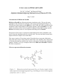
2 How to represent a dislocation structure
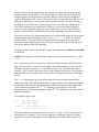
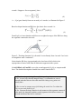
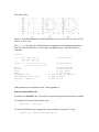
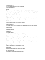
Figure 1 shows a simple approach that can represent an arbitrary dislocation network.
The dislocations are specified by a set of nodes that are connected with each other by
straight segments. Each segment has a nonzero Burgers vector. Because the Burgers
vector is defined only after a sense of direction is chosen for the dislocation line, we can
define bij as the Burgers vector for the segment going from node i to node j. Then bji is
the Burgers vector of the same segment going in the reverse direction, and bij+bji=0.
Under this convention, the conservation of Burgers vectors means that the Burgers
vectors for all the segments going out of every node sum up to zero. These sum rules
provide a useful check for topological self-consistency during the line-DD simulation.
From above we know, the fundamental degrees of freedom in this model are the position
of nodes and the nonzero Burgers vectors: {ri, bij}, i, j = 1, ... , N, where N is the total
number of nodes. The nodes can be positioned anywhere in space, hence the nodal
position ri and the connectivity between the nodes as specified by bij may change from
time to time during a line-DD simulation.
The data structures used to describe these nodes and connections in DDLab and ParaDiS
are different.
In DDLab, the geometry of the dislocation loop is given in two data structures: rn and
links.
The rn data structure gives the position of physical and discretization nodes and their
flags. The size of the rn array is four columns wide and the number of nodes long. The
first three columns contain the x, y, z coordinates of the node, and the fourth column
contains a flag. Currently, there are only two node flag used in the code. A flag equal to 0
means that the node is a regular node, a flag equal to 7 means that the node is immobile
(fixed).
The links data structure gives the information of the discretization segments that
connect the nodes. The “links” data structure is eight columns wide and the total number
of links long. The first two columns gives the nodeids of the starting and ending nodes
of the dislocation segments. The 3rd – 5th columns give the burgers vector of the
dislocation line in Cartesian coordinates, and the 6th – 8th columns give the glide plane of
dislocation segments.
For example, suppose that
rn = [ -500 -500 1000 7;
500 500 -1000 7;
0
0
0
0];
links = [ 1 3 0.5 0.5 0.5 -1 1 0;
3 2 0.5 0.5 0.5 -1 1 0];
This means that there are three nodes in the system, 1, 2, and 3. Node 1 and node 2 are
fixed and node 3 is mobile. There are two segments with Burgers vectors b13 and b32.
From this we see that each segment is only represented once in this data structure. For
example, if b13 is in the links array, then there is no need to include b31 in the links
array as well.
In ParaDiS, the nodal data structure is defined as (in Node.h):
struct _node {
.......
real8 x, y, z;
/* nodal position */
......
int numNbrs;
/* number of neighboring nodes */
real8 *burgX, *burgY, *burgZ; /* Burgers vectors of segments */
real8 *nx, *ny, *nz;
/* Glide plane normal */
......
Tag_t myTag;
/* Tag of node (domainID,index) */
Tag_t *nbrTag;
/* Tag of neighboring nodes */
......
}
Therefore, the data structure in ParaDiS is based on each node. Thus each segment is
represented twice – once in each node connected to this segment.
Detailed description of each data structure can be found in reference [2] and [3].
Q: What are the relative advantages and disadvantages of the DDLab and
ParaDiS data structure?
A: The data structure in DDLab requires less memory because it represents
each segment only once. But if we need to change the connectivity between
nodes, we need to maintain the rn and links array, which is rather
cumbersome to do especially if the number of nodes and segments is large.
In comparison, the nodal data structure in ParaDiS is more flexible and easier
to maintain. This makes ParaDiS more suitable to large-scale simulations.
3 Flow chart of the code
After setting up the initial configuration of dislocation loops and other parameters, both
DDLab and ParaDiS will follow the same algorithm to simulate dislocation dynamics,
as is listed below:
(1) calculate the force of each node
(2) calculate the velocity of each node
(3) calculate the new position of each node
(4) make necessary topological changes
(5) repeat (1) to (4) until the maximum step is reached
The following sections will discuss these steps in more detail.
4 How to calculate the nodal force
There are two ways to calculate the nodal force. The first way is to directly take
derivatives from the total energy. The second way is to use the stress field and the PeachKoelher formula. Both ways should give identical results. In both DDLab and ParaDiS
we use the second approach.
Energy and force
The driving force on each node, say node i, can be defined as the derivative of the total
energy with respect to its position ri, i. e. ,
(1)
In other words, the driving force is the rate of energy drop in response to an infinitesimal,
virtual displacement of node i, while keeping the node connectivity (Burgers vectors) and
other nodal positions constant.
The total energy can be split into an elastic energy term and a core energy term, i. e.
(2)
But since the calculation of core energy requires atomistic input, the core term is usually
ignored in line-DD simulations. We also ignore the core energy term in the following
discussions. Then the relation between force and energy becomes
(3)
From the linear elasticity theory, the elastic energy of a dislocation network can be
expressed in terms of double line integrals along the dislocation
(4)
Since the derivative of R diverges as || x – x' || approaches zero, Eel is infinite. A good
method to solve this problem is to replace every R inside Eq. (4) by
, i.e.,
(5)
where a is the core radius parameter.
For a piece-wise straight dislocationo network as shown in Figure 1, the elastic energy
can be written as a sum of self energies, and interaction energies between the segments,
whose expressions are available in analytic form (Ref. 4).
The nodal forces can be obtained by directly computing the derivatives of these
expressions.
Stress and Peach-Koehler force
The Peach-Koehler formula expresses the elastic force per unit length on the dislocation
line in terms of the local stress field,
(6)
where σ(x) is stress, b and ξ is the Burgers vector and line direction of the segment
respectively.
The self stress field due to a dislocation loop is
(7)
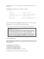
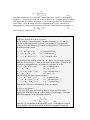
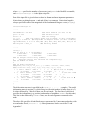
In order to get the relation between PK force and nodal force, we define a shape function
Ni(x) for every node i, and that function is nonzero only if x lies on a segment connected
to node i. Suppose x lies on segment ij, then
(8)
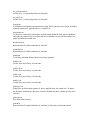
i. e. , Ni(x) goes linearly from zero at node j to 1 at node i, as illustrated in Figure 2.
Based on shape function and PK force, the elastic force on node i is:
(9)
From Eq.(9) we know that the nodal force are weighted averages of the PK force along
the segments connected to the node.
Figure 2: The shape function N2(x) for node 2 varies linearly from 1 at node 2 to 0 at its
two neighbors: node 1 and node 3.
Notice that the PK force is proportional to the local stress field, which is the
superposition of stress fields from all dislocation segments in the system.
In both DDLab and ParaDiS, we use the second approach, Eq.(9), to compute nodal
force. The detailed description of nodal force can be found in Ref. 1.
Q: What does integral along C mean if it is not a loop?
A: If C is not a loop, then the integral along C is evaluated over a set of
directed paths that traverse the entire network visiting every point on it
exactly once.
Q: Do we need to compute stress field along the entire line C to obtain the
force on one node from Eq.(9)?
A: No. Because the shape function is only nonzero at the segments connected
to the node, the integrand vanishes on the segments which do not connect to
the node and do not need to be evaluated.
Q: In both DDLab and ParaDiS codes, nodal force contribution from
interaction between any two segments is computed using a function
[f1,f2,f3,f4]=RemoteNodeForce(x1,x2,x3,x4,b12,b34,a,mu,nu);
in which x1,x2,x3,x4 are endpoints of the two segments, b12 and b34 are the
Burgers vectors of the two segments. a is core radius, mu is shear modulus
and nu is possion's ratio. f1, f2, f3 and f4 are the force on the four nodes.
Can we use this function to compute the self force of a segment 12?
A: Since the singularity is completely removed, the way to calculate self force
is the same as to calculate the force between two different segments, the only
difference is that we need to use the parameters of segment 12 to replace the
parameters of segment 34 in the function call, i.e.,
when using that function, then the function actually becomes
[f1,f2,f1,f2]=RemoteNodeForce(x1,x2,x1,x2,b12,b12,a,mu,nu);
Q: How many times do we need to call the function described above to
compute the force on a given node i, assuming there are totally N segments?
A: Suppose node i is connected to n segments. We need to include the
interaction between these n segments with all N segments to compute the
nodal force on node i. Therefore we need to call the above function nN times.
Q: How many times do we need to call the function described in last problem
to compute the nodal force for all nodes?
A: N2/2 times.
5 Mobility law and nodal velocity
There are several mobility laws to obtain nodal velocity from the nodal force, such as
FCC1, BCC0 and BCC1. To specify FCC1 student in DDLab, the input file should
contain the following line:
mobility = ’mobfcc1’;
To do so in ParaDiS, then the input file should contain:
MobilityLaw = ”FCC_1”
The detailed description of mobility law can be found in Ref. 1.
In the following, we discuss the FCC1 mobility law in more detail as an example.
In FCC1, the nodal velocity and nodal force are related by,
(10)
where the summation is over all nodes j connected to node i, and Lij is the length of
segment i-j. B is the drag coefficient, which is taken to be a constant (unity) in DDLab.
This means that the mobility anisotropy (e.g. between edge and screw dislocations) is
ignored here. After the nodal velocity is computed from Eq.(10), it needs to be
orthogonalized with respect to all normal vectors nij of the neighboring segments, i.e.,
(11)
for every node j connected to i.
Q: If node i is connected to several segments, how to orthogonalize vi with all
glide plane normals nij of these segments?
A: For example, assume that node 1 has three segments, 1-2, 1-3 and 1-4,
with three glide plane normal vectors n12, n13 and n14. A naïve approach
would be to use the following procedure to orthogonalize v1 with respect to
these three normal vectors.
v1’ = ( I – n12 ⊗ n12 ) * v1
v1’’ = ( I – n13 ⊗ n13 ) * v1’
v1’’’= ( I – n14 ⊗ n14 ) * v1’’
( v1’ is normal to n12)
( v1’’ is normal to n13)
( v1’’’ is normal to n14)
The problem of this method is that if n12, n13 and n14 are not normal to each
other, the final velocity v1’’’ may be not normal to n12 and n13. Therefore we
first need to orthogonalize n12, n13 and n14 to each other. If we let,
n13’ = ( I – n12 ⊗ n12 ) * n13
( n13’ is normal to n12)
n13’’ = n13’ / || n13’||
( if || n13’|| > 0)
n14’ = ( I – n13’ ⊗ n13’ ) * n14
( n14’ is normal to n13’)
n14’’ = n14’ / || n14’||
( if || n14’|| > 0)
and then follow the same sequence as above:
v1’ = ( I – n12’’ ⊗ n12’’ ) * v1
( v1’ is normal to n12)
v1’’ = ( I – n13’’ ⊗ n13’’ ) * v1’
( v1’’ is normal to n13’’)
v1’’’= ( I – n14’’ ⊗ n14’’ ) * v1’’
( v1’’’ is normal to n14’’)
Then the final velocity is orthogonal to all n12, n13 and n14.
Q: How to calculate nij?
A: Since the glide plane includes both Burgers vector and dislocation
segment, the normal direction nij will be normal to both Burgers vector and
dislocation segment, so the glide plane normal is,
(12)
From Eq. (12) we find that if the segment is screw, i.e. the Burgers vector is
nearly parallel to the line direction, nij in the above equation becomes ill-
defined. Physically, this corresponds to the fact that the motion of screw
dislocation is not confined to a plane. Correspondingly, in this case, we may
not need to orthogonalize nodal velocity with any plane normal vector (this is
the case for the BCC0 mobility law, the FCC0 case is different as discussed
below).
Q: What is the difference in nij between FCC and BCC mobility laws?
A: From above we have seen that for a screw dislocation, a glide plane cannot
be uniquely defined. Thus in BCC crystals, the screw dislocation is equally
likely to move on several planes. However, in FCC crystals, even screw
dislocations may have a preferred glide plane because of the existence of lowenergy stacking fault on certain planes. Consequently, the dislocation core
prefers to spread itself on one of those planes (in the form of two partial
dislocations bounding a stacking fault area), so the dislocation motion is
confined to the chosen plane. To account for this core property in the code,
each segment i-j may carry an extra variable nij that represents the normal
vector of the chosen glide plane. nij may be given as part of the initial
condition. During the simulation, the glide planes can remain unchanged, or it
can be changed stochastically to model the cross slip event.
6 Topological changes
For numerical and physical reasons, line-DD simulations need to handle topological
changes, i.e. changes on the connectivity between nodes since we may want to adjust the
number of nodes that represent a dislocation line if the line gets longer or shorter during
the simulation, or when two dislocation lines meet in space, they may either annihilate or
zip together to form a junction, which also results in a change of nodal topology.
Thus many types of topological changes can be encountered in a line-DD simulation.
Fortunately, since we use a nodal representation here, all topological changes can be
implemented through two basic operators: merge (two nodes merge into one ) and split
(one node split into two ). The implementation of these two operators is straightforward
– all one needs to do is to make sure that at the end of the operation the Burgers vector
sum rule at every node and segment is still satisfied, moreover, two nodes are either
disconnected or connected only once, and each node is connected with at least two other
nodes, if a node has no segment, it will be deleted.
Detailed description of merge and split operation can be found in Ref. 1.
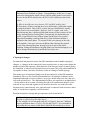
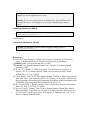
Q: If a node has many ways to split, how do we determine which way to split
the node or shall we keep the node intact?
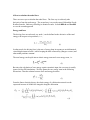
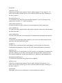
A: For example, for a 4-arm node such as P’ in Figure 3, there are 3 different
ways to partition its arms: (12)(34), (13)(24) and (14)(23). It is reasonable to
expect that the way nature would choose should be the one that gives rise to
the maximum energy dissipation rate, which is defined below.
Figure 3: A node P’ with 4 arms, 1, 2, 3 and 4.
Suppose an n-arm mode i stays intact (not splitting) and it feels a force fi and
will move at velocity vi. Then the local energy dissipation rate is,
(13)
Now suppose that node i splits into two nodes P and Q, such that node P
retains 1,…,s of the original neighbors, and node Q retains the remaining
neighbors. Let fP and fQ be the forces on the two nodes and vP and vQ be their
velocities given by the mobility function. Then the local energy dissipation
rate is,
(14)
If
, then node i prefers to split into two nodes P and Q instead of
moving as a single node. The energy dissipation rate can be computed for all
possible (topological distince) modes to split i. The mode with the highest
energy dissipation rate is preferred.
b. When we split one node into two nodes, where are the two new notes
physically located?
If a node will split in next step, the two new nodes actually stay at the same
location as the “parent” node at the current step. Because the velocities of the
two nodes is different (otherwise the node should not split), the two nodes
will be move away from each other in the next time step.
7 How to run DDLab
In order to execute the code, we need to first set the necessary parameters, dislocation
configuration, then run dd3d.m to start the dislocation dynamics simulation.
For example, if we want to simulate a Frank-Read source and frinit.m contains the
initial condition data, then in the MATLAB command window, we type:
>> frinit
>> dd3d
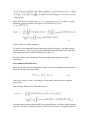
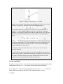
The result will be
Figure 4: Line-DD simulation of Frank-Read source at (a) cycle N=20, (b) cycle N=100,
and (c) cycle N =150.
File frinit.m specifies the initial dislocation configuration and simulation parameters.
Part of the file is listed below. Notice that everything between % and end of line is a
comment.
frinit.m
rn = [ -500 -500 1000 7;
%% see section 2
500 500 -1000 7;
0
0
0
0];
links = [ 1 3 0.5 0.5 0.5 -1 1 0;
%% see section 2
3 2 0.5 0.5 0.5 -1 1 0];
MU=1.0;
%% shear modulus
NU=0.3;
%% poisson’s ratio
a=0.1;
%% core radius
Ec=0;
%% core energy
totalsteps =300;
%% total steps of simulation
appliedstress = zero (3,3);
%% applied stress
mobility = ’mobfcc1’;
%% mobility law
......
Other parameters are explained in Ref. 2 and Appendix A.
8 How to run ParaDiS code
In order to run ParaDiS code, we need first compile the program then run the executable.
To compile on a Linux (i686) machine, type,
make dd3d
SYS= Linux
To run a Frank-Read source example (the same problem as in Section 7), type,
mpirun –np 1 dd3d Tests/fccFRsingle.cn
where -np 1 specifies the number of processors (one), dd3d is the ParaDiS executable,
and Tests/fccFRsingle.cn is the input script file.
Part of the input file is given below to show its format and most important parameters.
Notice that everything between # and end of line is a comment. Notice that length is
always specified in unit of the magnitude of the fundamental Burgers vector (burgMag).
Tests/fccFRsingle.cn
......
ShearModulus = 54.6e9
### shear modulus (in unit of Pa)
pois = 0.324
### Poisson’s ratio
Ecore = 0
### core energy
rc = 0.1
### core radius (same as a in DDLab, in unit of burgMag)
burgMag = 2.725e-10 ### magnitude of Burgers vector (in unit of meter)
appliedStress=[ 0 0 0 0 0 4e8] ### [σ11, σ22, σ33, σ23, σ13, σ12] in Pa
mobilityLaw = ”FCC_1”
### mobility module
......
config = [
### (1) Box X, Y, Z (in burgMag )
-17500.0000
-17500.0000
-17500.0000
17500.0000
17500.0000
17500.0000
### (2) Burgers vector array (number)
0
(obsolete option, but retained for compatibility)
### (3) Number of nodes
3
### (4) Nodal information
###(primary line: node_id, old_id, x, y, z, numNbrs, constraint, domain, index)
###( second line: nbr[i], bx[i], by[i], bz[i] nx[i], ny [i], nz[i])
1 0 500.0 6000.0 4000.0
1
7
0
0 ### in unit of burgMag
2 -0.5773503
-0.5773503
0.5773503
-1
1
0
2 0
500.0 6000.0 0.0
2
0
0
1
%% the unit is b
1
0.5773503
0.5773503
-0.5773503
-1
1
0
3
-0.5773503
-0.5773503
0.5773503
-1
1
0
3
0
500.0 6000.0 -4000.0
1
7
0
2
%% the unit is b
2
0.5773503
0.5773503
-0.5773503
-1
1
0
......
]
The dislocation structure is specified in the config = [ ...... ] complex. The nodal
information starts in section (3), which first gives the total number of nodes (here it is 3).
It is then followed by 3 blocks of data, one for each node. The first line of each block
specifies the information (e.g. position, and number of neighbors numNbrs for this node).
This line is then followed by numNbrs lines, one for each segments connected to the
node.
The above file specifies a Frank Read source represented by 3 interconnected nodes, with
two end nodes fixed (constrain = 7). Other parameters can be seen in Ref. 3 and
Appendix C.
Exercise: After the FR source have emitted a dislocation loop, what will
happen if we set the applied stress to zero?
Exercise: Try to reverse the direction of applied stress, what will happen for
the same FR source? Is the Burgers vector of the emitted loop the same as
before?
9 Junction simulation in DDLab
Exercise: Use DDLab to run the junction zipping example given in
inputgeombinaryjunction.m
fccjunc-init.cn
10 Junction simulation in ParaDiS
Exercise: Use ParaDiS to run the junction zipping example given in
Tests/fccjunc-init.cn
References:
[1] Line-Dislocation Dynamics, Chapter 10 in Computer Simulation of Dislocations,
Vasily V. Bulatov and Wei Cai, Oxford University Press, in preparation.
[2] DDLab Primer, Tom Arsenlis and Wei Cai, 2005.
[3] ParaDiS User's Manual, Masato Hiratani et al., Lawrence Livermore National
Laboratory, 2005.
[4] W. Cai, V. V. Bulatov, J. Chang, J. Li, and S. Yip, Dislocation Core Effects on
Mobility, in F. R. N. Nabarro and J. P. Hirth, ed. Dislocations in Solids, NorthHolland Pub. vol. 12, p. 1 (2004).
[5] Vasily Bulatov, Wei Cai, Jeff Fier, Masato Hiratani, Tim Pierce, Meijie Tang, Moono
Rhee, Kim Yates, Tom Arsenlis, Scalable Line Dynamics in ParaDiS, Conference on
High Performance Networking and Computing, Proceedings of the Proceedings of the
ACM/IEEE Super Computing 2004 Conference (SC'04), p. 19.
[6] Wei Cai and Vasily V. Bulatov, Mobility Laws in Dislocation Dynamics Simulations,
Mater. Sci. Eng. A, 387-389, 277 (2004).
[7] Wei Cai, Vasily V. Bulatov, Tim G. Pierce, Masato Hiratani, Moono Rhee, Maria
Bartelt and Meijie Tang, Massively-Parallel Dislocation Dynamics Simulations, in
Solid Mechanics and Its Applications, H. Kitagawa, Y. Shibutani, eds., vol. 115, p. 1,
Kluwer Academic Publisher 2004.
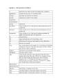
Appendix A Main parameters in DDLab
Appendix B Main subroutines in DDLab
addline.m
Add a straight line onto nodal structure rn, links
addloop.m
Add a dislocation loop onto nodal structure rn, links
addrandloop.m
Add a random dislocation loop
bob.m
A dislocation configuration and parameter setting file for core structure, including
materials parameters, applied stresses, viewpoint, etc.
cleanupnodes.m
Cleanup the empty node and link entries
collision.m
Merge nodes if certain conditions are satisfied
consistencycheck.m
To check whether the burgers vector is consistent
constructsegmentlist.m
dd3d.m
The main code to simulate the dislocation dynamics which includes calculating the forces
on the dislocation line segments, updating the positions of nodes, performing topological
changes and remeshing the system as needed.
drndt.m
Get the force and velocity of each node
fccjunc_step500.mat
A dislocation configuration and setting file for junction of two line segments, including
applied stresses, viewpoint, etc. ( no parameter setting)
FieldPointStress.m
Calculate the stress at one point due to one segment
findcollisionpoint.m
To find the collision point of two nodes given that there are strict glide plane contraints
findfsegcomb.m
findsgeforcemajor.m
findsubfseg.m
To find the subforce
of each segment, used in choosing the way of splitting
frinit.m
A dislocation configuration and parameter setting file for FR source, including materials
parameters, applied stresses, viewpoint, etc.
frsource.mat
A dislocation configuration and setting file for FR source, including applied stresses,
viewpoint, etc. ( no parameter setting)
genconnectivity.m
Generate the connectivity list from the list of links
initparams.m
Default parameter settings ( no configuration setting)
int_eulerbackward.m
Get the force, velocity and position of each node
int_eulerforward.m
Get the force, velocity and position of each node
int_ode15s.m
Get the force, velocity and position of each node
juncinit.m
A dislocation configuration and parameter setting file for junction of two loops, including
materials parameters, applied stresses, viewpoint, etc.
mergenodes.m
To merge the connectivity information in nodeid with deadnode, then remove deadnode
and repair the connectivity list and the link list so that there are no self links and no two
nodes are linked more than once
meshcoarsen.m
Remesh nodes if certain conditions are satisfied
meshrefine.m
Remesh nodes if certain conditions are satisfied
mindist.m
To find the minimum distance between two line segments
mobbcc1.m
Get the force and velocity of each node
mobbcc1b.m
Get the force and velocity of each node
mobfcc0.m
Get the force and velocity of each node
mobfcc1.m
Get the force and velocity of each node
pkforcevec.m
Nodal force on dislocation segment 01 due to applied stress, the output is a 1*6 matrix,
the first three columns give the force on node 0 and the last three columns give the force
on node 1
plotnodes.m
Plot dislocation structure
remesh.m
Remesh nodes if certain conditions are satisfied, it is the sum of meshcoarsen and
meshrefine
remoteforcevec.m
Nodal force on dislocation segment 01 due to another segment 23, the output is a 1*6
matrix, the first three columns give the force on node 0 and the last three columns give
the force on node 1
RemoteNodeForce.m
To calculate the force between two dislocation segments 12 and 34, the output is the
remote force on nodes 1, 2, 3 and 4 respectively
removedeadconnection.m
To delete an entry in a node's connectivity list and update the linksinconnet array
removedeadlink.m
To replace the link in linkid with the link in llinks, repair the connectivity and then delete
the llinks from links
removedeadnode.m
To remove the nodes that are no longer part of simulation and cleanup the data structure
removelink.m
To delete the link information from connectivity list, remove the link from the link list
and replace the linkid with the last link
rundd3d.m
A whole code to simulate the dislocation dynamics, which includes the dislocation
configuration and parameter setting, the run mode control and dynamics simulations
segforcevec.m
Nodal driving force of each segment. It is a n*6 matrix, n is the number of segments, the
first three columns give the force on the first node and the last three columns give the
force on the second node. It is the sum of pkforcevec, selfforcevec and remoteforcevec
SegSegInteractionEnergy.m
To calculate the interaction energy between two segments
selfforcevec.m
Nodal force on dislocation segment 01 due to itself (self stress), the output is a 1*6
matrix, the first three columns give the force on node 0 and the last three columns give
the force on node 1
separation.m
Split nodes with 4 or more connections if certain conditions are satisfied
splitnode.m
Split the connectivity of nodeid with a new node that is added to the end of rn after the
node is added.
writeParaDiS.m
Write rn, links into ParaDiS restart file format
zip.m
A dislocation configuration and parameter setting file for core structure, including
materials parameters, applied stresses, viewpoint, etc.
zip2.m
A dislocation configuration and parameter setting file for core structure, including
materials parameters, applied stresses, viewpoint, etc.
ziponefcc1.m
A dislocation configuration and parameter setting file for a specific structure, including
materials parameters, applied stresses, viewpoint, etc.
ziptotom.m
A dislocation configuration and parameter setting file for core structure, including
materials parameters, applied stresses, viewpoint, etc.
Appendix 3 Main parameters in ParaDiS
(to be completed)
Appendix4 Main subroutines in ParaDiS
(to be completed)