Download Printer-friendly Version

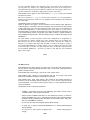
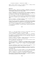
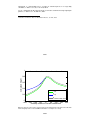
Instrumentation
Methods and
Data Systems
Open Access
Open Access
Instrumentation
Methods and
Data Systems
Discussions
Geoscientific
Model Development
Discussions
Open Access
Open Access
Hydrology and
Earth System
Sciences
Open Access
Hydrology and
Earth System
Sciences
Open Access
Geosci. Model Dev. Discuss., 6, C667–C698, 2013
Geoscientific
www.geosci-model-dev-discuss.net/6/C667/2013/
© Author(s) 2013. This work
is distributed
under
Model
Development
the Creative Commons Attribute 3.0 License.
Discussions
Discussions
Discussions
Open Access
The Cryosphere
Open Access
The Cryosphere
Received and published: 29 May 2013
Open Access
[email protected]
Open Access
A. K. Miltenberger et al.
Discussions
Open Access
Open Access
Interactive comment on “An online trajectory
Ocean Science
Ocean
Science
module (version
1.0)
for the non-hydrostatic
numerical weather prediction model COSMO” by
A. K. Miltenberger
et al.
Solid Earth
Solid Earth
We thank both referees, Ulrich Blahak and Petra Seibert, for their extensive and
very constructive reviews. Both reviews were very useful for improving the module
description as well as the discussion section of the paper. As some aspects are
discussed several times at different places in the two reviews, we choose to bundle
our reply to these comments.
C667
1. Neglect of diffusive processes / Lagrangian parcel vs. Lagrangian particle
models
Both referees allude to the aspect that our model does not consider subgrid scale
(turbulent) processes for the calculation of the trajectories:
Ulrich Blahak C197/C198: The authors strongly advocate the Lagrangian perspective
also for very high resolution applications. However, diffusive processes are completely
neglected in the new module. Therefore it is questionable and will depend on the
application, if there is really a big gain in “physical” accuracy, if nontheless trajectories
are interpreted as coherent air parcels over several days. Therefore, what I miss
is a more thorough discussion of the influence of diffusive processes. Results of
this module might be misleading for, e.g., applications in high resolution dispersion
modeling. What is the advantage of doing online trajectories when one could use
artificial tracers in the model to simulate advection and diffusion simultaneously?
Ulrich Blahak C198: While this may justify publication in GMD, the comparatively
simple numerical implementation (e.g., no turbulent fluctuations on the trajectories)
could have some implications for some applications like dispersion modeling or
analysis of strongly turbulent flows in convective clouds. This fact should be elaborated
more in the paper.
Ulrich Blahak C199: Consequences of the neglect of diffusive processes - As mentioned above, please add in section 1 and/or in section 4 (at places where you think
it is appropriate) short discussions on the influence of turbulent diffusive processes
and the consequences, if these are neglected and if the trajectories are interpreted
as coherent air parcels over long times. Discuss which kind of applications, at which
spatial/temporal scales, potentially could suffer from this neglect and to what extent.
One example of a paper applying an autoregressive Markov process to represent
turbulent fluctuations on trajectories for high-resolution Monte Carlo dispersion modeling would be Gross, H. Vogel, F. Wippermann, 1987: Dispersion over and around a
C668
steep obstacle for varying thermal stratification – numerical simulations, Atmospheric
Environment, Volume 21, Pages 483-490.
Petra Seibert C 358: Another reviewer has questioned the value of mean-wind
trajectories at the spatial scale covered by the model. Also the authors allude to this
issue in their discussion of the behaviour near ground. My opinion is that a trajectory
model (this is the term that I am using for a mean-wind-based model, as opposed to
a Lagrangian particle model which would simulate also the effects of subgrid-scale
motions) does have its place also at high resolution (even at LES scale) as it allows
to investigate atmospheric motion patterns represented explicitly in the model in a
way that cannot be achieved e.g. by a Eulerian tracer carried (unless a number of
tracer species is used which is the same as the number of trajectories, but even then
diffusive properties of the numerical integration would deteriorate the result). However,
I think the authors could invest some additional work to include a survey of possible
application types, the set-ups related to them, and their merits and shortcomings. This
would be a significant benefit for users beyond their own group and enhance the value
of the paper.
It is true that our trajectory model does not consider diffusive processes, but this is
also not the goal of our study. For applications like dispersion modeling there are other
(better) tools and methods like Lagrangian particle dispersion models and passive
tracer models, which aim to represent subgrid-scale processes. In the following we
refer to trajectory models neglecting diffusive processes as Lagrangian parcel models,
while those representing subgrid-scale velocity variations are named Lagrangian
particle (dispersion) models (LPDMs).
The two approaches - Lagrangian parcel and particle dispersion models - have
different strengths and weaknesses and are therefore suitable to investigate different
scientific questions. Therefore we agree with the second referee, Petra Seibert, that
the Lagrangian parcel model approach has its validity also for high-resolution modeling
and even LES.
C669
The Lagrangian parcel model represents the average properties of an air parcel with
a typical volume of a grid cell. The motion of such an air parcel represent the mean
of a particle plume starting within a grid box in a Lagrangian particle model. As noted
for instance by Stevens et al. (1996) and utilized in trajectory-based moisture source
diagnostics (Sodemann et al. 2008), the time average result of mixing is represented
on the scale of gridboxes along parcel trajectories. Therefore on temporal scales that
are in agreement with the gridspacing and the advection velocity, the variation in a
finite size box is well captured by the parcel model. If subgrid scale variations and
according timescales are the focus of the study, then of course Lagrangian particle
dispersion models are the tool of choice. Note that then a much larger number of
particles must be calculated (compared to the number of parcels with our approach)
in order to statistically sample the subgrid-scale variations. For instance, as illustrated
in the Stevens et al. (1996) study on timescales in non-precipitating stratocumulus
clouds, a microphysical boxmodel driven with a Lagrangian parcel model may have
problems at cloud edges as warming and drying rates of individual parcels may be
too strong due to the neglect of subgrid-scale variations in humidity and temperature.
Nevertheless parcel models are successfully used in the literature for Lagrangian
analyses of LES simulations (e.g., Yeo and Romps, 2013). In contrast to LPDM they
allow to study the influence of non-resolved mixing be it from parameterizations or
numerical diffusion on the mean properties of air parcels. In addition, as Yeo and
Romps (2013) pointed out, air parcel trajectories ensure a constant mass of dry air
associated with the trajectory, while this is not the case if subgrid-scale velocities are
additionally taken into account.
In addition it is important to keep in mind that the represented processes using
mean-wind trajectories strongly depend on the grid-spacing and hence is different
from LES to NWP applications: While it may be inappropriate (or impossible) to study
deep convection with a Lagrangian parcel model in a NWP model that does not resolve
convective processes, it is justified in convection resolving models.
Lagrangian particle models have been specifically developed to investigate the
C670
dispersion of pollutants in the turbulent boundary layer, where subgrid-scale velocity
variations are particularly important. Outside of the planetary boundary layer turbulence becomes less important and therefore the solution of Lagrangian particle models
and Lagrangian parcel models should converge.
Online trajectories aim to represent the motion of air parcels as accurately as possible,
according to the resolved scale wind field. Thereby the air parcels are not regarded as
“closed boxes”, but as permeable for subgrid-scale motions, which they do not aim to
represent explicitely. If the latter is the objective of a study, then Lagrangian particle
models must be used. The differentiation between sub-grid scale processes and the
resolved wind is fundamental, although it relates to different scales and processes for
different model resolutions.
We acknowledge that it is important to discuss the difference between the two
approaches in the paper together with their advantages and disadvantages for certain
scientific questions. As suggested we will add a note in the introduction and an
additional paragraph on this issue in the discussion section.
2. Representativity of literature in the introduction section
Ulrich Blahak C196/197: All in all, the authors reference an adequate quantity of literature concerning applications in synoptic meteorology, which is their field of expertise.
There are less citations of the more technical aspects of trajectory calculations, as well
as of applications in other fields like lagrangian dispersion modeling. For the scope of
this paper, this should however be fine.
Petra Seibert C359: The list of possible applications of Lagrangian, trajectory-based
analyses is obviously only meant to give some illustrations, but in the light of my remarks above on applicability of this specific high-resolution trajectory model, they may
want to give more consideration specifically to high-resolution applications.
We will include a few more references on high-resolution applications. Specifically we
C671
want to include the following studies in the introduction as examples how trajectories
have been successfully used in high-resolution models:
a) Lagrangian parcel model applications in high-resolution NWP models
• Stern et al. (2013) investigated the motion of parcels inside the eye of an idealized hurricane by calculating trajectories based on one to six minute NWP output.
• Wang and Xue (2012): trajectories based on one-minute NWP output were employed to determine the origin of air parcels feeding initial convective cells. The
study investigates convective initiation cases associated with a cold front dryline
system from the IHOP field project.
• Fierro et al. (2009): In idealized simulations of a nocturnal equatorial oceanic
squall line (online) trajectories are used to investigate the hot tower hypothesis.
The study concludes based on the evolution of equivalent potential temperature
and latent heating along the trajectories that most parcels experience mixing at
low-levels and that the associated loss of buoyancy is compensated by latent
heat release from ice processes.
b) Lagrangian parcel model applications with LES
• Yamaguchi and Randall (2012): This study of cloud-top entrainment in marine stratocumulus boundary layer clouds employs a Lagrangian parcel-tracking
model online in a LES. Though for this model a parameterization of sub-gridscale
velocities is available it is not used in the study, as the authors found it to have
negligible effect on the trajectories.
• Stevens et al. (1996): In this study of non-precipitating stratocumulus clouds
trajectory ensembles calculated with LES resolved winds were used as driving
C672
conditions for a microphysical parcel model. Besides the illustration of the usefulness of the approach to investigate critical timescales for droplet growth, the
paper provides a discussion of the representation of entrainment and its effect on
microphysical modeling.
• Kogan (2006): This study used the approach of Stevens et al. (1996) for drizzling
stratocumulus clouds. The in-cloud residence time is found to be 2-5 times longer
than for non-drizzling stratocumulus indicating that cycling of air parcels inside the
cloud is important for drizzle formation.
• Yeo and Romps (2013) computed trajectories with the resolved wind to study
entrainment rates and residence times in convective clouds.
c) Lagrangian Particle Dispersion models
• Bellasio et al. (2012) described a long-range Lagrangian particle dispersion
model developed for simulating radioactive clouds. The paper comprises a comparison to the ETEX tracer release experiment.
• Weil et al. (2012) coupled an LPDM to a LES for investigation of plume dispersion
in a convective planetary boundary layer.
• Gross et al. (1987): Description of the simulation of pollutant dispersion from a
point source around a steep obstacle.
Petra Seibert C361: Page 1229: I am wondering whether there are no more recent
applications of LAGRANTO than 2005.
Of course there are numerous more recent applications of LAGRANTO, but the list
was meant to indicate the spectrum of applications for which it has been used. But of
course we can in addition name a few more recent papers, as for instance Lefohn et
C673
al. (2011), Cirisan et al. (2013), Schemm et al. (2013), and Grams et al. (2013).
3. Terrain intersecting trajectories
Ulrich Blahak C198: The authors honestly highlight one remaining technical problem
of their new online trajectory module, namely that too many trajectories intersect the
ground, especially in mountaneous regions. Currently this problem is mitigated by
the standard method of simply reinitializing ground-hitting trajectories 10 m above the
ground. However, the deeper reasons for this behaviour are not very well explained,
and this should be improved in the manuscript. This is important for future users of the
module to decide whether this fact is acceptable for their application or not. Without
beeing a detailed expert, I would presume that there can be found something in the
literature on this topic.
Ulrich Blahak C 203/204: Issue with too many trajectories hitting the ground, starting at
p. 1242, line 9: Although I can follow your argument with linear interpolation smoothing
the wind- field (presumably especially the vertical compontent) and beeing responsible
for curving down your example trajectories in figure 6 towards the surface, the exact
behaviour near the surface should depend on details of what is assumed for the windfield close to the surface and how this interplays with a possible violation of the vertical
CFL criterion (see above, in this case with ∆z = vert. distance to the ground).
However, I do not understand figure 6 because of missing information. What are the
axis labels, what is the grid spacing of the Eulerian framework? 1000 X-units as suggested by the crosses on the orography line? What is the online timestep resp. the
“typical” online travel distance during 1 timestep? What exactly is the windfield (you
only mention in the figure caption, that it is linear. But at which value does it start at the
surface? All this information is necessary to understand why the online trajectory can
hit the ground. And I do not understand why it can continue below the surface. Should
it not end on impact, i.e., when its position first falls below the orography during the
C674
Petterssen scheme iteration?
From this I conclude that the surface-normal wind compontent does not go to 0 towards
the ground and that there is an artificial non-zero velocity below the surface, so that the
iteration may continue there and eventually may converge to a final position above the
surface. Is that true? If yes, how is this calculated? Constant extrapolation from the
lowest model level?
Petra Seibert C361: The ground intersection problem should not be introduced as the
second-last paragraph of the whole paper! It belongs into the module description.
We agree that it is probably not best to discuss the ground intersection problem in
the discussion section. In the revised version we will include a section in the module
description with an extended discussion of the problem. As promised below we will
also include a description of the lower boundary condition and we will improve the description of our idealized example. However, we do not think that the lower boundary
condition itself is causing the terrain intersection problem.
In the meanwhile we did some further analysis to pin down the problem of ground intersecting trajectories: For all trajectories that hit the surface in the COSMO7 simulation
of our case-study, the surface elevation as well as the height of the lowest model level
are traced along the trajectories in the last 200 time-steps before ground intersection.
In addition the surface elevation, that would be beneath the trajectory if it continued
in the same direction and speed as during the last timesteps before the terrain intersection was computed for the next 200 time-steps. From this data a composite of the
surface elevation, the lowest model level height and the trajectory height was derived
by normalizing and averaging the data. This composite shows the average surface
elevation 200 time-steps before the ground intersection and its extrapolated behavior
for the 200 time-steps after the ground intersection (Fig. 1). The distance, that the
trajectories travel during these about 400 time-steps corresponds to approximately 3
to 6 grid points.
As this composite closely resembles our hypothetical example in the original paper,
C675
it supports our original hypothesis that the majority of ground intersections occur due
to errors introduced by spatial horizontal interpolation. Reducing the time-step of the
trajectory integration so strongly, likely leads to a more frequent detection of terrain
intersections and therefore leads to an increased percentage of terrain hitting trajectories.
The hypothesis linking the ground intersection to the spatial interpolation, is also supported by our analysis of the vertical Courant number (Fig. 3). The vertical CFLcriterium is never exceeded in the COSMO2.2 and COSMO14 simulations and in the
COSMO7 simulation only very rare exceedances are registered.
Ulrich Blahak C204: On p. 1243, starting in line 5, some possibilities for mitigating
this problem are shortly mentioned. Perhaps you could elaborate a little more on the
possible changes to the integration scheme close to the surface, in addition to adding
turbulent fluctuations. Could these be
• Alternative starting value for the Petterssen iteration (see above)?
• Sub-timestepping near the ground so as to keep the vertical CFL < 1 (see above),
using suitable time interpolation of u?
• Changes to the lower boundary condition(s)?
We will include some discussion of such a modification of the integration scheme close
to the surface.
Petra Seibert C361: I am surprised that consideration of turbulence is offered as
possible way to overcome the ground intersection problem. I don’t see why this should
be effective. On the other hand, this would totally change the character of the model,
and transform it from a trajectory model to a dispersion model. This would be a big
step, in concept but also in terms of algorithm and code. Introducing turbulent diffusion
in only a part of the boundary layer (if this is meant) would be quite unphysical.
C676
After the further investigations we did, we agree that adding turbulence is not the
solution to the problem. We will remove this point from our suggestion list.
4. Structure of module description
Petra Seibert C358: However, the description of the module should be made more
detailed and better structured. It would also be useful to better explain (and maybe
explore) certain decisions and their consequences.
Petra Seibert C359: Module description. I have the following suggestions for improving:
• First, summarise the algorithms used in LAGRANTO, and clearly point out where
additional details (if not included) can be found (is the Wernli and Davies paper
fully comprehensive? If not, add other source, or add corresponding document
as supplementary material).
• Then, give an overview where the COSMO module deviates from the off-line
version.
• Finally, give the details on the COSMO-specific features.
Unfortunately, though not fully comprehensive, the Wernli and Davies paper is the
only and latest technical reference for LAGRANTO. However, we describe all essential
algorithms used in the section “Physical Core“. There the numerical procedure to
integrate the trajectory equation and the interpolation method are described. This
section corresponds to the first section suggested by Petra Seibert.
The COSMO module only deviates from the LAGRANTO algorithms in not using
a temporal interpolation and in being parallelized (see section “Parallelization and
Communication“). Both of these issues are discussed in the paper. There are little
COSMO-specific features. The code developed for this project should be applicable
C677
to any NWP model that has a spatial domain decomposition for the parallelization.
Only the technical details of writing the output file (addressing of variables) as well as
probably the input structure have to be slightly adapted. We will make this clearer in
the revised paper.
Petra Seibert C360: Section 2.3: I would call this “selection of trajectory starting
points” instead of “initialisation”. The fact that back trajectories are not (easily) possible
for on-line calculation needs to explained already in the introduction, and then be
discussed in the Section on applications that I propose. I disagree with the statement
that this limitation “slightly complicates” studies (page 1241 bottom) – it is a limitation!
We will include this fact in the introduction. Of course it is a limitation that only forward
trajectories can be calculated, but we think it is not really tremendously difficult to find
a suitable starting region, if one is interested in trajectories ending at a certain location.
5. Issues related to details of the implementation
Ulrich Blahak C199/200: Presentation of the Petterssen Scheme and its implementation in section 2.1 You present the Petterssen scheme in a way which is customary
in the literature as a kind of predictor-corrector-method. I think your term “iterative
forward Euler timestep” from page 1230, line 5, is wrong. However, in my view it would
be more enlightening to present it slightly differently:
To solve the trajectory equation ~x˙ = ~u(~x(t), t) numerically forward in time from time ti
to ti+1 , a second order semi-implicit discretization in space and time is used, which
reads
˙
˙
~x(ti+1 ) = ~x(ti ) + ∆t ~x(~x(ti ),ti )+~x2(~x(ti+1 ),ti+1 ) = ~x(ti ) + ∆t ~u(~x(ti ),ti )+~u2(~x(ti+1 ),ti+1 )
This is an implicit equation for ~x(ti+1 ), because the last differential on the right-hand
side ~u(~x(ti+1 ), ti+1 ) depends itself on x(ti+1 ). A common method to solve such a
problem numerically is a fixpoint iteration. The above equation is alread in fixpoint
form, so all we need is a starting value ~x0 (ti+1 ) resp. ~u(~x0 (ti+1 ), ti+1 ). Then the n-th
C678
iteration step is given by ~xn (ti+1 ) = ~x(ti ) + ∆t~u(~x(ti ), ti ) + ~u(~xn -1(ti+1 ), ti+1 ) 2 which
equals your second through n-th equation on page 1230. The convergence properties
of such an iteration depend on the properties of the flow field and the starting value.
In your case, the starting value has been simply chosen as ~u(~x(ti ), ti ), so that your
Eq. (1) is recovered. However, you would be basically free to choose different starting
values. For example, near the ground, ~u(~x0 (ti+1 ), ti+1 ) = 0 could help to reduce the
problem of terrain hitting trajectories during the first iteration step.
We will change the naming of the numerical procedure. We thank the reviewer for
offering an alternative description of the scheme, but since we regard our original
presentation more intuitive, we decided not to change it. The result of both derivations
is equivalent.
Ulrich Blahak C200/201: Detailed specification of the lower boundary condition(s)
I miss a detailed specification of the lower boundary condition(s) for computing the
linear spatial interpolations of the velocity components near the ground. These
are decisive for the behaviour of trajectories near the ground and should be clearly
mentioned, so that future users may decide on the applicability of the module for their
specific application. Add a paragraph in section 2.1 or an own subsection, whichever
you feel
Details of these lower boundary conditions could also be responsible for the problem
of too many trajectories hitting the ground (see below). Which boundary conditions
are assumed in other trajectory schemes from the literature?
We extrapolate the horizontal wind velocity below the lowest model level with the same
algorithm used to determine the lower boundary condition for the vertical velocity in
the dynamical core of COSMO. Namely the velocity at some height z below the lowest
model level is calculated by linear extrapolation of the difference between the two
lowest model levels. We will add this information in section 2.1.
Ulrich Blahak C199: Please specify somewhere here, that the COSMO-model uses a
C679
staggered Arakawa C-grid and is formulated in terrain following and rotated spherical
coordinates, because this is important for the spatial interpolation procedure and the
portability of the module to other NWP or climate models.
We will add a sentence in the description of the COSMO model including these details.
In addition we add a paragraph on the portability of the module in section 2.
Ulrich Blahak C199: At the end of this secion, you mention “the trace variables”,
but this important part of the module is not explained further. Please add a short
paragraph on this aspect and on its applications, starting perhaps on p. 1229, line 8.
Paragraph will be added.
Ulrich Blahak C204: Discussion on the properties of the new module and possible
enhancements in the future - You mention that you apply tri-linear interpolation in
space (p. 1230, line 23), and this is perfectly fine. I presume this means that the
interpolation is done between the 8 neighbours of an interpolation point in a way that
“horizontal” interpolations in i and j direction are performed along the terrain-following
coordinates (which is both efficient and accurate). If such details would have been
mentioned in the text, things would be more easy to understand. You could incorporate
this into the required new description of the lower boundary conditions (see above).
Yes, the interpolation is performed along the terrain-following coordinates. We will add
this in the description of the interpolation procedure.
Petra Seibert C360: Time step: In section 3.2 time step durations are stated. Are they
specific to the case study? If not, move them up! How is the time step determined in
COSMO? Are there different time steps for different processes? How do they relate to
the trajectory time step? All this should be in Section 2.
The time step for COSMO is specified by the user; it depends on the grid spacing used
and on the application. In that sense the time step is specific for the case study, though
the values used here are the standard ones used at MeteoSwiss for the respective
C680
spatial resolution. For some subroutines the time step is split into smaller steps. For
instance, this applies for the sedimentation of hydrometeors if the vertical CFL criterion
is violated and for the fast wave solver. The trajectory time step is equal to the major
time step of COSMO. We will state this more clearly in section 2.1.
Petra Seibert C360: Missing technical information: I presume that all is implemented in
Fortran90/95/2003/. . . , it would be useful to explicitly say this. Which implementation
of the MPI library is used? Also say at the beginning and in the abstract that it is an
MPI (distributed-memory machine) implementation.
The implementation is done in Fortran 90 as the entire COSMO model code. We will
state this in the introduction part of section 2. We use the implementation MPICH
(http://www.mpich.org), which will be added to the last line of section 2.2.
Petra Seibert C362: Section 3.2, last line: The “jump flag” needs to be explained (by
the way, the wording is misleading, it is not so much a flag=indicator but rather an
algorithmic feature.)
The jump flag is already explained at the end of section 2.1. We refer to this feature
of the algorithm as “jump flag“, because it can be switched on and off by switch in the
namelist. In LAGRANTO it was an additional parameter in the call of the program and
therefore a “flag“.
6. Numerical costs
Petra Seibert C360: Section 2.2: It would be very helpful to have a better idea of the
numerical costs of the trajectories before this discussion, but it comes only in Section 3.
It is necessary to give at least some more information here. It is not clear immediately
why the simple trajectory integration should contribute significantly to the computational
resources compared to the integration of a comprehensive NWP model.
C681
Petra Seibert C360: Section 3.3, discussion of performance. I don’t know whether it
is justified to discuss the performance with a single case study. Please explain if and
why. If not, more case studies need to be done (no need to discuss them in detail,
just for quantifying performance). The relative runtime (or runtime increase) should be
evaluated also as a function of the number of trajectories. This will be important for
future users.
As we performed only this one case study so far, it is hard to make a general statement
on the computational costs of the online trajectory calculation. Because the performance depends strongly on the number of trajectories, the number of traced variables
and also on the setup of the Eulerian part of the model, we shifted the discussion of
performance to section 3.
The numerical costs of the trajectory calculation do actually not result from the trajectory integration itself, as this is really comparatively simple compared to the integration
of the NWP model, but has mainly three sources:
• Writing of output files: COSMO has no asynchronous output so far and in addition
all output is written by one processor. In case the trajectory position together with
a potentially large number of trace variables is written to a file after every model
time step this adds significantly to the runtime of the model.
• Communication between the processors for trajectories passing between domains: This strongly depends on the distribution of trajectories across the entire
computational domain.
• (Excessive) interpolation of trace variables
Of course we plan to do more case studies in the future, but we think it is not worth to
compute other case studies only for assessing the performance of the module. This
would also not be very useful because the performance depends on the architecture
of the supercomputer and the number of other integrations running on the same
C682
machine. As we cannot control these factors easily, the runtime increases given in the
article are only thought as a rough estimate.
In our case study the runtime increase seems to scale approximately linearly with the
number of trajectories (taking only half of the trajectories reduces the runtime increase
by approximately a factor two). Decreasing the number of traced variables by a factor
two leads in our simulation to a reduction of the runtime increase by approximately
a factor three. This indicates that the runtime increase on our machine is strongly
determined by IO.
7. Numerical properties of the module - Convergence, CFL criterion etc.
Ulrich Blahak C201: Convergence criterion for the Petterssen Scheme
As described in section 2.1, your scheme uses a fixed number of iterations for the Petterssen Scheme: “The number of iterations required for convergence depends on the
flow situation and the time step, but we find that a default value of three iterations gives
mostly satisfactory results. However, it is possible to alter this number via the namelist”.
Here, a convergence analysis of the fixpoint iteration would be helpful. We propose to
introduce as an alternative a termination criterion into the iteration, so that the iteration
stops if the trajectory increment |~xn (ti+1 )-~xn -1(ti+1 )| from one step to the next falls below a predefined threshold. Then do a histogram, after how many steps convergence
was reached, and mention if some instances did not converge at all (i.e., iteration did
not terminate after some maximum step number).
Thank you for this suggestion. We performed the suggested analysis for the alpine
flow casestudy: The iteration stopped either after 50 iterations or if ((|xn (ti+1 )-xn 1(ti+1 )| < 0.1dx)(|yn (ti+1 )-yn -1(ti+1 )| < 0.1dy)(|zn (ti+1 )-zn -1(ti+1 )| < 1m)). The probability distribution of the number of required iterations is shown in Fig. 2 for the three
spatial resolutions. It is clearly visible that for all spatial resolutions used in the casestudy, three iterations are enough to receive a reasonably good convergence. Most
C683
cases that require more iterations do probably not converge at all, since no convergence was achieved even after 50 iterations.
Ulrich Blahak C202/203: In section 4, page 1241, starting with line 24, you discuss
some challenges/problems associated with online trajectories in general and your implementation in particular. This is a very important topic for any future user of the
module. Here, I suggest to add/modify the following points:
To reproduce all flow features present in the Eulerian NWP model in the trajectories,
the time step for trajectory calculations should obey the CFL criterion of the Eulerian
model (Seibert, 1990). For your online trajectories, keep in mind that the model time
step ∆t only guarantees that the horizontal CFL criterion is fulfilled. But the vertical
CFL criterion may become an issue when strong updrafts occur close to the ground,
where the vertical grid spacing in NWP models is usually strongly reduced (but not necessarily only there). The numerics of most NWP models is robust in that respect. For
example, in the COSMO-model a fully implicit second order vertical advection scheme
is used, which is stable for vertical Courant numbers exceeding 1.
To mitigate this problem for online trajectories, one could control the timestep by a suitable vertical CFL-criterion, and, if necessary, do a local sub-timestepping for some of
the trajectory calculations.
Doing a first quick calculation, a suitable criterion could be something like
∆z
∆z
+ |~vh |tanφ ≤ w ≤
+ |~vh |tanφ
∆t
∆t
where ∆z is the local vertical grid spacing, w the vertical velocity, ~vh the horizontal
wind vector and φ = ∇H(x, y) · |~~vvhh | the orography (H) gradient in local flow direction.
−
This is an interesting idea that would guarantee that on all occasions the trajectory
timestep also fulfils the vertical CFL-criterion, which is of course important for numerical stability. However, we think it is not really urgent to implement such a criterion
and/or a sub-timestepping, since in our case study the vertical Courant number
remained smaller than 1 in almost all iterations of all timesteps in the COSMO14 and
C684
COSMO2.2 simulations (Fig. 3). For COSMO7 probably a time step of 40 seconds,
i.e., the same as the timestep of COSMO14 is not really appropriate as this leads to
exceedance of the vertical CFL-criterion in some rare cases. We will implement a
warning, that is written to the logfile in case the vertical CFL criterion is hurt together
with the number of the affected trajectory. The user can than decide to either rerun the
simulation with a smaller timestep or to exclude the trajectory from further analysis.
Petra Seibert C361: Page 1227: I would not say that the Petterson algorithm requires
specifically a short time step.
As the Petterson algorithm is of second order the truncation error is proportional to
∆t2 and hence small timesteps are leading to smaller truncation error. As stated
by Seibert (1993) the truncation error should be kept about one order of magnitude
smaller than the total uncertainty, which is hard to quantify but probably does not too
strongly limit the timestep as other uncertainties are also large. In addition it has been
shown by Seibert (1993) that fulfilling the CFL-criterion is important for a convergent
solution. This constrains the timestep as a function of the horizontal (and vertical)
resolution of the wind-field data: Assuming a maximum wind speed of 50m/s and a
horizontal grid-spacing of 100km the timestep has to be smaller than 2000s; for a
grid-spacing of 14km smaller than 280s and for a grid-spacing of 2km smaller than 40s.
8. Source code availability and user manual
Petra Seibert C358: GMD guidelines call for supplementary material such as codes
and user manuals. The authors should give some consideration to this issue and
explain at least why they don’t think that they can or want to attach such material. It
would also be important to state the conditions for using their module, whether it will
be included in COSMO in general, etc.
We will submit a user manual with the revised version of this paper. At the moment
C685
there are some vague plans to introduce the online trajectory module in a future official
release of the COSMO model. However, for research purposes the authors are happy
to provide the code upon request.
9. Other issues
Ulrich Blahak C201/202: Case study in section 3
Although the presented case study in section 3 has been treated extensively in the
literature before, a simple weather chart on the case (e.g., 500 hPa geopoential and
surface pressure or whatever the authors feel appropriate) would be very helpful for
the reader in section 3.1. This chart could be taken, e.g., from the 14-km run and
could also contain the outlines of the smaller model domain for the 2.2 km runs. If you
do the plot in rotated spherical coordinates, you can easily make the connection to
Fig. 2, where you only plot all trajectories starting south of 8.5◦ rotated North.
We will include such a chart in the new version of the article (Fig. 4).
Ulrich Blahak C201/202: Case study in section 3
In section 3.2, again mention the fact that the COSMO-model employs rotated
spherical coordinates and specify the coordinates of the rotated North pole, perhaps
before "We employ. . . " in line 7. Mention also the “true” model resolutions in degrees,
not only in km.
Few people know the “standard model setup of the Swiss weather service” (p. 1234,
line 7). For the sake of clarity, it would be good to mention at least some main things
about these setups which are not mentioned at the moment, e.g., which parameterizations are used/ not used at which resolution, vertical grid spacing (min, mean, max).
We will add a few more lines on the used coordinate specification and the parameterizations: The pole of the rotated grid is at (47.5◦ N; -171.5◦ E); the model resolution for
COSMO14 is 0.125◦ , for COSMO7 0.0625◦ , and for COSMO2.2 0.02◦ . The spacing of
C686
the model levels ranges from approximately 16 m (13 m) to 2800 m (1190 m) with an
average of 582 m (388 m) for COSMO14 and COSMO7 (COSMO2.2). The model top
is at about 23 km.
Turbulence, soil processes and radiation are parameterized in all simulations. For
the COSMO14 and COSMO7 runs the Tiedtke convection scheme is used to represent convection, but for COSMO2.2 only shallow convection is parameterized. A
two-moment microphysics parameterization with 6 hydrometeor classes is used.
Ulrich Blahak C201/202: Case study in section 3
P. 1239, line 18, statement “Therefore it would be desirable ...”: But you did just that!
And sticking to the rigorous definition of trajectories as the solution of the trajectory
equation, I do not see an immediate alternative other than comparing to the best
possible reference solution, which you tried to achieve by online computations.
Yes, you are probably right. We will remove this sentence from the paper.
Petra Seibert C359: Repeatedly, we find the wording “from a reanalysis data set or a
numerical weather prediction model”. This is a bit strange as reanalyses are carried
out with NWP models. I see three categories: (operational) forecasts, operational
analyses, and reanalyses.
Yes, of course that is true. Will be changed to “(re)analysis data set or a forecast“.
Petra Seibert C359: Page 1226, error source 3: Wind field errors are not only due
to prediction errors. Also the initial condition contains errors. One may also wish to
either mention here or in a separate item the representativity error between wind field
represented in the model and present in Nature.
The error source you describe here is actually what we meant with our point 3 of the
list of error sources.
Petra Seibert C359: Page 1226, error source 4: I don’t understand this point, and also
C687
not how this would depend on the forecasting system.
This error source is only relevant if point observations shall be compared to modeling
results. As the trajectory starting point, e.g., the release location of a pollutant,
is often not exactly known or because there are differences between model and
real topography, discrepancies between observations and model results may occur.
However, because this point is not important for the following discussion, we will
remove it in the revised version of the manuscript.
Petra Seibert C360/361: Figure 4: The result that transport differences are very similar
for 2.2 vs 7 km and 2.2 vs. 14 km is very interesting. It deserves deeper investigation.
We agree that it is an interesting result, but a deeper investigation is not in the scope
of the article.
Petra Seibert C361: Discussion of error quantification at the end of Section 3.4: I
think one needs to define first which errors one wishes to quantify. Investigation of
differences between configurations has its justification!
Yes, but we are not quite sure what we are supposed to change . . .
Petra Seibert C361:The word föhn can be written in lowercase, like bora or mistral.
Most English- language papers would spell foehn. Note that mistral is spelt once with
upper- and once with lowercase. (And bora features interestingly are not discussed in
the case study although present.)
We used Föhn whenever föhn winds along the Alpine ridge are considered in order to
discriminate from the general term föhn used for warm, downslope winds in general.
However, we realized that is not common in literature and therefore we will change the
spelling in the revised verison.
Petra Seibert C362: Section 3.3, list of variables which is written out probably is not
specific to case study, so it does not belong to Section 3.
C688
The list of variables written to the output file can be chosen by the user and therefore
can vary from case study to case study depending on the focus of the study. This is
already mentioned in the general module description in line 26 on page 1229. So it is
specific and therefore we think it is appropriate to keep it in Section 3.
Petra Seibert C362: Figure 5: One would expect ∆z = z(t2 )-z(t1 ) but it was defined
the other way round.
We choose to define ∆z = z(t1 )-z(t2 ), because then a positive ∆z is associated with a
warming of the trajectories and hence can explain foehn air warming on the downwind
side of the Alps.
Ulrich Blahak C205: 3 Technical corrections
Figure 5: Based on this figure, I find it sometimes hard to identify shape differences
of the histograms, especially in the lower left figure. This is because the total number
of Föhn trajectories (sum over the histogram) seems to be more or less different for
the different configurations. Is that true and if yes, why is that so? In any case, it
would be better to normalize the histograms by their total number of trajectories and,
to be mathematically correct, also by the class width, to obtain a proper estimate of
the probability density functions. Then it would be easier to compare the shapes of the
distributions.
The total number of foehn trajectories varies from configuration to configuration as
the trajectories are always started in the same starting region over the British Isle,
but from there do not necessarily follow the same track. Therefore the number of
trajectories crossing the Alps varies with the data set used for the analysis. In Fig. 5
the normalized distributions of height change across the Alpine ridge and of height
south of the Alps are shown. The general picture does not change compared to the
non-normalized distributions. Therefore we want to stick with the non-normalized
figures in the paper.
C689
10. Other issues
Petra Seibert C362: Some Figures are quite small, I hope they will appear larger in
the final version. Especially the legend inset of Fig. 4 is much too small at print-scale
(printer- friendly version).
Petra Seibert C362: Same page, “shut on/off”, write “switch on/off”.
Petra Seibert C362: Starting a new paragraph with line 19 on page 1234 would
improve the readability (number of trajectories is important).
Petra Seibert C362: Page 1236, bottom: The symbol for the number should be N
instead of n to be consistent with the equation on p. 1237. You are using three levels
of round brackets – you could use curly, square, round, or a root symbol instead of the
outermost brackets.
Ulrich Blahak C205: 3 Technical corrections
• COSMO = COnsortium for Small scale MOdeling; the model’s correct name is
“COSMO-model”. Please check everywhere.
• Please cite the COSMO-model when it is first referenced. There is a newer reference M. Baldauf et al., 2011: Operational convective-scale numerical weather
prediction with the COSMO model: description and sensitivities, Mon. Wea. Rev.,
DOI: 10.1175/MWR-D-10-05013.1
• P. 1227, line 28: start new paragraph before “More recently . . . ”
• P. 1229, line 3: Change “Deutscher Wetterdienst” to “German Meteorological
Service (DWD)”
• P. 1237, line 11: The sentence “It appears that . . . ” sounds strange, please
change
C690
• P. 1239, line 23: “Because ...” instead of “As in addition . . .”?
Again we want to thank the referees for reading the article so carefully. We will
implement all of your notes on readability, spelling etc.
References
Bellasio, R., Scarpato, S., Bianconi, R. and Zeppa, P.: APOLLO2, a new long range
Lagrangian particle dispersion model and its evaluation against the first ETEX tracer
release, Atmospheric Environment, 57, 244-256, 2012.
Cirisan, A., Spichtinger, P., Luo, B. P., Weisenstein, D. K., Wernli, H., Lohmann, U.,
and Peter, T.: Microphysical and radiative changes in cirrus clouds by geoengineering
the stratosphere, J. Geophys. Res., doi:10.1002/jgrd.50388, 2013.
Fierro, A. O., Simpson, J., LeMone, M. A., Straka, J. M., and Smull, B. F.: On how hot
towers fuel the Hadley Cell: An observational and modeling study of line-organized
convection in the equatorial trough from TOGA COARE, J. Atmos. Sci., 66, 2730-2746,
2009.
Gheusi, F., and Stein, J.: Lagrangian description of airflows using Eulerian passive
tracers, Q. J. R. Meteorol. Soc., 128, 337-360, 2002.
Grams, C. M., Jones, S. C., Davis, C. A., Harr, P. A., and Weissmann, M.: The impact
of Typhoon Jangmi (2008) on the midlatitude flow. Part I: Upper-level ridgebuilding
and modification of the jet, Q. J. R. Meteorol. Soc., doi:10.1002/qj.2091, 2013.
Gross, G., Vogel, H., and Wippermann, F.: Dispersion over and around a steep obstacle for varying thermal stratification - numerical simulations, Atmospheric Environment,
21, 483-490, 1987.
C691
Kogan, Y. L.: Large-eddy simulation of air parcels in stratocumulus clouds: Time
scales and spatial variability, J. Atmos. Sci., 63, 952-967, 2006.
Lefohn, A. S., Wernli, H., Shadwick, D., Limbach, S., Oltmans, S. J., and Shapiro,
M.: Importance of stratospheric-tropospheric transport in affecting surface ozone
concentrations in the western and northern tier of the United States, Atmospheric
Environment, 45, 4845-4857, 2011.
Schemm, S., Wernli, H. and Papritz, L.: Warm conveyor belts in idealized moist
baroclinic wave simulations. J. Atmos. Sci., 70, 627-652, 2013.
Seibert, P.: Convergence and accuracy of numerical methods for trajectory calculations, J. Appl. Meteorol., 32, 558-566, 1993.
Sodemann, H., Schwierz, C., and Wernli, H.: Interannual variability of Greenland
winter precipitation sources: Lagrangian moisture diagnostic and North Atlantic
Oscillation influence, J. Geophys. Res., 113, D03107, doi:10.1029/2007JD008503,
2008.
Stern, D. P., and Zhang, F.: How does the eye warm? Part II: Sensitivity to vertical
wind shear, and a trajectory analysis, J. Atmos. Sci., 2013, 70, 73-90.
Stevens, B., Feingold, G., Cotton, W. R., and Walko, R. L.: Elements of the microphysical structure of numerically simulated nonprecipitating stratocumulus, J. Atmos. Sci.,
53, 980-1006, 1996.
Wang, Q.-W., and Xue, M.: Convective initiation on 19 June 2002 during IHOP:
High-resolution simulations and analysis of the mesoscale structures and convective
initiation, J. Geophys. Res., 117, D12107, doi:10.1029.2012JD017552, 2012.
Weil, J. C., and Sullivan, P. P., Patton, E. G., and Moeng, C.-H.: Statistical variability of
dispersion in the convective boundary layer: Ensembles of simulations and observations, Boundary-Layer Meteorol., 145, 185-210, 2012.
C692
Yamaguchi, T., and Randall, D. A.: Cooling of entrained parcels in a large-eddy
simulation, J. Atmos. Sci., 69, 1118-1136, 2012.
Yeo, K., and Romps, D. M.: Measurement of convective entrainment using Lagrangian
particles, J. Atmos. Sci., 70, 266-277, 2013.
Interactive comment on Geosci. Model Dev. Discuss., 6, 1223, 2013.
C693
1
normalized height
0.8
0.6
0.4
z
surf
z
0.2
traj
z
lowest model level
0
−200 −150 −100 −50
0
50
100 150
timestep relative to terrain intersection
200
Fig. 1. Composite of the surface elevation, trajectory height and lowest model level for all terrain
intersecting trajectories in the COSMO7 simulation of our alpine case study.
C694
0
10
x = 14 km
x = 7 km
x = 2 km
−2
frequency of occurrence
10
−4
10
−6
10
−8
10
−10
10
0
10
1
10
number of iterations
Fig. 2. Distribution of the required number of iterations until the trajectory position changes less
than one tenth of the horizontal gridspacing and 1m in the vertical.
C695
0
10
x = 14 km
x = 7 km
x = 2 km
frequency of occurrence
−2
10
−4
10
−6
10
−8
10
−10
10
−2
10
−1
10
vertical Courant number
0
10
Fig. 3. Distribution of occurrence of vertical Courant numbers during all iterations.
C696
1010
10
16
10
22
6
10
10
10
16
3
10
16
28
102
2
10
9
0 10
10
101
10
10
10
22
2
1.5
6
10
10 0
1
10
1010
01
1010
0
010
1
0.5
10
0
10
1
10
01
1016
101
6
16
10
1
0
Fig. 4. The map shows potential vorticity on 320 K (colours, in pvu) and sea level pressure
(blue contours, every 2 hPa) at 1800 UTC 26 July 1987 from the COSMO14 simulation.
C697
Fig. 5. Histogram of the height difference of the trajectories between the southern and the
northern side of the Alps and of the height of the trajectories on the southern side of the Alps.
C698