Download Simulation of one-dimensional NMR spectra

Simulation of
one-dimensional
NMR spectra
- a companion to the gNMR User Manual
Peter H.M. Budzelaar
Cherwell Scientific Limited
The Magdalen Centre
Oxford Science Park
Oxford OX4 4GA
United Kingdom
Copyright
Copyright
© 1995-1999 IvorySoft
All rights reserved. No part of this manual and the associated
software may be reproduced, transmitted, transcribed, stored in any
retrieval system, or translated into any language or computer
language, in any form or by any means electronic, mechanical,
magnetic, optical, chemical, biological manual, or otherwise, without
written permission from Cherwell Scientific.
ISBN 0 9518236 4 7
Simulation of one-dimensional NMR
spectra - a companion to the gNMR User
Manual
Disclaimer
Cherwell Scientific make no representations or warranties with
respect to the contents hereof and specifically disclaims any implied
warranties of merchantability or fitness for any particular purpose.
Trademarks
All trademarks and registered trademarks are the property of their
respective companies.
Author
Peter H.M. Budzelaar
This booklet is a companion to the manual of the gNMR package for
NMR simulation. It provides general background about the use of
simulation for spectrum analysis.
Publisher
gNMR is published by:
Cherwell Scientific Limited
The Magdalen Centre
Oxford Science Park, Oxford OX4 4GA
gNMR
Contents
Table of Contents
Table of Contents.................................................................................. iii
1.
The role of simulation in spectrum analysis................................ 1
1.1. Introduction............................................................................... 1
1.2. Overview ................................................................................... 6
2.
The spin system ............................................................................... 7
2.1. Introduction............................................................................... 7
2.2. Magnetic equivalence ............................................................... 8
2.3. Chemical equivalence ............................................................. 10
2.4. Temperature-dependent equivalence.................................... 11
2.5. Anisotropic spectra and full equivalence.............................. 12
2.6. Shifts and coupling constants ................................................ 14
2.7. The signs of coupling constants............................................. 15
2.8. Isotopic substitution ............................................................... 16
3.
Simple simulation ......................................................................... 19
3.1. Linewidths and lineshapes..................................................... 19
3.2. First-order spectra................................................................... 21
3.3. Second-order effects ............................................................... 22
4.
Prediction of parameters from molecular structure .................. 25
5.
Simulating large systems.............................................................. 27
5.1. On the scaling of NMR calculations ...................................... 27
5.2. Simplification by the simulation program ............................ 28
5.3. Simplification by the user....................................................... 28
5.4. Approximate calculations ...................................................... 30
6.
Chemical exchange........................................................................ 33
6.1. The effects of chemical exchange........................................... 33
6.2. Intra- and inter-molecular exchange ..................................... 35
6.3. Interpretation of exchange rates ............................................ 40
7.
Iteration with assignments........................................................... 43
7.1. Description .............................................................................. 43
Contents
iii
Contents
7.2. Pros and cons of assignment iteration ....................................... 43
7.3. Why the computer cannot do the assignments .................... 45
8.
Full-lineshape iteration ................................................................ 47
8.1. Description .............................................................................. 47
8.2. Pros and cons of full-lineshape iteration ................................... 47
8.3. Strategy .................................................................................... 48
8.4. Finding a solution ................................................................... 49
8.5. The final refinement................................................................ 50
8.6. Checking your solution .......................................................... 50
9.
Error analysis.................................................................................. 53
10.
1-D NMR data processing......................................................... 57
10.1. Introduction ............................................................................... 57
10.2. Recording the spectrum ............................................................ 57
10.3. Standard processing .................................................................. 58
10.4. Custom processing .................................................................... 58
10.5. Linear prediction and other processing techniques................ 59
A. Examples of typical second-order systems................................. 61
A.1. The AnBm systems..................................................................... 61
A.2. The AA'X system........................................................................ 63
A.3. The AA'BB' system..................................................................... 67
References .............................................................................................. 73
Index ....................................................................................................... 75
iv
Contents
Chapter 1
1. The role of simulation in spectrum
analysis
1.1.
Introduction
NMR spectra are usually recorded in order to analyze a sample. The
desired analysis can be quite simple: if you have a mixture of two
compounds, each having a single NMR resonance, integration of the
area of the two peaks can be used to determine the relative
concentrations. Usually, NMR spectra are more complicated than
this, and the analysis can become correspondingly more difficult. In
such cases, simulation can often be very helpful.
Simulation in the strict sense is the calculation of an NMR spectrum
from a set of parameters (shifts, coupling constants).
The term simulation is also used frequently to denote the
calculation of a spectrum from a molecular structure, which
involves prediction of the parameters from the structure as
an intermediate step.
In some cases ("first-order spectra") a few simple rules suffice to
predict the appearance of an NMR-spectrum, and simulation is not
necessary. There are many cases, however, where these rules do not
hold ("second-order spectra") and then computer simulation is the
only practical way to predict the appearance of a spectrum from its
basic parameters.
Let us walk through a few examples where simulation might play a
role in the analysis. These examples illustrate different questions one
can have about a spectrum, and therefore different applications of
simulation. Sometimes, you just want to know whether a spectrum
can belong to a certain compound (#1,3). Sometimes, you are
interested in the numerical values of parameters, because they can
tell you something about the structure of a compound (#2). And
sometimes, simulation may even be used to extract some mechanistic
information from a spectrum (#4).
Simulation and spectrum analysis
1
Chapter 1
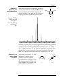
Example 1.
Synthesis of a
new triphosphine
An attempt to prepare compound 1 produced
a white solid with the 31P{1H} NMR spectrum
shown in Figure 1. Could this really be the
desired product? If so, what are the shifts and
coupling constant (needed for publication)?
PPh2
Ph2P
PPh2
1
Figure 1. 31P{1H}
NMR spectrum
(80.96 MHz;
1H = 200 MHz) of
phosphine 1?
-13.500
-14.500
-15.500
-16.500
-17.500
-18.500
-19.500
-20.500
Simulation quickly shows that this spectrum can indeed be explained
completely by a strongly coupled A2B system with δA = -17.5 ppm,
δB = -16 ppm, and JAB = 120 Hz. Without simulation, you might have
thought that you had a mixture of several compounds. Note that
there are no peaks in this spectrum with a separation of 120 Hz!
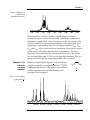
Example 2. cis
and/or trans
isomers?
An attempt to prepare 1,1,1,4,4,4hexafluoro-2-butene gave a
product with the 1H NMR
spectrum shown in Figure 2. Did
the synthesis succeed? And if so,
is the product the cis-isomer, the
trans-isomer or a mixture?
2
F
F
F
F
F
F
F F
F
F
F
cis
F
trans
Simulation and spectrum analysis
Chapter 1
Figure 2. Mixture of
cis and trans
hexafluorobutenes?
6.500
6.400
6.300
6.200
6.100
6.000
5.900
5.800
5.700
Both isomers are AA'X3X'3 systems, which always give rise to
symmetrical spectra. Since the spectrum contains two symmetrical
multiplets, it seems likely that it is a mixture of the two isomers. But
which is which? Even though the multiplets look complicated, their
appearance is governed by only four coupling constants: 2JHH, 3JHF,
4J
5
HF and JFF. A bit of trial-and-error simulation, followed by iterative
optimization, will yield values for all four parameters. The most
important one is probably JHH, which turns out to be 11 Hz for the
low-field multiplet, and 15.5 Hz for the high-field multiplet. This is a
strong indication that the major component is the cis isomer.
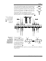
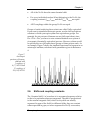
Example 3. An
unknown
rhodium
complex.
Reaction of diphosphine ligand 2 with a rhodium
complex resulted in a compound with the 31P{1H}
NMR spectrum shown in Figure 3. Is it possible to
deduce anything about the stoichiometry and
structure of the complex?
R2P
PR'2
2
Figure 3.Rh complex
of phosphine 2?
190.000 185.000 180.000 175.000 170.000 165.000 160.000
Simulation and spectrum analysis
3
Chapter 1
A few trial simulations show that the spectrum can
be explained by an AA'BB'X system (with X = Rh),
and accurate coupling constants can be obtained by
iteration (see Figure 4). Attempts to reproduce the
spectrum using A2B2X or AA'BB'XX' systems were
unsuccessful. This, in combination with the
numerical values of the coupling constants, shows
that the product is a cis bis(diphosphine) complex 2a.
R2P
PR'2
Rh
R2P
PR'2
2a
Figure 4. Observed
and simulated
spectrum of complex
2a, and parameters
used in the
simulation.
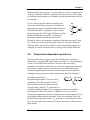
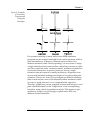
Example 4.
Dynamic
behaviour of
1,6;8,13-antibis(methano)[14]annulene.
H
H
H
H
Compound 3 has a
temperature-dependent
NMR spectrum (Figure
5).1 It seems reasonable
to explain this behavior
by "freezing out" of the
H
H
H
H
double-bond shift in 3
3
at low temperature. Is
this explanation correct, and if so, can we extract the rates at different
temperatures?
4
Simulation and spectrum analysis
Chapter 1
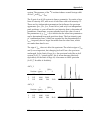
Figure 5.
Temperaturedependent spectrum
of annulene 3.
Simulation can be used to predict the appearance of the spectrum at
different exchange rates, given the parameters for the nonexchanging system. The results show that the proposed process is
indeed consistent with the observed spectra. Fitting produces the
rates at different temperatures, from which the activation parameters
can be deduced.
These examples demonstrate the usefulness of simulation in the
analysis of NMR spectra. Simulation is by no means necessary for
every analysis. But if you are uncertain whether a spectrum you have
measured may really correspond to a particular structure, simulation
can be an easy way of obtaining confirmation.
Simulation and spectrum analysis
5
Chapter 1
1.2.
Overview
The remainder of this manual provides some background on the
simulation of NMR spectra. It is not a textbook on NMR; if you do
not understand the principles of NMR, you should consult a textbook
before trying to read further. However, most of the aspects of NMR
spectroscopy that are relevant to simulation will be touched upon.
Chapter 2 discusses the "spin system", the basic unit that determines
the type of NMR spectrum. Chapter 3 then describes how a spectrum
can be calculated from this basic information. Chapter 4 touches
briefly on the prediction of spectral parameters from molecular
structures. Chapter 5 gives hints on how to simulate spectra of large
molecules. Chapter 6 explains what happens when the system being
studied is undergoing chemical reactions on the NMR time-scale.
Chapters 7 and 8 discusses the two iterative methods for obtaining
accurate parameters from experimental spectra, and chapter 9
describes the error analysis applicable to both.
Simulation is generally only useful when you already have an
experimental spectrum. Nowadays, NMR data are always recorded
as FID signals. This means that they have to be processed in some
way to convert them to a spectrum meaningful to humans. At the
very least, this requires a Fourier transformation; apodization,
resolution enhancement and corrections for various filters may also
be needed. Data processing is described briefly in Chapter 10. Finally,
we have collected in Appendix A a number of frequently
encountered second-order spectrum types that may help you in the
interpretation of your own spectra.
6
Simulation and spectrum analysis
Chapter 2
2.
The spin system
2.1.
Introduction
The information that is needed for an NMR simulation consists of a
qualitative part and a quantitative part. Together, they form the "spin
system.
The qualitative part is the "composition" of the system: the number
and types of NMR-active nuclei, and their symmetry relations. If the
structure of the molecule being studied is known, this part can
usually be written out easily. When the molecular structure is not
known, classification of the system is more difficult. In simple cases,
the type of spin system can be recognized directly from the NMR
spectrum (e.g., the distinctive pattern of an ethyl group, or the typical
6-line pattern of the X-part of an AA'X system). But most types of
spin systems have too many independent parameters to have a
distinctive, easily recognizable pattern. If you want to simulate a
complicated spectrum of a completely unknown compound, you will
often have to go through some trial and error as far as the type of
spin system is concerned.
The quantitative part is the set of shifts and coupling constants (and
possibly other relevant parameters like exchange rates). "Guessing"
accurate values for shifts and coupling constants is not easy (see also
chapter 4). But once you are close enough too see correspondences
between calculated and experimental spectra, further optimization
can usually be done by the computer.
It is important to note here that the appearance of the spectrum
depends only on the spectral parameters (shifts and couplings), not
directly on the structure. If two completely different chemical
structures would accidentally give rise to the same set of spectral
parameters, they would also produce the same NMR spectrum.
The spin system
7
Chapter 2
2.2.
Magnetic equivalence
The concepts of magnetic and chemical equivalence are very
important in NMR. Therefore, we will start with a formal definition
of magnetic equivalence, and then use a few examples to illustrate
the concept.
A group of two or more nuclei N1-Nn are called magnetically
equivalent if and only if:
•
All of the nuclei have the same chemical shift.
•
For every individual nucleus M not belonging to the set N1-Nn,
the coupling constants JN1M..JNnM are equal. However, different
couplings within the set are allowed, e.g. JN1N2 ≠ JN1N3.
In principle, such a situation could occur by chance, but the term
magnetic equivalence is usually reserved for those cases where there
is a symmetry reason for the above conditions to hold. Let us
consider two examples: sulfur tetrafluoride and o-dichlorobenzene.
F1
SF4 has a trigonal-bipyramidal structure, with one
F4
equatorial position occupied by a lone-pair orbital. As a
S
F3
consequence, it has two types of fluorine atoms: apical (1
F2
and 2) and equatorial (3 and 4). The two apical fluorines
have the same chemical shift (δ1 ≡ δ2), as do the
equatorial ones (δ3 ≡ δ4), but δ1 will be different from δ3. Also by
symmetry, all coupling constants between an apical and an equatorial
fluorine are identical. Therefore, there are two groups of magnetically
equivalent nuclei: the group of apical fluorines and the group of
equatorial fluorines. This spin system is called an A2B2-system.
Generally, a group of magnetically equivalent nuclei in a spin system
(e.g. the group of two apical fluorines) is denoted by a capital letter
(A) and a subscript (2) indicating the size of the group.2
8
The spin system
Chapter 2
H1
o-Dichlorobenzene (ODCB) also has two groups of
nuclei with identical chemical shifts: two ortho to a
H2
Cl
chlorine (1 and 4) and two para to a chlorine (2 and
3). However, nucleus 1 cannot be magnetically
Cl
H3
equivalent with 4, since J12 (an ortho-coupling)
H4
differs from J24 (a meta-coupling). It is not relevant
here that J12 ≡ J34 and J13 ≡ J24: as long as there is a
single nucleus i for which J1i ≠ J4i, nuclei 1 and 4 cannot be
magnetically equivalent. They are, however, called "chemically
equivalent", as explained below. The ODCB-type spin system is
usually called an AA'BB' or [AB]2 system. Inequivalent nuclei that
are related by a symmetry operation are usually indicated by a
notation using primes, e.g. AA' for hydrogens 1 and 4. Note that the
overall molecular symmetry of SF4 and ODCB is the same, C2v,3 so
overall symmetry is not enough to determine magnetic equivalence.
We will not discuss symmetry notations in detail here; for
an excellent discussion, see Reference 3. C2v indicates the
presence of two mirror planes and a twofold axis, Cs means
just a single mirror plane, and C1 means no symmetry at
all.
Magnetic equivalence is important because it allows considerable
simplification in the calculation of NMR spectra. One of the reasons
for this is a theorem which states that for any group of magnetically
equivalent nuclei in a system, couplings within the group do not
affect the spectrum and can be ignored. This means less typing for
you, since you do not have to enter them. It can also be a
disadvantage, since these constants cannot be determined from the
experimental spectrum unless you reduce the symmetry of the
molecule (e.g., by isotopic substitution). For example, the SF4
spectrum is completely determined by two shifts (δ1 and δ3) and one
coupling constant (J13); J12 and J34 do not affect the spectrum and
cannot be determined. In contrast, there are six relevant parameters
in the ODCB system (δ1, δ2, J12, J13, J14 and J23), and they can all be
determined from the observed spectrum. The greater complexity of
the AA'BB'-system is clearly illustrated in Figure 6.
The spin system
9
Chapter 2
Figure 6. Spectra of
SF4 (left) and odichlorobenzene
(right).
2.3.
Chemical equivalence
Two or more nuclei are called "chemically equivalent" when they
have the same chemical shift for reasons of symmetry. The values of
coupling constants are not relevant to this definition, but the
symmetry will in general imply some relationship between coupling
constants involving chemically equivalent nuclei. Magnetic
equivalence implies chemical equivalence, but not vice versa.
As an example, consider the four protons in the ODCB molecule
discussed in the previous section. The molecule has C2v symmetry,
which causes H1 and H4 to have the same chemical shift (the same
holds for H2 and H3). Thus, ODCB contains two groups of
chemically, but not magnetically, equivalent protons. The molecular
symmetry also implies that J13 ≡ J24 and J14 ≡ J23.
The use of chemical equivalence (or symmetry in general) in NMR
simulation can significantly reduce the computation involved.
However, the full exploitation of symmetry is less trivial than that of
magnetic equivalence, so not all simulation programs use full
symmetry factorization.
If nuclei are magnetically equivalent, they can be specified in groups,
since they all have the same coupling constants to nuclei outside the
group. Thus, you only have to specify a single entry for each
magnetic-equivalence group instead of for each individual nucleus.
Such a simplification is not possible for chemical equivalence, since
different nuclei in a chemical-equivalence group may have different
coupling constants to a single nucleus outside the group. Therefore,
you will have to supply a separate entry for each nucleus in a
10
The spin system
Chapter 2
chemical-equivalence group. You can, however, enforce symmetry by
"linking" parameters (shifts, coupling constants) to ensure that, when
you change one parameter, all symmetry-related parameters will also
be changed.
Me
It is not always trivial to decide whether two
'
H
2
nuclei are chemically equivalent. Consider the
O
H1'
methylene groups of acetaldehyde diethylacetal.
H
H
This molecule has Cs symmetry, with a mirror
Me
H1 2
O
plane bisecting the OCO angle. Reflection in this
Me
plane interchanges H1 and H1', so these two
hydrogens must be chemically equivalent.
However, there is no symmetry operation that interconverts H1 and
H2. These protons are diastereotopic. They not only have different
chemical shifts, but will also differ in other chemical properties (for
example, the rates of abstraction by a strong base will be different).
2.4.
Temperature-dependent equivalence
The above discussion suggests that the classification of nuclei as
chemically or magnetically equivalent is absolute, i.e. only dependent
on the overall molecular structure. However, there are many
examples of molecules which have a static low-temperature structure
but acquire a higher effective symmetry at elevated temperature,
usually through rapid inversion or rotation processes or chemical
exchange (rate processes are discussed in more detail in chapter 6).
6
6'
Consider a molecule of
dicyclohexylphosphine. This has only Cs
2
2'
P
symmetry; the carbon atoms 2 and 6 of
each cyclohexyl ring are diastereotopic
H
(inequivalent), and the 13C spectrum of a
carefully purified sample at low temperature shows two distinct
resonances for these two carbons. Addition of a trace of acid or
raising the temperature results in rapid inversion at phosphorus via a
protonation-deprotonation pathway. In the fast-exchange limit, the
molecule has acquired effective C2v symmetry; carbon atoms 2 and 6
have become equivalent, and only a single resonance is observed for
these atoms.
The spin system
11
Chapter 2
A simpler example is the methyl group of an ethyl compound. In any
static structure, it can have at most Cs symmetry, which would give
rise to two separate resonances in the ratio 2:1. However, the barrier
to methyl rotation is usually extremely low (<4 kcal/mol), so the
rapid rotation occurring under most terrestrial conditions results in
effective magnetic equivalence of the three methyl protons. Similarly,
the three methyl groups of a t-butyl or trimethylsilyl group are
usually equivalent.
2.5.
Anisotropic spectra and full equivalence
So far, we have assumed that coupling constants are simply numbers.
In fact, they are tensors and have an orientation-dependent term. In
non-viscous solutions, however, the molecules tumble rapidly and
have no preferred orientation, so we only see the average over all
orientations (the "trace") of the coupling tensor, which is the number
we call the (indirect) coupling constant J.
It is also possible to record NMR spectra of compounds dissolved in
liquid crystals ("anisotropic media", hence the term "anisotropic
spectra"). In such a medium, the molecules will not tumble
completely randomly, but will have a preferred orientation with
respect to the medium and to the external field. Because of this, the
averaging of the coupling tensor is incomplete, and we also see a
contribution of a second coupling, called the direct or dipolar
coupling D. Dipolar couplings are usually much larger than indirect
couplings. Because they provide information on the spatial positions
of atoms, analysis of anisotropic spectra can yield direct structural
information. This is a rather specialized topic: see Reference 4 for a
more detailed discussion. To simulate anisotropic spectra, you will
have to supply direct (D) as well as indirect (J) coupling constants; if
possible, you should extract the indirect couplings from isotropic
spectra and fix them in anisotropic calculations.
In our discussion of magnetic equivalence earlier in this Chapter, we
stated that couplings within a magnetic-equivalence group do not
affect the spectrum. This is no longer true for anisotropic spectra. The
indirect couplings J within the group are irrelevant, but the direct
couplings D do contribute to the spectrum and must be included in
the simulation. So, for anisotropic spectra the rules for equivalence
are stricter:
12
The spin system
Chapter 2
•
All of the N1-Nn have the same chemical shift.
•
For every individual nucleus M not belonging to the N1-Nn, the
coupling constants JN1M..JNnM and the DN1M..DNnM are equal.
•
All D couplings within the group N1-Nn are equal.
Groups of nuclei satisfying these criteria are called "fully equivalent".
If you want to simulate anisotropic spectra, use the full-equivalence
criterion to divide your spin system into equivalence groups. For
example, the six protons of benzene are not fully equivalent, since
D12 ≠ D13 ≠ D14: you have to enter oriented benzene as a system of
six separate (chemically equivalent) protons. However, ethane could
be specified as two full-equivalence groups of three protons each. As
an example, Figure 7 shows the simulated spectrum for benzene in an
anisotropic medium, calculated with parameters given in Reference
4.
Figure 7.
Anisotropic
spectrum of benzene,
obtained with
J couplings of
8 / 2 / 0.5 Hz and
D couplings of
333 / 64 / 42 Hz.
2.6.
Shifts and coupling constants
The "chemical shift" δ of a nucleus is its resonance frequency relative
to that of a particular reference compound. The shift is proportional
to the external magnetic field, which is why shifts are usually
expressed in ppm of the field: for different fields, they are constant
when expressed in ppm, not when expressed in Hz. By convention,
The spin system
13
Chapter 2
the sign of δ is chosen in such a way that higher δ values correspond
to higher resonance frequencies. Also by convention, NMR spectra
are written with δ values increasing from right to left.
In principle, the chemical shift is a tensor, but in liquid NMR
one usually just observes its trace, which is a scalar or
number.
The magnitudes of chemical shifts are often discussed using a
number of different terms, which correspond as follows:
low δ value
high δ value
low frequency
high frequency
high field
low field
high shielding
low shielding
shielded
deshielded
diamagnetic shift
paramagnetic shift
The "coupling constant" between two nuclei A and B is the energy
difference between the situations where the two nuclei have parallel
and antiparallel spins. More precisely, the energy contribution to the
Hamiltonian is5
EAB = h JAB mI(A) mI(B)
From this equation, it is apparent that J > 0 implies the situation with
parallel spins is higher in energy than the one with antiparallel spins.
The energy difference is independent of the external field, so
couplings are expressed in Hz. It is important to realize that (in
contrast to e.g. infrared force constants) there is no general
connection between coupling constants and bond strengths.
Shifts and couplings can usually be regarded as molecular properties.
They are somewhat sensitive to temperature and solvent, but
variations caused by the environment are usually small compared to
the differences between different molecules. The most notable
exceptions are observed for the chemical shifts of protons involved in
hydrogen bridges.
Both chemical shifts and couplings can also usually be related to the
direct environment (1-3 bonds) of the nucleus or pair of nuclei in
question. In that sense, they are local probes of chemical structure.
14
The spin system
Chapter 2
Particular orientations of bonds or π-systems relative to a nucleus can
cause longer-range effects on chemical shifts, and particular shapes of
the bond path connecting two nuclei sometimes result in abnormally
large long-range couplings. The prediction of NMR parameters from
molecular structures is discussed briefly chapter 4.
2.7.
The signs of coupling constants
NMR resonances are due to transitions between different spin states
of nuclei. Coupling constants are a measure of the influence that the
spin state of one nucleus has on the energy levels of another nucleus.
A positive coupling constant implies that the nuclei prefer to have
their spins antiparallel (αβ or βα), and a negative coupling constant
implies that they prefer to have their spins parallel (αα or ββ).5
In general, it is difficult to determine the absolute sign of a coupling
constant, but relative signs (i.e., relative to the signs of other coupling
constants) can often be determined by several types of 1-D or 2-D
experiments. It is possible to give rules for the signs of some types of
coupling constants. For example, the geminal coupling of an aliphatic
methylene group is usually negative; vicinal HCCH couplings are
nearly always positive. For other types of couplings, however, the
signs can vary from compound to compound.
If coupling constants can have either sign, the question arises
whether these signs affect the appearance of the NMR spectrum. In
general, spectra that are completely first-order are not affected by the
signs of coupling constants. However, sign changes affect the peak
labeling, which may be important in iteration. In spectra showing
second-order effects, signs may be important. It is often true that
there are groups of coupling constants which can change signs
simultaneously without affecting the spectrum, whereas individual
sign changes may produce a different spectrum. Before reporting the
results of an iteration, it is important to check how many alternative
sign combinations would also produce an acceptable (possibly
identical) solution.
The spin system
15
Chapter 2
2.8.
Isotopic substitution
Molecules of the same chemical composition but having a different
isotopic composition are usually called isotopomers. The presence of
different isotopes of a single element can give rise to a number of
interesting effects in NMR spectroscopy.
To a very crude first approximation, the presence of an isotope does
not disturb the shifts and coupling constants of the other nuclei in the
molecule.
This is really a rather crude approximation. Especially for
nearest neighbors, the effect is often significant. Typical
one-bond isotope shifts ∆δ are -0.5 ppm in 13C for CH→CD
and -0.03 ppm in 31P for P12C→P13C.
Also, the chemical shift of the isotope (expressed in ppm) will be
approximately the same as that of the original nucleus in the original
molecule, and coupling constants JXY of any nucleus X to the isotope
Y are related to the original coupling constants JXZ via
JXY/JXZ ≈ γY/γZ. These relationships between isotopomers are not
exact, because the presence of an isotope changes the vibrational
levels of a molecule and the populations of different conformers.
Obviously, substitution of a single isotopic nucleus for one member
of a magnetic-equivalence group destroys the equivalence. Couplings
to the isotope can now be observed, and the above relationship can
be used to estimate the coupling constants within the original group
of equivalent nuclei. For example, substitution of one proton of a
methyl group by deuterium allows observation of 2JHD and therefore
estimation of 2JHH of the original methyl group as 2JHH ≈ 6.5×2JHD.
The presence of an isotope can also destroy the symmetry of a
molecule in a more subtle way. For example, ethylene has four
equivalent 1H atoms, and the 1H NMR spectrum shows just a singlet:
no H-H coupling constants can be extracted. However, the presence
of a single 13C atom in this molecule lowers the symmetry and
produces an AA'BB'X-type spectrum, from which all H-H and C-H
coupling constants can be determined.
16
The spin system
Chapter 2
C1
C3
Symmetry reduction is particularly
Ph
P
C
PPh2
13
2
2
important in natural-abundance C
spectroscopy, when one usually looks at
molecules having a single 13C atom. Even if the original (all-12C)
molecule is symmetrical, many of its 13C-isotopomers will not be
symmetrical because the 13C atom does not lie on all symmetry
elements. This has noticeable consequences, particularly if there are
other magnetically active nuclei in the molecule. For example,
consider the diphosphine 1,3-bis(diphenylphosphino)propane and its
1-13C and 2-13C isotopomers. In the all-12C species, the phosphorus
atoms are equivalent. They are also equivalent in the 2-13C
isotopomer, and the 13C resonance of C2 will be a nice triplet. In the
1-13C isotopomer, however, the phosphorus atoms are inequivalent,
since the 13C atom destroys the symmetry. The 1JPC coupling
constant will be different from 3JPC, and there will also be a small
shift difference between the two phosphorus atoms. Therefore, the
13C peak for C will have a more complex splitting pattern. Very
1
complex patterns can also be observed in 1H-coupled 13C spectra of
symmetrical molecules.
The spin system
17
Chapter 3
3.
Simple simulation
3.1.
Linewidths and lineshapes
In the case of a single nucleus resonating at a So far, we have been
discussing NMR spectra as if they were "stick" spectra, that could be
fully characterized by a set of peak positions and intensities.
Actually, peaks also have a particular lineshape.
frequency f0 with a relaxation behavior characterized by a single
transverse relaxation time T2, in the absence of saturation, the
absorption lineshape is a pure Lorentzian with a width at half-height
of W½ = (πT2)-1:
S( f ) ∝
W
2
 W
2
  + ( f − f0 )
 2
In practice, however, ideal relaxation behavior is seldom observed.
The actual linewidth is often dominated by field inhomogeneities, in
which case the lineshape tends to resemble a Gaussian
 f − f0

W 
1 − 2
S( f ) ∝ e 
W
2
Even under idealized conditions, both lineshape functions are strictly
applicable only to either CW scans or to FT spectra without
weighting. In practice, cleverly chosen weighting schemes are widely
used to improve the appearance of NMR spectra, and such weighting
may occasionally produce bizarre results, including lines complete
with fake wiggles! Imperfect phasing may result in mix-in of
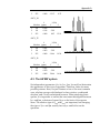
dispersion components of the lineshape functions. Typical absorption
and dispersion lineshapes (Lorentzian, Gaussian and triangular) are
illustrated in Figure 8. In particular, note the extremely slow fall-off
of the dispersion component of a Lorentzian away from its centre.
Simple simulation
19
Chapter 3
Figure 8. Examples
of Lorentzian,
Gaussian and
Triangular
lineshapes.
For systems consisting of many nuclei, most NMR simulation
programs use just a single linewidth for the whole spectrum, which is
often unsatisfactory. In practice, different nuclei can have very
different relaxation times. Strictly speaking, it is not correct to assign
a single relaxation time to each nucleus: relaxation processes of nuclei
are often connected, and a "relaxation matrix" treatment is needed for
an accurate description. In practice, however, having a single
relaxation time per nucleus is usually satisfactory; exceptions occur
in cases with chemical exchange (see chapter 6) or with quadrupolar
relaxation. There is no "clean" way of assigning a different relaxation
time to each nucleus, short of the relaxation matrix treatment, which
we want to avoid because it is too computationally expensive.
Therefore, gNMR uses a more pragmatic solution and assigns to each
peak a linewidth based on the "composition" of the corresponding
transition, using a kind of population analysis. This appears to give
satisfactory results even for strongly coupled nuclei with very
different natural linewidths.
20
Simple simulation
Chapter 3
3.2.
First-order spectra
In simple cases, the appearance of an NMR spectrum can be
predicted easily using the following rules:
•
Every nucleus has a peak at its "resonance frequency", given by
the chemical shift δ. The area of the peak is proportional to the
number of nuclei.
•
For every pair of (spin-½) nuclei between a coupling exists, both
peaks are split into two components, with the same splitting J.
If one of the nuclei has a spin I different from ½, it splits up
the other peak into 2I+1 components.
Repeated application of these rules produces the familiar doublets,
triplets, quartets etc. of high-resolution liquid NMR spectroscopy. If
the nuclei are all of different types (e.g., 1H and 31P) these rules are
virtually exact. For molecules containing several nuclei of the same
type, small deviations are usually observed (mostly intensity
changes).
Cl
Spectra that are (nearly) first-order are best
interpreted "by hand". Chemical shifts are assigned
from the centers of multiplets, and J couplings from
N
the splittings. Comparison of splittings in different
multiplets can be used to assign couplings to a specific
pair of nuclei; small "thatch" effects may also be helpful here. As an
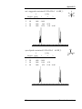
example, Figure 9 shows the first-order analysis of the 1H spectrum
of 2-i-propyl-3-chloro-pyridine.
In principle, this process could be automated. However, analysis
programs get confused easily by partially overlapping lines in
multiplets, and they also have a tendency to miss the weak outer
lines of e.g. septets, which makes such automatic analysis unreliable.
Simulation is generally not needed to analyze simple first-order
spectra. In fact, the time required to set up the simulation may well
exceed that needed to interpret the spectrum by hand.
Simple simulation
21
Chapter 3
Figure 9. First-order
analysis of 1H NMR
spectrum of 2-ipropyl-3-chloropyridine.
3.3.
Second-order effects
Second-order effects are all deviations from the simple rules for
spectrum appearance mentioned above. The use of higher field
strengths is often cited as the remedy for all second-order effects in
NMR. Chemical-shift differences become large compared to coupling
constants, so second-order effects will surely disappear. While this is
an attractive argument for buying higher-frequency spectrometers,
and for avoiding delving into NMR simulation, it is incorrect.
As a general rule, you will see second-order effects when the
chemical-shift difference between two nuclei is of the same order of
magnitude as the coupling constant between them (say, to within a
factor of 10 either way). If the coupling constant is very small, the
nuclei are "weakly coupled" and will give rise to a simple first-order
spectrum. If the coupling constant is very large, the nuclei become
effectively equivalent, again giving rise to a first-order spectrum.
Second-order effects are expected in the intermediate range of
"strong coupling". The first signs of second-order effects are usually
22
Simple simulation
Chapter 3
small intensity distortions: inner lines become more intense at the
expense of outer lines. If the coupling becomes stronger, the
distortions become larger and extra splittings may appear. Also,
second-order effects may appear on the multiplets of other nuclei in
the molecule, even though these are not strongly coupled to any spin
in the molecule.
If two nuclei are magnetically equivalent, you can treat them as a
group: second-order effects will appear when coupling constants to
nuclei outside the group become comparable to chemical-shift
differences between these nuclei. Thus, the second-order effects in an
A2B3 ethyl group depend on the ratio JAB/∆δAB; both JAA and JBB are
irrelevant.
If there are groups of chemically equivalent nuclei in the molecule,
you can expect problems. The shift difference between the nuclei in
the group is zero by symmetry, so there is no J/∆δ rule to use.
Instead, you can expect second-order effects when, for any nucleus X
outside the group and two nuclei Y and Z inside the group, the ratio
rX = JYZ/JXY-JXZ is in the order of 1. If rX is very small, you will see
separate XY and XZ coupling constants; if rX is very large, you will
only see an average "virtual" coupling, and if rX ≈ 1 you will see
second-order complications. You can also expect second-order effects
if rX is very small for some X and very large for others, even if there
is no X for which rX ≈ 1.
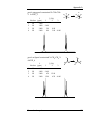
To illustrate this, Figure 10 shows the 1H spectrum of ODCB at
different magnetic-field strengths. At low field, the inner lines are
much more intense than the outer lines: this second-order effect is
caused by the small chemical-shift difference between the two types
of protons. For fields higher than ca 300 MHz, this effect has largely
disappeared: the two multiplets are each approximately symmetrical.
However, they are not simple doublets of doublets of doublets, and
will not become so at any field: the small outer lines of each multiplet
really belong to the spectrum and will not disappear. The criterion
for second-order effects here, r1 = J23/J12-J13 = 7.47/(8.14-1.49) ≈ 1,
is fulfilled regardless of the external field. Therefore, interpretation of
the splittings as coupling constants is not allowed, and will in fact
produce completely incorrect values.
Simple simulation
23
Chapter 3
Figure 10.
Calculated spectra of
ODCB at different
field strengths.
There is nothing mysterious about second-order effects. Their origin
is completely understood, and any decent simulation program will
produce the correct spectrum given the right parameters. However,
interpretation of second-order spectra without a simulation program
is difficult, since the human mind and eye are simply not well suited
to the recognition of patterns of matrix eigenvalues. Therefore,
simulation is an indispensable tool for the interpretation of secondorder spectra.
24
Simple simulation
Chapter 4
4. Prediction of parameters from
molecular structure
It would be nice if it were possible to predict chemical shifts and
coupling constants from a given molecular structure. Unfortunately,
this is not generally possible at present, although some significant
advances have been made in recent years. There are two different
ways to approach the problem: empirical methods (based on
measured data) and theoretical methods (based on quantumchemical calculations).
•
Empirical methods
Using a database containing many known compounds with their
NMR data, it is possible to estimate data for related but unknown
compounds using various statistical methods and structureproperty relationships. The accuracy of this method depends
strongly on the quality and size of the set of reference data.
Clearly, it is impossible to predict data for compounds with very
abnormal structures or interactions in this way. Accurate
prediction is now possible for 1H and 13C shifts and couplings of
"normal" organic compounds, and database-based prediction
programs for 19F and 31P have recently started to appear.
Predictions of metal NMR shifts is not yet available, partly
because of the lack of sufficient reference data and partly because
there is not enough (commercial) interest.
•
Theoretical methods
Ab initio calculation of coupling constants is possible but requires
large basis sets and advanced electron correlation treatments.
Chemical shifts can be calculated with reasonable accuracy (a few
ppm for heavy atoms, or ≈0.5 ppm for hydrogen), but this
requires the use of optimized structures and polarized basis sets.
These calculations are therefore mostly limited to simple
molecules, with up to ca 15 non-hydrogen atoms. However, the
method allows predictions for exotic structures as well as for
"normal" organic molecules.
At least as important as the computational problems of the
theoretical approach are the chemical ones. NMR parameters are
the time-averaged values over all accessible conformations of a
molecule, and often also include significant contributions due to
Parameters and structure
25
Chapter 4
interaction with the solvent. Therefore, accurate prediction from
theory alone is at least an order of magnitude more complicated
than just a single IGLO or GIAO calculation.
As an alternative to the rather expensive ab-initio method,
prediction using semi-empirical methods has also been
attempted. Extensive parametrization is required to make this
work, including classification of "atom types". Therefore, this
method, is again unsuitable for unusual bonding situations or
non-standard nuclei. However, it may be a useful addition to the
database approach mentioned above.
If one doesn't set the sights too high, simple additivity rules for
chemical shifts can produce quite reasonable results. We have found
the rules given by Pretsch6 quite useful, but other good collections
exist. Coupling constants are strongly conformation dependent, but
for most common cases this dependence is well documented (if not
completely understood), so if the 3D structure of a molecule is
known (short-range) couplings can be estimated with reasonable
accuracy. Abnormally large long-range couplings are nearly always
associated with particular geometries of the bond path ("zigzag" or W
paths), or with very short through-space contacts; prediction of the
magnitude of such couplings is difficult.
26
Parameters and structure
Chapter 5
5.
Simulating large systems
5.1.
On the scaling of NMR calculations
In principle NMR simulation is simple. Set up the Hamiltonian,
diagonalize to get the energy levels, multiply eigenvectors with
transition moments to get intensities, evaluate a Lorentzian for every
calculated peak...
Unfortunately, the scaling of the calculation is rather unpleasant. The
size of the calculation (dimension of the Hamiltonian) scales as
 n / 2
n-2, the storage requirements as the square of this, and the

 ≈ 2
 n 
computing time as its cube. For every nucleus added to the system,
the time required increases with a factor of 8! This makes calculations
for large molecules (> 12-15 atoms) rather difficult. For example, on a
100 MHz Pentium a particular 6-spin problem took 0.1 seconds to
simulate, an analogous 8-spin problem 0.73 seconds, the 10-spin
problem 22 seconds, and the 12-spin problem 27 minutes. With the
current rates of increase of CPU speed (a factor of 2 every 1-2 years),
it will be several decades before we can do 25-spin systems! This is
the reason many NMR simulation programs won't let you simulate
systems larger than 8 spins. Or if they do, the spectrum is often
evaluated by first-order methods, which are rarely good enough.
There are several methods for reducing the computation
requirements of a simulation. Some of these can be carried out
automatically by the simulation program, and some can be done by
the user, as detailed in the next two sections. But none of these will
help with the simulation of really large systems (say, larger than 15
nuclei). To handle such systems, one must resort to approximate
calculations, and that is the topic of the final section of this chapter.
5.2.
Simplification by the simulation program
The following techniques can be applied automatically to reduce the
size of an NMR simulation without any loss of accuracy:
•
Splitting of the system into uncoupled fragments if possible.
Large systems
27
Chapter 5
•
Detection of magnetic equivalence, and treating of groups of
magnetically equivalent nuclei as composite particles.
•
Detection and use of full molecular symmetry (chemical
equivalence).
•
Division of the system into "X-groups" for nuclei of different
types.
Splitting a system can result in huge savings of computation time.
The other techniques will only result in a modest reduction of the
size of the calculation. Nevertheless, it is worthwhile to exploit them
whenever possible.
If the result need not be exact (but still rather good), it is possible to
use the technique of "X-group" division between nuclei of the same
type. This will introduce errors, but as long as the groups are only
weakly coupled most errors can be eliminated by the use of
perturbation theory to handle the interaction between these groups.
Perturbation theory does not result in large savings, but - like the
other techniques mentioned above - it can make the difference
between a feasible simulation and an impossible one.
5.3.
Simplification by the user
Unlike a simulation program, you as user know what is really
interesting about a particular spectrum. Therefore, you can take more
drastic measures to reduce the size of a simulation:
•
Delete parts of the molecule remote to the fragment of interest.
•
If you are interested in a molecule having several equivalent
fragments, use only one such fragment and if necessary
"terminate" it with an innocent end-group.
•
Set very small couplings between nuclei in different fragments to
zero, so that the simulation program can divide the molecule into
uncoupled fragments.
These measures will all change the simulated spectrum, unlike the
ones mentioned in the previous section. Therefore, it would be
28
Large systems
Chapter 5
unwise to let the program apply them automatically. And if you
apply them yourself, you should always try to check whether the
simplifications were justified. For the correct simulation of secondorder systems, you often need to include more than just the nuclei
that couple directly to the fragment of interest.
Ph
As an example, let us try to reproduce the Ph CH2
CH2
methylene group signals of a
P Rh P
bis(benzylphosphine)rhodium complex
Ph
Ph
(Figure 11A). The two protons of each
Py
Py
methylene group are diastereotopic, so we
will need at least these two protons, a phosphorus atom, and the
rhodium atom (the Rh-H couplings are not zero). This gives a 4-spin
H2PRh system. However, even the best simulation (Figure 11B)
comes nowhere near the experimental result.
The 2JPP coupling is fairly large (43 Hz), so we may have to include
the second phosphorus atom. In that case, we will also have to
include the second CH2 group. If we did not do so, the phosphorus
atoms would become very different, and the results might not be
meaningful. The system is now a 7-spin H4P2Rh system, already
rather large, but the simulation (Figure 11C) is still unable to
reproduce the curious pattern of the experimental spectrum,
although it starts to look reasonable. What can be missing here?
There are no significant couplings from the methylene group to the
benzylic phenyl group, so the problem must be somewhere else. It
turns out that extra couplings to the phosphorus atoms are needed to
get the pattern of Figure 11A. These couplings are really there: the
phenyl and pyridyl protons all have significant phosphorus
couplings. What is surprising is that you would need them to
reproduce the benzylic methylene signal. Luckily, you do not need all
the phenyl and pyridyl protons in the simulation. Figure 11D shows
the simulation of Figure 11C with just one hydrogen atom added per
phosphorus atom (JPH = 20 Hz). This is a 9-spin H6P4Rh system, near
the limit of what most simulation programs can handle, but the
pattern finally looks correct. Of course, the addition of a single P-H
coupling to represent the effect of one phenyl and one pyridyl ring
looks a bit like fudging. Clearly, any coupling constant fitted for it
will be meaningless, and some other parameters may not be very
significant either. However, the exercise illustrates that you really can
Large systems
29
Chapter 5
get the curious resonance shape of Figure 11A from the structure
shown above.
Figure 11.
Methylene
resonance of a bis(benzylphosphine)rhodium complex
(A), simulated with
increasingly
complicated spin
systems (B-D).
5.4.
Approximate calculations
As mentioned earlier, for really large molecules exact simulation is
impossible, so one is forced to resort to some sort of approximate
calculation. The most drastic approach is simple first-order
calculation (see section 3.2), possibly with some cosmetic corrections
to reproduce "thatch effects". This is certainly extremely fast, but is
only good for near-first-order spectra, for which one usually doesn't
need simulation anyway.
Here we propose an intermediate scheme based on a "divide-andconquer". It has been implemented in gNMR and appears to work
satisfactorily in most cases. We call this method 'chunking'.
The design of the algorithm is based on the way one normally does
the analysis of a spectrum. Whereas a simulation program calculates
the whole spectrum at once, a chemist will look at each individual
multiplet in turn. Direct couplings to the nucleus in question are
considered first (the "first shell"). If there are other nuclei that don't
couple directly with the target nucleus but do couple strongly to
other nuclei in the "first shell", second-order effects will occur (e.g.,
"virtual triplets"), and these nuclei are also required to understand
the spectrum (the "second shell"). One could go further, but in
30
Large systems
Chapter 5
practice two "shells" are usually sufficient to explain the shape of a
multiplet.
This suggests that the simulation should also calculate the multiplets
one by one, using only as much of the environment as is needed to
reproduce the patterns. The problem is that simulation of a part of a
molecule will not only produce the target multiplet (which is
presumably accurate), but also resonances due to the "shells", which
are probably very inaccurate. The key point of the approximate
approach is that the simulation is indeed done in chunks, but from
each chunk spectrum everything is thrown away that is not due to its
target nucleus; then the chunk spectra are added to give the final
spectrum. The technical details can become a bit complex but are not
important here.
The key advantage of this scheme is that it scales linearly in system
size, which means that future increases in CPU speed will
immediately result in the ability to simulate significantly larger
systems. The minimum chunk size needed to obtain correct multiplet
patterns is usually 8-9 nuclei, so the break-even point of this method
appears to be in the range of 11-12 nuclei. For smaller systems, exact
simulation is still the method of choice.
Large systems
31
Chapter 6
6.
Chemical exchange
6.1.
The effects of chemical exchange
In contrast to many other spectroscopic methods, where kinetics can
only be used to study irreversible reactions, NMR can also be used
for kinetic studies of systems in equilibrium. This is because the
NMR time-scale, of the order of milliseconds or microseconds, is
conveniently close to our own time-scale. Reversible processes with
activation energies of the order of 5-20 kcal/mol can be studied by
"band-shape analysis", explained below.7 For reactions with slightly
higher barriers, techniques like polarization transfer may be more
appropriate.
As an illustration of an exchange process, let us consider Me2NPF4,
which has been studied by Whitesides8 (We have modified a few
parameters from the data given by Whitesides to make the example
more illustrative). This has a trigonal-bipyramidal structure, with the
amino group in the equatorial plane. There are two groups of
magnetically equivalent fluorine atoms, as in the SF4 example
discussed earlier. Since the phosphorus atom is also magnetically
active, we can characterize this molecule as an A2B2X system
(ignoring the dimethylamino group). The low-temperature 31P
spectrum (a triplet of triplets, Figure 12A) can indeed be interpreted
in this way. However, at higher temperatures the fluorine atoms start
to exchange. In the high-temperature limiting spectrum (also called
the "fast-exchange limit"), the spectrum shows just the quintet of an
A4X system (Figure 12D): the fluorine atoms have become equivalent
"on the NMR time-scale". What happens is that the exchange is so
much faster than the actual NMR experiment that we observe the
time-averaged situation.
Chemical exchange
33
Chapter 6
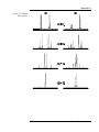
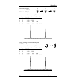
Figure 12. One-pair
(left) and two-pair
(right) exchange 31P
spectra for
Me2NPF4.
Neither the low-temperature (or "slow-exchange") limit nor the hightemperature limit is particularly interesting: the interesting things
happen in between. As the temperature is raised, the initially sharp
lines (Figure 12A) broaden and coalesce (Figure 12B, C) until, in the
fast-exchange limit, a sharp spectrum is obtained again (Figure 12D).
For the intermediate situations, it is possible to determine a rate
constant from the line broadening by fitting. The temperature
dependence of the rate constant can then be used to extract activation
34
Chemical exchange
Chapter 6
energies and entropies. Moreover, different exchange mechanisms
may give rise to different line broadening patterns in intermediate
situations, even though the fast-exchange limits are the same. If these
differences are large enough (as they are in Figure 12), it will be
possible to distinguish between such mechanisms; in the particular
case discussed here, the reaction was clearly shown to follow a twopair exchange pathway.
6.2.
Intra- and inter-molecular exchange
Actually, the terms intra- and inter-molecular exchange are slightly
misleading, because their normal chemical meaning is not entirely
appropriate to NMR. The distinctions needed to understand dynamic
behavior are more subtle. Four typical examples are illustrated
below.
H
CH3
We will start with the simplest case, which is often
called intramolecular mutual exchange, and will use
N
dimethylformamide as an example. The dynamic
O
CH3
behavior shown by this molecule (Figure 13A) is
hindered rotation around the amide bond. At low
temperature, you will see two different methyl resonances in the 1H
spectrum. On raising the temperature, they broaden and then
coalesce to a single peak. In effect, all six protons of the methyl
groups have become magnetically equivalent on the NMR time-scale.
The position of the single peak corresponds (approximately) to the
average of the chemical shifts of the individual methyl groups. If
there had been any observable couplings from the methyl groups to
other parts of the molecule, the high-temperature limit would also
show averages of these coupling constants. The Me2NPF4 example
discussed above also showed such an exchange in its 31P spectrum.
Chemical exchange
35
Chapter 6
Figure 13. Effect of
hindered C-N
rotation on (A)
HCON(CH3)2
and (B)
HCON(R1)(R2).
36
Chemical exchange
Chapter 6
H
CH3
H
C*H3
Now consider the 13C
spectrum of the same
C N
C N
compound. At low
O
CH3
C*H3
temperature, we actually have O
two different "molecules": one
with a 13C atom trans to oxygen, and one with the 13C atom cis to
oxygen. (We are ignoring molecules containing two or more 13C
atoms because their abundance will be negligible). This type of
exchange is called intramolecular non-mutual exchange. For this
particular case, the resulting spectrum will still be rather similar to
the 1H example described above, but the distinction between mutual
exchange (within a single species) and non-mutual exchange
(exchange of species) is important.
R1
H
R2
We can carry this point further by H
looking at the isomerization of an
C* N
C* N
amide with different organic
R1
O
O
R2
groups at the nitrogen. Let us
consider only the 13C resonance of
the carbonyl carbon. Since the two organic groups in our hypothetical
amide are different in size, there will be an energy difference between
the cis- and trans-isomers: the equilibrium will contain (say) 10% cis
and 90% trans.
Figure 13B shows the (simulated) behavior. Note that, at equilibrium,
the forward and backward reaction rates are equal. This implies that
the rate constant of disappearance of the cis isomer,
kcis→trans = Rate/[cis], is much larger than the rate constant of
disappearance of the trans isomer, ktrans→cis = Rate/[trans]. Therefore,
line broadening for the cis isomer starts at a lower temperature than
for the trans isomer: the process does not look very symmetric. The
high-temperature effective chemical shift is an average (weighted by
the concentrations) of the separate low-temperature chemical shifts; if
there were any coupling constants, these would become weighted
averages as well.
Finally, we will consider an example of what is commonly called
intermolecular exchange, using a hypothetical metal-bis(phosphine)
complex as an example.
Chemical exchange
37
Chapter 6
P
P'
+
M
P
C
P'
M'
+ M'
M
P'
C'
P
P
C
P'
C'
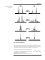
This example, which shows a curious rate dependence of the NMR
signal, was first described by Swift (Reference 9). Figure 14 shows the
theoretical 13C resonance of a carbon atom of the phosphine ligand as
a function of the exchange rate of the phosphines.
At low exchange rates, the spectrum is a virtual triplet, because JPP is
large. At high exchange rates, the 13C atom only "sees" the
phosphorus atom in its own ligand molecule, so the spectrum is a
nice doublet. At intermediate exchange rates, something curious
happens: it looks as if there is only a (broad) singlet! Not all
intermolecular exchange processes show such strange behavior, but it
is important to remember that predicting the appearance of dynamic
spectra can be difficult.
The loss of coupling constant information is often taken as proof of
an intermolecular process. For example, if you observe the
disappearance of the 183W satellites on the 31P signal of a tungstenphosphine complex, you may well be looking at a phosphine
exchange process. This is not an absolute proof, since intramolecular
averaging may also lead to near-zero values, but it is a reasonably
strong indication.
38
Chemical exchange
Chapter 6
Figure 14. A-part of
exchanging AXX'system with JAX =
10, JAX' = 3 and
JXX' = 50 Hz.
As far as NMR is concerned, the meaning of "intermolecular" only
relates to the collection of nuclei you are observing in a specific
reaction. The reaction would be called intramolecular if this collection
stayed together, regardless of whether the reaction is caused by
intermolecular exchange involving other parts of the molecule. For
example, the allylic bromine exchange shown below is intramolecular
as far as NMR is concerned (since bromine is not NMR-active).
However, the dependence of exchange rate on bromine concentration
could reveal the bimolecular nature of the reaction. This once again
illustrates that one should be very careful in discussing the nature of
rate processes using NMR data.
Chemical exchange
39
Chapter 6
Br
6.3.
+ Br-
Br- +
Br
Interpretation of exchange rates
It will be clear that band-shape analysis can be a powerful
mechanistic probe. There are, however, a number of potential pitfalls:
•
Small line broadenings, as observed near the slow- and fastexchange limits, can be caused by a large number of factors, and
exchange is only one of them. Therefore, rate constants
determined near these limits are necessarily rather inaccurate.
•
Chemical shifts often show a marked temperature-dependence. If
the signals that are coalescing in the exchange process are close
together to begin with, this may result in large errors in the fitted
rate constants. In principle, it is possible to fit chemical shifts and
rate constants simultaneously, but near coalescence there will
always be a high correlation between the two, which makes such
an optimization risky. Coupling constants are much less
temperature-dependent: they should be determined from the
slow-exchange spectrum and fixed for subsequent fits.
•
The predicted differences in coalescence behavior for different
mechanisms are seldom as obvious as those illustrated above.
One should not be overly optimistic in distinguishing between
mechanisms.
•
Small amounts of impurities may have a large effect on reaction
rates. Also, impurities may cause new exchange mechanisms
competing with the one you are trying to observe. This may lead
to completely erroneous interpretations of the results.
Occasionally, you may encounter dynamic behavior in a situation
where an equilibrium strongly favors one side. You may never
directly observe the minority species, because its concentration is
too low at all temperatures, and still see some kind of coalescence
behavior in the majority species. Such spectra can be very
difficult to interpret correctly.
•
Band-shape analysis produces "pseudo-first-order rate
constants". How these actually relate to the "real" rate constants
for the process you are interested in depends on the model you
40
Chemical exchange
Chapter 6
use for the reaction. The relation can already be nontrivial for
intra-molecular mutual-exchange processes;10 for inter-molecular
processes it be even more complicated.
•
There may be more than one dynamic process occurring in the
system. It is often easy to distinguish between an inter- and an
intra-molecular process, but if you suspect the occurrence of
several intra-molecular processes, only the difference in
computed rate constants may be able to prove your case. Since
the errors in rate constants are always rather large (regardless of
what an optimistic fit program may tell you), you should be very
careful not to assume several processes where only one is really
needed (Occam's razor). Note that a difference in coalescence
temperatures does not imply a difference in rate constants.
Chemical exchange
41
Chapter 7
7.
Iteration with assignments
7.1.
Description
Iterative optimization of shifts and coupling constants by computer
was first implemented by Alexander11 and Swalen and Reilly12 using
a scheme based on the determination of energy levels. Several
modifications to the scheme were subsequently implemented, but the
most important improvement was introduced by Bothner-By and
Castellano13 and Braillon:14 they decided to use the observed
frequencies as the basis for a least-squares optimization. Various
refinements of the method have been described since, including the
use of magnetic equivalence, molecular symmetry, and anisotropy,
but the principle of the method has hardly changed. The user must
start with an initial guess of shifts and coupling constants, calculate a
spectrum, and then decide which lines in the calculated spectrum
correspond to which lines in the experimental spectrum (this phase is
called the "assignment" phase). After that, the computer performs
least-squares minimization, and the user checks whether the results
seem reasonable, either by comparing the calculated and
experimental spectra, or by inspecting the list of calculated and
observed frequencies.
7.2. Pros and cons of assignment iteration
The assignment iteration method has been in use for many years and
is still useful, especially for small molecules. However, it has a
number of disadvantages:
• It requires a good guess of starting values for the shifts and
coupling constants. If the initial guess is not good enough, you
will not be able to assign most peaks correctly, and the
optimization is unlikely to produce useful results.
• For large systems, assigning peaks can become very tedious. For
example, a 6-spin system without symmetry will have about 200
peaks (not counting the combination lines), and assigning even the
majority of these will be rather awkward and time-consuming,
Assignment iteration
43
Chapter 7
however helpful the software tries to be in the process. Moreover,
the chances are that many of these lines will partly overlap, so the
assignment is not likely to be very accurate. This introduces an
arbitrariness in the results, and the final optimized parameters
will contain systematic errors which are not reflected in an error
analysis.
• You can iterate only on shifts and coupling constants, not on
linewidths or rate constants. Thus, on completion of the iteration
your result may not look as good as when you had carried out a
full-lineshape analysis (next chapter), even though the agreement
in peak positions is perfect.
• Intensity data are not used in the calculation. There are cases
where peak positions alone do not determine all relevant
parameters (the X-part of the simple AA'X-system is an example).
The last objection is not insurmountable. Arata et al
previously proposed including intensity data in the
iteration scheme15 although they did not actually
implement such a scheme. gNMR is probably the first
simulation program to incorporate this possibility.
More importantly, for some spectra there are several distinct,
well-determined solutions giving exactly the same set of peak
positions but with different distributions of intensities. Clearly,
there is no way that iteration on peak positions is going to
distinguish between such solutions.
The assignment iteration scheme also has some advantages:
• It is fast.
• It gives the user a fair degree of control over where the iteration is
going.
• You do not have to import an experimental spectrum to start the
analysis: a peak list is enough. For large systems, typing in a peak
list may be tedious, but for small systems retyping a few numbers
may be more efficient than transferring the whole spectrum. Also,
the spectrum is sometimes not available in electronic form.
44
Assignment iteration
Chapter 7
• You can iterate on very noisy spectra, or spectra showing
impurities and baseline errors, where full-lineshape analysis
would not work at all.
So, for small systems with not too many lines, assignment iteration
can be the method of choice. For larger systems with many
independent parameters, where a good initial guess is difficult to
obtain anyway, full-lineshape analysis is recommended.
7.3.
Why the computer cannot do the assignments
The assignment phase of assignment iteration seems rather trivial:
you could just let the computer assign the peaks in order of their
occurrence in the spectrum. So why doesn't this work, and why do
you have to do the assigning?
There are already some fairly sophisticated computer
algorithms for automatic peak assignment.18 However, they
are far from foolproof, and doing it yourself is still the best
way.
The first problem is that there is seldom a 1:1 correspondence
between calculated and experimental peaks. A single observed peak
may be due to a number of contributing elementary transitions. The
simulation program yields them as distinct peaks, but there is no
general way to tell from an experimental spectrum whether a peak is
single or composite. Also, some peaks may have such a low intensity
that you simply do not see them in the experimental spectrum.
The second problem is that, even if the computer recognizes the
correct number of peaks in the experimental spectrum, assigning
them in order may not be correct. Every peak in the spectrum
consists of a well-defined transition (for example, ααα→αβα). The
ordering of the peaks depends on the parameter values: the
ααα→αβα transition might be at higher field than ααα→βαα for a
certain J12 value, and at lower field for another value of this constant.
There is no direct way to tell from the experimental spectrum which
is which, but the iteration algorithm needs this information (compare
this with the phase problem in X-ray crystallography). This is where
human input is needed: by telling the program which experimental
Assignment iteration
45
Chapter 7
peak corresponds to a calculated peak, you assign a composition to
the peak. With that information, the program can do the iteration.
Now it will also be clear why you need good starting values for
assignment iteration: without a good start, you will not be able to
recognize patterns and make the right assignments. The convergence
of the iteration after assignments are done is much less of a problem.
If you change the signs of one or more coupling constants in the
system, the overall spectrum often remains (nearly) the same, but the
compositions of individual transitions change. Therefore, you will
have to redo assignments after such a change if you want to try
different sign combinations. Simply changing a sign and restarting
the iteration usually doesn't produce a new solution but only restores
the original sign.
46
Assignment iteration
Chapter 8
8.
Full-lineshape iteration
8.1.
Description
An obvious alternative to the method of assignment iteration
described above would be to do a direct least-squares iteration on the
full experimental spectrum. However, unless you have an extremely
good initial guess of parameters, a direct least-squares fit of an
observed to a calculated NMR spectrum is unlikely to converge to
the correct parameter values. The reason for this is that usually the χ2
error function has many local minima surrounding the global
minimum, and the direct optimization is likely to get "trapped" in
such a local minimum before it ever reaches the global minimum.
One solution to this problem has been developed by Binsch16 and
also used by Hägele.17 These authors use a generalization of the leastsquares formalism to "flatten" the χ2 function and so remove the local
minima. This strategy helps convergence to a reasonable solution
even from poor starting values. However, the "flattening" prevents
accurate determination of parameters. Therefore, once a solution has
been found, the flattening is decreased in stages, allowing
progressively more accurate determination of the parameters while
staying near the global minimum. The final stage, with no flattening
at all, is a true least-squares fit. To use this kind of iteration, the user
must supply experimental spectra, the spin system, and some
reasonable starting values for the shifts and coupling constants, but
does not have to do any peak assignments.
A related approach has been implemented by Laatikainen. He uses
an integral transformation to introduce an artificial broadening of the
spectrum in the initial stages of the fitting procedure; this broadening
is then reduced in several stages. In the final refinement stages, this
may then be followed by a standard assignment iteration.18
8.2. Pros and cons of full-lineshape iteration
One of the main advantages of full-lineshape analysis is that you can
use it to optimize any parameter that affects the appearance of the
spectrum: not just shifts and coupling constants, but also linewidths
Full-lineshape iteration
47
Chapter 8
and rate constants. You can even "fit away" imperfections in the
spectrum like baseline and phasing errors.
A drawback of the method is that it is very sensitive to the quality of
the observed spectrum. Small amounts of impurities, the presence of
"humps" in the baseline, intensity distortions or incorrect phasing
may trip up the fitting process and prevent you from finding an
acceptable solution. Therefore, you should always try to obtain the
best possible spectrum if you plan to do a full-lineshape iteration,
and pay careful attention to phasing. Even so, it may be necessary to
do some "editing" of the experimental spectrum before you start the
full-lineshape iteration.
8.3.
Strategy
The analysis of an NMR spectrum is usually undertaken to extract a
set of parameters (shifts and coupling constants). There are three
distinct phases in this process:
•
Arriving at a set of parameters.
•
Refining the parameters.
•
Checking for correctness and/or uniqueness.
Full-lineshape least-squares analysis uses a least-squares procedure
to obtain the best fit between the observed and calculated spectrum.
One of the most attractive features of this method is that the precise
numerical values of the final parameters do not depend on the way
you arrive at them (within limits; there may be several distinct,
acceptable solutions). Thus, it is allowable to use any number of
tricks to arrive at a "reasonable" set of parameters, as long as you use
a complete least-squares fit to the actual observed spectrum to obtain
your final refined values. We will discuss the three phases of the
process (finding a solution, refining it, and checking for alternatives)
separately in the following sections.
48
Full-lineshape iteration
Chapter 8
8.4.
Finding a solution
The chances of obtaining a reasonable solution from a full-lineshape
iteration depend critically on the quality of the experimental
spectrum. A "wavy" baseline, impurity peaks or incorrect relative
intensities will send the procedure way off in its initial phase, and it
will probably never get back on track. So start with a good, wellphased spectrum. Use available tricks of your spectrum processing
software to get a good baseline. Displaying the integral can be very
helpful here, since errors in the baseline show up as non-constant
integrals in regions not containing any peaks. If your processing
program allows it, you may also want to remove impurity peaks and
noisy areas not containing any peaks from the spectrum. After you
are satisfied with this manipulated spectrum, save it and set up the
iteration. If you are fitting only a single multiplet, you can do the
iteration in a single "window". If there are large empty areas between
the parts of the spectrum you are interested in, it is usually better to
define several windows, one for each "occupied" part of the
spectrum. In this way, you will get a higher accuracy and avoid
useless fitting to baseline noise.
If, despite the above precautions, the procedure does not converge to
a meaningful solution, you can restart it with a different set of
parameters. You can also let the program itself generate more or less
random start values for coupling constants: in that way, you can do a
large series of trials overnight, and inspect the resulting solutions one
by one in the morning. If your initial guess looked reasonable, but the
full-lineshape iteration seems to make it worse, you could try starting
with less "flattening", which tends to keep you closer to the start
values (of course, it may also prevent you from finding the correct
solution). Do not break off an iteration too soon: it will almost always
drift away in the first few cycles, but often come back later on.
The above guidelines - especially the part about removing impurities
and baseline noise - may look like "cheating". Remember, however,
that we are only trying to find a solution at this stage. Once this has
been done, it is time to do a definitive refinement without any
cheating.
Full-lineshape iteration
49
Chapter 8
8.5.
The final refinement
Objectively, the only "correct" way of refining parameters is a direct
least-squares fit of observed to calculated spectrum, without any
"fudging" (except phasing and baseline correction). You should
always finish your lineshape analysis by doing such a refinement,
because this is the only way to obtain a meaningful set of error limits.
To do this, take the solution obtained in the last section, but set up a
new iteration, this time using the raw observed spectrum. Set the
"flattening" parameter to zero to do a normal least-squares fit, and
start the iteration. Even in the presence of impurities and baseline
errors, this fit will seldom run wild: it will remain "trapped" in its
current local minimum. If the iteration has converged, save the data
and print the error analysis. Use these results for any illustration you
plan to create, not the ones showing "edited" experimental spectra.
8.6.
Checking your solution
Once you have obtained reasonable-looking fit results, either by
assignment or full-lineshape iteration, you might sit back and think
you have solved the problem. However, your reasonable-looking
solution may still not be the right one. There may be other
combinations of parameters that give rise to exactly the same
calculated spectrum and are therefore also candidates; there may
even be solutions that give a better fit to the observed spectrum. So, it
is important to ask whether you have a solution or the solution.
Unfortunately, there is no general way to answer this question. There
are a number of possible sources of error in any solution you obtain:
• You may have chosen the wrong spin system. In that case, any
parameters you have obtained via a fitting procedure will
probably be meaningless, since they have nothing to do with the
parameters of the actual system. If your fit looks good, the
chances of this kind of error are rather small. However, there are
examples of AA'XX' and AA'A''A'''XX' systems giving very
similar spectra for the A-nucleus. In general, you should be
careful if you are fitting the spectrum for a single nucleus (e.g.
31P) in a system containing several NMR-active nuclei (e.g. 31P
and 103Rh).
50
Full-lineshape iteration
Chapter 8
• Some parameters (or combinations of parameters) may not affect
the spectrum at all, and can therefore not be determined by
iteration. Fitting will still give you a value for these, but the value
will be meaningless. Careful inspection of the error analysis (see
next section) can alert you to such situations.
• The spectrum may not contain enough detail for a complete
determination of all parameters. For example, if the linewidth of
the observed spectrum is 2 Hz, coupling constants cannot be
determined to a much greater accuracy than this. This can be
especially important in rate processes (chapter 6).
There may be several solutions giving very similar spectra. Often,
these alternatives differ only in the signs of one or more coupling
constants. It is important that you try to find out whether such
alternatives really exist. If there are only a few independent coupling
constants in the system, you can easily try out all combinations by
hand. If there are more, your simulation program may be able to test
them in a systematic fashion. The alternative solutions may give rise
to slightly different spectra, in which case you may be able to judge
from the quality of the fit which solution is the most likely one.
Often, however, there are different sign combinations that produce
exactly the same spectrum. In that case, you can only try to rule out
some possibilities on the basis of "general knowledge" (see section
2.7). If you are not completely sure, it is often better to report several
possibilities.
Full-lineshape iteration
51
Chapter 9
9.
Error analysis
Once you have finished your iterative simulation, you will probably
want to report the results. There are standard ways to report results
of least-squares fits; we will discuss a gNMR error-analysis as an
example, but other programs will produce very similar output.
In a least-squares analysis, it is important that variables are scaled, so
that similar variations in different parameters have similar effects.
The scaling does not have to be perfect, but differences in "parameter
sensitivity" in the order of 106 will wreak havoc in most least-squares
fits. If the program does scaling, the scaling factors for the different
parameters will be printed somewhere.
The part of the output you are probably most interested in is called
the variance-covariance matrix. This is a square, symmetric matrix:
the rows and columns are numbered for the parameters. The matrix
may be expressed in either scaled or unscaled parameters: be sure to
check on this before using the results. gNMR uses unscaled values.
The variance-covariance matrix conventionally shows parameter
variances (squares of the estimated standard deviation, e.s.d. or σ) on
its diagonal, and covariances as off-diagonal elements.
Large covariances imply strong dependencies between parameters,
and indicate that it may be dangerous to cite the single-parameter σ's
as independent error limits. Covariances can be either positive or
negative, but variances are always positive (because they are
squares). The example below shows a large standard deviation for
parameter 2 and a sizable correlation between parameters 1 and 2.
Apart from that, everything looks normal.
Error analysis
53
Chapter 9
Variance-Covariance matrix.
1
2
3
4
5
6
7
8
9
------ ------ ------ ------ ------ ------ ------ ------ -----1
0.174 -0.556 -0.000 -0.000 -0.000
0.015
0.000
0.001 -0.003
2
-0.556
3.191
0.000
0.000
0.006 -0.267 -0.001 -0.018
0.056
3
-0.000
0.000
0.000
0.000
0.000 -0.000
0.000 -0.000
0.000
4
-0.000
0.000
0.000
0.000
0.000 -0.000 -0.000 -0.000
0.000
5
-0.000
0.006
0.000
0.000
0.002 -0.000 -0.000 -0.000
0.000
6
0.015 -0.267 -0.000 -0.000 -0.000
0.107
0.000
0.000
0.000
7
0.000 -0.001
0.000
0.019 -0.000
0.002
8
0.001 -0.018 -0.000 -0.000 -0.000
9
-0.003
0.056
0.000 -0.000 -0.000
0.000
0.000
0.000
0.000 -0.000
0.000
0.020 -0.002
0.002 -0.002
0.107
The most important part of the error analysis, and also the part that
is least looked at (and not even printed by some programs) is the
singular value (SV) analysis. This can show you how well the
parameters you tried to optimize are determined by the experimental
data. The SV analysis is printed as a square matrix (see below). The
columns are headed by the "singular values", and the rows are
labeled by the (scaled) parameters. There are usually some minor or
major dependencies between the parameters you try to optimize; the
SV analysis transforms your set of parameters into an "orthogonal"
set of linear combinations that represent independent search
directions. Each column shows one such linear combination; the
numbers above each column are a measure of the precision with
which the movement in that particular direction is determined (the
larger, the better). If all singular values are comparable in magnitude
(say, to within a factor of 1000), your parameters are apparently all
well-determined by the data. In the example shown below, however,
there is one combination that is clearly not very well-determined. The
lowest singular value (1.5×10-5) corresponds to a search direction that
consists mainly of parameter 2, so this is the culprit. In the present
case, this parameter also stands out in the conventional error analysis
above. Sometimes, however, you may find that the sum of two (or
more) parameters is ill-determined, while their difference is welldetermined by the data. In such cases, you may not see any
unusually large single-parameter errors, but you still have a problem
with your data.
54
Error analysis
Chapter 9
Singular Value Analysis
(Note: columns refer to SCALED variables)
1.54e-05
1.94e-02
4.43e-02
7.78e-02
6.50e-01
1.08e+00
1.32e+00
--------- --------- --------- --------- --------- --------- --------1
-0.000546
0.000895 -0.011204
0.031482 -0.053600
0.349033 -0.919820
2
0.999998
0.001631 -0.000014
0.000284 -0.000026
0.000174 -0.000501
3
0.000006 -0.000038 -0.003530
0.003734 -0.138671
0.006726
0.132936
4
0.000012 -0.000069
0.000574
0.143841 -0.088840
0.089717
5
0.001630 -0.999998 -0.000502
0.003562
0.000602 -0.000095
6
-0.000262
0.000674 -0.241583
7
-0.000001
0.000036 -0.159830 -0.038923 -0.610098 -0.733241 -0.241990
8
-0.000018 -0.000140
9
0.163774
0.969685
0.000368 -0.000790
0.025715
0.000055
0.000318 -0.942931 -0.237759
2.66e+00
2.77e+00
0.014302 -0.019402
0.026405
0.729864 -0.575855 -0.262590
0.228216
0.024732 -0.000584
--------- --------1
0.118170 -0.118968
2
0.000057 -0.000051
3
0.980880
4
0.038811 -0.980739
5
0.030019
0.000050 -0.000048
6
-0.006159
7
-0.047396 -0.047676
0.005717
8
0.138888
0.141295
9
0.028805
0.028754
Occasionally, a certain linear combination of parameters is not
determined at all by the data. This may happen, for example, when a
certain shift or coupling constant does not affect the appearance of
the spectrum. You will then see a zero singular value in the SV
matrix. Take care! The corresponding direction has had to be
excluded from the calculation of the normal variance-covariance
matrix, because including it would mean dividing by zero. So, you
may see a small (or even zero) estimated standard deviation for such
an undetermined parameter. The moral: please read the singularvalue analysis!
Error analysis
55
Chapter 10
10. 1-D NMR data processing
10.1. Introduction
The main focus of this booklet is on using simulation to analyze NMR
spectra. Before doing this, however, you need to have an NMR
spectrum. Moreover, it has to be of sufficient quality to let you do the
desired analysis.
It is impossible to do justice to the topic of recording and processing
NMR spectra in the space of a few pages. Many books have been
written on the subject; for a recent one that gives an excellent
overview of established and new techniques, see ref. 19.
Nevertheless, it might be useful to go through some of the most
important steps of the process here.
10.2. Recording the spectrum
If you are planning to do a full-lineshape iteration, you need a good
field homogeneity. Ill-adjusted high-order shims usually cause peaks
to have broad "feet". The spectrum will still look good enough to the
eye, but the intensity hidden in the baseline is likely to throw the
iteration off the track, especially if the "feet" are asymmetrical. Such
"feet" are less of a problem for assignment iteration, where the
primary concern is high resolution near the tops of peaks.
Make sure you use enough data points when recording a spectrum.
In these days of cheap storage media, there is no good reason to
record 8K or 16K 1-D NMR spectra. Resolution lost at this stage can
never be fully recovered.
Several brands of NMR machines now use digital filtering techniques
by default. There is nothing against this, and the resulting spectra
may be of significantly higher quality. However, some machines
store and process FID's still containing filter functions. This is not a
problem as long as the file stays on the NMR machine, but if you try
to export it to other processing software that software may not be
able to handle the filtered FID. If you have to use custom filtering, we
NMR data processing
57
Chapter 10
recommend you remove the filter (sometimes called "converting the
FID to analog form", which is a misnomer) before exporting the data.
10.3. Standard processing
Normally, an FID is multiplied with one or more weighting
functions, Fourier transformed, and phased. The optimal choice of
weighting function depends on the intended use of the spectrum. For
full-lineshape iteration, you want to have peaks without broad feet,
and a good signal-to-noise ratio. This is best achieved by a Gaussian
multiplication function. For assignment iteration, sharp peaks are
important, but some noise is tolerable, as long as you can distinguish
between real peaks and noise or "spikes" by eye. An unweighted FT
or modest resolution enhancement may be best here.
Zero-filling by a factor of 2 may be useful, but anything beyond that
is merely cosmetic and will not produce better iteration results.
Correct phasing is extremely important for full-lineshape iteration.
The reason for this is that the imaginary (or dispersion) component is
much broader and has a much larger area than the real (or
absorption) component. If the automatic phasing function of your
NMR software is any good, we recommend that you use it for all
spectra intended for full-lineshape iteration (it may be a good idea to
do a rough phasing by hand first). The quality of the phasing is easily
judged from the spectrum integral: it should not dip immediately
before or after peaks. Phasing is somewhat less of an issue for
assignment iteration, although phasing errors above ≈20° may
introduce significant errors in peak positions.
10.4. Custom processing
Most processing software allows you to do a lot of special
processing. At the very least, there will be options for baseline
correction. This is important for full-lineshape iteration, as mentioned
earlier. The quality of the baseline is easily judged from the integral,
which should be strictly horizontal in regions not containing any
peaks.
58
NMR data processing
Chapter 10
Be very careful with baseline corrections in chemical-exchange
spectra. These spectra usually have broad lines, and it is easy to
correct away the feet of such lines, resulting in poor matches between
experimental and simulated spectra. In such cases, it may be useful to
add an innocent compound having peaks outside of the region of
interest, and to use these (sharp) peaks for phasing and baseline
correction.
Custom processing may also include various smoothing techniques,
options to remove parts of the spectrum containing impurities, etc.
While such tricks can be useful at times, one should not normally use
them to generate spectra for presentations: that is simply too close to
cheating. However, using cooked spectra to help along the initial
stages of an iteration is perfectly legitimate, as discussed in section
8.4.
10.5. Linear prediction and other processing
techniques.
Apart from the standard Fourier transformation, there are a few
other techniques for generating a spectrum from an FID. The most
important of these are linear prediction and maximum entropy.
Linear prediction effectively does a direct fit of a set of decaying
sinusoids to the FID. There are several variations of this method.
Some are merely designed to improve the quality of the transformed
spectrum by throwing away noise components, while others generate
a list of peaks directly, without even going through a transformed
spectrum. Linear prediction is more computationally intensive than
FFT, but the difference is not prohibitive, and we believe the
technique will become more important in the future.
Maximum entropy is a statistical method of generating a transformed
spectrum from an FID, which achieves a better S/N than standard
FFT. This is also computationally expensive, and moreover there are
too many parameters that can be varied and not enough experience
to let this play an important role in routine spectrum processing at
the moment. An important disadvantage in the current context is that
it is nonlinear, which makes it less suitable for use in combination
with full-lineshape iteration.
NMR data processing
59
Appendix A
A. Examples of typical second-order
systems
The appearance of second-order spectra can be complicated. and
often bears no obvious relation to the original spectral parameters.
This makes setting up the initial simulation difficult, since you don't
know where to start. Once you recognize the pattern of a multiplet
and can reproduce this in a simulation, obtaining more accurate
parameter values by e.g. iteration is easy.
The examples in this chapter are intended to help you recognize such
patterns. In each section, you will see spectra calculated for a
particular type of system (A2B3, AA'BB', AA'X) and several sets of
parameter values (shifts and couplings). The parameters have been
chosen to illustrate typical spectrum patterns and do not necessarily
represent realistic values. All spectra have been calculated for a
spectrometer (1H) frequency of 100 MHz. The filenames mentioned
with the examples refer to sample files distributed with gNMR.
In general, it is impossible to deduce the absolute signs of coupling
constants from NMR spectra. In many cases, however, relative signs
may affect the spectrum appearance. Therefore, you will see
examples of both positive and negative coupling constants in the
examples below. Changing the signs of all coupling constants
simultaneously will never change the spectrum appearance, but
changing the sign of only one coupling may have a large effect.
A.1. The AnBm systems
The appearance of these spectra is completely determined by a single
parameter, the ratio J/∆δ. Figures 15 and 16 show these spectra for
values of 0.1, 0.3, 1.0 and 3.0 of this ratio.
Second-order systems
61
Appendix A
Figure 15. AB and
AB2 spectra.
62
Second-order systems
Appendix A
Figure 16. A2B2 and
A2B3 spectra.
A.2. The AA'X system
This consists of two nuclei with (nearly) identical chemical shifts (A
and A') coupling to a third with a very different shift (X). JAX and JAX'
are different (if they were not, this would be an A2X system).
Systems of this type are often encountered as
a consequence of the presence of isotopes. For
example, the C1 resonance of 1,3diphosphinopropane is the X-part of an AA'X
Second-order systems
*
P1
C1
C2
C3
P3
63
Appendix A
system. The presence of the 13C nucleus induces a small isotope shift
∆δ for P1, and JP1C ≠ JP2C.
The X-part of an AA'X-system is always symmetric. It consists of two
lines of intensity 0.25, and an set of four lines with total intensity 0.5.
There are five independent parameters that influence the spectrum
appearance (JAX, JAX', JAA', δX and ∆δAA') and only four independent
peak positions, so you will need to use intensity data to determine all
parameters. Sometimes, you may already know the value of one of
the parameters (e.g., JA'X = 0) in which case the other four parameters
can be determined from peak positions alone. The low-intensity pair
of "combinations lines", which are essential for the determination of
JAA', frequently have a larger linewidth than the other lines, which
can make them hard to see.
The sign of JAA' does not affect the spectrum. The relative signs of JAX
and JA'X are important, but changing both will leave the spectrum
unchanged. In the limit of large JAA', the spectrum looks like an A2X
system (AA'X_2: "virtual triplet"; the A atoms become effectively
equivalent). In the limit of large ∆δ, it becomes an AMX spectrum
(AA'X_7: doublet of doublets).
AA'X_1
δ
Nucleus (ppm)
J (Hz)
1
2
1
13C
0.000
2
31P
0.010
20.00
3
31P
0.000
2.00
15.00
AA'X_2
δ
Nucleus (ppm)
J (Hz)
1
1
13C
0.000
2
31P
0.000
11.00
3
31P
0.000
2.00
64
2
21.00
Second-order systems
Appendix A
AA'X_3
δ
J (Hz)
Nucleus (ppm)
1
2
1
13C
0.000
2
31P
0.010
15.00
3
31P
0.000
8.00
2.00
AA'X_4
δ
J (Hz)
Nucleus (ppm)
1
2
1
13C
0.000
2
31P
0.020
15.00
3
31P
0.000
1.00
4.00
AA'X_5
δ
J (Hz)
Nucleus (ppm)
1
2
1
13C
0.000
2
31P
0.100
15.00
3
31P
0.000
8.00
6.00
AA'X_6
δ
J (Hz)
Nucleus (ppm)
1
2
1
13C
0.000
2
31P
0.100
15.00
3
31P
0.000
-6.00
6.00
AA'X_7
δ
Nucleus (ppm)
J (Hz)
1
1
13C
0.000
2
31P
0.200
15.00
3
31P
0.000
2.00
2
17.00
The AA' part of an AA'X spectrum always consists of two AB
"quartets", with the same coupling constant JAA' but different
Second-order systems
65
Appendix A
apparent shifts; none of the other four relevant parameters (δA, δA',
JAX, JAX') can be extracted directly from peak positions in the
spectrum. If the chemical-shift difference ∆δAA' is large, it may be
difficult to determine which left half of one AB belongs to which
right half: the peak positions will be the same, only the intensities are
different. Even if this choice has been made correctly, there are
always two possible solutions giving rise to identical spectra (this
corresponds to switching left and right halves of one of the AB
quartets). Determining which solution is correct requires either
measurement of the X-part of the spectrum or re-recording the AA'
part at a different spectrometer frequency. The examples below
illustrate the two independent solutions for one spectrum (AA'X_11,
AA'X_12), solutions for two alternative choices of the AB halves
(AA'X_13, AA'X_14), an example where the AB halves are all
interspersed (AA'X_15) and one in which one of the AB quartets has
an effective chemical shift difference close to zero (AA'X_16). As for
the X-part, only the relative signs of JAX and JA'X are important, and
the sign of JAA' does not affect the spectrum.
AA'X_11
δ
Nucleus (ppm)
1
J (Hz)
1
2
1H
0.000
2
1H
0.100
-3.00
3
31P
0.000
15.00
20.00
AA'X_12
δ
Nucleus (ppm)
J (Hz)
1
2
1
1H
0.037
2
1H
0.063
-3.00
3
31P
0.000
7.46
27.54
AA'X_13
δ
Nucleus (ppm)
1
1H
0.135
2
1H
-0.035
66
J (Hz)
1
2
-3.00
Second-order systems
Appendix A
3
31P
0.000
-13.15
8.35
AA'X_14
δ
J (Hz)
Nucleus (ppm)
1
1H
1
2
-0.036
2
1H
0.136
-3.00
3
31P
0.000
8.05
12.91
AA'X_15
δ
J (Hz)
Nucleus (ppm)
1
2
1
1H
0.047
2
1H
0.063
-3.00
3
31P
0.000
-19.46
19.54
AA'X_16
δ
J (Hz)
Nucleus (ppm)
1
1H
1
2
0.027
2
1H
0.070
-3.00
3
31P
0.000
20.44
14.06
A.3. The AA'BB' system
Six independent parameters (δA, δB, JAA', JBB', JAB and JA'B) determine
the appearance of this type of spectrum. Therefore, there are many
possible patterns. Here, we just illustrate a few of the most common
ones: ethylene groups with hindered or free rotation, coordinated
ethylene, and o- and p-substituted benzene. When analyzing these
spectra, it is important to realize that one cannot distinguish between
JAA' and JBB', or between JAB and JA'B, on the basis of the spectra
alone. The relative signs of JAB and JA'B are important, but changing
the signs of JAA' and JBB' usually has only a small effect on the
spectrum.
Second-order systems
67
Appendix A
anti- staggered constrained X-CH2-CH2-Y AA'BB'_1
δ
Nucleus (ppm)
J (Hz)
1
1
1H
1.000
2
1H
1.000
-14.00
3
1H
3.000
3.00
4
1H
3.000
12.50
2
X
B
A
3
Nucleus (ppm)
12.50
3.00 -16.00
J (Hz)
1
1
1H
1.000
2
1H
1.000
-14.00
3
1H
3.000
11.00
4
1H
3.000
4.50
68
A'
Y
YX
syn-eclipsed constrained X-CH2-CH2-Y AA'BB'_2
δ
B'
2
3
A
B
A'
B'
4.50
11.00 -16.00
Second-order systems
Appendix A
gauche-staggered constrained X-CH2-CH2Y AA'BB'_3
δ
X
J (Hz)
Nucleus (ppm)
1
2
1H
1.000
2
1H
1.000
-14.00
3
1H
3.000
3.00
8.00
4
1H
3.000
8.00
3.00 -16.00
gauche-eclipsed constrained X-CH2-CH2-Y
AA'BB'_4
δ
Nucleus (ppm)
1
1
1H
1.000
2
1H
1.000
-14.00
3
1H
3.000
4.50
4
1H
3.000
12.00
Second-order systems
2
B
A'
A
B'
X
Y
YA
X
B
J (Hz)
B'
Y
3
1
A'
A
B
Y A'
A'
B'
A
B
B'
X
3
12.00
4.50 -16.00
69
Appendix A
rotation-averaged
unconstrained X-CH2CH2-Y AA'BB'_5
X
B
A
Nucleus (ppm)
B
A'
X
Y
δ
B
A'
A
B'
X
Y
J (Hz)
1
2
3
1H
1.000
2
1H
1.000
-14.00
3
1H
3.000
6.00
7.00
4
1H
3.000
7.00
6.00 -16.00
Freely rotating coordinated ethylene
AA'BB'_6
δ
A
J (Hz)
1
2
1
1H
1.000
2
1H
1.000
13.00
3
1H
3.000
2.00
8.00
4
1H
3.000
8.00
2.00
70
B'
Y
1
Nucleus (ppm)
A'
A
B'
B'
B
M
M
3
A'
B
A'
A
B'
11.00
Second-order systems
Appendix A
Static coordinated ethylene with mirror plane
through C-C bond AA'BB'_7
δ
J (Hz)
Nucleus (ppm)
1
1H
A
1
2
M
3
B
1.000
2
1H
1.000
1.50
3
1H
3.000
8.00
12.00
4
1H
3.000
12.00
8.00
1
1H
1
2
A
B
M
J (Hz)
Nucleus (ppm)
B'
2.50
Static coordinated ethylene with mirror
plane bisecting C-C bond AA'BB'_8
δ
A'
3
B'
A'
1.000
2
1H
1.000
7.00
3
1H
3.000
2.00
12.00
4
1H
3.000
12.00
2.00
Second-order systems
9.00
71
Appendix A
o-Disubstituted benzene AA'BB'_9
δ
Nucleus (ppm)
A
J (Hz)
1
2
1
1H
6.500
2
1H
6.500
0.25
3
1H
8.500
8.00
1.20
4
1H
8.500
1.20
8.00
X
B
X
B'
3
A'
7.00
X
p-Disubstituted benzene AA'BB'_10
δ
Nucleus (ppm)
J (Hz)
1
2
1
1H
6.500
2
1H
6.500
1.50
3
1H
8.500
7.50
0.25
4
1H
8.500
0.25
7.50
72
A
A'
B
B'
3
Y
0.80
Second-order systems
References
References
1
E. Vogel, U. Haberland and H. Günther, Angew. Chem.
82(1970)510
2
R.G. Jones, "The Use of Symmetry in Nuclear Magnetic
Resonance", in "NMR, Basic Principles and Progress", P. Diehl, E.
Fluck and R. Kosfeld eds, vol 1, Springer-Verlag, Berlin, 1969, p
100
3
F.A. Cotton, "Chemical Applications of Group Theory", WileyInterscience, 2nd ed, New York, 1971
4
P. Diehl and C.L. Khetrapal, "NMR Studies of Molecules
Oriented in the Nematic Phase of Liquid Crystals", in "NMR,
Basic Principles and Progress", P. Diehl, E. Fluck and R. Kosfeld
eds, vol 1, Springer-Verlag, Berlin, 1969, p 1
5
M.H. Levitt, J. Magn. Res. 126(1997)164
6
E. Pretsch, J. Seibl, W. Simon and T. Clerc, "Tabellen zur
Strukturaufklärung organischer Verbindungen mit
spektroskopischen Methoden", 2nd ed, Springer-Verlag, Berlin
1981
7
G. Binsch, "Band-Shape Analysis", in "Dynamic Nuclear Magnetic
Resonance Spectroscopy", L.M. Jackman and F.A. Cotton eds,
Academic Press, London, 1975, p 45 ff;
A. Steigel, "Mechanistic studies of Rearrangements and Exchange
Reactions by Dynamic NMR Spectroscopy", in "NMR, Basic
Principles and Progress", P. Diehl, E. Fluck and R. Kosfeld eds,
vol 15, Springer-Verlag, Berlin, 1978, p 1
8
G.M. Whitesides and H.L. Mitchell, J. Am. Chem. Soc.
91(1969)5348; M. Eisenhut, H.L. Mitchell, D.D. Traficante, R.J.
Kaufman, J.M. Deutch and G.M. Whitesides, J. Am. Chem. Soc.
96(1974)5385
9
J.P. Fackler Jr, J.A. Fetchin, J. Mayhew, W.C. Seidel, T.J. Swift and
M. Weeks, J. Am. Chem. Soc. 91(1969)1941
10 M.L.H. Green, L.-L. Wong and A. Sella, Organometallics
11(1992)2660
11 S. Alexander, J. Chem. Phys. 32(1960)1700
References
73
References
12 J.D. Swalen and C.A. Reilly, J. Chem. Phys. 37(1962)21
13 S. Castellano and A.A. Bothner-By, J. Chem. Phys. 41(1964)3863
14 B. Braillon and J. Barbet, C.R. Acad. Sci. 261(1965)1967; B.
Braillon, J. Mol. Spectrosc. 27(1968)313; R. Lozag'h and B.
Braillon, J. Chim. Phys. 67(1970)340
15 Y. Arata, H. Shimizu and S. Fujiwara, J. Chem. Phys.
36(1962)1951
16 S. Stephenson and G. Binsch, J. Magn. Res. 32(1978)145 and
references cited therein
17 G. Hägele, M. Engelhardt and W. Boenigk, "Simulation und
automatisierte Analyse von Kernresonanzspektren", VCH Verlag,
Weinheim, 1987
18 R. Laatikainen, J. Magn. Res. 92(1991)1; R. Laatikainen, M.
Niemitz, U. Weber, J. Sundelin, T. Hassinen and J. Vepsäläinen, J.
Magn. Res. A120(1996)1
19 J.C. Hoch and A.S. Stern, "NMR Data Processing", Wiley-Liss,
New York, 1996
74
Second-order systems
References
Index
A
A2B2, 8
AA'BB', 9
Anisotropic spectra, 12
Approximate calculations, 30
chunking, 30
Assignments, 43
B
Band-shape analysis, 33
Baseline, 48
Baseline correction, 58
C
Chemical equivalence, 10
Chemical shift, 13
prediction, 25
Coupling constant, 14
and bond strength, 14
dipolar, 12
direct, 12
indirect, 12
sign of, 15
D
Data processing, 57
linear prediction, 59
Databases
for prediction, 25
Diastereotopic, 11
E
Equivalence
and anisotropic spectra, 12
and isotopic substitution, 16
chemical, 10
full, 13
References
magnetic, 8
temperature dependent, 11
Error analysis, 53
singular variance, 55
variance-covariance matrix, 54
Exchange, 33
intermolecular, 37
intramolecular, 35
mechanisms, 35
Exchange rates
interpretation of, 40
F
First-order spectra, 21
Fourier transformation, 58
Full equivalence, 13
Full-lineshape iteration, 47
strategy, 48
I
Isotopomers, 16
Iteration
assignments, 43
full-lineshape, 47
L
Linear prediction, 59
Lineshape, 19
Gaussian, 19
Lorentzian, 19
Linewidth, 20
M
Magnetic equivalence, 8
Maximum entropy, 59
P
Phasing, 58
75
Index
Prediction, 25
empirical methods, 25
theoretical methods, 25
R
References, 73
S
Second order systems
examples, 61
Second-order spectra, 22
when to expect, 22
Shielding
and chemical shift, 14
Shift
definition, 13
Simulation
approximate calculations, 30
large systems, 27
simplification, 27
why simulate?, 1
Singular variance analysis, 55
76
Singular-value analysis, 54
Spin system
AA'BB', 67
AA'X, 63
AnBm, 61
definition, 7
Standard deviation, 53
Symmetry
effective, 11
T
Transformation, 58
Triangular, 19
V
Variance, 53
Variance-covariance matrix, 54
W
Weighting, 58
Index