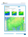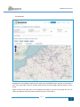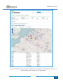
1
ATMOSYS User Manual Ref.: Deliverable 7/v03 23/04/2015 ATMOSYS User Manual Smeets Nele, Van Looy Stijn, Blyth Lisa VITO Partners: Lisa Blyth Email: [email protected] Tel: (+32-14) 33 67 57 27 95 http://www.vito.be http://www.life-atmosys.be Acknowledgements: http://www.lcsqa.org/ http://www.vmm.be http://www.irceline.be http://ec.europa.eu/environment/life ATMOSYS User Manual 1. 2. Introduction ________________________________________________________________ 5 Home ______________________________________________________________________ 6 Navigation through the Web Application _______________________________________________________________ 7 Interesting News __________________________________________________________________________________ 7 3. 4. 5. 6. Services ____________________________________________________________________ 8 Daily Forecast ______________________________________________________________ 10 4.1 Overview ________________________________________________________________________________ 10 4.2 Parameters ______________________________________________________________________________ 12 4.3 Changing the forecast date _________________________________________________________________ 12 4.4 Visualisation of the Air Quality Forecast Maps __________________________________________________ 13 4.4.1 Legend __________________________________________________________________________________ 14 4.4.3 Changing the Map in the Map Viewer _________________________________________________________ 14 4.5 Changing the Pollutant _____________________________________________________________________ 17 Forecast Validation __________________________________________________________ 18 5.1 Overview ________________________________________________________________________________ 19 5.2 Select Validation Period ____________________________________________________________________ 20 5.3 Select Pollutant ___________________________________________________________________________ 20 5.4 Selection of Measurement Station Types_______________________________________________________ 20 5.5 Selection of Station Observation Data _________________________________________________________ 21 5.5.1 The Measurement Stations Map Viewer _______________________________________________________ 23 5.5.2 Map Viewer Legend _______________________________________________________________________ 23 5.5.3 Measurement Station Table _________________________________________________________________ 23 5.6 Perform Validation ________________________________________________________________________ 24 5.7 Create Validation Charts ___________________________________________________________________ 26 5.7.1 Change Forecast Day ______________________________________________________________________ 28 5.7.2 Chart Functionality ________________________________________________________________________ 29 5.7.3 Chart type 1: Time Series ___________________________________________________________________ 29 5.7.4 Chart type 2: Scatter Plot ___________________________________________________________________ 30 5.7.5 Chart Values _____________________________________________________________________________ 31 5.8 Calculation of the Validation Statistics ________________________________________________________ 33 5.8.1 Export __________________________________________________________________________________ 35 Model Evaluation Tool _______________________________________________________ 36 6.1 Introduction _____________________________________________________________________________ 36 6.2 Upload model values and observations ________________________________________________________ 36 6.3 File format_______________________________________________________________________________ 38 6.4 Check the format of the uploaded files ________________________________________________________ 39 6.5 Remove uploaded file ______________________________________________________________________ 40 6.6 Remove all uploaded files ___________________________________________________________________ 41 Page 2 ATMOSYS User Manual 7. 8. 9. 6.7 Remove all model value files ________________________________________________________________ 41 6.8 Remove all observation files _________________________________________________________________ 41 6.9 Target plot tab ___________________________________________________________________________ 42 6.10 Parameters - Select & Validate Parameters ____________________________________________________ 42 6.11 Compute Target Plot_______________________________________________________________________ 43 6.12 Stations summary _________________________________________________________________________ 44 6.13 Time transformation_______________________________________________________________________ 44 6.14 Minimum data availability __________________________________________________________________ 44 6.15 Target plot ______________________________________________________________________________ 45 6.16 Summary statistics ________________________________________________________________________ 47 6.17 OBS Mean _______________________________________________________________________________ 48 6.18 OBS Exceed ______________________________________________________________________________ 49 6.19 TIME Bias Norm __________________________________________________________________________ 49 6.20 TIME Corr Norm __________________________________________________________________________ 49 6.21 TIME StdDev Norm ________________________________________________________________________ 49 6.22 TIME HPerc Norm _________________________________________________________________________ 50 6.23 SPACE Corr Norm _________________________________________________________________________ 50 6.24 SPACE StDev Norm ________________________________________________________________________ 50 6.25 Formulas ________________________________________________________________________________ 50 6.26 Configuration file ‘goals_criteria_oc.dat’ ______________________________________________________ 51 6.27 Export __________________________________________________________________________________ 51 6.28 Extra validation – Forecast Validation Tool Functionality __________________________________________ 55 6.29 Info ____________________________________________________________________________________ 58 Annual Air Quality Maps Archive _______________________________________________ 60 7.1 Overview ________________________________________________________________________________ 60 7.2 Load New Maps - Choose Pollutant & Indicator _________________________________________________ 62 7.3 Map Viewer - GIS Operations ________________________________________________________________ 64 7.4 Map Legend _____________________________________________________________________________ 64 Time Evolution Maps ________________________________________________________ 65 8.1 Overview ________________________________________________________________________________ 65 8.2 Loading New Maps ________________________________________________________________________ 67 8.3 Loading map data_________________________________________________________________________ 67 8.4 Viewing the Animation _____________________________________________________________________ 69 8.5 Share the Animation Video__________________________________________________________________ 71 Time Series ________________________________________________________________ 72 9.1 Overview ________________________________________________________________________________ 72 9.2 Choosing a Location _______________________________________________________________________ 73 9.3 Loading the time series_____________________________________________________________________ 74 Page 3 ATMOSYS User Manual 9.4 Analysis of the data _______________________________________________________________________ 75 9.5 Changing Viewing of the Pollutants ___________________________________________________________ 77 9.6 10. Export the data ___________________________________________________________________________ 77 Exposure tool ____________________________________________________________ 79 10.1 Overview ________________________________________________________________________________ 79 7.2 Selecting start and end time_________________________________________________________________ 80 7.3 Selecting a pollutant _______________________________________________________________________ 82 7.4 Selecting a statistic ________________________________________________________________________ 82 7.5 Output: population density _________________________________________________________________ 83 7.6 Output: calculated statistic _________________________________________________________________ 84 7.7 Output: histogram ________________________________________________________________________ 85 7.8 Output: cumulative distribution ______________________________________________________________ 87 7.9 Output: exposure summary _________________________________________________________________ 87 8 Help Service _______________________________________________________________ 89 9 Expertise __________________________________________________________________ 90 10 About __________________________________________________________________ 93 11 Contact details ___________________________________________________________ 94 12 References ______________________________________________________________ 96 Appendix 1: Statistics for model evaluation: DELTA tool ________________________________ 97 Appendix 2: Change log __________________________________________________________ 98 Page 4 ATMOSYS User Manual 1. Introduction The ATMOSYS web application is developed as part of the LIFE ATMOSYS project (http://www.lifeatmosys.be). The core goal of the ATMOSYS LIFE+ project is to demonstrate innovative solutions and knowledge, specifically designed to evaluate and analyse air pollution in European hotspot regions. This demonstrative system has being established for the European hotspot region of Flanders, north Belgium by VITO (Belgian scientific research institution) together with the Flemish Environment Agency (VMM). This system is a test environment for a multitude of state of the art air quality services. After a process of rigorous testing, some will become part of the official forecasts and assessments on ambient air quality in Belgium as published by Belgian Interregional Environment Agency IRCEL CELINE and Flanders as published by the Flemish Environment Agency VMM. The demonstrative website allows potential users to explore the various services and information available in a real test case environment. There are 6 main parts to the website: • • • • • • Home News Services Expertise About Contact Each of them will be described in a separate chapter. A chapter will also be dedicated to each of the services. The ATMOSYS web application is available at the following URL:http://atmosys.eu/ Page 5 ATMOSYS User Manual 2. Home When opening the web application in a browser, the home page of the application is shown (see Figure 1). This home page contains some general information about the web application. Figure 1: Home page Page 6 ATMOSYS User Manual Navigation through the Web Application From this page, the various services and information can be accessed. The web application is spilt into 5 main parts. 1. 2. 3. 4. 5. News Services Expertise About Contact The simplest way to access each part is by using the banner above: However you can also click on one of the main headings in the first half of the page to reach respectively the Services, Expertise and About pages: Finally you can also take a short cut to one of the services by clicking on one of the individual services in the list at the bottom of the page. Interesting News In the second half of the page, the most recent interesting items relating to the project and/or application are shown. At the time of writing the ATMOSYS film is available to view and download alongside a glimpse of the latest news items. Page 7 ATMOSYS User Manual 3. Services Here a short overview of each of the seven services is given. The services are split into two main categories: Forecast and Assessment Services as shown by the selection pane on the left. Figure 2: Services Page Page 8 ATMOSYS User Manual Under the Forecast Services, there are two main services: 1. Demonstration of an harmonized AQ Forecast Service for Belgium 2. Interactive Forecast validation tool that can be used to ‘validate’ the demonstration forecast The Assessment Service section offers five different demonstrative tools for exploration: 1. Archive of annual concentration maps of AQ pollutants for Belgium 2. Time evolution maps of the above 3. Time series tool to extract a time series for a particular pollutant for a specific location from the maps above. 4. Model evaluation tool to evaluate AQ models based on the FAIRMODE Delta tool 5. Exposure calculation tool to calculate "human exposure" to a chosen pollutant, based on the chosen simulation results and given population data (in inhabitants per km²) for region. These tools offer the capability to access, visualize and analyse an archive of historic air quality maps for a specific region/country. The user friendly interface also allows the user to extract the complete set of hourly maps to obtain a better insight into specific pollution episodes. To access these individual service demonstrations, click on the Service header or the More info tab at the end of each service description. Figure 3: Navigation from the Services Page The final service shown is the Help Service. Here you will find this user manual, some information on the Delta benchmarking tool and examples files for the ATMOSYS model evaluation tool. Page 9 ATMOSYS User Manual 4. Daily Forecast 4.1 Overview Under the air quality forecast service tab, a demonstration of a 3 day forecast for Particulate Matter (PM10, PM2.5), Elementary Carbon (EC), Nitrogen Dioxide (NO2) and Ozone (O3) is provided. The maps shown here at the launch of the system are taken from a test service established for the Belgian Interregional Cell for the Environment. By default, the NO2 daily maximum map for the most recent forecast day available (normally today) is shown in the main viewer, as shown in Figure 2. Above the main viewer, the maps for the three consecutive forecast days (day +0, day + 1 and day + 2) are shown. Page 10 ATMOSYS User Manual Figure 4: Visualization of the forecast service for Belgium (forecast day 0) Page 11 ATMOSYS User Manual 4.2 Parameters At the top part of the page the current selected forecast date, the period for which data is available, the chosen pollutant, the indicator and the unit are shown. 4.3 Changing the forecast date By clicking on the current date, or on the icon to the right of it, a calendar component is shown: Page 12 ATMOSYS User Manual Another date can be selected by clicking on one of the available days. Days outside the available period are disabled and cannot be chosen. The arrows (<, >) at the top can be used to navigate to the previous or next month. The double arrows (<<, >>) can be used to go to the previous or next year. When a new date is chosen (e.g. 02-10-2013), you must click on the ‘Load’ button to load the corresponding maps. The currently selected date is then shown in the title of the map shown in the main viewer: Figure 5: Selection of another date 4.4 Visualisation of the Air Quality Forecast Maps Each day, the service provider computes forecasts for three consecutive days, starting from the current day. E.g. on October 3, forecasts are computed for October 3 (day 0), October 4 (day 1), and October 5 (day 2). At the top of the page, the three images are shown that correspond to the three forecast days. Each image shows the model output for the complete region covered by the selected service. These three images can be used by the user to compare the different forecasts in a quick way. Under these images, the forecast (day+0) for the current day is presented in the main viewer. The pollutant, indicator, unit, selected date and selected forecast day are shown in the map title (the blue header above the map). The viewer offers standard GIS functionalities such as zooming and panning. The scale of the map is shown in the bottom left-hand corner. The transparency of the concentration map can be changed by using the slider above. Page 13 ATMOSYS User Manual 4.4.1 Legend The legend of the maps is shown at the right of the viewer (Figure 6). Figure 6: The map legend The legend shows the meaning of the colors that are used in the maps. The units are shown above by the pollutant. 4.4.2 Main Map Viewer - GIS Operations The geographical data is visualized in a GIS viewer that allows the user to perform typical GIS operations: • • • • Zooming: Zooming is done by selecting the map, and then using the mouse wheel to zoom in or out. An alternative method is to use the slider at the left of the map window. By clicking on the plus or minus sign, or by dragging the slider up or down, you can zoom in or out. Panning: Panning can be done by clicking and dragging. Scale: The scale of the map is shown in the bottom left corner. Transparency: The transparency of the concentration map can be changed by using the slider in the header bar above the map viewer. Figure 7: The transparency slider 4.4.3 Changing the Map in the Map Viewer By default, forecast day 0 for the pollutant NO2 (daily max concentration) is selected in this map viewer. When the user wants to study one of the three forecast days in more detail, he clicks on one of the three images. The corresponding map is then shown in the map viewer below. Page 14 ATMOSYS User Manual Figure 8 and Figure 9 show forecast day 1 and forecast day 2 respectively. The selected forecast day is surrounded by a dotted border, and the title above is shown in a larger font. Figure 8: Visualization of forecast day 1 in the main viewer (4 October) Page 15 ATMOSYS User Manual Figure 9 : Visualization of forecast day 2 (5 October) Page 16 ATMOSYS User Manual 4.5 Changing the Pollutant By default, the NO2 daily maximum map for the most recent forecast day available (normally today) is shown in the main viewer. To visualize another pollutant concentration map, click on the pollutant drop down menu box to view the other pollutants available. For ozone it is possible to view the 1h maximum or the 8h maximum concentration maps. When you have chosen the new pollutant, click on the load button to upload the corresponding maps. The legend shown in the main viewer will change depending on the pollutant being shown. Page 17 ATMOSYS User Manual 5. Forecast Validation The validation tab allows a user to validate the model output of a chosen ATMOSYS air quality forecast using measurement data. It is developed to allow a user to validate recent model forecasting results (ideally over a few days), automatically on the fly. The tool uses the same basic validation statistics as those developed by JRC under the FAIRMODE SG4 working group model benchmarking initiative which led to development of the Delta tool. In consultation with JRC, an on-line version of the desktop Delta tool has also been developed (chapter 6) within ATMOSYS. The on-line model evaluation tool, in contrast to this ‘quick-check’ validation page is initially aimed at users who wish to evaluate long term retrospective simulations. Validation is done using (non-validated) observations of IRCEL-CELINE that are published using a SOS service. Page 18 ATMOSYS User Manual 5.1 Overview Figure 10 :Forecast validation page. By default the end validation day is the last week of the available period is selected. The end date is thus most often today’s date (3rd October 2013) and the start date (28th September 2013) is 7 days earlier. Figure 10 shows the main parts of the validation web page. At the top of the page the user can select the validation period and the parameters that he is interested in. Page 19 ATMOSYS User Manual In the main window, there are four tabs containing a map (stations tab), charts, validation statistics and export functionality for the model output corresponding to the selected parameters. At the top of the Stations tab, the user can select the day that he wants to validate, by selecting one of the radio buttons: Forecast day+0, Forecast day+1, Forecast day+2. The map underneath shows all measurement stations that are in the service’s region and for which the service provider has computed time series. In the Charts tab, two charts are included. The first chart shows one or more time series of model data and observations. The second chart is a scatter plot. In the Statistics tab, some statistics are shown. The Export tab allows the user to export the validation results. 5.2 Select Validation Period The period that is validated can be changed by changing the start date and end date at the top of the page (see Figure 11). By default, the last week of the available period is selected. Dates can be changed using the drop down calendar as described in section 4.3. Figure 11: Change the validation period 5.3 Select Pollutant The pollutant is selected using the pollutant drop down menu box. 5.4 Selection of Measurement Station Types There are four classes of station types given as demonstrated in Figure 12. The user can select all of the station types or they can select only one of the classes. Page 20 ATMOSYS User Manual Figure 12: Change the validation period 5.5 Selection of Station Observation Data After all the selections click on the button so that all the available measurement stations (or for that chosen class) for the chosen pollutant, the specific forecast day (day+0, +1, +2) and time period will be made available for the validation step. In this step a query of the SOS (Sensor Observation Service) service at the Belgian Interregional Agency is undertaken. A SOS service is a web service interface which allows querying observations, sensor metadata, as well as representations of observed features. In the SOS, for each of these measurement stations, hourly concentration values are available, for all days in the available period, and for each of the three forecast days. This enables the user to carry out validations for each of the forecast days, and for each of the days in the available period. Figure 13: Retrieving the data from the SOS Once this query is complete the the show stations button. message appears in place of In addition, the available stations are now visible both in the map viewer (see Figure 13) and in the table underneath. Page 21 ATMOSYS User Manual Figure 14 Validation Page showing all the NO2 measurement stations available for the Forecast +0 day for the period 15th August until 31st August 2013 Page 22 ATMOSYS User Manual 5.5.1 The Measurement Stations Map Viewer The map shows the available measurement stations and modeled time series output for the chosen pollutant, the specific forecast day (day+0, +1, +2) and time period (see Figure 14 above). The geographical data is visualized in a GIS viewer that allows the user to perform typical GIS operations as explained in section 4.4.2. 5.5.2 Map Viewer Legend There are different types of stations. Each type has a different color: purple (industrial), orange (background), blue (traffic), and green (unknown). These colors correspond to the colors that are used on the European Air quality database website EIONET - AirBase. The corresponding legend is shown on the top right hand corner of the map, as shown in Figure 15. Figure 15: The legend for the measurement stations 5.5.3 Measurement Station Table The table underneath this map shows the same list of stations. This table shows the station ID, the station name and the station type. Use the scroll bar on the right to view the rest of the stations. Figure 16: The measurement stations selected The 3 headings categories can also be filtered in ascending or descending order. Page 23 ATMOSYS User Manual 5.6 Perform Validation The next step is to choose the measurement stations that you wish to use for the validation. This can be done in two ways: 1 Click on a measurement station in the map. The size of the triangle increases to indicate that the station is selected. When you want to select more than one measurement station, then use the CTRL button when clicking on the additional stations. The stations are automatically selected in the table underneath the map; selected stations in the table are indicated in blue. 2 Click on a measurement station in the table. The selected row is indicated in blue. When you want to select more than one station, then use the CTRL button when clicking on the additional stations. The stations are automatically selected in the map. It is also possible to select a range of stations by clicking on one item, and then shift-clicking on another stations; all stations in between will be selected. For example, in Figure 17, four stations are selected: BETR020, BETR841, BETM702 and BETN121. Page 24 ATMOSYS User Manual Figure 17: Four stations are selected on the map and in the table: BETM702 (Ertevelde Industry),BETN121 (Offagne – Background), BETR020 (Vilvoorde - Traffic) and BETR841 (Mechelen Background) Page 25 ATMOSYS User Manual Once the stations are chosen and you are ready to validate, click the button! 5.7 Create Validation Charts Once the validation occurs, the charts window will automatically open showing two charts that have been computed. These charts are as shown in Figure 18. The top one is a time series chart showing the measurement and modeled concentration values for the chosen pollutant over the chosen period. The other is a scatter plot for the modeled values vs. the observation values. Further detail is given below in section 5.7.4. Page 26 ATMOSYS User Manual Figure 18: The Validation charts: for the period 15th August until 31st August 2013 Page 27 ATMOSYS User Manual 5.7.1 Change Forecast Day By default, the first forecast day (Forecast day 0) is selected. When the user wants to validate another forecast day, he selects one of the radio buttons at the top of the Stations tab (see Figure 19) . Figure 19: Selection of the forecast day When clicking the “Validate” button after this, the charts and statistics will use the selected forecast day. The forecast day that is used in the computations is shown in the map: and chart titles: Page 28 ATMOSYS User Manual 5.7.2 Chart Functionality Both charts have the following functionalities: • For all selected stations, the corresponding observations and model values are added to the time series chart and the scatter plot. • The period shown in the charts corresponds to the period that is selected in the upper left corner of the page. • The same color is used in both charts for the same station. • The legends of the charts contain the name of the station and make clear whether the corresponding data represent observations or model output. • By right-clicking on a chart and selecting “Save Picture As” (or “Save Image As”, depending on the browser), the user can save the chart as PNG and use it in its own reports. In the following paragraphs, the two chart types are discussed in more detail. 5.7.3 Chart type 1: Time Series Figure 20: Time series chart example An example of a time series chart is shown in 15th August until 31st August 2013 Figure 20. Page 29 ATMOSYS User Manual • • • • • This chart contains both observations (points), and model output (lines) for the selected station(s). Observations and model output that correspond to the same station have the same color. The X-axis shows the time; the Y-axis shows the concentration (in µg/m³). The model results are connected by a spline. The period that is shown corresponds to the validation period that was selected by the user. The title of the chart shows the name of the service, the forecast day, the pollutant and the validation period. 5.7.4 Chart type 2: Scatter Plot Figure 21: Scatter plot example An example of a scatter plot is shown in Figure 21. For more information about this type of chart: http://en.wikipedia.org/wiki/Scatter_plot. • • • • This chart contains both observations and model output for the selected station(s). Each point represents a model concentration and the corresponding observation (for the same timestamp). The value of the model concentration is shown on the Y-axis; the value of the observation is shown on the X-axis. The chart shows data for the selected validation period. The identity line (y= x) is drawn as a reference. Two other lines (y = 2x and y = 0.5x) are also shown. For each station, a line of best fit (or trend-line) is shown in the same color as the model/observation values. Page 30 ATMOSYS User Manual • • The correlation coefficient (R²) is also shown in the chart and in the legend. The title of the chart shows the name of the service, the forecast day, the pollutant and the validation period. 5.7.5 Chart Values At the end of page there is the option to change the averaging period. By default the hourly values are for the selected period are shown. However if you wish to validate the daily average, daily maximum values etc., this is done using the drop down menu as show in Figure 22 Figure 22 Drop down menu of the different averaging periods avialable When you press the button the charts for that new averaging are computed. In Figure 22 the daily average values are given for the chosen period above are given. Page 31 ATMOSYS User Manual Figure 23: New Validation Charts for the daily Averge Page 32 ATMOSYS User Manual The following possibilities are available: • • • • • • • daily average daily maximum daily maximum of the eight-hour averages monthly average (when the selected period is longer than one month) average day and night concentration 24 values, where the i-th value is the average of all observations/model values corresponding to the i-th hour of the day, for all days in the selected period. E.g. when the selected period consists of 8 days, then the i-th value is the average of 8 values, each corresponding to the i-th hour of the day. 7 values, where the i-th value is the average of all observations/model values corresponding to the i-th day of the week (where Monday is the first day of the week, Tuesday is the second day, …) for all days in the selected period. This is only meaningful when the selected period is longer than one week. By selecting a new value in the drop-down list, and by clicking the “Compute” button, the charts will be updated to show the selected option. 5.8 Calculation of the Validation Statistics Under the statistics tab, a list of available statistic calculations is given. This list is based on the core statistics available within the DELTA tool. Appendix 1 gives an overview of these statistics . The user is able to dynamically choose the statistics that he wants to use. A list of all available statistics is shown in the first left hand frame. From this list, the user can choose the ones that he is interested in. This can be done by doubleclicking on the statistic, or by selecting the statistic and then clicking on the “Copy” button. Multiple statistics can be selected by using CTRL-click or SHIFT-click. All statistics can be copied at once by using the “Copy all” button. Copied statistics will appear in the list at the right. Copied statistics can be deselected (i.e. moved to the list at the left) in a similar way by using the “Remove” buttons, or by double-clicking in the list at the right. Page 33 ATMOSYS User Manual When clicking on the “Compute” button, a table is shown containing the selected statistics (columns), with values for each selected station (rows). Two of the statistics (Relative Directive Error and Relative Percentile Error) make use of a limit value and the maximum number of exceedances of a certain limit value. Since these values change in time, and since different organizations are interested in different limit values, these values are specified as input values. This information is available in the web application by clicking on the question mark ( ). Figure 24: The validation statistics tab Page 34 ATMOSYS User Manual 5.8.1 Export The validation results can be downloaded in the Export tab. The results consist of: The selected parameters: o service name o start date o end date o pollutant o forecast day (0, 1 or 2) o stations The observations and model values for the selected stations. In both cases, the timestamp and corresponding value are given. The data used for the scatter plot, for each selected station. The observations are in the first column, the corresponding model values are in the second column. The values of the different statistics, computed for each station. Figure 25: The Export tab. Two versions of the CSV file are made available. The first CSV file uses the Dutch settings, which uses the semi-colon (;) as delimiter and the comma (,) as decimal separator. When the regional settings of the user’s machine are in Dutch, this file can be automatically opened in Excel. The second CSV file uses the English settings, which uses the comma (,) as delimiter and the period (.) as decimal separator. Page 35 ATMOSYS User Manual 6. Model Evaluation Tool 6.1 Introduction The ATMOSYS model evaluation tool is based on the desktop Delta tool (http://aqm.jrc.ec.europa.eu/DELTA/index.htm) that is being developed by JRC in the context of the FAIRMODE working group on air quality assessment http://fairmode.jrc.ec.europa.eu/wg1.html. The target plot and the summary statistics table developed for the Delta tool for one year of hourly values are included in the ATMOSYS online tool. The current ATMOSYS implementation corresponds to version 5.1 of the Delta tool ([1]). At this moment the tool is configured for the pollutants NO2, O3, PM10 and PM2.5 but by changing a configuration file (‘goals_criteria_oc.dat ‘) which is the same as for the JRC DELTA tool other pollutants can be included. The online model evaluation tool is composed of six main tabs: • • • • • • Upload Target plot Summary statistics Export Extra validation Info The different functionalities will be discussed in the following sections. 6.2 Upload model values and observations The Upload tab (see figure 26) allows the user to upload files containing model values (at the left) and observations (at the right). The format of these files is explained in section 6.3. Each file contains data for one station. The file name should reflect the station name. Model value files and observation files are matched based on their file name, so files containing data for the same station should have the same name. Figure 26: The upload tab Page 36 ATMOSYS User Manual When clicking on the Upload file… button, a file dialog (Figure 27) is opened, which allows the user to select one or more CSV files on its local file system. Figure 27: When clicking on ‘File upload…’, a file dialog is opened After selecting the files (Figure 28), the Open button should be clicked. The selected files will then be uploaded to the server. Figure 28: The user selects one or more CSV files The selected files are listed in the Upload tab, as shown in Figure 29. Page 37 ATMOSYS User Manual Figure 29: The names of the uploaded files are listed alphabetically 6.3 File format The model values and observations should be included in CSV files in which individual fields are separated by semi colons. Each file contains hourly values for one year, for one station and for one or more pollutants. The name of the CSV file is equal to the name of the station, followed by the extension ‘.csv’. The model values and observations are included in different files. The first line of the file should be a header: year;month;day;hour;pollutant (for one pollutant) or year;month;day;hour;pollutant1;pollutant2;… (for multiple pollutants) where pollutantX corresponds to one of the pollutant names in the configuration file and should with the current version of the configuration file be one of NO2, O3, PM10, PM25. Page 38 ATMOSYS User Manual The other lines are (in the case of one pollutant) have the structure: 2007;01;01;00;123.2 2007;01;01;01;243.7 ... 2007;12;31;23;25.8 where the fields separated by semi colons from left to right are: • • • • year: 4 digits month: 1-12 day: 1-31 hour: 0-23 Leap years are not taken into account, so a file always contains 8760=365*24 values. Some other rules: • • • • If data are missing the gaps should be filled by -999 Each blank row or rows beginning with "[", ";" or "#" will be discarded No spaces are permitted between the fields Decimal separator is '.' An example CSV file can be downloaded from the Help tab (see section 8). 6.4 Check the format of the uploaded files The format of the uploaded files can be checked by clicking the Check format button. Depending on the number of files to check, checking the uploaded files can take up to several minutes. During upload the hour glass appears. When all files are checked and valid, then a green message is shown above the upload component indicating that the validation is ok. Page 39 ATMOSYS User Manual When the format of one of the files is invalid, then an error message is shown above the upload component. The message is shown in red, and contains the name of the file, the line number, and a description of the error. 6.5 Remove uploaded file An uploaded file can be removed by clicking the Remove button to the right of the file. Page 40 ATMOSYS User Manual 6.6 Remove all uploaded files By clicking the Remove all button, all uploaded model values files and observations files are removed at once. 6.7 Remove all model value files By clicking the Remove model value files button, all uploaded model value files are removed. 6.8 Remove all observation files By clicking the Remove observation files button, all uploaded observation files are removed. Page 41 ATMOSYS User Manual 6.9 Target plot tab The Target plot tab allows the user to compute a target plot for the uploaded observations and model values. There are three panels: • • • Parameters Stations summary Target plot The three panels will be discussed in the following sections. Figure 30: The target plot tab 6.10 Parameters - Select & Validate Parameters To verify what data is available relative to the loaded files, the user must first click Read file Parameters. The total period and the pollutants available will then appear in the parameters window (Figure 31). Page 42 ATMOSYS User Manual The user can alter the validation period by selecting a start and end date. Changing a date is explained in section 4.3. The pollutants available will be shown as options in the pollutant drop-down menu. Underneath the pollutant name shown in the pollutant drop-down menu the values for the different parameters used in the measurement uncertainty calculation are listed that correspond to that pollutant name: alpha, U, RV as well as the limit values for the number of exceedances and the data availability criterion. These parameter values are read from the ‘goals_criteria_oc.dat’ configuration file which is also used by the JRC DELTA application. Figure 31: Target plot tab screen after parameters have been computed 6.11 Compute Target Plot The computation of the target plot can be started by clicking the Compute Target Plot button. This button is disabled until the user clicks the Read file Parameters button. After clicking the button, all uploaded model value and observations files are read, and the selected validation period is extracted. In the selected validation period, at least 75% of the modelobservation tuples for a given station should be effective; otherwise, the station is ignored. When a model value file and observation file have the same name, then they are associated with each other. When a model file has no corresponding observation file, then this file is ignored (and the other way round). When all files are read, the target plot and summary statistics are computed for the stations for which both a model value and observation file is available, and that contain more effective tuples Page 43 ATMOSYS User Manual in the selected validation period than required by the data availability criterion which is currently set at 75% . This can take some time... 6.12 Stations summary The stations summary panel contains an overview of the uploaded files (Figure 32). There are three categories: • • • OK: Stations for which both a model value and observation file are uploaded. For the selected period, more than 75% of the model–observation tuples are effective. Missing file: Stations for which the model value file or observation file is missing. Insufficient tuples: Stations for which both a model value and observation file are uploaded. For the selected period, less than 75% of the model–observation tuples are effective. Figure 32: Stations summary 6.13 Time transformation Before computing the target plot and the summary statistics, the following transformations are computed which are determined from the settings in the configuration file ‘goals_criteria_oc.dat’ and which are currently set as follows: Pollutant NO2 O3 PM10 6.14 Transformation Moving 3-hour average, using the values at hours -2, -1, 0. Hourly values (‘raw data’) Daily maximum of eight hour moving average, using the values at hours -7, -6, -5, -4, -3, -2, -1, 0 Daily average Minimum data availability As described above, at least 75% of the tuples in the selected validation period should be effective. Otherwise, the target plot and summary statistics cannot be computed for a station. Page 44 ATMOSYS User Manual This 75% limit is also applied when computing the time transformations. E.g. when computing a daily average, at least 18 of the 24 hourly values should be effective. If not, the daily average cannot be computed for that day. When computing an eight hour moving average, at least 6 of the 8 hourly values should be effective, otherwise the moving 8 hour average for that hour cannot be computed. 6.15 Target plot The target plot (Figure 33) shows two statistics for each station. Each station is represented by its own color and/or shape in the plot, which is shown in the legend below the target plot. The x-value is given by: 𝐶𝑅𝑀𝑆𝐸 2 ∗ 𝑅𝑀𝑆𝑈 where 𝑁 1 ̅ ) − (𝑂𝑖 − 𝑂̅)]2 𝐶𝑅𝑀𝑆𝐸 = √ ∑[(𝑀𝑖 − 𝑀 𝑁 𝑖=1 The value of CRMSE is always positive. The following sign function determines whether the x value is positive or negative. When |𝜎𝑂 − 𝜎𝑀 | √2𝜎𝑂 𝜎𝑀 (1 − 𝑅) ≥1 then the sign is 1. Otherwise, the sign is -1. The formula for the Pearson correlation coefficient R, for the standard deviations and for RMSU can be found in section 6.25. The y-value is given by: 𝑀𝐵𝑖𝑎𝑠 2 ∗ 𝑅𝑀𝑆𝑈 where 𝑁 1 𝑀𝐵𝑖𝑎𝑠 = ∑(𝑀𝑖 − 𝑂𝑖 ) 𝑁 𝑖=1 Page 45 ATMOSYS User Manual The target plot shows two circles: • • the solid circle has radius 1. the dashed circle has radius 0.5. The percentage of the stations that is inside the solid circle and that represent stations that fulfil the model quality objective criterion is shown in the upper left corner of the target plot. In the upper right corner are the values of the parameters that are used for calculating the observation uncertainty that are read from the configuration file. In addition the chosen period, time aggregation (in this case hourly) and pollutant name are given in the subtitle. Figure 33: Target plot Page 46 ATMOSYS User Manual 6.16 Summary statistics In the summary statistics tab (Figure 34), different statistics are computed for the stations. The first column shows three different categories: • • • OBS: Statistics for the given observations. TIME: Statistics computed for each of the stations using the given (time-transformed) values (see section 6.13). SPACE: Statistics computed for the whole model domain using average values per station. The second column contains six different statistics, which are described in the following sections. In the case of the TIME statistics the third column contains a green circle when more than 90% of the blue dots are inside the green or orange range in the fourth column. For the SPACE statistics there is only a single dot and the circle will therefore only be green if this single dot is inside the green or orange range in the fourth column. The fourth column shows the calculated statistics. For the categories OBS and TIME a statistic is computed for each station and each blue dot corresponds to a single station. For the category SPACE, only one spatial statistic is computed, so there is only one blue dot. The blue dots for stations for which the model performance criterion is fulfilled lie within either the green or the orange shaded areas. If a dot falls within the orange shaded area the error associated with the particular statistical indicator is dominant albeit still small enough for compliance. Page 47 ATMOSYS User Manual Figure 34: Summary statistics table 6.17 OBS Mean For each station, the mean observation is computed: 𝑁 1 𝑂̅ = ∑ 𝑂𝑖 𝑁 𝑖=1 The resulting means for each of the stations are presented as blue circles. Page 48 ATMOSYS User Manual 6.18 OBS Exceed For each station, the number of exceedances of a limit value is computed. The limit value is dependent on the selected pollutant and is read from the configuration file. It is shown in the second column. 6.19 TIME Bias Norm For each station, the normalized mean bias (NMB) is computed in the following way: 𝑁𝑀𝐵 = ̅ − 𝑂̅ 𝑀 ̅̅̅̅̅̅̅̅̅̅̅̅̅ 2 ∗ 𝑅𝑀𝑆𝑈 The limit values for the normalized mean bias are: −1 ≤ 𝑁𝑀𝐵 ≤ 1 6.20 TIME Corr Norm For each station, the normalized correlation is computed in the following way: 𝐶𝑜𝑟𝑟𝑁𝑜𝑟𝑚 = (1 − 𝑅) 𝜎𝑜 2 2 𝑅𝑀𝑆𝑈 2 The limit values for the normalized correlation are: 0 ≤ 𝐶𝑜𝑟𝑟𝑁𝑜𝑟𝑚 ≤ 1 6.21 TIME StdDev Norm For each station, the normalized standard deviation is computed in the following way: 𝑆𝑡𝐷𝑒𝑣𝑁𝑜𝑟𝑚 = 𝜎𝑀 − 𝜎𝑂 2 ∗ 𝑅𝑀𝑆𝑈 The limit values for the normalized standard deviation are -1 and 1: −1 ≤ 𝑆𝑡𝐷𝑒𝑣𝑁𝑜𝑟𝑚 ≤ 1 Page 49 ATMOSYS User Manual 6.22 TIME HPerc Norm To provide insight on the model capability to reproduce extreme events (e.g. exceedances) a model performance criterion for percentiles was introduced, HPercNorm: 𝑀𝑝𝑒𝑟𝑐 − 𝑂𝑝𝑒𝑟𝑐 2𝑈(𝑂𝑝𝑒𝑟𝑐 ) in which Mperc and Operc are respectively the observed and modeled value corresponding to a certain percentile and U(Operc) is the observation uncertainty corresponding to the observed value for a specific percentile. For pollutants and time aggregation values for which limit values for number of exceedances have been set by legislation these limit values can be used to determine appropriate percentiles. In other cases the 95th percentile is used. HPercNom = 6.23 SPACE Corr Norm First, the average observation and average model value is computed for each station. Using these average values, the normalized correlation is computed, as described in section 6.20. The result of the computation is only one value, so only one blue dot is shown. 6.24 SPACE StDev Norm First, the average observation and average model value is computed for each station. Using these average values, the normalized standard deviation is computed, as described in section 6.21. The result of the computation is only one value, so only one blue dot is shown. 6.25 Formulas 𝑁 ̅= 𝑀 1 ∑ 𝑀𝑖 𝑁 𝑖=1 𝑁 1 𝜎𝑂 = √ ∑(𝑂𝑖 − 𝑂̅)2 𝑁 𝑖=1 𝑁 1 ̅ )2 𝜎𝑀 = √ ∑(𝑀𝑖 − 𝑀 𝑁 𝑖=1 𝑁 𝑁 𝑁 ̅ )(𝑂𝑖 − 𝑂̅)⁄√∑(𝑀𝑖 − 𝑀 ̅ )2 √∑(𝑂𝑖 − 𝑂̅)2 𝑅 = ∑(𝑀𝑖 − 𝑀 𝑖=1 𝑖=1 Page 50 𝑖=1 ATMOSYS User Manual 𝑅𝑀𝑆𝑈 = 𝑘𝑈𝑟𝑅𝑉 √(1 − 𝛼)(𝑂̅2 + 𝜎𝑜2 ) + 𝛼. 𝑅𝑉 2 The parameters (𝑘, 𝑢𝑟𝑅𝑉 , α, 𝑅𝑉) are read from the configuration file ‘goals_criteria_oc.dat’. 6.26 Configuration file ‘goals_criteria_oc.dat’ The computation of the different statistics uses different values that are different for each pollutant. These values are read from the configuration file ‘goals_criteria_oc.dat’. This file is also used by the JRC Delta tool. As the development of the benchmarking procedure within the FAIRMODE community is an ongoing activity the current values in this configuration file could still change. It was therefore decided to also base the ATMOSYS benchmarking tool on this same configuration file to ensure that changes to the parameters in the JRC Delta tool can easily be adopted in ATMOSYS. A description of this file can be found in the Delta tool manual [1]. The current values in the file can be found in the table below. 6.27 Pollutant Time aggregation NO2 PM10 PM25 O3 hourly value daily average daily average daily maximum average Limit value k*𝑢𝑟𝑅𝑉 (µg/m³) (%) 200 50 25 8-hour 120 24 28 36 12.6 α 0.04 0.018 0.035 0.62 Export The export tab (Figure 35) allows the user to download a PDF file or CSV (comma-separated values) file that contains the results of the model evaluation tool, including the target plot, and the summary statistics. Page 51 ATMOSYS User Manual Figure 35: Export tab When clicking on the PDF download link, a dialog is opened, which allows the user to save the PDF file, or to open it using an appropriate program. Figure 36, Figure 37 and Figure 38 show an example of such a PDF file. It contains an overview of the selected parameters, the stations summary, target plot and the summary statistics table. Figure 36: Exported PDF file: page 1 Page 52 ATMOSYS User Manual Figure 37: Exported PDF file: page 2 Page 53 ATMOSYS User Manual Figure 38: Exported Pdf file: Page 3 Page 54 ATMOSYS User Manual A CSV file is also available for download. This contains an overview of the selected parameters, the stations summary, the values of each station in the target plot and values of the summary statistics table, including the range values. The (time-transformed) tuples that are used in the target plot and summary statistics are listed at the end of the CSV file. The values are listed per station. This file can be downloaded by clicking on the URL labeled ‘Download report as CSV’ Finally, the summary statistics can be downloaded as a single PNG by clicking the last URL. 6.28 Extra validation – Forecast Validation Tool Functionality The Extra validation tab (Figure 39) allows the user to use the forecast validation tool (as described in section 5) functionalities to further analyse the uploaded observations and model values. Thus Page 55 ATMOSYS User Manual to generate scatter plot and time series charts and run other statistics. The statistics will be computed on the time-transformed tuples described in section 6.13. This tab only becomes available once the previous tabs -Upload, Target Plot, and Statistics- have been used i.e. only after uploading one or more files in the Upload step (section 6.2), checking the format of these files, and computing the target plot the Extra validation tab will be enabled. By default, the last week of the selected period is selected for the pollutant that is selected in the target plot tab. The user can select a start and end date and then click the Start validation button. When clicking this button, the charts and statistics are computed and shown in the Charts and Statistics tabs underneath. These charts and statistics correspond to those computed in section 5. Figure 39: Extra validation tab Page 56 ATMOSYS User Manual Page 57 ATMOSYS User Manual Figure 40: Extra Validation tab after the validation Figure 41: Statistics tab, containing uploaded data 6.29 Info The Info tab (Figure 42) contains information about the functionality and use of the model evaluation tool. Page 58 ATMOSYS User Manual Figure 42: Info tab Page 59 ATMOSYS User Manual 7. Annual Air Quality Maps Archive 7.1 Overview The annual air quality maps service is an archive of annual average concentration maps of Particulate Matter (PM10, PM2.5), Elementary Carbon (EC), Nitrogen Dioxide (NO2) and Ozone (O3). This demonstration system is established for the Belgian Inter-regional environmental agency and contains at the time of writing only maps for the year 2009. The system is established so that future maps can be easily made and uploaded based on the 2009 set-up. These high resolution maps are generated using RIO, an interpolation model, coupled with IFDM, a bi-gaussian plume model. The exception is the map for the pollutant EC, which was computed using AURORA, a chemical transport model, coupled with IFDM. In line with the air quality legislation, several specific statistical indicator maps for each pollutant, like the number of exceedences of the daily threshold allowed for PM10 are provided. Page 60 ATMOSYS User Manual Figure 43: Annual Air Quality Maps Page Page 61 ATMOSYS User Manual 7.2 Load New Maps - Choose Pollutant & Indicator By default, the EC annual average concentration map for 2009 is shown in the main viewer. As for the previous services the pollutant can be changed via the pollutant drop-down list (Figure 45). Figure 44: Annual Air Quality Maps Page – Pollutant Options Likewise the required specific statistical indicator can be chosen via the indicator drop-down menu (see Figure 45). To load the new map in the main viewer, click LOAD. Under each indicator an explanation is provided. For example, AOT60ppb-max8u is ‘the cumulative sum of the daily maximum 8 hour average concentration exceeding 60 ppb’. Page 62 ATMOSYS User Manual Figure 45: Annual Air Quality Maps Page showing (above) the drop down indicators available for NO2 and (below) the resulting NO2 map after choosing to visualize the map showing the number of exceedences of the European limit value of 200 µg/m3 Page 63 ATMOSYS User Manual 7.3 Map Viewer - GIS Operations The maps are visualized in a GIS viewer that allows the user to perform typical GIS operations: • • • • Zooming: Zooming is done by selecting the map, and then using the mouse wheel to zoom in or out. An alternative method is to use the slider at the left of the map window. By clicking on the plus or minus sign, or by dragging the slider up or down, you can zoom in or out. Panning: Panning can be done by clicking and dragging. Scale: The scale of the map is shown in the bottom left corner. Transparency: The transparency of the concentration map can be changed by using the slider in the header bar above the map viewer. Figure 46: The transparency slider 7.4 Map Legend The legend of each map is shown at the right of the viewer (Figure 6). The unit can be found within the map title, together with the pollutant: Figure 47: The map legend The legend shows the meaning of the colors that are used in the maps. Page 64 ATMOSYS User Manual 8. Time Evolution Maps 8.1 Overview One of the user requirements during the latter iterations of the system was to provide a functionality that would allow visualization of specific episodes. Instead of loading specific episodes it was decided to provide this functionality for the annual maps that are already loaded into the archive. These annual maps are essentially made up of 8760 hourly maps which were generated using RIO, an interpolation model, coupled with IFDM, a bi-gaussian plume model. Again for EC, the maps were produced using AURORA, a chemical transport model, coupled with IFDM. For the time evolution visualization, 24h moving average maps are calculated from the hourly map database for the selected period. The 24h period over which the average is made starts at the selected hour and ends 23 hours later. For maximum performance, the period chosen is restricted to two weeks, a maximum of 335 hours; from 00:00 day 1 to 23:00 on day 14. With a user-friendly interface, the user is able to scroll through these maps to get an ‘hourly’ view of a specific air pollution episode that occurred during a period. Page 65 ATMOSYS User Manual Figure 48: The Time Evolution maps page Page 66 ATMOSYS User Manual 8.2 Loading New Maps By default, the EC annual average concentration map for 2009 is shown in the main viewer. In addition, by default the first 14 days of the last available map is chosen. New dates can be selected as explained in section 4.3 and shown below in Figure 48. Once the start date is chosen the end date automatically defaults to 14 days later. Figure 49: Changing the date As for the previous services the pollutant can be changed via the pollutant drop-down list as shown below. 8.3 Loading map data Once the period and pollutant are chosen, click Load data to load the map and the 335 maps will be retrieved from the databank. As this can take a few seconds a loading notifcation as shown in Figure 50 will appear and the the first hourly map (00:00hrs on the first day chosen) will appear shortly after in the map viewer. The title and legend for the first 24 hr moving average map (00:00hrs on the first day) is given on the bottom left hand corner of the viewer (Figure 51). Page 67 ATMOSYS User Manual Figure 50: Loading new Hourly Maps Page 68 ATMOSYS User Manual Figure 51: The first 24h average map (00:00hrs on the first day) for PM2.5 for the period 1st January 2009 to 14th January 2009 appears in the map viewer 8.4 Viewing the Animation To start the animation press the PLAY button views will be sequentially shown in the viewer. Page 69 above the map. The 335 map ATMOSYS User Manual The speed can be altered using the Speed slider bar shown at the top left hand side of the map. To scroll through the 335 ‘hourly views’ manually,one by one, use the fast forward and rewind buttons. Hereunder the 211th 24h moving average map (19:00hrs on the 9th day, thus showing the 24h average for the period starting at the 9th day 19:00 until the 10th day 18:00) for PM2.5 for the chosen period is shown. The pollution episode is clearly visible in the north region of the map. Figure 52: The 211th 24h moving average map (19:00hrs on the 9th day, thus showing the average for the period starting at the 9th day 19:00 until the 10th day 18:00) for PM2.5 for the period 1st January 2009 to 14th January 20019 - the episode is clearly visible in the north of the map Page 70 ATMOSYS User Manual 8.5 Share the Animation Video To share a particular episode video, use the send link button to obtain the link which can be copied and sent by mail. Figure 53: After clicking the send link, the link appears in a box to copy and share Page 71 ATMOSYS User Manual 9. Time Series 9.1 Overview Environmental agencies are often asked to provide detailed concentration data for specific pollutants for a particular location within their region. To assist the agencies with this task, a tool was developed which allows this data to be easily extracted and visualized from an archive of hourly air quality concentration maps which were generated using air quality models. Within ATMOSYS this tool is linked to the hourly archive of maps produced for the Belgian Interregional agency. Using this tool the hourly concentration data for a whole year can be accessed. The user can then zoom in on specific time intervals and compare the different pollutants with each other. Figure 54: The Time Series Service Page Page 72 ATMOSYS User Manual 9.2 Choosing a Location The first step is to choose the location. This is done by clicking on a specific location on the OpenStreet map provided in the GIS viewer. To pin point the location exactly, use the typical GIS operations: • Zooming: Zooming is done by selecting the map, and then using the mouse wheel to zoom in or out. An alternative method is to use the slider at the left of the map window. By clicking on the plus or minus sign, or by dragging the slider up or down, you can zoom in or out. • Panning: Panning can be done by clicking and dragging. The scale of the map is shown in the bottom left corner. Hover over the chosen location with the mouse and click to pinpoint the location. A red pointer will appear at your chosen location. Under the map, the GPS coordinates of your requested location will be shown alongside the pollutions available for this location, as shown in the map below. Figure 55: Visualisation of the chosen point: 51.21168°N, 4.49174°E By default all the pollutants available are selected and at this stage cannot be unselected. Page 73 ATMOSYS User Manual 9.3 Loading the time series Click the load button to upload the time series data chart as shown below (Figure 56). Figure 56: Timeseries data for the chosen point: 51.21380°N, 4.48231°E for the year 2009, showing hourly data for May to December 2009 Page 74 ATMOSYS User Manual 9.4 Analysis of the data This chart contains the series data for the whole year, in this case 2009 for each of the 5 pollutants available. The x-axis shows the time and the y-axis the concentration values. At the top right of the chart the colour of the 5 pollutant lines in the graph is shown: The values beside each point is the concentration value at a particular time which relates to where the mouse pointer lies on the time series chart at that moment. In the right corner the date and time for that particular moment, where the mouse pointer is, is shown: On the top left-hand side of the map there are various zoom options: These allow the user to zoom in and visualise a particular period slice, such as a day (1d), a month (1m), 3 months (3m) or a year (1y). For example, by clicking on 1m only the data for a month is visible. Thus now in Figure 57 only the data for December 2009 is shown. What appears in this monthly slice can be changed by moving along the slicer, which is shown under the time series chart. Show here under in red: . Page 75 ATMOSYS User Manual Figure 57: Timeseries data slice for December 2009 Figure 58: Timeseries data slice for October 2009 is now shown by moving along the slicer to the left. All the time a month period is visible Page 76 ATMOSYS User Manual 9.5 Changing Viewing of the Pollutants Once the time series is loaded, the various pollutants can be selected for viewing or not. Thus to visualise only the PM results, click off all the rest. Now below we see that only the concentrations for PM10 and PM2.5 are visible. Figure 59: Timeseries data slice for October 2009 showing only the PM10 and PM2.5 concentration results 9.6 Export the data The time series data in CSV format for the whole year chosen can be downloaded using the export button shown at the top right of the viewer. For each hour of the year, the modeled concentration values for each pollutant for that chosen point are available. The CSV file uses the English settings, which uses the comma (,) as delimiter and the period (.) as decimal separator. An excerpt from a CSV file is given below in Figure 60. Page 77 ATMOSYS User Manual time,ec,no2,o3,pm10,pm25 2009-01-01 00:00:00,0.742999970913,62.2729988098,0.0,103.206001282,71.2089996338 2009-01-01 01:00:00,0.742999970913,66.3369979858,0.0,85.0999984741,61.5810012817 2009-01-01 02:00:00,0.742999970913,59.0250015259,0.0,88.6529998779,65.1169967651 2009-01-01 03:00:00,0.742999970913,9.10200023651,26.5650005341,78.4550018311,59.9230003357 2009-01-01 04:00:00,0.638999998569,9.55099964142,27.1009998322,81.8690032959,60.858001709 2009-01-01 05:00:00,0.773999989033,9.28499984741,27.8740005493,79.0299987793,57.1529998779 2009-01-01 06:00:00,1.04200005531,6.05399990082,29.5620002747,75.5510025024,53.90599823 2009-01-01 07:00:00,1.40600001812,7.10699987411,27.8050003052,70.9980010986,54.3409996033 Figure 60: CSV file excerpt for the chosen point for the 5 pollutants Page 78 ATMOSYS User Manual 10. Exposure tool 10.1 Overview The exposure tab allows the user to calculate ‘human exposure’ to a chosen pollutant, based on specific model simulation results and population data (in inhabitants per km²) for that same region. In this prototype demonstration version, population data has been provided by the partner VMM for the region of Flanders and Brussels. Currently for this demonstration prototype the modelled simulation concentrations are taken from the daily forecast service as described in section 4. However any appropriate database of modelled concentrations could be used. The following ‘exposure’ calculations are provided: 1. the total number of inhabitants in the region for which the exposure is calculated 2. the average exposure per inhabitant in that region and 3. the percentage of the population in that region that is exposed to a value above the selected threshold value. This last value represents a single point in the cumulative distribution plot. On first opening the page, only the top panel is visible. Here the user selects the parameters to start the calculation. After the calculation has finished, the results will appear underneath this panel. Page 79 ATMOSYS User Manual Figure 61: Exposure Calculation Page Before Starting a Calculation 7.2 Selecting start and end time The start time can be set as follows. After clicking the calendar icon next to the start time field, a calendar appears on the screen as shown in the figure. The arrows on top can be used to navigate through the months. A date can be selected by clicking on it. Only the dates for which model data is available can be selected. Page 80 ATMOSYS User Manual The hour of the day for which the exposure calculation must start, can be refined by clicking the time value on the bottom of the calendar. A pop-up as shown in the figure below appears and the time can be fine-tuned using the arrows next to the fields. Since the model data consists of hourly values, the selected minutes in the time do not matter and are ignored. To fix the chosen time, click the ‘OK’ button. To cancel and start again press the the bottom of the calendar and the data will be wiped clean. button at The procedure for selecting the end time is the same as the one for selecting the start time. Page 81 ATMOSYS User Manual The selected start and end times are both included in the exposure calculation. For example to calculate the exposure for one day the start time must be 00:00 and the end time must be 23:00. The time stamps are expressed in universal time, which is Greenwich mean time without daylight saving time. 7.3 Selecting a pollutant The pollutant can be selected by using the drop-down box which shows the available pollutants. 7.4 Selecting a statistic The exposure tool calculates the human exposure to a certain statistic calculated from the modeled pollutant concentrations. Currently 2 statistics are available: the overall average concentration over the selected interval in time and the number of exceeding over the daily average concentration over the selected interval in time. The statistic to use is selected by using the dropdown box. If exceedings are selected, the threshold value over which the daily average must rise to trigger an exceeding must be given as well. If overall average is selected, this field can be left empty as shown in the second figure below: The threshold value is typed into the field by the user once the ‘exceedings of the daily average value’ is picked. In the figure below a value of 50 has been entered into this field. Page 82 ATMOSYS User Manual The exposure tool calculation is started after the user clicks the ‘Calculate Exposure’ button. A progress bar is shown while the calculation is in progress. This can take a few moments depending on the period length chosen. 7.5 Output: population density The output is presented in 2 maps and 2 charts. The first output of the exposure calculation is a map showing the population density (in inhabitants per km²). The population is resampled on the same grid that is used by the air quality service. This allows the user to compare the population data and the concentration map, as well as the calculated statistic which is also computed on the same grid, as described in the following section. The exposure is calculated for the region for which both population density data and the calculated statistic are available. The population map is calculated based on population data that we received from VMM. This data describes the location of houses and the number of inhabitants in each house for Flanders and Brussels. Page 83 ATMOSYS User Manual Figure 62: Population Density map 7.6 Output: calculated statistic A second output of the exposure calculation is a map showing the calculated statistic, which is computed on the same grid as the air quality service. The exposure is calculated for the region for which both population density data and the calculated statistic are available. Page 84 ATMOSYS User Manual Figure 63: The calculated Statistic, in this case a map of the ‘Overall Average’ for NO2 for the chosen period. This calculation is based on the modelled simulations. 7.7 Output: histogram A third output of the exposure calculation is a histogram of the calculated statistic. This is a bar chart expressing the percentage of the population exposed to a certain value of the calculated statistic. In the case of the overall average this is the % of the population exposed to the calculated overall average values over the region of interest. For the ‘exceedings of the daily average value’ this is the % of the population exposed to a number of exceedings of the daily average concentration above the chosen threshold value. An example is shown in Figure 64 overleaf. Page 85 ATMOSYS User Manual Figure 64: Top: Histogram of the % of the population exposed to the calculated overall average NO2 for the chosen period and model domain. Bottom: Histogram of the % of the population exposed to a number of exceedings of the daily average concentration above the chosen threshold value for the chosen period and model domain. Page 86 ATMOSYS User Manual 7.8 Output: cumulative distribution A fourth output of the exposure calculation is a cumulative distribution plot of the exposure. On the horizontal axis, the threshold value varies from 0 to the highest statistic value found in the calculated statistic. The vertical axis denotes the percentage of the population exposed to a value above the corresponding threshold on the horizontal axis. The threshold value given as an input parameter is not used here. An example is shown in Figure 66. Figure 65: The Cumulative Distribution Plot of the ‘Overall Average’ for NO2 for the chosen period. 7.9 Output: exposure summary As a final output, a summary of the calculated human exposure is given. This summary shows the total number of inhabitants in the region for which the exposure is calculated. This region is the one for which both population density and calculated statistic data are available. For the average exposure option, the average exposure per inhabitant in that region is shown. For the exceedings option it shows the no. of exceedences of the daily average above the selected threshold value. This last value represents a single point in the cumulative distribution plot. Page 87 ATMOSYS User Manual Figure 66: Summary Statistics Output Page 88 ATMOSYS User Manual 8 Help Service This user manual can be downloaded from the help page of the web application. A link to the document is put on the help tab. In addition, the following documents can be downloaded: • • Two articles about the JRC delta tool. An example CSV file for the benchmarking model evaluation tool Figure 67: The help page contains links to the user manual, articles and example files Figure 67: Help page Page 89 ATMOSYS User Manual 9 Expertise This page presents an overview of the scientific studies which are the backbone on which the ATMOSYS system was developed. Within each section further detailed information is available for download or contact information is provided if more information is required. There are 5 main topics: 1. EC/PM Emission Inventories Since this system focuses on modelling air quality in city hotspots, one of the first tasks of the project was to establish the first EC emissions inventory for Flanders. An overview of the methodology used is provided under this EC/PM emission inventories page. The EC emissions were geographically distributed over the Flanders region for input for the AURORA model for the provision of both annual assessment maps for EC and daily forecast maps. The maps are available for view in the retrospective services, annual air quality maps and daily air quality forecast services. 2. Data assimilation techniques Within ATMOSYS two different DA techniques were implemented for the correction of the results from the regional chemical transport model AURORA. For correcting the air quality forecasts, a Kalman Filter (KF)-based air quality forecast bias adjustment proved to be the most suitable data assimilation technique. The final daily air quality forecast services shown are calculated using the KF data assimilation technique. The Optimal Interpolation (OI) technique, based on the Hollingsworth-Lönnberg method, was used to correct the annual air quality maps produced with AURORA, the chemical transport model. 3. High resolution air quality modelling High resolution air quality modelling is required to access in detail the air quality over cities. Following rigorous testing it was found that the best annual air quality maps for Belgium are produced using RIO, an interpolation model, coupled with IFDM, a bi-gaussian plume model. Information on the developments undertaken in ATMOSYS and the full methodology used to generate the best possible annual air quality maps for Belgium are given here. 4. City and Highway Measurements To gain a better insight into how the concentrations of PM and NO2 vary within a city hotspot, between several city hotpots and nearby a busy highway, an intensive city and highway campaign was carried out in Belgium in the period July 2011 until February 2013. This had led to a comprehensive measurement database for cities in Flanders which provides a valuable insight into the dynamics of these pollutants across the cities. It has also been used to validate the high resolution IFDM model used to produce the ATMOSYS hourly and annual air quality maps for Belgium. Aside from the measurement campaigns, one of the tasks within ATMOSYS is to identify which of the permanent VMM measurement network stations should be actually used for validation of the AURORA model and for use in the Data Assimilation. In order to do so, the Spatial representativity Page 90 ATMOSYS User Manual of each of VMM's monitoring stations had to be determined. This was done by applying the work of Spangl et al. to derive a method to assess the spatial representativity of VMM's monitoring stations. More information can be found here. 5. INSPIRE compatibility The ATMOSYS daily operational air quality forecasting system must be capable of obtaining measurement data from the Belgian Interregional Environment Agency's (IRCEL-CELINE) (http://www.irceline.be) database for use in the data assimilation scheme and in publishing and sharing the resulting air quality maps according to INSPIRE guidelines. Here a brief overview is given as well as how it fits into the Belgian Interregional Environment Agency’s (IRCEL-CELINE) overall eReporting and INSPIRE compliance services work. 6. Microscale air quality modelling To analyse air pollution at local it is often needed to zoom in at the level of individual streets, buildings and human beings. This level of detail is referred to as the micro-scale. Within ATMOSYS several developments were made to our micro-scale models and case studies were performed to demonstrate the need and potential of micro scale air quality modelling: Studying of the behavior and concentration of ultrafine particles in cities The effect of street canyon trees on annual pollutant concentrations The effectiveness of noise screens to improve air quality at an industrial site Page 91 ATMOSYS User Manual Figure 68: Expertise page Page 92 ATMOSYS User Manual 10 About This page presents some general information on the project. To find out more visit the project website: www.life-atmosys.be/ Figure 69: About Page Page 93 ATMOSYS User Manual 11 Contact details When you have questions about the ATMOSYS web application that are not answered in this user manual, please contact one of the following persons as shown on the contact page. For general queries regarding the project and for specific queries for VITO: Lisa Blyth VITO Environmental Modelling Unit [email protected] For specific queries for IRCEL-CELINE: Elke Trimpeneers Kunstlaan 10-11 B-1210 Brussels [email protected] For specific queries for VMM: Edward Roekens Vlaamse Milieumaatschappij Dienst lucht Kronenburgstraat 45, B-2000 Antwerpen [email protected] Page 94 ATMOSYS User Manual Figure 70: The contact page Page 95 ATMOSYS User Manual 12 References [1] DELTA Version 5.0 Concepts/ User’s Guide / Diagrams P.Thunis, C.Cuvelier Contributors A. Pederzoli, E. Georgieva, D. Pernigotti, M.Marioni Joint Research Centre, Ispra February 2015 [2] The DELTA tool and Benchmarking Report template Concepts and User guide P. Thunis, E. Georgieva, A. Pederzoli Joint Research Centre, Ispra Version 2 04 April 2011 Page 96 ATMOSYS User Manual Appendix 1: Statistics for model evaluation: DELTA tool From [2]. Page 97 ATMOSYS User Manual Appendix 2: Change log version 3 (March 2015) Compared to version 2 the functionality of the benchmarking tool was aligned with version 5.1 of the JRC DELTA tool. These changes required a revision of chapter 6 of this manual. The main changes are: the configuration of the tool is read from the ‘goals_criteria_oc.dat’ configuration file that is also used by the JRC DELTA tool. This is to ensure that eventual changes to the JRC Delta tool can be adopted in the online tool without requiring any recoding of the tool; parameter values used in the analysis are displayed on the target plot; the formulation of some of the model performance criteria presented in the summary statistics table was changed; the summary statistics table only considers the case where the model performance criterion is fulfilled (green/red circle) , the intermediate case (orange circle) is not considered any more; the summary statistics table now also indicates which error type is predominant; the summary statistics table no longer contains a value for the relative directive error (RDE); a performance criterion for percentile values was added to the summary statistics table to allow assessment of the models capability to predict extreme events when exceedances of limit values occur. Page 98