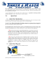
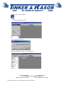
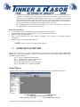
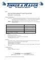
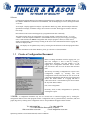
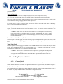
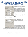
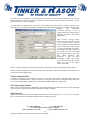
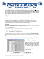
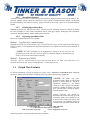
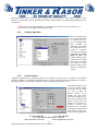
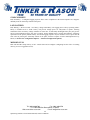
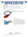
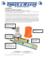
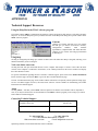
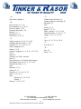
Download DL-1 Old Instructions

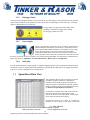
MODEL DL-1 v. 2.0
User Manual
Unpacking Checklist
The Model DL-1 Data Logger Kit includes the following:
Model DL-1 Logging Unit
6A Half Cell Reference Electrode
TRAC Configuration & Analysis Software CD
Carrying Case
9-pin Communications Cable
9-Volt Battery
4-Channel Sampling Interface Cable
Warranty Registration Card
Adapter, Serial Cable to USB port
The information contained in this document is subject to change without notice
and does not represent a commitment on the part of Tinker & Rasor.
All listed trademarks and trade names are the property of their respective
owners.
Any and all reproduction or transmission of any part of this manual, in any form
or by any means and for any purpose other than the personal use by the
purchaser is strictly forbidden without the express written authorization of
Tinker & Rasor.
This manual contains User Information for the Tinker & Rasor Model DL-1 and
the Tinker & Rasor TRAC software package, version 2.
For software updates, please visit our website:
http://www.tinker-rasor.com/software
© 2003 Tinker and Rasor, Inc.
All rights reserved.
011-228
Tel: (909) 890-0700
Fax: (909) 890-0736
P. O. BOX 6890 SAN BERNARDINO, CA 92412
Web: www.tinker-rasor.com
E-mail: [email protected]
i
Sponsoring members of NACE International, NACE Foundation
1.0
Computer Software Setup ...........................................................................1
1.1
Computer System Requirements ................................................................................... 1
1.2
Software Installation ..................................................................................................... 1
1.3
Communication Setup ................................................................................................... 1
2.0
Quick Start ...................................................................................................2
2.1
Quickstart Introduction ................................................................................................. 2
2.2
Quickstart Operation Diagram ...................................................................................... 2
3.0
Feature Summary ........................................................................................6
3.1
Operation Overview ...................................................................................................... 6
3.2
Creating A Configuration Document ............................................................................ 9
3.3
3.4
3.2.1.
Setting Up the Configuration .............................................................................. 10
3.2.2.
Recommended Procedure ................................................................................... 10
3.2.3.
Channel Selections ............................................................................................. 10
3.2.4.
Sequence Parameters .......................................................................................... 11
3.2.5.
Status Section, Configuration Window .............................................................. 12
3.2.6.
Notes & Advanced Options ................................................................................ 12
Communication ............................................................................................................. 12
3.3.1.
Send Configuration ............................................................................................. 13
3.3.2.
Receive Data....................................................................................................... 13
Hardware Setup and Use Overview .............................................................................. 13
3.4.1.
Connecting the Sampling Interface Cable .......................................................... 13
3.4.2.
Data Logger Panel .............................................................................................. 14
3.4.3.
Power Supply ..................................................................................................... 14
3.4.4.
Start/Stop ............................................................................................................ 14
3.5
View Data - Spreadsheet ............................................................................................... 16
3.6
View Data - Graph ........................................................................................................ 16
Tel: (909) 890-0700
Fax: (909) 890-0736
P. O. BOX 6890 SAN BERNARDINO, CA 92412
Web: www.tinker-rasor.com
E-mail: [email protected]
ii
Sponsoring members of NACE International, NACE Foundation
4.0
Feature Details .............................................................................................17
4.1
Status Window .............................................................................................................. 17
4.2
Configuration Options ................................................................................................... 18
4.3
Scaling Inputs & Data ................................................................................................... 19
4.3.1.
Channel Details .................................................................................................. 19
4.3.2.
Sensors & Scaling Methods ................................................................................ 20
4.4
Triggering, Event-based Recording .............................................................................. 22
4.5
Spreadsheet View Features ........................................................................................... 23
4.6
4.5.1.
Scaling Spreadsheet Data ................................................................................... 23
4.5.2.
Spreadsheet Statistics ......................................................................................... 24
4.5.3.
Printing Spreadsheet Data .................................................................................. 24
4.5.4.
Exporting Spreadsheet Data ............................................................................... 24
Graph View Features ..................................................................................................... 24
4.6.1.
Scaling Graph Data............................................................................................. 25
4.6.2.
Graph Statistics................................................................................................... 25
4.6.3.
Printing Graphs ................................................................................................... 26
4.6.4.
Exporting Graphs ............................................................................................... 26
4.6.5.
Formatting Graphs .............................................................................................. 26
5.0
DL-1 Data Logger Unit Operation .............................................................27
6.0
Appendix A: Technical Information ..........................................................29
7.0
Appendix B: Recording and Data Transfer Connections ........................31
8.0
Appendix C: Example of Standard Connection ........................................32
9.0
Appendix D: Technical Support Resources ...............................................33
10.0
Index ..............................................................................................................34
Tel: (909) 890-0700
Fax: (909) 890-0736
P. O. BOX 6890 SAN BERNARDINO, CA 92412
Web: www.tinker-rasor.com
E-mail: [email protected]
iii
Sponsoring members of NACE International, NACE Foundation
1.0
Computer Software Setup
1.1





Computer System Requirement
IBM PC or Compatible, 386 speed processor or better
CD-ROM, DVD-ROM, CD-R or MultiRead CD Drive
8 MB RAM minimum, 16 MB recommended
Windows 95, 98 or newer or Windows NT 4.0 or newer
8 MB available hard disk space
**NOTE: If you do not have a CD drive on the target computer system, a self installing file is
available for downloading from the world wide web. Contact your distributor for the current web
site address.
The DL-1 system is capable of collecting large amounts of data and presenting the information graphically. Because
of this, we recommend that you install the Tinker & Rasor TRAC Configuration and Analysis software on a PC
with a fast microprocessor (200MHz or faster) and at least 16MB of memory (RAM). For information about using
the DL-1 with handheld computers, please see separate PDA User Manual or contact Tinker & Rasor.
Telephone: 626-287-5259
1.2
Software Installation
Insert the installation disk in the appropriate disk drive.
1.
2.
3.
4.
1.3
The CD installation will begin automatically. If the installation program does not open, select Run
from the Start menu and type in or Browse to D:\Autorun\autorun.exe, where D: is your CD drive.
Double click the TRAC Setup icon in the installation window.
Follow the on-screen instructions.
To begin, select the Tinker & Rasor TRAC program from the Start | Programs menu, or double-click
on the trac.exe file from Windows Explorer in the directory where you installed the program (default
directory – C:\Program Files\Tinker and Rasor\trac.exe)
Communication Setup
From the Communication pull-down menu, select
Setup to setup or change the communications port
selection for the PC. At left is the dialog box that
appears. Select the correct COM port or use Auto
Find. Auto Find will find the correct port if the
logging unit is in the “Off” mode, and is connected
to an available COM port on your computer. This
will only need to be done once, unless the PC’s
hardware is changed or a different PC is used.
Tel: (909) 890-0700
Fax: (909) 890-0736
P. O. BOX 6890 SAN BERNARDINO, CA 92412
Web: www.tinker-rasor.com
E-mail: [email protected]
1
Sponsoring members of NACE International, NACE Foundation
Most commonly, COM1 or COM2 is used. For notebook computers, almost always COM1 is used, but on some
older computer models COM1 is used by the Mouse, so you would then use COM2. Rarely is COM3 or COM4
used. A confirmation window appears when Auto Find locates the data logger. Click OK. Click OK again to close
the Communications Port window.
A 9-pin communications cable (null modem cable, included. Please see Appendix B: Recording and Data
Transfer Connections) is used to connect the DL-1 to the host computer.
2.0
Quick Start
2.1
Quick Start Introduction
The Model DL-1 logging unit can sample up to 4 analog channels simultaneously, as fast as 512 times per second or
as slow as one time every 99 minutes, with the capacity to store over 540,000 readings.
The Tinker & Rasor TRAC (True Recording and Capture) Configuration and Analysis software was designed to
be intuitive, so that you can put this capability to work, right out of the box. The “Quickstart Operation Diagram” in
the next section (Section 2.2) shows you how to do this.
By understanding the basic framework of the DL-1 system, you will find that each time you put the system to work,
your experience will not be one of constant “relearning” but one of increasing convenience. Tips are listed in this
introduction and throughout the User’s Guide to help you save even more setup time in future applications.
**Tip: You may use the system for many different applications, or you may use it for the same
application every time. In either case, it will be valuable for you to be able to reuse any work you
have done in the past. The TRAC software gives you the capability to do this by saving
configuration files and sensor profiles. Choose meaningful names for configuration files and
sensor profiles so that you may find them and use them again in the future, either for reference or
for additional data acquisition tasks.
**Tip: Notes can be typed directly into the configuration window for reference. This is an
extremely valuable feature, and the notes are saved and stored to disk along with ALL
configuration settings in data and graph files. In the same way, all raw data that is retrieved from
the logging unit is stored in a graph file. The TRAC software allows you to recreate a
configuration or a complete raw data file, along with scale settings, from a graph file. This
capability makes it easy to organize data and assures that you can always duplicate a setup,
effortlessly.
2.2
Quick Start Diagram
Connect the DL-1 Data Logger to your PC or Handheld computer.
Tel: (909) 890-0700
Fax: (909) 890-0736
P. O. BOX 6890 SAN BERNARDINO, CA 92412
Web: www.tinker-rasor.com
E-mail: [email protected]
2
Sponsoring members of NACE International, NACE Foundation
Open the TRAC software program
Open a New configuration window.
Set the configuration and save.
Send the configuration. The DL-1 is now configured.
Tel: (909) 890-0700
Fax: (909) 890-0736
P. O. BOX 6890 SAN BERNARDINO, CA 92412
Web: www.tinker-rasor.com
E-mail: [email protected]
3
Sponsoring members of NACE International, NACE Foundation
Connect the DL-1 in the field.
Connect the Data Logger in the field using the included
cable with four pairs of clamps. The clamps make it easy to
connect to test stations, like the connection at left between
the DL-1 Data Logger and the Tinker & Rasor CP Test
Station Model T-3.
The DL-1's slim body allows it to slide through the test
station head and hide in the riser pipe. A convenient and
safe location to deploy the DL-1, without having to remove
the test station! You can see the cutout of the test station
terminal marked with an X at left. (This is true for the
Tinker & Rasor Model T-3 CP Test Station. May not apply
to other manufacturers test stations.)
Press the Start/Stop button on the DL-1. The DL-1 is now recording.
The DL-1 has only one button on it:
Start/Stop. All configurations are done
through the computer. This makes the DL-1
the easiest data logger to deploy. Press
Start/Stop and leave. Come back and press
Start/Stop and you are done. (You do not
have to press the button at all if you have
configured a start and stop date/time.)
Retrieve the DL-1 from the field and re-connect it to your PC or Handheld computer.
Connect the DL-1 to your PC using the included cable. The
3-pin (round) end of the cable connects to the DL-1, the 9pin (serial connector) end connects to the computer.
Tel: (909) 890-0700
Fax: (909) 890-0736
P. O. BOX 6890 SAN BERNARDINO, CA 92412
Web: www.tinker-rasor.com
E-mail: [email protected]
4
Sponsoring members of NACE International, NACE Foundation
Open the TRAC software program and the click Receive Data button.
Make sure that the Model
DL-1 Data Logger is turned
off when connected to the
PC or handheld computer.
(No lights are visible on the
face of the Data Logger)
**NOTE: The LED on the
face of the DL-1 will blink
when the unit is recording.
The speed at which the
LED will blink is
configurable to allow for
maximum battery life. To
determine if the unit is
turned off, the LED’s
should be observed for at
least 2 seconds.
View Spreadsheet.
When viewing data in the Spreadsheet window, the
user can see the record number, interval between
reads, value columns and date and time of the read.
It is also possible to hide columns to be able to
focus on just the data you are interested in.
Tel: (909) 890-0700
Fax: (909) 890-0736
P. O. BOX 6890 SAN BERNARDINO, CA 92412
Web: www.tinker-rasor.com
E-mail: [email protected]
5
Sponsoring members of NACE International, NACE Foundation
View Graph.
When viewing the data as a graph, it is possible to
set statistical lines of Minimum, Maximum, Mean,
Standard Deviation and Regression. Also, zooming
in and out of the graph allows you to view all of
the data at once, or just the sequences or individual
reads you wish to view.
Save, print, export.
Spreadsheet data can be exported
as comma separated text for
importing into other spreadsheet
programs, or as xml based for
exporting onto the web.
It is important to note that saving
(exporting) the data into any
format other than the ".dld"
format in the TRAC software
program will allow you to
change the raw data.
Changing is not possible within
the TRAC software program.
Graph data can also be exported
as an image file.
3.0
Feature Summary
Data Acquisition






Stand-alone operation – uses internal memory to store data
Interval Recording
Trigger-based (Event) Recording and Repetitive Triggering
Status Indication: Sampling, Trigger-Mode, Memory Full, Low Battery
Low-Power, Battery Operation
10-year battery backup and software interlock to protect data
Software Framework


The TRAC Configuration and Analysis software framework is compatible with all current level Tinker
& Rasor DL-1 data acquisition systems.
One-button operations to setup the logger, receive data and generate graphs.
Tel: (909) 890-0700
Fax: (909) 890-0736
P. O. BOX 6890 SAN BERNARDINO, CA 92412
Web: www.tinker-rasor.com
E-mail: [email protected]
6
Sponsoring members of NACE International, NACE Foundation


Configurations, data and graphs are treated as documents, much like a word processing program treats
documents. All information is carried forward to the next level ‘document’, which means that you
don’t have to save configurations, data and graphs together as a set – a configuration can be created
from an existing data file or graph file; a data file can be created from a graph file. Once a graph is
created from data collected by the logging unit, the configuration and data files can be discarded, if
desired, for the purpose of storing and organizing data files more efficiently.
The ‘configuration’ button on the status window allows you to create a configuration ‘document’ from
the logging unit that is currently connected to the PC.
Data View & Analysis





View all data or view only the data acquired from individual recording ‘sequences’.
Export/Copy data in table or graphical format to file or directly to any other program.
Print data in table or graphical format.
Print or copy configuration and status window information. This is useful for documenting collected
information.
Statistics may be viewed in table and graph views.
**NOTE: The DL-1 system is Year 2000 (Y2K) compliant.
3.1
OPERATION OVERVIEW
This overview covers the five (5) basic steps involved in collecting and reviewing data. Section 4.0 Feature
Details, covers more advanced features, in addition to instructions for reviewing, formatting and exporting in the
spreadsheet and graph windows.
Step 1: Create a Configuration Document 3.2
Step 2: Communication - Send a configuration 3.3
Step 3: Recording Data - Hardware 3.4
Step 4: Spreadsheet Data View - Receive data 3.5
Step 5: Graph Data View - Generate a graph 3.6
Status Window
The status window (shown on next page) displays the status and specification of the Tinker and Rasor DL-1.
Tel: (909) 890-0700
Fax: (909) 890-0736
P. O. BOX 6890 SAN BERNARDINO, CA 92412
Web: www.tinker-rasor.com
E-mail: [email protected]
7
Sponsoring members of NACE International, NACE Foundation
Inputs
Analog – Four independent channels simultaneously recording AC or DC voltages.
Range selectable: 300 VAC RMS Range or +/- 5 VDC to +/- 100V DC (bipolar).
Range selectable: 1A, 10A and 100 Amps.
Input resolution +/- .01% of selected range.
Channel Configurations:
Channel 1 & 2 – Bipolar DC analog input with automatic AC rejection for data collection and recording
traditionally preformed with a Digital Volt Meter. +/- 5V DC range. Software is configurable
for DC current readings with the appropriate shunt. (see SHUNT Details in table below.)
Channel 3 – 300V AC RMS range.
Channel 4 – Bipolar DC analog input with TrueView. Software configurable for AC current readings with
optional amp clamp.
SOFTWARE CONFIGURABLE SHUNTS
CHANNELS AVAILABLE
.001 Ohm
1&2
.01 Ohm
1&2
.1 Ohm
1&2
1.0 Ohm
1&2
AC Amp Clamp, 0 – 100 Amps
4
Data Storage
Data Storage – 500,000 samples.
Recording Duration: 0.002 seconds to years.
Sampling Frequency: Fast as 500 Hz, Slow as 99 min. (all channels).
Data Memory Battery Life: 10 years.
Operating
Power Supply: 9V battery or adapter. Recorded data retained in memory in the event of 9V-battery failure.
Battery Life: Up to 2 months 9V alkaline, Up to 4 months, lithium.
Temperature Operating: -10 to 60 degrees C.
Temperature Storage: -20 to 70 degrees C.
Status – Led Indication of Logger off/on, Data collection start, Logging stopped/complete, Low battery and
Memory full.
Communication
RS-232 Interface
Baud Rate – 9600 BPS to 115.2k BPS
Tel: (909) 890-0700
Fax: (909) 890-0736
P. O. BOX 6890 SAN BERNARDINO, CA 92412
Web: www.tinker-rasor.com
E-mail: [email protected]
8
Sponsoring members of NACE International, NACE Foundation
Software
Configuration and Data Retrieval from Microsoft® Windows® 95, Windows® 98 or Windows NT® 4.0 or
later, Palm™ handhelds or Palm Powered™ handhelds, such as Handspring™ Visor™, running Palm OS®
3.4 or later.
View Graph – Displays graphs for analysis or presentation. With Copy, Paste, Print and Export functions.
Spreadsheet for display of channel voltage, current and/or event data. Each logged event has a date and
time stamp.
Data collection can be started and stopped by a programmed time/date or manually.
The Status window shows the configuration of a logging unit that is connected to the PC – it is your
“window” to the data acquisition hardware. (Status window shown at top of previous page) If a logging
unit is connected when the TRAC Configuration and Analysis program is started, its status will be
displayed automatically. Other messages relating to the most recent communication with the logging unit
will also be displayed here.
The display can be updated at any time by selecting the refresh button on the main program toolbar.
For more information on the Status Window, please go to Section 4.1: Status Window.
3.2
Create a Configuration Document
Before recording information with the logging unit, you
must first configure it. This is done by creating a
configuration ‘document’ and then sending it to the
logging unit. Configuration documents can be created
once and saved to disk for reuse in future data collection
tasks.
The first step in creating a configuration is to open a New
Configuration template by selecting File
New
Configuration from the main menu. Be sure to select the
configuration template that matches the target logging unit
model. The model number of a logging unit that is
connected to the PC’s communication port can be found at
the top of the Status window.
File New Configuration
Previously saved (to disk) configurations are opened by
selecting File Open.
**NOTE: A configuration document may also be created from a connected logging unit by clicking the
configuration button on the main program toolbar. Configurations can be generated directly from data (.dld) and
graph (.dlg) files by clicking on the configuration icon on the spreadsheet and graph window toolbars.
Tel: (909) 890-0700
Fax: (909) 890-0736
P. O. BOX 6890 SAN BERNARDINO, CA 92412
Web: www.tinker-rasor.com
E-mail: [email protected]
9
Sponsoring members of NACE International, NACE Foundation
3.2.1.
Setting Up the Configuration
Recording parameters (sample interval, run
time, channel selections, etc.) are established
in the configuration. A new configuration is
already initialized with everything necessary
to begin recording – it can be sent to the
logging unit and used, as is. However, you
will want to customize the configuration for
each task.
The configuration window is a “smart form”
that automatically calculates sequence
parameters and displays: 1) the fastest Sample
Frequency possible, and 2) the Total Run
Time that is based on using 100% of the data
storage memory available in the target
logging unit.
These calculations are updated when you
make changes. For example, if you add 3
channels to the default configuration (1 to 4),
the Total # of Samples and Total Run Time
will be reduced by a factor of 4. However,
you can “lock in” a Total Run Time by
clicking the Lock checkbox next to the Total
Run Time field. Similarly, you can “lock in” a
Sample Interval/Frequency by clicking the
Lock checkbox next to that field.
3.2.2.
Recommended Procedure
To appreciate the benefits of the “smart form” feature, specify recording parameters in the following order:
Select each channel to be sampled and enter meaningful channel names.
Set the “Total Run Time” if the test is to be terminated after a specified period of time (though a logging sequence
may be interrupted at any time by pressing the “Start/Stop” button on the panel).
Or
Set the “Total # of Samples” if the test is to be terminated automatically after a specified number of samples have
been acquired.
Set the “Sample Interval/Frequency” – the time base may be changed by selecting the time base button to the right
of the “Sample Interval/Frequency” entry field.
3.2.3.
Channel Selections
Record
The Tinker & Rasor Model DL-1 has 4 analog channels available. Click the checkbox to select the channels that will
be logged during the recording. Use the scroll bar on the right to bring other channels into view.
Tel: (909) 890-0700
Fax: (909) 890-0736
P. O. BOX 6890 SAN BERNARDINO, CA 92412
Web: www.tinker-rasor.com
E-mail: [email protected]
10
Sponsoring members of NACE International, NACE Foundation
Label
After selecting a channel, the cursor will move to the channel name field. You may enter a meaningful name for
each channel, up to 15 characters.
Details
Click on the detail button to access more advanced options for the input channels, such as scaling and triggering
parameters. For more information regarding scaling and triggering, please see Section 4.3.1: Channel Details –
Scaling & Triggering.
3.2.4.
Sequence Parameters
Sample Interval (Frequency)
The default sample rate for a New Configuration is 500 Hz (500 samples per second). The sample rate is autocalculated following entry of other configuration parameters to display the shortest sample interval available.
To set the Sample Interval for a logging sequence, first set the time base by clicking on the
Time-Base Button. Next, type in the desired Sample Interval or Frequency.
The Sample Interval field will automatically “lock” when you modify it, disabling automatic calculation of the
Sample Interval/Frequency.
**NOTE: You may wish to select recording channels and define labels before specifying
sequence parameters. This will enable you to see the automatic calculations for total run time and
total number of samples.
Total Run Time
The Total Run Time parameter allows you to set the duration of a single logging sequence. To automatically
terminate logging after a specified period of time, enter the desired number of days, hours, minutes and seconds in
the respective fields
Auto-calculation displays the Total Run Time that will result when recording from the selected input channels, at the
specified Sample Interval and using all 500,000 data storage locations. When configuration parameters are changed
this field is recalculated, unless it is locked. Total Run Time will automatically “lock” if you enter a value in this
field, or by clicking in the Lock checkbox. The field may be “unlocked” by deselecting the Lock check box.
If the option button to
the left of the “lock” check box is not selected, the Total Run Time parameter is not
enabled. In this case, the Total # of Samples determines the Total Run Time of the sequence, in combination with
the Sample Interval.
Total Number of Samples
The Total # of Samples parameter allows you to define a logging sequence by the number of samples to be recorded.
A sample is defined as a one record of all selected channels. To terminate logging after a specified number of
samples have been logged, enter the desired number of samples in this entry field. Manual entry into this field
“locks” the Total # of Samples parameter, disabling the auto-calculation feature. The field may be “unlocked” by
deselecting the Lock check box.
Tel: (909) 890-0700
Fax: (909) 890-0736
P. O. BOX 6890 SAN BERNARDINO, CA 92412
Web: www.tinker-rasor.com
E-mail: [email protected]
11
Sponsoring members of NACE International, NACE Foundation
If the option button to the left of the “lock” check box is not selected, the Total # of Samples parameter is not
enabled. In this case, the Total Run Time determines the number of samples in the configured sequence, in
combination with the Sample Interval.
3.2.5.
Status Section, Configuration Window
This section indicates the total number of input channels selected for recording. It also displays the percentage of
memory required for the configured logging sequence, and the number of sequences of this particular configuration
that can be recorded with the available data storage memory.
For more information on memory use, please go to the Section 4.2: Configuration Options – Memory Use.
3.2.6.
Notes & Advanced Options
Notes
Select the Notes button to display the “Notes” section of the configuration window. The notes section is convenient
for documenting test setup, special equipment, general explanation of intended uses for the configuration and test
results information to be kept on file for later use. These notes are saved with the configuration so that whenever the
configuration is reloaded from the disk, the test notes will also be available. To view, click the Notes button.
**Tip: This is an extremely valuable feature, when utilized: notes, along with ALL
configuration settings are stored in data and graph files that are saved to disk. In the same way, all
raw data that is retrieved from the logging unit is stored in a graph file when saved to disk. The
TRAC software allows you to recreate a configuration or a complete raw data file, along with
scale settings, from a graph file. This capability makes it easy to organize data and assures that
you can always duplicate a setup, effortlessly.
Advanced
(Please see Section 4.2: Configuration Options – Advanced Configuration Options)
3.3
COMMUNICATION
The DL-1 Logging unit must be in “Off” mode in order to communicate with the TRAC Configuration and Analysis
software through a PC serial communications port. Communication codes sent by the PC will “wake up” the logging
unit each time communication is initiated. A transfer of information takes place between the PC and logging unit for
the following functions:
 Configuration of logging sequence parameters
 Transfer of data to the PC
 Transfer of logging unit status to the PC
 Setting the logging unit’s internal clock
 Personalization of the logging unit with a meaningful name
The first of these functions, configuration and data transfer, are initiated by clicking icons on the main program
toolbar, or by selecting the appropriate sub-menu item under Communications on the menu bar, which are described
below. The remaining communications functions may also be accessed from the main menu and toolbar, and are
described in Section 4.1: Status Window.
Tel: (909) 890-0700
Fax: (909) 890-0736
P. O. BOX 6890 SAN BERNARDINO, CA 92412
Web: www.tinker-rasor.com
E-mail: [email protected]
12
Sponsoring members of NACE International, NACE Foundation
3.3.1.
Send Configuration
**NOTE: If data has been logged but not yet received into a data window, this should be done
before re-configuring the logging unit (see Section 3.3.2: Receive Data).
To send a configuration to the logging unit, be sure the unit is not recording (stopped) and is connected to a serial
(COM) port on the PC with the supplied communications cable. Also make sure that the Configuration window is
the active “window”.
From the Communications menu, select Send Configuration. It takes approximately 10 seconds to send the
configuration and to program the logging unit (use the Communications Setup menu option to change ports if
necessary – see Section 1.3: Communication Setup). Select “OK” at the warning prompt to proceed. The warning
prompt helps avoid accidental loss of data, as this process overwrites the previous configuration and access to
recorded data is lost.
If you have any problems, check to make sure that the Configuration window type (DL-1) matches the logging unit.
The logging unit model number appears at the top of the Status window. If you still have problems, recheck the
cable connection and verify that your COM port is set up properly.
3.3.2.
Receive Data
To receive the recorded data, make sure the logging unit is connected to a serial port on the PC with the supplied
communications cable or to a PDA using Palm OS with optional cable. From the Communications menu, select
Receive Data. While data is being transferred, the progress level is displayed on a meter.
If errors occur while attempting to receive data, make sure that the correct COM port is selected (see Section 1.3:
Communication Setup). Also, make sure the cable is securely connected at both ends.
Once the data is received, a variable-size spreadsheet is created, based on channels configured and the number of
samples recorded. This is the spreadsheet window, which is specially formatted with the channel names that were
specified in the configuration.
3.4
Recording Data – Hardware
This section gives only a brief overview of the DL-1 logging unit and it’s use for recording data. For more detailed
information, please see Section 5.0: The DL-1 Data Logging Unit Operation, or Appendix A: Technical
Information.
3.4.1.
Connecting the Sampling Interface Cable
Connect the 4-channel cable (included in the shipping package) to the connector on the end of the datalogger. The
labeled clips will connect to the equipment being tested. All leads are color-coded and labeled.
Tel: (909) 890-0700
Fax: (909) 890-0736
P. O. BOX 6890 SAN BERNARDINO, CA 92412
Web: www.tinker-rasor.com
E-mail: [email protected]
13
Sponsoring members of NACE International, NACE Foundation
3.4.2.
Datalogger Panel
The panel of the logging unit includes a color legend for the two LED displays. This legend describes the operating
mode associated with each color displayed by each LED and the corresponding text in the same color. A flashing
display is differentiated from a solid color.
*Trigger Mode: The green and orange display flash
alternately to indicate the logging unit is waiting
for the trigger condition to occur.
3.4.3.
Power Supply
The DL-1 logging unit is powered by one (1) 9V battery, and an internal
Lithium battery for data backup. The 9V battery is replaceable. Remove
end cap marked, BATTERY ACCESS, by removing three screws. Insert
battery, observing polarity. The sticker on the inside of the battery
compartment (shown above) shows where the positive terminal on the
battery should be inserted. The battery terminals face INTO the unit when
the battery is inserted. Do not over-tighten screws when replacing BATTERY ACCESS panel. For information on
battery life, please see Appendix A: Technical Information – Battery Life vs. Configuration.
3.4.4.
Start/Stop
Press the Start/Stop button to begin logging. A configured logging sequence will be terminated automatically upon
completion, but may be stopped and restarted manually by pressing the Start/Stop button. The logging unit must be
in the “off” mode for configuration for communications.
3.5
Spreadsheet Data View
This spreadsheet has the same look and feel as popular
spreadsheet programs and data is compatible for
exporting to most Windows platform spreadsheet or
analysis program. For information on scaling, statistics,
printing, exporting, and saving spreadsheet files, please
see Section 4.5: Spreadsheet View Features.
All options are available on the right mouse menu and
also on the main menu bar under Options Data.
Position the mouse over the spreadsheet, click the right
mouse button and the menu will appear.
All functions necessary for viewing or exporting are
available. To select a range of cells, select a corner and
Tel: (909) 890-0700
Fax: (909) 890-0736
P. O. BOX 6890 SAN BERNARDINO, CA 92412
Web: www.tinker-rasor.com
E-mail: [email protected]
14
Sponsoring members of NACE International, NACE Foundation
drag the mouse to the opposite corner. A column or row of cells may be selected by clicking on the column/row
header cell. Click the right mouse button to bring up a menu of choices.
Top and Bottom Rows
Click these buttons to move to the top or bottom rows of the spreadsheet.
“Previous” Sequence and “Next” Sequence
Click these buttons to move the cell cursor to the first row of the next or previous data sequence. These buttons will
have no effect if you are viewing data file that was recorded in a single sequence.
Column otuA -Size
Use this button to automatically size the selected column(s) to the labels and data in view at a given time. This is
normally not necessary but should be used when viewing the cells in the statistics summary – since the information
in these cells is so much wider than is typically in data and label cells, it is sometimes partially hidden to optimize
the spreadsheet view.
Create Graph
A new graph window is generated each time this button is selected. The new graph is a stand-alone “database” that
includes all raw data and configuration information. Refer to the Section 4.6 - Graph View Features for more
information about graphs generated from the Spreadsheet Data View.
Create Configuration (Spreadsheet)
Clicking this button will cause a configuration “document” to be generated from the Spreadsheet Data View
“database”. The spreadsheet has all of the necessary information to construct a duplicate of the original
configuration that was used to record the data.
Data Organization
Data is organized as one row per sample record. Records that represent the time at which recording sequences were
started are color-coded green. The last sample record in a sequence is red. All other records are displayed with black
text. Each sample record consists of three specific column types: Interval, Sample Data and Time Stamps.
Interval
This column displays the actual time of each sample, starting at 0.0 for each recording sequence and increased by
the sample interval value. This column is provided for convenience in creating X-Y charts, as it can be used for “Xrange” data.
Sample Data
These columns display sample data read from the specified input channels – one column per selected channel. The
user-defined channel label is the column name and the ‘engineering units’ are displayed in the first row. Analog data
is displayed as scaled values; by default, 0 to 5 volts.
Time Stamps
The data and time for each data sample are displayed in this column. Data recorded from multiple logging sequences
is displayed sequentially. That is, the first data record in a logging sequence is displayed immediately following the
Tel: (909) 890-0700
Fax: (909) 890-0736
P. O. BOX 6890 SAN BERNARDINO, CA 92412
Web: www.tinker-rasor.com
E-mail: [email protected]
15
Sponsoring members of NACE International, NACE Foundation
last record of the previous sequence. The start of a new sequence is easily distinguished by the green-colored text, in
addition to the 0.0 value in the Interval column.
3.6
Graph Data View
**NOTE: Various formatting options are available on the right mouse menu. Access this menu
by placing the mouse over the graph window and clicking the right mouse button.
“All: Sequences Method”
Click this toggle button ‘on’ to view all recorded sequences as they were on continuous of paper. Each sequence
starts right after one another, end-to-end. The x-axis values will reset and count up for each sequence. When viewing
the graph this way, the next and previous sequence buttons have no effect. The Graph Start button moves to the
beginning of the 1st sequence. The Graph End button moves to the end of the last sequence.
“Individual” Sequence Method
Click this toggle button ‘on’ to view each
sequence individually in the graph
window. The scroll bar at the bottom will
scroll from the beginning of the current
sequence to the end of the current
sequence. If you want to view other
sequences, click the next and previous
buttons. This current sequence is displayed
on the tool bar.
Graph “Beginning” and “End”
Click these buttons to move the graph view
to the beginning of the 1st sequence, or the end of the last sequence regardless of the current graph method. If you
are viewing multiple sequences and want to move to the beginning of a particular sequence, use the scroll bar.
Graph “Next” and “Previous” Sequence
Click these buttons to move between sequences.
Zoom “In” and “Out”
Click this button to zoom in on the data by a factor of 2. The center of the graph window is the zoom point.
Open Data View (Spreadsheet)
Click this button to show the spreadsheet data view.
Tel: (909) 890-0700
Fax: (909) 890-0736
P. O. BOX 6890 SAN BERNARDINO, CA 92412
Web: www.tinker-rasor.com
E-mail: [email protected]
16
Sponsoring members of NACE International, NACE Foundation
Create Configuration (Graph)
Use this option to open the configuration form with the parameters used to generate this data. This allows you to
quickly configure a logging unit from a previous test file because all options are duplicated from the original
configuration.
4.0
Feature Details
This section will discuss in detail some of the advanced features of the TRAC Configuration and Analysis software
program.
4.1
Status Window
For general information about the Status Window and its function, please refer to the Section 3.1: Operation
Overview – Status Window.
The status of the device currently connected to the communication port is displayed in the status window. (See
graphic in section 3.1, Status Window)
A tool bar is displayed at the top of the main program window. Certain tools on the toolbar are used to communicate
with devices connected to the communication port. Clicking the right mouse button while the cursor is over the
status window will also bring up the menu of available communications functions.
Name
The logging unit may be personalized for
identification. This is especially useful when
more than one DL-1 is in use for the same or
similar applications. The name can have up to 15
characters and may contain any keyboard
character.
The current name is listed at the top. It is also
initially placed in the edit field. To change the
name, just enter a new name (up to 15 characters)
and then press the OK button.
Clock
The logging unit contains a real-time clock. Use this option to change the time and date.
The PC’s current date and time are the default values placed in the edit fields. To synchronize the DL-1 logging
unit’s internal clock to the PC, just select “OK”. Any other valid setting may be entered, as well. The DL-1 system is
Year 2000 (Y2K) compliant.
Tel: (909) 890-0700
Fax: (909) 890-0736
P. O. BOX 6890 SAN BERNARDINO, CA 92412
Web: www.tinker-rasor.com
E-mail: [email protected]
17
Sponsoring members of NACE International, NACE Foundation
**NOTE: The time is in 12-hour format (AM
or PM must be specified) and the date is
month/day/year (2-digit year). This software
recognizes the years “00” and up to be the years
2000 and up, so there is no concern for Y2K
problems.
Refresh
When the program first starts up, it determines if
there is a logging unit connected, and if so, it will
display the status. At anytime you can press the
Refresh button to get the most-up-to-date status of
whichever device is connected.
Contents of the Status Window
The Status window is a direct link to the DL-1
logging unit. Information displayed here resides
in memory within the logging unit, including; date and time of configuration, number and name of input channels
selected, configuration parameters and available memory. If there is more information than space provided, scroll
bars will appear to permit full viewing.
The status window is updated each time communication is established between the PC and the logging unit.
4.2
Configuration Options
Memory Use
Each analog channel requires 1 memory storage location (500,000 storage locations are available for sampled data).
Selecting all 4 analog channels would use 4 storage locations each time the inputs are sampled.
Advanced Configuration Options
Advance Configuration options are accessed
from the Advanced button located in the
Status section of the Configuration window.
Logging Indication Flash Interval
The Logging Indication Flash Interval is the
rate at which the Light Emitting Diode
(LED) indicator flashes (green) while the
logging unit is in the Logging mode.
**NOTE: Advanced options control the
general operation of the logging unit,
affecting battery life and behavior following
Tel: (909) 890-0700
Fax: (909) 890-0736
P. O. BOX 6890 SAN BERNARDINO, CA 92412
Web: www.tinker-rasor.com
E-mail: [email protected]
18
Sponsoring members of NACE International, NACE Foundation
power interruptions.
Theory of Operation
Typically, the LED flashes each time a sample is logged; however, if the sample interval is very
fast, .05 seconds or less, the LED will stay on constantly while the logging unit is in the logging mode.
With slower sample intervals this method of indication is less useful, as minutes could pass before a flash. For this
reason, a method of forcing a “logging indication flash” is provided.
For sample intervals of one (1) second or longer, the LED will flash at a rate which is the faster of the Sample
Interval or the Logging Indication Flash Interval.
For example, if the sample interval is 5 minutes, and the flash interval is 10 seconds, the LED will flash every 10
seconds, even though samples are being logged at 5-minute intervals. The indication is more meaningful if it is
frequently visible.
**NOTE: If this value is “0”, the LED will not flash at all. Use this option to conserve battery
power. Faster flash rates will reduce battery life. The “0” mode functions only when the sample
interval is one (1) second or greater. When faster sampling is involved, memory capacity will limit
run time, rather than life.
Power Interruption Recovery Mode
When this option is selected, logging will resume following a power interruption. If this option is not selected, a loss
of power will terminate recording – logging will not resume when the supply voltage returns to the normal operating
level.
Timed Start Mode
When this option is selected, logging will start at the time and date entered. In the first field enter the year, month
and day. In the second field enter the time in 24 hour format (1 P.M. = 13:00). In the third field enter “1” for the
Timed Start to be enabled. Enter “0” to disable the Timed Start Mode.
**NOTE: When the DL-1 is configured to start at a preset time, pressing the Start/Stop button
will not start data logging on the DL-1. Instead when the Start/Stop button is pressed, the
“Logging” LED will flash three times to indicate the DL-1 is programmed to start at a later time.
4.3
Scaling Inputs and Data
4.3.1.
Channel Details
“Channel Details” are optional parameters that can be used to further customize an input channel.
Options include scaling the input voltage to engineering units, such as degrees Celsius, and defining an input or
group of inputs as a “trigger”.
The Channel Label can be changed for the input channel that is currently displayed in the Channel field at the top of
the window. Any change made here will be reflected in the Configuration window.
Tel: (909) 890-0700
Fax: (909) 890-0736
P. O. BOX 6890 SAN BERNARDINO, CA 92412
Web: www.tinker-rasor.com
E-mail: [email protected]
19
Sponsoring members of NACE International, NACE Foundation
The Input Range normally will not change. Select 0 to 5
volts if you have the standard Model DL-1 logging unit.
The input range is the basis for scaling calculations and
it is important that the correct range is specified.
Scaling can be accomplished by applying a defined
sensor “profile” to the input channel that is currently
displayed in the Channel field at the top of the Channel
Details window. Once this window is displayed, any
analog input channel can be scaled by first selecting an
input channel and then the desired sensor to apply.
Click the Scaling button to review or change scaling
parameters or to define new sensor profiles. This
process is described in Section: 4.3.2: Sensors &
Scaling Methods.
Triggering parameters are set in the Trigger Setup
window. Bring up this window by clicking the
Triggering button. The trigger setup process is
described in Section 4.4: Triggering, Event-Based
Recording.
4.3.2.
Sensors & Scaling Methods
**IMPORTANT: Care should be taken
in naming, modifying and deleting sensor
profiles as this will affect the interpretation
and presentation of preexisting data and graph
files that use these sensor profiles. Sensor
profiles that have been applied to input
channels and indexed by unique sensor names,
and changing the scale parameters provide
more information related to sensor profile
management.
In order to scale an input channel to engineering units,
a sensor profile with the desired scale parameters must
be applied to that channel. Sensor profiles are created
and ‘managed’ in the Scaling window. This window, in
combination with the files that store the profiles, forms
a sensor profile database. This database is ‘managed’
by adding, changing or deleting sensor profiles.
A sensor name is used as a reference to identify the scaling equations needed to support scaling an individual sensor
output to meaningful units. Once you have entered an equation for scaling, you now only have to reference it by
name.
Use the Scaling dialog box to define new scaling equations if the scaling equations you need are not already defined.
For convenience and brevity, sensor profiles will be referred to as “sensors”.
Tel: (909) 890-0700
Fax: (909) 890-0736
P. O. BOX 6890 SAN BERNARDINO, CA 92412
Web: www.tinker-rasor.com
E-mail: [email protected]
20
Sponsoring members of NACE International, NACE Foundation
Two sensor types are available: 1) user-defined sensors that can be created deleted or modified, and 2) factory
defined sensors that cannot be modified or deleted. User-defined sensors are preceded by an asterisk (*) in the
sensor name field, for easy identification.
A sensor cannot be added with the same name as an existing sensor. Each sensor must have a unique name,
consisting of at least one different character. Though you may not be recording the input of a sensor at all, the sensor
database
and
management
convention provides a way to
organize and reuse scaling profiles,
trimming keystrokes from future
applications.
Add a sensor by typing a unique
name in the Sensors: field at the top
of the Scaling window, and then
click the Add button once the desired
scale parameters have been entered.
You may find it helpful to first select
an existing sensor that is similar to
the desired new sensor. You should
then change the name in the sensor
field before modifying scale
parameters so that you don’t
accidentally “update” the original
sensor. However, this will not occur
unless you click on the Update
button, specifically.
Delete a sensor by making it the currently selected sensor in the Sensors: field, and then click the Delete button.
Modify a sensor by making it the currently selected sensor in the Sensor: field. Then, change the scale parameters as
needed, and click the Update button.
2 Points Scaling Method
To define a scale using the 2-point method, you may use any 2 known values for converting the input signal (volts)
to the desired engineering units (i.e. degrees Celsius). You will get the best results by using the 2 known values that
are closest to the Input Range extremes (0 to 5 volts for the standard Model DL-1 logging unit).
Zero-Span Scaling Method
Many sensors are shipped from the manufacturer with scaling information provided in the form of a Zero and a Span
value. To use this method, select Zero-Span and fill in the fields accordingly.
Slope/Intercept
Signal or Sensor characteristics may be understood in the form of a line equation, y=mx + b, where ‘m’ is the Slope
and ‘b’ is the Intercept. Choose Slope/Intercept to use this method of scaling.
Tel: (909) 890-0700
Fax: (909) 890-0736
P. O. BOX 6890 SAN BERNARDINO, CA 92412
Web: www.tinker-rasor.com
E-mail: [email protected]
21
Sponsoring members of NACE International, NACE Foundation
Sensor Database
Sensor database files have the “.sen” extension and are located in the same directory as the Tinker & Rasor TRAC
software. Care should be taken so that these files are not damaged or deleted. If you perform regular backups to
protect information on your computer you should include these files, but make sure that you are always using the
latest version.
4.4
Triggering, Event-Based Recording
Enable Trigger
Other than using the Start/Stop button on the logging unit, you can use the trigger mode, causing a recording
sequence to begin when a specific “event” occurs. To use this event-based recording mode, click The Channel
Details button in the Config window. In the Channel Details window, you will see the Triggering section. To use
the Trigger feature, uncheck the Disable all triggering box.
Analog
The Analog option allows you to trigger recording when an analog input exceeds a specified threshold. In addition,
you can specify the trigger to occur when the signal is increasing or decreasing when it crosses the threshold.
Behavior is similar to the trigger feature of most oscilloscopes.
Single Sequence/Repetitive
Each trigger method requires that
the trigger is first “armed”. That
is, in order for the trigger
condition occur, the inputs must
first be in a state other than the
trigger condition. In order to
trigger when a state match occurs,
the inputs must first be in a nonmatching state - specifically, for
at a time period of at least 1
millisecond (0.001 second). This
is partly to avoid Repetitive
Triggering during the same
“event”. To trigger when an
analog input rises above 1 volt, it
must first be below 1 volt.
The trigger feature in the DL-1
can be used in two ways: Single
Sequence or Repetitive.
Select Single Sequence to record
only at the first occurrence of the
event. This will start recording
when an event threshold is
reached. Once this threshold has
been reached, the DL-1 will
continue recording until either the
memory is full, of is a lock is
Tel: (909) 890-0700
Fax: (909) 890-0736
P. O. BOX 6890 SAN BERNARDINO, CA 92412
Web: www.tinker-rasor.com
E-mail: [email protected]
22
Sponsoring members of NACE International, NACE Foundation
placed on the # Samples or Run Time and those limits are reached, as set in the main Config window.
Repetitive triggering is very similar to Single Sequence with one important difference. If Run Time is locked in the
main Config window, the DL-1 will start recording when an even threshold has been reached and stop recording
when the total Run Time has been reached. If the Threshold level drops below the Edge (either Low to High or High
to Low), the DL-1 will “re-arm” itself, and continue to watch for the threshold edge once more. When the threshold
edge is reached again, the DL-1 will start recording until the Run Time is again reached. This behavior will repeat
until the memory is full, the instrument is manually turned off or the battery is depleted.
Trigger Channel
The Trigger Channel does not have to be input that is selected for recording. Select any channel to be the trigger
input. Only one Channel can be a trigger.
Sensor
The trigger input can be scaled. Use a sensor from the sensor database to define the scale and then specify the
threshold in terms of the scale for that sensor. If a compatible sensor is not available, the sensor must first be
created. This can be done from within the Channel Details box. You can get the Channel Details box from the
Configuration window. The Sensor field only applies with the Analog trigger method.
Threshold
Specify the desired threshold for the trigger event to occur. The valid range and units are displayed to the right of
this field. The Threshold field only applies to analog trigger methods.
Low to High, High to Low
Select the polarity of the trigger event here. This parameter does not apply to State triggering.
4.5
Spreadsheet View Features
For general information on using the Spreadsheet View, please refer to Section 3.5: Spreadsheet Data View.
Additional features are described here that relate to formatting, analyzing, printing and exporting of spreadsheet
data.
All options are available on the right mouse menu and also on the main menu bar under Options | Data. Position the
mouse over the spreadsheet, click the right mouse button and the menu will appear. (As shown below)
4.5.1.
Scaling Spreadsheet
Data
Data records that appear in the Spreadsheet
window can be scaled in the same way as the
logging unit input channels are scaled prior to
recording data. Each column of data is treated
as a “channel” and scaled as described in
Section 4.3: Scaling Inputs & Data. The
Channel Details window contains only the
fields that apply to the Spreadsheet View, but
has a similar format as when selected from the
Configuration window.
Tel: (909) 890-0700
Fax: (909) 890-0736
P. O. BOX 6890 SAN BERNARDINO, CA 92412
Web: www.tinker-rasor.com
E-mail: [email protected]
23
Sponsoring members of NACE International, NACE Foundation
4.5.2.
Spreadsheet Statistics
A statistical summary of data recorded from each input channel is displayed at the bottom of the spreadsheet. The
statistical quantities include: Minimum, Maximum, Average (Mean), Standard Deviation-Sample, and Standard
Deviation-Population. The statistical summary applies to all data in the current “sheet” for the associated channel
column.
4.5.3.
Printing Spreadsheet Data
4.5.4.
Exporting Spreadsheet Data
Highlight the desired cells, and select File | Print…from the menu bar. Additional options are available for printing
the entire spreadsheet, in color, border, and gridlines and for setting page margins. Printing the entire spreadsheet
includes the statistical summary and the channel names and labels.
Data can be exported using either of two methods:
Method 1 – Copy Directly to Another Program
Highlight the desired cells, and select Edit | Copy from the menu bar or Copy from the right mouse button pop-up
menu (or Control C). In the application to which the information is to be copied, select Paste from the edit menu (or
Control V).
**NOTE: The entire spreadsheet can be highlighted by clicking in the top left cell in the
spreadsheet (just to the left of the “Interval” label). The statistical summary is included when you
do this, as are all of the channel names and labels.
Method 2 – Export as an ACSII File
Select File | Save As…from the menu bar. In the File Type field, choose *.txt. Enter a file name with a “.txt”
extension and click on “OK”. Select a column delimiter – Comma, Space or Tab.
4.6
Graph View Features
For general information on using the Graph View, please refer to Section 3.6: Graph Data View. Additional
features are described here that relate to formatting, analyzing, printing and exporting of graph data.
**NOTE: The graph view offers
presentation quality output for copying and
printing – in color or black ink – but can be
significantly degraded by the limited
resolution of most monitors and graphics
controllers. Though the display may look
poor, especially when viewing 3D graphs,
the print should be crisp.
Selected, commonly used features are
described in this section, but many powerful
presentation features are available and can
be discovered by exploring the options with
a real data file. All formatting options are
available on the right mouse menu (click the
Tel: (909) 890-0700
Fax: (909) 890-0736
P. O. BOX 6890 SAN BERNARDINO, CA 92412
Web: www.tinker-rasor.com
E-mail: [email protected]
24
Sponsoring members of NACE International, NACE Foundation
right mouse button and the menu will appear) and also on the main menu bar under Graph | Options. Several
features are worth noting, such as 3D plotting and rotating, placing images on a graph, adding background colors
and gradients.
**Tip: To rotate a 3D graph, hold down Control+Shift, click the left mouse button wherever you
want a “handle” on the graph, and then drag the mouse.
4.6.1.
Scaling Graph Data
Data records that appear
in the graph window can
be scaled in the same
way as the logging unit
input
channels
are
scaled prior to recording
data. Each data series is
treated as a “channel”
and scaled as described
in Section 4.3: Scaling
Inputs & Data. The
Channel Details window
contains only the fields
that apply to the Graph
View, but has a similar
format as when selected
from the Configuration
window.
4.6.2.
Graph Statistics
A graphic representation of a statistical summary can be applied to any data series, or “channel”. The statistical
quantities available are: Minimum, Maximum, Mean (Average), Standard Deviation and Regression (“best-fit”
linear approximation). These statistical quantities apply to the data that is currently in view.
The Statistics options can be
accessed by double clicking
on the data series for which
you want to apply the
statistic formula, or by
clicking the right mouse
button and selecting Series,
Series Type, and the desired
channel (series) name. The
Statistics tab will then be
available, as shown in the
dialog box above. The result
of Minimum, Maximum and
Mean applied to a data series
is shown in the graph below
Tel: (909) 890-0700
Fax: (909) 890-0736
P. O. BOX 6890 SAN BERNARDINO, CA 92412
Web: www.tinker-rasor.com
E-mail: [email protected]
25
Sponsoring members of NACE International, NACE Foundation
represented by dotted and dashed lines.
4.6.3.
Printing Graphs
Make sure the graph window is active and select File | Print… from the menu bar. Options are available on the Print
dialog box for: 1) layout, and 2) fitting the graph to the paper. The default options have been set to those that are
most widely used, and generally give good results.
**Tip: Do not resize the ‘plot” area of the graph by dragging the mouse. This indicates a manual
“fix” of the graph size and disables optimal scaling of the graph to the printer page size. If you
wish to enlarge the graph for viewing on the screen, try maximizing the graph window first.
Additional options are available for centering the graph on the printer page and setting page margins.
4.6.4.
Exporting Graphs
Graphs can be exported using either of two methods:
Method 1 – Copy Directly to Another Program
Make sure the graph window is active, and select Edit | Copy from the menu bar or Copy from the right mouse
button pop-up menu (or Control C). In the application to which the information is to be copied, select Paste from the
edit menu (or Control V).
**NOTE: Many programs offer options for pasting, usually if you select Edit | Paste Special…
in the target program before pasting. The TRAC program exports the graph in three formats that
may be used by another program; Metafile, Bitmap and JPEG. The metafile is generally preferred
when you wish to be able to resize the image and retain high quality fonts and graphic
components, since it is vector-based. Bitmaps allow for editing images at the pixel level, and can
be used in programs that do not accept vector-based images. JPEG format is useful for images that
will be placed on the web or e-mailed.
Method 2 – Save as an Image File
Select File | Save As… from the menu bar. In the File Type field, choose Metafile, Bitmap or JPEG. Enter a file
name with the appropriate extension and click on “OK”.
4.6.5.
Formatting Graphs
Graph objects (axis scale, data series, footnote, and titles) can be formatted by double clicking on the object. Some
useful, but not so obvious, features and methods are described here to get you started.
Tel: (909) 890-0700
Fax: (909) 890-0736
P. O. BOX 6890 SAN BERNARDINO, CA 92412
Web: www.tinker-rasor.com
E-mail: [email protected]
26
Sponsoring members of NACE International, NACE Foundation
Format Chart Options
Position the mouse over the graph window and click the right button. Select Chart Designer. Options include the
display format for the title, footnote, legend and second Y-axis on the current chart. From tree view in the left panel
of this dialog you can also format any other feature of the chart.
Plot On 2nd Y-Axis
When viewing more than one data series and the magnitude of the scaled data differs greatly, one signal may be “in
the dirt” or out of view, depending on how the Y-axis is scaled. It may be helpful to plot one or more data series on
the 2nd Y-axis, so that two scales can be used. To do this, double-click on any data series to pop up the Chart
Designer with the Options tab selected for that particular data series. Then select Plot on 2nd Y-Axis.
Format Axis/Scale
To change the scale of an axis, double-click on the axis to pop up the Chart Designer with the Scale tab selected for
that particular axis.
5.0
DL-1 Data Logger Unit Operation
The panel of the logging unit includes a color legend for the two-color LED display. As seen below, this legend
describes the operating mode associated with each color displayed by the LED. A flashing display is differentiated
from a solid color.
OFF
No display – the logging unit is currently idle. This is the state the DL-1 should be in when connected to a computer.
START
Green, momentary – a logging sequence has been initiated from the “Start/Stop” button on the panel.
LOGGING
Green, flashing – currently sampling (see Section 4.2: Configuration Options – Advanced Configuration
Options, for more information).
Tel: (909) 890-0700
Fax: (909) 890-0736
P. O. BOX 6890 SAN BERNARDINO, CA 92412
Web: www.tinker-rasor.com
E-mail: [email protected]
27
Sponsoring members of NACE International, NACE Foundation
STOP/COMPLETE
Red, momentary – a configured logging sequence has to run to completion or the current sequence has “Stopped”
manually from the “Start/Stop” button on the panel.
LOW BATTERY
Red, flashing, ½ Hz for seconds – low battery; change immediately. The logging unit is always operating when a
battery is installed. Even a “dead” battery will provide enough power for subsystems to operate, allowing
notification of the low battery voltage condition for some time. A sufficiently discharged battery may not give the
full 10-second indication. Please note that a separate, built-in lithium battery protects Data Memory. Following
replacement of the primary alkaline battery, the current logging sequence may be continued. Loss of power has the
same effect as pressing the “Start/Stop” button on the panel, with the exception of Power Interruption Recovery
Mode (see Section 4.2: Configuration Options – Advanced Configuration Options).
MEMORY FULL
Data and time/date stamp memory is full - transfer data and re-configure (configuring has the effect of resetting
memory; access to logged data is lost).
Tel: (909) 890-0700
Fax: (909) 890-0736
P. O. BOX 6890 SAN BERNARDINO, CA 92412
Web: www.tinker-rasor.com
E-mail: [email protected]
28
Sponsoring members of NACE International, NACE Foundation
APPENDIX A
Model DL-1 Technical Information
1. Battery Life Vs. Configuration
Battery life is virtually independent of the number of channels configured for sampling. With 1 channel selected,
540,000 sample records can be logged, but with 4 analog channels selected only 135,000 sample records can be
logged.
For short run times, power consumption is not critical. However, with long run times in applications which require
battery operation, it is important to verify that the configuration will run to completion before the battery is drained.
The following graph shows the effect of variations in the Logging Indication Flash Interval with various Sample
Intervals at room temperature.
The Sample Interval directly affects battery life; each sample recorded consumes a fixed amount of power. To be
sure a logging sequence will run to completion before battery power is expired, find the desired logging sequence
Total Run Time on the “Battery Life (Days of Life)” axis on this chart. A horizontal line drawn through this point
will intersect the curves for various Sample Intervals, indicating valid combinations of the sampling and flash
Tel: (909) 890-0700
Fax: (909) 890-0736
P. O. BOX 6890 SAN BERNARDINO, CA 92412
Web: www.tinker-rasor.com
E-mail: [email protected]
29
Sponsoring members of NACE International, NACE Foundation
intervals for which a Duracell 9V Alkaline battery Vs. a Lithium battery at full capacity will provide proper
operation.
**IMPORTANT: This profile for battery life does not apply when the Trigger Mode is enabled.
With trigger mode enabled, battery life is much shorter. The actual life is not to be specified because of
the many options and unknown trigger frequency. Estimated operating times for a 9V alkaline battery
range between 15 and 30 hours in the trigger mode.
2. Timing and Storage Format
The sequence in which input channels are sampled follows the order shown in the application software configuration
window, starting with Channel 1 and ending with Channel 4.
Each analog channel to be sampled requires approximately 200 microseconds. Actual sampling is completed after
12 microseconds (this is the “sampling time aperture”); however, some time is required for conversion and filtering.
Four (4) of these samples are taken and then averaged for each reading to be recorded.
3. Electrical & Mechanical Specifications
INPUTS
Analog
Input Voltage Range
Resolution
Absolute Accuracy
Input Bias Current
4 Analog
0 to 5 V (DL-1-10:0 to 10V)
20mV (DL-1-10:40mV)
± 10mV (DL-1-10 ± 20mV)
400 nA (DL-1-10: ~ 15k )
Sampling Frequency
Fast as 512 Hz, Slow as 99 min. (All channels)
DATA STORAGE
Data Storage
Recording Duration
Data Memory Battery Life
540,672 samples
0.002 seconds to years
10 years
OPERATING
Power Supply
Voltage
Current
Standby
Recording
LED Indication (sampling)
9V battery
300 A
BATTERY LIFE
26mA (only while sampling)
10mA (can be disabled)
Up to 1 month, 9V Alkaline(up to 2 months, lithium)
Temperature
Operating
Storage
0 to 60 degrees Celsius
-20 to +70 degrees Celsius
COMMUNICATION
RS-232 Interface
Baud Rate
Connection
Data Format
DIMENSIONS
WEIGHT
115,200 bps
9-pin female
8 data, no parity, 1 stop bit
1 ½ in. X 1 ½ in. X 10 ¼ in.
8.4 OZ. (237 G)
Tel: (909) 890-0700
Fax: (909) 890-0736
P. O. BOX 6890 SAN BERNARDINO, CA 92412
Web: www.tinker-rasor.com
E-mail: [email protected]
30
Sponsoring members of NACE International, NACE Foundation
APPENDIX B
Appendix B: Recording and Data Transfer Connections
The Model DL-1 includes cables necessary for data recording and data transfer. The cables are distinct and easily
identified.
Data Collection Cable (Sampling Interface Cable)
The Data Recording cables have a serial connector at one end and
four pairs of color-coded and labeled clamps at the other end.
Data Transfer Cables
The Data Transfer cable included with the Model DL-1 is a
serial cable with a 9-pin connector at one end and a 3-pin
round connector at the other. The round connector (3-pin)
is always attached to the Model DL-1 and the serial
connector (9-pin) is always attached to the computer. You
can leave the Data Transfer cable attached to your
computer when not in use, and you can attach and detach
the DL-1 to the Data Transfer cable without having to turn
your computer off. (May not apply to all computer
operating systems)
Tel: (909) 890-0700
Fax: (909) 890-0736
P. O. BOX 6890 SAN BERNARDINO, CA 92412
Web: www.tinker-rasor.com
E-mail: [email protected]
31
Sponsoring members of NACE International, NACE Foundation
APPENDIX C
Example of Standard Connection
Connecting the DL-1 to the Tinker & Rasor Model T-3 Test Station
Below is an example of a common connection using the Model DL-1 Data Logger. This example connection is
made using a Model T-3 CP Test Station from Tinker & Rasor.
The Black lead from the Channel One pair of leads connected to the DL-1 is clamped to the terminal board of the T3, which in turn is connected to the buried pipeline (not shown). The Red lead of the Channel One pair is connected
to the included Model 6A Half-Cell Reference Electrode, which is then used to obtain a reading from the ground.
After connection, the DL-1 is either started manually by pressing the Start/Stop button, or left to start recording on
its own according to its programming. Depending upon the configured sampling time, the technician will wait for
the sample to complete or return to retrieve the data. The data may be retrieved in the field using a laptop computer
or a handheld device such as a Handspring ™ running Palm OS™ software, or the DL-1 can be removed and
brought to a desktop computer unit for downloading of data. (See Appendix B: Recording and Data Transfer
Connections for more information about the included and optional cables used with the DL-1.)
Channel 1:
Connected to T-3 Test Station.
(assumed T-3 connection to
buried pipeline)
Model T-3 CP Test Stations.
Sold separately.
Channel 1:
Connected to included
Model 6-A CuCu/SO4
reference electrode.
Model 6-A CuCu/SO4
Half Cell Reference
Electrode. Included
with the DL-1 Kit
Model DL-1 Data Logger
Version 2 Hardware.
Four-pair Data Collection Cable
attached, using Channel 1 pair,
with booted clamps (red / black).
Tel: (909) 890-0700
Fax: (909) 890-0736
P. O. BOX 6890 SAN BERNARDINO, CA 92412
Web: www.tinker-rasor.com
E-mail: [email protected]
32
Sponsoring members of NACE International, NACE Foundation
APPENDIX D
Technical Support Resources
Using the Help files in the TRAC software program
The Tinker & Rasor TRAC Configuration and Analysis software program has help menus, a help index and many
help files. To access the Help files, point your mouse and click on the Help menu along the top of the window in the
TRAC software program.
Contents
Clicking on Contents will bring up a new window
that will give you choices of Overview, Glossary,
Configuration
Window,
Data
Window
(Spreadsheet), Graph Window and Status Window.
Clicking on any of these will bring up information
on that subject.
Using Help
Clicking on Using Help will bring up a window of choices that will outline how Help is designed, and help you to
find the information you are looking for.
Visit www.tinker-rasor.com
Clicking this link will open the default browser on the computer and attempt to connect to the Tinker & Rasor
website. If the computer is connected to the Internet, or has a dialup connection, the browser window will display
the Tinker & Rasor website.
For specific information regarding the DL-1 and DL-1 technical support, please click on the Product Instructions
link on our home page, and click on DL-1 to get to the DL-1 Product Instructions page.
The DL-1 Product Instruction page on the Tinker & Rasor website has a Frequently Asked Questions (FAQ) page,
an area of technical support resources, the latest TRAC software version available for downloading, and contact
information for technical support.
About
Clicking About… will show you the TRAC software splash screen and the version number. This is important to
note, as you may be asked for the version information of the TRAC software program you are using if you contact
Tinker & Rasor Technical Support.
Contacting Technical Support
Technical Support E-mail
[email protected]
Hours of Operation: 8am - 4pm, M-F
Pacific Time
Telephone:
Facsimile:
+1 (909) 890-0700 (US)
+1 (909) 890-0736 (US)
Tel: (909) 890-0700
Fax: (909) 890-0736
P. O. BOX 6890 SAN BERNARDINO, CA 92412
Web: www.tinker-rasor.com
E-mail: [email protected]
33
Sponsoring members of NACE International, NACE Foundation
INDEX
--0-9-9-pin, cable, i, 1, 4, 26, 27
15-pin, cable, i, 4, 26, 27
Formatting Graphs, 23
Frequency, 7, 8, 9, 26
--G--
--A--
Graph Data, 5, 6, 13, 21
Acquisition, data, 2, 5, 7
Advanced, configuration, 6, 9, 10, 14, 16, 24
Analog, channel, 2, 6, 7, 9, 13, 16, 17, 19, 25,
26
Auto-size, column, 13
--H--
--B-Battery, i, 5, 7, 12, 16, 24, 25, 26
Battery Installation, 12
--C-Cable(s), i, 1, 3, 4, 11, 27, 28
Channel, details, 9, 17, 19, 20, 21
Channel(s), analog, see Analog, channel
Clock, set, 11, 15
Column, 4, 12, 13
Communication,
configuration, 1, 10
cables, 27
Configuration Window, 3, 8, 10, 16
Configuring, channels, 7, 9
Connecting, 11, 28
Copy, 6, 8, 20, 21, 22
--D-DL-1, operation, 23
Data Transfer, 1, 11, 27, 28
Details, channel, See Channel, details
Display, LEDs, 12, 23
--E-Enable, See Trigger
Event-Based Recording, 17, 19
Exporting, 5, 6, 12, 20, 21, 22
--F--
Half Cell, See Reference, electrode
Handspring™, i, 7, 27, 28
Help, 28
--I-Input Range, 7, 17, 18
Interval, See Sample, interval
--K-Logging, See Sequence, logging
Logging Indication Flash Interval, 16, 25
--L-Label, 9, 11, 13, 17, 20, 27
Lock, 8, 9, 10, 11
--M-Minimum, Maximum, Mean, 5, 20, 21, 22
--N-Name, Set/Change, 11, 15
Notes, 2, 10
--O-Options, advanced, 9, 10, 16
--P-Palm OS, 7, 11, 28
Panel, 9, 12, 23, 24
PDA, 1, 11, 27
Power supply, 7, 12, 26
Printing
Graph, 21, 22
Spreadsheet, 20
Ranges, 20
Formatting, 6, 13, 20, 21
Tel: (909) 890-0700
Fax: (909) 890-0736
P. O. BOX 6890 SAN BERNARDINO, CA 92412
Web: www.tinker-rasor.com
E-mail: [email protected]
34
Sponsoring members of NACE International, NACE Foundation
--Q--
--T--
Quick Start, diagram, 2
Technical Specifications, 26
Technical support, contacting, 28
Threshold, 19
Time
Setting, 11, 15
Stamp, 7, 13, 24
TRAC, software, 2, 4, 5, 10, 18
Transferring data, 1, 4, 10, 11, 27
Trigger, 5, 9, 12, 17, 19, 26
--R-Receive data, 4, 5, 6, 11
Recording data, 6, 11, 20, 21
Recovery Mode, 16, 24
Reference Electrode, i, 28
Refresh, 7, 15
Regression, 5, 21
Run Time, 8, 9, 16, 25
--S-Sample, interval, 8, 9, 10, 13, 16, 25
Sampling Interface Cable, i, 11, 27
Scaling, 9, 12, 17, 18, 20, 21, 22
Send, configuration, 11
Sensors, 17, 18
Sequence, logging, 6, 8, 9, 10, 13, 14, 23, 24,
25, 26
Slope, 18
Software, see TRAC, software
Span, 18
Specifications, see Technical Specifications
Spreadsheet, data view, 6, 12, 13, 14, 20
Standard Deviation, 5, 21
Start
Manually, 12, 23
Setting, 16, 17
Statistics, 6, 12, 13, 20, 21, 22
Status, 7, 10, 14, 15
Stop
Manually, 12, 16, 17, 24
Setting, 7
Storage, 7, 8, 10, 16, 26
--V-View, 4, 5, 12, 13, 14, 20, 21
--Y-Year 2K, 6, 15
--Z-Zero, 18
Zoom, 5, 14
Tel: (909) 890-0700
Fax: (909) 890-0736
P. O. BOX 6890 SAN BERNARDINO, CA 92412
Web: www.tinker-rasor.com
E-mail: [email protected]
35
Sponsoring members of NACE International, NACE Foundation