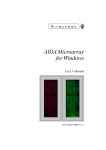
1
2007 Edition
AGScan
USERS MANUAL
Version 0.2 / July 2007 Edition
Nicolas Mary && Rémi Cathelin
Copyright © 2006 SIGENAE / INRA
Permission is granted to copy, distribute and/or modify this document under the terms of the GNU Free
Documentation License, Version 1.2 or any later version published by the Free Software Foundation;
with the Invariant Sections being just "Background", no Front-Cover Texts, and no Back-Cover Texts.
A copy of the license is included in the section entitled "GNU Free Documentation License" at the end
of this manual.
AGScan v0.2 User Manual
page 1
2007 Edition
Revision table :
Version
Date
Major modifications
Author(s)
0.1
February 15 2006
First release
R. Cathelin
0.2
July 18 2007
Color parameters menu
Customizer for default algorithm buttons
Generic image opening
Generic batch
N. Mary
th
th
Acknowledgment :
I wrote this guide in English having the aim to give access to AGScan to the largest possible scientific
community. But English is not my mother language, so any remark about the orthography or the
grammar is welcome.
AGScan v0.2 User Manual
page 2
2007 Edition
INDEX
INTRODUCTION .................................................................................................................................................4
MAIN FEATURES OF AGSCAN.....................................................................................................................................4
VOCABULARY...........................................................................................................................................................4
GENERAL OVERVIEW.......................................................................................................................................5
THE PROCESS ..........................................................................................................................................................5
FILE FORMATS..........................................................................................................................................................6
IMAGE QUALITY........................................................................................................................................................6
INSTALLING AGSCAN ON YOUR COMPUTER..................................................................................................................7
Download.........................................................................................................................................................7
packages contents............................................................................................................................................9
Launching AGScan..........................................................................................................................................9
PROCESSING STEPS ........................................................................................................................................10
USER INTERFACE ....................................................................................................................................................10
CHOOSE COLOR CONFIGURATIONS..............................................................................................................................12
LOADING AN IMAGE FILE ..........................................................................................................................................13
CREATING A GRID...................................................................................................................................................16
ALIGNING A GRID ON AN IMAGE.................................................................................................................................18
Loading a grid...............................................................................................................................................18
aligning manually a grid...............................................................................................................................19
Global alignment algorithm..........................................................................................................................21
Local alignment algorithm.............................................................................................................................23
Shortcut buttons.............................................................................................................................................26
Spot detection.................................................................................................................................................26
THE TABLE ...........................................................................................................................................................27
QUANTIFYING AN ALIGNMENT ..................................................................................................................................28
quantifications...............................................................................................................................................28
analyze your results.......................................................................................................................................30
Export results.................................................................................................................................................31
PROCESSING A BATCH..............................................................................................................................................33
Batch tab........................................................................................................................................................33
Preparing the batch.......................................................................................................................................34
Save/Open a batch..........................................................................................................................................37
PLUGINS..............................................................................................................................................................38
PRESENTATION........................................................................................................................................................38
EXAMPLE: THE “MEMORY PLUGIN”..........................................................................................................................38
FREQUENTLY ASKED QUESTIONS.............................................................................................................40
INDEX...................................................................................................................................................................41
WORD INDEX ........................................................................................................................................................41
ILLUSTRATION INDEX...............................................................................................................................................43
GNU GENERAL PUBLIC LICENSE................................................................................................................45
AGScan v0.2 User Manual
page 3
Sigenae
February 2006 Edition
Introduction
This manual is aimed to provide the necessary information to biologists using AGScan image
processing software. The document is split in four parts :
• Introduction
• General overview
• Processing steps
• Plugins presentation
• Frequently asked questions
A bit of history
AGScan is a micro-array image processing software developed by the SIGENAE team.
http://www.sigenae.org/
It is an evolution of BZScan : BZScan is a radioactive DNA micro-array image processing software
based on the JAI library . It was developed by the TAGC (http://tagc.univ-mrs.fr/ ) from 2002 to 2005.
In 2005, the SIGENAE team decided that it was worthwhile to go on with the development of BZScan,
and mainly by going through the new Sigenae version named AGScan.
This software is freely available using the following address:
http://mulcyber.toulouse.inra.fr/projects/agscan/
You can also download the source code, report bugs and propose enhancements at the same
address.
Main features of AGScan
The main features of AGScan are :
1. Grid conception
2. Able to use single or multiple ( up to 3) channel images as input
3. Image manipulation and processing based on ImageJ
4. Manual and automatic global alignment
5. Automatic local alignment
6. Automatic quantification
7. Batch processing
8. Data export
9. Plugin support, to add new file formats, alignment or quantification methods...
10. Multi-language support
These different features will be presented in the rest of this document.
Vocabulary
Image : is a file produced by a micro-array scanner and sometimes modified (cut,...).
Grid : is first a file generated by AGScan describing the way the array has been spotted. From this it
can be aligned on an image and be a part of an alignment. You will see later the importance of the grid
structure.
Alignment : is composed of an image and a grid. It can have several states like 'not aligned', 'globally
aligned' and 'locally aligned'.
Quantification : once the alignment is finished the quantification is the process of extracting one or
more figures for each spot giving an intensity value for the spot.
Batch : is a group of alignments processed by AGScan from global alignment to quantification through
local alignment.
AGScan User Manual
page 4/45
Sigenae
February 2006 Edition
General Overview
This chapter presents an overview of the whole process, some information about image file types and
quality and gives the software install procedure.
The process
To start the process you need at least :
• a micro-array image (different formats can be used),
• a grid file (generated in AGScan see next chapter section),
• AGScan installed (see install procedure below)
Notice that AGScan works with 16bits-unsigned grayscale images.
By default, AGScan input image format is the TIFF format but ISAC format (INF/IMG) is also
recognized by a plugin automatically provided into all AGScan versions.
The grid file can be generated with AGScan or provided by someone having generated it. To share a
grid you have to be sure that the micro-array and the definition used to scan the image are the same.
The process can be split in five steps :
- experiment image(s) loading
- grid loading
- global alignment : This step can be done by
AGScan or by the user. It corresponds to the
general alignment of the designed grid on the
image(s).
- local alignment : This step is done by AGScan.
Starting from the global alignment AGScan tries
to figure out what the small local changes are to
fit the sub-grids as well as possible to the image.
- quantification : This step is done by AGScan.
Starting from the local alignment coordinates
AGScan calculates for each spot several
quantification values. These values will be
presented later on.
Image(s)
Grid
Glocal Alignment
Local Alignment
Quantification
As presented before, AGScan is able to process an image and a grid without any human help. This is a
very important and user asked AGScan feature.
AGScan User Manual
page 5/45
Sigenae
February 2006 Edition
File formats
AGScan can load and save several file formats depending on the element. See table hereunder.
Element
image
1
grid
experiment:
Alignment
quantification
batch
file extension
comments
.tif
Standard format of compression of image
without loss of information,
.inf
This file is the information file of the
corresponding “.img” file. Both files have to be in
the same directory to be used by AGScan. This
file type is named ISAC and is for example
produced by the Fuji BAS5000 scanner.
.grd2
This file type is produced and used by AGScan.
The format is kind of XML compliant.
/ .zaf
.bzb4
This file type is produced and used by AGScan.
It's an archive file that contains a “.ali” file
(experiment data file), a manifest file and may
contains the image(s), The “.ali” format is kind of
XML compliant.3
This file type is produced and used by AGScan.
The format is kind of XML compliant.
Notice that AGScan provides also non-openable export formats like a “.txt” output, easily usable with
your favorite spreadsheet.
Image quality
Even if AGScan proposes methods for automatically align grids on image, the result depends of a lot
of things like the quality of the image, the grid structure and parameters used for the alignment.
1- Be aware that the image files have to be a 16 bits format to be processed by AGScan.
2- Be careful: BZScan and AGScan .grd grid files and .bzb batch files are incompatible!
3- Never try to open a .zaf file: .ali files are not alone support
4- Be careful: BZScan and AGScan .grd grid files and .bzb batch files are incompatible!
AGScan User Manual
page 6/45
Sigenae
February 2006 Edition
Installing AGScan on your Computer
Download
AGScan is freely available at:
http://mulcyber.toulouse.inra.fr/projects/agscan
Just click on the “Files” subsection:
Mulcyber AGScan page
AGScan User Manual
page 7/45
Sigenae
February 2006 Edition
All versions of the software are available. They are named using the date of the release.
The software releases are available in two different packages: light and full versions. With the light
version, Java Runtime Environment needs to be installed previously on your operating system. The full
version does not need any other software, just to click on the icon!
Downloading AGScan is very easy.
First choose a release of the package. For each release, notes are available by clicking on the release
name.
Next you can download the corresponding “AGScanxxxxxx.zip” file.
Release notes
Download link
Download AGScan
packages contents
AGScan User Manual
page 8/45
Sigenae
February 2006 Edition
The “AGScanFullxxxxxx.zip” archive file contains the following directory:
The “AGScanLightxxxxxx.zip” archive file contains the following directory:
Package contents are similar except 3 elements added to the Full version:
– the install directory: contains a Java Runtime Environment
– the “AGScan.cfg” file: the launcher configuration file
– the “AGScan.exe” file : the icon to launch AGScan (on Windows OS)
Note: the Full version launcher is only usable for Windows OS.
The file structure of files is composed of:
– the “AGScanxxxxxx.jar” file is the java executable archive file
– the languages directory containing language files available in AGScan
– the “lib” directory containing AGScan libraries and dependences used by the
software (ij.jar for example). Notice that the subdirectory called “plugins” of this
directory contains imageJ plugins that can be used by AGScan
– the “plugins” directory containing AGScan “.class” plugins files
– the “ChangeLog.txt” file containing the history of release notes
– the “parameters.properties” file containing the current user preferences of the
software
Launching AGScan
On Linux OS, use the command line:
java -Xss10m -Xmx420m -jar AGScanxxxxxx.jar
On Windows OS:
If you choose a full version: just click on the AGScan.exe icon!
You can also run the command line (or write it in a .bat file):
"java.exe" -Xss10m -Xmx420m -jar "AGScanxxxxxx.jar"
The “.jar” file name is the release name of AGScan.
Note: the “-Xss” and the “-Xmx” parameters correspond to the memory allocation given to the Java
Virtual Machine(JVM) in order to support the application. If you encounter “java OutOfMemory errors”
then increase the “-Xmx” value.
By default, AGScan full version is configured with 420Mo of memory allocated for the JVM.You can
modify this value in the launcher configuration file (“AGScan.cfg”file).
AGScan User Manual
page 9/45
Sigenae
February 2006 Edition
Processing steps
This guided tour will walk us through the different parts listed hereunder :
– User interface,
– Loading an image file,
– Creating a grid,
– Aligning a grid on an image,
– The table,
– Quantifying an alignment,
– Analyzing quantification results,
– Processing a batch.
First it will start by presenting the user interface layout:
User interface
AGScan Title
Toolbar
Menu bar
Display
window
Status bar
The user interface of the software wants to be simple, readable and as ergonomic as possible.
It is composed of five elements:
– The “title window”: presenting the used AGScan version, in the selected language.
– The “menu bar”: containing the different menus of the application.
– The “toolbar”: icons wich are shortcuts to some sub-menu actions.
– The “display window”: the main window containing experiment view. Several
elements may be displayed in the same time (images, grids, alignments). They are
open in different tabs.
– The “status bar”: displays current information like status and progress bar.
AGScan User Manual
page 10/45
Sigenae
February 2006 Edition
As we want the software to be simple to use we tried to place the menus in a logical order from left to
right. We hope that menus are explicit enough to be easily memorized. Shortcuts to common actions
have been added below the menus in order to open, align and quantify an image in three clicks!
Shortcut icons are also duplicated next to each menu title to ease memorization. Notice that if you
point your mouse on a shortcut, you will obtain a little description of the associated action.
Example : the “Open Image” action menu (and related toolbar item)
The first menu you can use is the “Edition>Language” one. It allows to change the language of the
application menus.
Notice that you need to reload the application to apply a new language.
Note: in the current version, three languages are available: English, French and German.
There can be spelling mistakes. However it is easy to modify these faults. Indeed, all the words are
stored in text files (named “messages_en.properties”, “messages_fr.properties” and
“messages_de.properties”). We can even easily generate new ones in other languages. For that, it is
necessary to add the new “messages_xx.properties” file into the subdirectory of AGScan named
“languages”. It will be automatically recognized by the software.
Now Let us present the different steps needed to quantify an image.
AGScan User Manual
page 11/45
Sigenae
February 2006 Edition
Choose color configurations
A menu is available to setup the number of channels and their names for the opening of image.
Use “Edition->Color Parameters” to access this menu.
First, you need to choose a number of configurations
(between 1 and 6). Then click on “Validate” to update
the window.
Now, you see a number of text fields equal to your
previous choice.
It's time to setup the configurations.
configuration must have the following syntax :
Each
N:Color1,Color2,Color3,...
N is the number of channels you want. For example if
you want to setup a configuration for opening 4channels images, you will enter :
4:Color1,Color2,Color3,Color4
Illustration 1: 4 configurations
Color1 to Color4 are the channel name.You are
totally free to choose them. For example, you could
choose like in the left picture :
4:Violet,Blue,Green,Yellow
Once, you have choose the configurations you want
you can click on “Ok” to save your choices.
If you mistake unfortunately, and have less or more
configurations than you want, you could change the
value in the “Number of parameters” panel and click
“Validate” to reupdate the window.
You must specify a number of configurations at
least equal to 1.
You must fill all the fields before clicking on
“OK”.
You can't setup two or more configurations with
the name number of channels.
Illustration 2: 2 configurations
AGScan User Manual
page 12/45
Sigenae
February 2006 Edition
Loading an image file
Preliminary remark: an experiment can be composed of as much images as you want , but in the
following chapters we will refer to a few experiments including one and two images only.
To open an image, use the “File>Open>Image” menu or the following short icon of the toolbar:
A selection window appears. Choose your type of
experiment specifying the image number of
channels and then clicking on “Validate” to
update the window.
Notice that you can only choose a number of
channels that refers to a color configuration. The
default configurations available are :
1:P33
2:Cy5,Cy3
So if you want to open images with more than two
channels, don't forget to use “Edition->Color
parameters” (cf. 0.9 Choose color configurations).
Once you validate, you will be able to browse for
each channel file of the image.
Notice that only the images files extensions that
AGScan supports are visible in the file chooser,
(By default “.tif” and “.inf”).
The “Properties” button allows you to give some
initial parameters of the image (produced by the
scanner). These parameters are stored into the
general parameters of the application.
-Pixel width : width of a pixel, micrometers
-Pixel height : height of a pixel, micrometers
-Unit: image unit (QL or PSL)
-IP type: Image Plate size ,centimeters
-Latitude: dynamic range of “above number”
power of 10
If you don't know where to find these parameters,
ignore them (default values will be apply).
Click “OK” to load the experiment!
AGScan User Manual
page 13/45
Sigenae
February 2006 Edition
The image is loaded into the “Display window”.
In the case of a multi-channels experiment, the RGB image is displayed :
AGScan User Manual
page 14/45
Sigenae
February 2006 Edition
Once opened, you can now modify it using the different widgets disposed in the “Image” menu.
They allow to invert the LUT, to modify the contrast and the
brightness, to rotate the image, to flip it horizontally or vertically.
Some of these options are very interesting when you have
scanned your array the wrong way. You can also select a
rectangular region and crop it to create a new sub-image.
Sometimes due to low contrast or quality, the spots can be quiet
difficult to locate. All these image tools can help you to visualize
them. However, you have to know that the modification of the
contrast and the brightness of the image doesn't affect pixel
values of the image and isn't save.
Other general functionalities can be used in the “Display” menu.
An example: the “zoom”:
Working with images, we sometimes need a general view and sometimes a very precise one. This can
be obtained by using the zoom . Clicking on the left of the progress bar will zoom out of the image,
clicking in the right will zoom in the image.
When the zoom is active, the icon background becomes gray. By clicking a second time on the icon,
the zoom is disable.
Example: image with zoom action enabled.
AGScan User Manual
page 15/45
Sigenae
February 2006 Edition
The “display” tools are :
- “tabs” or “windows”: the display mode. Each item (image, grid,
alignment) is on a tab or on a distinct window, Tabs are the
default display mode.
- “zoom”: disable/enable the zoom,
- “zoom window”. Allows to display a little window containing the
entire image, the zoom factor applied and that show the part of
the image zoomed.
- “Display the ruler”: disable/enable a ruler. Disabled by default.
- “Display the State bar”: disable/enable the status bar. Enabled by
default.
-”Properties”: allows to display the properties (name,size...) of the
current element displayed into the current tab or window.
By default, the display mode is “tabs”, the zoom isn't active, the ruler is disabled and the status bar is
displayed. (see the image above).
On this example, the window mode is active,the status bar is hidden, the ruler is displayed and the
zoom window is open (the current zoom factor is 3),
The next part will show you how to create a grid.
Creating a grid
The grid is a very important element for the image analyze. After opening an image, you have to load a
grid on it and therefore you must have already define it.
Note that you can use the same grid for all your experiments that use the same spotting scheme.
So this part will show you how to create, open and modify a grid.
AGScan User Manual
page 16/45
Sigenae
February 2006 Edition
At first, choose the creation grid menu found in the “File>Create>New Grid” menu or in the “Grid>New
Grid” menu.
A new tab and the “structure editor” will appear. The main window is divided into two parts:
– the grid: the graphical representation of the grid
– the table: a table with all the characteristics of the grid spots (number, name position). It will be
describe later.
By default, the editor appears on a “one level” grid, So we have to introduce you the notion of level in
the grid. A grid can have two levels representing the block and the grid.
–
level1 = the block level. In fact, the spotting is usually made using a block pattern. This is usual but
not always the case. The level defines a block of spots. Information needed is the dimension of a
block (number and size of columns and lines) and the diameter of a spot.
–
level2 = the grid level. A grid can often be compared to a set of blocks. So if you have this second
level, you just need to inform how many blocks you have vertically and horizontally. So you can
also notify inter-blocks space size.
To sum up, a grid is seen by AGScan as a set of elements. The smallest element is the spot. When
you have two levels, a set of spots forms a block and a set of block a grid .
AGScan User Manual
page 17/45
Sigenae
February 2006 Edition
In the next table the first line gives you number of levels used, the second gives you the structure of
the first level and the third line gives you the structure of the second level. In the last line, you can see
the graphical view of the type of spotting pattern you have used.
1 level
2 levels
2 levels
20 x 12 spots
12 x 12 spots
1 x 1 spots
-
4 x 2 blocks
10 x 10 blocks
Examples of grids
The grid, the table and the editor are linked. So, be aware that you need to move on an other box or hit
<ENTER> (carriage return) after having entered a value in each text box of the “grid structure editor” in
order to synchronize the view of the grid .
You have now define your grid and you can save it. The default proposed name of the saved file has
no sense. It is just created randomly in order to be unique.
The resulting file has a “.grd” extension and is in XML format.
Notice that you cannot create a grid directly on a loaded image. You need before to load the image and
after the grid above.
Aligning a grid on an image
Loading a grid
This is where all really begins. After having opened an image, you can load a grid on it.
To do this, you can use the “Grid>Load” menu or the following icon :
The selected grid will be loaded on the image, placed on the top left and the tab is divided into two
parts, in order to add the table of spots characteristics.
AGScan User Manual
page 18/45
Sigenae
February 2006 Edition
The next step consists in correctly aligning the grid on the image.
You have several possibilities to do it. This step can be done manually or automatically by launching
alignments algorithms.
All the alignment functionalities are available in the “Alignment” menu:
aligning manually a grid
How to manually place the grid?
You can either use the mouse and the “Move/Rotate/Resize” menu.
Let us present to you the “color code” of a grid: a loaded grid on an image appears in blue if it is not
selected and orange if you select it.
To select in the grid, just click on it.
Note that you can easily only move a sub-grid by changing the selection mode:
These three icons of the toolbar allow to change the grid selection mode. By default, the first is
enabled. It corresponds to the entire grid. If you select the second icon, you turn into the block mode
that allows you to only select a block. The third icon corresponds to the spot mode that allows to only
select one spot.
AGScan User Manual
page 19/45
Sigenae
February 2006 Edition
A selected item (spot, block or the grid) can be moved using the mouse. For this, move it by
maintaining it selected (left mouse button down).
Notice that the table view corresponding selected spots lines are yellow.
Block selection mode
Spot selection mode
Here
You can also deform the grid by placing your mouse at the corners and drag them.
A specific and useful tool allow to easily manually align a grid :the “Move/Rotate/Resize” menu.
Click on it: a window appears, offering you the possibility to rotate, move and resize the grid of given
values:
Example: the grid has been moved and rotated.
You can choose the unit of your rotation (degrees, radian), the unit of your translation or resizing
(pixels, µm or spots).
Thanks to this tool, you can manually correctly place the grid on the image. In order to verify the
position of each spot, you can apply a “spot detection” (presented below).
Note that it is possible to perform an automatic local alignment on a manually aligned grid.
AGScan User Manual
page 20/45
Sigenae
February 2006 Edition
It is interesting to know how manually place a grid but in the most cases, you can perform automatic
global and local alignments.
In the next pages we will see how to perform these automatic alignments.
Let us first introduce the notions of “global” and “local” alignments. The global alignment places the
grid (as good as possible) on the entire image. The local alignment searches to correctly align each
block separately.
These two algorithms have been initially developed for the BZScan software. So they have a lot of
parameters that can be modified and memorized.
Global alignment algorithm
The “Global alignment” sub-menu contains two different algorithms, the “sniffer” and the “edges
detection” global algorithms. The default algorithm is the “sniffer” one (in bold in the menu). You can
also call it thanks to the following toolbar icon :
If you click on “Default algorithm”, it is launched without proposing you to change the parameters. To
modify them, you need to choose the “Sniffer” menu. So the parameters windows appears:
AGScan User Manual
page 21/45
Sigenae
February 2006 Edition
Notice that all these parameters can be changed and saved. It is also always possible to restore the
default parameters. So don't hesitate to change them. For more information about their meaning,
please contact us.
“Sniffer” algorithm quick presentation:
At first, the angle of the image is calculated. Then (about 10% of the process), the algorithm try to
parse all the image with a sniffer block to find all spots. To do this, it already searches to place the
“sniffer block” (a defined block of spots) at 40% in width and in height of the image, the condition to
place it is that the center spot must be a detected one. When the algorithm detects this spot, it
considers this position as the first position of its route (pict1). The sniffer block moves after in all the
direction of the image and flags every spot it finds. Each time it will find something considered a spot, it
will put a little colored cross on its center (pict2). After having recovered the entire image, the algorithm
computes how to place the grid in order to include the most of detected spots.
At the end of the process, you will have a yellow (selected) grid aligned on the image(pict3).
The Sniffer block
Spots are found
Grid is placed
Some visual steps of the sniffer global alignment.
Our grid is now globally aligned.
The next step of the process is the local alignment.
Local alignment algorithm
A local alignment is an alignment that you must launch on a “already aligned” grid. It allows to improve
the alignment quality.
In the actual version, two different local alignment algorithms are available.
The “Local alignment” sub-menu contains two different algorithms, the “entire grid” and the “block by
block” local alignment algorithms. The default algorithm is the “block by block” one (in bold in the
menu). You can also call it thanks to the following toolbar icon :
AGScan User Manual
page 22/45
Sigenae
February 2006 Edition
If you click on “Default algorithm”, it is launched without proposing you to change the parameters. To
modify them, you need to choose the “Alignment block by block” menu.
“Alignment block by block” algorithm quick presentation:
Each block is processed individually. The position of each spot is verified and adjusted. The block may
be moved from the initial global alignment place.
Progression of the local algorithm
In this process, AGScan takes each block and tries to fit it as precisely as possible to the spots it finds
underneath. Each block is processed separately and can therefore move from the previously
calculated global position to a new one. It is quiet amazing to see how a block is progressing towards
its end position. Once the block position is optimized, AGScan goes on with the next block.
The red circles indicate that the program identify a spot ; on the opposite, the green ones indicate that
the spot is deduced due to the grid structure and the red spots locations.
Note that the coordinate values of the spots have changed during the local alignment process. You can
see values in the alignment table.
The progress of the alignment is given by a progress bar.
At the end of the process your display windows will look like this :
AGScan User Manual
page 23/45
Sigenae
February 2006 Edition
An aligned grid
AGScan User Manual
page 24/45
Sigenae
February 2006 Edition
Shortcut buttons
In the toolbar, you can see an icon like this one :
This icon permits to customize the two following icons :
Here is the selection window that opens when you click on it :
You can choose the default algorithm to use for global alignment and local alignement here.
As you can see on the previous picture, “Move it 2!” and “Sigenae Global Alignement” are plugin
algorithms. In fact, if you own some global alignement plugins, there are dynamically add to the
selection box.
Spot detection
The spot detection is the method used to define if a spot is found (red) or estimate (green). A spot is
recognize as one if its form fit the model.
You can call it on a selected a grid. Indeed, a selected grid becomes orange, so you don't see the
spot nature.
The “Spots detection” sub-menu contains two different algorithms, the “2 profiles” and the “4 profiles”
algorithms. The default algorithm is the “4 profiles” one (in bold in the menu). You can also call it
thanks to the toolbar icon :
If you click on “Default algorithm”, it is launch without propose you to change parameters. To modify
them, you need to choose the “4 profiles” menu.
The “2 profiles” and the “4 profiles” spot detection algorithms are similar. The difference is that profiles
of spots used to search the center of the spot since the center of the research zone are diagonal lines
(for the “2 profiles” detection) and diagonals + vertical + horizontal lines (for the “4 profiles” detection).
AGScan User Manual
page 25/45
Sigenae
2 profiles
February 2006 Edition
4 profiles
These two methods progress rapidly and give you the percentage of detected spot in the status bar:
The table
When a grid is open, the main window is split into two parts, giving you access to a table view of the
spot informations.
This table is synchronized with the alignment. So coordinates have been updated by the move of the
grid. However, no new columns are added.
A selected spot and its table description
Base columns are:
– the first column is the number of the spot, determined by the spotting plan.
– Name: ID of each spot defined by AGScan: the first part is the block ID, the second part is the spot
ID. The letter corresponds to the line position (A,B.....) and the number is the column position
(1,2,3,,,).
– X : X coordinate of the center of the spot in the image(in micrometer).
– Y : Y coordinate of the center of the spot in the image(in micrometer).
– R: row number in the entire grid.
– C: column number in the entire grid.
– Block: number of the current block.
– Row: row number in the current block.
– Column: column number in the current block.
– Diameter: constant diameter of the spot defined in the grid structure.
Note: the “Computed diameter” column is present but not used (values are “-1”) until the quantification
is processed.
AGScan User Manual
page 26/45
Sigenae
February 2006 Edition
The table and the alignment are interactive. You can select a spot in the table and see its location at
the same time on the alignment: the spot (or the set of spots) are highlighted into the alignment (see
the figure above).
So it's also possible to sort columns values, copy it,color some values...
The columns options can be active by clicking on the right click of the mouse.
The interest of these options will be describe to you after the quantification part.
Quantifying an alignment
Now you have an aligned grid. So the next step is the quantification.
quantifications
Several computations are available. To launch a quantification, use the “Quantification>Compute”
menu and select your action.
You can choose the type of quantification you want to call or select several of them with the “Selection”
sub-menu or the following toolbar icon:
AGScan User Manual
page 27/45
Sigenae
February 2006 Edition
The selection menu opens the next window:
Here, you can choose the classic AGScan columns you want to process.
Alternatively, you can choose a quantification plugin in a list.
All installed plugins appears in the plugin list, and this list is dynamically generated (for example, if you
install a new quantifiaction plugin, it will be added to the list).After selecting the actions you want to
process, click on “OK”.
Each calculation is done one after the other. You can follow advance thanks to the progress bar.
Results are available into the table.
Example of columns added, results of quantifications
Note: the “Computed diameter” column is filled during quantifications that need this value.
By selecting the data column title, you can change its position in the table.
Available AGScan Quantifications:
Four quantification are available in AGScan:
– Image/Constant diameter Quantification: for each spot,the quantification value is computed thanks
to the image pixels intensities and the constant diameter given by the grid structure.
– Image/Variable diameter Quantification: for each spot, the quantification value is computed thanks
to the image pixels intensities and a variable computed diameter.
– Fit/Constant diameter Quantification:the quantification value is computed thanks to the estimated
intensity of the spot (with a fit function) and the constant diameter given by the grid structure.
– Fit/Variable diameter Quantification: the quantification is computed thanks to the estimated
intensity of the spot (with a fit function) and its variable computed diameter.
AGScan User Manual
page 28/45
Sigenae
February 2006 Edition
The QM value is an indication of quality of the spots. Each spot has a value of QM ranging between 0
and 1 (the closer the value is to 1, the more it is reliable).
The “fit correction” and the “overshining correction” are two corrections values that can be used with
quantification. Be careful, to apply them, you need a specific formula.
analyze your results
Thanks to the table columns options, you can sort the result values,
Example of a sorted column: click right on the column header and choose “Sort> Descending Order”.
An useful option is also the “color” tool. You can choose to give a color to some spots of the alignment
in order to locate them.
Example: we want to color in orange spots that have an “image/constant” quantification value higher
than 10000. To do that:
1/select the “Modify” menu of the “Qtf Image/Const” column.
2/Check the “superior” case, fill the value (10000) and choose a color(orange).
"Modify a column" window
AGScan User Manual
page 29/45
Sigenae
February 2006 Edition
3/Click on “Apply” and “Close”,
4/select the “Color spots” menu of the “Qtf Image/Const” column.
The text header of the column becomes red. Spots concerned by this condition will appear in orange
on the aligned image.
In our example, only 4 spots are colored (as the sorted column shows us before).
Spot coloration example
You can also color spots between two values or lower than an other one.
Export results
You can save the experiment in every process step. An alignment and a quantification are considered
as the same thing. In fact, there are two “aligned grid with a table”. Only tables columns differ. So use
the “save” menu to save it. The extension of an experiment file is “.zaf”.
You can also export only the table values in order to use them into a spreadsheet.
To do that, select the menu:
"Quantification>Export>Text File" menu
The file saved content looks likes:
AGScan User Manual
page 30/45
Sigenae
February 2006 Edition
Text file output example
Now, you have done a complete analyze of your image.
Do you know that this process can also be repeat automatically, using the batch mode?
AGScan User Manual
page 31/45
Sigenae
February 2006 Edition
Processing a batch
Batch tab
A batch allows to analyze automatically several experiments!
Important note: all these expermiments are analyzed with the same grid.
To create a batch, you can use the “File>Create>New Batch” menu or the “Batch>New Batch”.
The associated icon of the toolbar is:
The batch tab contains two parts:
Left part
Right part
"Batch" tab
The tab is split into two parts, the right part that displays experiments status and images open and the
left part that contains the configuration of the batch.
AGScan User Manual
page 32/45
Sigenae
February 2006 Edition
Preparing the batch
Batch files configuration
In the top of the left part of the tab:
1/ Choose if the batch will work alignments or not (images).
1bis/ If you choose to process a batch working with images, select the number of channels for images.
2/ Click on the grid browse button and select the grid.
3/ Choose the output directory where results will be saved.
4/ Check or not the fact to save image into the archive created for each image. Notice that if the image
isn't in the archive, you need to give its localization when you will open the experiment.
5/ Click on “Add Images” to select images.
Note: you can add images one by one or several in the same time in a multi-selection (only in “1
channel mode”).
After choosing several images: the right part is filled:
Batch experiment information
You can now choose all the actions you want to process for each image thanks to the job leftpart.
AGScan User Manual
page 33/45
Sigenae
February 2006 Edition
"Batch" parameters configuration
You just need to select the process you want in the two top lists and click on “Add” .
The added processes appear in the bottom list.
You must choose exactly one global alignement or/and one local alignment, and one quantification,
else you won't be able to launch the batch.
Moreover, two options are available and could be added or not in any case :
•
The snapshot mode : takes a photo of each alignment and save it in a jpeg file.
•
The export results mode : save the quantification result in a text file.
If you mistape and add a process you do not want, you can select it and click on “Remove” to erase it
from the bottom list.
To launch the batch, just click on “Launch”. Following a "Batch" in progress
AGScan User Manual
page 34/45
Sigenae
February 2006 Edition
When the batch starts, you can stretch the bar at top to follow the batch in progress.
The status of each image is updated.
In the statusbar of AGScan, the total percentage of the batch is given.
When the process is successfully finished, the image status is “DONE”.
Batch progress finished
When the batch is finished, you can see results in the output directory.
For each experiment, you will have:
– the archive .zaf file
– the snapshot .tif file (rapid snapshot of the alignment, optional)
– the export files (optional)
In our example, we have analyze two images and we asked for the text result file. So we have three
files by image:
AGScan User Manual
page 35/45
Sigenae
February 2006 Edition
Elements of the output directory
Save/Open a batch
You can save a batch configuration in order to launch it several times or to re-open and modify it.
The extension of a batch file is a “.bzb”. This file can only be used with AGScan. The format is kind of
XML compliant.
Note:In the current version, it is not possible to record a batch in multichannel mode.
To open a batch, use the “File>Open>Batch” menu:
“File>Open>Batch” menu
AGScan User Manual
page 36/45
Sigenae
February 2006 Edition
Plugins
Presentation
One of the most interesting feature of AGScan is the plugins system.
It allows to easily add “functionalities” to AGScan.
For example, to add new file formats, alignment or quantification methods...
The only thing to do is to add plugins files in the agscan directory named “plugins”.
Some plugins are already available on the mulcyber following page:
Plugins download page
On the website, you can click on the name of the plugin to watch its presentation and on the .”zip” file
to download it.
Example: the “Memory Plugin”
For example, we will present you how to download/install and run the SmemoryPlugin.
This plugin allows to add to AGScan a little window that give you the current memory consumption.
At first, click on the SMemoryPlugin.zip file to download it.
The .zip file contains sources, classes and compile notes (version of javac and AGScan used) of the
Memory Controler plugin. Note that there are one source file SMemoryPlugin.java and 3 .class files
(caused by embedded classes).
To use this plugin, just put .class files into the plugins directory of AGScan.
A "Memory Controler" submenu is added into the tool menu.
AGScan User Manual
page 37/45
Sigenae
February 2006 Edition
"Memory plugin" window
Notice that different categories of plugins exist. So, each plugin menu appears into its menu
(alignment, tool, quantification...). There are also other plugins like “format plugins” that allow to
read/save other images formats and that doesn't create menu into the application. You know that they
are installed by showing the different type of files you can open. All these inforamtion are available int o
the note provided with the plugin.
AGScan User Manual
page 38/45
Sigenae
February 2006 Edition
Frequently asked questions
(to be completed)
AGScan User Manual
page 39/45
Sigenae
February 2006 Edition
Index
Word Index
-Xmx
.bzb
.grd
.jar
.txt
.zaf
A
AGScan
Alignment
B
Batch
Block
BZScan
C
ChangeLog.txt
D
Display window
Download
E
Export
F
File formats
Fit correction
Fuji BAS5000 scanner
Full
G
Global alignment
Grid
Grid structure
I
Image
ImageJ
INF/IMG
Intensity
Interface
ISAC
J
Java Runtime Environment
L
Languages
Launcher configuration file
Level1
Level2
Light
Linux OS
Local alignment
M
Menu bar
Mulcyber
O
Overshining correction
P
Packages contents
Plugin
Plugins
Progress bar
Properties
AGScan User Manual
10
7, 36
7, 18
10
7
7, 31, 35
1, 2, 4-13, 17, 24, 27, 29, 35-37
4-7, 11, 15, 19, 21-24, 26, 27, 29, 31, 34, 35, 37, 38
4, 5, 7, 11, 31-36
17, 19-24, 27
4, 21, 37
10
11, 14
4, 8, 9, 37
4, 7, 31, 35
4, 7, 37
29
7
9, 10, 45
4-6, 21-23
4, 6, 7, 11, 15-27, 29, 31, 33
4
4, 6, 7, 11-16, 18, 19, 21, 22, 27, 29-31, 33, 35, 42
4, 10
6
5, 29
11, 45
6, 7
9, 10
10, 12
10
17
17
9
10
4-6, 21, 23, 24
11
4, 8, 37
29
10
4, 6, 37, 38
4
11, 14, 24, 28
10, 12, 13, 15
page 40/45
Sigenae
Q
QM
Quantification
S
Shortcuts
SIGENAE
Sniffer
Spot
Status bar
Structure editor
T
Tab
Table
TIFF
Toolbar
V
Versions
W
Windows OS
Z
Zoom
AGScan User Manual
February 2006 Edition
29
4-7, 11, 27-29, 31, 37, 38
11, 12
1, 4
21, 22
5, 6, 17, 20-24, 26, 27, 29, 30
11, 15, 16, 26
16, 18
15, 16, 18, 32, 33, 35
2, 7, 11, 16, 18, 20, 24, 26-29, 31
6
11, 12, 19, 21, 23, 26, 28, 32
6, 9, 46
10
14-16
page 41/45
Sigenae
February 2006 Edition
Illustration index
AGScan logo...........................................................................................................................................1
Mulcyber AGScan page..........................................................................................................................8
Download AGScan..................................................................................................................................9
"Open" menu........................................................................................................................................12
"Open" shortcut.....................................................................................................................................12
"Languages" window.............................................................................................................................12
"Open image" shortcut..........................................................................................................................12
"Open images" window.........................................................................................................................13
"image parameters" window..................................................................................................................13
Radioactive experiment open................................................................................................................13
Cy3/Cy5 experiment open.....................................................................................................................14
"Image" menu.......................................................................................................................................14
"Zoom" shortcut icon.............................................................................................................................14
A zoomed image...................................................................................................................................15
"Display" menu......................................................................................................................................15
"Windows" display mode & "Zoom window"..........................................................................................16
"Grid Structure Editor" window..............................................................................................................17
Grid structures......................................................................................................................................18
"Load a grid" shortcut icon....................................................................................................................18
"Alignment" menu.................................................................................................................................19
"Grid elements selection" shortcut icons...............................................................................................19
Sub-grid selection.................................................................................................................................20
"Move/Rotate/Resize" grid....................................................................................................................20
"Global alignment" menu......................................................................................................................21
"Global alignment" shortcut icon...........................................................................................................21
"Global alignment parameters" window.................................................................................................22
"Sniffer" local alignment algorithm........................................................................................................22
"Local alignment" menu........................................................................................................................23
"Lobal alignment" shortcut icon.............................................................................................................23
Progression of the local algorithm.........................................................................................................24
An aligned grid......................................................................................................................................25
"Spot detectiont" menu.........................................................................................................................26
"Spot detection" shortcut icon...............................................................................................................26
Percentage of detected spots...............................................................................................................26
A selected spot and its table description...............................................................................................27
Columns options...................................................................................................................................27
"Quantification>Compute>Selection" shortcut icon...............................................................................28
"Quantification>Compute>Selection" menu..........................................................................................28
"Quantifications selection" window........................................................................................................28
Example of columns added, results of quantifications..........................................................................29
A sorted column....................................................................................................................................29
"Modify a column" window....................................................................................................................30
Spot coloration example.......................................................................................................................30
"Quantification>Export>Text File" menu...............................................................................................31
Example of output text file contents......................................................................................................31
"Batch" shortcut icon.............................................................................................................................32
"Batch" tab............................................................................................................................................32
"Batch" files configuration.....................................................................................................................33
Batch experiment information...............................................................................................................33
"Batch" parameters configuration..........................................................................................................34
Following a "Batch" in progress.............................................................................................................35
Batch progress finished........................................................................................................................35
Elements of the output directory...........................................................................................................36
“File>Open>Batch” menu......................................................................................................................36
Plugins download page.........................................................................................................................37
"Memory plugin" window.......................................................................................................................38
AGScan User Manual
page 42/45
Sigenae
February 2006 Edition
GNU GENERAL PUBLIC LICENSE
Version 2, June 1991
Copyright (C) 1989, 1991 Free Software Foundation, Inc.
51 Franklin St, Fifth Floor, Boston, MA 02110-1301, USA
Everyone is permitted to copy and distribute verbatim copies
of this license document, but changing it is not allowed.
Preamble
The licenses for most software are designed to take away your freedom to share and change it. By contrast, the GNU
General Public License is intended to guarantee your freedom to share and change free software--to make sure the
software is free for all its users. This General Public License applies to most of the Free Software Foundation's
software and to any other program whose authors commit to using it. (Some other Free Software Foundation software
is covered by the GNU Library General Public License instead.) You can apply it to your programs, too.
When we speak of free software, we are referring to freedom, not price. Our General Public Licenses are designed to
make sure that you have the freedom to distribute copies of free software (and charge for this service if you wish), that
you receive source code or can get it if you want it, that you can change the software or use pieces of it in new free
programs; and that you know you can do these things.
To protect your rights, we need to make restrictions that forbid anyone to deny you these rights or to ask you to
surrender the rights. These restrictions translate to certain responsibilities for you if you distribute copies of the
software, or if you modify it.
For example, if you distribute copies of such a program, whether gratis or for a fee, you must give the recipients all
the rights that you have. You must make sure that they, too, receive or can get the source code. And you must show
them these terms so they know their rights.
We protect your rights with two steps: (1) copyright the software, and (2) offer you this license which gives you legal
permission to copy, distribute and/or modify the software.
Also, for each author's protection and ours, we want to make certain that everyone understands that there is no
warranty for this free software. If the software is modified by someone else and passed on, we want its recipients to
know that what they have is not the original, so that any problems introduced by others will not reflect on the original
authors' reputations.
Finally, any free program is threatened constantly by software patents. We wish to avoid the danger that redistributors
of a free program will individually obtain patent licenses, in effect making the program proprietary. To prevent this, we
have made it clear that any patent must be licensed for everyone's free use or not licensed at all.
The precise terms and conditions for copying, distribution and modification follow.
TERMS AND CONDITIONS FOR COPYING, DISTRIBUTION AND MODIFICATION
0. This License applies to any program or other work which contains a notice placed by the copyright holder
saying it may be distributed under the terms of this General Public License. The "Program", below, refers to any
such program or work, and a "work based on the Program" means either the Program or any derivative work
under copyright law: that is to say, a work containing the Program or a portion of it, either verbatim or with
modifications and/or translated into another language. (Hereinafter, translation is included without limitation in the
term "modification".) Each licensee is addressed as "you".
Activities other than copying, distribution and modification are not covered by this License; they are outside its
scope. The act of running the Program is not restricted, and the output from the Program is covered only if its
contents constitute a work based on the Program (independent of having been made by running the Program).
Whether that is true depends on what the Program does.
1. You may copy and distribute verbatim copies of the Program's source code as you receive it, in any medium,
provided that you conspicuously and appropriately publish on each copy an appropriate copyright notice and
disclaimer of warranty; keep intact all the notices that refer to this License and to the absence of any warranty;
and give any other recipients of the Program a copy of this License along with the Program.
You may charge a fee for the physical act of transferring a copy, and you may at your option offer warranty
protection in exchange for a fee.
2. You may modify your copy or copies of the Program or any portion of it, thus forming a work based on the
Program, and copy and distribute such modifications or work under the terms of Section 1 above, provided that
you also meet all of these conditions:
a) You must cause the modified files to carry prominent notices stating that you changed the files and the
date of any change.
b) You must cause any work that you distribute or publish, that in whole or in part contains or is derived
from the Program or any part thereof, to be licensed as a whole at no charge to all third parties under the
terms of this License.
c) If the modified program normally reads commands interactively when run, you must cause it, when
started running for such interactive use in the most ordinary way, to print or display an announcement
including an appropriate copyright notice and a notice that there is no warranty (or else, saying that you
AGScan User Manual
page 43/45
Sigenae
February 2006 Edition
provide a warranty) and that users may redistribute the program under these conditions, and telling the
user how to view a copy of this License. (Exception: if the Program itself is interactive but does not
normally print such an announcement, your work based on the Program is not required to print an
announcement.)
These requirements apply to the modified work as a whole. If identifiable sections of that work are not derived
from the Program, and can be reasonably considered independent and separate works in themselves, then this
License, and its terms, do not apply to those sections when you distribute them as separate works. But when you
distribute the same sections as part of a whole which is a work based on the Program, the distribution of the
whole must be on the terms of this License, whose permissions for other licensees extend to the entire whole,
and thus to each and every part regardless of who wrote it.
Thus, it is not the intent of this section to claim rights or contest your rights to work written entirely by you; rather,
the intent is to exercise the right to control the distribution of derivative or collective works based on the Program.
In addition, mere aggregation of another work not based on the Program with the Program (or with a work based
on the Program) on a volume of a storage or distribution medium does not bring the other work under the scope
of this License.
3. You may copy and distribute the Program (or a work based on it, under Section 2) in object code or executable
form under the terms of Sections 1 and 2 above provided that you also do one of the following:
a) Accompany it with the complete corresponding machine-readable source code, which must be
distributed under the terms of Sections 1 and 2 above on a medium customarily used for software
interchange; or,
b) Accompany it with a written offer, valid for at least three years, to give any third party, for a charge no
more than your cost of physically performing source distribution, a complete machine-readable copy of
the corresponding source code, to be distributed under the terms of Sections 1 and 2 above on a medium
customarily used for software interchange; or,
c) Accompany it with the information you received as to the offer to distribute corresponding source code.
(This alternative is allowed only for noncommercial distribution and only if you received the program in
object code or executable form with such an offer, in accord with Subsection b above.)
The source code for a work means the preferred form of the work for making modifications to it. For an
executable work, complete source code means all the source code for all modules it contains, plus any
associated interface definition files, plus the scripts used to control compilation and installation of the executable.
However, as a special exception, the source code distributed need not include anything that is normally
distributed (in either source or binary form) with the major components (compiler, kernel, and so on) of the
operating system on which the executable runs, unless that component itself accompanies the executable.
If distribution of executable or object code is made by offering access to copy from a designated place, then
offering equivalent access to copy the source code from the same place counts as distribution of the source
code, even though third parties are not compelled to copy the source along with the object code.
4. You may not copy, modify, sublicense, or distribute the Program except as expressly provided under this
License. Any attempt otherwise to copy, modify, sublicense or distribute the Program is void, and will
automatically terminate your rights under this License. However, parties who have received copies, or rights,
from you under this License will not have their licenses terminated so long as such parties remain in full
compliance.
5. You are not required to accept this License, since you have not signed it. However, nothing else grants you
permission to modify or distribute the Program or its derivative works. These actions are prohibited by law if you
do not accept this License. Therefore, by modifying or distributing the Program (or any work based on the
Program), you indicate your acceptance of this License to do so, and all its terms and conditions for copying,
distributing or modifying the Program or works based on it.
6. Each time you redistribute the Program (or any work based on the Program), the recipient automatically
receives a license from the original licensor to copy, distribute or modify the Program subject to these terms and
conditions. You may not impose any further restrictions on the recipients' exercise of the rights granted herein.
You are not responsible for enforcing compliance by third parties to this License.
7. If, as a consequence of a court judgment or allegation of patent infringement or for any other reason (not
limited to patent issues), conditions are imposed on you (whether by court order, agreement or otherwise) that
contradict the conditions of this License, they do not excuse you from the conditions of this License. If you cannot
distribute so as to satisfy simultaneously your obligations under this License and any other pertinent obligations,
then as a consequence you may not distribute the Program at all. For example, if a patent license would not
permit royalty-free redistribution of the Program by all those who receive copies directly or indirectly through you,
then the only way you could satisfy both it and this License would be to refrain entirely from distribution of the
Program.
If any portion of this section is held invalid or unenforceable under any particular circumstance, the balance of
the section is intended to apply and the section as a whole is intended to apply in other circumstances.
It is not the purpose of this section to induce you to infringe any patents or other property right claims or to
contest validity of any such claims; this section has the sole purpose of protecting the integrity of the free
AGScan User Manual
page 44/45
Sigenae
February 2006 Edition
software distribution system, which is implemented by public license practices. Many people have made
generous contributions to the wide range of software distributed through that system in reliance on consistent
application of that system; it is up to the author/donor to decide if he or she is willing to distribute software
through any other system and a licensee cannot impose that choice.
This section is intended to make thoroughly clear what is believed to be a consequence of the rest of this
License.
8. If the distribution and/or use of the Program is restricted in certain countries either by patents or by copyrighted
interfaces, the original copyright holder who places the Program under this License may add an explicit
geographical distribution limitation excluding those countries, so that distribution is permitted only in or among
countries not thus excluded. In such case, this License incorporates the limitation as if written in the body of this
License.
9. The Free Software Foundation may publish revised and/or new versions of the General Public License from
time to time. Such new versions will be similar in spirit to the present version, but may differ in detail to address
new problems or concerns.
Each version is given a distinguishing version number. If the Program specifies a version number of this License
which applies to it and "any later version", you have the option of following the terms and conditions either of that
version or of any later version published by the Free Software Foundation. If the Program does not specify a
version number of this License, you may choose any version ever published by the Free Software Foundation.
10. If you wish to incorporate parts of the Program into other free programs whose distribution conditions are
different, write to the author to ask for permission. For software which is copyrighted by the Free Software
Foundation, write to the Free Software Foundation; we sometimes make exceptions for this. Our decision will be
guided by the two goals of preserving the free status of all derivatives of our free software and of promoting the
sharing and reuse of software generally.
NO WARRANTY
11. BECAUSE THE PROGRAM IS LICENSED FREE OF CHARGE, THERE IS NO WARRANTY FOR THE
PROGRAM, TO THE EXTENT PERMITTED BY APPLICABLE LAW. EXCEPT WHEN OTHERWISE STATED IN
WRITING THE COPYRIGHT HOLDERS AND/OR OTHER PARTIES PROVIDE THE PROGRAM "AS IS"
WITHOUT WARRANTY OF ANY KIND, EITHER EXPRESSED OR IMPLIED, INCLUDING, BUT NOT LIMITED
TO, THE IMPLIED WARRANTIES OF MERCHANTABILITY AND FITNESS FOR A PARTICULAR PURPOSE.
THE ENTIRE RISK AS TO THE QUALITY AND PERFORMANCE OF THE PROGRAM IS WITH YOU. SHOULD
THE PROGRAM PROVE DEFECTIVE, YOU ASSUME THE COST OF ALL NECESSARY SERVICING, REPAIR
OR CORRECTION.
12. IN NO EVENT UNLESS REQUIRED BY APPLICABLE LAW OR AGREED TO IN WRITING WILL ANY
COPYRIGHT HOLDER, OR ANY OTHER PARTY WHO MAY MODIFY AND/OR REDISTRIBUTE THE
PROGRAM AS PERMITTED ABOVE, BE LIABLE TO YOU FOR DAMAGES, INCLUDING ANY GENERAL,
SPECIAL, INCIDENTAL OR CONSEQUENTIAL DAMAGES ARISING OUT OF THE USE OR INABILITY TO USE
THE PROGRAM (INCLUDING BUT NOT LIMITED TO LOSS OF DATA OR DATA BEING RENDERED
INACCURATE OR LOSSES SUSTAINED BY YOU OR THIRD PARTIES OR A FAILURE OF THE PROGRAM
TO OPERATE WITH ANY OTHER PROGRAMS), EVEN IF SUCH HOLDER OR OTHER PARTY HAS BEEN
ADVISED OF THE POSSIBILITY OF SUCH DAMAGES.
AGScan User Manual
page 45/45