Download RHtestsV4 User Manual - climate change indices

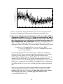
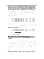
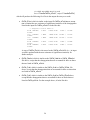
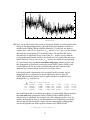
RHtestsV4
User Manual
By
Xiaolan L. Wang and Yang Feng
Climate Research Division
Atmospheric Science and Technology Directorate
Science and Technology Branch, Environment Canada
Toronto, Ontario, Canada
Published online at
http://etccdi.pacificclimate.org/software.shtml
20 July 2013
1
Table of contents
1. Introduction
2. Input data format for the RHtestsV4
3. How to use the RHtestsV4 functions
3.1 Jump start with graphical user interface (GUI)
3.2 The case “with a reference series”
3.3 The case “without a reference series”
References
Acknowledgements
2
1. Introduction
The RHtestsV4 software package is the RHtestsV3 with the addition of provision of QMadjustments that are estimated with the use of a reference series (in all cases where the
changepoint detection is done with a reference series; Vincent et al. 2012). The
RHtestsV3 software package is an extended version of the RHtestV2 package. The
extension includes: (1) provision of Quantile-Matching (QM) adjustments (Wang et al.
2010) in addition to the mean-adjustments provided in the previous versions; (2) choice
of using the whole or part of the segments before and after a shift to estimate the QMadjustments; (3) choice of the segment to which the base series is to be adjusted (referred
to as the base segment); (4) choices of the nominal level of confidence at which to
conduct the test, and (5) all functions are now available in the GUI mode.
The objective of the QM adjustments is to adjust the series so that the empirical
distributions of all segments of the de-trended base series match each other; the
adjustment value depends on the empirical frequency of the datum to be adjusted (i.e. it
varies from one datum to another in the same segment, depending on their corresponding
empirical frequencies). As a result, the shape of the distribution is often adjusted
(including, but not limited to, the adjustment to the mean), although the tests are meant to
detect mean-shifts (thus, a change in the distribution without a shift in the mean could go
undetected); and the QM adjustments could account for a seasonality of discontinuity
(e.g., it is possible that winter and summer temperatures are adjusted differently because
they belong to the lower and upper quartiles of the distribution, respectively).
Importantly, the annual cycle, lag-1 autocorrelation, and linear trend of the base series
were estimated in tandem while accounting for all identified shifts (Wang 2008a); and the
trend component estimated for the base series is preserved in the QM adjustments when
they are estimated without using a reference series . Whenever possible, QM-adjustments
should be estimated using a reference series that has homogeneous data series for a
period encompassing the shift in the base series to be adjusted.
This software package can be used to detect, and adjust for, multiple changepoints
(shifts) that could exist in a data series that may have first order autoregressive errors [but
excluding daily precipitation data series, for which the RHtests_dlyPrcp package (Wang
et al. 2010) should be used]. It is based on the penalized maximal t test (Wang et al.
2007) and the penalized maximal F test (Wang 2008b), which are embedded in a
recursive testing algorithm (Wang 2008a), with the lag-1 autocorrelation (if any) of the
time series being empirically accounted for. The time series being tested may have zerotrend or a linear trend throughout the whole period of record. The problem of uneven
distribution of false alarm rate and detection power is also greatly alleviated by using
empirical penalty functions. Therefore, the RHtestsV4 (and RHtestsV3 and RHtestV2)
has significant improvements over RHtestV0.95, which did not account for any
autocorrelation and did not resolve the problem of uneven distribution of false alarm rate
and detection power (Wang et al. 2007, Wang 2008b). A homogenous time series that is
well correlated with the base series may be used as a reference series. However, detection
of changepoints is also possible with the RHtestsV4 package when a homogenous
reference series is not available. But the results are less reliable and need intensive
3
analysis. One should not conduct data homogenization in an automatic manner
without using a reference series (i.e., without intensive manual analysis of the
statistical test results).
This simple manual is to provide a quick reference to the usage of the functions included
in the RHtestsV4 package (and also to the usage of the equivalent FORTRAN functions,
which are available by sending a request in English to [email protected]). Users
are assumed to have the general knowledge of R (how to start and end an R session and
how to call an R function).
2. Input data format for the RHtestsV4
 The RHtestsV4 functions can handle annual/monthly/daily series of Gaussian
errors (note that the RHtests_dlyPrcp package should be used for homogenization
of daily precipitation series, which are typically non-Gaussian; it is okay to apply
the RHtestsV4 functions to a log-transformed monthly/annual total
precipitation series). Each input data series should be stored in a separate file
(e.g., a file named Example.dat), in which the first three columns are the dates
(calendar year YYYY, month MM, and day DD) of observations, and the fourth
column, the observed data values (or missing value code). Note that for monthly
series DD=00, and for annual series MM=00 and DD=00. For example,
(Daily series)
…
1994 1 27
8.1
1994 1 28
5.3
1994 1 29
4.9
1994 1 30
4.9
1994 1 31
4.0
1994 2
1
3.9
1994 2
2
7.2
1994 2
3
8.7
1994 2
4
6.3
1994 2
5 -999.
1994 2
6 -999.
1994 2
7 -999.
1994 2
8 -999.
1994 2
9
9.0
1994 2 10
6.0
…

OR
(Monthly series)
…
1967
7 00 1015.70
1967
8 00 1015.95
1967
9 00 1016.10
1967 10 00 -999.99
1967 11 00 1010.71
1967 12 00 1011.58
1968
1 00 1009.37
1968
2 00 1003.07
1968
3 00 1011.94
1968
4 00 1014.74
1968
5 00 1009.59
1968
6 00 1011.77
1968
7 00 1014.35
1968
8 00 1010.87
1968
9 00 1016.45
…
The dates of input data must be consecutive and in the calendar order. Otherwise,
the program will exit with an error message containing the first date on which the
data error occurs. For example, the four rows from 5-8 February 1994 in the daily
series example above must be included in the input data file. They should not be
deleted because they are missing values. February 10, 1994 should not occur
before February 9, 1994, etc.
The above requirement applies to both the base and the reference series if used.
The base and reference series can have data for different periods (they need not be
of the same length), but only the periods common to both base and reference
series are tested/analyzed. Note that the base and reference series can have
missing values at different dates/times but they must have the same missing value
4


code. All dates/times of missing values in either the base or reference series, or in
both series, are excluded from the analysis.
There exist different ways of constructing a reference series (e.g., one may wish
to use different weights for different stations to compose a reference series or use
a single station series as a reference series). Here, for each base series, one single
reference series is assumed to have been constructed by you (the user) at your
choice. The homogeneity of the reference series can be checked by calling the
function FindU (which does not need a reference series). Significant shifts
should be adjusted before the reference series is used to check the homogeneity of
the base series.
It is recommended to test the monthly series first before testing the corresponding
daily series because daily series are much noisier and thus more difficult to test
for changepoints. The results obtained from testing monthly series can be used
subjectively to help analyze the results of testing daily series. It is also
recommended that a logarithm transform of a monthly total precipitation amount
series be done before they are used as input data series here, since the tests in this
software package assume that the data series will have Gaussian errors, and that
the RHtests_dlyPrcp package should be used for homogenization of daily
precipitation series.
3. How to use the RHtestsV4 functions
The RHtestsV4 software package provides six functions for detecting, and adjusting
for, artificial shifts in data series, with or without using a reference series.
First of all, enter source (“RHtestsV4.r”) at the R prompt (“>”) to load the RHtestsV4
functions to R.
Briefly, the steps to follow are: (see sections 3.2 and 3.3 below for the details)
1) Call function FindU (or FindU.wRef) with an appropriate list of input parameters
(see Section 3.2 or 3.3 below).
2) Go to Step 5) if you don’t have metadata. Otherwise, call FindUD (or
FindUD.wRef) with an appropriate list of input parameters (see Section 3.2 or 3.3
below).
3) Modify the resulting *_mCs.txt file (the list of changepoints identified so far,
which is in the data directory, i.e., the directory in which the data series being
tested resides), if necessary, to incorporate metadata information in the results.
(Here, the * stands for a user specified prefix for the name of the output files).
4) Call function StepSize (or StepSize.wRef) with an appropriate list of input
parameters (see Section 3.2 or 3.3 below) to assess the significance and
magnitude of the retained changepoints.
5) Analyze the latest version of the *_mCs.txt file and delete the smallest shift if it is
statistically, or subjectively determined to be, not significant. Then, call function
StepSize (or StepSize.wRef) again to re-assess the significance of the remaining
5
changepoints. Repeat this procedure (5) until each and every changepoint in the
list is determined to be significant.
Specifically, the general procedure should be:
(1) Call the FindU or FindU.wRef function, to detect all changepoints that could be
significant at the nominal level even without metadata support (these are called
Type-1 changepoints). If there is no significant changepoint identified so far, the
time series being tested can be declared to be homogeneous; and there is no need to
go further in testing this series.
(2) Go to (5) if there is no metadata available, or if one wants to detect only
those changepoints that are significant even without metadata support,
i.e., Type-1 changepoints.
Otherwise, call the FindUD or FindUD.wRef function. The resulting additional
changepoints are called Type-0 changepoints (these changepoints could be
significant only if they are supported by reliable metadata. This step is meant to
help narrow down the metadata investigation, which should focus on the periods
encompassing these Type-0 changepoints). Thus, it is good enough to apply these
functions to monthly or annual series, and it is not necessary, and would take
too long time, to apply them to daily series. Namely, when analyzing daily
series, you should apply these functions to the corresponding monthly series.
(3) Investigate the available metadata to see whether or not anything happened at or
near the identified changepoint times/dates that could have caused the shifts.
Retain only those Type-0 changepoints that are actually supported by metadata,
along with all the Type-1 changepoints as identified in (1). The date of a
changepoint may be changed to the documented date of change as obtained from
the metadata if one is confident about the cause of the change; also change the
changepoint type from 1 to 0 if a Type-1 changepoint turns out to have reliable
metadata support.
(4) Call function StepSize (or StepSize.wRef) to assess the significance and magnitude
of the remaining changepoints (listed in the latest version of the *_mCs.txt file).
(5) Analyze the latest version of the *_mCs.txt file and delete the least significant
changepoint if it is determined to be not significant at the nominal level. Then, call
function StepSize (or StepSize.wRef) to re-assess the significance of the remaining
changepoints. Repeat this procedure (5) until all the retained changepoints are
significant.
In the GUI mode (Section 3.1), the final output files reside in the output subdirectory of
the data directory (i.e., where the data series being tested resides); both the data and
output directory path are also shown in the GUI window. In the command line mode
(Section 3.2 or 3.3) user gets to specify the directory for storing the output files by
including the output directory path in the output parameter string (see Section 3.2 or 3.3).
6
3.1 Jump start with graphical user interface (GUI)
The FindU, FindUD, and StepSize functions are based on the penalized maximal F
(PMF) test (Wang 2008a and 2008b), which allows the time series being tested to have a
linear trend throughout the whole period of the data record (i.e., no shift in the trend
component; see Wang 2003), with the annual cycle, linear trend, and lag-1
autocorrelation of the base series being estimated in tandem through iterative procedures,
while accounting for all the identified mean-shifts (Wang 2008a). No reference series
will be used in any of these functions; the base series is tested in this case. Please refer to
section 3.3 below for more details about these three functions.
The FindU.wRef, FindUD.wRef, and StepSize.wRef functions are based on the penalized
maximal t (PMT) test (Wang 2008a, Wang et al. 2007), which assumes that the time
series being tested has zero-trend and Gaussian errors. A reference series is needed to run
any of *.wRef functions. The base-minus-reference series is tested to identify the
position(s) and significance of changepoint(s), but a multi-phase regression (MPR) model
with a common trend is also fitted to the anomalies (relative to the mean annual cycle) of
the base series at the end to obtain the final estimates of the magnitude of shifts (see the
Appendix in Wang 2008a for details). In the MPR fit, the annual cycle, linear trend, and
lag-1 autocorrelation are estimated in tandem through iterative procedures, while
accounting for all the identified mean-shifts (Wang 2008a). Please refer to section 3.3
below for more details about these three functions.
The QMadj_GaussDLY function is for applying the QM adjustment algorithm (Wang et
al. 2010) to daily temperature data (or daily Gaussian data in general) to adjust for a list
of significant changepoints that have been identified (e.g. from applying one or more of
the six functions described above to the corresponding monthly temperature series). This
function is not suitable for adjusting daily precipitation data series. Please call the
StepSize_dlyPrcp function in the RHtests_dlyPrcp package (also available on this
website) to adjust daily precipitation data for the identified changepoints.
In this simple graphical user interface (GUI) mode, the prefix of the input data filename
is used as the prefix for the names of the output files. For example, in case of not using a
reference series, if Example.dat is the input data filename, the output files will be named
Example_*.*; when a reference series is used, for example, Base.dat and Ref.dat are the
input base and reference series, the output files will be named Base_Ref_*.*.
Specifically, the procedure is as follows:
(1) To start the GUI session, enter StartGUI() after entering source
(“RHtestsV4.r”) at the R prompt. The following window shall appear.
7
(2) People other than the RClimDex users shall skip this procedure (2).
To convert the daily data series in the RClimDex standard format to the monthly
mean series in the RHtestsV4 standard format, click the Transform Data button,
select the file of daily data series to be converted and click the Open button. This
will produce nine files: *_tmaxMLY.txt, *_tminMLY.txt, *_prcpMLY.txt, *_tminDLY.txt,
*_tmaxDLY.txt, *_prcpDLY.txt, *_prcpMLY1mm.txt, *_LogprcpMLY.txt, and
*_LogprcpMLY1mm.txt (the * stands for the prefix of the input data filename, DLY
and MLY for daily and monthly, respectively, and MLY1mm for monthly totals
of daily Prcp ≥ 1mm).
(3) This step is not needed if data are converted using the Transform Data function.
Otherwise, click the ChangePars button to set the following parameter values: (a)
the missing value code used in the data series to be tested, e.g., “-999.0” in the
window below (note that the code entered here must be exactly the same as
used in the data; e.g., “-999.” and “-999.0” are different; one can not enter “-999.”
instead of “-999.0” when “-999.0” is used in the input data series; it will produce
erroneous results); (b) the nominal level of confidence at which to conduct the
test; (c) the base segment (to which to adjust the series); (d) the number of points
(Mq) for which the empirical probability distribution function (PDF) are to be
estimated for use in deriving the QM-adjustments; and (e) the maximum number
of years of data immediately before or after a changepoint to be used to estimate
the PDF (Ny4a = 0 for choosing the whole segment). Then, click the OK button to
accept the parameter values shown in the window.
8
(4) If you have and want to use a reference series, click the FindU.wRef button to
open a window, then click on the Change buttons one-by-one to change/select the
base and/or reference data files to be used (e.g. Example1.dat and Ref1.txt shown in
the window below; NA means the file has not been selected), and click the OK
button to execute the PMT test. This will produce the following files in the output
9
directory: Example1_Ref1_1Cs.txt, Example1_Ref1_Ustat.txt, Example1_Ref1_U.dat,
and Example1_Ref1_U.pdf (see section 3.2 for description of the content of these
files). A copy of the first file is also stored in file Example1_Ref1_mCs.txt in the
output directory, which lists all changepoints that could be significant at the
nominal level even without metadata support (i.e., Type-1 changepoints).
If you do not want to use a reference series, click the FindU button to open a
window (not shown), select the data series (say Example1.dat) to be tested and
click the Open button to execute the PMF test. This will produce the following
files in the output directory: Example1_1Cs.txt, Example1_Ustat.txt, Example1_U.dat,
and Example1_U.pdf (see section 3.3 for description of the content of these files). A
copy of the first file is also stored in file Example1_mCs.txt in the output directory,
which lists all changepoints that could be significant at the nominal level even
without metadata support (i.e., Type-1 changepoints).
An example of the *1Cs.txt file looks like this:
10 changepoints in Series … Example2.dat
1 Yes
19600200 (1.0000-1.0000) 0.950
1 Yes
19650700 (0.9999-0.9999) 0.950
1 Yes
19800300 (1.0000-1.0000) 0.950
1 Yes
19820800 (1.0000-1.0000) 0.950
1 Yes
19850200 (1.0000-1.0000) 0.950
1 Yes
19851100 (0.9999-0.9999) 0.950
1 Yes
19930200 (1.0000-1.0000) 0.950
1 Yes
19940600 (1.0000-1.0000) 0.950
1 ?
19950900 (0.9965-0.9971) 0.950
1 Yes
19970400 (1.0000-1.0000) 0.950
…
5.3553
4.1634
5.2305
4.6415
4.7195
3.8607
9.1678
5.9064
3.0340
8.2999
(
(
(
(
(
(
(
(
(
(
3.06353.09773.09053.02373.00053.04573.04692.98452.99293.0497-
3.5582)
3.6009)
3.5927)
3.5000)
3.4712)
3.5283)
3.5342)
3.4552)
3.4612)
3.5398)
Here, the first column (the1’s) is an index indicating these are Type-1
changepoints. The second column indicates whether or not the changepoint is
statistically significant for the changepoint type given in the first column; they are
“Yes” or “?” in the *_1Cs.txt file, but in other *Cs.txt files they could be the
following: (1) “Yes” (significant); (2) “No” (not significant for the changepoint
type given in the first column); (3) “?” (may or may not be significant for the type
given in the first column), and (4) “YifD” (significant if it is documented, i.e.,
supported by reliable metadata). The third column lists the changepoint dates
YYYYMMDD, e.g., 19700100 denotes January 1970. The numbers in the fourth
column (in parentheses) are the 95% confidence interval of the p-value, which is
estimated assuming the changepoint is documented. The nominal p-value
(confidence level) is given in the fifth column. The last three columns are the
values of the test statistic PFmax (or PTmax ) and the 95% confidence interval of the
PFmax (or PTmax ) percentiles that correspond to the nominal confidence level,
respectively. A copy of the file OutFile_1Cs.txt is stored in file OutFile_mCs.txt in
the output directory for possible modifications later (so that an original copy is
kept unchanged).
(5) If you know all the documented changes that could cause a mean-shift,
add these changepoints in the file Example1_Ref1_mCs.txt or Example_mCs.txt if
10
they are not already there, and go to procedure (7) below. If you do not
have metadata, or if you only want to detect Type-1 changepoints, also go
to procedure (7) below. Otherwise, click the FindUD.wRef button (or FindUD in
case of not using a reference series) to identify all Type-0 changepoints (i.e.,
changepoints that could be significant only if they are supported by metadata) for
the chosen input data series. The window below will appear for you to choose or
confirm the input files to run the FindUD.wRef (or FindUD) function. Since this
step is meant to help narrow down metadata investigation, it is good enough to
apply these functions to monthly or annual series, and it is not necessary, and
would take too long time, to apply them to daily series. Namely, when
analyzing daily series, you should apply these functions to the corresponding
monthly series.
Four files will be produced in the output directory, e.g., Example1_Ref1_pCs.txt,
Example1_Ref1_UDstat.txt, Example1_Ref1_UD.dat, and Example1_Ref1_UD.pdf by
calling the FindUD.wRef function with Example1.dat and Ref1.txt as the base and
reference series (see section 3.2 for description of the content of these files); or
Example1_pCs.txt, Example1_UDstat.txt, Example1_UD.dat, and Example1_UD.pdf by
calling the FindUD function for input series Example1.dat (see section 3.3 for
description of the content of these files). A copy of Example1_Ref1_pCs.txt (or
Example1_pCs.txt) is also stored in file Example1_Ref1_mCs.txt (or
Example1_mCs.txt) in the output directory (so that the previous version of this file,
if exists, is updated).
11
(6) Investigate metadata and delete from the Example1_Ref1_mCs.txt or
Example1_mCs.txt file in the output directory all Type-0 changepoints that are not
supported by metadata. Click the StepSize.wRef button (or StepSize in case of not
using a reference series) to re-assess the significance/magnitudes of the remaining
changepoints, which will produce the following files: Example1_Ref1_fCs.txt,
Example1_Ref1_Fstat.txt, Example1_Ref1_F.dat, Example1_Ref1_F.pdf, and an
updated Example1_Ref1_mCs.txt (or Example1_fCs.txt, Example1_Fstat.txt,
Example1_F.dat, Example1_F.pdf, and an updated Example1_mCs.txt) in the output
directory (see section 3.2 or 3.3 for description of the content of these files).
Please check the input file names to ensure they are what you want to use here.
(7) Analyze the results obtained so far to determine if the smallest shift is significant
[see (T5) in section 3.2 or (F5) in section 3.3 for the details of how to do so]. If it
is determined to be not significant, delete it from the file Example1_Ref1_mCs.txt or
Example1_mCs.txt in the output directory and click the StepSize.wRef or StepSize
button to re-assess the significance and magnitudes of the remaining
changepoints, which will update (or produce) the following files with the new
estimates: Example1_Ref1_fCs.txt, Example1_Ref1_Fstat.txt, Example1_Ref1_F.dat,
Example1_Ref1_F.pdf, and Example1_Ref1_mCs.txt (or Example1_fCs.txt,
Example1_Fstat.txt, Example1_F.dat, Example1_F.pdf, and Example1_mCs.txt) in the
output directory.
(8) Repeat the procedure (7) above, until each and every changepoint retained in the
file Example1_Ref1_mCs.txt (or Example1_mCs.txt) is determined to be significant
12
(no more deletions will be done). The following four final output files are in the
output directory:
a) Example1_Ref1_fCs.txt (or Example1_fCs.txt), which lists the changepoints
identified and their significance and statistics; b) Example1_Ref1_Fstat.txt (or
Example1_Fstat.txt), which stores the estimated mean-shift sizes and a copy of the
content in Example1_Ref1_fCs.txt (or Example1_fCs.txt); c) Example1_Ref1_F.txt (or
Example1_F.dat), which stores the mean-adjusted base series in its fifth column,
the QM-adjusted base series in its ninth column, and the original base series in its
third column; and d) Example1_Ref1_F.pdf (or Example1_F.pdf). The
Example1_Ref1_F.pdf file stores six plots: (i) the base-minus-reference series; (ii)
the base anomaly series (i.e., the base series with its mean annual cycle
subtracted, also referred to as the de-seasonalized base series) and its multi-phase
regression model fit; (iii) the base series and the estimated mean-shifts and linear
trend; (iv) the mean-adjusted base series and (v) the QM-adjusted base series
(both adjusted to the base segment), and (vi) the distribution of the QMadjustments. The Example1_F.pdf file stores all except the first plot above. Please
see sections 3.2 and 3.3 for description of the content of these output files.
(9) If you are analyzing temperature data (or Gaussian data in general) and want to
adjust the daily temperature data series for the significant changepoints that have
been identified from the corresponding monthly temperature data series with a
reference series, click the QMadj_GaussDLY.wRef button to choose the associated
daily temperature series (say Example1_DLY.dat) and its reference series (say
Ref1_DLY.dat) and the list of identified changepoints (see the window below),
and click the OK button to estimate and apply the QM adjustments with the
reference series. This will produce the following three files in the output
13
directory: (a) Example1_Ref1_DLY.dat_QMadjDLY_stat.txt, which contains the
resulting statistics; (b) Example1_Ref1_DLY.dat_QMadjDLY_data.dat, which
contains the original and the adjusted daily data in its 4th and 5th column
respectively (column 6, 7, 8 are the mean-adjusted daily series, the QM
adjustments, and the mean adjustments, respectively; columns 4 + 7 = column 5;
columns 4 + 8 = column 6); and (c) Example1_Ref1_DLY.dat_QMadjDLY_plot.pdf,
which contains the following five plots: (i) the de-seasonalized daily temperature
series and its MPR fit, (ii) the original daily temperature series and its MPR fit,
(iii) the mean-adjusted daily temperature series, (iv) the QM-adjusted daily
temperature series, and (v) the distribution of the QM adjustments for each
segment adjusted.
If you do not have a reference series, click the QMadj_GaussDLY button to choose
the associated daily temperature series (say Example1_DLY.dat) and the list of
identified changepoints, and click the OK button to estimate and apply the QM
adjustments without a reference series. This will produce the following three files
in the output directory: (a) Example1_DLY.dat_QMadjDLY_stat.txt, which contains
the resulting statistics; (b) Example1_DLY.dat_QMadjDLY_data.dat, which contains
the original and the adjusted daily data in its 4th and 5th column respectively; and
(c) Example1_DLY.dat_QMadjDLY_plot.pdf, which contains the following five plots:
(i) the de-seasonalized daily temperature series and its MPR fit, (ii) the original
daily temperature series and its MPR fit, (iii) the mean-adjusted daily temperature
series, (iv) the QM-adjusted daily temperature series, and (v) the distribution of
the QM adjustments for each segment adjusted. Extra caution should be
exercised when adjusting a data time series without using a good reference
series.
If you are analyzing precipitation data and want to adjust the daily precipitation
data series for the significant changepoints that have been identified from the
corresponding monthly precipitation totals series, call the StepSize_dlyPrcp
function in the RHtests_dlyPrcp package (also available on this website) to adjust
daily precipitation data for the identified changepoints (please refer to the Quick
Guide for RClimDex and RHtest Users, which is also available on this website).
Note that the QM adjustments could be problematic (very bad) if a discontinuity
is present in the frequency of precipitation measured (see Wang et al. 2010 for
details).
In addition to the functions with GUI above, the RHtestsV4 also provides six functions
for detecting abrupt changes (mean-shifts) in annual/monthly/daily data series without a
graphical user interface. One should click the Quit button first and then call these
functions at the R prompt (see sections 3.2 and 3.3 below for the details).
14
3.2 The case “with a reference series”
The test used in this case is the penalized maximal t test (Wang et al. 2007, Wang
2008a), which assumes that the time series being tested has zero-trend and Gaussian
errors. The base-minus-reference series is tested to identify the position(s) and
significance of changepoint(s), but a multi-phase regression (MPR) model with a
common trend is also fitted to the anomalies (relative to the mean annual cycle) of the
base series at the end to obtain the final estimates of the magnitude of shifts (see the
Appendix in Wang 2008a for details). In the MPR fit, the annual cycle, linear trend, and
lag-1 autocorrelation are estimated in tandem through iterative procedures, while
accounting for all the identified mean-shifts (Wang 2008a).
In this case, the five detailed procedures are:
(T1) Call function FindU.wRef to identify all Type-1 changepoints in the base-minusreference series by entering the following at the R prompt:
FindU.wRef(Bseries=“C:/inputdata/Bfile.csv”, MissingValueCode=“-999.0”,
p.lev=0.95, Iadj=10000, Mq=10, Ny4a=0, output=“C:/results/OutFile”,
Rseries=“C:/inputdata/Rfile.csv”)
Here, the C:/inputdata/ is the data directory path and the Bfile.csv and Rfile.csv are the
names of the files containing the base and reference series, respectively (the baseminus-reference series is tested here), which reside in the data directory; the
C:/results/ is a user specified output directory path and the OutFile is a user selected
prefix for the name of the files to store the results; and -999.0 is the missing value
code that is used in the input data Bfile.csv and Rfile.csv; p.lev is a pre-set (nominal)
level of confidence at which the test is to be conducted (choose from one of these:
0.75, 0.80, 0.90, 0.95, 0.99, and 0.9999), Iadj is an integer value corresponding to
the segment to which the series is to be adjusted (referred to as the base segment),
with Iadj=10000 corresponding to adjusting the series to the last segment; Mq is the
number of points (categories) for which the empirical probability distribution
function (PDF) are to be estimated, and Ny4a is the maximum number of years of
data immediately before or after a changepoint to be used to estimate the PDF
(Ny4a=0 for choosing the whole segment). One can set Mq to any integer between
1 and 100 inclusive, or set Mq=0 if this number is to be determined
automatically by the function (the function re-sets Mq to 1 if 0 is selected
eventually or to 100 if a larger number is selected or given). The default values
used are: p.lev=0.95, Iadj=10000, Mq=12, Ny4a=0. Note that the MissingValueCode
entered here must be exactly the same as used in the data; e.g., one can not enter “999.” instead of “-999.0” when “-999.0” is used in the input data series; otherwise it will
produce erroneous results. Also, note that character strings should be included in
double quotation marks, as shown above. After a successful call, this function
produces the following five files in the output directory:

OutFile_1Cs.txt (or OutFile_mCs.txt): The first number in the first line of this
file is the number of changepoints identified in the series being tested. If this
15
number is N c  0 , the subsequent Nc lines list the dates and statistics of these
N c changepoints. For example, it looks like this for a case of N c  10 :
1
1
1
1
1
1
1
1
1
1
10
Yes
Yes
Yes
Yes
Yes
Yes
Yes
Yes
?
Yes
changepoints in Series InFile.csv
19600200 (1.0000-1.0000) 0.950
19650700 (0.9999-0.9999) 0.950
19800300 (1.0000-1.0000) 0.950
19820800 (1.0000-1.0000) 0.950
19850200 (1.0000-1.0000) 0.950
19851100 (0.9999-0.9999) 0.950
19930200 (1.0000-1.0000) 0.950
19940600 (1.0000-1.0000) 0.950
19950900 (0.9965-0.9971) 0.950
19970400 (1.0000-1.0000) 0.950
5.3553
4.1634
5.2305
4.6415
4.7195
3.8607
9.1678
5.9064
3.0340
8.2999
(
(
(
(
(
(
(
(
(
(
3.06353.09773.09053.02373.00053.04573.04692.98452.99293.0497-
3.5582)
3.6009)
3.5927)
3.5000)
3.4712)
3.5283)
3.5342)
3.4552)
3.4612)
3.5398)
The first column (the1’s) is an index indicating these are Type-1
changepoints (also indicated by the “1Cs” in the filename). The second
column indicates whether or not the changepoint is statistically significant for
the changepoint type given in the first column; all of them are “Yes” or “?”
in the *_1Cs.txt file, but in other *Cs.txt files they could be the following: (1)
“Yes” (significant); (2) “No” (not significant for the changepoint type given
in the first column); (3) “? ” (may or may not be significant for the type given
in the first column), and (4) “YifD” (significant if it is documented, i.e.,
supported by reliable metadata). The third column lists the changepoint dates
YYYYMMDD, e.g., 19600200 denotes February 1960. The numbers in the
fourth column are the 95% confidence interval of the p-value that is
estimated assuming the changepoint is documented. The nominal p-value
(confidence level) is given in the fifth column. The last three columns are the
PTmax statistics and the 95% confidence interval of the PTmax percentiles
corresponding to the nominal confidence level. A copy of the file
OutFile_1Cs.txt is stored in file OutFile_mCs.txt for possible modifications later
(so that an original copy is kept unchanged).

OutFile_Ustat.txt: In addition to all the results stored in the OutFile_1Cs.txt file,
this output file contains the parameter estimates of the ( N c  1) -phase
regression model fit, including the sizes of the mean-shifts identified, the
linear trend and lag-1 autocorrelation of the base series.

OutFile_U.dat: In this file, the 2nd column is the dates of observation; the 3rd
column is the original base series; the 4th and 5th columns are respectively the
estimated linear trend line of the base series and the mean-adjusted base
series, for shift-sizes estimated from the base-minus-reference series; the 6th
and 7th columns are similar to the 4th and 5th columns but for shift-sizes
estimated from the de-seasonalized base series; the 8th and 9th columns are
respectively the de-seasonalized base series (i.e., the base series with its the
mean annual cycle subtracted) and its multi-phase regression model fit; the
10th column is the estimated mean annual cycle together with the linear trend
and mean-shifts; the 11th column is the QM-adjusted base series (the QM16
adjustments here are estimated using the reference series); and the 12th
column is the multi-phase regression model fit to the de-seasonalized base
series without accounting for any shifts (i.e. ignore all shifts identified).

OutFile_U.pdf: This file stores six plots: (i) the base-minus-reference series,
(ii) the base anomaly series along with its multi-phase regression model fit;
(iii) the base series along with the estimated mean-shifts and linear trend; (iv)
the mean-adjusted base series and (v) the QM-adjusted base series (both
adjusted to the base segment), and (vi) the distribution of the QMadjustments (these are estimated using the reference series). An example of
the third panel looks like this:
Monthly mean wind speeds (km/hr)
16
Base
Diff
14
12
10
8
6
4
2
0
1955
1960
1965
1970
1975
1980
1985
1990
1995
2000
Time of observation
The solid trend line represents the multi-phase regression model fit to the
base series, and the dashed line, the fit with shift-sizes estimated from the
base-minus-reference series.
If there is no significant changepoint identified so far, the time series being tested
can be declared to be homogeneous; and no need to go further in testing this series.
(T2) If you know all the documented changes that could cause a shift, add these
changepoints in the file Example_mCs.txt if they are not already there, and go
to procedure (T4) now. If there is no metadata available, or if you want to
detect only those changepoints that are significant even without metadata
support (i.e., Type-1 changepoints), also go to (T4) now. Otherwise, call
function FindUD.wRef to identify all Type-0 changepoints in the base series, in the
presence of all the Type-1 changepoints listed in file OutFile_1Cs.txt, by entering the
following at the R prompt:
FindUD.wRef(Bseries=“C:/inputdata/Bfile.csv”, MissingValueCode=“-999.0”,
p.lev=0.95, Iadj=10000, Mq=10, Ny4a=0, InCs=“C:/results/OutFile_1Cs.txt”,
output=“C:/results/OutFile”, Rseries=“C:/inputdata/Rfile.csv”)
17
Here, the OutFile_1Cs.txt file contains all the Type-1 changepoints identified by
calling FindU.wRef in (T1) above, and all the other files are the same as in (T1).
After a successful call, this function also produces five files: OutFile_pCs.txt and
OutFile_mCs.txt, OutFile_UDstat.txt, OutFile_UD.pdf, and OutFile_UD.dat. The contents of
these files are similar to the relevant files in (T1), except that the changepoints that
are modeled now are those listed in the OutFile_pCs.txt or OutFile_mCs.txt file, which
contains all the Type-1 changepoints listed in OutFile_1Cs.txt, plus all Type-0
changepoints. The OutFile_mCs.txt file is now a copy of OutFile_pCs.txt for possible
modifications later. For the example above, this file now contains 18 Type-0
changepoints (not listed here), in addition to the ten Type-1 changepoints.
Since this step is meant to help narrow down metadata investigation, it is good
enough to apply these functions to monthly or annual series, and it is not
necessary, and would take too long time, to apply them to daily series. Namely,
when analyzing daily series, you should apply these functions to the
corresponding monthly series.
(T3) As mentioned earlier, the Type-0 changepoints could be statistically significant at
the pre-set level of significance only if they are supported by reliable metadata.
Also, some of the Type-1 changepoints identified could have metadata support as
well, and the exact dates of change could be slightly different from the dates that
have been identified statistically. Thus, one should now investigate available
metadata, focusing around the dates of all the changepoints (Type-1 or Type-0)
listed in OutFile_mCs.txt. Keep only those Type-0 changepoints that are supported
by metadata, along with all Type-1 changepoints. Modify the statistically
identified dates of changepoints to the documented dates of change (obtained from
highly reliable metadata) if necessary. For the example above, only two of the 18
Type-0 changepoints are supported by metadata, and the exact dates of these shifts
are found to be January 1974 and November 1975. In this case, one should modify
the OutFile_mCs.txt file to:
12 changepoints in Series
1 Yes
19600200 (
1.00001 Yes
19650700 (
0.99980 Yes
19740200 (
0.99990 Yes
19751100 19760100 (
3.4003)
1 Yes
19800300 (
1.00001 Yes
19820800 (
1.00001 Yes
19850200 (
1.00001 Yes
19851100 (
0.99991 Yes
19930200 (
1.00001 Yes
19940600 (
1.00001 ?
19950900 (
0.99631 Yes
19970400 (
1.0000-
InFile.csv
1.0000) 0.950
0.9999) 0.950
1.0000) 0.950
1.00001.0000)
1.0000)
1.0000)
1.0000)
0.9999)
1.0000)
1.0000)
0.9970)
1.0000)
0.950
0.950
0.950
0.950
0.950
0.950
0.950
0.950
5.3553 (
2.96593.9531 (
2.97754.1114 (
2.95990.950
4.5880 (
6.1548
4.6415
4.7195
3.8607
9.1678
5.9064
3.0340
8.2999
(
(
(
(
(
(
(
(
2.94032.92832.90832.94902.95152.89232.89832.9543-
3.4415)
3.4575)
3.4299)
2.93303.4003)
3.3883)
3.3588)
3.4163)
3.4215)
3.3428)
3.3503)
3.4243)
[Please do not change the format of the first three columns, which are to be
read as input later with a format that is equivalent to format(i1, a4, i10) in
FORTRAN].
18
It could also happen that no modification to the OutFile_mCs.txt is necessary (neither
in the number nor in the dates of the changepoints; so the OutFile_pCs.txt and
OutFile_mCs.txt files are still identical); in this case the procedure (T4) below can be
skipped.
(T4) Call function StepSize.wRef to re-estimate the significance and magnitude of the
changepoints listed in OutFile_mCs.txt:
StepSize.wRef(Bseries=“C:/inputdata/Bfile.csv”, MissingValueCode=“-999.0”,
p.lev=0.95, Iadj=10000, Mq=10, Ny4a=0,
InCs=“C:/results/OutFile_mCs.txt”, output=“C:/results/OutFile”,
Rseries=“C:/inputdata/Rfile.csv”)
which will produce the following five files in the output directory as a result:

OutFile_fCs.txt (or OutFile_mCs.txt), which is similar to the input file
OutFile_mCs.txt, except that it contains the new estimates of significance and
statistics of the changepoints listed in OutFile_mCs.txt. It looks like this:
1
1
0
0
1
1
1
1
1
1
1
1
Yes
Yes
Yes
Yes
Yes
Yes
Yes
Yes
Yes
Yes
?
Yes
12 changepoints in Series InFile.csv
19600200 (
1.00001.0000) 0.950
19650700 (
0.99980.9999) 0.950
19740200 (
0.99991.0000) 0.950
19751100 (
1.00001.0000) 0.950
19800300 (
1.00001.0000) 0.950
19820800 (
1.00001.0000) 0.950
19850200 (
1.00001.0000) 0.950
19851100 (
0.99990.9999) 0.950
19930200 (
1.00001.0000) 0.950
19940600 (
1.00001.0000) 0.950
19950900 (
0.99630.9970) 0.950
19970400 (
1.00001.0000) 0.950
5.3553
3.9531
4.1114
4.5880
6.1548
4.6415
4.7195
3.8607
9.1678
5.9064
3.0340
8.2999
(
(
(
(
(
(
(
(
(
(
(
(
2.96592.97752.95992.93302.94032.92832.90832.94902.95152.89232.89832.9543-
3.4415)
3.4575)
3.4299)
3.4003)
3.4003)
3.3883)
3.3588)
3.4163)
3.4215)
3.3428)
3.3503)
3.4243)
A copy of OutFile_fCs.txt is also stored as the OutFile_mCs.txt file (its input
version is updated with the new estimates of significance/statistics) for further
analysis.

OutFile_Fstat.txt, which is similar to the OutFile_Ustat.txt or OutFile_UDstat.txt file
above, except that the changepoints that are accounted for here are those that
are listed in OutFile_mCs.txt.

OutFile_F.dat, which is similar to the OutFile_U.dat or OutFile_UD.dat file above,
except that the changepoints that are accounted for here are those that are
listed in OutFile_mCs.txt.

OutFile_F.pdf, which is similar to the OutFile_U.pdf or OutFile_UD.pdf above,
except that the changepoints that are accounted for here are those that are
listed in OutFile_mCs.txt.
19
(T5) Now, one needs to analyze the results, to determine whether or not the smallest
shift among all the shifts/changepoints is still significant now (the magnitudes of
shifts are included in the OutFile_Fstat.txt or OutFile_Ustat.txt file). To this end, one
needs to compare the p-value (if it is Type-0) or the PTmax statistic (if it is Type-1) of
the smallest shift with the corresponding 95% uncertainty range. This smallest shift
can be determined to be significant if its p-value or PTmax statistic is larger than the
corresponding upper bound, and to be not significant if it is smaller than the lower
bound. However, if the p-value or the PTmax statistic lies within the corresponding
95% uncertainty range, one has to determine subjectively whether or not to take
this changepoint as significant (viewing the plot in OutFile_F.pdf or OutFile_U.pdf
could help here); this is due to the uncertainty inherent in the estimate of the
unknown lag-1 autocorrelation of the series (see Wang 2008a).
If the smallest shift is determined to be not significant, delete it from file
OutFile_mCs.txt and call function StepSize.wRef again with the new modified list of
changepoints. For the example above, the changepoint in September 1995 was
determined to be not significant, because has no metadata support and it may or may
not be a significant Type-1 changepoint (since its PTmax statistic lies within the 95%
uncertainty range of the 95th percentile). We delete it from the OutFile_mCs.txt file
and call function StepSize.wRef again, which will produce this updated
OutFile_mCs.txt file:
1
1
0
0
1
1
1
1
1
1
1
11 changepoints in Series InFile.csv
Yes
19600200 (
1.00001.0000)
Yes
19650700 (
0.99980.9999)
Yes
19740200 (
0.99991.0000)
Yes
19751100 (
1.00001.0000)
Yes
19800300 (
1.00001.0000)
Yes
19820800 (
1.00001.0000)
Yes
19850200 (
1.00001.0000)
Yes
19851100 (
0.99990.9999)
Yes
19930200 (
1.00001.0000)
Yes
19940600 (
0.99991.0000)
Yes
19970400 (
1.00001.0000)
0.950
0.950
0.950
0.950
0.950
0.950
0.950
0.950
0.950
0.950
0.950
5.3553
3.9531
4.1114
4.5880
6.1548
4.6415
4.7195
3.8607
9.1678
4.3806
12.6841
(
(
(
(
(
(
(
(
(
(
(
3.00203.01362.99602.97032.97642.96442.94442.98632.98762.95642.9964-
3.4871)
3.5017)
3.4771)
3.4445)
3.4476)
3.4325)
3.4025)
3.4605)
3.4661)
3.4245)
3.4776)
One should repeat this re-assessment procedure, i.e. repeat calling function
StepSize.wRef, until each and every changepoint listed in OutFile_fCs.txt or
OutFile_mCs.txt is determined to be significant. For the example above, all the 11
changepoints turn out to be significant Type-1 changepoints (they are significant
even without metadata support); the final fit looks like this:
20
Monthly mean wind speeds (km/hr)
16
Base
Diff
14
12
10
8
6
4
2
0
1955
1960
1965
1970
1975
1980
1985
Time of observation
1990
1995
2000
Note that two sets of mean-shift size estimates (mean-adjustments) are provided
here: one estimated from the base series, another from the difference series. Users
have the options and are responsible to determine what adjustments to make.
Caution shall be exercised when there is a significant discrepancy between the two
sets of estimates, which could arise from inhomogeneity of the reference series, or
from the existence of some other changepoints that are not identified (the chance for
such failure equals the pre-set level α). In case of reference series inhomogeneity, the
estimates from the difference series should not be used (otherwise it would introduce
one or more new changepoints to the base series); the adjustments estimated from
the base series are better in this case and should be used. When all significant
changepoints are accounted for and the reference series is homogeneous, the two sets
of estimates should be similar, as shown in the plot above.
3.3 The case “without a reference series”
Caution: The results of changepoint detection without the use of a reference series
are less reliable and need intensive analysis. One should not conduct data
homogenization in an automatic manner without using a reference series (i.e., without
intensive manual analysis of the statistical test results). Extra caution should be exercised
when adjusting a data time series without using a good reference series.
The test used in this section is the penalized maximal F test (Wang 2008a and 2008b),
which allows the time series being tested to have a linear trend throughout the whole
period of data record (i.e., no shift in the trend component; see Wang 2003), with the
annual cycle, linear trend, and lag-1 autocorrelation of the base series being estimated in
tandem through iterative procedures, while accounting for all the identified mean-shifts
(Wang 2008a). This is basically the same as the case described in section 3.1 above,
except that there is no graphical user interface. The time series being tested here can be a
21
base series (the true without a reference series case) or a base-minus-reference series (in a
single ready-to-use series). The latter is recommended only if a difference between the
trends of the base and the reference series is suspected; in this case, the parameter
estimates for the base series need to be obtained by extra call(s) to the StepSize function
with the base series and the changepoints that are identified from the base-minusreference series [see procedure (F5) in this section].
In this case, the five detailed procedures are:
(F1) Call function FindU to identify all Type-1 changepoints in the InSeries by entering
the following at the R prompt:
FindU(InSeries=“C:/inputdata/InFile.csv”, MissingValueCode=“-999.0”,
p.lev=0.95, Iadj=10000, Mq=10, Ny4a=0, output=“C:/results/OutFile”)
Here, the C:/inputdata/ is the data directory path and the InFile.csv is the name of the
file containing the data series to be tested; while C:/results/ is a user specified output
directory path and the OutFile is a user selected prefix for the name of the files to
store the results; -999.0 is the missing value code that is used in the input data file
InFile.csv; p.lev is a pre-set (nominal) level of confidence at which the test is to be
conducted (choose from one of these: 0.75, 0.80, 0.90, 0.95, 0.99, and 0.9999), Iadj
is an integer value corresponding to the segment to which the series is to be
adjusted (referred to as the base segment), with Iadj=10000 corresponding to
adjusting the series to the last segment; Mq is the number of points (categories)
for which the empirical probability distribution function (PDF) are to be
estimated, and Ny4a is the maximum number of years of data immediately
before or after a changepoint to be used to estimate the PDF (Ny4a=0 for
choosing the whole segment). One can set Mq to any integer between 1 and 100
inclusive, or set Mq=0 if this number is to be determined automatically by the
function (the function re-sets Mq to 1 if 0 is selected eventually or to 100 if a
larger number is selected or given). The default values used are: p.lev=0.95,
Iadj=10000, Mq=12, Ny4a=0. Note that the MissingValueCode entered here must be
exactly the same as used in the data; e.g., one cannot enter “-999.” instead of “-999.0”
when “-999.0” is used in the input data series; otherwise it will produce erroneous
results. Also, note that character strings should be included in double quotation
marks, as shown above. After a successful call, this function produces the following
five files in the output directory:

OutFile_1Cs.txt (and OutFile_mCs.txt): The first number in the first line of this
file is the number of changepoints identified in the series being tested. If this
number is N c  0 , the subsequent Nc lines list the dates and statistics of these Nc
changepoints. For example, it looks like this for a case of N c  3 :
3 changepoints in Series InFile.csv
1 Yes
19700100 (1.0000-1.0000) 0.950
1 Yes
19740200 (1.0000-1.0000) 0.950
1 Yes
19760600 (1.0000-1.0000) 0.950
22
49.2060 (
23.3712 (
21.4244 (
14.285713.275814.4950-
19.2003)
17.7289)
19.5295)
The first column (the1’s) is an index indicating these are Type-1 changepoints
(also indicated by the “1Cs” in the filename). The second column indicates
whether or not the changepoint is statistically significant for the changepoint
type given in the first column; all of them are “Yes” in this *_1Cs.txt file, but
in other *Cs.txt files they could be the following: (1) “Yes” (significant); (2)
“No” (not significant for the changepoint type given in the first column); (3) “?
” (may or may not be significant for the type given in the first column), and (4)
“YifD” (significant if it is documented, i.e., supported by reliable metadata).
The third column lists the changepoint dates YYYYMMDD, e.g., 19700100
denotes January 1970. The numbers in the fourth column (in parentheses) are
the 95% confidence interval of the p-value, which is estimated assuming the
changepoint is documented (thus this value is very high for a significant Type1 changepoint). The nominal p-value (confidence level) is given in the fifth
column. The last three columns are the PFmax statistics and the 95% confidence
interval of the PFmax percentiles that correspond to the nominal confidence
level, respectively. A copy of the file OutFile_1Cs.txt is stored in file
OutFile_mCs.txt in the output directory for possible modifications later (so that
an original copy is kept unchanged).

OutFile_Ustat.txt: In addition to all the results stored in the OutFile_1Cs.txt file,
this output file contains the parameter estimates of the ( N c  1) -phase regression
model fit, including the sizes of the mean-shifts identified, the linear trend and
lag-1 autocorrelation of the series being tested.

OutFile_U.dat: This file contains the dates of observation (2nd column), the
original base series (3rd column), the estimated linear trend and mean-shifts of
the base series (4th column), the mean-adjusted base series (5th column), the
base anomaly series (i.e., the base series with its the mean annual cycle
subtracted) and its multi-phase regression model fit (6th and 7th columns,
respectively), the estimated mean annual cycle together with the linear trend
and mean-shifts (8th column), the QM-adjusted base series (9th column), and
the multi-phase regression model fit to the de-seasonalized base series without
accounting for any shifts (i.e. ignore all shifts identified; 10th column).

OutFile_U.pdf: This file stores five plots: (i) the base anomaly series (i.e.,
anomalies relative to the mean annual cycle of the base series) along with its
multi-phase regression model fit; (ii) the base series along with the estimated
mean-shifts and linear trend; (iii) the mean-adjusted base series and (iv) the
QM-adjusted base series (both adjusted to the base segment), and (v) the
distribution of the QM-adjustments. An example of the second panel looks like
this:
23
18
16
Wind speed (km/hr)
14
12
10
8
6
4
1955
1960
1965
1970
1975
1980
1985
Time of observation
1990
1995
2000
2005
If there is no significant changepoint identified, the time series being tested can be
declared to be homogeneous; and no need to go further in testing this series.
(F2) If you know all the documented changes that could cause a shift, add these
changepoints in the file Example_mCs.txt if they are not already there, and go
to (F4) now. If there is no metadata available, or if you want to detect only
those changepoints that are significant even without metadata support (i.e.,
Type-1 changepoints), also go to (F4) now. Otherwise, call function FindUD to
identify all Type-0 changepoints in the series, in the presence of all the Type-1
changepoints listed in file OutFile_1Cs.txt, by entering the following at the R prompt:
FindUD(InSeries=“C:/inputdata/InFile.csv”, MissingValueCode=“-999.0”,
p.lev=0.95, Iadj=10000, Mq=10, Ny4a=0, InCs=“C:/results/OutFile_1Cs.txt”,
output=“C:/results/OutFile”)
Here, the OutFile_1Cs.txt file contains all the Type-1 changepoints identified by
calling FindU in (F1) above, and all the other files are the same as in (F1). Here, a
successful call also produces five files: OutFile_pCs.txt and OutFile_mCs.txt,
OutFile_UDstat.txt, OutFile_UD.pdf, and OutFile_UD.dat. The contents of these files are
similar to the relevant files in (F1), except that the changepoints that are now
modeled are those listed in the OutFile_pCs.txt or OutFile_mCs.txt file, which contains
all the Type-1 changepoints listed in OutFile_1Cs.txt, plus all Type-0 changepoints.
The OutFile_mCs.txt file is now a copy of OutFile_pCs.txt for possible modifications
later.
Since this step is meant to help narrow down metadata investigation, it is good
enough to apply these functions to monthly or annual series, and it is not
necessary, and would take too long time, to apply them to daily series. Namely,
when analyzing daily series, you should apply these functions to the
corresponding monthly series.
24
(F3) As mentioned earlier, the Type-0 changepoints could be statistically significant at
the pre-set level of significance only if they are supported by reliable metadata.
Also, some of the Type-1 changepoints identified could have metadata support as
well, and the exact dates of change could be slightly different from the dates that
have been identified statistically. Thus, one should now investigate available
metadata, focusing around the dates of all the changepoints (Type-1 or Type-0)
listed in the OutFile_mCs.txt file. Keep only those Type-0 changepoints that are
supported by metadata, along with all Type-1 changepoints. Modify the
statistically identified dates of changepoints to the documented dates of change
(obtained from highly reliable metadata) if necessary. For example, the original
OutFile_mCs.txt is as follows:
0
1
1
1
0
5 changepoints in Series InFile.csv
YifD 19661100 (0.9585-0.9631) 0.950
Yes
19700100 (1.0000-1.0000) 0.950
Yes
19740200 (1.0000-1.0000) 0.950
No
19760600 (0.9947-0.9949) 0.950
YifD 19800500 (0.9611-0.9725) 0.950
4.5890
49.2842
23.4044
8.2628
5.5643
(
(
(
(
(
13.933413.224913.103013.073114.2667-
18.7098)
17.6775)
17.4929)
17.4490)
19.2069)
If it is determined after metadata investigation that there are documented causes for
three shifts, and that the exact dates of these shifts are November 1966, July 1976,
and March 1980, one should modify the OutFile_mCs.txt file to (the modified
numbers are shown in bold):
5 changepoints in Series InFile.csv
0 YifD 19661100 (0.9585-0.9631) 0.950
4.5890 (
13.933418.7098)
1 Yes
19700100 (1.0000-1.0000) 0.950
49.2842 (
13.224917.6775)
1 Yes
19740200 (1.0000-1.0000) 0.950
23.4044 (
13.103017.4929)
0
19760700 19760600 (0.9947-0.9949) 0.950
8.2628 (
13.073117.4490)
0 YifD 19800300 19800500 (0.9611-0.9725) 0.950
5.5643 (
14.266719.2069)
[Please do not change the format of the first three columns, which are to be
read as input later with a format that is equivalent to format(i1, a4, i10) in
FORTRAN]
Note that the above example is a case in which all the Type-0 changepoints have
metadata support. However, it could happen that metadata support is not found for
some of the Type-0 changepoints identified; in this case, all the un-supported Type-0
changepoints should be deleted from the list (see the example in section 3.3 below).
It could also happen that no modification to the OutFile_mCs.txt is necessary (neither
in the number nor in the dates of the changepoints; so the OutFile_pCs.txt and
OutFile_mCs.txt files are still identical); in this case the procedure (F4) below can be
skipped.
(F4) Call function StepSize to re-estimate the significance and magnitude of the
changepoints listed in OutFile_mCs.txt, e.g., enter at the R prompt the following:
StepSize(InSeries=“C:/inputdata/InFile.csv”, MissingValueCode=“-999.0”,
25
p.lev=0.95, Iadj=10000, Mq=10, Ny4a=0,
InCs=“C:/results/OutFile_mCs.txt”, output=“C:/results/OutFile”)
which will produce the following five files in the output directory as a result:

OutFile_fCs.txt, which is similar to the input file OutFile_mCs.txt above, except
that it contains the new estimates of significance/statistics of the changepoints
listed in the input file OutFile_mCs.txt. It looks like this:
5 changepoints in Series InFile.csv
0 YifD 19661100 (
0.95930.9642) 0.950
18.7232)
1 Yes
19700100 (
1.00001.0000) 0.950
17.6898)
1 Yes
19740200 (
1.00001.0000) 0.950
17.5270)
0 YifD 19760700 (
0.98980.9915) 0.950
17.4171)
0 YifD 19800300 (
0.95860.9648) 0.950
19.2186)
4.6639 (
13.9432-
49.2263 (
13.2341-
24.9972 (
13.1271-
7.4609 (
13.0522-
4.8066 (
14.2757-
A copy of OutFile_fCs.txt is also stored as the OutFile_mCs.txt file (i.e., its input
version is updated with the new estimates of significance/statistics) for
further analysis.

OutFile_Fstat.txt, which is similar to the OutFile_Ustat.txt or OutFile_UDstat.txt
file above, except that the changepoints that are accounted for here are those
that are listed in OutFile_mCs.txt.

OutFile_F.dat, which is similar to the OutFile_U.dat or OutFile_UD.dat file
above, except that the changepoints that are accounted for here are those that
are listed in OutFile_mCs.txt.

OutFile_F.pdf, which is similar to the OutFile_U.pdf or OutFile_UD.pdf above,
except that the changepoints that are accounted for here are those that are
listed in OutFile_mCs.txt. For the example above, it looks like this:
26
18
16
Wind speed (km/hr)
14
12
10
8
6
4
1955
1960
1965
1970
1975
1980
1985
Time of observation
1990
1995
2000
2005
(F5) Now, one needs to analyze the results, to determine whether or not the smallest shift
among all the shifts/changepoints is still significant (the magnitudes of shifts are
included in the OutFile_Fstat.txt or OutFile_Ustat.txt file). To this end, one needs to
compare the p-value (if it is Type-0) or PFmax statistic (if it is Type-1) of the smallest
shift with the corresponding 95% uncertainty range. This smallest shift can be
determined to be significant if its p-value or the PFmax statistic is larger than the
corresponding upper bound, and to be not significant if it is smaller than the lower
bound. However, if the p-value or the PFmax statistic lies within the corresponding
95% uncertainty range, one has to determine subjectively whether or not to take
this changepoint as significant (viewing the plot in OutFile_F.pdf or OutFile_U.pdf
could help here); this is due to the uncertainty inherent in the estimate of the
unknown lag-1 autocorrelation of the series (see Wang 2008a).
If the smallest shift is determined to be not significant (for example, the last
changepoint above is determined to be not significant), delete it from file
OutFile_mCs.txt and call function StepSize again with the new modified list of
changepoints, e.g., with this list:
0
1
1
0
4 changepoints in Series InFile.csv
YifD 19661100 (
0.96980.9721) 0.950
Yes
19700100 (
1.00001.0000) 0.950
Yes
19740200 (
1.00001.0000) 0.950
Yes
19760700 (
1.00001.0000) 0.950
5.0424
48.8569
24.5542
20.7045
(
(
(
(
13.983213.271513.164114.3520-
18.7773)
17.7404)
17.5771)
19.3331)
One should repeat this re-assessment procedure (i.e. repeat calling function StepSize)
until each and every changepoint listed in OutFile_fCs.txt or OutFile_mCs.txt is
determined to be significant. For example, if the first changepoint above (now the
smallest shift among the four) is also determined to be not significant, one should
delete it and call function StepSize again with the remaining three changepoints,
which would produce the following new estimates in the OutFile_fCs.txt:
3
changepoints in Series InFile.csv
27
1 Yes
1 Yes
0 Yes
19700100 (
19740200 (
19760700 (
1.00001.00001.0000-
1.0000) 0.950
1.0000) 0.950
1.0000) 0.950
49.1132 (
25.0495 (
21.0748 (
14.277813.283814.4869-
19.1894)
17.7413)
19.5183)
Here, all these three changepoints are significant even without metadata support,
because each of the corresponding PFmax statistics (column 5 above) is larger than
the upper bound of its percentile that corresponds to the nominal level (the last
number in each line). Thus, the results obtained from the last call to function
StepSize are the final results for the series being tested.
Note that if the series being tested above is a base-minus-reference series (not the
base series itself), one needs to repeat calling function StepSize again, with the base
series as the InFile.csv and the changepoints listed in the latest version of
OutFile_fCs.txt or OutFile_mCs.txt, to obtain the final parameter estimates for the base
series.
References
Vincent, L. A., X. L. Wang, E. J. Milewska, H. Wan, Y. Feng, and V. Swail,
2012: A Second Generation of Homogenized Canadian Monthly Surface
Air Temperature for Climate Trend Analysis, JGR-Atmospheres, 117,
D18110, doi:10.1029/2012JD017859.
Wang, X. L., H. Chen, Y. Wu, Y. Feng, and Q. Pu, 2010: New techniques for
detection and adjustment of shifts in daily precipitation data series. J.
Appl. Meteor. Climatol. 49 (No. 12), 2416-2436. DOI:
10.1175/2010JAMC2376.1
Wang, X. L., 2008a: Accounting for autocorrelation in detecting mean-shifts in
climate data series using the penalized maximal t or F test. J. Appl.
Meteor. Climatol., 47, 2423-2444.
Wang, X. L., 2008b: Penalized maximal F-test for detecting undocumented meanshifts without trend-change. J. Atmos. Oceanic Tech., 25 (No. 3), 368-384.
DOI:10.1175/2007/JTECHA982.1.
Wang, X. L., Q. H. Wen, and Y. Wu, 2007: Penalized maximal t test for detecting
undocumented mean change in climate data series. J. Appl. Meteor.
Climatol., 46 (No. 6), 916-931. DOI:10.1175/JAM2504.1
Wang, X. L., 2003: Comments on “Detection of Undocumented Changepoints: A
Revision of the Two-Phase Regression Model”. J. Climate, 16, 33833385.
Acknowledgements
The authors wish to thank Xuebin Zhang and Enric Aguilar for their helpful comments on
an earlier version of this manual, and to Hui Wan and Lucie Vincent and Enric Aguilar
for their help in testing use of the software package. Jeff Robel of the National Climatic
Data Center of NOAA (USA) is acknowledged for his helpful review and editing of the
previous version of the manual (i.e. the RHtestV2 User Guide).
28
29