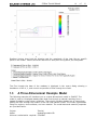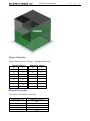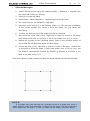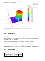
Download 1 SVHeat Tutorial Manual

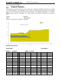
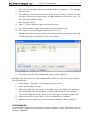
2D / 3D Geothermal Modeling Software
Tutorial Manual
Written by:
Robert Thode, B.Sc.G.E., P.Eng.
Edited by:
Murray Fredlund, Ph.D., P.Eng.
SoilVision Systems Ltd.
Saskatoon, Saskatchewan, Canada
Software License
The software described in this manual is furnished under a license agreement. The software may be used or
copied only in accordance with the terms of the agreement.
Software Support
Support for the software is furnished under the terms of a support agreement.
Copyright
Information contained within this Tutorial Manual is copyrighted and all rights are reserved by SoilVision
Systems Ltd. The SVHEAT software is a proprietary product and trade secret of SoilVision Systems.
The Tutorial Manual may be reproduced or copied in whole or in part by the software licensee for use
with running the software. The Tutorial Manual may not be reproduced or copied in any form or by any
means for the purpose of selling the copies.
Disclaimer of Warranty
SoilVision Systems Ltd. reserves the right to make periodic modifications of this product without obligation
to notify any person of such revision. SoilVision does not guarantee, warrant, or make any representation
regarding the use of, or the results of, the programs in terms of correctness, accuracy, reliability, currentness,
or otherwise; the user is expected to make the final evaluation in the context of his (her) own problems.
Trademarks
Windows™ is a registered trademark of Microsoft Corporation.
SoilVision® is a registered trademark of SoilVision Systems Ltd.
SVOFFICE ™ is a trademark of SoilVision Systems Ltd.
SVFLUX ™ is a trademark of SoilVision Systems Ltd.
CHEMFLUX ™ is a trademark of SoilVision Systems Ltd.
SVAIRFLOW ™ is a trademark of SoilVision Systems Ltd.
SVSOLID ™ is a trademark of SoilVision Systems Ltd.
SVHEAT ™ is a trademark of SoilVision Systems Ltd.
SVDYNAMIC ™ is a trademark of SoilVision Systems Ltd.
ACUMESH ™ is a trademark of SoilVision Systems Ltd.
FlexPDE® is a registered trademark of PDE Solutions Inc.
Copyright © 2008
by
SoilVision Systems Ltd.
Saskatoon, Saskatchewan, Canada
ALL RIGHTS RESERVED
Printed in Canada
Table of Contents
...................................................................................................................................
1 SVHeat Tutorial Manual
...................................................................................................................................
1.1 Introduction
...................................................................................................................................
1.2 Heated Pipeline
1.2.1 Model Setup
...................................................................................................................................
1.2.2 Results & Discussion
...................................................................................................................................
...................................................................................................................................
1.3 A Three-Dimensional Example Model
1.3.1 Model Setup
...................................................................................................................................
1.3.2 Results & Discussion
...................................................................................................................................
...................................................................................................................................
1.4 References
...................................................................................................................................
1.5 Appendix A
3
of
32
4
5
6
7
16
18
20
30
31
31
SVHeat Tutorial Manual
1
4
of
32
SVHeat Tutorial Manual
Tutorial Manual
Written by:
Robert Thode, B.Sc.G.E.
Edited by:
Murray Fredlund, Ph.D.
SoilVision Systems Ltd.
Saskatoon, Saskatchewan, Canada
Software License
The software described in this manual is furnished under a license agreement. The software
may be used or copied only in accordance with the terms of the agreement.
SVHeat Tutorial Manual
5
of
32
Software Support
Support for the software is furnished under the terms of a support agreement.
Copyright
Information contained within this Tutorial Manual is copyrighted and all rights are reserved
by SoilVision Systems Ltd. The SVHEAT software is a proprietary product and trade secret
of SoilVision Systems. The Tutorial Manual may be reproduced or copied in whole or in part
by the software licensee for use with running the software. The Tutorial Manual may not be
reproduced or copied in any form or by any means for the purpose of selling the copies.
Disclaimer of Warranty
SoilVision Systems Ltd. reserves the right to make periodic modifications of this product
without obligation to notify any person of such revision. SoilVision does not guarantee,
warrant, or make any representation regarding the use of, or the results of, the programs in
terms of correctness, accuracy, reliability, currentness, or otherwise; the user is expected to
make the final evaluation in the context of his (her) own models.
Trademarks
WindowsÔ is a registered trademark of Microsoft Corporation.
SoilVisionÒ is a registered trademark of SoilVision Systems Ltd.
SVOFFICE Ô is a trademark of SoilVision Systems, Ltd.
CHEMFLUX Ô is a trademark of SoilVision Systems Ltd.
SVFLUX Ô is a trademark of SoilVision Systems Ltd.
SVHEAT Ô is a trademark of SoilVision Systems Ltd.
SVAIRFLOW Ô is a trademark of SoilVision Systems Ltd.
SVSOLID Ô is a trademark of SoilVision Systems Ltd.
SVDYNAMIC Ô is a trademark of SoilVision Systems Ltd.
ACUMESH Ô is a trademark of SoilVision Systems Ltd.
FlexPDEÒ is a registered trademark of PDE Solutions Inc.
Copyright Ó 2008
by
SoilVision Systems Ltd.
Saskatoon, Saskatchewan, Canada
ALL RIGHTS RESERVED
Printed in Canada
1.1
Introduction
The Tutorial Manual serves a special role in guiding the first time users of the SVHEAT
software through a typical example problem. The example is "typical" in the sense that it is
not too rigorous on one hand and not too simple on the other hand.
The Tutorial Manual serves as a guide by: assisting the user with the input of data necessary
to solve the boundary value problem, ii.) explaining the relevance of the solution from an
engineering standpoint, and iii.) assisting with the visualization of the computer output. An
attempt has been made to ascertain and respond to questions most likely to be asked by
6
SVHeat Tutorial Manual
of
32
first time users of SVHEAT.
1.2
Heated Pipeline
The following example introduces some of the basic features of SVHEAT and sets up a model
of a buried pipeline. The purpose of this model is to determine the effects of the heated
pipeline on the frozen ground and the nearby roadway. This steady-state model is composed
of two regions and two materials. The model data and material properties are provided
below.
Project:
Highway
Model:
PipLineTut2D
Minimum authorization required: STUDENT
Model Description
Slope Region
Seam Region
Shape 1 - polygon
X
0
100
100
90
80
50
40
35
33
23
21
0
0
0
Y
0
0
30
30
28
28
20
20
22
22
20
20
15
10
Shape 2 -Circle
Center:
X
50
Radius:
2
Y
18
X
0
55
40
0
Y
10
10
15
15
SVHeat Tutorial Manual
7
of
32
Material Properties
The only soil properties required to solve this problem are those related to thermal
conductivity since a steady-state analysis is being performed.
Material 1 - Slope Region:
Temperature (oC)
-10
-1
-0.1
0
0.1
1
10
Conductivity (J/hr-m- oC)
1.58E+05
1.57E+05
1.56E+05
1.43E+05
1.28E+05
1.29E+05
1.30E+05
Material 2 - Seam Region:
Temperature (oC)
-10
-1
-0.1
0
0.1
1
10
1.2.1
Thermal Conductivity curve laboratory data:
Thermal Conductivity curve laboratory data:
Conductivity (J/hr-m- oC)
2.00E+05
1.90E+05
1.80E+05
1.50E+05
1.30E+05
1.25E+05
1.20E+05
Model Setup
The following steps are required in order to set up and solve the model described in the
preceding section. The steps fall under the general categories of:
a.
Create model
b.
Enter geometry
c.
Specify boundary conditions
d.
Apply material properties
e.
Specify model output
f.
Run model
g.
Visualize results
a. Create Model
The following steps are required to create the model:
1.
Open the SVOFFICE Manager dialog.
2.
Create a new project called Tutorial by pressing the New button next to the list
of projects.
SVHeat Tutorial Manual
3.
8
of
32
Create a new model called Heated_Pipeline by pressing the New button next to
the list of models. The new model will be automatically added under the recently
created UserTutorial project. Use the settings shown below when creating a new
model.
4.
Select the following:
·
SVFlux for Application
·
2D for System,
·
Steady-State for Type,
·
Metric for Units, and
·
Seconds (s) for Time Units.
Click on OK.
Before entering any model geometry it is best to set the World Coordinate System to ensure
that the model will fit into the drawing space.
1.
Access the World Coordinate System tab by selecting the World Coordinate
System tab on the Create New Model dialog.
2.
Enter the World Coordinates System coordinates shown below into the dialog.
x-minimum = -5
y-minimum = -5
x-maximum = 105
y-maximum = 105
3.
Click OK to close the dialog.
The workspace grid spacing needs to be set to aid in defining region shapes. The Seam
Region in this example consists of a filter type material. The filter material of the model has
coordinates of a precision of 0.5m. In order to draw any aspect of the geometry with this
precision using the mouse, the grid spacing must be set to a maximum value of 0.5.
1.
Select View > Options from the menu to access the Grid Spacing.
2.
Enter 0.5 for both the horizontal and vertical spacing.
3.
Click OK to close the dialog.
b. Enter Geometry
A region is the basic building block for a model. A region represents both a physical portion
of material being modeled and a visualization area in the SVHEAT CAD workspace. A region
will have a set of geometric shapes (e.g., polygons, circles, etc.) that define its material
boundaries. Other modeling objects include features, such as flux sections, text, and line art.
These features can be defined on any given region.
The present model is divided into two regions; namely the Slope region and the Seam
region. Use the following steps to add the necessary regions:
1.
Open the regions dialog by selecting Model > Geometry > Regions from the
menu.
SVHeat Tutorial Manual
2.
9
of
32
Change the first region name from Region 1 to Slope. To do this, highlight the
name and type the new name (Slope).
3.
Press the New button to add a second region.
4.
Change the name of the second region to Seam.
5.
Click OK to close the dialog.
The shapes that define each material region are now created. Note that when drawing a
geometric shape, information will be added to the region that is current in the Region
Selector. The Region Selector is found at the top of the workspace and appears in the
following image:
·
Define the Slope Region – Shape 1
Shape 1 refers to the entire region consisting of material 1.
1.
Select Slope as the region by going to Model > Geometry > Regions and clicking
on 'Slope'.
2.
Select Draw > Model Geometry > Region Polygon from the menu.
3.
The cursor will now be changed to cross hairs.
4.
Move the cursor near (0,0) in the drawing space. You can view the coordinates
of the current position of the mouse in the status bar just below the drawing
space.
5.
To select the point as part of the shape, left click on the point.
6.
Now move the cursor near (100,0). Left click on the point. A line is now drawn
from (0,0) to (100,0).
7.
Repeat this process for the remaining points as provided at the beginning of this
tutorial. This will define the geometry of the Slope Region.
8.
For the last point (0,10), double-click on the point to finish the shape. A line is
now drawn from (0,15) to (0,10) and the shape is automatically finished.
SVHEAT will draw a line from (0,10) back to the starting point, (0,0).
NOTE:
At times it may be somewhat tricky to snap onto a grid point that is near a line
defined for a region. Turn the object snap off by clicking on “OSNAP” in the status bar
to alleviate this problem.
·
Define the Slope Region – Shape 2
Shape 2 refers to the geometry of the heated pipeline.
9.
Ensure the “Slope” region is current in the region selector.
10. Select Draw > Model Geometry > Region Circle from the menu.
11. The cursor will now be changed to cross hairs.
10
SVHeat Tutorial Manual
12. Move the
cursor near (50,18) in the
drawing
of
32
space. You can view the
coordinates of the current position of the mouse in the status bar just below the
drawing space.
13. To select the point as the circle center left click on the desired point.
14. Drag the cursor out to a radius of 2.
15. Let go of the mouse button to finish the circle.
16. To ensure that the radius is set to 2, open the double-click on the circle shape to
open the Region Properties dialog.
17. Enter a radius of 2 if necessary.
18. Click OK to close the Region Properties dialog.
If the slope geometry been entered correctly the shape should look as follows:
NOTE:
If a mistake was made entering the coordinate points for a shape. Select a shape
with the mouse and select Edit > Delete from the menu. This will remove the entire
shape from the region. To edit the shape use the Region Properties dialog.
·
Define the Seam Region
The Seam Region corresponds to material 2 in the layout of the example.
19. Ensure that “Seam” is current in the region selector.
20. Select Draw > Model Geometry > Region Polygon from the menu.
21. The cursor will now be changed to cross hairs.
22. Move the cursor near (0,10) in the drawing space. You can view the coordinates
of the current position of the mouse in the status bar just below the drawing
space.
23. To select the point as part of the shape left click on the point.
24. Now move the cursor near (55,10). Left click on the point. A line is now drawn
from (0,10) to (55,10).
25. Now move the cursor near (40,15). Left click on the point. A line is now drawn
from (55,10) to (40,15).
26. For the last point (0,15), right click to snap the cursor to the point. Double-click
on the point to finish the shape. A line is now drawn from (40,15) to 0,15) and
the shape of the seam is automatically finished. SVHEAT will draw a line from
SVHeat Tutorial Manual
11
(0,15) back to the start point, (0,10).
The diagram will appear as shown at the beginning of this tutorial after all the region
geometries have been entered.
of
32
12
SVHeat Tutorial Manual
of
32
c. Specify Boundary Conditions
Boundary conditions must be applied to the points associated with each region. Once a
boundary condition is applied to a boundary point this defines the starting point for that
particular boundary condition. The boundary condition will then extend over subsequent line
segments around the edge of the region in the direction in which the region shape was
originally entered. Boundary conditions remain in effect around a shape until they are redefined. The user may not define two different boundary conditions to the same line
segment.
More information on boundary conditions can be found in Menu System > Model Menu >
Boundary Conditions > 2D Boundary Conditions in your User's Manual.
Now that all of the regions of the model geometry have been successfully defined, the next
step is to specify the boundary conditions. An approximate geothermal gradient of 1oC/30m
will be simulated by setting the temperature at the ground surface to -6 oC and the surface at
the base of the model to -5 oC. The temperature of the pipe is 9 oC and the heat generated
by the warming of the roadway is set as 200 kJ/hr (i.e., a thermal flux boundary condition).
The steps associated with specifying the boundary conditions are as follows:
·
Slope Region– Shape 1
1.
Select the Slope dominant region in the drawing space.
2.
From the menu select Model > Boundaries > Boundary Conditions. The
boundary conditions dialog will open.
3.
Select point (0,0) from the list.
4.
From the Boundary Condition drop-down menu, select a Temperature
Expression boundary condition. This will cause the Temperature Expression box
to be enabled.
5.
In the Constant/Expression box enter a temperature of -5.
6.
Select the point (100,0) from the list.
7.
From the Boundary Condition drop-down select a Zero Flux boundary condition.
8.
Repeat for the remaining points referring to this table:
X
0
100
100
90
80
50
40
35
33
23
21
0
0
Y
0
0
30
30
28
28
20
20
22
22
20
20
15
Boundary Condition
Temperature Expression
Zero Flux
Temperature Expression
Zero Flux
Continue
Continue
Continue
Continue
Flux Expression
Temperature Expression
Continue
Zero Flux
Continue
Expression
-5
-6
200000 (J/hr/m^2)
-6
SVHeat Tutorial Manual
13
of
32
NOTE:
The Temperature Expression boundary condition for the point (100,30) becomes
the boundary condition for the following line segments that have a Continue boundary
condition until a new boundary condition is specified. By specifying a Flux Expression
condition at point (33,22) the Continue boundary condition is stopped.
·
Slope Region – Shape 2
9.
Select the Slope circle region from the drawing space.
10. From the menu select Model > Boundaries > Boundary Conditions to open the
Boundaries dialog.
11. In the Boundary Condition drop down select a Temperature Expression
boundary condition.
12. Enter the value 9.
13. Click OK to save the input Boundary Conditions and return to the workspace.
d. Apply Material Properties
The next step in defining the model is to enter the material properties for the two materials
that are used for the model. A material called 2D Tutorial 1 is defined for the major material
region (i.e., Slope Region) and the material called 2D Tutorial 2 is defined for the smaller
material region (i.e., Seam Region). This section will provide instructions on creating the first
material. Repeat the process to add the other material.
1.
Open the Materials dialog by selecting Model > Materials > Manager from the
menu.
2.
Click the "New..." button to create a material.
3.
Enter 2D Tutorial 1 for the material name.
4.
The Material Properties dialog should pop-up automatically.
NOTE:
When a new material is created, the display color of the material can be specified
using the Fill Color box in the Material Properties menu. Any region that has a material
assigned to it will display the corresponding material fill color.
5.
Move to the Conductivity tab. Select Data from the Unsaturated
Thermal
Conductivity drop-down and press the Data button.
6.
Enter the laboratory data points as provided in the "A Two Dimensional Example
Model" section at the beginning of this Tutorial.
7.
Click OK on all open dialogs to accept the changes made and return to the
Materials Manager menu.
8.
Repeat these steps to create the second material.
SVHeat Tutorial Manual
14
of
32
NOTE:
To view the thermal conductivity curve of the laboratory data press the Graph
button on the bottom right of the Thermal Conductivity Data dialog.
The materials will also need to be applied to the model regions. Follow these instructions in
order to assign the materials to regions:
1.
Open the Regions dialog by selecting Model > Geometry > Regions from the
menu.
2.
For the Slope region, select 2D Tutorial 1 from the Material drop-down.
3.
For the Seam region, select 2D Tutorial 2 from the Material drop-down.
4.
Click OK to accept these changes and close the Regions dialog.
e. Specify Model Output
Flux sections can be used to show the rate of heat flow across a portion of the model for a
steady state analysis and the rate of heat flow moving across a portion of the model in a
transient analysis.
1.
Select Draw > Flux Section from the menu to open the Flux Section.
2.
Click on the point (21,20) with the mouse.
3.
To finish the Flux Section, double-click on point (35,20). A blue line with an
arrow on the end should be drawn across the geometry.
4.
Default plots will be generated for reporting the results from the flux section will
automatically be generated.
5.
Notice that the flux section label is partially on the region boundary in the
workspace. To move the label location, select the textbox in the workspace and
drag it to the desired location.
NOTE:
Flux Section labels can be formatted in the same manner as regular text boxes.
Two levels of output may be specified: i) output (graphs, contour plots, fluxes, etc.) which
are displayed during model solution, and ii) output which is written to a standard finite
element file for viewing with AcuMesh software. Output is specified in the following two
dialogs in the software:
i) Plot Manager:
ii) Output Manager:
Output displayed during model solution.
Standard finite element files written out for visualization in AcuMesh
or for inputting to other finite element packages.
PLOT MANAGER
The plot manager dialog is first opened to display appropriate solver graphs. There are
numerous plot types that can be specified to visualize the results of the model. Three
plots will be generated for this tutorial example: temperature contours, thermal gradient
vectors, and the final solution finite element mesh.
SVHeat Tutorial Manual
1.
15
of
32
Open the Plot Manager dialog by selecting Model > Reporting > Plot Manager
from the menu.
2.
The toolbar at the bottom left corner of the dialog contains a button for each
plot type. Click on the Contour button to begin adding the first contour plot. The
Plot Properties dialog will open.
3.
Enter the title Temp1.
4.
Select Te as the variable to plot from the drop-down.
5.
Turn off the Monitor output option under the Output Options tab.
6.
Click OK to close the dialog and add the plot to the list.
7.
Repeat these steps 2 to 6 to create the remaining plots shown below. Note that
the Mesh plots do not require the entry of a variable.
8.
Click OK to close the Plot Manager and return to the workspace.
Boundary Flux plots should also be created for this model. In order to do this, complete
the following steps:
1.
Select Model > Reporting > Plot Manager from the menu.
2.
Select the Boundary Flux tab.
3.
Add a New Report for the bottom of the Slope region. By default this boundary
was named BN1 when the boundary condition was defined for this segment.
4.
Turn off the Monitor and Plot options for this Plot under the Output options tab.
5.
Add a History Plot for the X flow, Y flow, and Normal flow variables.
6.
Repeat steps 3 through 6 for the Circle shape's boundary (BN7 by default).
OUTPUT MANAGER
Two output files will be generated for this tutorial example: a file of temperatures to be
used as initial conditions in a subsequent transient analysis, and a .dat file to view the
results in ACUMESH.
SVHeat Tutorial Manual
1.
16
of
32
Open the Output Manager dialog by selecting Model > Reporting > Output
Manager from the menu.
2.
The toolbar at the bottom left corner of the dialog contains a button for each
output file type. Click on the ACUMESH button to begin adding the output file.
The Output File Properties dialog will open.
3.
Enter the File Name ACUMESHOUT.
4.
Click OK to close the dialog and add the output file to the list.
5.
Create the temperature file by pressed the SVHeat File button.
6.
Click OK to close the dialog and add the output file to the list.
7.
Click OK to close the Output Manager and return to the workspace.
f. Run Model
The next step is to analyze the model. Select Solve > Analyze from the menu. This action
will write the descriptor file and open the FlexPDE solver. The solver will automatically begin
solving the model.
g. Visualize Results
The visual results for the current model may be examined by selecting the View > ACUMESH
menu option.
1.2.2
Results & Discussion
After the model has finished solving, the results will be displayed in the dialog of thumbnail
plots within the SVHEAT solver. Right-click the mouse and select Maximize to enlarge any of
the thumbnail plots. This section will give a brief analysis for each plot that was generated.
SVHeat Tutorial Manual
17
of
32
The Mesh plot displays the finite-element mesh generated by the solver. The mesh is
automatically refined in critical areas such as around the pipe contact where there is a
significant change in temperature.
The temperature contours indicate that the temperature of the pipe does not significantly
influence the base of roadway. Instead the heat flux due to the warming of the roadway
surface has an influence of a few degrees.
SVHeat Tutorial Manual
18
of
32
Gradient Vectors show both the direction and the magnitude of the heat flow at specific
points in the model. Vectors show the heat flow is away from the pipeline, as anticipated.
The Flux through the base of the roadway is displayed in the report dialog showing a
breakdown of the X, Y, and normal components of flow through the model.
1.3
A Three-Dimensional Example Model
The following example will introduce you to a three-dimensional model in SVHEAT. The
model is used to investigate steady-state heat flow through a material resulting from a
heated foundation under winter conditions. The tutorial provides detailed set of instructions
guiding the user through the creation of the 3D heat transfer model. The model is generated
using two regions, three surfaces, and one material. The model data and material properties
are provided below.
Project:
Tutorial
Model:
HeatedFoundation3D
Minimum authorization required: STUDENT
SVHeat Tutorial Manual
Region Geometry
Region Shape Data for Tutorial – HeatedFoundation3D
Ground Region
X
0
12
20
20
20
12
0
0
Y
0
0
0
10
20
20
20
10
Basement Region
X
12
20
20
12
Y
0
0
10
10
Material Properties
3D Tutorial Soil Material Properties
Temperature (oC)
-2
-1
0
1
2
Conductivity (J/s-m-oC)
2000
1999
1000
1001
1002
19
of
32
SVHeat Tutorial Manual
1.3.1
20
of
32
Model Setup
The following steps will be required in order to set up the model described in the preceding
section. The steps fall under the general categories of:
a.
Create model
b.
Enter geometry
c.
Specify boundary conditions
d.
Apply material properties
e.
Specify model output
f.
Run model
g.
Visualize results
a. Create Model
The following steps are required to create the model:
1.
Open the SVOFFICE Manager dialog.
2.
Select the project called Tutorial by pressing the New button next to the list of
projects.
3.
Create a new model called Tutorial 3D by pressing the New button next to the
list of models. The new model will be automatically added under the recently
created Tutorial project. Use the settings shown below when creating the new
model.
The Settings dialog will contain information about the current model System, Type, Units, and
Time Units. The thermal conductivity data for the materials contained in the model are
reported as J/hr-m-oC. In this case, the data for the model is in metric units and the units
information will remain unchanged.
1.
For Application, choose SVHEAT,
2.
For System, choose 3D,
3.
For Type, choose Steady-State,
4.
For Units, choose Metric,
5.
For Time, choose Seconds (s).
Before entering any model geometry it is best to format the Axes to ensure that the model
will fit into the drawing space.
1.
Select the World Coordinate System tab. Enter the values shown below for the
X, Y and Z dimensions.
2.
Enter the World Coordinates System coordinates shown below into the dialog.
x-minimum = -10
y-minimum = -10
z-minimum = 0
x-maximum = 30
SVHeat Tutorial Manual
21
of
32
y-maximum = 30
z-maximum = 20
3.
Click the OK button to close the Create New Model dialog and to create the new
model.
The workspace grid spacing needs to be set to aid in defining region shapes. The geometry
data for this model has coordinates of a precision of 1m. In order to effectively draw
geometry with this precision using the mouse, the grid spacing must be set to a maximum
value of 1.
1.
The View Options dialog will appear.
2.
Enter 1 for both the horizontal and vertical spacing.
3.
Click OK to close the dialog.
2. Enter Geometry
A region in SVHEAT is the basic building block for a model. A region represents both a
physical portion of material being modeled and a visualization area in the SVHEAT CAD
workspace. A region will have a set of geometric shapes that define its material boundaries.
Also, other modeling objects including features, flux sections, text, and line art are defined
on any given region.
This model will be divided into two regions, which are named Ground and Basement. Each
region will have one of the materials defined specified as the region material. To add the
necessary regions follow these steps:
1.
Open the Regions dialog by selecting Model > Geometry > Regions from the
menu.
2.
Change the first region name from Region 1 to Ground. Highlight the name and
type new text.
3.
Press the New button to add a second region.
4.
Change the name of the second region to Basement.
5.
Click OK to close the dialog.
The shapes that define each region will now be created. Note that when drawing geometry
shapes the region that is current in the region selector is the region the geometry will be
added to. The Region Selector is at the top of the workspace. Refer to the previous section
of this manual for the geometry points for each region.
SVHeat Tutorial Manual
·
22
of
32
Define the Main region
1.
Specify Ground as the region by selecting Model > Geometry > Regions from
the menu and clicking on 'Ground'.
2.
Press OK to close the dialog.
3.
Select Draw > Model Geometry > Polygon Region from the menu.
4.
The cursor will now be changed to cross hairs.
5.
Move the cursor near (0,0) in the drawing space. You can view the coordinates
of the current position the mouse is at in the status bar just below the
workspace.
6.
To select the point as part of the shape left click on the Point.
7.
Now move the cursor near (12,0). Right-click to snap the cursor to the exact
point and then left click on the Point. A line is now drawn from (0,0) to (12,0).
8.
Repeat this process for the remaining points. Refer to the previous section of
this manual for the geometry points for each region.
9.
For the last point (0,10), right-click to snap the cursor to the point. Double-click
on the point to finish the shape. A line is now drawn from (0,20) to 0,10) and
the shape is automatically finished by SVHEAT by drawing a line from (0,10)
back to the start point, (0,0).
If the main geometry been entered correctly the shape should look like the following:
NOTE:
If a mistake was made entering the coordinate points for a shape then select a
shape with the mouse and select Edit > Delete from the menu. This will remove the
entire shape from the region. To edit the shape use the Region Properties dialog.
SVHeat Tutorial Manual
·
23
of
32
Define the Basement
10. Select Basement as the region by going to Model > Geometry > Regions, and
clicking on 'Basement'.
11. Press OK to close the dialog.
12. Select Draw > Model Geometry > Region Polygon from the menu.
13. Move the cursor near (12,0) in the drawing space. You can view the coordinates
of the current position of the mouse in the status bar just below the drawing
space.
14. To select the point as part of the shape left click on the Point.
15. Now move the cursor near (20,0). Right-click to snap the cursor to the exact
point and then left click on the Point. A line is now drawn from (12,0) to (20,0).
16. Now move the cursor near (20,10). Right-click to snap the cursor to the exact
point and then left click on the Point. A line is now drawn from (20,0) to (20,10).
17. For the last point (12,10), right-click to snap the cursor to the point. Double-click
on the point to finish the shape. A line is now drawn from (20,10) to 12,10) and
the shape is automatically finished by SVHEAT by drawing a line from (12,10)
back to the start point, (12,0).
NOTE:
At times it may be somewhat tricky to snap to a grid point that is near a line
defined for a region. Turn the object snap off by clicking on “OSNAP” in the status bar
to alleviate this problem.
After all the region geometry has been entered it will have the appearance of the diagram
below.
SVHeat Tutorial Manual
24
of
32
This model consists of three surfaces. Although it is not required, the two surface grids have
the same dimensions and grid densities. By default every model initially has two surfaces.
·
Define Surface 1
This surface is already present so the next step is to define the grid lines.
1.
Select Surface 1 as the region by going to Model > Geometry > Surfaces, and
clicking on 'Surface 1'.
2.
Press OK to close the dialog.
3.
Click Model > Geometry > Surface Properties in the menu to open the Surface
Properties dialog.
4.
Select Elevation Data from the Definition Options drop-down.
5.
Select the Elevations tab and click the Define Grid button to set up the grid for
the selected surface.
6.
There will be default grid lines of 0 and 10 present. Click the Add Regular button
to open the Add Regular X Gridlines dialog.
7.
Enter -2 for Start, 1 for Increment Value, and 22 for End.
8.
Click OK to add the gridlines and Close the dialog.
9.
Click on Define Grid button again and move to the Y Grid Lines tab and repeat
steps 3 to 5 for the Y gridlines.
SVHeat Tutorial Manual
25
of
32
Now that the grid has been set up, elevations must be specified for all the grid points:
10. Enter 0 in the Set Nulls field.
11. Click the Set Nulls button and all the missing elevations will be set to 0.
12. Click OK to store the elevations and close the dialog.
·
Define Surface 2
This surface is already present. Follow the steps for defining Surface 1 elevations
except enter 10 in the Set Nulls field and press the Set Nulls button. This will set the
Surface 2 elevations to 10m.
·
Define Surface 3
The following steps are required to add the third surface to the model. Since Surface
2 and Surface 3 have the same grid lines, Surface 2 grid will be copied during
insertion of the new surface:
13. The Surface dialog can be opened by selecting Model > Geometry > Surfaces
from the menu.
14. Click New to open the Insert Surfaces dialog:
15. Enter 1 as the Number of New Surfaces .
16. Select to place the new surface At The Top.
17. Select Copy Grid From An Existing Surface.
18. Select Surface 2 from the drop-down.
19. Choose to Include the elevations.
20. Enter 10m as the offset from Surface 2. This will set the elevation of the Z-axis
to 20m.
21. Press OK to add the surface.
22. Click OK to close the dialog.
3. Specify Boundary Conditions
Boundary conditions must be applied to region points. Once a boundary condition is applied
to a boundary point this defines the starting point for that particular boundary condition. The
boundary condition will then extend over subsequent line segments around the edge of the
region in the direction in which the region shape was originally entered. Boundary conditions
remain in effect around a shape until re-defined. The user may not define two different
boundary conditions over the same line segment.
More information on boundary conditions can be found in Menu System > Model Menu >
Boundary Conditions > 2D Boundary Conditions in your User's Manual.
Now that all of the regions and surfaces have been successfully defined, the next step is to
specify the boundary conditions on the region shapes. A temperature of –3oC will be defined
on the Ground region to simulate an outdoor temperature. The basement will be set to a
temperature of 10 oC.
Boundary conditions can only be defined using a 2D view. The steps for specifying the
boundary conditions are as follows:
26
SVHeat Tutorial Manual
of
32
1.
Change to the 2D view by selecting View > Mode > 2D.
2.
Specify Ground as the region by selecting Model > Geometry > Regions from
the menu and clicking on Ground.
3.
Press OK to close the dialog.
4.
From the menu select Model >
Boundaries >
Boundary
Conditions. The
boundary conditions dialog will open and display the boundary conditions for
Surface 1. These boundary conditions will extend from Surface 1 to Surface 2
over Layer 1.
5.
Select Surface 3 from the drop-down box located at the top right of the dialog.
6.
Under the Surface Boundary Conditions tab, select a Temperature Expression
boundary condition from the surface boundary condition drop-down box.
7.
Enter –3 in the Constant/Expression field. Press OK to close the dialog.
8.
Specify Basement as the region by selecting Model > Geometry > Regions from
the menu and clicking on Basement.
9.
Press OK to close the dialog.
10. From the menu select Model > Boundaries > Boundary Conditions. The boundary
conditions dialog will open to the Segment Boundary Conditions tab and display
the boundary conditions for Surface 1.
11. Select Surface 2 from the drop-down box.
12. Select the point (12,0) from the list.
13. From the Boundary Condition drop-down select a No BC boundary condition.
14. Select the point (20,10) from the list.
15. From the Boundary Condition drop-down select a Temperature Expression
boundary condition from the surface boundary condition drop-down box. This
will cause the Constant/Expression box to be enabled.
16. In the Constant/Expression box enter a temperature of 10.
17. Press OK to close the dialog.
4. Apply Material Properties
The next step in defining the model is to enter the material properties for the material in the
model. A clay is defined for both the ground and the basement. This section provides
instructions on creating the clay material.
1.
Open the Materials dialog by selecting Model > Materials > Manager from the
menu.
2.
Click the New... button to create a material.
3.
Enter 3D Tutorial Soil for the material name.
4.
Press OK. The dialog for the new material properties will pop up.
SVHeat Tutorial Manual
27
of
32
NOTE:
When a new material is created, you can specify the display a color for the material
using the Fill Color box on the Material Properties menu. Any region that has a material
assigned to it will display the material fill color.
5.
Move to the Conductivity tab.
6.
Click on the data button beside the Unsaturated Thermal Conductivity (ensure
the Data appears on the drop-down menu before clicking the data button).
7.
Enter the laboratory data points as provided in the "A Three Dimensional
Example Model" section at the beginning of this tutorial.
NOTE:
To view the laboratory data press the Graph button.
8.
Click OK on all opened dialogs to accept the changes and close the dialogs.
Each region will cut through all the layers in a model creating a separate “block” on each
layer. Each block can be assigned a material or be left as void. A void area is essentially air
space. In this model all “blocks” will be assigned a material.
1.
Specify Ground as the region by selecting Model > Geometry > Regions from
the menu and clicking on Ground.
2.
Press OK to close the dialog.
3.
Select Model > Materials > Region Materials from the menu to open the Region
Materials dialog.
4.
Select the "3D Tutorial Soil" material from the drop-down for Layer 2.
5.
Select the "3D Tutorial Soil" material from the drop-down for Layer 1.
6.
Click OK to close the dialog.
7.
Select Basement in the Region Selector using the right arrow in the top right of
the dialog.
8.
Select Model > Materials > Region Materials from the menu to open the Region
Materials dialog.
9.
Select VOID from the drop-down blank for Layer 2.
10. Select the "3D Tutorial Soil" material from the drop-down for Layer 1.
11. Close the dialog using the OK button.
SVHeat Tutorial Manual
28
of
32
5. Specify Model Output
Two levels of output may be specified: i) output (graphs, contour plots, fluxes, etc.) which
are displayed during model solution, and ii) output which is written to a standard finite
element file for viewing with AcuMesh software. Output is specified in the following two
dialogs in the software:
i) Plot Manager:
ii) Output Manager:
Output displayed during model solution.
Standard finite element files written out for visualization in AcuMesh
or for inputting to other finite element packages.
PLOT MANAGER
The plot manager dialog is first opened to display appropriate solver graphs. There are
many plot types that can be specified to visualize the results of the model. A few plots
will be generated for this tutorial example model including a plot of the temperature
contours on both an X and Y plane, gradient vectors, temperature surface plot, and the
solution mesh.
1.
Open the Plot Manager dialog by selecting Model > Reporting > Plot Manager
from the menu.
2.
The toolbar at the bottom left corner of the dialog contains a button for each
plot type. Click on the Contour button to begin adding the first contour plot. The
Plot Properties dialog will open.
3.
Enter the title Temp1.
4.
Select Te as the variable to plot from the drop-down.
5.
Move to the Projection tab.
6.
Select Plane as the Projection Option.
7.
Select X from the Coordinate Direction drop-down.
8.
Enter 12 in the Coordinate field. This will generate a 2D slice at X = 12m on
which the temperature contours will be plotted.
9.
Turn off the MONITOR option under the Output Options tab.
10. Click OK to close the dialog and add the plot to the list.
11. Repeat steps 2 to 9 to create the remaining plots as shown below. Note that the
Mesh plots do not require entry of a variable.
12. Click OK to close the Plot Manager and return to the workspace.
SVHeat Tutorial Manual
29
of
32
OUTPUT FILES
Two output files will be generated for this tutorial example model: a transfer file of
temperatures, and a .dat file to transfer the results to ACUMESH.
1.
Open the Output Manager dialog by selecting Model > Reporting > Output
Manager from the menu.
2.
The toolbar at the bottom left corner of the dialog contains a button for each
output file type. Click on the ACUMESH button to begin adding the output file.
The Output File Properties dialog will open.
3.
Enter the title AcuMeshOut.
4.
Click OK to close the dialog and add the output file to the list.
5.
6.
7.
Create the TempTransfer.trn transfer file by pressed the Transfer File button.
Select Te as the variable.
Click OK to close the dialog and add the output file to the list.
8.
Click OK to close the Output Manager and return to the workspace.
6. Run Model
The next step is to analyze the model. Select Solve > Analyze from the menu. This action
will write the descriptor file and open the SVHEAT solver. The solver will automatically begin
solving the model.
7. Visualize Results
Once you have analyzed the model, the output plots can be visualized using ACUMESH. In
order to view plots in ACUMESH, select Window > ACUMESH from the menu.
ACUMESH will prompt you to select the Output file to view. Choose ACUMESHOut.dat and
click OK to open this file.
Plots can visualized by selecting the desired process under Plots in the menu.
SVHeat Tutorial Manual
1.3.2
30
of
32
Results & Discussion
After the model has finished solving, the results will be displayed in the dialog of thumbnail
plots within the SVHEAT solver. Right-click the mouse and select Maximize to enlarge any of
the thumbnail plots. This section will give a brief analysis for each plot that was generated.
SVHeat Tutorial Manual
31
of
32
References
1.4
Couttes, R.J. and J.-M. Konrad, (1994). Finite element modeling of transient non-linear heat
flow using the node state method. Ground Freezing 94. Balkema, Rotterdam, Netherlands,
pp. 39-47.
D. G. Fredlund, Ph.D. and H. Rahardjo, Ph.D. (1993). Soil Mechanics for Unsaturated Soils.
John Wiley & Sons, Inc. , New York.
FlexPDE 4.x Reference Manual, 2004. PDE Solutions Inc. Antioch, CA 94509
Harlan, R.L. and J.F. Nixon, (1978). Ground Thermal Regime. In Geotechnical Engineering
for Cold Regions, eds. O.B. Andersland and D.M. Anderson, pp. 103-163.
Pentland, J.S. (2000). Use of a General Partial Differential Equation Solver for Solution of
Heat and Mass Transfer Problems in Soils, University of Saskatchewan, Saskatchewan, DC.
Appendix A
1.5
Region Shape Data for Tutorial – Tutorial3D:
Ground Region
X
Y
0
0
Basement Region
X
Y
12
0
SVHeat Tutorial Manual
12
0
20
0
20
0
20
10
20
10
12
10
20
20
12
20
0
20
0
10
32
of
32