Download NISP Toolbox Manual - Forge

NISP Toolbox Manual
Michael Baudin (INRIA)
Jean-Marc Martinez (CEA)
Version 0.2
January 2011
Abstract
This document is a brief introduction to the NISP module. We present the installation process of
the module in binary from ATOMS or from the sources. We present the configuration functions
and the randvar, setrandvar and polychaos classes.
Contents
1 Introduction
1.1 The OPUS project . . . . . . . . . . . . . . . . . . . . . . . . . . . . . . . . . . .
1.2 The NISP library . . . . . . . . . . . . . . . . . . . . . . . . . . . . . . . . . . . .
1.3 The NISP module . . . . . . . . . . . . . . . . . . . . . . . . . . . . . . . . . . . .
3
3
3
4
2 Installation
2.1 Introduction . . . . . . . . . . . . . . . . . . . . . . . . . . . . . . . . . . . . . . .
2.2 Installing the toolbox from ATOMS . . . . . . . . . . . . . . . . . . . . . . . . . .
2.3 Installing the toolbox from the sources . . . . . . . . . . . . . . . . . . . . . . . .
9
9
10
11
3 Configuration functions
16
4 The randvar class
4.1 The distribution functions . . . . . . . . . . . . .
4.1.1 Overview . . . . . . . . . . . . . . . . . .
4.1.2 Parameters of the Log-normal distribution
4.2 Methods . . . . . . . . . . . . . . . . . . . . . . .
4.2.1 Overview . . . . . . . . . . . . . . . . . .
4.2.2 The Oriented-Object system . . . . . . . .
4.3 Examples . . . . . . . . . . . . . . . . . . . . . .
4.3.1 A sample session . . . . . . . . . . . . . .
4.3.2 Variable transformations . . . . . . . . . .
4.4 Uniform random number generation . . . . . . . .
.
.
.
.
.
.
.
.
.
.
.
.
.
.
.
.
.
.
.
.
.
.
.
.
.
.
.
.
.
.
.
.
.
.
.
.
.
.
.
.
.
.
.
.
.
.
.
.
.
.
.
.
.
.
.
.
.
.
.
.
.
.
.
.
.
.
.
.
.
.
.
.
.
.
.
.
.
.
.
.
.
.
.
.
.
.
.
.
.
.
.
.
.
.
.
.
.
.
.
.
.
.
.
.
.
.
.
.
.
.
.
.
.
.
.
.
.
.
.
.
.
.
.
.
.
.
.
.
.
.
.
.
.
.
.
.
.
.
.
.
.
.
.
.
.
.
.
.
.
.
.
.
.
.
.
.
.
.
.
.
.
.
.
.
.
.
.
.
.
.
.
.
.
.
.
.
.
.
.
.
17
17
17
18
18
18
18
21
21
22
23
5 The setrandvar class
5.1 Introduction . . . . .
5.2 Examples . . . . . .
5.2.1 A LHS design
5.2.2 Other types of
. . . .
. . . .
. . . .
DOE
.
.
.
.
6 The polychaos class
6.1 Introduction . . . . . . . . . .
6.2 Examples . . . . . . . . . . .
6.2.1 Product of two random
6.2.2 The Ishigami test case
.
.
.
.
.
.
.
.
.
.
.
.
.
.
.
.
.
.
.
.
.
.
.
.
.
.
.
.
.
.
.
.
.
.
.
.
.
.
.
.
.
.
.
.
.
.
.
.
.
.
.
.
.
.
.
.
.
.
.
.
.
.
.
.
.
.
.
.
.
.
.
.
.
.
.
.
.
.
.
.
.
.
.
.
.
.
.
.
.
.
.
.
.
.
.
.
24
24
24
24
28
. . . . . .
. . . . . .
variables
. . . . . .
.
.
.
.
.
.
.
.
.
.
.
.
.
.
.
.
.
.
.
.
.
.
.
.
.
.
.
.
.
.
.
.
.
.
.
.
.
.
.
.
.
.
.
.
.
.
.
.
.
.
.
.
.
.
.
.
.
.
.
.
.
.
.
.
.
.
.
.
.
.
.
.
.
.
.
.
.
.
.
.
.
.
.
.
.
.
.
.
.
.
.
.
33
33
33
33
38
.
.
.
.
.
.
.
.
.
.
.
.
.
.
.
.
.
.
.
.
7 Thanks
43
1
Bibliography
44
2
Chapter 1
Introduction
1.1
The OPUS project
The goal of this toolbox is to provide a tool to manage uncertainties in simulated models. This
toolbox is based on the NISP library, where NISP stands for ”Non-Intrusive Spectral Projection”.
This work has been realized in the context of the OPUS project,
http://opus-project.fr
”Open-Source Platform for Uncertainty treatments in Simulation”, funded by ANR, the french
”Agence Nationale pour la Recherche”:
http://www.agence-nationale-recherche.fr
The toolbox is released under the Lesser General Public Licence (LGPL), as all components of
the OPUS project.
1.2
The NISP library
The NISP library is based on a set of 3 C++ classes so that it provides an object-oriented
framework for uncertainty analysis. The Scilab toolbox provides a pseudo-object oriented interface
to this library, so that the two approaches are consistent. The NISP library is release under the
LGPL licence.
The NISP library provides three tools, which are detailed below.
• The ”randvar” class allows to manage random variables, specified by their distribution law
and their parameters. Once a random variable is created, one can generate random numbers
from the associated law.
• The ”setrandvar” class allows to manage a collection of random variables. This collection
is associated with a sampling method, such as MonteCarlo, Sobol, Quadrature, etc... It is
possible to build the sample and to get it back so that the experiments can be performed.
• The ”polychaos” class allows to manage a polynomial representation of the simulated model.
One such object must be associated with a set of experiments which have been performed.
This set may be read from a data file. The object is linked with a collection of random
3
variables. Then the coefficients of the polynomial can be computed by integration (quadrature). Once done, the mean, the variance and the Sobol indices can be directly computed
from the coefficients.
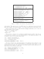
The figure 1.1 presents the NISP methodology. The process requires that the user has a
numerical solver, which has the form Y = f (X), where X are input uncertain parameters and Y
are output random variables. The method is based on the following steps.
• We begin by defining normalized random variables ξ. For example, we may use a random
variables in the interval [0, 1] or a Normal random variable with mean 0 and variance 1. This
choice allows to define the basis for the polynomial chaos, denoted by {Ψk }k≥0 . Depending
on the type of random variable, the polynomials {Ψk }k≥0 are based on Hermite, Legendre
or Laguerre polynomials.
• We can now define a Design Of Experiments (DOE) and, with random variable transformations rules, we get the physical uncertain parameters X. Several types of DOE are available:
Monte-Carlo, Latin Hypercube Sampling, etc... If N experiments are required, the DOE
define the collection of normalized random variables {ξi }i=1,N . Transformation rules allows
to compute the uncertain parameters {Xi }i=1,N , which are the input of the numerical solver
f.
• We can now perform the simulations, that is compute the collection of outputs {Yi }i=1,N
where Yi = f (Xi ).
• The variables Y are then projected on the polynomial basis and the coefficients yk are
computed by integration or regression.
Random
Variable
ξ
Uncertain
Parameter
X
Numerical
Solver
Y=f(X)
Spectral
Projection
Y = Σ y ψ(ξ)
Figure 1.1: The NISP methodology
1.3
The NISP module
The NISP toolbox is available under the following operating systems:
• Linux 32 bits,
• Linux 64 bits,
• Windows 32 bits,
• Mac OS X.
The following list presents the features provided by the NISP toolbox.
4
• Manage various types of random variables:
– uniform,
– normal,
– exponential,
– log-normal.
• Generate random numbers from a given random variable,
• Transform an outcome from a given random variable into another,
• Manage various Design of Experiments for sets of random variables,
– Monte-Carlo,
– Sobol,
– Latin Hypercube Sampling,
– various samplings based on Smolyak designs.
• Manage polynomial chaos expansion and get specific outputs, including
– mean,
– variance,
– quantile,
– correlation,
– etc...
• Generate the C source code which computes the output of the polynomial chaos expansion.
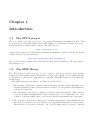
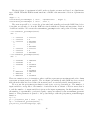
This User’s Manual completes the online help provided with the toolbox, but does not replace
it. The goal of this document is to provide both a global overview of the toolbox and to give some
details about its implementation. The detailed calling sequence of each function is provided by
the online help and will not be reproduced in this document. The inline help is presented in the
figure 1.2.
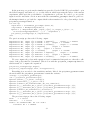
For example, in order to access to the help associated with the randvar class, we type the
following statements in the Scilab console.
help randvar
The previous statements opens the Help Browser and displays the helps page presented in figure
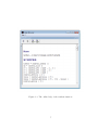
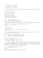
Several demonstration scripts are provided with the toolbox and are presented in the figure
1.4. These demonstrations are available under the ”?” question mark in the menu of the Scilab
console.
Finally, the unit tests provided with the toolbox cover all the features of the toolbox. When
we want to know how to use a particular feature and do not find the information, we can search
in the unit tests which often provide the answer.
5
Figure 1.2: The NISP inline help.
6
Figure 1.3: The online help of the randvar function.
7
Figure 1.4: Demonstrations provided with the NISP toolbox.
8
Chapter 2
Installation
In this section, we present the installation process for the toolbox. We present the steps which
are required to have a running version of the toolbox and presents the several checks which can
be performed before using the toolbox.
2.1
Introduction
There are two possible ways of installing the NISP toolbox in Scilab:
• use the ATOMS system and get a binary version of the toolbox,
• build the toolbox from the sources.
The next two sections present these two ways of using the toolbox.
Before getting into the installation process, let us present some details of the the internal
components of the toolbox. The following list is an overview of the content of the directories:
• tbxnisp/demos : demonstration scripts
• tbxnisp/doc : the documentation
• tbxnisp/doc/usermanual : the LATEXsources of this manual
• tbxnisp/etc : startup and shutdow scripts for the toolbox
• tbxnisp/help : inline help pages
• tbxnisp/macros : Scilab macros files *.sci
• tbxnisp/sci gateway : the sources of the gateway
• tbxnisp/src : the sources of the NISP library
• tbxnisp/tests : tests
• tbxnisp/tests/nonreg tests : tests after some bug has been identified
• tbxnisp/tests/unit tests : unit tests
The current version is based on the NISP Library v2.1.
9
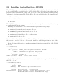
2.2
Installing the toolbox from ATOMS
The ATOMS component is the Scilab tool which allows to search, download, install and load
toolboxes. ATOMS comes with Scilab v5.2. The Scilab-NISP toolbox has been packaged and is
provided mainly by the ATOMS component. The toolbox is provided in binary form, depending
on the user’s operating system. The Scilab-NISP toolbox is available for the following platforms:
• Windows 32 bits,
• Linux 32 bits, 64 bits,
• Mac OS X.
The ATOMS component allows to use a toolbox based on compiled source code, without having
a compiler installed in the system.
Installing the Scilab-NISP toolbox from ATOMS requires the following steps:
• atomsList(): prints the list of current toolboxes,
• atomsShow(): prints informations about a toolbox,
• atomsInstall(): installs a toolbox on the system,
• atomsLoad(): loads a toolbox.
Once installed and loaded, the toolbox will be available on the system from session to session, so
that there is no need to load the toolbox again: it will be available right from the start of the
session.
In the following Scilab session, we use the atomsList() function to print the list of all ATOMS
toolboxes.
--> atomsList ()
ANN_Toolbox - ANN Toolbox
dde_toolbox - Dynamic Data Exchange client for Scilab
module_lycee - Scilab pour les lyc~
Al’es
NISP - Non Intrusive Spectral Projection
plotlib - " Matlab - like " Plotting library for Scilab
scipad - Scipad 7.20
sndfile_toolbox - Read & write sound files
stixbox - Statistics toolbox for Scilab 5.2
In the following Scilab session, we use the atomsShow() function to print the details about
the NISP toolbox.
--> atomsShow (" NISP ")
Package : NISP
Title : NISP
Summary : Non Intrusive Spectral Projection
Version : 2.1
Depend : Category ( ies ) : Optimization
Maintainer ( s ) : Pierre Marechal < pierre . marechal@scilab . org >
Michael Baudin < michael . baudin@scilab . org >
10
Entity : CEA / DIGITEO
WebSite :
License : LGPL
Scilab Version : >= 5.2.0
Status : Not installed
Description : This toolbox allows to approximate a given model ,
which is associated with input random variables .
This toolbox has been created in the context of the
OPUS project :
http :// opus - project . fr /
within the workpackage 2.1.1:
" Construction de m~
Al’ta- mod ~
A ĺles "
This project has received funding by Agence Nationale
de la recherche :
http :// www . agence - nationale - recherche . fr /
See in the help provided in the help / en_US directory
of the toolbox for more information about its use .
Use cases are presented in the demos directory .
In the following Scilab session, we use the atomsInstall() function to download and install
the binary version of the toolbox corresponding to the current operating system.
--> atomsInstall ( " NISP " )
ans =
! NISP 2.1 allusers D :\ Programs \ SC3623 ~1\ contrib \ NISP \2.1
I
!
The "allusers" option of the atomsInstall function can be used to install the toolbox for all
the users of this computer. We finally load the toolbox with the atomsLoad() function.
--> atomsLoad (" NISP ")
Start NISP Toolbox
Load gateways
Load help
Load demos
ans =
! NISP 2.1 D :\ Programs \ SC3623 ~1\ contrib \ NISP \2.1
!
Now that the toolbox is loaded, it will be automatically loaded at the next Scilab session.
2.3
Installing the toolbox from the sources
In this section, we present the steps which are required in order to install the toolbox from the
sources.
In order to install the toolbox from the sources, a compiler is required to be installed on the
machine. This toolbox can be used with Scilab v5.1 and Scilab v5.2. We suppose that the archive
has been unpacked in the ”tbxnisp” directory. The following is a short list of the steps which are
required to setup the toolbox.
1. build the toolbox : run the tbxnisp/builder.sce script to create the binaries of the library,
create the binaries for the gateway, generate the documentation
2. load the toolbox : run the tbxnisp/load.sce script to load all commands and setup the
documentation
11
3. setup the startup configuration file of your Scilab system so that the toolbox is known at
startup (see below for details),
4. run the unit tests : run the tbxnisp/runtests.sce script to perform all unit tests and check
that the toolbox is OK
5. run the demos : run the tbxnisp/rundemos.sce script to run all demonstration scripts and
get a quick interactive overview of its features
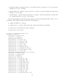
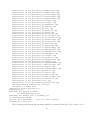
The following script presents the messages which are generated when the builder of the toolbox
is launched. The builder script performs the following steps:
• compile the NISP C++ library,
• compile the C++ gateway library (the glue between the library and Scilab),
• generate the Java help files from the .xml files,
• generate the loader script.
--> exec C :\ tbxnisp \ builder . sce ;
Building sources ...
Generate a loader file
Generate a Makefile
Running the Makefile
Compilation of utils . cpp
Compilation of blas1_d . cpp
Compilation of dcdflib . cpp
Compilation of faure . cpp
Compilation of halton . cpp
Compilation of linpack_d . cpp
Compilation of niederreiter . cpp
Compilation of reversehalton . cpp
Compilation of sobol . cpp
Building shared library ( be patient )
Generate a cleaner file
Generate a loader file
Generate a Makefile
Running the Makefile
Compilation of nisp_gc . cpp
Compilation of nisp_gva . cpp
Compilation of nisp_ind . cpp
Compilation of nisp_index . cpp
Compilation of nisp_inv . cpp
Compilation of nisp_math . cpp
Compilation of nisp_msg . cpp
Compilation of nisp_conf . cpp
Compilation of nisp_ort . cpp
Compilation of nisp_pc . cpp
Compilation of nisp_polyrule . cpp
12
Compilation of nisp_qua . cpp
Compilation of nisp_random . cpp
Compilation of nisp_smo . cpp
Compilation of nisp_util . cpp
Compilation of nisp_va . cpp
Compilation of nisp_smolyak . cpp
Building shared library ( be patient )
Generate a cleaner file
Building gateway ...
Generate a gateway file
Generate a loader file
Generate a Makefile : Makelib
Running the makefile
Compilation of nisp_gettoken . cpp
Compilation of nisp_gwsupport . cpp
Compilation of n i s p _ P o l y n o m i a l C h a o s _ m a p . cpp
Compilation of n i s p _ R a n d o m V a r i a b l e _ m a p . cpp
Compilation of n i s p _ S e t R a n d o m V a r i a b l e _ m a p . cpp
Compilation of sci_nisp_startup . cpp
Compilation of sci_nisp_shutdown . cpp
Compilation of s c i _ n i s p _ v e r b o s e l e v e l s e t . cpp
Compilation of s c i _ n i s p _ v e r b o s e l e v e l g e t . cpp
Compilation of sci_nisp_initseed . cpp
Compilation of sci_randvar_new . cpp
Compilation of sci_ran dvar_de stroy . cpp
Compilation of sci_randvar_size . cpp
Compilation of sci_randvar_tokens . cpp
Compilation of sci_randvar_getlog . cpp
Compilation of sc i_r an dva r_ get val ue . cpp
Compilation of sci_setrandvar_new . cpp
Compilation of s ci _ se tr a nd va r _t o ke ns . cpp
Compilation of sci_set randvar _size . cpp
Compilation of s c i _ se t r a n dv a r _ de s t r o y . cpp
Compilation of s c i _ s e t r a n d v a r _ f r e e m e m o r y . cpp
Compilation of s c i _ s e t r a n d v a r _ a d d r a n d v a r . cpp
Compilation of s ci _ se tr a nd va r _g e tl og . cpp
Compilation of s c i _ s e t r a n d v a r _ g e t d i m e n s i o n . cpp
Compilation of s c i _ se t r a n dv a r _ ge t s i z e . cpp
Compilation of s c i _ s e t r a n d v a r _ g e t s a m p l e . cpp
Compilation of s c i _ s e t r a n d v a r _ s e t s a m p l e . cpp
Compilation of sci_set randvar _save . cpp
Compilation of s c i _ s e t r a n d v a r _ b u i l d s a m p l e . cpp
Compilation of sci_polychaos_new . cpp
Compilation of s ci _ po ly c ha os _ de s tr oy . cpp
Compilation of sc i_p ol ych ao s_t oke ns . cpp
Compilation of sci_polychaos_size . cpp
Compilation of s c i _ p o l y c h a o s _ s e t d e g r e e . cpp
Compilation of s c i _ p o l y c h a o s _ g e t d e g r e e . cpp
Compilation of s c i _ p o l y c h a o s _ f r e e m e m o r y . cpp
13
Compilation of s c i _ p o l y c h a o s _ g e t d i m o u t p u t . cpp
Compilation of s c i _ p o l y c h a o s _ s e t d i m o u t p u t . cpp
Compilation of s c i _ p o l y c h a o s _ g e t s i z e t a r g e t . cpp
Compilation of s c i _ p o l y c h a o s _ s e t s i z e t a r g e t . cpp
Compilation of s c i _ p o l y c h a o s _ f r e e m e m t a r g e t . cpp
Compilation of s c i _ p o l y c h a o s _ s e t t a r g e t . cpp
Compilation of s c i _ p o l y c h a o s _ g e t t a r g e t . cpp
Compilation of s c i _ p o l y c h a o s _ g e t d i m i n p u t . cpp
Compilation of s c i _ p o l y c h a o s _ g e t d i m e x p . cpp
Compilation of sc i_p ol ych ao s_g etl og . cpp
Compilation of s c i _ p o l y c h a o s _ c o m p u t e e x p . cpp
Compilation of s ci _ po ly c ha os _ ge t me an . cpp
Compilation of s c i _ p o l y c h a o s _ g e t v a r i a n c e . cpp
Compilation of s c i _ p o l y c h a o s _ g e t c o v a r i a n c e . cpp
Compilation of s c i _ p o l y c h a o s _ g e t c o r r e l a t i o n . cpp
Compilation of s c i _ p o l y c h a o s _ g e t i n d e x f i r s t . cpp
Compilation of s c i _ p o l y c h a o s _ g e t i n d e x t o t a l . cpp
Compilation of s c i _ p o l y c h a o s _ g e t m u l t i n d . cpp
Compilation of s c i _ p o l y c h a o s _ g e t g r o u p i n d . cpp
Compilation of s c i _ p o l y c h a o s _ s e t g r o u p e m p t y . cpp
Compilation of s c i _ p o l y c h a o s _ g e t g r o u p i n t e r . cpp
Compilation of s c i _ p o l y c h a o s _ g e t i n v q u a n t i l e . cpp
Compilation of s c i _ p o l y c h a o s _ b u i l d s a m p l e . cpp
Compilation of s c i _ p o l y c h a o s _ g e t o u t p u t . cpp
Compilation of s c i _ p o l y c h a o s _ g e t q u a n t i l e . cpp
Compilation of s c i _ p o l y c h a o s _ g e t q u a n t w i l k s . cpp
Compilation of s c i _ p o l y c h a o s _ g e t s a m p l e . cpp
Compilation of s c i _ p o l y c h a o s _ s e t g r o u p a d d v a r . cpp
Compilation of s c i _ p o l y c h a o s _ c o m p u t e o u t p u t . cpp
Compilation of s c i _ po l y c h ao s _ s et i n p u t . cpp
Compilation of s c i _ p o l y c h a o s _ p r o p a g a t e i n p u t . cpp
Compilation of s c i _ po l y c h ao s _ g et a n o v a . cpp
Compilation of s c i _ po l y c h ao s _ s et a n o v a . cpp
Compilation of s c i _ p o l y c h a o s _ g e t a n o v a o r d . cpp
Compilation of s c i _ p o l y c h a o s _ g e t a n o v a o r d c o . cpp
Compilation of s c i _ p o l y c h a o s _ r e a l i s a t i o n . cpp
Compilation of sci_polychaos_save . cpp
Compilation of s c i _ p o l y c h a o s _ g e n e r a t e c o d e . cpp
Building shared library ( be patient )
Generate a cleaner file
Generating loader_gateway . sce ...
Building help ...
Building the master document :
C :\ tbxnisp \ help \ en_US
Building the manual file [ javaHelp ] in
C :\ tbxnisp \ help \ en_US .
( Please wait building ... this can take a while )
Generating loader . sce ...
The following script presents the messages which are generated when the loader of the toolbox
14
is launched. The loader script performs the following steps:
• load the gateway (and the NISP library),
• load the help,
• load the demo.
--> exec C :\ tbxnisp \ loader . sce ;
Start NISP Toolbox
Load gateways
Load help
Load demos
It is now necessary to setup your Scilab system so that the toolbox is loaded automatically
at startup. The way to do this is to configure the Scilab startup configuration file. The directory
where this file is located is stored in the Scilab variable SCIHOME. In the following Scilab session,
we use Scilab v5.2.0-beta-1 in order to know the value of the SCIHOME global variable.
--> SCIHOME
SCIHOME =
C :\ Users \ baudin \ AppData \ Roaming \ Scilab \ scilab -5.2.0 - beta -1
On my Linux system, the Scilab 5.1 startup file is located in
/home/myname/.Scilab/scilab-5.1/.scilab.
On my Windows system, the Scilab 5.1 startup file is located in
C:/Users/myname/AppData/Roaming/Scilab/scilab-5.1/.scilab.
This file is a regular Scilab script which is automatically loaded at Scilab’s startup. If that file
does not already exist, create it. Copy the following lines into the .scilab file and configure the
path to the toolboxes, stored in the SCILABTBX variable.
exec (" C :\ tbxnisp \ loader . sce ");
The following script presents the messages which are generated when the unit tests script of
the toolbox is launched.
--> exec C :\ tbxnisp \ runtests . sce ;
Tests beginning the 2009/11/18 at 12:47:45
TMPDIR = C :\ Users \ baudin \ AppData \ Local \ Temp \ SCI_TMP_6372_
001/004 - [ tbxnisp ] nisp .................. passed : ref created
002/004 - [ tbxnisp ] polychaos1 ............ passed : ref created
003/004 - [ tbxnisp ] randvar1 .............. passed : ref created
004/004 - [ tbxnisp ] setrandvar1 ........... passed : ref created
-------------------------------------------------------------Summary
tests
4 - 100 %
passed
0 0 %
failed
0 0 %
skipped
0 0 %
length
3.84 sec
-------------------------------------------------------------Tests ending the 2009/11/18 at 12:47:48\ end { verbatim }
15
Chapter 3
Configuration functions
In this section, we present functions which allow to configure the NISP toolbox.
The nisp_* functions allows to configure the global behaviour of the toolbox. These functions allows to startup and shutdown the toolbox and initialize the seed of the random number
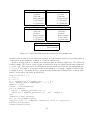
generator. They are presented in the figure 3.1.
nisp_startup ()
Starts up the NISP toolbox.
nisp_shutdown ()
Shuts down the NISP toolbox.
level = nisp_verboselevelget () Returns the current verbose level.
nisp_verboselevelset ( level )
Sets the value of the verbose level.
nisp_initseed ( seed )
Sets the seed of the uniform random number generator.
nisp_destroyall
Destroy all current objects.
nisp_getpath
Returns the path to the current module.
nisp_printall
Prints all current objects.
Figure 3.1: Outline of the configuration methods.
The user has no need to explicitely call the nisp_startup () and nisp_shutdown () functions. Indeed, these functions are called automatically by the etc/NISP.start and etc/NISP.quit
scripts, located in the toolbox directory structure.
The nisp_initseed ( seed ) is especially useful when we want to have reproductible results. It allows to set the seed of the generator at a particular value, so that the sequence of
uniform pseudo-random numbers is deterministic. When the toolbox is started up, the seed is
automatically set to 0, which allows to get the same results from session to session.
16
Chapter 4
The randvar class
In this section, we present the randvar class, which allows to define a random variable, and to
generate random numbers from a given distribution function.
4.1
The distribution functions
In this section, we present the distribution functions provided by the randvar class. We especially
present the Log-normal distribution function.
4.1.1
Overview
The table ?? gives the list of distribution functions which are available with the randvar class
[1].
Each distribution functions have zero, one or two parameters. One random variable can be
specified by giving explicitely its parameters or by using default parameters. The parameters for
all distribution function are presented in the figure ??, which also presents the conditions which
must be satisfied by the parameters.
Name
”Normale”
”Uniforme”
”Exponentielle”
”LogNormale”
”LogUniforme”
f (x)
2σ
1
√
exp
2π
1
b−a ,
2
− 12 (x−µ)
σ2
if x ∈ [a, b[
0
if
x∈
/ [a, b[
λ exp (−λx) , if x > 0
if x ≤ 0 ( 0
2
1
1 (ln(x)−µ)
√
exp − 2
,
σ2
σx 2π
0
1
1
if x ∈ [a, b[
x ln(b)−ln(a) ,
0
if x ∈
/ [a, b[
if x > 0
if x ≤ 0
E(X)
V (X)
µ
σ2
b+a
2
(b−a)2
12
1
λ
1
λ2
exp µ + 12 σ 2
b−a
ln(b)−ln(a)
exp(σ 2 ) − 1 exp 2µ + σ 2
1
b2 −a2
2 ln(b)−ln(a)
− E(x)
Figure 4.1: Distributions functions of the randvar class. – The expected value is denoted by
E(X) and the variance is denoted by V (X).
17
Name
”Normale”
”Uniforme”
”Exponentielle”
”LogNormale”
”LogUniforme”
Parameter #1 : a Parameter #2 : b
µ = 0.
σ = 1.
a = 0.
b = 1.
λ = 1.
0
µ = 0.1
σ = 1.0
a = 0.1
b = 1.0
Conditions
σ>0
a<b
µ0 , σ > 0
a, b > 0, a < b
Figure 4.2: Default parameters for distributions functions.
4.1.2
Parameters of the Log-normal distribution
For the ”LogNormale” law, the distribution function is usually defined by the expected value µ
and the standard deviation σ of the underlying Normal random variable. But, when we create
a LogNormale randvar, the parameters to pass to the constructor are the expected value of the
LogNormal random variable E(X) and the standard deviation of the underlying Normale random
variable σ. The expected value and the variance of the Log Normal law are given by
1 2
(4.1)
E(X) = exp µ + σ
2
V (X) = exp(σ 2 ) − 1 exp 2µ + σ 2 .
(4.2)
It is possible to invert these formulas, in the situation where the given parameters are the expected
value and the variance of the Log Normal random variable. We can invert completely the previous
equations and get
V (X)
1
(4.3)
µ = ln(E(X)) − ln 1 +
2
E(X)2
V (X)
2
σ = ln 1 +
.
(4.4)
E(X)2
In particular, the expected value µ of with the Normal random variable satisfies the equation
µ = ln(E(X)) − σ 2 .
4.1.3
(4.5)
Uniform random number generation
In this section, we present the generation of uniform random numbers.
The goal of this section is to warn users about a current limitation of the library. Indeed, the
random number generator is based on the compiler, so that its quality cannot be guaranted.
The Uniforme law is associated with the parameters a, b ∈ R with a < b. It produces real
values uniform in the interval [a, b].
To compute the uniform random number X in the interval [a, b], a uniform random number
in the interval [0, 1] is generated and then scaled with
X = a + (b − a)X.
(4.6)
Let us now analyse how the uniform random number X ∈ [0, 1] is computed. The uniform
random generator is based on the C function rand, which returns an integer n in the interval
18
[0, RAN D M AX[. The value of the RAN D M AX variable is defined in the file stdlib.h and is
compiler-dependent. For example, with the Visual Studio C++ 2008 compiler, the value is
RAN D M AX = 215 − 1 = 32767.
(4.7)
A uniform value X in the range [0, 1[ is computed from
X=
n
,
N
(4.8)
where N = RAN D M AX and n ∈ [0, RAN D M AX[.
4.2
Methods
In this section, we give an overview of the methods which are available in the randvar class.
4.2.1
Overview
The figure ?? presents the methods available in the randvar class. The inline help contains the
detailed calling sequence for each function and will not be repeated here.
Constructors
rv = randvar_new ( type [, options])
Methods
value = randvar_getvalue ( rv [, options] )
randvar_getlog ( rv )
Destructor
randvar_destroy ( rv )
Static methods
rvlist = randvar_tokens ()
nbrv = randvar_size ()
Figure 4.3: Outline of the methods of the randvar class.
4.2.2
The Oriented-Object system
In this section, we present the token system which allows to emulate an oriented-object programming with Scilab. We also present the naming convention we used to create the names of the
functions.
The randvar class provides the following functions.
• The constructor function randvar_new allows to create a new random variable and returns
a token rv.
• The method randvar_getvalue takes the token rv as its first argument. In fact, all methods
takes as their first argument the object on which they apply.
19
• The destructor randvar_destroy allows to delete the current object from the memory of
the library.
• The static methods randvar_tokens and randvar_size allows to quiery the current object
which are in use. More specifically, the randvar_size function returns the number of current
randvar objects and the randvar_tokens returns the list of current randvar objects.
In the following Scilab sessions, we present these ideas with practical uses of the toolbox.
Assume that we start Scilab and that the toolbox is automatically loaded. At startup, there
are no objects, so that the randvar_size function returns 0 and the randvar_tokens function
returns an empty matrix.
--> nb = randvar_size ()
nb =
0.
--> tokenmatrix = randvar_tokens ()
tokenmatrix =
[]
We now create 3 new random variables, based on the Uniform distribution function. We store
the tokens in the variables vu1, vu2 and vu3. These variables are regular Scilab double precision
floating point numbers. Each value is a token which represents a random variable stored in the
toolbox memory space.
--> vu1 = randvar_new ( " Uniforme " )
vu1 =
0.
--> vu2 = randvar_new ( " Uniforme " )
vu2 =
1.
--> vu3 = randvar_new ( " Uniforme " )
vu3 =
2.
There are now 3 objects in current use, as indicated by the following statements. The
tokenmatrix is a row matrix containing regular double precision floating point numbers.
--> nb = randvar_size ()
nb =
3.
--> tokenmatrix = randvar_tokens ()
tokenmatrix =
0.
1.
2.
We assume that we have now made our job with the random variables, so that it is time
to destroy the random variables. We call the randvar_destroy functions, which destroys the
variables.
--> randvar_destroy ( vu1 );
--> randvar_destroy ( vu2 );
--> randvar_destroy ( vu3 );
We can finally check that there are no random variables left in the memory space.
20
--> nb = randvar_size ()
nb =
0.
--> tokenmatrix = randvar_tokens ()
tokenmatrix =
[]
Scilab is a wonderful tool to experiment algorithms and make simulations. It happens sometimes that we are managing many variables at the same time and it may happen that, at some
point, we are lost. The static methods provides tools to be able to recover from such a situation
without closing our Scilab session.
In the following session, we create two random variables.
--> vu1 = randvar_new ( " Uniforme " )
vu1 =
3.
--> vu2 = randvar_new ( " Uniforme " )
vu2 =
4.
Assume now that we have lost the token associated with the variable vu2. We can easily simulate
this situation, by using the clear, which destroys a variable from Scilab’s memory space.
--> clear vu2
--> randvar_getvalue ( vu2 )
! - - error 4
Undefined variable : vu2
It is now impossible to generate values from the variable vu2. Moreover, it may be difficult to
know exactly what went wrong and what exact variable is lost. At any time, we can use the
randvar_tokens function in order to get the list of current variables. Deleting these variables
allows to clean the memory space properly, without memory loss.
--> randvar_tokens ()
ans =
3.
4.
--> randvar_destroy (3)
ans =
3.
--> randvar_destroy (4)
ans =
4.
--> randvar_tokens ()
ans =
[]
4.3
Examples
In this section, we present to examples of use of the randvar class. The first example presents
the simulation of a Normal random variable and the generation of 1000 random variables. The
second example presents the transformation of a Uniform outcome into a LogUniform outcome.
21
4.3.1
A sample session
We present a sample Scilab session, where the randvar class is used to generate samples from the
Normale law.
In the following Scilab session, we create a Normale random variable and compute samples
from this law. The nisp_initseed function is used to initialize the seed for the uniform random
variable generator. Then we use the randvar_new function to create a new random variable from
the Normale law with mean 1. and standard deviation 0.5. The main loop allows to compute
1000 samples from this law, based on calls to the randvar_getvalue function. Once the samples
are computed, we use the Scilab function mean to check that the mean is close to 1 (which is
the expected value of the Normale law, when the number of samples is infinite). Finally, we use
the randvar_destroy function to destroy our random variable. Once done, we plot the empirical
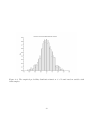
distribution function of this sample, with 50 classes.
nisp_initseed ( 0 );
mu = 1.0;
sigma = 0.5;
rv = randvar_new ( " Normale " , mu , sigma );
nbshots = 1000;
values = zeros ( nbshots );
for i =1: nbshots
values ( i ) = randvar_getvalue ( rv );
end
mymean = mean ( values );
mysigma = st_deviation ( values );
myvariance = variance ( values );
mprintf ( " Mean is : %f ( expected = %f )\ n " , mymean , mu );
mprintf ( " Standard deviation is : %f ( expected = %f )\ n " , mysigma , sigma );
mprintf ( " Variance is : %f ( expected = %f )\ n " , myvariance , sigma ^2);
randvar_destroy ( rv );
histplot (50 , values )
xtitle ( " Empirical normal probability distribution function " ," X " ," P ( x ) " )
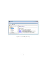
The previous script produces the following output.
Mean is : 0.988194 ( expected = 1.000000)
Standard deviation is : 0.505186 ( expected = 0.500000)
Variance is : 0.255213 ( expected = 0.250000)
4.3.2
Variable transformations
In this section, we present the transformation of uniform random variables into other types of
variables. The transformations which are available in the randvar class are presented in figure
??. We begin the analysis by a presentation of the theory required to perform transformations.
Then we present some of the many the transformations which are provided by the library.
We now present some additionnal details for the function randvar_getvalue ( rv , rv2 ,
value2 ). This method allows to transform a random variable sample from one law to another.
The statement
value = randvar_getvalue ( rv , rv2 , value2 )
22
Figure 4.4: The empirical probability distribution function of a Normal random variable with
1000 samples.
23
Source
Normale
Target
Source
LogNormale
Normale
Uniforme
Exponentielle
LogNormale
LogUniforme
Source
Uniforme
Target
Target
Normale
Uniforme
Exponentielle
LogNormale
LogUniforme
Source
LogUniforme
Uniforme
Normale
Exponentielle
LogNormale
LogUniforme
Target
Uniforme
Normale
Exponentielle
LogNormale
LogUniforme
Source
Exponentielle
Target
Exponentielle
Figure 4.5: Variable transformations available in the randvar class.
returns a random value from the distribution function of the random variable rv by transformation
of value2 from the distribution function of random variable rv2.
In the following session, we transform a uniform random variable sample into a LogUniform
variable sample. We begin to create a random variable rv from a LogUniform law and parameters
a = 10, b = 20. Then we create a second random variable rv2 from a Uniforme law and parameters
a = 2, b = 3. The main loop is based on the transformation of a sample computed from rv2 into
a sample from rv. The mean allows to check that the transformed samples have an mean value
which corresponds to the random variable rv.
nisp_initseed ( 0 );
a = 10.0;
b = 20.0;
rv = randvar_new ( " LogUniforme " , a , b );
rv2 = randvar_new ( " Uniforme " , 2 , 3 );
nbshots = 1000;
values = zeros ( nbshots );
for i =1: nbshots
value2 = randvar_getvalue ( rv2 );
values ( i ) = randvar_getvalue ( rv , rv2 , value2 );
end
computed = mean ( values );
mu = (b - a )/( log ( b ) - log ( a ))
expected = mu ; // " computed " should be close to " expected "
randvar_destroy ( rv );
randvar_destroy ( rv2 );
24
The transformation depends on the mother random variable rv1 and on the daughter random variable rv. Specific transformations are provided for all many combinations of the two
distribution functions. These transformations will be analysed in the next sections.
25
Chapter 5
The setrandvar class
In this chapter, we presen the setrandvar class. The first section gives a brief outline of the
features of this class and the second section present several examples.
5.1
Introduction
The setrandvar class allows to manage a collection of random variables and to build a Design
Of Experiments (DOE). Several types of DOE are provided:
• Monte-Carlo,
• Latin Hypercube Sampling,
• Smolyak.
Once a DOE is created, we can retrieve the information experiment by experiment or the whole
matrix of experiments. This last feature allows to benefit from the fact that Scilab can natively
manage matrices, so that we do not have to perform loops to manage the complete DOE. Hence,
good performances can be observed, even if the language still is interpreted.
The figure 5.1 presents the methods available in the setrandvar class. A complete description
of the input and output arguments of each function is available in the inline help and will not be
repeated here.
More informations about the Oriented Object system used in this toolbox can be found in the
section ??.
5.2
Examples
In this section, we present examples of use of the setrandvar class. In the first example, we
present a Scilab session where we create a Latin Hypercube Sampling. In the second part, we
present various types of DOE which can be generated with this class.
5.2.1
A LHS design
In this section, we present the creation of a Latin Hypercube Sampling. In our example, the DOE
is based on two random variables, the first being Normal with mean 1.0 and standard deviation
0.5 and the second being Uniform in the interval [2, 3].
26
Constructors
srv = setrandvar_new ( )
srv = setrandvar_new ( n )
srv = setrandvar_new ( file )
Methods
setrandvar_setsample ( srv , name , np )
setrandvar_setsample ( srv , k , i , value )
setrandvar_setsample ( srv , k , value )
setrandvar_setsample ( srv , value )
setrandvar_save ( srv , file )
np = setrandvar_getsize ( srv )
sample = setrandvar_getsample ( srv , k , i )
sample = setrandvar_getsample ( srv , k )
sample = setrandvar_getsample ( srv )
setrandvar_getlog ( srv )
nx = setrandvar_getdimension ( srv )
setrandvar_freememory ( srv )
setrandvar_buildsample ( srv , srv2 )
setrandvar_buildsample ( srv , name , np )
setrandvar_buildsample ( srv , name , np , ne )
setrandvar_addrandvar ( srv , rv )
Destructor
setrandvar_destroy ( srv )
Static methods
tokenmatrix = setrandvar_tokens ()
nb = setrandvar_size ()
Figure 5.1: Outline of the methods of the setrandvar class
27
We begin by defining two random variables with the randvar_new function.
vu1 = randvar_new ( " Normale " ,1.0 ,0.5);
vu2 = randvar_new ( " Uniforme " ,2.0 ,3.0);
Then, we create a collection of random variables with the setrandvar_new function which
creates here an empty collection of random variables. Then we add the two random variables to
the collection.
srv = setrandvar_new ( );
setrandvar_ ad d ra nd v ar ( srv , vu1 );
setrandvar_ ad d ra nd v ar ( srv , vu2 );
We can now build the DOE so that it is a LHS sampling with 1000 experiments.
setrandvar _ b u i ld s a m pl e ( srv , " Lhs " , 1000 );
At this point, the DOE is stored in the memory space of the NISP library, but we do not have
a direct access to it. We now call the setrandvar_getsample function and store that DOE into
the sampling matrix.
sampling = s etr an dva r_g et sam pl e ( srv );
The sampling matrix has 1000 rows, corresponding to each experiment, and 2 columns, corresponding to each input random variable.
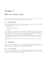
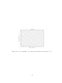
The following script allows to plot the sampling, which is is presented in figure 5.2.
wnum = 100001
my_handle
= scf ( wnum );
clf ( my_handle , " reset " );
plot ( sampling (: ,1) , sampling (: ,2));
my_handle . children . children . children . line_mode =
my_handle . children . children . children . mark_mode =
my_handle . children . children . children . mark_size =
my_handle . children . title . text = " Latin Hypercube
my_handle . children . x_label . text = " Variable #1 :
my_handle . children . y_label . text = " Variable #2 :
" off " ;
" on " ;
2;
Sampling " ;
Normale ,1.0 ,0.5 " ;
Uniforme ,2.0 ,3.0 " ;
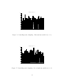
The following script allows to plot the histogram of the two variables, which are presented in
figures 5.3 and 5.4.
// Plot Var #1
wnum = 100002
my_handle
= scf ( wnum );
clf ( my_handle , " reset " );
histplot ( 50 , sampling (: ,1))
my_handle . children . title . text = " Variable #1 : Normale ,1.0 ,0.5 " ;
// Plot Var #2
wnum = 100003
my_handle
= scf ( wnum );
clf ( my_handle , " reset " );
histplot ( 50 , sampling (: ,2))
my_handle . children . title . text = " Variable #2 : Uniforme ,2.0 ,3.0 " ;
We can use the mean and variance on each random variable and check that the expected
result is computed. We insist on the fact that the mean and variance functions are not provided
28
Figure 5.2: Latin Hypercube Sampling - The first variable is Normal, the second variable is
Uniform.
Variable #1 : Normale,1.0,0.5
0.8
0.7
0.6
0.5
0.4
0.3
0.2
0.1
0.0
-1.0
-0.5
0.0
0.5
1.0
1.5
2.0
2.5
3.0
Figure 5.3: Latin Hypercube Sampling - Normal random variable.
29
Variable #2 : Uniforme,2.0,3.0
1.2
1.0
0.8
0.6
0.4
0.2
0.0
2.0
2.1
2.2
2.3
2.4
2.5
2.6
2.7
2.8
2.9
3.0
Figure 5.4: Latin Hypercube Sampling - Uniform random variable (the LHS sampling is not a
Monte-Carlo sampling).
by the NISP library: these are pre-defined functions which are available in the Scilab library. That
means that any Scilab function can be now used to process the data generated by the toolbox.
for ivar = 1:2
m = mean ( sampling (: , ivar ))
mprintf ( " Variable # %d , Mean : %f \ n " , ivar , m )
v = variance ( sampling (: , ivar ))
mprintf ( " Variable # %d , Variance : %f \ n " , ivar , v )
end
The previous script produces the following output.
Variable
Variable
Variable
Variable
#1 ,
#1 ,
#2 ,
#2 ,
Mean : 1.000000
Variance : 0.249925
Mean : 2.500000
Variance : 0.083417
Our numerical simulation is now finished, but we must destroy the objects so that the memory
managed by the toolbox is deleted.
randvar_destroy ( vu1 )
randvar_destroy ( vu2 )
setrandvar_destroy ( srv )
5.2.2
Other types of DOE
The following Scilab session allows to generate a Monte-Carlo sampling with two uniform variables
in the interval [−1, 1]. The figure 5.5 presents this sampling and the figures 5.6 and 5.7 present
the histograms of the two uniform random variables.
30
vu1 = randvar_new ( " Uniforme " , -1.0 ,1.0);
vu2 = randvar_new ( " Uniforme " , -1.0 ,1.0);
srv = setrandvar_new ( );
setrandvar_ ad d ra nd v ar ( srv , vu1 );
setrandvar_ ad d ra nd v ar ( srv , vu2 );
setrandvar _ b u i ld s a m pl e ( srv , " MonteCarlo " , 1000 );
sampling = s etr an dva r_g et sam pl e ( srv );
randvar_destroy ( vu1 );
randvar_destroy ( vu2 );
setrandvar_destroy ( srv );
Figure 5.5: Monte-Carlo Sampling - Two uniform variables in the interval [−1, 1].
It is easy to change the type of sampling by modifying the second argument of the setrandvar_buildsa
function. This way, we can create the Petras, Quadrature and Sobol sampling presented in figures
5.8, 5.9 and 5.10.
31
Variable #1 : Uniforme,-1.0,1.0
0.8
0.7
0.6
0.5
0.4
0.3
0.2
0.1
0.0
-1.0
-0.8
-0.6
-0.4
-0.2
0.0
0.2
0.4
0.6
0.8
1.0
Figure 5.6: Latin Hypercube Sampling - First uniform variable in [−1, 1].
Variable #2 : Uniforme,-1.0,1.0
0.8
0.7
0.6
0.5
0.4
0.3
0.2
0.1
0.0
-1.0
-0.8
-0.6
-0.4
-0.2
0.0
0.2
0.4
0.6
0.8
1.0
Figure 5.7: Latin Hypercube Sampling - Second uniform variable in [−1, 1].
32
Figure 5.8: Petras sampling - Two uniform variables in the interval [−1, 1].
Figure 5.9: Quadrature sampling - Two uniform variables in the interval [−1, 1].
33
Figure 5.10: Sobol sampling - Two uniform variables in the interval [−1, 1].
34
Chapter 6
The polychaos class
6.1
Introduction
The polychaos class allows to manage a polynomial chaos expansion. The coefficients of the
expansion are computed based on given numerical experiments which creates the association
between the inputs and the outputs. Once computed, the expansion can be used as a regular
function. The mean, standard deviation or quantile can also be directly retrieved.
The tool allows to get the following results:
• mean,
• variance,
• quantile,
• correlation, etc...
Moreover, we can generate the C source code which computes the output of the polynomial chaos
expansion. This C source code is stand-alone, that is, it is independent of both the NISP library
and Scilab. It can be used as a meta-model.
The figure 6.1 presents the most commonly used methods available in the polychaos class.
More methods are presented in figure 6.2. The inline help contains the detailed calling sequence
for each function and will not be repeated here. More than 50 methods are available and most of
them will not be presented here.
More informations about the Oriented Object system used in this toolbox can be found in the
section ??.
6.2
Examples
In this section, we present to examples of use of the polychaos class.
6.2.1
Product of two random variables
In this section, we present the polynomial expansion of the product of two random variables.
We analyse the Scilab script and present the methods which are available to perform the sensi35
Constructors
pc = polychaos_new ( file )
pc = polychaos_new ( srv , ny )
pc = polychaos_new ( pc , nopt , varopt )
Methods
polychaos_setsizetarget ( pc , np )
polychaos_settarget ( pc , output )
polychaos_setinput ( pc , invalue )
polychaos_setdimoutput ( pc , ny )
polychaos_setdegree ( pc , no )
polychaos_getvariance ( pc )
polychaos_getmean ( pc )
Destructor
polychaos_destroy (pc)
Static methods
tokenmatrix = polychaos_tokens ()
nb = polychaos_size ()
Figure 6.1: Outline of the methods of the polychaos class
tivity analysis. This script is based on the NISP methodology, which has been presented in the
Introduction chapter. We will use the figure 1.1 as a framework and will follow the steps in order.
In the following Scilab script, we define the function Example which takes a vector of size 2 as
input and returns a scalar as output.
function y = Exemple ( x )
y (1) = x (1) * x (2);
endfunction
We now create a collection of two stochastic (normalized) random variables. Since the random variables are normalized, we use the default parameters of the randvar_new function. The
normalized collection is stored in the variable srvx.
vx1 = randvar_new ( " Normale " );
vx2 = randvar_new ( " Uniforme " );
srvx = setrandvar_new ();
setrandvar_ ad d ra nd v ar ( srvx , vx1 );
setrandvar_ ad d ra nd v ar ( srvx , vx2 );
We create a collection of two uncertain parameters. We explicitely set the parameters of each
random variable, that is, the first Normal variable is associated with a mean equal to 1.0 and
a standard deviation equal to 0.5, while the second Uniform variable is in the interval [1.0, 2.5].
This collection is stored in the variable srvu.
vu1 = randvar_new ( " Normale " ,1.0 ,0.5);
vu2 = randvar_new ( " Uniforme " ,1.0 ,2.5);
srvu = setrandvar_new ();
setrandvar_ ad d ra nd v ar ( srvu , vu1 );
setrandvar_ ad d ra nd v ar ( srvu , vu2 );
36
Methods
output = polychaos_gettarget ( pc )
np = polychaos_getsizetarget ( pc )
polychaos_getsample ( pc , k , ovar )
polychaos_getquantile ( pc , k )
polychaos_getsample ( pc )
polychaos_getquantile ( pc , alpha )
polychaos_getoutput ( pc )
polychaos_getmultind ( pc )
polychaos_getlog ( pc )
polychaos_getinvquantile ( pc , threshold )
polychaos_getindextotal ( pc )
polychaos_getindexfirst ( pc )
ny = polychaos_getdimoutput ( pc )
nx = polychaos_getdiminput ( pc )
p = polychaos_getdimexp ( pc )
no = polychaos_getdegree ( pc )
polychaos_getcovariance ( pc )
polychaos_getcorrelation ( pc )
polychaos_getanova ( pc )
polychaos_generatecode ( pc , filename , funname )
polychaos_computeoutput ( pc )
polychaos_computeexp ( pc , srv , method )
polychaos_computeexp ( pc , pc2 , invalue , varopt )
polychaos_buildsample ( pc , type , np , order )
Figure 6.2: More methods from the polychaos class
37
The first design of experiment is build on the stochastic set srvx and based on a Quadrature
type of DOE. Then this DOE is transformed into a DOE for the uncertain collection of parameters
srvu.
degre = 2;
setrandvar _ b u i ld s a m pl e ( srvx , " Quadrature " , degre );
setrandvar _ b u i ld s a m pl e ( srvu , srvx );
The next steps will be to create the polynomial and actually perform the DOE. But before
doing this, we can take a look at the DOE associated with the stochastic and uncertain collection
of random variables. We can use the setrandvar_getsample twice and get the following output.
--> setrandva r_g et sam pl e ( srvx )
ans =
- 1.7320508
0.1127017
- 1.7320508
0.5
- 1.7320508
0.8872983
0.
0.1127017
0.
0.5
0.
0.8872983
1.7320508
0.1127017
1.7320508
0.5
1.7320508
0.8872983
--> setrandva r_g et sam pl e ( srvu )
ans =
0.1339746
0.1339746
0.1339746
1.
1.
1.
1.8660254
1.8660254
1.8660254
1.1690525
1.75
2.3309475
1.1690525
1.75
2.3309475
1.1690525
1.75
2.3309475
These two matrices are a 9×2 matrices, where each line represents an experiment and each column
represents an input random variable. The stochastic (normalized) srvx DOE has been created
first, then the srvu has been deduced from srvx based on random variable transformations.
We now use the polychaos_new function and create a new polynomial pc. The number of
input variables corresponds to the number of variables in the stochastic collection srvx, that is
2, and the number of output variables is given as the input argument ny. In this particular case,
the number of experiments to perform is equal to np=9, as returned by the setrandvar_getsize
function. This parameter is passed to the polynomial pc with the polychaos_setsizetarget
function.
ny = 1;
pc = polychaos_new ( srvx , ny );
np = setrandvar_getsize ( srvx );
polychaos_ s e t s i z e t a r g e t ( pc , np );
38
In the next step, we perform the simulations prescribed by the DOE. We perform this loop in
the Scilab language and make a loop over the index k, which represents the index of the current
experiment, while np is the total number of experiments to perform. For each loop, we get the
input from the uncertain collection srvu with the setrandvar_getsample function, pass it to
the Exemple function, get back the output which is then transferred to the polynomial pc by the
polychaos_settarget function.
for k =1: np
inputdata = s et ran dva r_ get sa mpl e ( srvu , k );
outputdata = Exemple ( inputdata );
mprintf ( " Experiment # %d , input =[ %s ] ,\ t output = %f \ n " , k ,
strcat ( string ( inputdata ) , " " ) , outputdata )
polychaos_s ettarget ( pc ,k , outputdata );
end
The previous script produces the following output.
Experiment
Experiment
Experiment
Experiment
Experiment
Experiment
Experiment
Experiment
Experiment
#1 ,
#2 ,
#3 ,
#4 ,
#5 ,
#6 ,
#7 ,
#8 ,
#9 ,
input
input
input
input
input
input
input
input
input
=[0.1339746 1.1690525] ,
output = 0.156623
=[0.1339746 1.75] , output = 0.234456
=[0.1339746 2.3309475] ,
output = 0.312288
=[1 1.1690525] ,
output = 1.169052
=[1 1.75] , output = 1.750000
=[1 2.3309475] ,
output = 2.330948
=[1.8660254 1.1690525] ,
output = 2.181482
=[1.8660254 1.75] , output = 3.265544
=[1.8660254 2.3309475] ,
output = 4.349607
We can compute the polynomial expansion based on numerical integration so that the coefficients of the polynomial are determined. This is done with the polychaos_computeexp function,
which stands for ”compute the expansion”.
polychaos_se tdegree ( pc , degre );
polychaos_co mpu te exp ( pc , srvx , " Integration " );
Everything is now ready for the sensitivity analysis. Indeed, the polychaos_getmean returns
the mean while the polychaos_getvariance returns the variance.
average = polychaos_getmean ( pc );
var = polyc h ao s_ g et v ar ia n ce ( pc );
mprintf ( " Mean
= %f \ n " , average );
mprintf ( " Variance
= %f \ n " , var );
mprintf ( " Indice de sensibilit ~
A l’ du 1 er ordre \ n " );
mprintf ( "
Variable X1 = %f \ n " , p o l y c h a o s _ g e t i n d e x f i r s t ( pc ,1));
mprintf ( "
Variable X2 = %f \ n " , p o l y c h a o s _ g e t i n d e x f i r s t ( pc ,2));
mprintf ( " Indice de sensibilite Totale \ n " );
mprintf ( "
Variable X1 = %f \ n " , p o l y c h a o s _ g e t i n d e x t o t a l ( pc ,1));
mprintf ( "
Variable X2 = %f \ n " , p o l y c h a o s _ g e t i n d e x t o t a l ( pc ,2));
The previous script produces the following output.
Mean
= 1.750000
Variance
= 1.000000
Indice de sensibilit ~
A l’ du 1 er ordre
Variable X1 = 0.765625
39
Variable X2 = 0.187500
Indice de sensibilite Totale
Variable X1 = 0.812500
Variable X2 = 0.234375
In order to free the memory required for the computation, it is necessary to delete all the
objects created so far.
polychaos_destroy ( pc );
randvar_destroy ( vu1 );
randvar_destroy ( vu2 );
randvar_destroy ( vx1 );
randvar_destroy ( vx2 );
setrandvar_destroy ( srvu );
setrandvar_destroy ( srvx );
6.2.2
The Ishigami test case
In this section, we present the Ishigami test case.
The function Exemple is the model that we consider in this numerical experiment. This
function takes a vector of size 3 in input and returns a scalar output.
function y = Exemple ( x )
a =7.;
b =0.1;
s1 = sin ( x (1));
s2 = sin ( x (2));
y (1) = s1 + a * s2 * s2 + b * x (3)* x (3)* x (3)* x (3)* s1 ;
endfunction
We create 3 uncertain parameters which are uniform in the interval [−π, π] and put these
random variables into the collection srvu.
rvu1 = randvar_new ( " Uniforme " ,- %pi , %pi );
rvu2 = randvar_new ( " Uniforme " ,- %pi , %pi );
rvu3 = randvar_new ( " Uniforme " ,- %pi , %pi );
srvu = setrandvar_new ();
setrandvar_ ad d ra nd v ar ( srvu , rvu1 );
setrandvar_ ad d ra nd v ar ( srvu , rvu2 );
setrandvar_ ad d ra nd v ar ( srvu , rvu3 );
The collection of stochastic variables is created with the function setrandvar_new. The calling
sequence srvx = setrandvar_new( nx ) allows to create a collection of nx=3 random variables
uniform in the interval [0, 1]. Then we create a Petras DOE for the stochastic collection srvx and
transform it into a DOE for the uncertain parameters srvu.
nx = setra n d v a r _ g e t d i m e n s i o n ( srvu );
srvx = setrandvar_new ( nx );
degre = 9;
setrandvar _ b u i ld s a m pl e ( srvx , " Petras " , degre );
setrandvar _ b u i ld s a m pl e ( srvu , srvx );
40
We use the polychaos_new function and create the new polynomial pc with 3 inputs and 1
output.
noutput = 1;
pc = polychaos_new ( srvx , noutput );
The next step allows to perform the simulations associated with the DOE prescribed by the
collection srvu.
np = setrandvar_getsize ( srvu );
polychaos_ s e t s i z e t a r g e t ( pc , np );
for k =1: np
inputdata = s et ran dva r_ get sa mpl e ( srvu , k );
outputdata = Exemple ( inputdata );
polychaos_se ttarget ( pc ,k , outputdata );
end
We can now compute the polynomial expansion by integration.
polychaos_se tdegree ( pc , degre );
polychaos_co mpu te exp ( pc , srvx , " Integration " );
Everything is now ready so that we can do the sensitivy analysis, as in the following script.
average = polychaos_getmean ( pc );
var = polyc h ao s_ g et v ar ia n ce ( pc );
mprintf ( " Mean
= %f \ n " , average );
mprintf ( " Variance
= %f \ n " , var );
mprintf ( " Indice de sensibilit ~
A l’ du 1 er ordre \ n " );
mprintf ( "
Variable X1 = %f \ n " , p o l y c h a o s _ g e t i n d e x f i r s t ( pc ,1));
mprintf ( "
Variable X2 = %f \ n " , p o l y c h a o s _ g e t i n d e x f i r s t ( pc ,2));
mprintf ( "
Variable X3 = %f \ n " , p o l y c h a o s _ g e t i n d e x f i r s t ( pc ,3));
mprintf ( " Indice de sensibilite Totale \ n " );
mprintf ( "
Variable X1 = %f \ n " , p o l y c h a o s _ g e t i n d e x t o t a l ( pc ,1));
mprintf ( "
Variable X2 = %f \ n " , p o l y c h a o s _ g e t i n d e x t o t a l ( pc ,2));
mprintf ( "
Variable X3 = %f \ n " , p o l y c h a o s _ g e t i n d e x t o t a l ( pc ,3));
The previous script produces the following output.
Mean
= 3.500000
Variance
= 13.842473
Indice de sensibilit ~
A l’ du 1 er ordre
Variable X1 = 0.313953
Variable X2 = 0.442325
Variable X3 = 0.000000
Indice de sensibilite Totale
Variable X1 = 0.557675
Variable X2 = 0.442326
Variable X3 = 0.243721
We now focus on the variance generated by the variables #1 and #3. We set the group
to the empty group with the polychaos_setgroupempty function and add variables with the
polychaos_setgroupaddvar function.
groupe = [1 3];
41
polychaos_ s e t g r o u p e m p t y ( pc );
pol ychao s_ s e t g r o u p a d d v a r ( pc , groupe (1) );
pol ychao s_ s e t g r o u p a d d v a r ( pc , groupe (2) );
mprintf ( " Part de la variance d ’ ’ un groupe de variables \ n " );
mprintf ( "
Groupe X1 et X2 = %f \ n " , p ol y ch ao s _g et g ro u pi nd ( pc ));
The previous script produces the following output.
Part de la variance d ’ un groupe de variables
Groupe X1 et X2 =0.557674
The function polychaos_getanova prints the functionnal decomposition of the normalized
variance.
polychaos_getanova ( pc );
The previous script produces the following output.
1
0
1
0
1
0
1
0
1
1
0
0
1
1
0
0
0
1
1
1
1
:
:
:
:
:
:
:
0.313953
0.442325
1.55229 e -009
8.08643 e -031
0.243721
7.26213 e -031
1.6007 e -007
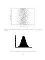
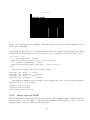
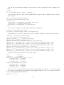
We can compute the density function associated with the output variable of the function. In
order to compute it, we use the polychaos_buildsample function and create a Latin Hypercube
Sampling with 10000 experiments. The polychaos_getsample function allows to quiery the
polynomial and get the outputs. We plot it with the histplot Scilab graphic function, which
produces the figure 6.3.
polychaos_b ui l ds am p le ( pc , " Lhs " ,10000 ,0);
sample_output = polych aos_get sample ( pc );
histplot (50 , sample_output )
xtitle ( " Fonction Ishigami - Histogramme normalis ~
A l’" );
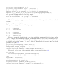
We can plot a bar graph of the sensitivity indices, as presented in figure 6.4.
for i =1: nx
indexfirst ( i )= p o l y c h a o s _ g e t i n d e x f i r s t ( pc , i );
indextotal ( i )= p o l y c h a o s _ g e t i n d e x t o t a l ( pc , i );
end
my_handle = scf (10002);
bar ( indextotal ,0.2 , ’ blue ’);
bar ( indexfirst ,0.15 , ’ yellow ’);
legend ([ " totale " " premier ordre " ] , pos =1);
xtitle ( " Fonction Ishigami - Indice de sensibilit ~
A l’ " );
42
Fonction Ishigami - Histogramme normalisé
0.12
0.10
0.08
0.06
0.04
0.02
0.00
-10
-5
0
5
10
15
20
Figure 6.3: Ishigami function - Histogram of the output variable on a LHS design with 10000
experiments
43
Figure 6.4: Ishigami function - Sensitivity indices
44
Chapter 7
Thanks
Many thanks to Allan Cornet, who helped us many times in the creation of this toolbox.
45
Bibliography
[1] Didier Pelat. Bases et méthodes pour le traitement des données (Bruits et Signaux). Master
M2 Recherche : Astronomie?astrophysique, 2006.
46