Download The LRP Toolkit User`s Manual - Forge

The LRP Toolkit User’s Manual
L. Hladowski, B.Cichy, K.Galkowski, E.Rogers
May 7, 2009
1
Introduction
The LRP Toolkit1 is a powerful set of utilities to simplify the development of
new algorithms based on the Linear Repetitive Process (LRP) settings. The
Toolkit is ment to be used within the Scilab environment (see www.scilab.
org for details). Before exploring the Toolkit functions it is necessary to
introduce some theoretical background.
1.1
The Linear Repetitive Process — theory
Repetitive processes are a distinct class of 2D systems (i.e. information
propagation in two independent directions) of both system theoretic and
applications interest. The essential unique characteristic of such a process
is a series of sweeps, termed passes, through a set of dynamics, defined over
a fixed finite duration known as the pass length (denoted by α < +∞). On
each pass an output, termed the pass profile, is produced which acts as a
forcing function on, and hence contributes to, the dynamics of the next pass
profile. This, in turn, leads to the unique control problem in that the output
sequence of pass profiles generated can contain oscillations that increase in
amplitude in the pass-to-pass direction. Hence these processes propagate
information in two separate directions, i.e. from pass-to-pass and along a
pass respectively.
Physical examples include long-wall coal cutting and metal rolling operations (see, for example, [RO92]). Also, in recent years applications have
arisen where adopting a repetitive process setting for analysis has distinct
advantages over alternatives. For example, they can be used to analyze an
important class of iterative learning control (ILC) schemes [OARF00]. More
recently another application has arisen in the context of self-servo writing
in disk drives [MCA03] and there are as yet unexploited links with one approach to the analysis of spatially interconnected systems [DD03]. Attempts
to control these using standard (”classical” 1D) systems theory/algorithms
fail (except in a few very restrictive special cases) precisely because such
approaches ignore the inherent 2D structure of repetitive processes, i.e. information propagation occurs in two distinct directions. Here we consider
so-called discrete linear repetitive processes which can arise either from direct modelling of a physical process or as a result of sampling the dynamics
of a differential process in the along the pass direction.
The state space model
The state space model [RO92] of such a process has the following form over
0 ≤ p < α, k ≥ 0 where k denotes the pass number or index
xk+1 (p + 1)
yk+1 (p)
1
=
=
Axk+1 (p) + Buk+1 (p) + B0 yk (p)
Cxk+1 (p) + Duk+1 (p) + D0 yk (p)
This manual covers the LRP toolkit version 0.32, built on 14:54:52, 2009-05-07
(1.1)
1 Introduction
2
Here, on pass k, xk (p) ∈ Rn denotes the state vector, yk (p) ∈ Rm denotes
the pass profile vector, and uk (p) ∈ Rr denotes the vector of control inputs.
Boundary conditions
To complete the process description, it is necessary to specify the boundary
conditions, i.e. the initial state vector at the beginning of each pass and the
initial pass profile. Here, no loss of generality arises from assuming
xk+1 (0) = dk+1 , k ≥ 0,
y0 (p) = f (p),
(1.2)
where the n × 1 vector dk+1 contains known constant entries and f (p) is an
m × 1 vector whose entries are known functions of p.
1.1.1
Stability
The stability theory [RO92] for linear repetitive processes consists of two
basic concepts, termed asymptotic stability and stability along the pass
respectively. Noting again the unique control problem, these properties demand that bounded sequences of inputs produce bounded sequences of pass
profiles where ‘bounded’ is defined in term of the norm on the underlying
function space. Asymptotic stability guarantees this property over the finite
and fixed pass length and as a consequence there exists the so-called limit
pass profile, i.e. after the sufficient number of passes the process dynamics
can be replaced by those of a 1D discrete linear system. The fact that the
pass length is finite, however, means that this limit profile could be unstable
(as a 1D discrete linear system). (Over a finite duration even an unstable 1D
linear system is guaranteed to produce a bounded output). Stability along
the pass prevents this situation from arising by demanding the boundedness property uniformly, i.e. independent of the pass length. (It is easy to
see that asymptotic stability is a necessary condition for stability along the
pass.)
Many sets of necessary and sufficient conditions for these properties are
known and some of them can be tested by direct application of 1D linear
systems stability tests, e.g. Nyquist plots. A major drawback, however,
is that these do not provide a basis on which to also address the question
of control law design for stability and/or performance. This has led in
recent years to the use of Linear Matrix Inequality (LMI) techniques (see
e.g. [BGFB94]) and there now exists a large volume of results on the design
of physically implementable control laws (for the detailed description refer
e.g. to [Sul06, GLR+ 03] and references therein.)
The unique control problem for the Linear Repetitive Processes is that the
output sequence of pass profiles yk , k ≥ 0 can contain oscillations which
can increase in amplitude in the from pass to pass direction (k). Hence a
natural definition of stability is to request that bounded input sequences
produce bounded output (pass profiles) sequences.
Stability theory (Rogers and Owens (1992)) for LRPs is based on an abstract
model of process dynamics in a Banach space (here denoted by Eα ) of the
form
yk+1 = Lα yk + bk+1 , k ≥ 0
(1.3)
In this model, yk ∈ Eα denotes the pass profile on the pass k, Lα is a
bounded linear operator which maps Eα into itself and bk+1 ∈ Wα , where
1 Introduction
3
Wα is a linear subspace of Eα . Also, the term Lα yk describes the contribution of the pass k to the pass k + 1, and bk+1 represents the inputs and
other effects which enter on the current pass.
Definition 1 [RO92, Ben00, Sul06] Suppose that || · || denotes the norm on
Eα . Then the so-called asymptotic stability holds provided there exist real
numbers Mα > 0 and λα ∈ (0, 1) such that ||Lkα || ≤ Mα λkα , k ≥ 0 (where
|| · || is also used to denote the induced operator norm).
Asymptotic stability
Theorem 1 [RO92] The linear repetitive process described by (1.1) is asymptotically stable if, and only if
r(D0 ) < 1
where r denotes the spectral radius.
The equivalent theorem using the Linear Matrix Inequalities (LMI) techniques can be formulated as
Asymptotic stability — LMI
Theorem 2 [SGRO05] The linear repetitve process of (1.1) is asymptotically stable if, and only if there exists a matrix Q 0 of appropriate dimensions such that the following LMI holds:
D0T QD0 − Q ≺ 0
The asymptotic stability guarantees the existence of a limit profile but it
does not guarantee that this limit profile treated as a 1D system (under the
assumption that α → ∞) is stable. The reason for that is the fact that
asymptotic stability does not concern dynamics along the pass (along the p
dimension).
Mostly, the cases where the limit pass profile is unstable as a 1D linear system are not acceptable. Hence a stronger concept of stability, i.e., stability
along the pass must be used. This stronger stability demands the BIBO
property to hold independently of dynamics, i.e., in the direction along the
pass (p) and from pass to pass (k).
Introduce the formal definition of stability along the pass as follows:
Definition 2 [RO92, Ben00, Sul06] In terms of the abstract model of (1.3),
stability along the pass holds provided that there exist real numbers M∞ > 0
and λ∞ ∈ (0, 1), which are independent of α such that ||Lkα || ≤ M∞ λk∞ ,
k ≥ 0.
Theorem 3 [GPS+ 03] Discrete linear repetitive process described by (1.1)
and (2.1) is stable along the pass if, and only if, the 2D characteristic polynomial
In − z1 A
−z1 B0
C(z1 , z2 ) := det
6= 0
−z2 C
Im − z2 D0
(1.4)
∀(z1 , z2 ) ∈ Ū 2
where Ū 2 = diag (z1 , z2 ) : |z1 | ≤ 1, |z2 | ≤ 1.
Theorem 1.4 is very difficult to use in practice. Note that it requires to check
an infinite number of values. To overcome this problem it is recommended
to use the following theorem.
1 Introduction
Stability along the pass
4
Theorem 4 [GPS+ 03] Discrete linear repetitive process described by (1.1)
and (2.1) are stable along the pass if there exist matrices P = P T 0 and
Q = QT 0 satisfying the following LMI
"
#
bT P A
b1 + Q − P
bT P A
b2
A
A
1
1
(1.5)
bT P A
b1
bT P A
b2 − Q ≺ 0
A
A
2
2
The proof can be found in e.g. [GLR+ 03]. Note that theorem 4 is only
sufficient condition.
In addition to the most important stability definitions (asymptotic and along
the pass), the Toolkit includes the tests for the so-called practical stability.
This notion lies between the asymptotic and along the pass stability. The
conditions for this type of stability to hold can be summarized as the following theorem
Practical stability
Theorem 5 [Gra99] The linear repetitive process described by (1.1) is practically stable if, and only if
r(D0 ) < 1
r(A) < 1
where r denotes the spectral radius.
The LMI version of this theorem can be formulated as
Theorem 6 The linear repetitive process described by (1.1) is practically
stable if, and only if there exist matrices P 0 and Q 0 of appropriate
dimensions such that the following LMI is feasible
T
A PA − P
0
≺0
0
D0T QD0
This notion of stability is seldom used and hence will not be discussed in
full detail — see [Gra99]
1.1.2
STABILISATION
The control law
If the system described by (1.1) is unstable along the pass, it is necessery
to stabilise it by means of an appropriate control action. One of the control laws considered to date for discrete linear repetitive processes has the
following structure (for the background see, for example, [GLR+ 03] and the
relevant cited references)
xk+1 (p)
uk+1 (p) = K1 xk+1 (p) + K2 yk (p) = K
,
(1.6)
yk (p)
where K1 and K2 are matrices to be computed. Currently the only effective
approach for the computation of the controller matrices is through the use
of LMIs. First, define
A B0
Â1 =
0 0
and
Â2 =
0
C
0
D0
1 Introduction
5
In the Toolkit the following methods of obtaining K1 and K2 are implemented:
Theorem 7 [GLR+ 03] The linear repetitive process of (1.1) with the applied control law of (1.6) is stable along the pass if there exist matrices
Y = Y T 0, Z = Z T 0 and N such that the following LMI is feasible

Z −Y
0

0
−Z
Â1 ∗ Y + B̂1 ∗ N Â2 ∗ Y + B̂2 ∗ N

Y ∗ ÂT1 + N T ∗ B̂1T
Y ∗ ÂT2 + N T ∗ B̂2T  0
−Y
where
B
0
0
D
B̂1 =
B̂2 =
If the LMI is feasible, the controller K is given by
K = N Y −1
(1.7)
Proof of this theorem can be found in ([GLR+ 03]) In the Toolkit this approach is implemented as LMIAlongThePass1.
Another variant of this method is to use
Theorem 8 [GLR+ 03] The linear repetitive process of (1.1) with the applied control law of (1.6) is stable along the pass if there exist matrices
P1 = P1T 0, P2 = P2T 0, P = P T = diag{P1 , P2 } 0, N1 and N2 such
that the following LMI is feasible
−P
ΦP + RN
0
P ΦT + N T R T
−P
where
Φ = Â1 + Â2
N1 N2
N=
N1 N2
If the above LMI is feasible, the controller K is given by
K = N P −1
(1.8)
Again, the proof can be found in [GLR+ 03]. This method is implemented
as LMIAlongThePass2
2
THE LRP TOOLKIT
2.1
Alternatives
A main problem encountered during the control related analysis of repetitive
processes is how to visualize the process dynamics. This problem has been
considered previously (see e.g. [Gra99, GGGR05]) but the resulting software
was diffucult to extend and/or based on commercial environments. Some
of them can only be used for educational purposes. The detailed discussion
about available software packages for the linear repetitive processes is given
in [HCG+ 06].
2.2
The LRP Toolkit
The above arguments confirm that there is no high quality reliable software
to support the analysis and design of control laws for use with, for example, experimental facilities, [RHL+ 05] where ILC control laws designed
in a repetitive process setting could be experimentally verified. Moreover
the currently available tools do not allow easy inclusion of new algorithms.
Also there are no software packages for analysis and synthesis based on open
source software (the Java-based toolkit [GGGR05] cannot be used for this
purpose due to its limitations). This causes licensing problems and reduces
the areas of potential use (e.g. by students).
Why Scilab?
The main functions of the
Toolkit
To overcome those limitations a development of a new Toolkit has been
initiated. To enhance the usefulness of this tool, the Scilab [SG] environment
has been chosen. The main advantage of this option over other packages is
the open-source license of the Scilab and a rapidly growing number of users
(including PSA Peugeot Citroen, Renault, Dassault Aviation and many
others). The introduction to the Scilab environment is given in [GDB+ 98]
and [CCN06]. The LMI component, used in the Toolkit, is described in
[NDG].
The main functions of the implemented toolkit include:
• Visualization of the process dynamics: 3D plots and 2D plots (both
along the pass and pass-to-pass),
• Stability analysis — asymptotic and along the pass, using both classic
(i.e. Nyquist diagram based) and LMI settings,
• Control law design based on the use of LMIs [Sul06, GLR+ 03],
• Adding new analysis and control law design methods easily. The new
methods are automatically supported by the GUI.
2 THE LRP TOOLKIT
2.3
7
Installation
2.3.1
Requirements
The LRP Toolkit requires
• Scilab (www.scilab.org). Recommended version is Scilab-4.1 or later
• To use graphics user interface, the Scilab version with Tcl/Tk support
(almost all versions have this feature)
• About 4MB (megabyte; apprx. 1 million bytes) free disc space
• For LATEX support, any LATEX distribution must be installed. For
Windows, the MiKTeX (www.miktex.org) is recommended.
• The gui directory of the Toolkit must be granted the read and write
rights.
The Toolkit is distributed in two forms — as a Windows-only installer or as
a multi-platform ZIP file. After installation both files yield identical results.
It is possible to move the Toolkit .sci files between platforms.
2.3.2
Windows
The LRP Toolkit can be installed either manually or automatically.
2.3.3
Automatic installation
It is recommended to use this method to install the Toolkit. If after deinstallation the main directory of the Toolkit is empty, it will be deleted as well.
The installer uses the highly-reliable Nullsoft Installation System (NSIS)
??. For your convinience, the installer will add an Uninstall information
into the Windows registry.
2.3.4
Automatic deinstallation
To uninstall the Toolkit, run the uninstall.exe program. After using the
provided uninstaller all Windows registry information is no longer needed
and is removed. This program removes the Toolkit, without leaving any
leftover files. Note that if you change anything in any Toolkit file (except
.bin and html files, which can be easily recreated), during uninstallation
phase you will be asked if you want to remove such file. This protects you
from accidently deleting your custom functions.
2.3.5
Manual installation
The config file does not
have any extension
!
To install the Toolkit manually, unpack the ZIP file into any directory. The
Scilab team recommends the contrib subdirectory of the Scilab. After
copying all the files, modify the config file with any text editor. In this file,
set the LRPHomeDir to point to the directory where the Toolkit is created.
Modify other entries in this file as well.
If you do not modify the config file, the Toolkit will not work properly.
2 THE LRP TOOLKIT
2.3.6
8
Manual deinstallation
To uninstall the Toolkit, simply delete its directory. Do not forget to save
the files you modified, if you need them.
2.4
Creating the LRP structure
The LRP structure used by the Toolkit is quite complex. To simplify creation of new structures, you can use three different methods (given from the
simplest to the most complex):
• use the graphics user interface
• use the createLRPModel function
• use the createStubLRP function and fill all the fields manually
Each of those options will be covered in the corresponding subsections.
2.4.1
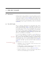
Creating new LRP structure by using the graphics user interface
This method is the preferred method of creating the LRP structure. It is
the simplest and least error-prone approach. To create the structure, run
the graphics user interface (fig. 2.1) by selecting the Start GUI from the
LRP menu, shown as the item in the Scilab main menu. If there are no
structure named lrp, it will be automatically created.

The created structure is named lrp. Any other structure of this name is
deleted. If you need to preserve the old system, assingn it a different name,
e.g. myLrp = lrp;

If you cannot find the LRP menu, close the Scilab and run the Toolkit
again. If it does not work or you do not want to close the Scilab session,
run the install.sci script file by typing
global LRP_OPTIONS ;
cd ( LRP_OPTIONS . path );
exec ( ’ install . sci ’ );
The first two lines set the Toolkit directory. If you have problems with
them, use the cd(PATH_TO_LRP_TOOLKIT), where PATH_TO_LRP_TOOLKIT is
the directory where you installed the LRP Toolkit — if you are unsure about
it, try the contrib/lrp directory in the main Scilab directory.
You will now see the LRP Toolkit user interface, shown on fig. 2.1 To create
a new LRP system, click Create a new system button, positioned in the
upper-left corner of the GUI. This will start the new system creator. You
will need to give the following information:
• the number of states (n), inputs (r) and outputs (m) in the system
• all the system matrices (A, B, B0, C, D, D0)
• the pass length α and the number of passes to simulate β.
2 THE LRP TOOLKIT
9
Figure 2.1: The main Toolkit GUI
To simplify entering the matrix’ values click on the ellipsis button. Alternatively you may use the Scilab functions that return an appropriatelydimensioned matrix.
!
If you use functions, you cannot use the ellipsis button. Moreover you are
responsible for checking the dimensions of matrices.
Standard boundary
conditions
Note that the resulting process will have zero input and standard boundary
conditions
xk+1 (0) = 0, k ≥ 0,
(2.1)
y0 (p) = 1,
You may change them using the Initial conditions button.
To change the pass length and the number of simulated passes click the
Change parameters button.
If any of the values were changed outside the Toolkit GUI, click Update matrices
button to feed the proper values into the GUI.
To close the GUI, click Exit.
2.4.2
Creating new LRP structure by using createLRPModel
This function is especially useful in scripts. This function can be called with
many different arguments. For detailed description type help createLRPModel
in the Scilab window.
To create a sample system use lrp = createLRPModel(); The created system has 2 states, 3 inputs and 4 outputs. The system matrices are random
from 0 to 1. The pass length α = 10 and number of simulated passes β = 15.
The external input u equals zero. To change the boundary conditions, see
section 2.4.4.
2 THE LRP TOOLKIT
2.4.3
10
Creating new LRP structure by using createStubLRP
If you need greater control over the creation process, use the createStubLRP
function to create the necessary fields. Then fill all the stub values with data.
!
!
2.4.4
If you do not fill all the stub values the Toolkit will not function correctly.
To check the correctness of the LRP structure, use the checkLRP function.
Do not forget to set the lrp.controllers field!
Setting the boundary conditions
To set the boundary conditions of the LRP structure named lrp, use the
appropriate generator function:
For state x
• lrp = boundCond_x1(lrp) for xk (0) = 1
• lrp = boundCond_xsin(lrp) for xk (0) of a sine wave of unit height
and a period of one.
• lrp = boundCond_xsin(lrp,T) for xk (0) of a sine wave of unit height
and a period of T.
For output y
• lrp = boundCond_y1(lrp) for y0 (p) = 1
• lrp = boundCond_ysin(lrp) for y0 (p) of a sine wave of unit height
and a period of one.
• lrp = boundCond_ysin(lrp,T) for y0 (p) of a sine wave of unit height
and a period of T.
2.5
Visualization of the process dynamics
The Toolkit can be used to visualise the process dynamics. All the standard
methods of visualisation are available:
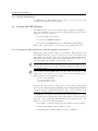
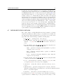
2.5.1
Along the pass plots
This plot is useful for showing the dynamics of the whole pass (along the p
dimension). It is also very important tool for comparing the shape of a few
passes.
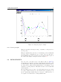
This plot emphasizes the p direction. To draw this plot, the user must first
select the pass k for which the plot is to be made. Upto 32 passes can be
shown simultanously. On the X points p are shown, the value is given on
the Y axis. The example of such plot is shown on figure 2.2.
2 THE LRP TOOLKIT
11
]
Figure 2.2: Along the pass plot example
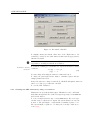
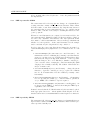
2.5.2
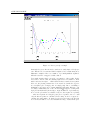
Pass to pass plot
This plot is useful for showing the change of dynamics over all passes for a
selected point p.
This plot emphasizes the k direction. To draw this plot, the user must first
select the point p for which the plot is to be made. Upto 32 points can be
shown simultanously. On the X passes k are shown, the value is given on
the Y axis. The example of such plot is shown on figure 2.3.
2.6
IMPROVEMENTS
Since the release of the first version of the LRP Toolkit (see [HCG+ 06])
a vast number of bugs have been fixed. Currently the new release of the
Toolkit is available. The most important change is that the functions that do
not depend on the considered model structure have been rewritten to accept
a much more general parameters. This makes extension of the Toolkit much
easier in practice.
After the initial release it became obvious that much stronger type checks
are required. This is motivated by a fact that the linear repetitive process
model contains many variables that are error-prone. This has lead to a
development of new functions for dealing with this task.
2 THE LRP TOOLKIT
12
]
Figure 2.3: Pass to pass plot example
Currently the great effort is made towards new, vastly improved help system. This is based on standard Scilab templates, but contains many more
illustrative examples. Moreover a number of potential pitfalls is explained.
All such cases have a suggested, valid solution.
Very much attention has been paid to presentation of the results. In the
new version of the Toolkit, the drawing engine has been rewritten to allow
much easier use in scripts — all the functions have a much clearer syntax.
Moreover, the plotting routines have been extended to handle the degenerate cases (like a plot of single point on a single pass). Due to readibility, a
maximum of 32 passes can be drawn simultaneously using different colors
for clarity. Additionally, due to the extended LATEX support, creating multiple plots is much faster (from O(n) to O(1) calculations of plot surfaces),
moreover the plot surface is calculated only for data required for plotting
— when user requests an ”along the pass” plot for points 7..18 for α = 100
only the first 18 points are calculated. If necessary, it can be requested to
calculate the entire surface. Compared to the previous version, the 3D plots
are now made in full color to better visualize the range of values in the plot.
2 THE LRP TOOLKIT
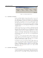
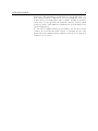
13
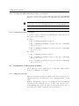
Figure 2.4: Stability analysis window
2.6.1
STABILITY ANALYSIS
In terms of stability analysis for discrete linear repetitive processes of the
form considered here, asymptotic stability (and hence the construction of
the resulting limit profile described by a 1D discrete linear systems state
space model) is simple to check by means of Theorem 1, as it requires that
all eigenvalues of the matrix D0 in (1.1) have modulus strictly less than
unity (this task is much harder for the case when the pass initial condition
is an explicit function of the previous pass profile.) Asymptotic stability
test is implemented in the Toolkit as the stAsymptotic1 test. Its LMI
counterpart of Theorem 2 is also implemented. This function is termed
stAsymptoticLMI1.
Stability along the pass, however, is a much more challenging task in this
respect. In which context, it has been noted in the introduction that a 1D
Nyquist test can be used but it has not proved a suitable basis to undertake
control law design (in contrast to the 1D case). This has led to the use
of LMI based tests (see Theorem 4) which are sufficient but not necessary
but can be executed using computations with constant entry matrices and,
crucially, provide a basis for control law design. To test the stability along
the pass in the Toolkit by means of Theorem 4, the stAlongThePassLMI1
test can be utilised.
In addition to the most important stability definitions (asymptotic and
along the pass), the Toolkit includes the tests for the so-called practical
stability. This notion lies between the asymptotic and along the pass stability. The tests implemented according to Theorems 5 and 6 are available
as stPractical1 and stPracticalLMI1, respectively.
Both stability properties can be investigated using the LMI technique. One
of the reasons of selecting the Scilab as the host platform for the Toolkit
was the excellent LMI solver available for this platform as ”LMITOOL: a
Package for LMI Optimization in Scilab” [NDG]. Note also that provision
is available to easily include existing or newly developed tests by simply
implementing a single Scilab function with no need to change the GUI,
which is shown on fig. 2.4.
2.6.2
CONTROL LAW DESIGN
As outlined in the Background section, the stabilisation of the linear repetive
process is not always easy. In developing new techniques it is beneficial to
compare the newly developed method with the ones already known. One
approach would be to use the LMI tools already available in Scilab and
2 THE LRP TOOLKIT
14
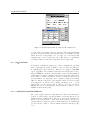
Figure 2.5: Matrix wizard windows: main and the matrix entry
code the methods by hand. However, this approach requires substantial
knowledge about the internal data structures used by the LMI solver and
this is not ideal. Consequently a set of ready-to-use control law design
templates have been incorporated into the toolkit. Moreover, expanding it
by adding additional control law design methods is a simple task.
2.6.3
LATEX EXPORT
Presentation of simulation results can be a time consuming task, especially
when considering large matrices which are often encountered in this area.
To simplify this tedious task the toolkit has been equipped with LATEX
export capabilities. An essential novelty is the fact that the user needs to
write the LATEX file, adding the tags that will be replaced by the simulation
results, instead of using a complicated syntax of the previous Toolkit version.
It is possible to include any number of plots, both 2D and 3D. On each
plot any number of points/passes can be displayed, which is an essential
difference with the ”interactive” plots discussed earlier. Note however that
32 points/passes on each plot can be displayed in unique colors — a great
improvement over the previous version. The process of plot selection is
simplified by the use of an interactive wizard. It is also possible to export
simulation data from the script.
2.6.4
USABILITY ENCHANCEMENTS
One of the design goals was to make this new toolkit as user friendly as
possible. To achieve this, a ”new system wizard” for entering various process
parameters has been implemented. Since most of the model parameters are
matrices, the basic method to define these is the Scilab convention for
entering matrices (exactly the same as in the Matlab). To simplify this
process, it is also possible to enter the matrix element-by-element (see Fig.
2.5).
2 THE LRP TOOLKIT
15
To make the end product available for a broader audience, the Windows operating system version employs an easy to use multilingual (currently Polish
and English) installer based on Nullsoft Install System (NSIS ) [Nul]. This
system is widely regarded to be a very reliable, free solution that produces
a small overhead code. Additionally, the NSIS can package and verify all
the files included into the prepared compilation. Moreover, as an additional
safety measure, for each installed file the Message-Digest Algorithm 5 (better known as MD5) checksum is calculated using the MD5 library [pL]. This
value is used when upgrading and uninstalling the toolkit — if any change
is detected, the user can choose to leave the file intact. Essentially, this
feature provides protection against accidental deletion of manual changes.
During the installation phase, an existing LATEX installation is automatically
detected. Currently, the most popular MiKTeX distribution is supported
by the installer, but any standard LATEX can be used.
2.7
IMPLEMENTATION DETAILS
The toolkit consists of a TCL/TK GUI frontend and a number of Scilab
script files and functions. All the basic process parameters are included in
the lrp structure which is implemented as a new type based on the tlist
(typed list; native Scilab datatype) with the following fields:
• lrp Sys Cla — (string), name of the data type
• The lrp.mat field of type lrp Sys Cla Mat used for storing the model
matrices — see (1.1). Currently it contains the values of A, B, B0, C,
D, D0 —
• The lrp.dim field of type lrp Sys Cla Dim used for storing the model
dimensions. Currently it has the following fields
– alpha — (positive integer), pass length (number of points on
each pass), denoted α in (1.1),
– beta — (positive integer), number of passes over which the
simulation will run,
– n, r, m — (positive integers), dimensions of state, input and
output vectors respectively,
• The lrp.ini field of type lrp Sys Cla Ini used for storing the initial
conditions. Currently it has two fields:
• x0, y0 — (real matrices), boundary conditions, see (2.1). Note that
xk+1 (0) in (2.1) is here denoted by x0 for simplicity,
• controller — (list), list of known control laws for the process; see
below,
• indController — (positive integer), index of current control law.
This field contains the index of currently active control law. If indController=1
then no control law is applied.
• stability — (list), list of performed stability tests; see below.
Note that the model of (1.1) does not impose any constrains on the number
of passes and hence to simulate the process response it is necessary to bound
2 THE LRP TOOLKIT
16
it by some finite value selected by the user — hence the parameter beta in
the lrp structure.
2.7.1
THE lrp.controller FIELD
The controller field of the lrp Sys Cla datatype is a dynamically increasing list that contains a number of tlist structures. Each element
holds the results of control law calculations. By design the first element of
the controller list (i.e lrp.controller(1)) is a copy of all the system
matrices. This ,,controller” is necessary for retaining the matrices for the
open-loop system.
When new control law matrices are computed, a new tlist is added to the
lrp.controller field. This field is defined by the user and the toolkit does
not enforce any constraints on its structure. The only requirement is that
there must be a field solutionExists of the boolean type which informs
whether or not it is possible to obtain control law matrices for the example
under consideration by the design method being considered.
In order to introduce a new control law the user must 1) give it a name (e.g.
controllerExample) and 2) implement a set of 3 functions and one .tex
file:
• controllerExample (the same name as a control law name) — the
main function used for calculating the (constant) control law matrices
given a process state space model. This approach allows faster calculations but also imposes an important drawback — it is not possible
(without changes to the core Toolkit files) to simulate controlled process to asses the effects of varying the control law matrix (K). (LMI
designs produce a family of such K). The addition of this feature is a
subject for future work.
• setcontrollerExample (set+controller name) — change the system
matrices to depict the controlled process (e.g. replace the A matrix
into A + B · K matrix where K is the calculated (constant) control
law matrix).
• writecontrollerExample (write+controller name) — a Scilab function for exporting the results (e.g. controller matrices, parameters
etc.) to LATEX, can be blank if no export is required
• describecontrollerExample.tex (describe+controller name) — introductory text in LATEX to be inserted when using the LATEX export
capabilities, can be left blank.
It must be stressed that the Toolkit files written by the user must be placed
in the appropriate directories — this is explained in the help file. Note also
that the Scilab enforces a maximum function name length of 25 characters.
2.7.2
THE lrp.stability FIELD
The stability field of the lrp Sys Cla datatype is a dynamically increasing list that contains a number of tlist structures. Each element represents a preformed stability test.
2 THE LRP TOOLKIT
17
When the user checks a new stability condition, a new tlist is added to
the lrp.stability field. This field is defined by the programmer and the
toolkit does not enforce any constrains on its structure. The only requirement is that there must be a field solutionExists of integer type (note here
the difference between lrp.stability and lrp.controller field where a
boolean type is used instead) which informs the user whether the system
is stable, unstable or the method used does not provide the answer. The
solutionExists field can have the following values
• −1 - test is inconclusive. In this case the only alternative is to use
another test.
• 0 - the process is unstable,
• 1 - the process is stable.
Obviously the Scilab works in finite precision arithmetic and hence numerical errors can influence the results.
To implement a stability test the programmer should write a function that
returns an lrp structure and is given one as the only argument. Note
here that a better solution would be to use a “by variable” (or by pointer)
passing method but this is not implemented in Scilab. This function must
be placed in the stability directory of the toolkit.
To conserve memory, the lrp.stability field is dynamically created. If
the user does not complete any stability tests then this field does not exist.
2.7.3
THE BOUNDARY CONDITIONS
The boundary conditions of (2.1) can be entered either as a set of values, or
by providing a function that returns the appropriate value given the pass k
and point number p.
By default, if the user does not supply the boundary conditions, they are
assumed as
xk+1 (0) = 0
y0 (p) = 1
2.8
THE COOLMATRIX TYPE
The conducted usability tests have shown that, due to differences in indexing
between the theoretical results and the Scilab requirements, the implementation of any function can very easily lead to the famous ”fencepost” error
— for example, if the user wants to see pass number 3 he has to enter the index 4 in the Scilab matrix. While this problem may seem simple, it can lead
to many difficult-to-detect errors, especially for non-standard LRP systems
(like the ”wave” processes, where negative indices are often used).
To overcome this difficulty, the new version of the Toolkit includes the
CoolM atrix matrix type that allows the user to index the arrays as required
(from 0 or any other value, including negative number). The functions used
for this type are designed for fast prototyping and hence provide a strict
error checking — any attempt to use a wrong index causes an error. Great
effort has been made to make this type compatible with the standard Scilab
2 THE LRP TOOLKIT
18
matrix type. The disadvantage of this addition to the Toolkit is the overhead caused by this type. This fact does not very significant, as the type
is aimed at the prototyping phase, where a small to medium problems are
tested. Moreover, the experience shows that the efficiency of the Toolkit is
greatly dependent on the LMI solver, which has the greatest impact in the
practical applications.
To create the CoolMatrix variable, the user must provide the allowed range
of indices. Note here that the Scilab notation of ”extending” the size of the
matrix when called with index larger than its former size is not supported,
as this is very error-prone.
3
Example
To illustrate the LRP Toolkit, consider the special case of (1.1) defined by
the following matrices


 


0.19 0.07 0.19
0.8
0.1 0.2
A = 0.02 0.85 0.49 , B = 0.7 , B0 = 0.3 0.1 ,
0.84 0.01 0.75
0.3
0.6 0.2
0.5 0.3 0.1
0.2
0.44 0.26
C=
,D =
, D0 =
.
0.2 0.4 0.1
0.4
0.08 0.07
with pass length α = 10 and boundary conditions
y0 (p) =
xk (0) =
sin(p)
0.9
sin(p)
0.9
0.9
T
for
T
for k ≥ 0.
0 ≤ p < α,
(Note that the argument of the sin function is given in radians).
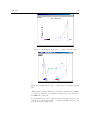
By using the stability analysis options offered by the toolkit we conclude
that the process is asymptotically stable but unstable along the pass. The
plots of the pass profiles for k = 3, 5, 7, 12, 15, 20 confirm this (note the
amplitudes of pass profile vectors increase significantly (see Fig. 3.1) as the
process dynamics evolve).
Suppose now that the task is to design a control law of the form (1.6) to
ensure stability along the pass. This can be undertaken using the toolkit stabilizing control law design options, as detailed in Section 2.6.2. For demonstration purposes we consider the case (in actual fact the theory behind this
design produces a family of possible choices for K) when the control law
matrix K of (1.6) is given by
K = −0.4887 −0.5174 −0.6102 −0.4543 −0.2739 .
Note here that the user does not have to execute any commands to compute
the resulting controlled process state space model — this is automatically
done. The resulting controlled stable along the pass process state space
model is of the form (1.1) with


 
−0.201 −0.3439 −0.2982
0.8
A = −0.3221 0.4878 0.06287  , B = 0.7 ,
0.6934 −0.1452 0.5669
0.3


−0.2634 −0.01911
0.3491 0.2052
B0 = −0.01802 −0.09172 , D0 =
,
−0.1017 −0.03956
0.4637
0.1178
0.4023 0.1965 −0.02204
0.2
C=
,D =
.
0.004519 0.193 −0.1441
0.4
3 Example
20
Figure 3.1: Instability along the pass — output 1 along the pass
Figure 3.2: Stability along the pass — controlled process output 1 along the
pass
All the matrices obtained during the control law computations are available
to the user by using the options supplied and they can be also exported to
the LATEX-based source file.
A representative plot of the evolution of the pass profile sequence for the
controlled process is given in Fig. 3.1 and the stability along the pass
property is evident by inspection.
3 Example
3.1
21
CONCLUSIONS AND FUTURE WORK
The Scilab toolkit whose development has been described in this paper has
already been useful in the analysis and control law design for discrete linear
repetitive processes of the form considered here. Its basic functions include
the simulation engine and the stability analysis/control law design abilities.
A key point to note is that this toolkit removes the limitations present in
others. Moreover, the user is able to export the results to the valid LATEX
compatible format text file.
Software development for this toolkit is an ongoing process; there are many
options which remain to be implemented. A representative sample of on
going development work is the following topics:
• support for new classes of processes (such as ”wave” or semi-linear)
and for a differential process model where the dynamics along the pass
are governed by a linear matrix differential equation couple along with
discretization methods,
• addition new control law design algorithms,
• control law design for stability and performance (e.g. ensuring that a
reference signal is tracked, minimization of the influence of the external
disturbances),
• handling of processes with uncertainty in the state space model,
• an installer for the Linux/Unix version.
Results from this work will be reported in due course.
4
4.1
Appendix
Abbreviations and notation
Throughout the manual the following abbreviations and notations are used
Notation
GUI
LRP
≺
r(M )
Meaning
Graphics user interface
Linear Repetitive Process or
type of a structure used by the Toolkit to represent such process
positive definitiveness of a matrix
negative definiteness of a matrix
the spectral radius, the largest module of an eigenvalue of matrix M
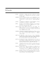
Bibliography
[Ben00]
S. E. Benton. Analysis and Control of Functions of Linear
Repetitive Processes. PhD Dissertation, University of Southampton, UK., 2000.
[BGFB94] S. Boyd, L. E. Ghaoui, E. Feron, and V. Balakrishnan. Linear
Matrix Inequalities In System And Control Theory, volume 15
of SIAM studies in applied mathematics. SIAM, Philadelphia,
1994.
[CCN06]
S.L. Campbell, J.P. Chancelier, and R. Nikoukhah. Modeling
and Simulation in Scilab/Scicos. Springer, 2006.
[DD03]
R. D’Andrea and G. E. Dullerud. Distributed control design for
spatially interconnected systems. IEEE Transactions on Automatic Control, 48(1):1478–1495, 2003.
[GDB+ 98] Claude Gomez, Francois Delebecque, Carey Bunks, JeanPhilippe Chancelier, Serge Steer, and Ramine Nikoukhah, editors. Engineering and Scientific Computing with Scilab with
Cdrom. Birkhauser Boston, 1998.
[GGGR05] J. Gramacki, A. Gramacki, K. Galkowski, and E. Rogers. Java
based toolbox for linear repetitive processes. Proc. 2nd Int.
Conf. on Inform. in Control, Autom. and Robotics — ICINCO,
1:182–187, 2005.
[GLR+ 03] K. Galkowski, J. Lam, E. Rogers, S. Xu, B. Sulikowski,
W. Paszke, and D. H. Owens. Lmi based stability analysis and
robust controller design for discrete linear repetitive processes.
Int. J. Robust Nonlinear Control, 13:1195–1211, 2003.
[GPS+ 03] K. Galkowski, W. Paszke, B. Sulikowski, E. Rogers, and D. H.
Owens. LMI based stability analysis and robust controller design
for discrete linear repetitive processes. International Journal of
Robust and Nonlinear Control, 13(13):1195–1211, 2003.
[Gra99]
J. Gramacki. Metody badania stabilności i stabilizacja liniowych,
dyskretnych procesow powtarzalnych. PhD thesis, Politechnika
Zielonogorska, 1999.
[HCG+ 06] L. Hladowski, B. Cichy, K. Galkowski, B. Sulikowski, and
E. Rogers. Scilab compatible software for analysis and control
of repetitive processes. Proc. IEEE International Symposium on
Computer-Aided Control Systems Design, CACSD 2006, 2006.
[MCA03]
H. Melkote, B. Cloke, and V. Agarwal. Modeling and compensator designs for self-servowriting in disk drives. Proc. American
Control Conference, 1:737–742, jun 4-6 2003.
Bibliography
24
[NDG]
R. Nikoukhah, F. Delebecque, and L. E. Ghaoui. LMITOOL: a
package for LMI optimization in scilab.
[Nul]
Nullsoft. Nsis users manual.
[OARF00] D. H. Owens, N. Amann, E. Rogers, and M. French. Analysis of
linear iterative learning control schemes - a 2D systems/repetitive processes approach. Multidimensional Systems and Signal
Processing, 11(1-2):125–177, 2000.
[pL]
Matthew ”IGx89” Lieder. Md5 plugin dll.
[RHL+ 05] J. D. Ratcliffe, J. J. Hatonen, P. L. Lewin, E. Rogers, T. J.
Harte, and D. H. Owens. P-type iterative learning control for
systems that contain resonance. International Journal of Adaptive Control and Signal Processing, 19(10):769–796, 2005.
[RO92]
E. Rogers and D. H. Owens. Stability Analysis for Linear Repetitive Processes, volume 175 of Lecture Notes in Control and Information Sciences. Springer-Verlag, 1992.
[SG]
INRIA Meta2 Project/ENPC Cergrene Scilab Group. Introduction to scilab.
[SGRO05] B. Sulikowski, K. Galkowski, E. Rogers, and D. H. Owens.
Control and disturbance rejection for discrete linear repetitive
processes. Multidimensional Systems and Signal Processing,
16(2):199–216, 2005.
[Sul06]
B. Sulikowski. Computational aspects in analysis and synthesis
of repetitive processes. PhD thesis, University of Zielona Gora,
2006.
Index
Index
ILC, see Iterative Learning Control
Iterative Learning Control, 1
Linear Repetitive Process, 1
Boundary conditions, 2
Model, 1
Stability, 2
Along the pass, 2
Asymptotic, 2
Linear Repetitive process
Applications, 1
Repetitive processes, 1
Standard boundary conditions, 9
25