Download High Level Reduction Technique for Multiway Decision

High Level Reduction Technique for
Multiway Decision Graphs Based Model
Checking
Ghiath Al Sammane, Sa’ed Abed and Otmane Ait Mohamed
Department of Electrical and Computer Engineering
Concordia University
1455 de Maisonneuve
Montreal, Quebec, H3G 1M8, Canada
{sammane, s abed, ait}@ece.concordia.ca
Abstract
Multiway Decision Graphs (MDGs) represent and manipulate a subset of first-order
logic formulae suitable for model checking of large data path circuits. Due to the
presence of abstract variables, existing reduction algorithms that is defined on
symbolic model checking with BDD cannot be used with MDG. In this paper we
propose a technique to construct a reduced MDG model for circuits described
at algorithmic level in VHDL. The simplified model can be obtained using a high
level symbolic simulator called TheoSim, and by running an appropriate symbolic
simulation patterns. Then, the actual proof of a temporal MDG formula will be
generated. We support our reduction technique by experimental results executed on
benchmark properties.
Keywords: Model-checking , Symbolic Simulation, Behavioral Models
1. INTRODUCTION
The current context of systems-on-a-chip design involves the use of large architectural blocks,
such as CPU cores, complex operators, and parameterized memory modules. These components
are typically specified with algorithms written in high level languages like C++ and Matlab, and
their behavioral description extensively validated, mainly by the simulation of test cases.
At this stage, theorem-proving techniques are gaining attention, but their use is still considered
difficult and time consuming. Model checking stills the automatic formal verification technique
that is preferred for industrial flows. It aims by exploring the reachable state space of a model to
verify that an implementation satisfies a specification [1]. Binary Decision Diagram (BDD) [2] is
the canonical representation for Boolean functions that is used initially by model checker as an
efficient encoding for the state space at the Boolean level.
In fact, efficient equivalence checking tools are available at the the Register Transfer Level
(RTL) and below. New, property checking of logic-level control parts is gaining steam, with the
combination of BDD’s, Satisfiability (SAT) solvers, and simulation. In order to use these existing
tools and methods directly on system level models a synthesis step is needed. Then, the space
state becomes, in most cases, extremely large and that leads to the problem of state-explosion,
which limits the applications of to small-to-medium systems.
Multiway Decision Graphs (MDGs) [3] is an alternative that extended BDD and SAT based model
checking. MDG represents and manipulate a subset of first-order logic formulae suitable for
large system level circuits. With MDGs, a data value is represented by a single variable of an
abstract type and operations on data are represented in terms of an uninterpreted functions.
The MDG operations and verification procedures are packaged as MDG tools and implemented
High Level Reduction Technique for MDG Based Model Checking
in Prolog [5] providing facilities for invariant checking, verification of combinational circuits,
equivalence checking of two state machines and model checking.
Due to the presence of abstract variables, existing reduction algorithms which are defined on
symbolic model checking with BDD cannot be used with MDG. In this paper we propose a simple
but powerful technique to construct a reduced MDG model for circuits described at algorithmic
level in VHDL. By using a high level symbolic simulator called TheoSim, and by running an
appropriate symbolic simulation patterns before the actual proof of a temporal MDG formula,
an important model simplification can be obtained. We support our reduction technique by
experimental results executed on benchmark properties.
The organization of this paper is as follows: Section 2 gives some preliminaries on MDG system
and TheoSim, respectively. The main contribution of the paper describing the reduction technique
is presented in Section 3. Section 4 discusses experimental results of applying our reduction
methodology. Section 5 and 6, review the related work in the area and discuss the possibilities for
future research directions, respectively.
2. PRELIMINARIES
2.1. The Multiway Decision Graph
Multiway Decision Graph (MDG) is a graph representation of a class of quantifier-free and
negation-free first-order many sorted formulas, called Directed Formulae, (DFs) [3]. DFs can
represent the transition and output relations of a state of machine, as well as the set of states.
As in ordinary many-sorted First Order Logic (FOL), terms are made out of sorts, constants,
variables, and function symbols. Two kinds of sorts are distinguished: concrete and abstract:
• Concrete sort is equipped with finite enumerations, lists of individual constants. Concrete
sorts is used to represent control signals.
• Abstract sort has no enumeration available. It uses first order terms to represent data
signals.
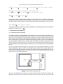
Figure 1 shows two examples G0 and G1. In G0, x is a variable of the concrete sort [0, 1, 2, 3]. By
contrast, in G1 x is a variable of abstract sort where α, β and f (θ) are abstract terms.
'ϭ
'Ϭ
ŽŶĐƌĞƚĞǀĂƌŝĂďůĞ
Ϭ
'͛
ďƐƚƌĂĐƚǀĂƌŝĂďůĞ
X
Ϯ
'͛
ϯ
X
α
f (θ)
β
'͛͛
'͛
'͛
'͛͛
FIGURE 1: Example of Multiway Decision Graphs Structure
MDG terms are well formed first-order term. Let F be a set of function symbol and V a set of
variables. We denote the set of terms freely generated from F and V by T (F, V). The syntax
of a Directed formulae DF is then given by the grammar below [4]. The underline is used to
High Level Reduction Technique for MDG Based Model Checking
differentiate between the concrete and abstract.
Sort S
Abstract Sort S
Concrete Sort S
Generic Constant C
Concrete Constant C
Variable X
Abstract Variable V
Concrete Variable V
Directed Formulae DF
Disj
Conj
Eq
::=
::=
::=
::=
::=
::=
::=
::=
::=
::=
::=
::=
S | S
α | β | γ | ···
α | β | γ | ···
a | b | c | ···
a | b | c | ···
V | V
x | y | z | ···
x | y | z | ···
Disj
| > | ⊥
Conj ∨ Disj | Conj
Eq ∧ Conj | Eq
A = C (A ∈ T (F, V ))
|V =C
| V = A (A ∈ T (F, X ))
Directed Formulae are always disjunction of conjunctions of equations or True or False (terminal
case). The Disj can be disjunction of conjuncts or a conjunct only. Also, the conjunction Conj is
defined to be an equation only Eq or a conjunction of at least two equations. Atomic formulae are
the equations, generated by the clause Eq. The equation can be the equality of concrete term
and an individual constant, the equality of a concrete variable and an individual constant, or the
equality of an abstract variable and an abstract term.
Directed Formulae are used for two purposes: to represent sets (viz. sets of states as well as
sets of input vectors and output vectors) and to represent relations (viz. the transition and output
relations).
2.2. The MDG-Tool
The MDG operations and verification procedures are packaged as MDG tools and implemented
in Prolog [5]. The MDG tools provide facilities for invariant checking, verification of combinational
circuits, sequential verification, equivalence checking of two state machines and model checking.
It is based on a limited nesting of temporal operators (other than X) where existential abstraction
and a Prune-by-Subsumption are applied to compute a merged set of reachable states.
The input language of the MDG tool is a Prolog-style hardware description language (MDGHDL) [6], which supports structural specification, behavioral specification or a mixture of both. A
structural specification is usually a netlist of components connected by signals, and a behavioral
specification is given by a tabular representation of transition/output relations or a truth table.
In MDG model checking, the system is expressed as an Abstract State Machines (ASM) and
the properties to be verified are expressed by formulas in LM DG . LM DG atomic formulas are
Boolean constants (True and False), or equations of the form t1 = t2 , where t1 is an ASM variable
(input, output or state variable) and t2 is either an ASM system variable, an individual constant, an
ordinary variable or a function of ordinary variables. Ordinary variables are defined to memorize
the values of the system variables in the current state.
Any LM DG formula is built using the basic operator N ext let f ormulae, in which only the temporal
operator X (next time) is allowed. The structure of N ext let f ormulae is defined as follows (see
[4] for more details):
• Each atomic formula is a N ext let f ormulae;
• If p, q are atomic formula then the following are N ext let f ormulas:
– !p (not p), p&q (p and q) p|q (p or q), p → q (p implies q)
– Xp (next-time p)
– LET (v=t) IN p, where t is a system variable and v an ordinary variable.
High Level Reduction Technique for MDG Based Model Checking
Model checking of a property p in LM DG on an ASM M is carried out by building ASMs
for sub-formulae containing only the temporal operator X. Then, these additional ASMs are
composed with M . Thus, a simpler property is checked on the composite machine [7].
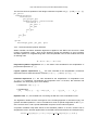
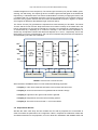
Figure 2 shows the structure of the MDG-tool. In order to verify designs with the tool, we first need
to specify the design in MDG-HDL (design specification and design implementation). Moreover,
an algebraic specification is to be given to declare sorts, function types, and generic constants that
are used in the MDG-HDL description. Rewrite rules that are needed to interpret function symbols
should be provided here as well. Like for ROBDDs, a symbol order according to which the MDG is
built should be provided by the user. However, there are some requirements on the node ordering
of abstract variables and cross-operators (but not for concrete variables). This symbol order can
affect critically the size of the generated MDG. Otherwise, MDG uses automatic dynamic ordering.
WƌŽƉĞƌƚLJ
^ƉĞĐŝĨŝĐĂƚŝŽŶ
ĞŚĂǀŝŽƌĂů
DŽĚĞů
ůŐĞďƌĂŝĐ
^ƉĞĐŝĨŝĐĂƚŝŽŶ
sĂƌŝĂďůĞƐ
KƌĚĞƌ
D'ŽŶƐƚƌƵĐƚŝŽŶ
^ƚƌƵĐƚƵƌĂů
DŽĚĞů
DŽĚĞůŚĞĐŬŝŶŐ
ƋƵŝǀĂůĞŶĐĞŚĞĐŬŝŶŐ
/ŶǀĂƌŝĂŶƚŚĞĐŬŝŶŐ
zĞƐͬEŽ;ŽƵŶƚĞƌĞdžĂŵƉůĞͿ
FIGURE 2: The Structure of the MDG-tool
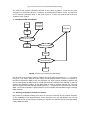
2.3. TheoSim
TheoSim is a high level symbolic simulator based on the System of Recurrence Equations (SRE)
model and implemented in the Computer Algebra System Mathematica [10]. It makes use of
Mathematica symbolic engine and its built-in algebraic simplification rules.
QVLPXODWLRQ F\FOHV
9+'/
)LOH
65(
([WUDFWLRQ
7KHPRGHO
65(
6\PEROLF
WHVWFDVHV
(YHQWEDVHG6\PEROLF
6LPXODWRU
5HVXOWV
6LPXODWLRQ
5XOHV
FIGURE 3: Overview of TheoSim
As shown in Figure 3, TheoSim provide a compiler that extracts automatically the SRE model
from a VHDL behavioral design, an automatic generator of simulation patterns, and an event
driven symbolic simulator written in Mathematica
High Level Reduction Technique for MDG Based Model Checking
2.3.1. The System of Recurrence Equations (SRE)
A System of Recurrence Equations (SRE) is a 5-tuple :
SRE =< Inputs, S, DomainsInputs∪S , T F >
• All the elements in Inputs and in S are represented as time variables of the form Xi (n).
• Inputs = {I1 (t), I2 (t), . . . , In (t)} is the set of input signals of the system
• S = Locals ∪ Outputs = {S1 (t), S2 (t), . . . , Sm (t)}, is the set of simulated objects. With:
– Locals is the set of internal signal and variables
– Outputs is the set of output signals of the system
• DomainInputs∪S is the set that contains the mathematical domain of each element in Inputs
and S.
• T F is the transition function that describes the behavior of the system at the end of
simulation cycle t; written as set of recurrence equations, one equation for each elements in
S: For a circuit that contains m objects (signals + variables), we extract automatically a set
of m Equations: {Xi (t)}0<i≤m where, Xi (t) is the value of the object i at time t given as a
recurrence equation:
Xi (t) = fi (Xj (t − γ))
with m, i, j, γ ∈ N, and (0 < i ≤ m, 0 < j ≤ m, 0 < γ), ∀t ∈ N
These equations form an algebraic partitioned version for the transition relation of the circuit. It is
analyzed using a cone of influence based algorithm [9], which means that all variables that do
not influence the value of the object Xi (t) are eliminated from the expression of the function f .
The function f is normalized using a generalized if-then-else expressions.
For example, considering the behavioral counter described in VHDL:
entity counter
port(clock:
clear:
count:
q
:
);
end counter;
is
in bit;
in bit;
in bit;
out integer
architecture behv of counter is
signal pre_q: integer;
begin
process(clock)
begin
if clear = ’1’ then
pre_q <= pre_q - pre_q;
elsif (clock=’1’ and clock’event) then
if count = ’1’ then
pre_q <= pre_q + 1;
end if;
end if;
end process;
q <= pre_q;
end behv;
The SRE of this counter is :
Inputs = {clock(t), clear(t), count(t)},
Locals = {pre q(t)},
Outputs = {q(t)},
DomainsInputs∪S = {clock(t) ∈ B, clear(t) ∈ B, count(t) ∈ B, pre q(t) ∈ Z, q(t) ∈ Z}
High Level Reduction Technique for MDG Based Model Checking
The set of recurrence equations of the design contains the equation of (q(t + 1) and pre q(t + 1)):
pre_q(t+1)=
IF(Event(clock(t))
,IF(clear(t)=1
,pre_q(t)-pre_q(t)
,IF(And(clock(t)=1, event(clock(t)))
,IF(count(t) = 1
,pre_q(t)+ 1
,pre_q(t)
)
,pre_q(t)
)
)
,pre_q(t)
)
,q(t+1)=
IF(event(pre_q(t)), pre_q(t), q(t) )
2.3.2. The Event Based Symbolic Simulator
Within TheoSim, the VHDL simulation algorithm is applied on the SRE of the circuit for a fixed
number of simulation cycles n given by the designer. During the simulation, a set of symbolic
simulation patterns ∆ is applied along with a set of simplification rules R that contains four kinds
of rewriting rules:
R = RM ath ∪ RLogic ∪ RIF ∪ REq
Polynomial symbolic expressions RM ath : are built-in rules intended for the simplification of
polynomial expressions (Rn [x]).
Logical symbolic expressions RLogic : are rules intended for the simplification of Boolean
expressions and to eliminate obvious ones like (and(a, a) → a) and (not(not(a)) → a).
If-formula expressions RIF : are rules intended for the simplification of computations over
if-then-else expression. The definition and properties of the IF function, like reduction and
distribution, are used (see [11] for more details):
• IF Reduction: IF (x, y, y) → y
• IF Distribution:
f (A1 , . . . , IF (x, y, z), . . . , An ) → IF (x, f (A1 , . . . , y, . . . , An ), f (A1 , . . . , z, . . . , An ))
Equation rules: REq are resulted from converting an SRE into a set of substitution rules.
The algorithmic details and the convergence of the rewriting algorithm is discussed in [8]. The
symbolic simulation patterns ∆ can be considered as a set of special assignment for the Inputs
of the circuit at each t and a special initialization sequence for the internal registers.
A symbolic simulation step takes values of the simulation patterns ∆ at time t and the set of
simplification rules R and then applies them on the SRE until the achievement of a fixed point (FP).
SymSim Step({Xi (t)}0<i≤m , ∆, t) = Replace U ntil F P ({Xi (t)}0<i≤m , R, ∆, t)
High Level Reduction Technique for MDG Based Model Checking
The result of the symbolic simulation depends on the nature of patterns ∆ that can vary from
a sequence of numerical values to a sequence of uninterpreted functions. In fact, the efficiency
of our reduction technique relies on the good choice of ∆ which can reduces the recurrence
equations of the system.
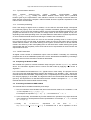
3. THE REDUCTION TECHNIQUE
Symbolic
Simulation
Patterns
VHDL
Properties
SRE
Symbolic Simulation
Reduced
SRE
Models Composition
MDG
Model Checking
Results
FIGURE 4: Overview of the Reduction Methodology
We start with a circuit design written in VHDL and a set of properties written in LM DG . As shown
in Figure 4, we extract form the VHDL design a mathematical model in terms of a System of
Recurrence Equations (SRE). From the properties, we write symbolic simulation patterns that
are input along with the SRE model to a high level symbolic simulator. The reduction is done by
applying the simulation patterns on the SRE model in order to obtain a reduced one. The next
step, we compose the reduced SRE model with the LM DG properties and we extract the reduced
MDG. The formal verification is performed then on this resulted reduced MDG using the existing
MDG package.
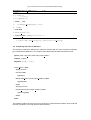
3.1. Defining the Symbolic Simulation Patterns
We provide a systematic strategy that does not need any expertise in the symbolic simulator
or any knowledge of the implementation under verification. Only the specification of the circuit
(expresses as a set of properties) is needed. Our reduction is inspired from [12] but we generalize
it using SRE and MDG.
High Level Reduction Technique for MDG Based Model Checking
3.1.1. Synchronization detection
Some
complex
System-on-Chip
contain
multiple
synchronization
clocks
Clock1 , Clock2 , . . . , Clockm . Usually, the relation between these clocks has a periodical
behavior given by the specifications. One reduction scenario is to assign numerical values for
these internal clocks and to compute a reduced model where the symbolic expressions of the
internal clocks are eliminated.
3.1.2. Functional partitioning
Even if the design of digital circuit is modular, it is rare that the structural design corresponds
to a particular property. Thus, we cannot apply a modular verification approach. Using symbolic
simulation, we can prune the transition relation using functional specifications depending on the
property that we want to verify. The idea is to assign values to the control signals, one by one,
depending on the tested operating mode. The result will be the elimination of symbolic expressions
of non activated functional blocks and reducing the model to the activated one.
However, this assignment freeze the circuit in the selected operating mode. In order to prove
the correctness of the circuit under all operation modes we need to split cases and to compute
several reduced models. The model checking of the system, should be done on all the reduced
models. The efficiency of this case splitting relies on the fact that the model checking time grows
exponentially with the complexity of the circuit and the sum of exponentials is much less than the
exponential of the sum.
3.1.3. RESET elimination
All digital circuits contain an initialization inputs noted as RESET. Practically, the interesting
properties are not in the initialization phase of the circuit. We eliminate the RESET by activating it
for a finite amount of time and then it should be deactivated.
3.2. Computing the Reduced SRE
We simulate the system for several simulation steps using the function SymSim Step defined
above. The simulation algorithm aims to reduce the SRE model by applying ∆ as shown in
Algorithm 1.
Line 1 first initialize the simulation time t to t0 (equal to zero in most cases). The purpose of line 2
and 3 is to store the initial SRE before applying the algorithm. The variables φ and ϕ denote the
reduced SRE and the initial SRE, respectively. Lines 4-7 repeatedly execute a symbolic simulation
for k steps by applying ∆ at the SRE. The algorithm returns the reduced SRE and the initial SRE
(line 8-9). This equivalent to a new SRE where the time variable is changed to T = t0 + k. This
reduced SRE will be used for MDG model-checking.
3.3. Translating the Reduced SRE to MDG
The reduced SRE is translated to MDG by three steps:
1. First, we introduce extra variables that will encode the time instance of a variables Xi and
Xj in the equation Xi (t) = fi (Xj (t − γ)).
For example, the equation X(t) = X(t − 1) + 1 is encoded as X 0 = X + 1.
2. In the second step, we translate any function between the operators in the right hand side
of the equation to uninterpreted functions representation. For example, X 0 = X + 1 become
X 0 = P lus(X, 1).
3. Finally,
an
if-then-else
expression
of
the
form
X
=
IF (condition, then branch, else branch) is translated into a set of equalities of form:
High Level Reduction Technique for MDG Based Model Checking
Algorithm 1 R EDUCE SRE({Xi (t)}0<i≤m , K , ∆)
1: t = t0 ;
2:
ϕ = {Xi (t0 )}0<i≤m ;
3:
φ = {Xi (t0 )}0<i≤m ;
4:
while t ≤ k do
5:
φ = SymSim Step({Xi (t)}0<i≤m , ∆, t)
6:
t = t+1
7:
end while
8:
Reduced InitReg = ϕ;
9:
Reduced SRE = {Xi (T )}0<i≤m / T = t0 + k
(condition ∧ (X = then branch)) ∨ (¬condition ∧ (X = else branch)).
3.4. Comparing with Cone of Influence
The reduction obtained is different from reduction obtained with the cone of influence algorithm
[9]. To illustrate this difference, we consider a basic RAM element defined at behavior level:
Inputs:{reset, chip select, add, data, output enable }
Outputs: {output}
Registers: {reg[0] . . . reg[n]}
if chip select=1 then
Writing Process
if reset=1 then
reg[add]=0
else if (read write=1) and (output enable=0) then
reg[add]=data
end if
Reading Process
if (read write=0) and (output enable=1) then
(output=reg[add])
end if
end if
The transition relation for that circuit is the conjunction of both transition relations of the read and
the write operations, in DF that will be written as follows:
High Level Reduction Technique for MDG Based Model Checking
Read T rDF = (chip select = 1) ∧ (read write = 0) ∧ (output enable = 1) ∧ (output = reg[add])
W rite T rDF = (chip select = 1) ∧ ((reset = 1) ∧ (reg[add] = 0) ∨
(reset = 0) ∧ (read write = 1) ∧ (output enable = 0) ∧ (reg[add] = data))
RAM T rDF = Read T rDF ∧ W rite T rDF
If we want to verify a property about reading on the memory, then it is useful to symbolically
simulate the system with select function assigned to the read active, which eliminates the symbolic
expression of the selection function from the symbolic expression of the property. Thus, we obtain:
Reduced(RAM T rDF ) = (output = reg[add])
The transition relation consists of one clause compared to 4 clauses given by the cone of influence
algorithm (as it will return Read T r).
4. APPLICATION AND RESULTS
4.1. The Island Tunnel Controller
The MDG tool has been demonstrated on the example of the Island Tunnel Controller in [13],
which was originally introduced by Fisler and Johnson [14]. The ITC controls the traffic lights at
both ends of a tunnel based on the information collected by sensors installed at both ends of the
tunnel: there is one lane tunnel connecting the mainland to an island. At each end of the tunnel,
there is a traffic light. There are four sensors for detecting the presence of cars. It is assumed that
all cars are finite in length, that no car gets stuck in the tunnel, that cars do not exit the tunnel
before entering the tunnel, that cars do not leave the tunnel entrance without traveling through the
tunnel, and that there is sufficient distance between two cars such that the sensors can distinguish
the cars.
The ITC controller for the traffic lights at a one lane tunnel connecting the mainland to a small
island as depicted in Figure 5. There is a traffic light at each end of the tunnel; there are also four
sensors for detecting the presence of vehicles: one at tunnel entrance on the island side (ie), one
at tunnel exit on the island side (ix), one at tunnel entrance on the mainland side (me), and one
at tunnel exit on the mainland side (mx).
ŵŐů
ŵƌů
/ƐůĂŶĚ
ŝdž
ŝĞ
ŵdž
ŵĞ
dƵŶŶĞů
ŝƌů
DĂŝŶůĂŶĚ
ŝŐů
FIGURE 5: Island Tunnel Controller Structure
The ITC is composed of five modules: The Island Light Controller, the Tunnel Controller, the
Mainland Light Controller, the Island Counter and the Tunnel Counter (refer to [14] for the state
High Level Reduction Technique for MDG Based Model Checking
transition diagrams of each component). The Island Light Controller (ILC) has four states: green,
entering, red and exiting. The outputs igl and irl control the green and red lights on the island side
respectively; iu indicates that the cars from the island side are currently occupying the tunnel, and
ir indicates that ILC is requesting the tunnel. The input iy requests the ILC to release control of
the tunnel, and ig grants control of the tunnel from the island side as shown in Figure 6. A similar
set of signals is defined for the Mainland Light Controller (MLC).
The Tunnel Counter (TC) processes the requests for access issued by ILC and MLC. The Island
Counter and the Tunnel Counter keep track of the car’s number currently on the island and in the
tunnel, respectively. For the tunnel controller, the counter tc is increased by 1 depending on tc+
or decremented by 1 depending on tc- unless it is already 0. The Island Counter operates in a
similar way, except that increment and decrement depend on ic+ and ic-, respectively: one for the
island lights, one for the mainland lights, and one tunnel controller that processes the requests for
access issued by the other two controllers.
ŵƌů
ŝƵ
ŵƵ
ŵŐů
ŵƌ
DĂŝŶůĂŶĚ
>ŝŐŚƚ
ŽŶƚƌŽůůĞƌ
ŵĞ
ŵŐ
D>
ŵdž
ŝĐ
ŝĐͲ
/ƐůĂŶĚŽŶƚƌŽůůĞƌ
ŝŐ
d
ŵLJ
ŝĐн
ŝƌ
dƵŶŶĞů
ŽŶƚƌŽůůĞƌ
ƚĐ
ŝƌů
/ƐůĂŶĚ
>ŝŐŚƚ
ŽŶƚƌŽůůĞƌ
ŝLJ
ƚĐн
/>
ŝŐů
ŝĞ
ŝdž
ƚĐͲ ŵƚĐн ŵƚĐͲ
dƵŶŶĞůŽŶƚƌŽůůĞƌ
FIGURE 6: Island Tunnel Controller Structure
We would like to establish that the ITC has at least the following properties:
• Property 1: Cars never travel both directions in the tunnel at the same time.
• Property 2: Access to the tunnel is not granted until the tunnel is empty.
• Property 3: Lights don’t turn green until access is granted.
• Property 4: Requests for the tunnel are eventually granted.
• Property 5: There are never more than m cars on the island.
4.2. Experimental Results
We take the same case study and we consider the ITC with its properties as a benchmark in
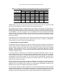
order to measure the performance of our approach. Table 1 compares the verification results with
and without reduction for five properties, run on an Ultra2 Sun workstation with 296MHz CPU and
High Level Reduction Technique for MDG Based Model Checking
TABLE 1: Comparing
Benchmark
Properties
Model Checking Results with & without Reduction
Without Reduction
Time Memory Nodes
With Reduction
Time Memory Nodes
P1
P2
P3
P4
P5
87.41
87.41
87.56
88.77
89.87
45.5
0.56
48.7
48.8
47.5
123080
263
123085
123082
123080
86.99
1.12
14.46
1.02
1.15
43.4
0.4
6.82
0.06
0.58
121060
211
12292
16
241
Average
88.2
38.22
98518
20.95
10,25
26764
768MB memory. We give the CPU time measured in seconds and the memory measured in MB
that are used in building the reduced machine and checking the property.
We remark that the reduction is influenced by the properties. The best gain in performance is
obtained with property P4 where the time is reduced by 77 times the original one and the memory
is reduced by a factor of 88 times. The worst case is the property P1 where the reduction algorithm
is not profitable. In the case of property P1 the assumptions and the functionality tested needs
several runs (when using case splitting). The sum of these runs is equal for this particular case to
a single run without reduction. For P4, it was the other extremum where case splitting was really
much more efficient.
These differences show the sensitivity of the reduction technique to the property verified. Despite
these fluctuations, the average of the gain in performance is a factor of 4 which is considered as
a good result in the case of model checking approaches.
5. RELATED WORK AND DISCUSSION
Compositional model checking [15] is a reduction strategy that aims at splitting a proof goal into
several simple sub-goals, which are determined by choosing appropriate constrain functions for a
subset of primary inputs of the design. From a behavioral point of view, this amounts to applying
Algorithm 1 with parameter k set to 1. The reduced model is constructed according to the user
supplied constrained functions. The strategy we propose generalizes case splitting to a sequence
of values of arbitrary length.
In the same direction, Hazelhurst et al. presented in [16] a hybrid approach relying on the use
of two industrial tools, one for symbolic trajectory evaluation (STE) [17] and one for symbolic
model-checking. STE performs user-supplied initialization sequences and produces a parametric
representation of the reached states set. The result must be systematically converted into a
characteristic function form, before it can be fed to the model-checker. The conversion process is
expensive in the general case [16].
In [12], a model checking reduction by symbolic simulation is presented. This method has been
implemented within the SMV model checker. By contrast to our technique these methods are
applicable only at the Boolean level. However, our methodology is applicable at higher level of
abstraction as it makes use of SRE based symbolic simulation.
In [18] an MDG reduction technique is proposed. A reduced abstract transition system is derived
from the original ASM using only the transition relations of the so-called property dependent state
variables VP of a property P; to be verified. This reduction technique is equivalent only to a cone
of influence reduction. We propose further reductions that includes cone of influence as well.
High Level Reduction Technique for MDG Based Model Checking
6. CONCLUSION AND FUTURE WORK
We have proposed a reduction technique for MDG model checking that uses a high level symbolic
simulation. The symbolic simulation provides behavioral VHDL as an input language for MDG
tools.
The symbolic simulator is based on an intermediate mathematica representation in terms of
recurrence equations (SRE). A first reduction that based on cone of influence analysis is applied
while extracting the SRE model from the VHDL file. Later, we have used the information in the
properties to extract symbolic simulation patterns and applied on the model several strategies:
functional partitioning, case splitting, and RESET elimination. The symbolic simulation for k steps
applies these strategies and provide a partial interpretation for the recurrence equations model
which resulted in a reduced model. The originality of our reduction technique comes from applying
rewriting based symbolic simulation. Thus, we obtain reduced models at high level of abstraction
that involves integers and reals.
We have illustrated the gain in performance on benchmark properties recognized by the MDG
community. However, the approach stills in its early stage. More experimentations are needed in
order to identify the strength and the limits of the approach. Today, symbolic simulation patterns
are written manually by the designer. Our future work concentrate on this issues in two directions:
1) consider properties written in the standard Property Specification Language.
2) automatically extracts the simulation patterns from the properties.
REFERENCES
[1] E. M. Clarke, O. Grumberg, and D. E. Long. Model Checking. In Nato ASI, vol. 152 of F,
Springer-Verlag, 1996.
[2] R. Bryant. Graph-Based Algorithms for Boolean Function Manipulation. In IEEE Transactions
in Computer Systems, 35(8): 677-691, August 1986.
[3] F. Corella, Z. Zhou, X. Song, M. Langevin, and E. Cerny. Multiway Decision Graphs for
Automated Hardware Verification. In Formal Methods in System Design, 10(1): 7-46, 1997.
[4] O. Ait Mohamed, X. Song, and E. Cerny. On the non-termination of MDG-Based Abstract
State Enumeration. In Theoretical Computer Science Journal, 1-3(300): 161-179 ,2003.
[5] W. Clocksin and C. Mellish. Programming in Prolog. Springer-Verlag, 3rd edition, 1987.
[6] Z. Zhou and N. Bouleric. MDG Tools (V1.0) User’s Manual. D’IRO, University of Montreal,
Canada, 1996.
[7] Ying Xu, Xiaoyu Song, Eduard Cerny, and Otmane Ait Mohamed. Model Checking for a FirstOrder Temporal Logic Using Multiway Decision Graphs (MDGs). In The Computer Journal,
47(1): 71-84, 2004.
[8] G. Al Sammane. Symbolic simulation of circuits described at algorithmic level, PhD thesis,
Joseph Fourier University, Greoble, France, 2005, ISBN 2-84813-069-5.
[9] P. Cousot and R. Cousot. Abstract interpretation: a unified lattice model for static analysis of
programs by construction or approximation of fixpoints.
In Proc. of the 4th ACM SIGACTSIGPLAN Symposium on Principles of Programming Languages (Los Angeles, California,
January, 1977).
[10] S. Wolfram, The Mathematica Book, Fifth Edition, Wolfram Media Inc., 2003.
[11] J. Strother Moore. Introduction to the OBDD Algorithm for the ATP Community, J. Autom.
Reasoning, vol. 12, pp. 33-45, 1994.
[12] Dumitrescu, E.; Borrione, D., Symbolic simulation as a simplifying strategy for SoC
verification, The 3rd IEEE International Workshop on System-on-Chip for Real-Time
Applications, 2003.
[13] Z. Zhou, X. Song, S. Tahar, E. Cerny, F. Corella, and M. Langevin. Formal verification of the
island tunnel controller using multiway decision graphs.
In Formal Methods in Computer
Aided Design (FMCAD), 1996.
[14] K. Fisler and S. Johnson. Integrating design and Verification Environments Through A Logic
Supporting Hardware Diagrams. In Proc. of IFIP Conf. on Hardware Description Languages
High Level Reduction Technique for MDG Based Model Checking
and their Applications (CHDL’95), Japan, August 1995.
[15] K. L. McMillan. Verification of infinite state systems by compositional model checking. Conf.
on Correct Hardware Design and Verification Methods, 1999.
[16] S. Hazelhurst, O. Weissberg, G. Kamhi, and L. Fix, A Hybrid Verification Approach: Getting
Deep into the Design, 39th Design Automation Conf., (DAC ’02), June 2002, pp. 111–116.
[17] S Hazelhurst and C J Seger. Symbolic Trajectory Evaluation. In T Kropf, ed., Formal
Hardware Verification: Methods and Systems in Comparison, LNCS 1287, pp. 3–79. SpringerVerlag, Berlin.
[18] Jin Hou; Cerny, E., Model reductions in MDG-based model checking, In the Proc. of 13th
Annual IEEE International ASIC/SOC Conference, 2000.