Download PUREMEDSIM LIVE

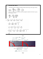
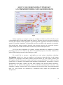
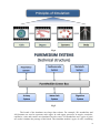
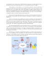
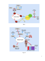
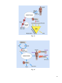
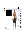
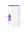
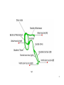
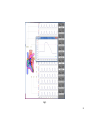
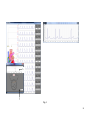
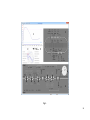
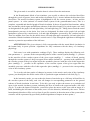
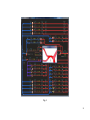
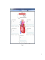
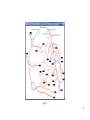
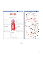
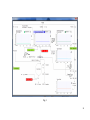
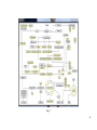
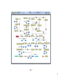
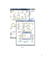
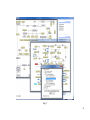
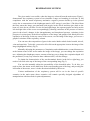
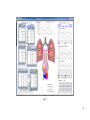
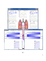
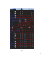
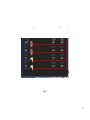
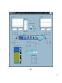
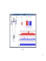
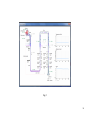
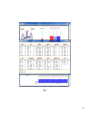
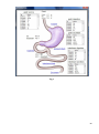
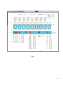
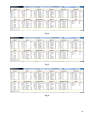
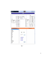
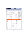
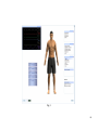
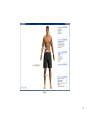
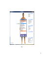
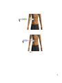
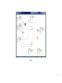
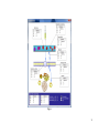
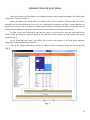
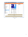
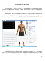
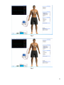
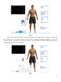
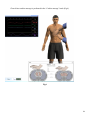
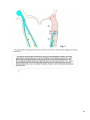
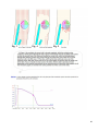
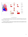
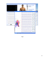
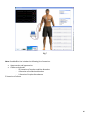
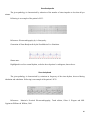
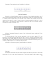
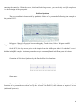
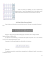
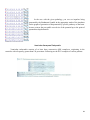
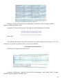
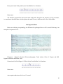
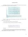
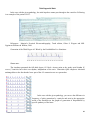
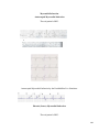
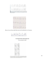
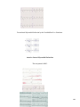
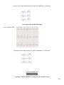
PUREMEDSIM LIVE
PUREMEDSIM LIVE
REAL TIME HUMAN PATIENT SIMULATOR
WITH CARDIO MODULE
USER MANUAL
1
Copyright by PureMedSim Technology Group, Inc. All rights reserved
CONTENTS
ABOUT TECHNOLOGY
BASIC PRINCIPLES
3
3
MAIN MENU OF THE SYSTEM
12
THE MODES
17
GENERAL CHARACTERISTICS OF THE VIRTUAL ORGANISM
17
ORGAN PARAMETERS
18
VIRTUAL HEART
20
CARDIOMYOCYTES
25
HEMODYNAMICS
27
CORONARY SYSTEM
32
GENERAL ORGANISM BIOCHEMISTRY
36
RESPIRATORY SYSTEM
44
GAS EXCHANGE
48
EXCRETORY SYSTEM AND WATER-SALT METABOLISM
52
DIGESTION AND SOAK SYSTEM
57
THE METHODS OF EXTERNAL INFLUENCES
62
FOOD INTAKE
62
DRUGS (EXCRETION/DISTRIBUTION)
65
INTRODUCTION OF SOLUTIONS
72
INSTRUMENTAL METHODS
75
GUIDING PRINCIPLES FOR SETTING UP SCENARIOS
79
RELIABILITY OF THE MODEL’S RESULTS
87
2
ABOUT TECHNOLOGY
BASIC PRINCIPLES
The main task of medical simulation is to obtain a response from a simulator, which is as
close as possible to the real object behavior.
Fulfillment of this task greatly depends on the simulation technology used, and
correspondence of simulation results to the real data is directly proportional to the depth of
simulation (accounting for the highest possible number of factors that influence the final result).
In overwhelming majority of cases, the existing models of medico-biologic processes
take form of a complex set of equations or inequalities of various types with
undetermined coefficients for taking into account diverse factors of influence on the designed
process. In some cases, elements can be presented in defined electric circuits and various
mechanical connections. As an example, let’s view some fragments of respiratory, electrical
activity and hemodynamic patterns, used in medical simulators by well-known developers
(Fig.1, Fig.2, and Fig.3). Various types of equations (differential, regression, nonlinear and
stochastic) serve to describe processes of respiration, hemodynamics, heart activity, muscle work
etc. Modeling results transformed into physical signals can operate widely known mannequin
type systems which are nowadays believed to be the gold standard in medical simulation.
The above-described approach to modeling medico-biological processes appears to be an
extremely interesting one; still, a certain indiscriminate contradiction remains immanent to it.
Mathematical modeling is typically applied when it is unknown how an object under study is
functioning or when it is out of the observers reach. But most processes occurring in an organism
are well-studied and described in detail in terms of biophysics, biochemistry and molecular
biology. Thus, any attempt to present such processes by means of mathematical modeling leads
to substitution of real objects for formal equations.
The imperfections of such models are obvious, including difficulty of perception,
inaccurate reflection of properties and real object behavior, solubility of only strictly defined
tasks, etc. Another common issue is correspondence of a simulator’s performance results with a
real object’s behavior. Any medical simulator, based on such models, even with the best
engineering solutions, has nothing in common with real structure and processes that take place in
the human organism. As a result, time intervals and quantitative indicators of the simulated
parameters are not always accurate.
It is well known that vital activities of the human organism are sustained through various
biochemical processes. And still none of the currently existing systems of medical simulation has
a module of biochemical and enzymatic transformations, and the entire biochemistry of the
organism is accounted by several constants and variables in the equations of the model. This
imposes significant limitations on the use of such systems.
3
EXPIRATORY PHASE
Calculating pressures along the expiratory path from the lung via the upper airway:
Where Ic is the gas flow from the trachea through the cannula to the three-way tap.
Rearranging, we have:
Fig.1
Fig.2
4
Fig.3
Human organism is a complex system, any condition of which can be described by a sum
of interrelated states of individual organs and systems. Therefore, the only accurate approach to
assessing the condition of the organism is a system approach. Application of the above-described
systems of medical simulation of biomedical processes precludes this approach in principle.
Such models may pretty accurately describe some separate processes in a particular organ or
system, but they are unable to link them with an array of other related processes.
All of the above limitations of currently existing approaches to simulation of human
physiology processes cast doubt on the future development prospects of medical simulation in
general. Most leading experts in this field agree on this.
We would like to present a principally new and unique simulation technology
PureMedSim, which is as close as possible to real processes that take place in the human
organism. It is designed in accordance with the principle 'bottom- up': cells, organs, systems, and
the organism (Fig.4). The system’s technical structure is presented in Figure 5. In the core of the
system there is a module of biochemical and enzymatic transformations, presented in a form of
PureMedSim Center Bus. Organs are built from working cells and the stroma (skeleton.).
Working cells are filled with cytoplasm, where biochemical transformations take place with
substances, coming from the blood as food matters enter the blood flow from gastrointestinal
tract, etc. All processes are described by well-known laws, simple for perception and
interpretation.
5
Fig.4
Fig.5
The kernel of the simulator uses large data volume. For example, 541 metabolites and
424 ferments are used to represent each organ. In each organ, processes in arteries, arterioles,
capillaries, veins and venules are simulated. In each vessel, 292 metabolites and 7 types of gases
are used to simulate the passage of the blood. The simulator models 8 types of cells, containing
6
146 metabolites each. In total, nearly 132880 biochemical parameters, excluding physical factors
like pressure in the vessels, heat transmission, etc., are involved to describe 16 organs.
Each subsystem is represented by a set of particular parameters, characterising certain
functions of organs and systems in the human organism. Average values of all parameters in all
subsystems are set by default. Data comes from publicly available medical literature and
websites. All formulas that were used are commonly known and described in textbooks on
Physiology, Biochemistry, Biophysics and Molecular Biology. It is easy to verify conformance
of simulation results to real data, using specially designed tests.
All processes are interrelated in the same way as they are in a real organism. Alteration of
any parameter in any module will result in automatic recalculation of values of all parameters,
related to it.
Thus, we do not apply purely mathematical methods in modeling, since the language of
mathematics proves to be most applicable when describing physico-technical objects and is of
little use for many fields of medical science and biology. This is why our description of objects
is based upon how they function in reality. The process is laborious indeed, but it yields the
perfect result – the complete correspondence between a model and reality.
The virtual organism consists of cells just like the real one; it can generate its own ECG;
it contains all vital biochemical processes just like the real organism; in the Hemodynamic
Mode, the blood distributes nutrients to all organs; respiratory mechanics correspond to real
processes in the diaphragm of the lungs, etc. Furthermore, all of the above-mentioned processes
are taking place in real time.
Methodology for computing, computational algorithms, presentation and organization of
data sets, sets changing in time (instruments of virtual movement) are absolute know-how.
Conformity of the simulated results is verified by specially selected test tasks. Main relations of
the system are shown in the schemes below (Fig.6-Fig.12).
Fig. 6
7
Fig.7
Fig. 8
8
Fig. 9
Fig. 10
9
Fig. 11
Fig. 12
10
The following may be regarded as the fields of use for products developed through the
technology described herein.
1. Education
Our technology is able to cover virtually all fields of medicine. Unlike all other medical
simulation systems, it provides an opportunity to study normal physiological processes and
pathogenesis mechanisms of diseases on any representation level: an organism as a whole, a
separate organ, a cell. Such technologies are of good use for students studying theoretical and
clinical disciplines, like biophysics, normal physiology, biochemistry, cardiology, nephrology,
endocrinology etc. Physicians of any qualification level can significantly improve their
knowledge and practical skills working on various technological levels of a virtual organism
representation. In principle, medical simulators developed on such technologies’ basis, may
change in future the medical education system at large. From the development perspective, it
will be achieved by adding any number of scenarios of various pathological conditions and
corresponding treatment options. The kernel of the system will remain unchanged. In
perspective, this approach could totally change the entire system of medical education.
2. Research
Modern simulators are not currently in use in this area. Our approach opens up some
interesting prospects. For example, you can change any parameter you want to research (enzyme,
vascular permeability, etc.) and explore the changes, including long term, taking place in the
organism as a whole or in any of its organs. The data obtained as a result of the simulation can be
compared with real practical data. This approach may significantly increase the efficiency of
biomedical research.
3. Clinical Practice
This is the most promising future direction for the use of medical simulators. Existing systems
won’t do here in principle. Systems, developed on the basis of our technology, will allow one to
simulate the tactics and predict the results of any treatment, which undoubtedly will increase the
effectiveness of diagnostic and treatment process.
11
MAIN MENU OF THE SYSTEM
Once the system is started, the main menu appears (Fig.1)
In the center of the main menu, there is a screen simulator (1). Apart from tactile
sensations, it displays all the main externally observable processes: breathing, heartbeat,
blinking, sweating, skin discoloration, loss of body weight. In our technology (refer to the
section "About technology"), the on-screen simulator (virtual organism) is the equivalent of a
living organism and is built like one, that is, it consists of cells that form organs, which are
controlled by systems, etc. Thus, in our system, the concept of the on-screen simulator and the
concept of the organism are identical. Our on-screen simulator generates physiological processes
of the organism, indicators of which are displayed in real time on the monitor, on the left hand
side of the main menu (2). The monitor takes form of a separate window, which can be moved
around the screen. To enlarge the image, you need to double-click at the top of the monitor
window (Fig.2).
The right hand side of the main menu contains the following:
3 – Menu of scenarios of various pathological processes;
4 – Menu of certain instrumental interventions;
5 – Menu of external influences: food, drugs, solutions, etc.
6 - Line selection of the study object (organism as a whole, individual organs and
systems);
7 – Menu of different modes, which reflect functions of different organs and systems in
the organism;
8 – Clock, recording running time of the simulator and "Start\Stop" button, which allows
suspending and restarting the work of the simulator.
The system operates on several levels. At the first (general) level, you are able to select
any scenario that interests you from the appropriate menu and observe real-time changes of
parameters on the monitor and the external state of the simulator. After that, you can select the
appropriate methods of instrumental and/or external influences from the various menus to bring
the monitor parameters to a complete normalization. This first level to a certain extent matches
the ideology of all currently used simulation systems, including the mannequin type.
At the general level, only two modes are available on the menu: "Patient characteristics"
and "Systemic metabolism". In the "Patient characteristics" mode, you can find all physical
characteristics (weight, height, age) and quantitative values of the basic substances in the virtual
organism. In the "Systemic metabolism" mode, real-time quantitative indicators of basic
metabolic processes in the organism are displayed. If the nutrition is not set, for example, when
you first start the simulator (the indicators of fats, proteins and carbohydrates in this mode will
be equal to 0), and biochemical processes will occur, as in the real organism at the expense of
proteins, located in the muscle tissue, carbohydrates, formed as a result of glycogen in the liver
12
and fat from the subcutaneous tissue. Full description of these modes can be found in the
corresponding sections.
At the next level, you can monitor real-time processes in specific organs and systems of
the simulator, as in the normal physiological state, as in any selected scenario with any
instrumental and/or external influences on the simulator. To access this level, you need to place
the mouse on the image of the simulator (anywhere). At this, organs and systems of the organism
will be outlined (Fig.3). To select an organ that interests you, it is necessary to place the mouse
precisely on the image of the desired organ (when you do this, the image becomes brighter) and
make a left click. As a result, all modes related to the selected organ will appear on the menu.
For example, when the heart is selected (Fig.4), the following modes appear: "Organ
parameters", "Hemodynamics", "Heart", "Coronary system", "Organ metabolism" (refer to the
description of these modes in corresponding sections.)
The third level is the cell level. At this level, you can study individual processes in the
cells of certain organs. It is possible to access this level in certain modes, such as the "Heart"
mode (see description.)
All three levels can also be selected simultaneously. For example, you can set a scenario
for pathological cardiac activity and observe changes in parameters on the monitor, then select a
method of treatment and the organ, e.g. the heart, and observe all the occurring processes
(including at the cellular level) in the corresponding modes.
Clock (8) displays the time of virtual life of the on-screen simulator after the system is
started. When you exit the system, the time is automatically reset.
The work of the simulator can be paused and restarted with the click of the "Start \ Stop"
button. This button is also used when it is necessary to view the value of any indicator at any
given time. You can also use this button if you want to observe the work of the simulator in
several windows of different modes simultaneously. To do this, you will first have to stop the
simulator with the help of this button, then set all necessary windows and restart the simulator.
13
1
2
3
4
5
6
7
8
Fig.1
14
Fig.2
15
Fig. 3
Fig. 4
16
THE MODES
GENERAL CHARACTERISTICS OF THE VIRTUAL ORGANISM
The given mode is only accessible, when the organism as a whole is selected from the
main menu. The “Patient Characteristics” mode contains physical characteristics (weight, height,
age) and quantitative values of the basic substances in the virtual organism, which form the basis
for our screen simulator model (Fig.1).
Fig.1
17
ORGAN PARAMETERS
This mode is only accessible, when a particular organ is selected from the main menu.
Once “Organ Parameters” are selected from the main menu, a hierarchical database
structure will appear, containing all the parameters of the selected organ that are being used by
the simulator in its work. Fig.1 demonstrates such a structure (search tree) on the example of a
lung. Then, you can search for the relevant information by scrolling down the tree and leftclicking on the corresponding rectangular icons, marked with a + sign in the center. Fig. 2 shows
a sequential search for information on the quantitative composition of various vitamins in the
extracellular fluid of the lungs.
If you conduct the search, while the simulator is running (without resorting to the
Start\Stop buttons), it means that the information can get updated in the course of the search. To
get updated real-time information, you need to make a double left-click on the name of this mode
is the mode menu.
Fig. 1
18
Fig. 2
19
VIRTUAL HEART
The given mode is accessible, when the heart is selected from the main menu.
The unique electrophysiological model of the heart provides an opportunity to observe
and study the heart rate pattern in real time, including all necessary cellular mechanisms:
generation of bio-potential actions of individual cells in different sections of the heart in the
course of the excitation wave expansion and mechanisms of emergence of rhythm disturbances.
The overall picture, displayed when this model is selected, is shown in Fig.1.
1 – Virtual image of the heart is displayed on the screen of the simulator. The heart is
beating in real time with a fixed rate in full accordance with the actual physiological heartbeat
pattern in various sections of the heart. The heart rate is set in the main menu of the system.
Conduction path is highlighted in green. It is shown separately in Fig.2, where the names
of corresponding areas are provided. Areas, responsible for the contraction in corresponding
sections of the heart, are additionally marked with red dots in Fig.2.
2 – Real time graphs of generation of bio-potential actions of individual cells in different
sections of the heart.
3 –Names of the corresponding areas of the conduction path and the main characteristics
of the heartbeat at any given area. To zoom in on any particular section of any particular graph,
all you need to do is left-click on the line with the name of the section (Fig.3).
4 –Yellow squares mark some points on each section of the conduction path. When you
enable them in the interactive mode, you can explore the mechanisms of emergence of single
extrasystoles in different sections of the heart. More complex rhythm disturbances will be set in
the form of specific scenarios in the main menu of the system (these scenarios will be set in the
form of specially designed algorithms, allowing you to manipulate these points.)
To study the mechanism of emergence of rhythm disturbances in an interactive mode,
you need to left click the corresponding yellow square (each of them representing a certain area
of the conduction path.) As a result, an interactive window 5 is displayed (Fig.4). Here you need
to place the mouse anywhere on the line of specified time interval, set the excitation pulse to 6
and press Power. In this case, a certain section of the heart, associated with the corresponding
yellow square, is artificially stimulated. This stimulation leads to the emergence of the
corresponding extrasystole that can be seen on the ECG. In addition, the corresponding heartbeat
abnormality will be displayed in real-time on the virtual heart image.
In real life, the same impulses can arise in these sections of the heart due to a variety of
reasons that can be known, unknown or accidental at times.
In some cases, the set excitation pulse may not cause any changes in the model (it all
depends on the period in what the excitation pulse is set). As with the real working heart, it
means that we are in period of refractoriness, when a certain section of the heart cannot be
excited for some time.
20
3
1
4
2
Fig.1
21
Fig.2
22
Fig.3
23
6
5
Fig. 4
24
CARDIOMYOCYTES
In this mode, we study cellular mechanisms of action potential generation in different
sections of the conduction path. The given mode is accessible, when the heart is selected from
the main menu.
Main menu of this mode is shown in Fig. 1.
1 - Generation of real-time graph of action potential of the cell from a selected area of the
conduction path.
2 - Scope of selection of corresponding sections of the conduction path; to make the
selection, you need to place the mouse on the name of the desired section and left-click it.
3 - Real time state of the corresponding cell in the course of generation of bio-potential
actions. All quantitative indicators of the ion content in the cell and work of sodium- potassium
and calcium pumps, as well as the time intervals are in full correspondence to actual indicators in
a living cell. This is proved by the complete match of the generated pulse parameters with the
literature data.
4 - Real time state of ion channels in the corresponding cell. All shown quantitative
electrical parameters and time intervals correspond to actual processes in a living cell.
5 - Switch that enables you to study cellular mechanisms in slow motion.
25
3
1
2
5
4
Fig. 1.
26
HEMODYNAMICS
The given mode is accessible, when the heart is selected from the main menu.
In the Hemodynamic Mode of our simulator, you are able to observe the real-time blood flow
through the vessels in greater, lesser and cardiac circulation (Fig.1). Arrows indicate the direction of the
blood flow. The arterial circulatory system is highlighted in red, the venous system – in blue, and the
portal system - in violet (mixture of arterial-venous system in the gastrointestinal tract). This is a
complete, expanded and detailed graph of blood circulation. It shows all possible blood motions, taking
into account the paired organs and different schemes of their blood supply. For paired organs, two icons
are designated on the graph: left and right kidney, left and right lung, etc. Taking into account the actual
hemodynamic processes in the brain, four icons are designated for them on the graph: left and right
hemisphere (powered by carotid artery), left and right hemisphere (powered by the vertebral artery.)
There are another four icons for the muscle tissue: left and right upper extremities, left and right lower
extremities. Blood circulation of the heart is carried out in 3 ways: through the right heart or through the
anterior or posterior myocardium of the left heart.
ATTENTION!!! The given scheme is fully correspondent with the actual blood circulation in
the human body in prone position. Algorithms are fully consistent with the theory of circulatory
physiology.
Each route is set with quantitative readings (Fig.2). These readings display the following realtime parameters: 1 – pressure in the corresponding arteries of the vascular system (mmHg); 2 – pressure
in the arterioles of the vascular system of the given organ (mmHg); 3 – volume of blood, passing
through the vascular system of the given organ in one minute (ml/min); 4 – pressure in the capillaries of
the vascular system of the given organ before the metabolic processes with the cells of this organ take
place (mmHg); 5 - pressure in the capillaries of the vascular system of the given organ after the
metabolic processes with the cells of this organ take place (mmHg); 6 – pressure in the corresponding
veins of the circulatory system.
To view the real-time graphs of changes in pressure in the arteries and veins of the circulatory
system, you should place the mouse on the icon of a particular organ and make a left-click (Fig.3).
In the interactive mode, you can reduce the lumen of arterioles up to a full stop in blood flow in
the vascular system of the body, and view all changes in corresponding parameters on the general
scheme of blood circulation in real time. To do this, you need to place the mouse on a particular red
arrow in the arterial circulatory system, indicating the flow of blood to the organ and make a left click
(Fig.4). To reduce the lumen of arterioles, you need to place the mouse on the icon with an image of a
hand, and holding the left button of the mouse, move it in the direction, indicated by the arrow. Various
hemodynamic disorders will be set in a form of specific scenarios in the main menu of the system (these
scenarios will be represented by specifically defined algorithms of impact on these points.)
27
Fig. 1
28
6
5
4
3
2
1
Fig. 2
29
Fig.3
30
Fig. 4
31
CORONARY SYSTEM
The given mode is accessible, when the heart is selected from the main menu.
Main menu of this mode is shown in Figure 1. In the center of the heart icon, you can see
three coronary arteries: the right one (1), left anterior (2) and left posterior (3) ones. On the
graphs, surrounding the heart icon, you can observe the oxygen flowing through the coronary
vessels of the corresponding sections of the heart: right heart (4), posterior part of the heart (5),
the apex (6), anterior part of the heart (7) and left heart (8); 9 - lumen control for individual
sections of the coronary system.
When you press the MAP button, a graph of coronary arteries will appear, indicating the
blood pressure in each branch (top figure - the pressure at systole, bottom figure - the pressure at
diastole) and the corresponding flow rate of the blood (Fig.2).
In this mode, it is possible to simulate pathological vascular permeability in any part of
the coronary system (Fig.3). To do this, you need to highlight any branch of the coronary system
by left-clicking it (when you do so, it will be highlighted in green.) The selected part of the
coronary system will be also highlighted in green on the graph. After this, you need to reduce the
lumen of the given area, using the regulator (9). As a result, all corresponding graphs of oxygen
in the main menu, as well as pressure and flow rate indicators on the graph will change.
When the entire system is ready, it will, in its turn, lead to corresponding changes in the
ECG of the heart and in the main menu on the monitor, as well as in all other relevant systems
of the organism.
32
9
3
4
8
1
2
7
5
6
Fig. 1
33
Fig. 2
34
Fig. 3
35
GENERAL ORGANISM BIOCHEMISTRY, METABOLIC PROCESSES IN
INDIVIDUAL ORGANS
The Biochemistry Module is the core of the entire simulation technology PureMedSim,
used to design the simulator at hand.
This Module allows you to observe all the known biochemical changes in the human
body in real time. As a result, you get a visual representation of complex polyhedral relations
between the various biochemical processes in the organism.
The Biochemistry Module is represented in the main menu of the simulator by two
modes: systemic metabolism (overall metabolism) and organ metabolism (metabolism in specific
organs). Systemic metabolism mode is only accessible, when the organism as a whole is selected
from the main menu. Organ metabolism mode is only accessible, when a certain organ is
selected from the main menu.
Once systemic metabolism is selected, the main menu of the mode appears (Fig.1). Here
are presented the main characteristics of the overall metabolism in the form of graphs and
quantitative values. The graphs demonstrate the following:
1 – Glucose intake by cells of various organs (from the blood). The brain is set here by
default, but you can also select any other organ by left-clicking an arrow on the line above the
graph, allocated in the light green rectangle.
2 – The overall level of glucose in the venous blood in various organs. The brain is set
here by default, but you can also select any other organ by left-clicking an arrow on the line
above the graph, allocated in the blue rectangle.
3 – Insulin and glucagon concentrations in the venous blood in various organs. The brain
is set here by default, but you can also select any other organ by left-clicking an arrow on the line
above the graph, allocated in the dark green rectangle.
4 – Glucose synthesis from liver and kidney proteins.
5 – Urea concentration in the blood.
All other key indicators of general organism metabolism are presented by quantitative
values. Arrows on the graph show the direction of the corresponding biochemical processes.
The input data for this mode are quantitative indicators of consumed food (set in the
“Food” mode), physical characteristics of the human (set by default), certain environmental
conditions associated with gases (set by default). Accordingly, any changes in these indicators
will lead to corresponding changes of the simulated biochemical processes. If the nutrition is not
set, for example, when you first start the simulator (the indicators of fats, proteins and
36
carbohydrates in this mode will be equal to 0), and biochemical processes will occur, as in the
real organism, at the expense of proteins, located in the muscle tissue, carbohydrates, formed
from glycogen in the liver and fats from the subcutaneous tissue.
Once organ metabolism is selected (the main menu shown in Fig.2), all chains of
biochemical transformations of different ingredients in a specific organ will be presented (the
organ is selected on the on-screen simulator), as well as all subsequent biochemical
transformations of derived substrates, including the Krebs cycle and the ornithine cycle, the
energy accumulation processes in the cells of the organism and the output of the final irreversible
breakdown products.
Here and further, for your convenience we will be using different colors in the names of
the corresponding substances. Highlighted in yellow are the key substances, presented in the full
cycle of transformations. For example, by left-clicking the yellow rectangle, labeled glucose, you
will get a complete graph of biochemical transformations of this substance in the organism
(Fig.3).
To obtain a real-time quantitative value of any key substance in a given scheme of
transformations, you need to left-click the yellow rectangle with the name of a particular
substance. As a result, the chemical formula of the substance and its quantitative value at a given
time will be presented (for example, the quantity of fructose-6-phosphate in Fig.4).
Red color marks the beginning or the end of a chain of transformations on this scheme
(entry point from the main menu of the regime). Blue color highlights the substances that are
attached or detached from the key substances directly in the course of a corresponding reaction
(quantitative values are not displayed). Pink color highlights intermediate substances, formed in
the process of metabolism, which have not yet completed their biochemical transformations in
this scheme and can be used in other schemes (quantitative values are not displayed). Green
color highlights the substances, consumed in the process of metabolism (quantitative values are
not displayed). Dark blue color highlights the names of specific parts of the scheme of
transformations.
In the main menu of this mode (Fig.2) some substances are highlighted in gray. The
quantitative values of some of them can be seen in the mode of systemic metabolism, while some
of their schemes are not detailed (quantitative values are not displayed).
All metabolites transformations from one to another are regulated by relevant enzyme
systems, indicated on all graphs in the form of round icons, labeled with E. An average enzyme
activity is set by default. At the left-click on the icon, labeled as enzyme system, a window
appears with the corresponding indicator of activity of the given enzyme. For example, Figure 5
demonstrates the activity of the glucose-6-phosphateisomerase enzyme (on the graph of glucose
transformations, found in Figure 3, this enzyme is located between glucose-6-phosphate and
fructose-6-phosphate).
37
The user can manually change quantitative indicators of activity of any enzyme and thus
alter the course of any chosen biochemical process. Various metabolic disorders will be set in the
form of specific scenarios in the main menu of the system (these scenarios will be specially
designed algorithms of impact on the activity of the corresponding enzymes).
38
2
1
3
4
5
Fig. 1
39
Fig. 2
40
Fig. 3
41
Fig. 4
42
Fig. 5
43
RESPIRATORY SYSTEM
The given mode is accessible, when the lungs are selected from the main menu. Figure 1
demonstrates the respiratory system of our simulator. Lungs are breathing in real time, in full
compliance with the actual respiratory mechanics: negative pressure builds up in the pleural
cavity due to contractions of the diaphragm muscle (ATP energy is used here.) The blood from
the heart enters the lungs, gets saturated with oxygen in the alveoli and then goes back to the
heart, all this also in real time. For the left and right lungs, the separate graphs are built (on the
left and right sides of the screen correspondingly), showing variations in the pressure of various
gases in the alveoli, changes in the intrapulmonary and intrapleural pressure, variations in the
pressure of various gases in the blood capillaries of the lungs, and graphs of the blood pH in the
capillaries of the lungs. In the top center of the screen, over the image of the lungs, you can see a
graph of variations in the respiratory volume.
You can trace the composition of gases in the entire inhale-exhale chain: bronchi, alveoli,
veins and arterioles. To do this, you need to left-click on the appropriate icon on the image of the
lungs (highlighted in blue) (Fig.2).
Manually adjusting the parameters of inspiration and exhalation time (control buttons are
at the bottom center of the screen under the image of the lungs), you can change the respiration
rate. Adjusting the diaphragm creates vacuum, allowing you to change the respiration depth. All
the parameters, in any way related to these characteristics, will also change.
To obtain the characteristics of the aero-haematinic barrier in the left or right lung, you
need to left-click at the top of the image of the corresponding lung (Fig. 3).
You can also manually adjust the permeability of the bronchial tubes. To do this, you
need to place the mouse on the hand icon in the corresponding part of the lung, and pressing the
left button of the mouse, move it in the direction indicated by the arrow.
Various malfunctions of the respiratory system will be set in the form of specific
scenarios in the main menu (these scenarios will contain specially designed algorithms of
manipulations with described set point adjustments.)
44
Fig. 1
45
Fig. 2
46
Fig. 3
47
GAS EXCHANGE
In the "Gas Distribution" mode, you can observe the gas exchange in various organs in real
time. When you start this mode, a window with a graph of the patient’s gas exchange will appear on
the screen (Fig.1). It is a complete, fully-fledged and detailed graph of gas exchange against the
hemodynamic background.
PLEASE NOTE!!! This graph is fully consistent with the real gas exchange in the human
organism.
Each path has set numerical values (Fig.2). These figures correspond to the following realtime parameters: 1 - hemoglobin oxygen saturation in the corresponding arteries of the vascular
system, 2 - hemoglobin oxygen saturation in the corresponding arterioles of the organ’s vascular
system, 3 - hemoglobin oxygen saturation in the corresponding veins of the vascular system.
In order to view a complete real-time gas exchange in a particular organ, you need to place
the mouse on the icon with the image of a specific organ on the graph and make a left click (Fig.3).
On the right hand side of the graph in Figure 3, you can see the characteristics of various
gases prior to the gas exchange processes in the given organ and on the left hand side - after the gas
exchange processes.
Various gas exchange disorders will be set in the form of specific scenarios in the main
menu of the system.
48
Fig. 1
49
2
3
1
Fig. 2
50
Fig.3
51
EXCRETORY SYSTEM AND WATER-SALT METABOLISM
The given mode is accessible, when the kidneys are selected from the main menu. Main
menu of this mode is shown in Figure 1. On the left, you can find an icon for the excretory
system: kidneys, bladder and blood vessels that feed the kidneys. Generation of urine in the
bladder happens in real time. In order to view full information on the biochemical composition
of urine, you need to left-click on the line, called Urine, highlighted in blue and located under
the bladder icon.
Options Nephron right and Nephron left allow you to observe in real time the uropoiesis
mechanism in the left and right kidney accordingly. When you left-click any of these icons, an
interactive image, shown in Figure 2, will appear. It demonstrates nephron, a functional element
of uropoiesis, consisting of the glomerulus, a tangle of vessels, where the primary urine is
filtered, the descending limb of Henle, the loop of Henle and the collecting duct.
Directly next to the glomerulus icon, you can find indicators, displaying readings of
incoming and outgoing hydrostatic blood pressure, as well as the pressure of urine in the
descending limb of the nephron. Along the entire loop, you can see indicators of osmolar
reabsorption, the osmotic gradients that lead to the second phase of uropoiesis.
On the right, you can find three graphs. The top and the middle graphs display the
dynamics of hormone levels in the blood, regulating the second phase of uropoiesis. The bottom
graph displays diuresis.
Let us go back to the main menu of this mode (Fig.1.) In the top center of the screen,
there is a test tube icon, containing the total amount of blood in the organism. Specific numerical
values of blood in ml and haematocrit levels can be found above and to the left of the test tube
icon respectively.
At the top right corner of the main menu, there are three rectangular columns with
dynamically changing content, determining (from left to right) the total water content in the
blood of the organism, water content in the extracellular environment of the entire organism and
water content in the intracellular environment of the entire organism. Specific numerical values
of water in ml. are indicated under each column. Inside the columns (at the top), the
corresponding values of the osmotic concentration of substances in water are displayed.
In order to obtain full information on the biochemical composition of substances in the
blood, the composition of substances in the extracellular environment and the composition of
substances in the intracellular environment of the organism, you need to left-click on the Blood,
Extracell, Intracell lines respectively, highlighted in blue and located under the rectangular
columns. Figure 3 shows the result of such action on the example of the biochemical
composition of the blood. To do the same but in terms of concentration, it is necessary to leftclick on the appropriate mmol/l lines, also highlighted in blue but located a bit lower. Total
biochemical composition of all substances in the organism (blood + extracellular environment +
intracellular environment) is determined by left-clicking the Sum line, highlighted in blue.
Finally, the biochemical composition of the blood cells is determined by left-clicking the blue
Cells line.
At the bottom right corner of the main menu, there are rectangular columns of a smaller
size with dynamically changing content, determining the water content in the blood of individual
52
organs (top), the extracellular water content of individual organs (middle) and the intracellular
water content of individual organs (bottom.) Similarly, specific numerical values of water in ml.
are displayed under the respective columns, while the osmotic concentration of substances in the
water is provided inside the columns (at the top).
53
Fig. 1
54
Fig. 2
55
Fig. 3
56
DIGESTION AND SOAK SYSTEM
This mode is only accessible, when the gaster is selected from the main menu.
"Digestion and Soak" mode present interest only, when the food has entered the organism.
Without any food, you will only see the secretion of gastrointestinal juices that are being absorbed
into the blood. Therefore, before using this mode, you need to go to the menu of external
influences, select the "Food" mode and set the patient’s diet.
In the "Digestion and Soak" mode, you can observe in real time secretion of gastrointestinal
juices, enzymatic degradation of food products and their absorption into the blood.
The menu of the given mode is shown in Figure 1. The following real-time indicators are
shown in the corresponding tables:
- Gastr source – gastric substances, received with food;
- Gastr digestion – final product of the gastrointestinal digestion;
- Gastr secretion – secretion of gastric juices and enzymes in the stomach;
- Intestinum digestion – final products of the gastrointestinal digestion;
- Intestinum secretion – secretion of digestive juices and enzymes in the intestine.
If you left-click on the lines, highlighted in blue, you will get real-time information on the
following processes:
- Enzyme – protein breakdown in the stomach (Fig. 2);
- Digestion – breakdown and absorption of food ingredients in the intestine (Fig. 3). The
speed of red dots on the image corresponds to the speed of absorption of the given metabolite;
- Stomach (fluid) – substances currently in the gastric cavity (Fig. 4);
- Intestinum (fluid) – substances currently in the intestine (Fig. 5);
- Excrement – substances currently in the feces (Fig. 6).
By introducing changes to enzyme activities, we can simulate any pathology of nutrition in
the intestine and the stomach.
57
Fig. 1
58
Fig. 2
59
Fig. 3
60
Fig. 4
Fig. 5
Fig. 6
61
THE METHODS OF EXTERNAL INFLUENCES
FOOD INTAKE
Main Menu of this mode is shown in Figure 1. At the bottom right corner, there is a window
with a list of various food products. To set a specific diet, you need to select food products from the
list one by one, indicating the quantity of each product in grams. You need to press Ok after each
selection, and then the selected product will be displayed in a window at the bottom left corner of
the menu (the window of selection results).
Following each selection of relevant food products, quantitative composition of all their
ingredients (proteins, fats, carbohydrates, vitamins, etc.) will be automatically displayed at the top
part of the mode menu.
For user convenience, certain diets were set in the system in advance. To choose them, you
need to left-click on the lines of breakfast, dinner and snack, highlighted in blue, and found in the
lower central part of the mode menu. At that, the window of selection results will display the entire
list of products of the given diet, and at the top - quantitative composition of ingredients of all
products on this diet (Fig. 2).
In order for any given diet to enter into the system, you just need to close the main menu of
the mode. You will find confirmation for this in the "Digestion and Soak" mode.
We would like to remind you that our simulator works like a real organism, therefore the
diet is very important when you want to study any processes, related to biochemical
transformations.
62
Fig. 1
63
Fig. 2
64
DRUGS
Diagram of Drugs Excretion from the Organism
Diagram of Drugs Distribution in the Organism
In the Drugs Mode of the system, you can select various drugs from the database and
introduce them into the virtual organism. When you select this mode, you’ll see the window,
shown in Figure 1. On the left-hand side of the window, you can find a box with the names of
various groups of drugs. In order to select a certain drug from any group, you need to left-click
its name. If these actions are performed correctly, the image of a syringe, filled with liquid, will
appear on the screen (Fig.2). The mode accounts for all possible ways of drug introduction: per
oral, intravenous, endermatic and intramuscular. To introduce a drug, you need to place the
mouse on the syringe icon, left-click it and drag the syringe into the designated zone, marked
with a dotted triangle. This will open a window with a database of corresponding drugs (Fig.3).
Following that, you need to select the desired drug, set or alter its dosage (for many drugs dosage
is already set by default) and click Ok. If the drug is administered orally in a form of a pill, do
not forget to add 30-50 ml of liquid to wash it down. Then, place the mouse at the top of the
syringe plunger image, left-click it and holding the button, progressively move the plunger to the
end (Fig.4). When the drug introduction is complete, the system automatically returns to the
main menu.
Drugs Excretion Mode allows to get a real-time excretion diagram of all drugs,
introduced in the process of simulation (Fig.5).
Drugs Distribution Mode allows to get a real-time distribution diagram of all drugs,
introduced in the process of simulation (Fig.6).
65
Fig. 1
66
Fig. 2
67
Fig. 3
68
Fig. 4
Fig. 4
69
Fig. 5
70
Fig. 6
71
INTRODUCTION OF SOLUTIONS
In the given mode, various solutions are introduced into the virtual organism through a drip. Main Menu
of this mode is shown in Figure 1.
On the left side of the menu, there is a window with a list of solutions. Solutions that you wish to
introduce can be selected from the list one by one, indicating the quantity in ml and a certain infusion rate
(default rate is 60 ml \ min). You need to confirm each selection by pressing the Ok button. At that, the selected
solution will be displayed on the right side of the menu in the window of selection results (Fig.2).
In order for any given solution to enter into the system, you just need to close the main menu of the
mode. At that, the image of a drip will appear in the main menu of the system next to the image of the screen
simulator (Fig.3).
In the "Water and ions" mode, you will be able to observe the balance of all fluids in the organism,
taking into account the introduced solutions.
Also, in the "Drugs" mode there will now be added an option to introduce drugs directly into the drip
(Fig.4).
Fig. 1
72
Fig. 2
73
Fig. 3
Fig. 4
74
INSTRUMENTAL METHODS
Equipment, required at any given moment, can be selected from the menu of instrumental methods,
located on the right side of the Main Menu. When the electrocardiogram is selected, a window appears,
generating 12-lead ECG in real-time (Fig.1). If you wish to enlarge any of the leads, you need to left-click the
corresponding image.
ATTENTION!!! This electrocardiogram is generated by the given virtual heart, and its points are
calculated every instant as a geometric sum of bio-potential actions of all cells in all corresponding sections
(this is an extremely difficult mathematical task; methods of calculation and computational algorithms are not
listed here as they are an absolute know-how.) THIS IS EXACTLY WHAT HAPPENS IN REAL HEART!
Fig.1
Defibrillation is used in the following modes: "Defibrillation monophasic" (Fig.2), "Defibrillation
biphasic" (Fig.3) and "Cardioversion biphasic" (Fig.4). The difference between these modes lies in the power
discharge and the pulse shape. Both, the power discharge and the pulse shape, can be found on the exterior body
panel. To start the procedure, you need to left-click the Power button.
75
Fig.2
Fig.3
76
Fig.4
In the "Pacing rate" mode (Fig.5) an external pacemaker can be connected. You will need to specify the
area of stimulation, i.e. the place where the electrode should be installed through the esophagus, as well as the
required pulse rate (a frequency of 79 pulses per minute is set in the system by default). Red star marks the area
of stimulation, set in the system by default.
Fig.5
77
Closed-chest cardiac massage is performed in the “Cardiac massage” mode (Fig.6).
Fig.6
78
GUIDING PRINCIPLES FOR SETTING UP SCENARIOS OF VARIOUS
PATHOLOGICAL CONDITIONS
Work with scenarios involves several levels. At the first (general training) level, following the selection
of a certain pathological condition from the system’s menu of scenarios, the work of the simulator gets
suspended, and a window with a detailed description of the pathogenesis mechanism appears. In this window,
pathogenesis mechanisms are also presented in the form of special graphs that demonstrate in real time the
origins and development of pathological processes, characteristic of the given condition. At the second (specific
training) level, you can introduce changes in the course of pathological processes with the help of special
interactive controls, also found in the window, containing the scenario description. At the third (control) level,
following the selection of a certain pathological condition, the scenario window closes immediately, but the
simulator continues working with the new parameters, automatically tuned to the given pathology. State of the
monitor and the screen simulator will also change according to the given condition. The name of the selected
pathology will appear in the line of selection of study objects in the main menu. At this level, you need to
administer treatment, consisting of drugs and \ or instrumental methods. To complete your work with the
simulator, you need to reset all parameters back to normal. You can return to the scenario window at any time
by left-clicking the name of the scenario in the line of selection of study objects in the main menu.
By way of example, let us review a scenario of ventricular paroxysmal tachycardia. After selecting the
given pathology from the list of scenarios, a window with a detailed description of the pathogenesis mechanism
appears. Next, we are offering to your view a complete scenario window:
79
Ventricular Paroxysmal Tachycardia
Fig. 1
80
Fig. 2
81
Fig. 3
Fig. 4
Fig. 5
82
83
The end of the scenario
At this, the general training level of the scenario completes. At the special training level of the scenario,
the user can change characteristics of the pulse in all four zones of the nidus, thus controlling the pathogenesis
mechanism of the given pathology.
Finally, at the control level, when you close the window of the given scenario, the simulator will start
working with the new parameters, as shown in Figure 6. Appropriate treatment, such as defibrillation, will result
in recovery of all initially set parameters (Fig. 7).
84
Fig.6
85
Fig.7
Note: PureMedSim Live includes the following list of scenarios:


Hypertension and hypotension
Cardiac arrhythmias
- 11 Scenarios of impulse condition disorders
- 4 Scenarios of conduction disorders
- 1 Scenario of rhythm disturbances
5 Scenarios of Infarcts
86
RELIABILITY OF THE MODEL’S RESULTS
All systems of medical simulation, based on traditional models, have an issue with the reliability of their
results. This can be explained by the fact that any object of study (organ, tissue, system) is taken by these
systems as a whole, with no regard of its internal structure. Such approach involves high level of abstraction,
meaning that the internal processes inside the object are not taken into account. The task of medical simulation
is to obtain such data from the simulator, which is as close as possible to that of the real object with the same
input characteristics. That said, the data cannot be large a priori.
Systems, based on our technology, involve low level of abstraction, because they are built from a single
cell to the whole organism. Therefore, the question of their reliability is considered very differently. Our system
uses about 130,000 parameters to describe the internal structure of all objects of study. Each parameter is within
the range of statistical norms and can be found in patient characteristics and organ parameters, where it can be
easily compared with the data of any literary source. Parameters, generated by the system itself as a result of
certain dynamic functions, can also be easily verified at any stage, because the algorithms of dynamic functions
correspond to real processes in the organism and are based on well-known biochemical and biophysical laws.
The main reliability criterion of the model is assessment of the signals, generated by the simulator:
action potentials in all parts of the conduction path of the heart, ECG, hemodynamic and respiratory
characteristics, enzymatic activity, etc. All of these signals are displayed in real time on the screen of the
simulator and can be compared with corresponding signals of the real organism with similar physical
characteristics. The comparison will show full consistency with the real organism. Inversely, as these signals are
generated at the internal structure level of any object of the model, their consistency with real signals
determines reliability of all internal functions and parameters.
Unlike all other systems of medical simulation, our technology makes it possible to study the
pathogenesis mechanisms of various pathological conditions at any level of representation: the organism as a
whole, individual organs and cells (refer to the previous section of documentation). Once again, the reliability
criterion of any scenario is in assessment of the signals, generated by the system, and their comparison to the
corresponding signals of real patients with similar proven diagnoses.
By way of example, we will demonstrate comparison results for all types of arrhythmias that can be
simulated by the system.
AV Bigeminy
AV bigeminy is a rhythm disturbance, where each reduction of sinus is followed by an extra systole.
Following is an example of the patient’s ECG (arrows point at the extra systoles of the AV node):
References: Marriott’s Practical Electrocardiography, Tenth edition, Galen S. Wagner and MD.
Lippincott Williams & Wilkins, 2001.
87
Generation of AV Bigeminy by the PureMedsim Live Simulator:
AV Nodal Tachycardia
Reciprocating tachycardia is supported by the mechanism of the atrioventricular nodal micro-reentry.
Following is an example of the patient’s ECG (arrows point at the retrograde P waves):
References: Marriott’s Practical Electrocardiography, Tenth edition, Galen S. Wagner and MD.
Lippincott Williams & Wilkins, 2001.
Generation of AV Nodal Tachycardia by the PureMedsim Live Simulator:
88
Sinus Tachycardia
In case with sinus tachycardia, each normal QRS-complex on the ECG contains one normal P wave;
heart rate is above 100 beats a minute, resting heart rate rarely exceeds 160 beats a minute. This condition is
also characterized by pathologic failure of the pacemaker. Following is an example of the patient’s ECG:
References: Marriott’s Practical Electrocardiography, Tenth edition, Galen S. Wagner and MD.
Lippincott Williams & Wilkins, 2001.
Generation of Sinus Tachycardia by the PureMedsim Live Simulator:
Please note:
The simulator generated sinus tachycardia with a frequency of 181 beats per minute by default. Due to
such high frequency of the sinus rhythm, P waves practically overlap with T waves, so it is not always possible
to trace their discretion. If the user slows the rhythm on the simulator, then P waves will become faintly
perceptible (small arrows on the ECG generated in such a case). At even slower rhythm, P waves become
clearly visible (large arrows on the ECG generated by the simulator):
89
Sinus Bradycardia
The given pathology is characterized by reduction of the number of sinus impulses to less than 60 per
minute.
Following is an example of the patient’s ECG:
References: Electrocardiography by A. Strutynsky.
Generation of Sinus Bradycardia by the PureMedsim Live Simulator:
Please note:
Highlighted in red is a normal rhythm, scaled to the real patient’s cardiogram, shown above.
Sinus Arrhythmia
The given pathology is characterized by variations in frequency of the sinus rhythm, observed during
inhalation and exhalation. Following is an example of the patient’s ECG:
References: Marriott’s Practical Electrocardiography, Tenth edition, Galen S. Wagner and MD.
Lippincott Williams & Wilkins, 2001.
90
Generation of Sinus Arrhythmia by the PureMedSim Live Simulator:
Ventricular Parasystole
Parasystole is a rhythm disturbance, based on the existence of two independent pacemakers, one of
which is protected against the impulses of the other. The main indicators of the classic ventricular parasystole:
1. Variations between coupling intervals of ventricular ectopic complexes with preceding basic heart rate
complexes of more than 0.10 seconds. 2. Fusion beat due to the combined contraction of the heart. 3. Rule of
common factor or the mathematical relations between the shortest and the rest of interectopic intervals.
Following is an example of the patient’s ECG:
References: Instrumental Methods of Analysis of the Cardiovascular System compiled by E.Uribe
Echevarria Martinez.
The following indicators of the ventricular parasystole can be traced on the patient’s ECG: two
pacemakers - one in the atrium, and the other one below the AV node (i.e. ventricular); each pacemaker has its
own frequency of the rhythm. Small arrows point at P waves. Large arrows demonstrate how P waves pass
through the QRS complex without entering the ventricles. Within the second, third and fourth large arrows, you
can clearly see QRS complexes, i.e. the main sign of the parasystole.
Generation of Ventricular Parasystole by the PureMedSim Live Simulator:
Please note:
The simulator generated the parasystolic rhythm, originating from the lower part of the AV node. Small
arrows point at P waves. Large arrows demonstrate how P waves pass through the QRS complex without
91
entering the ventricles. Within the second, third and fourth large arrows, you can clearly see QRS complexes,
i.e. the main sign of the parasystole.
Sick Sinus Syndrome
The given condition is characterized by pathologic failure of the pacemaker. Following is an example of
the patient’s ECG:
References: Marriott’s Practical Electrocardiography, Tenth edition, Galen S. Wagner and MD.
Lippincott Williams & Wilkins, 2001.
On the ECG, the large arrow points at the impulse from the middle part of the AV node, the P wave is
hidden in the QRS complex. Assistant pacemakers may be commonly found in different parts of the heart.
Generation of Sick Sinus Syndrome by the PureMedSim Live Simulator:
Please note:
The simulator demonstrated a prolonged absence of pulse generation by the sinus node. As a result, the
function of the pacemaker was taken over by the AV node. On the ECG, this is shown as negative P waves
(indicated by arrows).
92
In the case with the given pathology, you can see impulses being
generated by the AV node in the appropriate mode of the simulator on the
graphs of generation of biopotentials by specific pathways of the heart.
Atrial Ectopic Rhythm (Paracenter Rhythm)
Ectopic rhythm is a rhythm that occurs outside the sinus node. Following is an example of the patient’s
ECG:
References: Marriott’s Practical Electrocardiography, Tenth edition, Galen S. Wagner and MD.
Lippincott Williams & Wilkins, 2001.
The patient’s ECG demonstrates an accelerated atrial rhythm. Parasystolic center is not constantly
involved. Arrows point at the spasmodic P waves.
Generation of Atrial Ectopic Rhythm by the PureMedSim Live Simulator:
Please note:
The simulator generated the ectopic rhythm, originating from the Bachmann’s bundle. Arrows point at
the spasmodic P waves.
93
In the case with the given pathology, you can see impulses being
generated by the Bachmann’s bundle in the appropriate mode of the simulator
on the graphs of generation of biopotentials by specific pathways of the heart.
Arrows point at the perceptible curved rise of the potential up to the point of
spontaneous depolarization.
Ventricular Paroxysmal Tachycardia
Ventricular tachycardia consists of at least three consecutive QRS complexes, originating in the
ventricles with a frequency greater than 120 per minute. Following are the ECG examples of various patients:
94
References: Marriott’s Practical Electrocardiography, Tenth edition, Galen S. Wagner and MD.
Lippincott Williams & Wilkins, 2001.
Generation of Ventricular Paroxysmal Tachycardia by the PureMedSim Live Simulator:
Please note:
The simulator generated the ventricular paroxysmal tachycardia, brought to the frequency of 263-275
per minute. It is possible to generate a slower version of this condition.
Paroxysmal Atrial Tachycardia
Following is an example of the patient’s ECG:
Generation of References: Marriott’s Practical Electrocardiography, Tenth edition, Galen S. Wagner
and MD. Lippincott Williams & Wilkins, 2001.
95
Paroxysmal Atrial Tachycardia by the PureMedSim Live Simulator:
Please note:
The simulator generated the paroxysmal atrial tachycardia, brought to the frequency of 324 per minute,
i.e. transition to the atrial flutter. Arrows point at the atrial P waves, which are the F waves of the flutter.
First Degree AV Block
In the case with the given pathology, the PR interval is prolonged for over 0.21 second. Following is an
example of the patient’s ECG:
References: Marriott’s Practical Electrocardiography, Tenth edition, Galen S. Wagner and MD.
Lippincott Williams & Wilkins, 2001.
Generation of the First Degree AV Block by the PureMedSim Live Simulator:
Please note:
Arrows point at the interval of over 0.3 second.
96
Second Degree AV Block
Second degree AV block occurs, when one or more (but not all) atrial impulses cannot pass through to
the ventricles. Following are the ECG examples of various patients:
References: Marriott’s Practical Electrocardiography, Tenth edition, Galen S. Wagner and MD.
Lippincott Williams & Wilkins, 2001.
AV block can be intermittent (patient A) or permanent (patient B).
Generation of the Second Degree AV Block by the PureMedSim Live Simulator:
Please note:
The simulator generated the permanent form of the AV block. Small arrows point at separate P waves,
i.e. the atrial activity. Large arrows point at the disruption of the AV passage, i.e. absence of ventricular QRS
complex. Highlighted in red is a fragment of a normal ECG.
97
Third Degree AV Block
In the case with the given pathology, the atrial impulses cannot pass through to the ventricles. Following
is an example of the patient’s ECG:
References: Marriott’s Practical Electrocardiography, Tenth edition, Galen S. Wagner and MD.
Lippincott Williams & Wilkins, 2001.
Generation of the Third Degree AV Block by the PureMedSim Live Simulator:
Please note:
The simulator generated the full third degree AV block. Arrows point at the steady atrial rhythm (P
waves.) Ventricles have their own rhythm, independent of the atria. Ventricular QRS complexes remained
unchanged due to the fact that the lower part of the AV connection acts as a pacemaker.
In the case with the given pathology, you can see the difference in
frequency of pulse generation by ventricles and atria in the appropriate
mode of the simulator on the graphs of generation of biopotentials by
specific pathways of the heart.
98
Ventricular Fibrillation
Ventricular fibrillation is a rapid and completely disorganized ventricular activity without distinct QRS
complexes or T waves on the ECG.
References: Marriott’s Practical Electrocardiography, Tenth edition, Galen S. Wagner and MD.
Lippincott Williams & Wilkins, 2001.
Generation of Small Wave Ventricular Fibrillation by the PureMedSim Live Simulator:
99
Atrial Fibrillation
Atrial fibrillation is a tachycardia, caused by macro reentry in multiple intra-atrial circuits, and
characterized by irregular multiform F waves.
References: Marriott’s Practical Electrocardiography, Tenth edition, Galen S. Wagner and MD.
Lippincott Williams & Wilkins, 2001.
Generation of Atrial Fibrillation by the PureMedsim Live Simulator:
Please note:
The simulator generated the atrial fibrillation (ciliary arrhythmia.) ECG irregularity is notable. Arrows
point at subtle F waves. At the top of the [Marriott’s] ECG, arrows point at the large wave fibrillation on the
first cardiogram and the small wave fibrillation with no longer visible F waves on the second cardiogram. On
the simulator’s ECG, F waves occupy an intermediate position between the large wave and the small wave
fibrillations.
Asystole
Asystole is a pause in the cardiac electrical activity, during which the ECG does not record either atrial
or ventricular activity.
100
References: Marriott’s Practical Electrocardiography, Tenth edition, Galen S. Wagner and MD.
Lippincott Williams & Wilkins, 2001.
Generation of Asystole by the PureMedSim Live Simulator:
Please note:
The simulator generated the asystole. At the top of the ECG, you can find a pause (i.e. asystole.) On the
simulator’s ECG, you can also find this pause, turning into a stable asystole.
In the case with the given pathology, you can see the absence of
impulse generation in all parts of the conduction path in the appropriate
mode of the simulator on the graphs of generation of biopotentials by
specific pathways of the heart.
101
Myocardial Infarction
Anteroseptal Myocardial Infarction
The real patient’s EKG:
Anteroseptal Myocardial Infarction by the PureMedSim Live Simulator:
Phrenic (Lower) Myocardial Infarction
The real patient’s EKG:
102
Phrenic (Lower) Myocardial Infarction by the PureMedSim Live Simulator:
Posterobasal Myocardial Infarction
The real patient’s EKG:
103
Posterobasal Myocardial Infarction by the PureMedSim Live Simulator:
Anterior Lateral Myocardial Infarction
The real patient’s EKG:
104
Anterior Lateral Myocardial Infarction by the PureMedSim Live Simulator:
Anteroapical Myocardial Infarction
The real patient EKG:
Anteroapical Myocardial Infarction by the PureMedSim Live Simulator:
www.puremedsim.com
[email protected]
Copyright © 2013 PureMedSim Technology Group. All rights reserved.
105