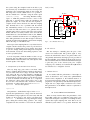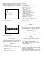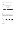
1
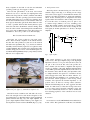
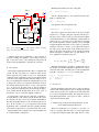
Free and Open Source Software for Industrial Process Control Systems Simone Mannori , Ramine Nikoukhah , Serge Steer INRIA-Rocquencourt, Domaine de Voluceau, 78153 Le Chesnay Cedex, France [email protected] , [email protected], Abstract— Scilab and Scicos are open-source and free software packages for design, simulation and realization of industrial process control systems. They can be used as the center of an integrated platform for the complete development process, including running controller with real plant (ScicosHIL: Hardware In the Loop) and automatic code generation for real time embedded platforms (Linux, RTAI/RTAI-Lab, RTAIXML/J-RTAI-Lab). These tools are mature, working alternatives to closed source, proprietary solutions for educational, academic, research and industrial applications. We present, using a working example, a complete development chain, from the design tools to the automatic code generation of stand alone embedded control and user interface program. Keywords: Real time control; dynamical systems simulation; simulation software; hybrid systems; Scilab; Scicos; RTAI; Comedi. I. I NTRODUCTION We show, using a real example, a complete development chain that allow to: • • • • • • • construct a mathematical model of the plant; validate the model of the plant through simulation and open-loop measurements; design a suitable controller; simulate the full system and optimize controller parameters; run the controller inside the standard simulator while connected to the real plant in ”soft real-time” mode (SCICOS-HIL: Scicos Hardware In the Loop); use an automatic code generator to create stand-alone controller program that could run stand alone in ”hardreal-time” mode (Linux-RTAI Code Generator; implement graphics user interfaces (RTAI-Lab, J-RTAILab) to remotely interact with the controller using network connections. We provide all the references to the documentation, available thought Internet, that describe all the details of installation, configuration and utilization of the software packages involved. Our aim is just to show what is possible to realize within a very limited budget: we try to limit [email protected] the cost of the parts using standard, low cost devices and stimulate development of solutions that use imagination instead of money. Just as an example, the cost of all the software used is zero. II. S OFTWARE PACKAGES OVERVIEW One - if not the most important - critical issue for the developing of modern digital control systems are the software tools used for the design and validation. A. Scilab We use Scilab/Scicos as main development environment. Scilab [1] is a scientific software package for numerical computations providing a powerful open computing environment for engineering and scientific applications. Scilab has a complete functions toolbox for modeling, simulating and aiding the design of hybrid control systems. Since 1994 it has been distributed freely along with the source code via the Internet. It is currently used in educational and industrial environments around the world. Scilab includes hundreds of mathematical functions with the possibility to add interactively programs from various languages (FORTRAN, C, C++, JAVA). It has sophisticated data structures (including lists, polynomials, rational functions, linear systems), an interpreter and a high level programming language (Scilab Language). B. Scicos Writing the simulation of an hybrid dynamical system as scripts, using the powerful functions of the Scilab language is possible [2], but it is time consuming and it is very easy to insert bugs during the manual coding. To simplify this job, Scilab include Scicos [3] a graphical hybrid dynamical system modeler and simulator toolbox. Scicos is used for applications in control system, communication, signal processing, queuing systems, and to study physical and biological systems. Within Scicos graphical editor it is possible to place, configure and connect blocks, in order to create diagrams to model hybrid dynamical systems, and simulate it. Most of the Scicos graphical user interface is written in Scilab language, for complete integration with Scilab, easy customization and maximum flexibility. Each blocks is rapresented by two functions: • • the interfacing function. Written in Scilab language, define the graphical representation, the input, output and control ports and signals and the user configurable parameters ; the computational function, that is the real code used in the simulations. The computational function can be written in Scilab Language, for easy development, or in C, for maximum efficiency and speed. The C computational function can be pre-compiled or ”compiledbefore-simulation” in order to allow the user to ccustomize without leave the Scicos environment. Scicos simulations could be used to interact with real system in many ways: • • • Scicos HIL (Hardware In the Loop). With some limitation is possible use the Scicos simulation to control a real plant in real time. the internal, general purpose, C generator. The internal ”Code Generator” (menu ”Object”-¿”Code generation”, [4] ) translate the Scicos symbolic diagram representation in stand alone, general purpose C code. This code uses the standard I/O (terminal) as interface. It is left to the user to customize the C code in order to interact with other input/output devices (e.g. data acquisition cards) and resolves the real time and synchronism issues. This basic, but very flexible solution, is designed to work with hand coding or with external software tools as Syndex[5]. For the next release of Scilab (vers. 5) the internal code generator will be fully integrated with Syndex to allow the physical implementation of Scicos diagram on multiprocessors and programmable logic architectures. use a specific code generator for Linux RTAI. This solution merge the hard real time capability of LinuxRTAI kernel [6] with the creation of a stand alone program from Scicos computational functions, ideal for embedded systems with limited hardware resources. The stand alone program that implement the Scicos diagram con exchange data using the RTAI-Lab user interface or the J-RTAI-Lab user interfaces. The former needs RTAI installed in the host system, the latter uses Java applets that runs on any Java enabled browser on any OS. C. RTAI-Lab user interface RTAI-Lab is a graphics environment that allow to display, in real time, the internal variables of a RTAI running controller, using scopes and other virtual instruments. It is also possible modify the internal parameter in order to tune the system. RTAI tasks and RTAI-Lab exchange data using IP address and NET-RPC protocol. The NETRPC uses Ethernet (or other compatible media/interfaces) in real time using custom UDP data packet. This protocol support an arbitrary number to tasks/controller connected with a single supervisor. This is the ideal environment for distributed control applications. With some limitations on the network load, the same media can support real time and standard TCP/IP connection simultaneously. RTAI-Lab uses RTAI API to synchronize the communication and update the display with real time priority. This imply the presence of an Linux RTAI also in the supervisor PC that run RTAILab. It is possible to avoid this requirement: the RTAIXML/J-RTAI-Lab [7] allow to use a general purpose Java enabled web browser to implement the same features of RTAI-Lab but without any garantee about the latency of the data exchange. D. Comedi device drivers and libreries Comedi [8] is the standard way to use I/O interface devices with Linux. The Comedi project develops open-source drivers, tools, and libraries for data acquisition. Comedi is a collection of drivers for a variety of common data acquisition plug-in boards (more than 100 devices are supported). The drivers are implemented as a core Linux kernel module providing common functionality and individual low-level driver modules. To use the driver, the application program should use Comedilib functions. Comedilib is a user-space library that provides a developer-friendly interface to Comedi devices. Included in the Comedilib distribution is documentation, configuration and calibration utilities, and demonstration programs. Kcomedilib is a Linux kernel module (distributed with Comedi) that provides the same interface as Comedilib in kernel space, suitable for real-time tasks. It is effectively a ”kernel library” for using Comedi from realtime tasks. This is a very important features because the hard real time RTAI tasks could not issues direct system call to uses. E. Linux and RTAI-Linux kernels The Linux kernel is the foundation over all this building is constructed. The Linux kernel provides a level of flexibility and reliability simply impossible to achieve with any other (free or commercial) operating system. For these reasons, many companies in the field of real time and embedded operating systems [9] offer support for Linux. The real time performances of the latest 2.6.1x Linux kernel are very close to real time (for sampling time in the milliseconds range) but the ”vanilla” (standard, unmodified) Linux is NOT a real time operating system because with the standard Linux kernel is not possible give guarantee about the absolute maximum latency of task activation. There are many project that modify (patch) the Linux kernel in order to create a ”parallel” hard real time kernel (and user) space where the tasks have deterministic activation timing, while leave the other ”normal” tasks running in the standard Linux user’s space. We use RTAI because offer direct support for Scilab/Scicos, but is also possible to use Xenomai [10]. III. C ONSTRUCTION A. Ball position sensor The ball position is measured using one of the rails as a variable voltage source (Fig. 3). A floating 5 Volts voltage and a series resistor, supply a constant 700 mA current to the reference rail. This arrangements is simple but inefficient: almost all the electrical power is dissipated in the linear regulator and in the external 6.8 ohm / 5 Watt power resistor. To avoid this waste of electrical power, we plan to use a constant voltage (100mV ), low noise, switching power supply. The metallic (stainless steel) ball works as a sliding contact; the second rail closes the circuit, sending the low level signal (0 − 40 mV, equivalent to 0 − 30 cm) to the input amplifier. LF 356 12K OF THE PLANT The fastest way to have a plant is to buy such ”readymade”. There are many companies on the educational market that offer such products [11]. We choose the classical ball and beam experiment (Fig. 1 (a)) because its intrinsic instability and non linearity represents a recognized control system benchmark. The construction is possible using readily available cheap parts. For most of the mechanical parts we use LEGO Technique/Mindstorm [11] components (less than 200 euro for a complete kit). Fig. 1. Complete system. From the bottom: (a) ball and beam; (b) amplifiers and power supplies; (c) USB-DUX data acquisition card. The ball is made of stainless steel. The ball rolls on two brass rails salvaged from a train model and glued on the Lego bricks (Fig. 1(a)). We build, using a single experimental printed circuit board (Fig. 1(b)), the input amplifier, the power output amplifier and the relatives power supplies. As data acquisition cards we use the USB-DUX (Fig. 1(c), [13]). Rs E + − 0.47uF 5 Volt − Fig. 2. R 6.8 120 + 0 − 40 mV C Ro 330K+270K R1 10K R2 0 − 2 Volt L_beam = 30 cm Input Amplifier. The contact resistance is very noisy (typical moving contact noise). The input amplifier (Fig. 3) has high-input impedance and uses a low pass filter (R and C) that cut out part of the noise from this sensor. We provides two time constants (5ms and 0.5ms) compatible with expected closed loop dynamic of the plant. With the high-impedance of the JFET operational amplifier LF356, if the ball loose the electrical contact with the rail(s), the input filter works as ”sample-and-hold”: the capacitor C ”remember” the last valid voltage/position value. This non linear behavior of a fully linear filter and amplifier is an ”collateral effect” of the non-linear, random proprieties of the moving contact resistance, that represent the internal impedance of our position sensor. To have two moving contact (referencerail/ball and ball/sensing-rail) in series aggravate the final results. A common cure to reduce the moving contact noise is to use carbon based (electrical conducting) grease. We don’t use it intentionally because we want to evaluate the noise-rejecting proprieties of the controllers in worst cases situations. B. Actuator For actuator we use the LEGO Mindstorm standard motor model ”71427”. The specifications of this motor are available [14] from experimental tests. The inductance of the motor’s armature (LA = 2.07mH, average value, measured with an impedance bridge) is not included in the model because it introduces a time constant τe = LA /RA = 0.83ms which can be neglected. The limited electromechanical conversion efficiency of the motors appears as different KT (torque constant) and KV (speed constant). These two constants are equals in the case of ”perfect” 100% efficient motor, where all the electrical power is converted in mechanical work. The constants are different also because inside the Lego motor there is a reduction gear that lower the efficiency but increase the torque (reducing the maximum speed) and improve the linearity of the DC motor in the low speed region. The estimated internal motor plus reduction gear equivalent moment inertia are negligible respect the the moment of inertia of ball and beam. In the model, we neglect all the other possible sources of friction. The motor has more than sufficient speed and torque to move the ball and the beam directly. We introduce an external reduction gear to utilize better the motor speed range. C. Power Amplifier The output of an operational amplifier is boosted with a complementary pair Darlington transistors. This linear power amplifier has more than sufficient bandwidth (10kHz), voltage (+/ − 15V ) and current (+/ − 1.5A) capability to drive the loaded motor. The output voltage is limited to +/ − 9V to avoid motor overload (that will permanently damage the motor). We choose to set AV = 1 for the power amplifier because we found that the +/ − 4V dynamic range of the USB-DUX output voltage is enough to drive the motor (the output amplifier works only as current booster with voltage gain set to one). D. Encoder Input Using the bidirectional counter input of the data acquisition card (USB-DUX) is possible to connect an encoder measuring the real angle of the beam. We have not used this input in the experiment because we choose to use an observer to recreate the full state of the system. With an observer, it is possible to avoid the necessity of an expensive sensor to measure the position of the beam. E. Data Acquisition Card We use the USB-DUX [13] interface. We choose this device because it has sufficient resources to monitor and drive the plant. USB-DUX uses a Universal Serial Bus connection: his allow to use any recent laptop. USB-DUX uses Comedi [8] device driver suite that allows to use different hardware without a coherent API. In the spirit of free and open-source development, the USB-DUX is fully documented (hardware and software), including schematics and source code of the firmware of the micro-controller that runs the board. The only real limit of this board is the USB bus: unfortunately it is not yet possible to run it in true hard-real-time fashion USB interfaces because, to do so, it is necessary to rewrite the full USB Linux stack [15]. Usually, with recent 2.6.1x kernel this is not a serious limitations for applications with sampling time of 10ms or higher. At present time, the only way that allow a full hard real time guarantee behavior, is the use of ISA/PCI/PC-CARD I/O board [7]. IV. M ODELLING AND S IMULATING THE S YSTEM A very useful way to evaluate all system constants is to write all the equations inside a single Scilab script ( bb 10.sce ; see appendix A). In the first part of the script all the system constants are defined; then these constants are used to calculate the coefficients of the linearized model of the system. A. Modelling the plant Supposing that the linear model of the plant is represented by the time continuous state matrix A , B , C et D ; the discrete (sampled time) model is obtained using the Scilab instruction sys_d = dscr(sys,Ts); where sys is the Scilab object that represent the linear system: sys = syslin(’c’,A,B,C,D); The A matrix has dimension 4 × 4 (the model has four state see the annexe), the matrix B is 4 × 1 (there is only an input: the motor voltage), C is 1 × 4 (the position of the ball is the only output) and D is null. The eigenvalue of the the A matrix show that the linearized model is unstable in the equilibrium point (there is an eigenvalue with positive real part). A full state feedback approach is used to stabilize the system. The feedback matrix F is calculated using LQR method, using Q and R values tuned experimentally. With the full, linearized, model of the plant bb_a num(z) den(z) sys = syslin(’c’,A,B,C,D); and the sampling time T s, the equivalent discrete time plant is computed with Motor_In −Ki + + S/H Ball and beam Nonlinear model Ball_Position SUM = dscr(sys,Ts); and splitted in the four elements with OssPosError + L Bd sys_d − [Ad,Bd,Cd,Dd] = abcd(sys_d); SUM + + + 1/z Cd SUM Ad F Osserv Fig. 3. Scicos diagram bb a.cos with complete, continuous non linear model of the plant and the linear discrete controller. Adjusting the R and Q parameters of the controller is possible to change the dynamics of the transient response. Fig. 3 show the results of the simulation using R and Q values found experimentally to stabilize the controller. B. The regulator The regulator implemented inside a PC is a sampled data system, but the real plant is a continuous time system. Various approach are possible: we choose to transform the continuous model of the plant a a discrete one and design the controller in the sampled domain. The first things to do is choose a sampling time. Usually the sampling time is chosen looking at the closed loop expected performances. If Tr is the desired 10-90 response time to a step of the reference T s = Tr/10 or less. In other words: at last ten sample in the rise time. The sampling time should be high enough to cover, within the Fs/2 Nyquist limit, all the ”fast” poles of the plant in order to avoid intersampling oscillation. It is important to check also the ”authority” (capability to act with efficacy) of the actuator present in the real system. In our plant, the Lego motor has a intrinsic bandwidth in the range 10-40 Hz, function of the load inertia. We choose Ts = 10 ms because is a good compromise between this requirement and is realizable with the available hardware and software components in soft and hard real time modes. Input amplifier, data acquisition and output amplifier can be considered fully ”transparent”. The classic approach at the design of the state variable regulator is to compute, using the expected controlled system, the position of the closed loop poles, then and compute a feedback matrix F to do that. Scilab has a function that do all the work (F = ppol(A, B, poles)). This kind of approach has several drawbacks. A better solution is to use an LQR designed feedback matrix that is more robust to parameters variations and allow to find a good compromise between the time reponse and the effort on the actuator. In order to improve the steady state accuracy of the system, an external discrete integrator is added in the loop. The matrix of our new ”augmented” feedback system are : Fi = F Ad Ki , Adi = −Cd Bd 0 , Bdi = 0 I With this arrangement is possible to compute the gain of the integrator Ki and the stabilizing feedback matrix F at the same time. The value of R and Q are found experimentally using R = 1 and Q = [ 1 1 1 1 1] as starting point. F_lqr_i = bb_dlqr(Adi,Bdi,Qi,R) F = -F_lqr_i(1:4) ; Ki = -F_lqr_i(5) ; ; C. The observer Instead that fill the plant with sensors, using a Luenberg observer. The added integrator does not change the design of the observer because it is external at the real plant, then we use the non augmented matrix. We design the observer using manual placement of real poles in order to obtain an observer faster than the plant. V. T ESTING THE CONTROLLER WITH THE REAL PLANT: S CICOS H ARDWARE I N THE L OOP With some limitations, it is possible to use Scicos to control a real plant. The first step is to create input blocks to acquire the feedback signal and output blocks to drive the system. Using the examples found in the Scicos [17] and Comedi [18] documentation we have developed the interfacing and computational functions that realize the I/O using Scicos blocks. Within Scicos it is possible to run the simulation in ”real-time” using the menu option [Simulate]->[Setup] and setting ”Realtime scaling” equal ”1”. With this parameter set Scicos ”wait” for the right time to read the inputs, make the calculations and update the outputs. It is clear that the time required to complete all the actions should be less than the sampling time. Normally this is not a problems with the modern PC. Unfortunately, Linux is not an hard real time OS: also with free CPU time there is no guarantee that the sampling time will be respected. The latest 2.6.1x Linux kernel, with the low latency features active and with the internal timer set to the maximum resolution (1ms, 1000Hz) could be considered real-time at 99% for a sampling time of 10ms. This performance is more than enough for laboratory applications with electromechanical systems where sampling time in the range of 4-20 milliseconds. The respect of the sampling time is a very critical issue for a digital controller because the position of poles and zeros are function of sampling time T s. If T s change, the position of pole-zero change, with potential dangerous consequence in the transient, steady state and stability proprieties of the closed loop hybrid system. It is also important to limit the number of Scicos scopes and traces: they uses CPU resources. Increasing the scope’s internal buffers reduces the CPU loads, at the expense of the real time update of the display. A. Compensation of the mechanical non linearity The very cheap Lego parts create a non linear ”sticky friction” (sticktion) that block the movement of the beam for very low values of the motor voltage. As result of this ”dead zone” effect, the motor is totally incapable of making the small movement to place the ball in the perfect equilibrium position with zero ball speed. We use a custom Scicos block to create an artificial non linearity that try to compensate the ”dead-zone” effect, using a fixed voltage ”step” to the motor in the correct direction. The ”dead-zone” canceling non-linearty is realized inside the block Mathematical Expression that uses the equation: sign(u1)*a+u1 The parameter a , defined in the script or in the Context , represent the equivalent motor voltage of the the dead zone (the minimum voltage required to move the beam). The full regulator is show in Fig. 4. We used a non linear block Saturation to limit the motor voltage during the starting phase; during the normal working operation , the voltage computed form the controller is ever below the saturation level (+/- 2V). bb_abn Comedi D/A Comedi D/A CH−0 Motor num(z) den(z) −Ki + Mathematical Expression + + − SUM Kr 0.97 + L Bd SUM Comedi A/D Comedi A/D CH−0 − SUM + + + 1/z Ball Cd SUM Ad Observ F Fig. 4. Scicos Hardware In the Loop . B. The observer The fists attempt to manually place the poles of the observer was unsuccessful. The position signal is noisy because the rail-ball-rail contact is not perfect. This noise, only partially attenuated by the single pole low pass filter of the input amplifier, create stability problems in the observer. After several trial and error iterations with different strategies to place the poles of the observer (real poles, complex conjugate poles, deadbeat), we found that the LQR method was effective also to design the observer. C. Kalman observer At not satisfied with the performances of the LQR observer, we had tried to use a steady state optimal Kalman observer. The computation of the feedback matrix L is more involved because the Scilab ”lqe” function require the preparation of an equivalent system that include input (state), output and cross (input-output) correlation noise sources. The performances of the Kalman observer is equivalent to the LQR observer. VI. S CICOS RTAI C ODE G ENERATOR There are many situation where the performance of the Scicos-HIL solution are not sufficient: if the plant is unstable with catastrophic consequence, for fast/high accuracy systems that require sampling time lower than 4 ms, for embedded system where is not possible install the full Scilab/Scicos package but a small, stand alone program that implement the controller is the only option. The previous diagram can reused, but but all the I/O block must be from the specific RTAI Scicos palette. 0.10 0.05 0.00 −0.05 −0.10 Fig. 5. + 0.0 1.5 3.0 4.5 6.0 7.5 9.0 10.5 12.0 13.5 15.0 Ball position (m), time (s). ANNEXE M ATHEMATICAL MODEL OF 2.50 0.00 mg sin(θ) = mẍ + Js φ̈/r −1.25 Fig. 6. THE PLANT The mathematical model of the mechanical system has three ”internal state”: the ball posizion x, the ball’s rotation angle φ, and the beam angle, θ. The equation relative to the ball dynamics is 1.25 −2.50 [6] RTAI [Online]. Available: http://www.rtai.org; Available: http://www.dti.supsi.ch/ bucher/scilab-howto.pdf . [7] RTAI-XML Project [Online]. Available: http://artist.dsi.unifi.it/rtaixml/. [8] Comedi [Online]. Available: http://www.comedi.org/. [9] Links to companies [Online]. Available: http://www.linuxdevices.com/ . [10] Xenomai [Online]. Available: http://www.xenomai.org/ . [11] Quanser [Online]. Available: http://www.quanser.com; TQ Education and Training Limited [Online]. Available: http://www.tq.com/. [12] LEGO Mindstorm [Online]. Available: http://mindstorms.lego.com/. [13] USB-DUX [Online]. Available: http://www.linux-usb-daq.co.uk/. [14] LEGO motor parameters [Online]. Available: http://www.philohome.com/motors/motorcomp.htm. [15] USB-RTAI stack: works in progress [Online]. Available: http://developer.berlios.de/projects/usb4rt . [16] PC-CARD DAS16/16-AO Measurement Computing [Online]. Available: www.measurementcomputing.com . [17] [2], cap.9 ”Scicos Blocks”). [18] Comedi/Comedilib Tutorial and User Manual ”comedilib.pdf”. Available: http://www.comedi.org/. where r is the ball radius (meter), m the ball mass (Kg) et Js = 2mr2 /5, the rotational moment of inertia. + 0.0 1.5 3.0 4.5 6.0 7.5 9.0 10.5 12.0 13.5 15.0 Motor voltage (Volt), time (s). Using the relation x = φr whit the hypothesis that the ball roll without slide, the dynamics of the ball is simplified to ẍ = 5g sin(θ)/7. VII. C ONCLUSION In this paper we have presented a full working system that will be used for the teaching of the industrial control. R EFERENCES [1] Scilab [Online]. Available: http://www.scilab.org/. [2] S. L. Campbell, J-Ph. Chancelier et R. Nikoukhah, Modeling and Simulation in Scilab/Scicos, Springer, 2005. [3] Scicos [Online]. Available: http:www.scicos.org. [4] [2], cap.12 ”Code Generation”). [5] Syndex [Online]. Available: http://www-rocq.inria.fr/syndex/. A second equation model the dynamics of the beam : T = −mg cos(θ)x + Jb θ̈ + mx2 θ̈ where T represent the torque on the beam’s axis. Using the simplified model of the motor (that don’t consider the inductance): TM = KT iA where TM is the motor torque (Nm), KT the torque constant (Nm/A), and iA the motor current (A). Introducing the cinematic ratio of the gears that couple the motor to the axis of the bean KC = 40/8 = ωM /ω = T /TM where ωM is the rotational speed of the motor axis ω = θ̇, and the motor equation is UM = RA iA + KV ωM , we obtain KC KT iA = −mg cos(θ)x + Jb θ̈ + mx2 θ̈ where iA = UM − KV ωM . RA Substituting ẋ par v, we obtain the complete model: KV KC2 KT mgx KC KT UM cos(θ) − ω+ 2 2 Jb + mx RA (Jb + mx ) RA (Jb + mx2 ) θ̇ = ω 5 g sin(θ), v̇ = 7 ẋ = v. ω̇ = The state of this system are: (ω0 , θ0 , v0 , x0 ) = (0, 0, 0, ∗) where ∗ is an arbitrary value. It is possible to stabilize the ball in a generic position. We examine in detail the case x0 = 0. Linearizing the model around the equilibrium state 0, we obtain an approximate linear model: ξ̇ = Aξ + Bu y = Cξ where K K2 K ω − VRACJ T b θ 1 ξ= v,A = 0 x 0 0 0 5 7g 0 0 0 0 1 mg Jb KC KT R J A0 b 0 ,B = 0 0 0 0 and u = UM . The matrix C is 0 0 0 1 . This linear model is used for the design of the regulator and the observer.