Download Modeller - Institute of Transportation Studies

Quadstone Paramics V4.2
Modeller User Guide
Quadstone Limited
Version No. 3.0
22/12/2003
Distribution Classification:
Public Distribution
Quadstone Paramics V4.2
Modeller User Guide
Paramics is a registered Trademark.
The contents of this document are the copyright of Quadstone Limited. All rights
reserved.
22/12/2003/3.0
16 Chester Street Edinburgh EH3 7RA Scotland
Telephone: +44 131 220 4491 Facsimile: +44 131 220 4492
http://www.paramics-online.com
Quadstone Paramics V4.2
Modeller User Guide
Project title:
Quadstone Paramics v4.1
Document title:
Modeller User Guide
Document Identifier:
rrb/pv4/rel01
Distribution Classification:
Public
Document history:
Personnel
Date
Summary
Version
Scott Aitken /
Richard Braidwood
22/12/2003
3rd draft
3.0
Approval List:
Scott Aitken / Richard Braidwood (Quadstone)
Distribution List:
Public Distribution
Document Ownership and Confidentiality:
This document and all ideas, methodologies, algorithms, design Notes, descriptive
software text, etc, contained within remain the sole property of Quadstone
Limited. This document or any subpart of its contents must not be distributed, in
whole or part and in any medium, to any third party not listed on the distribution
list provided above. Any non-Quadstone employee listed on the distribution list
provided above must seek the express permission of Quadstone before divulging
any details of the contents of this document in any way, through any medium, to
any third party not listed in the distribution list provide above for the document
and its contents.
Modeller User Guide
1
Quadstone Paramics V4.2
Before You Begin ................................................................................ 4
1.1 Introduction to Paramics ...................................................................... 4
1.2 Basic Concepts and Terms ................................................................... 4
1.3 Modeller Development Cycle................................................................. 5
1.4 How this Manual is Organised ............................................................... 5
1.4.1
Tutorial ..................................................................................... 6
1.5 Reference .......................................................................................... 6
1.6 Conventions used in this Manual ........................................................... 7
2
Tutorial.............................................................................................. 8
2.1
Introduction to the Tutorial .................................................................. 8
3
Introduction to Paramics Modeller ......................................................... 9
3.1 Modeller Start-up................................................................................ 9
3.1.1
Layout of Modeller Window .......................................................... 9
3.1.2
Dropdown Menus...................................................................... 11
3.1.3
Reporter Window ...................................................................... 12
3.1.4
Navigation ............................................................................... 12
3.1.4.1 Three Button Mouse ............................................................... 12
3.1.4.2 Mouse plus Navigator Panel..................................................... 13
3.1.4.3 Keypad HotKeys .................................................................... 13
3.2 Paramics Editor ................................................................................ 16
3.2.1
Adding a Link ........................................................................... 16
3.2.2
Node Editing ............................................................................ 17
3.2.3
Link Editing.............................................................................. 18
3.2.4
Zone Editing ............................................................................ 19
3.3 Exiting Paramics Modeller and Archiving .............................................. 21
4
Network Build I................................................................................. 22
4.1 Units ............................................................................................... 22
4.2 Model Area Template......................................................................... 23
4.3 Skeleton Network Coding ................................................................... 25
4.4 Urban Network Junction/Intersection Coding ........................................ 32
4.4.1
Priority Junction/Intersection ..................................................... 32
4.4.2
Traffic Signal Junction/Intersection ............................................. 36
4.4.3
Roundabout Junction/Intersection............................................... 38
4.4.4
Kerbs and Stop Lines ................................................................ 40
4.5 Infrastructure ................................................................................... 41
4.5.1
Annotation............................................................................... 41
5
Traffic Demand I............................................................................... 44
5.1 Zone Specification............................................................................. 44
5.1.1
Zone Areas .............................................................................. 44
5.2 Demand Specification ........................................................................ 46
5.2.1
Demand Editor ......................................................................... 47
5.2.2
Display Demands...................................................................... 48
5.2.3
Sector Editor and Displaying Sector Demands .............................. 48
5.3 Vehicles Specification ........................................................................ 49
5.3.1
Vehicle Characteristics .............................................................. 49
5.3.2
Vehicle Proportions ................................................................... 51
Quadstone Paramics V4.2
1
Quadstone Paramics V4.2
Modeller User Guide
5.4 Profile Specification ........................................................................... 52
5.5 Fixed Demand .................................................................................. 53
5.5.1
PT Routes ................................................................................ 54
5.6 Run Initialisation............................................................................... 55
5.7 Additional Exercises .......................................................................... 56
6
Traffic Assignment I .......................................................................... 61
6.1 Introduction ..................................................................................... 61
6.2 Network Coding ................................................................................ 61
6.2.1
Cost Factors............................................................................. 61
6.2.2
Category Cost Factors. .............................................................. 61
6.2.3
Link Cost Factors ...................................................................... 62
6.3 Model Parameters ............................................................................. 62
6.3.1
Generalised Cost Coefficients ..................................................... 62
6.4 Assignment Methods ......................................................................... 64
6.4.1
“All-or-nothing” Assignment....................................................... 64
6.4.1.1 Major/Minor Links .................................................................. 65
6.4.2
Stochastic................................................................................ 66
6.4.3
Dynamic Feedback.................................................................... 67
6.4.4
Combining Assignment Techniques ............................................. 67
7
Collecting & Analysing Model Results I ................................................. 68
7.1 Gathering Statistics........................................................................... 68
7.1.1
Statistics ................................................................................. 72
8
Network Build II ............................................................................... 74
8.1 Urban/Highway Network .................................................................... 74
8.1.1
Links with Medians.................................................................... 75
8.1.2
Curved Links ............................................................................ 76
8.1.3
Ramps and Slips....................................................................... 76
8.1.4
Node Bounding Box .................................................................. 79
8.2 Network Restrictions ......................................................................... 79
8.2.1
Turn Restrictions ...................................................................... 82
8.3 Infrastructure ................................................................................... 82
8.3.1
Loop Detectors ......................................................................... 82
8.3.2
Sign Posting............................................................................. 83
8.3.3
Lane Choices............................................................................ 84
9
Traffic Demand II.............................................................................. 88
9.1 Zone Specification............................................................................. 88
9.2 Parking............................................................................................ 90
9.3 Time Periods and Time Dependent Inputs ............................................ 95
9.3.1
Time Dependent Demand Files ................................................... 95
9.3.1.1 Time Dependent Profile File..................................................... 95
9.3.2
Time Dependent PT Files ........................................................... 99
9.3.3
Time Dependent Vehicles Files ................................................... 99
9.3.4
Time Dependent Network Files ................................................... 99
9.3.4.1 Traffic Signals ....................................................................... 99
9.3.5
Periodic Link Changes ..............................................................100
2
Quadstone Paramics V4.2
Modeller User Guide
Quadstone Paramics V4.2
9.4
Multiple Profiles ...............................................................................101
10
Traffic Assignment II ........................................................................105
10.1
10.1.1
10.2
10.2.1
10.2.2
10.3
10.4
10.5
10.6
11
Random Release of Vehicles .........................................................105
Modifying the Release of Traffic .................................................106
Features Affecting Traffic Routing .................................................107
Restrictions.............................................................................107
Forced Lane Changes ...............................................................108
Averaging Feedback Costs ...........................................................110
Additional Exercises ....................................................................113
Strategic Routes .........................................................................115
Generalised Cost Coefficient .........................................................116
Collecting & Analysing Model Results II...............................................118
11.1
Gathering Loop Detector Data ......................................................118
11.1.1
Generated Text Files ................................................................118
11.1.2
Interactive Detector Data .........................................................119
12
Index .............................................................................................120
Quadstone Paramics V4.2
3
Quadstone Paramics V4.2
1
1.1
Modeller User Guide
Before You Begin
Introduction to Paramics
Paramics is a suite of high performance software tools used to model the
movement and behaviour of individual vehicles on urban and highway road
networks.
The Paramics Project Suite consists of Paramics Modeller, Paramics Processor,
and Paramics Analyser.
Paramics Modeller provides a visualisation of road networks and traffic demands
using a graphical user interface (GUI). Geographic and travel data is input to the
program which then simulates the lane changing, gap acceptance and car
following behaviour for each vehicle. The speed of the simulation is governed by
the computer processing power, the size of the network and the number of
vehicles on the network at any one time.
Paramics Processor configures and runs the traffic simulation in batch mode
without visualisation of the network through the GUI. This dramatically increases
the speed of simulation and is used to collect simulation results for the numerous
test options and sensitivity tests required.
Paramics Analyser reads output from the simulation model and provides a GUI to
compare post processing simulation results to observed data and to contrast and
analyse different test results.
This User Guide concentrates on the Paramics Modeller tool and uses examples to
describe how the software can be used to build traffic models and extract
simulation results.
The Paramics software development
functionality being created to meet
developments in ITS or traffic planning
Modeller or on the contents of this
Paramics web site at:
is an ongoing process, with additional
customer needs or to match further
processes. If you have any comments on
User Guide, please access Quadstone’s
http://www.paramics-online.com
1.2
Basic Concepts and Terms
Modeller, requires two main inputs. The first is the road network data, the second
is the travel demand data.
Road network data consists of geometric layout, junction descriptions, lane
markings and turning movement information. Junction or intersection descriptions
are stored in the model as "node" data where each junction is allocated a node
number or name. The road network which connects between nodes, describes the
geometry of the road, the lane specification and the distance. The connection
between two nodes is called a "link".
The study area can be divided into sub-areas known as "zones" which may be
distinct geographical boundaries (e.g. rivers, railways, canals etc.), or socioeconomic boundaries (e.g. residential areas, industrial areas, shopping etc.) or
boundaries specific to local model conditions (e.g. to accommodate internal
screenlines). The travel demand is modelled as zone to zone movements and is
represented by an origin/destination matrix of trips.
4
Quadstone Paramics V4.2
Modeller User Guide
Quadstone Paramics V4.2
Zones within the study area are referred to as internal zones while zones outside
the study area are referred to as external zones.
The traffic assignment process allocates the journeys (or trips) to appropriate
routes through the network. Alternative routes are calculated depending on
perception of link costs, on network congestion and on network restrictions such
as banned turns.
Additional "fixed demands" such as service bus data can also be coded directly
onto the road network with pre-defined specified routes.
To ensure that the model reflects as accurately as possible the existing road
conditions, a "base year" model is usually constructed. The current road network
and travel demand patterns are modelled and compared to observed traffic data.
Where the comparisons are within acceptable guideline criteria (ref. DMRB Vol 12
Traffic Appraisal in Urban Areas) the model in considered to be calibrated and
validated.
The process of "calibration" allows for the adjustment of parameters used within
the model, fine-tuning the model output to give acceptable matches to observed
data. However, the results must be shown to be robust and consistent and any
changes to default parameters must be justifiable.
Model "validation" consists of independent checks of the calibrated model.
Observed independent data (not used for model calibration) is compared to model
output and verified against guideline criteria.
1.3
Modeller Development Cycle
The Modeller development cycle consists of the following seven steps:
1. Creating a new Paramics network and embedding an overlay file.
2. Constructing a road network by adding nodes, links and zones and coding
detailed lane and junction description.
3. Constructing demand matrices from origin/destination data, and including
fixed demand data such as PT Routes.
4. Assigning traffic using an appropriate assignment technique.
5. Collecting and analysing model results.
6. Calibrating base conditions by comparing model results to observed data
7. Validating the calibrated base model against independent data.
All stages of the network construction and simulation process require checking
and validation. Guidelines for good practice are published by the Department of
Transport (UK) in DMRB Vol 12: Traffic Appraisal in Urban Areas. Paramics users
are recommended to adhere to these practices or to similar national standards
when building traffic models.
1.4
How this Manual is Organised
This manual is primarily designed as a tutorial guide to enable user to be come
familiar with the core concepts of the Paramics Modeller software. Advanced User
guides covering areas such as the use of “3D”, “Junction Analysis”, “Cut and
Paste”, “Calibration”, “Incidents”, “Strategic Routing” and “VA Signals” are also
available as separate documents.
Quadstone Paramics V4.2
5
Quadstone Paramics V4.2
Modeller User Guide
1.4.1 Tutorial
Modeller is highly interactive and therefore easier to learn by building example
models to simulate traffic movements. New users are recommended to read the
tutorial section at their workstations and to complete the simple modelling
examples. The tutorial gives detailed instructions for the first five stages of the
development cycle: creating a new network, building the network, building
demand matrices, traffic assignment and collecting model results. The final
stages, model calibration and validation, can vary from model to model and may
be controlled by published guidelines. For example, in the UK the Department of
Transport recommends criteria for model building and validation. The user is
advised to follow these recommended criteria or use other national standards
where appropriate.
The tutorial is set out in sections corresponding to the development cycle stages,
with a first set of examples relating to urban network coding and a second to
highway network coding. There is a degree of overlap between these two stages
where the coding is applied to both urban and highway networks.
Knowledge of traffic modelling techniques and procedures is an advantage and
experienced traffic modellers should recognise and be familiar with a number of
the techniques used in Paramics Modeller. However, the programme's intuitive
nature means that all users should quickly become comfortable with the
development cycle for model building.
1.5
Reference
A full explanation of Modeller commands and a description of associated ASCII
output statistics files is contained in the Modeller Reference Manual.
6
Quadstone Paramics V4.2
Modeller User Guide
1.6
Quadstone Paramics V4.2
Conventions used in this Manual
1. Text to be typed at the keyboard is shown in the format:
type this exactly
2. Messages and ASCII files generated by Paramics are shown as follows:
Now using standard demands and zones files, network has also been
Saved/Refreshed.
3. Paramics filenames occur in the following bold text:
configuration
4. Paramics commands, selected by clicking with the mouse keys are shown in
bold text as follows:
File>>Edit
The >> shows the direction of sequence of the commands starting with the left
command. All commands to the right will be sub-commands of the previous
selected command.
5.Folder names are shown as italic bold
Training/urban
6. "Click" always means to use the mouse buttons. All mouse operations in this
User Guide assume that a 3 button mouse is installed.
Quadstone Paramics V4.2
7
Quadstone Paramics V4.2
2
Modeller User Guide
Tutorial
2.1
Introduction to the Tutorial
The tutorial section of this document includes the following chapters:
•
Introduction to Modeller
•
Network Build I
•
Traffic Demand I
•
Traffic Assignment I
•
Collecting and Analysing Model Results I
•
Network Build II
•
Traffic Demand II
•
Traffic Assignment II
•
Collecting and Analysing Model Results II.
It is intended that the user reads the tutorial at their workstation and follows the
step-by-step instructions to build simple models.
The model build procedure is divided into two sections. The first section
introduces basic model build techniques while the second section introduces
additional techniques together with some enhancements to the basic features. In
the process you will be introduced to all the major features of Paramics Modeller.
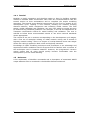
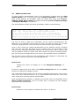
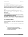
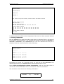
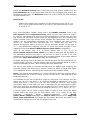
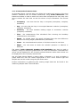
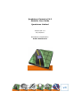
When the tutorial is completed, the Modeller window looks like Figure 1.
Figure 1: Completed Network
8
Quadstone Paramics V4.2
Modeller User Guide
3
3.1
Quadstone Paramics V4.2
Introduction to Paramics Modeller
Modeller Start-up
Modeller is available for a wide range of systems including Windows
NT/95/98/2000/XP Sun Microsystems/Solaris, Linux and Silicon Graphics/IRIX. To
install the software please refer to the instructions given in the Paramics Software
Installation Guide and ensure the toggle to load Modeller is selected. To run the
full version of Modeller a valid licence file is required.
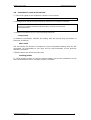
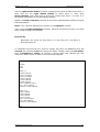
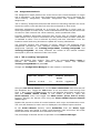
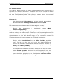
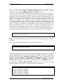
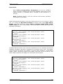
After installing the software a Modeller icon will appear on the monitor screen. To
start a Modeller simulation, double click on this icon using the left mouse
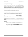
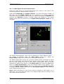
button. A display window appears similar to Figure 2 below.
If the software is loaded on a Unix workstation, simply type the command
“modeller &” in a shell window and press return. The display window will be
similar on PC and on Unix but with slight variations depending on the window
manager in use.
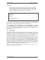
Figure 2: Screen Layout
3.1.1 Layout of Modeller Window
The Title Bar of the Main window displays the name of the current simulation
network and is positioned on the top of the Paramics Main window. The Menu Bar
is positioned immediately below the Title Bar and comprises of the Paramics
dropdown menus: File, Edit, View, Tools, Simulation and Help.
Quadstone Paramics V4.2
9
Quadstone Paramics V4.2
Modeller User Guide
Each menu choice is described in detail in the Modeller Reference Manual. The
Icons Toolbars, if selected, are displayed immediately below the Menu Bar and
comprises of the shortcut icons.
The Paramics Simulation window comprises of the network viewer. This is the
major part of the Paramics Modeller software and is used to pan and zoom
throughout the simulation network and is also the key to the editing via the
Graphical User Interfaces (GUIs).
Below the Simulation window the Network Editor Toolbar will be displayed if the
Editor Toolbar is initialised. The Reporter window is located immediately below
the Simulation window and is used to display messages and warnings to the user.
The Reporter window can be docked, undocked or hidden according to the users
preference.
Below the Reporter (from left to right) is the Progress Bar, Simulation Clock, Real
Time display, Vehicle display, Mode display and the Dimensional Mode display.
Around the edge of the Simulation window there is a dotted line that defines the
area for visualising simulated traffic, this is the Viewport (View>>Set
Viewport).
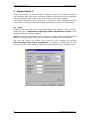
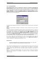
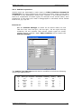
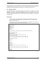
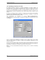
To open a new network select File>>New from the Menu Bar. The file browser
window allows the user to look at existing directories and select the required one
and selecting Open.
For example, to create a new network called Urban select File>>New. To name
this network simply select File>>Save as then select the directory location, in
this instance create a folder called Training, and type the name the network
Urban in the File Name field and select Save.
This opens a Modeller Main window for a new network called urban in the
directory called Training. In the urban sub-directory nine default files will be
created, namely, annotation, categories, demands, links, linktypes, nodes,
options, vehicles and zones. To view these files minimise the Modeller Main
window (click with left mouse button on the appropriate icon at top right of the
window) then use a text editor, such as Notepad, to open any of the eight default
files.
10
Quadstone Paramics V4.2
Modeller User Guide
Quadstone Paramics V4.2
Maximise the Modeller Main window (single click with the left mouse button
over the minimised icon). To increase the window size to full screen, click the left
mouse button on the small square icon at the top right of the Modeller Main
window.
The Modeller Main window shows a basic road network consisting of 4 nodes, 3
connecting links and 2 zones all within a simulation area. The simulation area is
marked as a dotted yellow rectangle inside the Simulation window.
An introduction to some of the Menu Bar choices and to a number of the Editor
Toolbar icons follows.
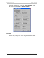
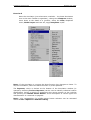
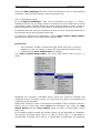
3.1.2 Dropdown Menus
By clicking with the left mouse key on Menu Bar choices (File, Edit, View, Tools,
Simulation etc.) dropdown menus appear. Each menu choice is described in
detail in the Modeller Reference Manual and the following simple example will
show the general selection procedure for these menus.
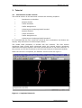
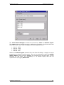
Preset an area by using the dropdown menu View>>Preset views>>Save
View>>0. The Paramics Input window appears showing a text box with the
prompt “Name for Preset View”. Click within the text block with the left mouse
button so that the text is activated and type a description such as “full network
view” and press OK.
This will return the Main window to the predefined area each time the 0 (zero)
key is pressed or when View>>Preset views>>Go To View>>full network
view is selected but only if the mouse arrow is within the Simulation window.
Quadstone Paramics V4.2
11
Quadstone Paramics V4.2
Modeller User Guide
3.1.3 Reporter Window
The Reporter window is “docked” just below the Simulation window, and its size
can be controlled using the adjustable pane control. The window displays warning
messages and it may be used to output information such as instantaneous data
on selected vehicles. If warning messages are displayed these should be read and
assessed to see if the warning is critical.
A standalone Status Report window can also be opened using Tools>>Reporter
(Crtl T) and this window can be dragged to any position on the screen.
3.1.4 Navigation
There are several different methods of navigating within the Modeller Simulation
window. The recommended method is to use the mouse buttons on a three
button mouse. Alternatively, use a mouse (one, two or three button) together
with the Navigator Control Panel or with keypad characters.
3.1.4.1 Three Button Mouse
Within the Simulation window, move the mouse arrow and click the left mouse
button to place the blue cross hair at the centre of the area of interest (“point
and click”). In addition to “point and click”, the left mouse can be held down
continuously as the mouse is “dragged” in the Simulation window. The position of
the view relative to the Simulation window changes. By releasing the left mouse
button the position is fixed at that point in the Simulation window (“drag and
drop”).
The “drag and drop” navigation is very sensitive and may therefore be difficult for
users who are not familiar with this technique. After some precise this is easily
mastered but to start it is probably advisable to use the “point and click”
technique.
By clicking the left and centre buttons simultaneously, the Simulation window
zooms out from the blue cross hair point (referred to as zoom up). The left and
right buttons clicked as the same time will zoom in toward the blue cross hair
(referred to as zoom down). While zooming up and down the blue cross hair
position remains fixed unless the Tools>>Options>>Zoom and Pan is toggled
on. With this option selected, the blue cross hair position can be dragged (i.e.
panning) around the Simulation window at the same time as the view is zoomed
up or down.
12
Quadstone Paramics V4.2
Modeller User Guide
Quadstone Paramics V4.2
3.1.4.2 Mouse plus Navigator Panel
The Navigator Panel can be toggled on or off using Tools>>Navigator.
If the Navigator Panel is displayed and the mouse arrow is positioned over the
navigator symbols, a tooltip appears briefly (only if Options>>Tooltips is
toggled on) on the screen. These tooltips describe the operation of each of the
symbols, for example, Pan Left, Pan Up, Zoom Down etc.. Clicking the left
mouse button (or single mouse button) on a symbol will perform the respective
operation within the Simulation window. For example, clicking on the symbol Pan
Left will reposition the blue cross hair to the left of its present position. The
incremental step can be changed using the + and – symbols to increase or
decrease the sensitivity.
The symbols Snap To, Select (Left) and Select (Right) are used for editing the
network and are described in the Modeller Editor section below.
3.1.4.3 Keypad HotKeys
A number of keypad characters have been defined as shortcuts (HotKeys) to
navigation operations and for display options. The navigation HotKeys are:
Tab
`
Right/Left/Up/Down Arrow keys
Ctrl with Right/Left/Up/Down Arrow keys
View Point Height Up
View Point Height Down
Focus Point (R/L/F/B)
Focus Point (R/L/F/B) (Fine)
If the mouse arrow is within the Simulation window area then pressing the
<Tab> key will zoom up while pressing the <`> key will zoom down. The
keypad arrow keys will pan the view in the Simulation window in each respective
direction.
Exercise 1
Use any of the methods described above to centre the blue cross hair
on Zone 1 and zoom down.
In the View dropdown menu click on model layers then the dotted
line to tear-off this menu. Toggle Zone Boundaries on and off by
clicking this option using the left mouse button.
Quadstone Paramics V4.2
13
Quadstone Paramics V4.2
Modeller User Guide
Toggle the navigator panel on/off using Tools>>Navigator. Toggle
the tooltips on/off using Tools>>Options>>Tooltips.
Exercise 2
Click on View>>Text and tear-off the menu for Node Names. Display
node names by clicking the left mouse to toggle Node Names on.
14
Quadstone Paramics V4.2
Modeller User Guide
Quadstone Paramics V4.2
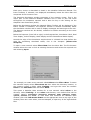
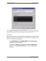
Click on Tools>>Display Settings then Text Sizes in the Display
Settings window and change the text height by clicking and holding
down the left mouse button to move the slider bar.
Click on Help>>Hotkeys to show shortcuts to toggling objects.
Quadstone Paramics V4.2
15
Quadstone Paramics V4.2
3.2
Modeller User Guide
Paramics Editor
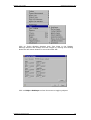
The Editor Toolbar is used to modify the network data dynamically. Editing can be
done at any time, even while the simulation is running.
There are four ways to open the editor. The first two use dropdown menus either
Edit>>Network or View>>Toolbars>>Edit. The third most commonly used
method is <Ctrl E>.
After opening the editor the Toolbar is conveniently located at the bottom of the
window.
Within the Editor Toolbar there are four function groups, namely; File Options,
Network, Demand and Modification. The File Options group contains the
save and refresh, refresh only, file editor, edit options and editor help.
Save and Refresh - the Save and Refresh function executes the
edits that have been made to the simulation network, saves the
changes and refreshes the screen display.
Note:- If any edits have been carried out but have not been saved then
no network changes are applied. Therefore, File>>Reload has the
effect of undoing any edits since the last Save and Refresh.
Refresh Only - the Refresh function will not save the network
changes but will refresh the screen while.
File Editor - the Edit function enables edits to be carried out directly to
Paramics files. This is useful for editing user specified files such as
demands, categories, profiles etc.
Editor Options – See Modeller Reference Manual for detailed
information on Cut & Paste, Scope, Periodic and Options menus.
Editor Help -. See Modeller Reference Manual for detailed information
on this menu.
The edit functions are contained within the Network and Modification groups. By
clicking on the icon within these groups specific functions can be undertaken.
The following section concentrates on editing the main network components i.e.
nodes, links and zones.
3.2.1 Adding a Link
Open the Editor Toolbar and click on Edit Nodes then using the left mouse
button select the location of the first node and select Add Node. Select the
location of the second node and select Add Node.
Next select a node using the middle mouse button, when selected the node will
be highlighted purple. Select the second node, this time using the right mouse
button, the second node will be highlighted as green.
Finally, select Add Link, this will launch the Link Attributes window enabling
the user to select the relevant link category.
Note:- Categories are explained in greater in Chapter 4.
16
Quadstone Paramics V4.2
Modeller User Guide
Quadstone Paramics V4.2
3.2.2 Node Editing
Open the Editor Toolbar and click on the Edit Node. In the Modeller Simulation
window zoom down to a node and using the middle mouse button click on the
node.
Note:- The modify Toolbar icons; add node, modify node, delete node and modify
junction become highlighted.
Using a two button mouse a selection is activated by clicking both buttons
simultaneously. Alternatively, in the Navigator Panel click on the symbol Select
(Middle) to select the node which is closest to the blue cross hair position in the
Simulation window.
Next select another node, this time using the right mouse button (similar for
two button mouse) or using Select (Right) from the Navigator Panel. Also, the
first node is highlighted as purple while the second node is highlighted as green.
Note:- It is important to be aware that a convention exists where the direction of
a link is always from first node to second node i.e. from purple to green.
Next click on Add Node.
Note:- If the purple and green nodes were at opposite ends of the same link then
the link would be highlighted as grey and the new added node would appear
halfway along the link. If the purple and green nodes were on different links then
the new node appears at the blue cross hair position. The new node becomes the
purple node. A node that is not connected to the rest of the network will be
highlighted as red.
A node highlighted as purple, is moved by holding down the <shift> key and
either clicking the middle mouse button to reposition the node at the blue cross
hair or by holding both keys simultaneously to drag the node around the screen.
The same functionality is achieved using the Snap To symbol on the Navigator
Panel.
After repositioning the node, select the Save and Refresh icon from the save
function group.
Quadstone Paramics V4.2
17
Quadstone Paramics V4.2
Modeller User Guide
3.2.3 Link Editing
In the Editor Toolbar window select the Link icon (as opposed to Node in the
above section). Select a link by moving the arrow to the required link and clicking
the middle mouse button (alternatively use Select (Middle) from the Navigator
Panel). The edit group keys should read Modify Link, Delete Link, Annotate
Link and Clear All.
Note:- Clicking on Clear All deselects everything.
Select the Modify Link icon to open a new window called Link Attributes. Drag
this window to a convenient position.
The link attributes of category, speed, width and lanes are automatically shown.
To view more link information select one of the following menus; Flags, Devices,
Link Modifiers and Category Info.
Use the slider bars to change the category, the speed, the width and number of
lanes by clicking and holding down the left mouse key to drag the slider bar.
These attributes can also be changed by single clicking the left mouse button
inside the grey slider bar windows.
Make a change to speed, width or lanes and click Apply. The changes can be
included in the network using the Save and Refresh button.
18
Quadstone Paramics V4.2
Modeller User Guide
Quadstone Paramics V4.2
An alternative way to select a link is to use the Node function to highlight nodes
at either end of a link. Select a node at one end of the required link using the
middle mouse button (or in the Navigator Panel click on the symbol Select
(Middle). Then select the node at the other end of the required link using the
right mouse button (or in the Navigator Panel click on the symbol Select
(Right)). Remember that the node selected using the Navigator Control Panel will
be the one closest to the blue cross hair position shown in the Simulation window.
Exercise 3
Use both the Node and Link functions to include crossroads and Tjunctions in the network. Save and Refresh changes.
To add a new junction on an existing link, the user is required to
firstly select the link and then using the node icon in the editor menu,
select the Add Node icon. As described previously the new node is
added at the mid-point of the selected link.
3.2.4 Zone Editing
Select the function Edit Zones icon from the Demands Toolbar and immediately
a green dotted rectangle appears in the Modeller Simulation window. The
rectangle defines the area of a new zone if one is added to the network.
By clicking with the middle mouse button in the middle of an existing zone, all
vertices of the bounding area of the zone are highlighted. If all the vertices of the
zone are marked then the entire zone can be dragged and moved around the
screen using the <shift> key together with the middle mouse button. The same
functionality can be achieved using the Select (Middle) and Snap To symbols from
the Navigator Panel.
To move an individual vertex, use the middle mouse button to click inside the
zone close to the required vertex and move it using the <shift> key and middle
mouse button.
Vertices can be added around the perimeter of the zone. New vertices are shown
as a small green dotted square. If a vertex is deleted the unconnected vertices of
the zone are automatically joined after Save and Refresh.
Exercise 4
Add new zones and position these so that the zone boundary covers a
link. Save and Refresh changes.
Quadstone Paramics V4.2
19
Quadstone Paramics V4.2
Modeller User Guide
Exercise 5
Start the simulation (two alternative methods – the Start Simulation
icon in the main Toolbar or spacebar); change the Viewport window;
zoom down to the detail of a junction; select the View dropdown
menu, Model Layers and tear off; toggle Stoplines on/off.
Note:- If the simulation is running the Start function key changes to Pause. To
stop the simulation, select the Pause function or press spacebar.
The Reporter, which is docked at the bottom of the Simulation window (or
opened by selecting Tools>>Reporter) can be used to identify individual vehicle
specification. Select a vehicle by positioning the mouse pointer on the vehicles
and pressing the middle mouse button. A full description of vehicle types and
characteristics in contained on page 49.
Note:- V3.0 compatibility for middle-mouse button selection can be activated
within Tools>>Options>>Vehicle Picking.
20
Quadstone Paramics V4.2
Modeller User Guide
3.3
Quadstone Paramics V4.2
Exiting Paramics Modeller and Archiving
There are two ways to quit the Modeller program. The first is dropdown menu
File>>Exit that also allows the user to save snapshots at that point in the
simulation and to save the preferred options (e.g. to show Zone Boundaries
etc.).
The second method is to press the <escape> key. This automatically quits
Modeller and saves the options selected at the instant of quitting the program.
Warning: It is important to note that if changes have been made to the
network without applying Save and Refresh then all changes will be
lost.
Exercise 6
Quit Modeller and then re-open from the Modeller icon to see the
network changes that have been saved.
Use the simulation mode icon to change the mode to single step
simulation. Run the simulation in single step mode.
Note:- The simulation clock has return to the value set as default.
This default simulation start time can be reset to the users
requirements in Edit>>Configuration>>Base Parameters.
The user may wish to archive material after a specific part of work has been
completed. To do this select File>>Archive>>Backup and include comments in
the box provide e.g. “Changed signal plan at High St / Church St junction”.
Modeller will archive the data after the user has selected the Backup function.
To restore archived data use File>>Archive>>Restore.
Note:- Restore will overwrite the network data that exists currently so be careful
when restoring from archives that work that has been done is not overwritten. It
may be that the user would prefer to use File>>Save As in the Editor Toolbar,
to save different stages of the network development in separate directories.
Alternatively, use the File>>Save As PRM option in the Editor Toolbar window.
This option saves the current network as a file with “.prm” filename extension, so
that all the network description files are contained in one “PRM” file as opposed to
a directory. To load this information the user selects the option File>>Open,
types the “PRM” filename in the selection box and selects OK (See Appendix A of
the Modeller Reference Manual - Paramics File System).
Note:- The backup function on the PC will require the Windows operating system
to show file extensions for known file types. To change this use the Windows
Explorer program or open the ‘My Computer’ folder. Select the View>>Options…
from the dropdown menu and select the View tab. Ensuring that the ‘Hide file
extensions for known file types’ is toggled off.
Quadstone Paramics V4.2
21
Quadstone Paramics V4.2
4
Modeller User Guide
Network Build I
Prior to this stage it is essential that a modelling overview has been completed
and decisions have been taken regarding modelling objectives and requirements.
This is generally known as the scope of the study or the scoping phase.
This tutorial assumes that an overview or scope has been completed and the
model area, model time periods and data requirements have all been identified.
4.1
Units
Paramics has three options for displaying speed and distance units, for more
details see the Configuration Manager>>Base Parameters>>Units in the
Modeller Reference Manual, page 22.
Note:- All internal calculations are carried out in metric units therefore minimal
conversion and rounding errors can be expected if imperial units are applied.
The user can define the default units used for each network by selecting
File>>Configuration>>Base parameters. In addition to specifying the units
the user can also select whether networks are right hand drive or left hand drive.
22
Quadstone Paramics V4.2
Modeller User Guide
Quadstone Paramics V4.2
Select Tools>>Grid and then 100m if using UK mode or 100ft if in US mode.
Then click the edit link icon and select any link by clicking on the link with the
middle mouse button. Using Modify Link note the link attributes of category,
speed, width and lanes. For UK mode the speed is in miles per hour and the width
is in metres. For US mode the speed is miles per hour and the width is in feet. To
switch between the modes select Edit>>Configuration>>Base Parameters
from the main menu bar and select US Units, UK Units or Metric Units from the
Units combo list. The grid automatically changes between 100ft squares and
100m squares. If you select the same link and Modify Link you see that the
speed remains in miles per hour but the width has changed from metres to feet
or visa versa.
4.2
Model Area Template
Detailed road layout plans can be read directly into Paramics and used as a
template to build the model road network. This removes the need to measure
road geometry manually from plans or from site measurements.
Overlays may be used as a template to build a network model. These can be read
into Modeller as Bitmap (bmp), AutoCAD (dxf) of TGA (tga).
For the purposes of this tutorial an AutoCAD file called overlay.dxf has been
prepared.
Exercise 7
Copy the file overlay.dxf from the media provided (either CD or
Floppy Disk) into the training tutorial directory i.e. Training/urban
Open the Training/urban network by clicking the Modeller icon and
selecting File>> Open (this is the network which was created in the
section Layout of Modeller Window on page 9).
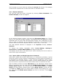
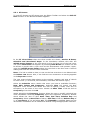
Load the overlay file by selecting Edit>>Overlays or the Overlay
Manager icon.
Quadstone Paramics V4.2
23
Quadstone Paramics V4.2
Modeller User Guide
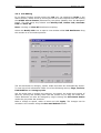
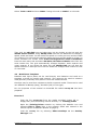
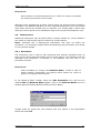
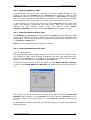
This will launch the Overlay Manager window that will allow you to manage
your overlay(s) within a network. Click the ‘Add’ button to select an overly file to
load for display. The file selector will be shown with the default BMP file filter,
change this to dxf. To select a file you navigate to the correct directory icon the
left panel and select the overlay file on the right panel. The restrictions on overlay
size and dimensions for raster images introduced in V3 remain in V4.
Once the overlay is loaded you can select the entry from the list and position the
associated overlay in the Paramics 3D world. The selected overlay will be
highlighted in the simulation graphics window in pink. The Position tab for
overlays enables the user to translate, scale and rotate the overlay in 3D.
Selecting OK commits your changes to file; Cancel discards any changes.
Note:- When nodes are added to the network, or existing nodes are re-positioned
the overlay data may need to be reloaded and repositioned. This is due to a nonlinier correlation existing between the physical position of nodes and the visual
position presented in the 3D Paramics world. This process is necessary to enable
3D graphics.
To avoid this it’s best to use a full Save and Refresh each time you add a new
node to the network while you are using background overlays to aid placement.
24
Quadstone Paramics V4.2
Modeller User Guide
Quadstone Paramics V4.2
It is recommended when coding a new network, using a background overlay, to
first position all the key nodes in the network, mapping out the extents of the
network before concentrating on the detail and the nodes towards the centre.
This will help reduce the potential for physical/visual mismatches in the 3D
coordinates.
Exercise 8
Using the Translation, Scaling and Rotation functions, found in
Edit>>Overlay>>Position, match the overlay grids to the Modeller
Simulation window grids. To help in differentiating between the
overlay grid and the Modeller grid, change the colour of the Modeller
grid using Edit>>Overlays>>Options>>Colour.
4.3
Skeleton Network Coding
A skeleton network defines the position of the main nodes and links in the model.
Before starting to code the skeleton network the user should define units and
preferences (refer to Exercise 7).
Match the location of the nodes to the junctions/intersections shown in the
overlay. Open the Editor Toolbar and selecting the Node icon then select a node
by moving the mouse arrow into the Simulation window and selecting the middle
mouse button. The node closest to the mouse arrow position will be highlighted
in purple. To move the position of the node hold down the <shift> key and press
the centre mouse key at the same time.
Note:- The node position will change to the point where the mouse arrow is
currently positioned. Alternatively, drag the node position by holding down the
<shift> key together with the middle mouse button and moving the mouse
position around the Simulation window.
New nodes and links should be added using the methods described on page 16.
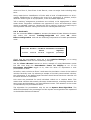
Initially make all links category 1 and ensure that the node positions match the
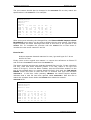
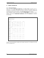
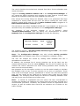
overlay junction/intersection positions. The resulting network should then be
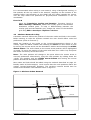
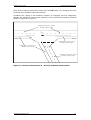
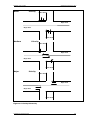
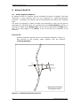
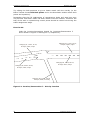
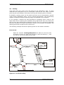
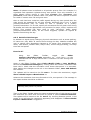
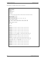
similar to the skeleton road network shown in Figure 3.
Figure 3 : Skeleton Urban Network
Church Street
Jnt. C
Jnt. D
Jnt. A
High Street
Mayfair
Park Lane
Jnt. B
Kelly Lane
Quadstone Paramics V4.2
Jnt. E
25
Quadstone Paramics V4.2
Modeller User Guide
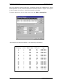
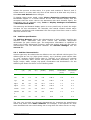
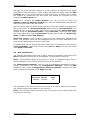
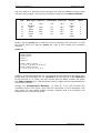
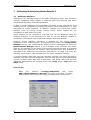
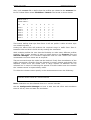
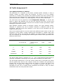
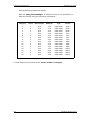
Once the skeleton network has been completed change the categories to match
those specified in the junction/intersection sketches shown in Figure 4 to Figure
8. At this stage do not try to match the speeds and widths.
To match categories use the drop down menu bar Edit>>Categories.
and change the categories based on the following information:
26
Category
Lanes
Speed (mph)
Width (m)
Type
1
2
3
4
1
2
3
4
30.0
30.0
30.0
30.0
3.7
7.3
11.0
14.0
urban minor
urban minor
urban minor
urban minor
5
6
7
8
1
2
3
4
40.0
40.0
40.0
40.0
3.7
7.3
11.0
14.0
urban minor
urban minor
urban minor
urban minor
21
22
23
24
1
2
3
4
30.0
30.0
30.0
30.0
3.7
7.3
11.0
14.0
urban major
urban major
urban major
urban major
25
26
27
28
1
2
3
4
40.0
40.0
40.0
40.0
3.7
7.3
11.0
14.0
urban major
urban major
urban major
urban major
Quadstone Paramics V4.2
Modeller User Guide
Quadstone Paramics V4.2
After all the changes have been made click the OK button. The changes will then
be saved and reloaded within the network.
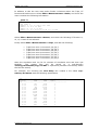
Complete the coding of the skeleton network by changing the link categories,
speeds and widths to match those specified in the junction/intersection sketches
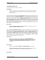
shown in Figure 4 to Figure 8.
Category 22, 2 lane, 24.0 ft,
30 mph, urban, m ajor
Category 21, 1 lane, 12.1 ft,
30 mph, urban, major
Category 21, 1 lane, 13.1 ft,
30 mph, urban, major
Category 22, 2 lane, 24.0 ft,
30 mph, urban, major
Figure 4: Junction/Intersection A – Priority Junction/Intersection
Quadstone Paramics V4.2
27
Quadstone Paramics V4.2
Modeller User Guide
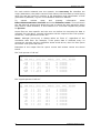
Category 22, 2 lane, 24.0
30 mph, urban,
Category 21, 1 lane, 13.1
30 mph, urban,
P1
P3
P2 P1
Category 21, 1 lane, 12.1 ft, 20
urban, major, wide
Category 22, 2 lane, 24.0
20 mph, urban,
Phase Diagram
Phase 1
Actual Green Time 20s
Red Time 0s
Phase 2
Actual Green Time 10s
Red Time 5s
Phase 3
Actual Green Time 20s
Red Time 5s
Figure 5 Junction/Intersection B – Traffic Signals
28
Quadstone Paramics V4.2
Modeller User Guide
Quadstone Paramics V4.2
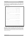
Category 22, 2 lane, 24.0 ft,
30 mph, urban, major
Category 21, 1 lane, 12.1 ft,
30 mph, urban, major
RB
Category 21, 1 lane, 12.1 ft,
30 mph, urban, major
Category 22, 2 lane, 24.0 ft,
30 mph, urban, major
RB
RB
Category 21, 1 lane, 13.1 ft,
30 mph, urban, major
Category 22, 2 lane, 24.0 ft,
30 mph, urban, major
RB
Category 22, 2 lane, 24.0 ft,
30 mph, urban, major
Category 21, 1 lane, 12.1 ft,
30 mph, urban, major
Figure 6: Junction/Intersection C – Roundabout
Quadstone Paramics V4.2
29
Quadstone Paramics V4.2
Modeller User Guide
Category 22, 2 lane,
30 mph, urban,
Category 22, 2 lane, 24.0
30 mph, urban,
Category 22, 2 lane, 24.0
30 mph, urban,
P1
P2
Category 21, 1 lane, 12.1
30 mph, urban,
Category 21, 1 lane, 12.1
30 mph, urban,
P2
P1
Category 22, 2 lane, 26.2
30 mph, urban,
Category 22, 2 lane, 24.0
30 mph, urban,
Phase Diagram
Phase 1
Actual Green Time 25s
Red Time 5s
Phase 2
Actual Green Time 15s
Red Time 5s
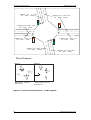
Figure 7: Junction/Intersection D – Traffic Signals
30
Quadstone Paramics V4.2
Modeller User Guide
Quadstone Paramics V4.2
Category 22, 2 lane,
30 mph, urban,
Category 22, 2 lane, 24.0
30 mph, urban,
P1 P2
Category 21, 1 lane, 12.1
30 mph, urban,
Category 22, 2 lane, 24.0
30 mph, urban,
P3
P3
Category 21, 1 lane, 12.1
20 mph, urban, major, wide
P2 P1
Category 21, 1 lane, 12.1
30 mph, urban,
Category 22, 2 lane, 24.0
30 mph, urban,
Phase Diagram
Phase 1
Actual Green Time 20s
Red Time 0s
Phase 2
Actual Green Time 5s
Red Time 5s
Phase 3
Actual Green Time 25s
Red Time 5s
Figure 8: Junction/Intersection E – Traffic Signals
Quadstone Paramics V4.2
31
Quadstone Paramics V4.2
Modeller User Guide
Edit the links using the Modify Link icon located on the Editor Toolbar. Select a
link by clicking in the Simulation window with the middle mouse button. For the
selected link, check the coding specified in Figure 4 to Figure 8 and use the
Modify Link function to re-code. For example, in Figure 5 Junction/Intersection B
the link from the west is defined as category 21, 1 lane, 12.1 ft, 20mph, urban,
major, wide start. By changing the category to 21 in the Link Attributes window,
the speed is automatically changed to 30 mph. This can be reset by dragging the
speed slider to 20 mph. To check the link is urban and to code a wide start select
the Flags menu and toggle the required buttons on.
Note:- The units displayed for speed and width will be the preferred units coded
within the Configuration Manager. Paramics converts all units to metric for
internal calculation and then applies conversion factors again to convert to US
Imperial measurements. The conversion of units can be subject to minimal
rounding errors and will not influence the simulation to any extent.
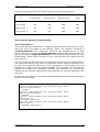
Check the coded widths for all links on the network and correct where necessary
(from the Editor Toolbar select Link and Modify Link as before).
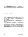
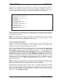
Again, in the Editor Toolbar select File Editor to activate the Paramics File Editor
window (See the Modeller Reference Manual page 108). Open the links file
selecting Network>>links. At the top of the Paramics Editor window the full
path
name
for
the
selected
file
is
displayed
e.g.
C:\Program
Files\Paramics\data\Training\urban\links. For some links the codes widths are
different from the default category widths and these are stored as individual
values in the links file.
4.4
Urban Network Junction/Intersection Coding
The aim for this section of the tutorial is to code examples of priority
junctions/intersections, roundabouts, and signalised junctions/intersections.
Figure 4 to Figure 8 should be used as reference for lane markings, turning
arrows and traffic signal plans.
4.4.1 Priority Junction/Intersection
Open the Editor Toolbar and select the node shown as Junction/Intersection A in
Figure 3. Refer to the junction/intersection details shown in Figure 4.
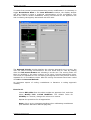
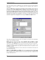
Select Modify Junction to open the Edit Junction window. The Edit Junction
window has five sections; Selected Priority, Signal Times, Turn Movements, Lane
Allocation, and Signal Display. The Cycle and Phases sections refer to signalised
junction/intersection and will be dealt with later in this tutorial.
32
Quadstone Paramics V4.2
Modeller User Guide
Quadstone Paramics V4.2
The Selected Priority section contains a skeleton diagram of the priority Tjunction/intersection with one movement highlighted with an orange arrow. Along
the orange arrow the priority associated with that turn is displayed in the priority
combo box. The priority may be MAJOR, MEDIUM, MINOR, or BARRED. To change
the priority select the new priority from the combo box and click OK.
The display in the turn movements tab will show colour changes to the specific
movement in the selected priority window (See Reference Manual page 79).
Note:- Highway links assume all priorities are major as this is one definition of
Highway links.
A hierarchy of priorities exists in the order of MAJOR, MEDIUM, MINOR and
BARRED. MAJOR priority movements are free flow and not restricted by other
streams of traffic (including major movements). A MEDIUM priority gives way
(yields) to MAJOR streams of traffic but has priority over MINOR traffic
movements. MINOR priority gives way to both MAJOR and MEDIUM traffic flows
while BARRED indicates the turn is banned to all vehicle movements.
Note:- Minor priority vehicles will slow down before proceeding even if no
conflicting movements exist.
To select a different turning movement click with the left mouse on the approach
arm of the turn required (within the diagram). Hold down the left mouse key and
move within the diagram area. The turn arrow switches towards the
junction/intersection arm closest to the mouse.
Quadstone Paramics V4.2
33
Quadstone Paramics V4.2
Modeller User Guide
Exercise 9
Edit the junction/intersection priorities so that turns from the southern
arm are MINOR i.e. give-way to all traffic; the left turn from east to
south is MEDIUM i.e. gives-way to oncoming traffic; and all other
turns are MAJOR. Save and Refresh all changes.
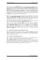
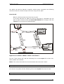
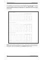
For reference, the following figure shows the recommended priority coding for a
four arm priority junction/intersection.
34
Quadstone Paramics V4.2
Modeller User Guide
Minor
Quadstone Paramics V4.2
Priority
Minor Arm
Major Arm
Major Arm
Minor Arm
Medium
Priority
Minor Arm
Major Arm
Major Arm
Minor Arm
Major
Priority
Minor Arm
Major Arm
Major Arm
Minor Arm
Figure 9: Priority Hierarchy
Quadstone Paramics V4.2
35
Quadstone Paramics V4.2
Modeller User Guide
4.4.2 Traffic Signal Junction/Intersection
Select the node shown as Junction/Intersection B in Figure 3 and refer to the
junction/intersection details shown in Figure 5.
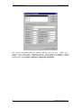
Again select Edit Node and Modify Junction icon from the Editor Toolbar. In
this case use the Signal Times tab. If a junction is a priority controlled
intersection then all functions are greyed out with the exception of Signalise. By
selecting the Signalise function a default signal plan appears in the Signal
Display section and all functions in the Signal Phasing/Signal Times tab are
activated.
The Signal Phasing/Signal Times can be displayed in three different ways. …
The display is selected using the View Style combo box. Select the
Group/Fixed display from View Style on the signal display tab.
The default signal plan shows red, green and amber/yellow rectangles to depict
the red, actual green and effective green phases of the traffic signal. The dark
blue box that borders one set of the green, amber/yellow and red boxes,
indicates the phase times shown in the Signal Times tab. Select the OK button
then click Save and Refresh to save the changes made to the network. Then,
using the middle mouse button, select the same node and Modify Junction.
To toggle between phases click with the left mouse button on the blocks of
green, amber/yellow and red.
Note:- Node descriptions in the Priority section changes to read Phase 1/2 or
Phase 2/2. The green and red times in the Phase Length will also change if the
two phase plans are different.
36
Quadstone Paramics V4.2
Modeller User Guide
Quadstone Paramics V4.2
A white line is also displayed in the Signals Display parallel to the Y axis. This
indicates the exact point the signal cycle plan is assumed to start. The position of
this line changes as the simulation runs in accordance with the simulated time.
The Phase Length section of the Signal Display window contains functions
enabling the user to modify the Green and Red time of individual phases. These
values can be modified by the user using arrow buttons located next to the
relevant attribute. The total time allocated to each phase and the overall cycle
times remain fixed if the Balance is set to This.
For Fixed Duration signals, modifications made to the red and green times of
the phase can to compensated for in the selected phase (Balance – This), in the
phase adjacent to the selected phase (Balance – Next) or across all phases
(Balance – All).
By default the amber/yellow time is set to 3 seconds and is automatically
displayed within the Signal Display. This can be toggled on/off using the Amber
check box in the Signal Times section. The 3 seconds is subtracted from the red
time if the red phase is 3 seconds or more.
Paramics assumes that the amber/yellow time is added to the actual green time
to give an effective green time. The user can choose to show the Effective or
Actual green time using the combo box within the Signal Times window.
Note:- The 3 seconds default amber/yellow time can also be modified to
represent local conditions within Edit>>Configuration>>Options.
Exercise 10
Change the cycle time by selecting Cycle Variable instead of Cycle
Fix in the Cycle Time section.
Note the cycle time changes by increasing or decreasing the Red or
Green times.
Code the traffic signal plan shown in Figure 5. Select the Signal
Display tab, click on the first phase and then click the Selected
Priority tab. Left click on the northern approach arm and select
Approach Barred from the Multiples combo box. Continue by
making the left turn from the west MEDIUM and all other turns
MAJOR. Using the Turn Movements tab check that all turning
movements have been allocated to the appropriate lanes (refer to
Figure 5).
In the Signal Times tab set the phase selected to phase 1. Then in
the Cycle Time section select Cycle Vary, toggle the Amber option off
and choose Actual. Then use the arrows beside Red to reduce the red
time to zero and on the Green time to set this to 20 seconds.
Repeat the process to code phase 2 and phase 3. Save and Refresh
when all changes have been completed.
The turn lane specification defines the lanes that different streams of traffic can
use on a link entering a junction/intersection. For example, if there is a
junction/intersection called Node B and you want to code the lanes for a turn A to
B to C, then the turning lane definition should show the lanes on link A:B which
the turn A to B to C can use.
Quadstone Paramics V4.2
37
Quadstone Paramics V4.2
Modeller User Guide
If link A:B has three lanes and only lane 2 is used for the turn A to B to C then
the Turn text box should read “2 – 2”. However if all lanes were permitted for the
turn then the coding should read “1 – 3”.
4.4.3 Roundabout Junction/Intersection
Select the roundabout identified in Figure 3 as Junction/Intersection C (in the
Editor Toolbar use Node icon and click with the middle mouse button on
Junction/Intersection E in the Simulation window). Refer to Figure 6 for link
category details.
In the Editor Toolbar window select Modify Node (not Modify Junction), the
Node Attribute Modifier window appears.
On the right hand side of this window there is a section headed New Roundabout.
Click with the left mouse button in the Diameter box and change to 15.0 m
(49.2 ft). Similarly change the Category to 22 and click on the Create function.
A roundabout will appear on the screen with the single node expanded to four
roundabout nodes (RB) with four roundabout sections.
The centre of the roundabout probably does not match exactly to the overlay. To
change the centre of the roundabout, choose the Edit Curves function from the
Editor Toolbar (the circle representing the centre of the roundabout is now
dotted). Edit Mode in the top left hand corner of the Paramics window tells you
the current curve editing mode. Select the square at the centre of the circle using
the middle mouse button and change the curve editing mode until this reads
Edit Mode: Fixed Radius by selecting the change curve mode function. Holding
the <shift> key and clicking with the middle mouse button, will reposition the
centre of the roundabout. Save and Refresh the changes.
The roundabout section links are all coded as category 22. Position the
roundabout nodes to match the overlay (marked as ‘RB’ positions in Figure 6)
using the Node function from the Editor Toolbar.
Edit the turning movements to be similar to the turn arrows shown in Figure 6.
This requires the user to modify all the roundabout nodes. Select node a
roundabout node and choose the Modify Junction
icon, then select the
Selected Priority window and Lane Allocation window within the Edit Node.
38
Quadstone Paramics V4.2
Modeller User Guide
Quadstone Paramics V4.2
To switch from normal junction/intersection priority modification it is necessary to
toggle Roundabout Data in the Lane Allocation window, the display window
will then change to show a graphical representation of the roundabout. This
allows the user to dictate roundabout turning movements for the approach link
and circulating carriageway associated with this node.
The Selected Priority window displays the relevant approach arm in green, the
user can select turning movements to the exit these wish to code by holding
down the left mouse button and releasing it at the exit. The turning lanes can
then be modified in the same manner as for other junction/intersection types.
This must be repeated for the circulating carriageway then the process must be
repeated for all roundabout nodes. After all turning movements have been coded
click OK and Save and Refresh.
An important aspect of coding roundabouts in Paramics is coding approach
visibility.
Exercise 11
Choose Edit Links from the editor toolbar an approach link, and then
select Modify Link >>Link Modifiers. The default value for
Visibility is 0 metres, change this value to 10 metres.
Repeat this procedure for all approaches.
Note:- this is a very important attribute when calibrating roundabouts
(See Modeller Reference Manual page 86).
Quadstone Paramics V4.2
39
Quadstone Paramics V4.2
Modeller User Guide
Exercise 12
Select and code the traffic signals shown in
Figure 7 and Figure 8 (Junctions/Intersections D and E, respectively).
4.4.4 Kerbs and Stop Lines
Kerbs and Stoplines can generally be described as ‘control points’ (See Modeller
Reference Manual page 91).
Each link has an inside and outside kerb point at the start of the link and at the
end (i.e. 4 kerb points per link, a pair of start kerb points and a pair of end kerb
points). By default, locus points (or control points) are defined along a line joining
each pair of kerbs so that for each lane on a link a locus point is drawn at the
centre of the lane. Vehicles have to pass through these locus points as they move
through a junction/intersection. For example, if locus points for the in and out
links of a 90 degree turn, are very close to each other then vehicles making that
turn are forced to slow considerably. It is therefore important that kerbs are
positioned to reflect as accurately as possible the actual road layout.
Kerb points can be edited using the Edit Toolbar select Edit Kerb points icon.
Each kerb is displayed as a small square with the following associated colours:
outside end, white; inside end, grey; outside start, red and inside start, dark red.
Specific kerbs are selected by clicking over the required kerb using the middle
mouse button. The entire link associated with that kerb point is highlighted in
green. This is to clearly identify the kerbs associated with each link. Holding down
the <shift> key and clicking with the middle mouse button repositions the
selected kerb. To show that the position has changed from the default position,
an x is marked inside the square.
In addition, individual locus points can be repositioned and edited using the Edit
Stop Line function in the Edit Toolbar. Stop lines at the end of a link are shown
as white squares while at the start of the link they are drawn as red squares. The
position of the stop line may be changed in the same way as described for kerbs,
above. Also, the angle of a stop line can be changed by selecting the stop line and
using the Change Stopline mode icon to toggle between Editor: Stopline
Position and Editor: Stopline Angle. Holding down the <shift> key and clicking
with the middle mouse button will adjust the angle.
Note:- Ensure White and Red stoplines are placed consecutively along routes as
problems occur in simulation if the same stopline type is placed in this manner.
It is also possible to create a stacking stop line for the outside lane on a link at
traffic signals. This is used to simulate traffic turning left that waits in the middle
of a junction/intersection before turning. In effect this stream of traffic has two
stop lines, one when the vehicles have a red phase, the other during the green
phase where they wait for a gap in the opposing traffic movements.
To code a stacking stop line, open the Editor Toolbar and select Edit Stop Line
icon and select the stop line associated with an outside lane. One of the icons
within the Editor Toolbar will show Make Stacking. By selecting Make Stacking
the user can position the stacking stop line close to the centre of the
junction/intersection.
Note:- The icon changes to read Make Normal. After a Save and Refresh
select View>>Model Layers>>Stoplines to show the locus point positions.
Note:- that stacking stop lines are identified by a blue arrow head.
40
Quadstone Paramics V4.2
Modeller User Guide
Quadstone Paramics V4.2
Exercise 13
Move kerbs at Junction/Intersection B to match as closely as possible
the road layout shown in the overlay.
Although some repositioning of these control points can be done before starting a
simulation, the detailed operation of each junction/intersection will only become
clear when vehicles are loaded onto the network. It is usually best to leave most
editing of control points to the calibration stage of the project development cycle.
4.5
Infrastructure
Additional information such as street names, network names etc. can be added to
the model to help identify specific locations or model options.
Note:- Although this is background information and does not affect the
simulation, it is extremely helpful when demonstrating the simulation and results
to non technical people.
4.5.1 Annotation
The annotation tool is used to add comments and network identifiers such as
titles, street names and descriptions of the model options. The following exercise
describes how annotation is included in the Modeller title bar and in the
Simulation window.
Exercise 14
Code annotation to change the Network Name, include a title for
model network (underlined) and specify street names etc. Refer to
Figure 3 for specific street names.
In the Network Editor Toolbar select the Edit Annotation icon and the two
options Add and Network Name appear. Click on the Network Name icon so a
window appears showing Network Name and Icon Name.
Change these by typing the new network and icon names in the appropriate
boxes and press OK.
Quadstone Paramics V4.2
41
Quadstone Paramics V4.2
Modeller User Guide
The new network name is displayed in the Title Bar at the top of the Paramics
Main window. The icon name is displayed when the Modeller Main window is
minimised.
When the Add option is selected an Annotation window appears. Three modes of
annotation exist, Text, Polygon/Line and Circle. Using the Text mode, text can
be typed in the box at the bottom of the Annotation window. By clicking OK the
text is added to the Simulation window at the position shown by the x, y, z coordinates. The View button is used to show the text and the position of the text
before applying the change. By zooming in and out in the Simulation window, the
annotation will appear and disappear. The limits at which each part of the
annotation appears and disappears is set using the Z Min and Z Max values.
The colour and type of text can also be changed by selecting the appropriate
option in the Annotation window.
Note:- There are three text types, namely General, City and Road. The City
and Road types preset the size of the text to 100 point and 10 point,
respectively. With General text the user can set the size of the text as required.
The text annotation can also be associated to specific nodes, links or zones or can
be Free i.e. not associated to any part of the network but only to a position in the
Simulation window.
In the Polygon/Line mode the user can define the co-ordinates of the start and
end points of the lines.
Note:- The Add, Modify and Delete options are activated and by default, the
blue cross hair position is shown in the x, y, z co-ordinate boxes. By clicking Add
the co-ordinate of the present position of the blue cross hair is added to the
polygon description box.
42
Quadstone Paramics V4.2
Modeller User Guide
Quadstone Paramics V4.2
In the Simulation window change the position of the blue cross hair by clicking
the left mouse button when the mouse arrow is in the required location. The x,
y, z co-ordinates in the Annotation window will automatically change. The user
can add, change, and delete these co-ordinate positions as required until the
polygon or line is completed.
Selecting the Circle mode changes the Size box to read Radius. A circle is
drawn with its centre at the x, y, z co-ordinate position and radius as defined in
the Radius box.
Quadstone Paramics V4.2
43
Quadstone Paramics V4.2
5
Modeller User Guide
Traffic Demand I
Travel demand in Paramics is defined by a matrix of origin to destination trips,
specified in the demands ASCII Network file. The trips are proportioned into
vehicle types (defined in Vehicles Manager) and can be profiled by 5 minute
time periods for a maximum of 24 hours (defined in the profile file). Trips are
released from and arrive at geographical areas called zones. Alternatively, car
parks can be defined as the start and end points for trips.
Fixed demands such as PT Routes can also be coded. Although these are usually
assumed to start at a time specified by the route timetable, the vehicle
interaction in the model will reflect the fixed route times as these vehicles interact
with road traffic.
5.1
Zone Specification
As described above, zones are defined as geographical areas where trips start
from and finish at. The definition and size of traffic zones is critical in determining
the realism and accuracy of the traffic model.
The following exercise is used to show zone coding and the specification of link
release proportions.
There are two different types of Zones within Paramics: Zone Areas and Zone
Links. Zone Areas apply when Network is selected in the Scope Menu while
Zone Links apply during Junction Analysis when Junction is selected in the Scope
Menu.
5.1.1 Zone Areas
A Zone Area is a set of points defining the boundary of a region used for
categorising origins and destinations within the model, representing the demand
side of the network simulation. Each Zone has a unique ID or number and is used
in association with the demands to represent the demand for travel in the
simulation.
The number of points and the position of each of the points can be modified by
the user using the functionality available within the Zone Editing mode of
operation. The user may also modify a number of other attributes associated
with the selected Zone Area.
A Zone Area is selected using the middle mouse button. However, there are
two selection sub-modes: single-point and all-points. A single point on the
boundary can be selected by clicking near to that point. All the points defining
the Zone Area can be selected by clicking near to the centroid of the Zone Area,
where a label describing the Zone Area is displayed.
Exercise 15
Using the methods described on page 19, add zones and change zone
boundaries to match the skeleton zone plan shown in Figure 10.
44
Quadstone Paramics V4.2
Modeller User Guide
Quadstone Paramics V4.2
Jnt. A
Jnt. D
Jnt. C
Jnt. E
Jnt. B
Figure 10: Skeleton Urban Network with Zones
Two links should lie inside Zone 1. In the Editor Toolbar select Edit Links and
highlight the link which connects from Zone 1 to Junction/Intersection B. Modify
Link and in the Link Attributes window select the Link Modifiers tab. The
Vehicle Releases(%) box will show the percentage of trips released from Zone
1 onto the link. Now select the link northbound from Zone 1 connecting to
Junction/Intersection C and note the percentage of trips released onto the link.
The total percentage of trips from Zone 1 will equal 100%. Modeller automatically
calculates the percentage released in proportion to the length of the links
associated with a zone and the number of lanes on each link.
Edit the release rates so that 90% of Zone 1 traffic is released eastbound towards
Junction/Intersection B. Do this by opening the Link Attributes window (as
above) and entering the new percentage in the Releases Rate (%) text box. You
should also click the check box to the left of the text box. This fixes the
percentage to the value entered. If this toggle is not on, Modeller reverts to the
default calculation of percentage released as being proportional to the link length.
The other link associated to Zone 1 will automatically change to have a 10%
release, after the next Save and Refresh.
Note:- A link is only associated with a zone if the centre point of the link lies
inside the zone boundary. If this is not the case then no vehicles will be released
onto the link from the zone and a warning error will be displayed in the Reporter
window ‘No suitable links for type VT in Zone OZ to Zone DZ (Matrix M)’ where VT
is the vehicle type, OZ is the origin zone, DZ in the destination zone and M is the
demand matrix.
By default vehicles will be randomly allocated a release link where more than one
path to the destination exists. To release vehicles onto the link in the origin zone
that is part of the least cost path to the destination use the Configuration>>
Options>>Release to Shortest Path check box.
Quadstone Paramics V4.2
45
Quadstone Paramics V4.2
5.2
Modeller User Guide
Demand Specification
The matrix of trips to and from zones is defined in the demands file. There are
two methods of changing the demands, one by editing the demands file directly
or two by using the Demand Editor.
To edit the demands file directly, open the Editor Toolbar then use File Editor
icon in the Network Options Toolbar to open the Paramics Editor. In the
Paramics File Editor select Demand>>demands then type the new values for
the matrix cells to match the following. Save file, reload the changes and start
the simulation.
demand period 1
matrix count 1
divisor 1
Matrix 1
From 1
0 200
from 2 350
0
from 3
50 100
from 4
50 100
from 5
50
50
from 6
50
10
from 7
20
20
150
100
0
10
100
70
10
50
40
50
0
50
100
30
20
50
75
20
0
50
10
100
5
150
100
50
0
20
4
42
7
21
5
10
0
The “demand period” associates the demands file to a specific time of day which
is defined in the profile file. The “matrix count” defines the number of matrices
and is associated to the specification of vehicle types in the Vehicles Manager.
The “divisor” is the value that all matrix elements are divided by while the
elements (or cells) in the demand table set the number of trips between each
origin and destination.
After saving the demands file and reloading, the software automatically sums the
row and column totals and prints these as comments (i.e. with ## to indicate
comments).
It is likely that the movement of vehicles through the junctions/Intersections is
not accurate, particularly at the small roundabout. As mentioned previously, this
is the stage when the positioning of kerbs, stop lines and adjustment of the
network description should be considered to improve vehicle movements through
these control points. These positions should be changed based on the modellers’
local knowledge of the network, through site observations, and from experience
of building other networks. For the purposes of this tutorial some of these control
points
have
been
adjusted
and
are
contained
in
the
network
Training/dembuild1. Load this network using the function File>>Open and
select the network Training/dembuild1.
46
Quadstone Paramics V4.2
Modeller User Guide
Quadstone Paramics V4.2
5.2.1 Demand Editor
The second method used to adjusted the amount of demand is through the
Demand Editor function. Open the Editor Toolbar and select the Edit Demands
icon. In the Simulation window click with the centre mouse on a zone. The zone
will be highlighted in purple and the Editor Toolbar window will display the option
Modify Demand. By selecting Modify Demand the Demand Editor window
appears to show the Global Demand Divisor and the total number of trips from
the selected zone to the text box.
To change the demand level type the required value in the text box and press
Apply.
Note:- The percentage increase or decrease in trips is shown next to the arrow
display.
The above procedure changes the total number of trips from a zone (i.e. the row
total in the matrix) however, individual element values and column totals can also
be changed. The elements are changed using the Edit Demands icon and
selecting the ‘from’ zone with the middle mouse button (as above) and the ‘to’
zone with the right mouse button. The destination zone is highlighted in green
and the Demand Editor window shows the trips for the individual matrix element
i.e. from zone to zone. The number of trips is edited as described above.
For column totals (all trips destinating in a zone), the procedure is the same as
for all trips originating, with the exception that only the right mouse button is
used to highlight the appropriate destination zone.
Exercise 16
Use the Demand Editor to increase the flow from Zone 3 by 10% and
check the increase in individual matrix element values.
The increase in demand from Zone 3 to all individual zones will be in the region of
+10% with some adjustment for rounding within the software. The global
demand divisor may also be edited to produce global increases or decreases in
demand.
Note:- At present the Demand Editor can only be used to change the existing
coding for the demand. For example, it cannot be used to introduce another
matrix of trips.
Quadstone Paramics V4.2
47
Quadstone Paramics V4.2
Modeller User Guide
Such changes can only be done by editing the demands file directly. The example
in Exercise 22 explains how to code more than one demand matrix.
5.2.2 Display Demands
The user can view the levels of demand by selecting View>>Demands. The
Demand Display window will appear.
In the Demand Display window, click with the left mouse button on a “from”
zone, a “to” zone and a matrix number. The demand level will appear as a white
bandwidth with an arrow head and associated number. Any combination of from
and to zones or matrices can be selected by clicking in the Demand Display
window with the left mouse together with the <shift> key or <ctrl> key.
The total demand selected is displayed in the Reporter window, Tools>>
Reporter.
To change the display bandwidth select Tools>>Display
Parameters>> Demand Band Width and drag the slider bar.
Settings>>
This display can be refer to as "desire lines" used to identify the level of desire to
travel from origin to destination.
5.2.3 Sector Editor and Displaying Sector Demands
With traffic models that contain many zones it is sometimes necessary to group
zones into sectors so that a clearer understanding of major traffic movements can
be extracted. For example, Zones 1, 3 and 7 may be combined to form a sector
and Zones 2 and 5 to form another section. For the tutorial network, this would
give one sector to represent the east and another sector to represent the west.
Open the Editor Toolbar and select Edit Sector. In the Simulation window select
Zone 1 by clicking over the zone with the middle mouse button. The option
Create Sector appears. By clicking with the left mouse button on Create
Sector the Sector Editor window opens. Select Sector Colour, choose red then
click OK then Apply within the Sector Editor window. Now holding the <ctrl>
key, click with the middle mouse button over Zone 3 and Zone 7 then Apply
then Close.
48
Quadstone Paramics V4.2
Modeller User Guide
Quadstone Paramics V4.2
Repeat this process so that sector 2 is green and consists of Zones 2 and 5.
Create sector 3 as white with only Zone 4 and sector 4 as blue with only Zone 6,
then Save and Refresh these changes.
To display these sector totals, select View>>Demands>>Options>>Sector.
Bandwidths appear in a similar fashion as the zone demand display with the
exception that the sector colours are associated with each demand. Again, the
bandwidths can be changed using Tools>> Display Settings>>Parameters
>>Demand Band Width.
This sectoring and demand display option is a very useful way to check the major
corridors for trip movements. For example, the tutorial network shows major
east/west movements with substantial but less major flows from west to south
and from north to east.
5.3
Vehicles Specification
The Vehicles Manager defines the characteristics of each vehicle, specifies the
demand matrix associated with each vehicle and describes assignment
information for each vehicle type. The assignment information is explained in
detail in the Traffic Assignment I section, while this section deals with the vehicle
characteristics and the association between the Vehicles Manager and the
demands file.
5.3.1 Vehicle Characteristics
Vehicle types may be coded either as default or as user defined vehicle types. The
default types are car, lgv (light goods vehicle), ogv1 (ordinary goods vehicle class
1), ogv2 (ordinary goods vehicle class 2), coaches, or as service PT vehicles
(large or minibus). Each vehicle has physical attributes associated, such as
length, height, width, weight, top speed, acceleration and deceleration. For the
default types these are shown in the following table.
Length
(m)
Height
(m)
Width
(m)
Weight
(tonne)
Top Speed
(km/h)
Maximum
Acceleration
(m/s2)
Maximum
Deceleration
(m/s2)
Car
4.0
1.5
1.6
0.8
158.4
2.5
4.5
Lgv
6.0
2.6
2.3
2.5
126.0
1.8
3.9
Ogv1
8.0
3.6
2.4
15.0
104.4
1.1
3.2
Ogv2
11.0
4.0
2.5
38.0
118.8
1.4
3.7
Coach
10.0
3.0
2.5
12.0
126.0
1.2
3.7
Minibu
s
6.0
4.0
2.5
8.0
61.2
1.1
3.2
10.0
4.0
2.5
12.0
61.2
0.9
3.2
Type
Bus
The user can override any physical characteristic by changing the specification
within drop down menu Edit>>Vehicles. For example, if two specific car sizes
were identified with one vehicle being 4.8 m long while the other was 4.0 m long.
Quadstone Paramics V4.2
49
Quadstone Paramics V4.2
Modeller User Guide
The colours associated with the default vehicle types are cars – white, lgv –
green, ogv1 – blue, ogv2 – magenta, coach – pink, service PT vehicles – yellow
(large) – white (minibus). These colours can be changed by including a colour
specification within Edit>>Vehicles>>Physical Attributes.
50
Quadstone Paramics V4.2
Modeller User Guide
Quadstone Paramics V4.2
5.3.2 Vehicle Proportions
Vehicle types are associated to each matrix in Edit>>Vehicles>>Demand &
Assignment. If a matrix defines only one vehicle type when 100% of that matrix
is allocated to the appropriate vehicle type. However, if the demand matrix is
built for a combination of vehicle types, for example an all vehicle matrix, then
proportions of this matrix are used to disaggregate to individual vehicle classes
such as car, lgv, hgv etc..
Exercise 17
Edit the Vehicles Manager to divide an all vehicle matrix so that
78% are cars, 10% are lgv’s, 6% are ogv1, 3% are ogv2 and the
remaining 3% are coaches. Also include vehicle types for miniPT
vehicles and PT vehicles. Open Edit>>Vehicles and to launch the
Vehicles Manager.
The Vehicle Type Manager should then be modified to include the following
vehicle type specification:
Type
1
11
12
13
14
15
16
Base Type Proportion
Car
Mini Bus
LGV
OGV1
OGV2
Coach
Bus
Quadstone Paramics V4.2
78.0
10.0
6.0
3.0
3.0
-
Perturbation Familiarity
5.0
5.0
5.0
5.0
5.0
-
85.0
85.0
85.0
85.0
85.0
-
Routing
Matrix
OD
Fixed
OD
OD
OD
OD
Fixed
1
1
1
1
1
-
51
Quadstone Paramics V4.2
5.4
Modeller User Guide
Profile Specification
In addition to specifying the demands and vehicles files a profile file can be
specified to change the demand at 5 minute time intervals. The profile file also
defines the number of time periods and if required can define more than one
profile (refer to multiple profiles in the Traffic Assignment II section).
To change the profile the user should open the Editor Toolbar and then select File
Editor to open the Paramics Editor window. By choosing Demand>>profile a
file showing the format of the profile file plus an example, appears as comments
denoted by ## (See below).
##
##
##
##
##
##
##
##
##
##
##
##
##
##
##
##
##
##
##
##
##
##
##
##
##
##
##
##
##
##
##
##
##
##
##
##
##
##
##
##
##
##
##
##
##
##
##
##
##
##
##
##
52
[PROFILE]
profile count <NUMBER>
<
profile <NUMBER>
<
period count <NUMBER>
divisor <NUMBER>
interval <NUMBER>
>*
<
period <NUMBER>
start
"name"
start
hour <NUMBER>
:
<NUMBER> : <NUMBER> : <NUMBER>
<NUMBER>
>+
>+
------ [Example(s)] ----Demand Profile
Profile Count 2
Profile 1
Period Count 4
Divisor 10
Interval 5
period 1 start 08:15:00
200 300 500
period 2 start 08:30:00
80 80 80 120 120 110 110 110 100 90
period 3 start 14:05:00
40 40 40 40 40 40 40 40 40 40 40
40 40 40 40 40 40 40 40 40 40 40
40
period 4 start 16:20:00
600 400
40
40
Profile 2
08:15:00
0 1000 0
08:30:00
80 80 80 120 120 110 110 110 100 90
14:05:00
40 40 40 40 40 40 40 40 40 40 40
40 40 40 40 40 40 40 40 40 40 40
40
16:20:00
600 400
40
40
Quadstone Paramics V4.2
Modeller User Guide
Quadstone Paramics V4.2
Exercise 18
Edit the profile so the demand matrix is for the hour 8am to 9am and
14% of the demand is loaded during the first 10 minutes, 32% loaded
for the next 20 minutes, then 54% during the last 30 minutes. The
total percentage for each time period must equal 100%. When
completed the profile file will be similar to the following.
Demand Profile
Period Count 1
Divisor 1
Interval 5
period 1 start 08:00:00
7 7 8 8 8 8 9 9 9 9 9 9
The start time can be at any 5 minute time step, for example, if the above profile
was coded with “period 1 start 08:10:00” then 7% of the demand will load between
08:10 and 08:15 with the last 9% loading from 09:05 to 09:10.
After completing Exercises 16 to 18 there will be a new demands, new vehicles
file and a profile file. Click the Close button on the Paramics File Editor to save
and reload the changes to the profiles. The coded demand periods can be checked
by selecting View>>Show Periods. The periods will be displayed in the
Reporter window.
5.5
Fixed Demand
Some types of traffic moving through road networks are defined as travelling
along preset routes and are not permitted to choose alternative routes. For
example, service PT vehicles, LRT, trams etc. have set routes and defined points
that passengers board on exit vehicles. Modeller can be used to define these set
routes and the locations where passengers load/unload from the vehicles.
Although the following is referred to bus route coding it can apply to other fixed
route demand types such as LRT, trams, guided PT vehicles etc.. This is possible
because the specification of vehicle types in the Vehicles Manager allows the
user to code different vehicle characteristics for trams, PT vehicles, LRT etc.
although they may all be defined as fix routes. For example, if the length,
acceleration, deceleration, and top speed of LRT are known, then a separate fixed
route vehicle type can be defined. The actual route of the LRT vehicle would then
be coded using the Bus Route Editor as described below.
Note:- The coding of articulated vehicles (e.g. LRT, trams etc.) is described in the
Advanced User section of this manual.
Quadstone Paramics V4.2
53
Quadstone Paramics V4.2
Modeller User Guide
5.5.1 PT Routes
To code PT Routes and PT Stops open the Editor Toolbar and select the Edit PT
lines function so the Bus Route Editor appears.
In the PT Lines Editor there are three modes are shown, Service & Route,
Schedule and Associated Stops. In the Simulation window click with the
middle mouse button on the link which is to be the first link of the bus route.
The option New Route will appear. By selecting New Route the chosen link will
be shown in purple with a cyan circle at the downstream node position. Again,
using the middle mouse button select the next link on the bus route. Continue
adding links until the full bus route is defined.
Note:- If a link is added so that it is not on the bus route then it can deleted with
the Delete Last button. Also, if the links are not consecutive a warning appears
in the Reporter window.
The user must include data relating to the number, capacity and type of vehicle
for each route (i.e. Route ID, Service Name, Fleet Size and Vehicle Type).
Select the Schedule menu. Within this menu you have 4 available functions;
New, Edit, Delete and Frequency. Selecting New will launch the New
Departure Time window that allows the user to specify a Start Time and an
Occupancy at the start of the route. Choose at Start Time of 08:00 and an
Occupancy of 10 then click OK.
Within Schedule the Frequency function allows the user to modify individual bus
route timetables. Selecting Frequency opens the Departure Frequency window
which allows the user to alter Start Time, End Time, Release Gap and
Occupancy. Select a Start Time of 08:00, End Time of 09:00, Release Gap of
2, an Occupancy of 10 and select OK. The Timetable is updated based on this
information. Schedules can be edited and deleted using the appropriate functions.
54
Quadstone Paramics V4.2
Modeller User Guide
Quadstone Paramics V4.2
Although the route has been defined it is now required to specify the PT Stops
associated to each bus route. To add, modify and delete PT Stops, select the Edit
PT Stops icon and in the Simulation window select the link where the PT Stops
are required by positioning the blue cross hair beside the required link and
clicking the Add PT Stop icon.
Note: As a shortcut the Editor Options icon can be used to check the
Options>>Auto PT Stop Association box. This will automatically associate the
start and end PT stops with the routes.
Once all the PT data has been saved, each bus route then needs a starting point
and an end point. The Associated Stops mode within the PT Lines Editor icon
allows the user to do this. Firstly, select a bus route from the Associated Stops
window using the left mouse button, Toggle Associate, select the stop where
the route begins and toggle Route Start. Repeat this process for Route End,
Apply and OK and Save and Refresh.
View>>PT Lines is used to select a bus route and identify the associated PT
Stops. The selected route will be highlighted and any PT Stop attached to the
route will be drawn with a blue box round them.
A network with five PT Routes has been coded and is contained in the directory
Training/demfix1. Open this network using File>> Open and view the routes
using View>>PT Lines.
5.6
Run Initialisation
The network and demand are now in place. Start the simulation using either the
Start simulation function key or the spacebar, as described on page 19.
Note:- The simulation starts at 00:00:00 hrs (refer to simulation clock) and no
vehicles appear on the network except for the fix bus demand.
The Configuration Manager sets up a list of initialisation parameters used to
control a simulation run. Edit the Configuration Manager, within the Edit
dropdown menu select Configuration>>Base Parameters. Change the start
time to match the following, Then Apply and OK.
Start Time Duration
08:00:00
01:00:00
Seed
1.0
The simulation clock should now be set to start at 8 o’clock. Start the simulation
and vehicles should now appear on the network.
Note:- The simulation start time can be set to any time, for any day of the week
(code time in seconds).
Quadstone Paramics V4.2
55
Quadstone Paramics V4.2
5.7
Modeller User Guide
Additional Exercises
To check vehicle characteristics click in the Simulation window with the right
mouse button over a vehicle and select vehicle properties. To ensure that
right mouse buttons are available close the editor and check that Tools>>
Option>>Right Mouse Menus is checked and that Tools>>Display Settings
>>Graphics Settings is unchecked
The Status Report window will show information similar to the following:
Typ Age Len(m) Hgt(m) Wgt(tonne) Wid(m) Top(mph) Acc(mpss) Dec(mpss) Biz Com Lez
2 3
4.0
1.5
0.8
1.6
98.4
2.5
4.5
0
1
0
Agg Awa
Trip
(Vehicle) Time Stop
Dist(m) Speed(mph) (previous)
5
2
1-6
( 1-6 ) 42 0L 0T 13.08
0.35
(0.28 0.20 0.10)
Lane Lo-Hi Nxt LSec NxO NNO exI Tab Pert Event ATT Tr Pa Prt Mat DemP FamP
1
1- 1
1
0
2
1
8
2
0
0
0
4 31 5.0 0
2.2 85.0
amb stp acc brk wL wR sL mL mR rSt nSt eSt oNo nwT nwV tbk ltI hrd rrt dvt dsP fml dly
1 1
1
1
1
The first six lines of data give information on the vehicle characteristics, the
behaviour, lane allocation and routing of trips. The last two lines are of more
interest to programmers concerned with the internal workings of Modeller.
Lines 1 and 2 show the coded characteristics of the selected vehicle, including
age. The user can code the mean age of a vehicle type, the actual age of each
vehicle being randomly distributed around this mean value. Age is used in the
current gradient model to reflect that older HGV’s have poorer climbing ability.
Biz, Com and Lez are flags that are not used in the standard version of Modeller.
The first four lines of data are self explanatory while Appendix A describes the
headings for the last four lines of vehicle parameters.
Exercise 19
Change the colour of category 21 in the Categories Manager. to
green.
Do this by opening the drop down menu Edit>>Categories and use the colour
function to change the category colour.
The right hand mouse button can be used to initialise several short cuts to link,
node, zone and vehicle functions. It is recommended that these be used when
more experience has been gained with Modeller.
Save and Refresh the network. To display the new link colour use dropdown menu
View>>Links>>Category. This is a useful way to quickly see the category
associated with specific links.
Exercise 20
Show the route or path of vehicles from Zone 1 to Zone 2.
56
Quadstone Paramics V4.2
Modeller User Guide
Quadstone Paramics V4.2
Use the right mouse button to select outgoing link (West to East) from Zone 1.
Next also use the right mouse button to select Zone 2. Then open
View>>Routes menu and click to show the routes from Zone 1 to Zone 2. A
blue band is displayed in the Simulation window.
Repeat the View>>Routes selection to show the paths between different origins
and destinations.
Note:- The cost and distances are shown in the Reporter window.
Then using the Edit>>Markings function, mark all vehicles from Zone 1 to show
their routes through the network
Exercise 21
Renumber the zones so that Zone 2 is now Zone 57, and Zone 5
becomes Zone 30.
To complete this exercise you need to change two files, the zones file and the
demands file. Edit the zones file (using the Editor Toolbar select the File Editor
then >>Demand>> zones) to include a lookup table that defines the new
names for Zones 2 and 5. Refer to the following example.
Zone Count 7
lookup
2 57
5 30
zone 1 6
-1594 ft 651 ft
-1631 ft 1096 ft
-1510 ft 1104 ft
-1481 ft 815 ft
-1116 ft 844 ft
-1088 ft 708 ft
max –1088 ft 1104 ft
min –1631 ft 651 ft
centroid –1403 ft 870 ft
zone 57 4
-633 ft 788 ft
-636 ft 879 ft
-110 ft 936 ft
-110 ft 774 ft
max –110 ft 936 ft
min –636 ft 897 ft
centroid –372 ft 849 ft
etc . . . . . .
Quadstone Paramics V4.2
57
Quadstone Paramics V4.2
Modeller User Guide
The zone names should also be changed in the demands file so they match the
specification in the zones file. For example:
demand period 1
matrix count 1
divisor 1
Matrix 1
From 1
0 200
from 57 350
0
from 3
57 110
from 4
50 100
from 30
50
50
from 6
50
10
from 7
20
20
150
100
0
10
100
70
10
50
40
55
0
50
100
30
20
50
82
20
0
50
10
100
5
165
100
50
0
20
4
42
7
21
5
10
0
After saving and reloading the changed files, the View>>Model Layers>>Zone
Boundaries menu option can be used to display the new zone names. The Status
Report window will show warnings that Zone 2 and Zone 5 are ignored in the
sectors file. To complete the exercise edit the sectors file so that sector 2
includes the new zones names 57 and 30
Exercise 22
Produce separate demand matrices for cars, lgvs and hgvs for 7-8 am
and for 8-9 am.
Firstly revert to the original zone names i.e. remove the references to Zones 57
and 30 from the zones file and from the sectors file.
The above exercise requires two separate demand files (one for 7-8 am, the other
8-9 am), each with three matrices (matrix 1 for cars, matrix 2 for lgv’s and
matrix 3 for hgv’s). From the Editor Toolbar, open the File Editor window. At the
top of this window there is a narrow band text field. Click with the left mouse
button inside this field so that text box is selected and type the filename
demands.1
in this box. After pressing <Enter> the Status Report window
indicates that a new file has been opened called demands.1. Edit this file to
match the example shown below and Close then reload the network.
demands.1 file
demand period 1
matrix count 3
divisor 1.0000
matrix 1
from 1
0 143 113
from 2 195
0 31
from 3 45 70
0
from 4 45 85
9
from 5 45 40 98
from 6 45
8 55
from 7 17 15 10
58
45
18
36
0
40
88
25
16 83
18
0
70 133
14 77
0 47
42
0
10 16
2
20
5
18
5
8
0
Quadstone Paramics V4.2
Modeller User Guide
Quadstone Paramics V4.2
matrix 2
from 1
0
from 2 14
from 3
2
from 4
3
from 5
3
from 6
3
from 7
3
40
0
20
10
5
1
2
25
18
0
1
1
10
0
0
2
10
0
10
10
3
2
7
5
4
0
6
0
12
0
11
13
0
0
4
0
0
1
2
0
0
0
matrix 3
from 1
0
from 2
6
from 3
3
from 4
2
from 5
2
from 6
2
from 7
2
10
0
10
5
5
1
3
5
7
0
0
1
5
0
2
0
10
0
0
2
2
1
0
0
2
0
2
0
0
0
6
10
3
0
0
1
0
1
1
0
2
0
The text box mentioned above, may be used to enter the filename for any file the
user wishes to edit. Repeat the above procedure to produce a demands.2 file that
matches the following specification.
demands.2 file
demand period 2
matrix count 3
divisor 1.0000
matrix
from 1
from 2
from 3
from 4
from 5
from 6
from 7
matrix
from 1
from 2
from 3
from 4
from 5
from 6
from 7
matrix
from 1
from 2
from 3
from 4
from 5
from 6
from 7
1
0 150 120
295
0 53
45 70
0
45 85
9
50 40 97
45
8 55
17 15 10
2
0 40 25
15
0 30
2 20
0
3 10
1
3
5
1
3
1 10
3
2
0
3
0 10
5
5
0 10
3 10
0
2
5
0
2
5
1
2
1
5
2
3
0
Quadstone Paramics V4.2
48
30
36
0
39
88
25
17 88
33
2
70 133
14 77
0 46
42
0
10 16
3
35
5
18
4
8
0
0
4
10
0
10
10
3
2
12
5
4
0
6
0
12
1
11
13
0
0
4
0
2
1
2
0
0
0
2
1
10
0
0
2
2
1
1
0
2
0
2
0
0
0
6
10
3
0
0
1
0
1
1
0
2
0
59
Quadstone Paramics V4.2
Modeller User Guide
The next step is to edit the vehicle categories so that the different vehicle types
use the correct matrix. This can be undertaken using the GUI, Edit>>Vehicles.
Type
1
11
12
13
14
15
16
Base Type Proportion
Car
Mini Bus
LGV
OGV1
OGV2
Coach
Bus
100.0
100.0
48.0
48.0
4.0
-
Perturbation Familiarity
5.0
5.0
5.0
5.0
5.0
-
85.0
85.0
85.0
85.0
85.0
-
Routing
Matrix
OD
Fixed
OD
OD
OD
OD
Fixed
1
2
3
3
3
-
Finally, edit the profile file so that there are two periods, the first from 7-8, and
the second from 8-9. Edit the profile file, save it then reload the simulation
network.
profile file
Demand Profile
Period Count 2
Divisor 1
Interval 5
period 1 start 07:00:00
6 6 6 6 6 6 10 10 10 10 10 14
period 2 start 08:00:00
7 7 8 8 8 8 9 9 9 9 9 9
Paramics recognises that there are two demand periods and associated with each
period there is a demands file (i.e. demands.1 for time period 1 and demands.2
for time period 2). To check, the user should open the Editor Toolbar and select
the Editor Options icon. The Demands function toggle should automatically be
set to the on position.
Change the Configuration Manager
to start at 7 am and increase the
simulation time to two hours, then start the simulation. As the simulation runs
past 08:00 hrs the Status Report window indicates that the simulation has
switched to the second time period.
60
Quadstone Paramics V4.2
Modeller User Guide
6
Quadstone Paramics V4.2
Traffic Assignment I
6.1
Introduction
Traffic assignment in Paramics applies to all vehicle types except fixed route
vehicles. The travel cost for each vehicle to reach its’ destination, is calculated at
defined time steps (default is one calculation per vehicle every half second). The
costs of alternative routes are compared and the best route is taken as the route
with lowest or least cost.
The View>>Routes and Edit>>Marking functions, as described in Exercise 21
are useful methods of checking the routing options. In addition View>>Context
Layers>>Hot Spots may be used to highlight areas where congestion or major
delay is occurring in the network. Once the problems are identified then the traffic
assignment model may require adjustment to more accurately reflect actual
traffic movements.
In Modeller, route choice flexibility can be achieved by changing:
6.2
•
network coding e.g. link cost factors, sign posted routes, lane and turn
restrictions
•
model parameters e.g. generalised cost coefficients, % of familiar drivers,
default car park origins/destinations
•
assignment methods e.g. Stochastic, dynamic feedback, all-or-nothing.
Network Coding
For convenience, some network coding issues are described in later sections. For
example, route sign posting is detailed in section Sign Posting, on page 83, and
the effect of network restrictions in the Network Restrictions section, on page 79.
The following describes the use of link and category cost factors.
6.2.1 Cost Factors
Cost factors are multiplication factors that are applied to particular road
categories or to individual links in the network.
6.2.2 Category Cost Factors.
The category to which cost factors are to be applied is selected using
Edit>>Categories>>Operational. The default link cost, calculated as the time
taken to travel along the link at free-flow speeds, is multiplied by the cost factor.
These factored costs are then used in the routing cost calculations.
For example, roads through residential areas may be a less attractive alternative
to district or principle roads. Although these types of road may all have the same
speed limit, the user can attach a cost factor to the residential links to change the
calculated cost of the residential route.
If a cost factor is associated to a category, all links with that coded category are
affected.
Note:- Category cost factors are only seen by unfamiliar vehicles unless the
Assignment>>Category Cost Factor Visible to All is checked in the
Configuration Manager (Edit>>Confioguration)
Quadstone Paramics V4.2
61
Quadstone Paramics V4.2
Modeller User Guide
6.2.3 Link Cost Factors
The link to which cost factors are to be applied is selected using Edit
Links>>Modify Link>>Link Attributes. The default link cost, calculated as the
time taken to travel along the link at free-flow speeds, is multiplied by the cost
factor. These factored costs are then used in the routing cost calculations.
For example, roads through residential areas may be a less attractive alternative
to district or principle roads. Although these types of road may all have the same
speed limit, the user can attach a cost factor to the residential links to change the
calculated cost of the residential route.
If a cost factor is associated to a category, all links with that coded category are
affected.
Note:- Link cost factors are seen by both familiar and unfamiliar vehicles.
For more information regarding cost factors together with explanations of
familiar/unfamiliar drivers and major / minor links, refer to the Modeller
Reference Manual.
6.3
Model Parameters
A number of model input parameters may be changed to affect model calibration.
Most of these parameters are contained in an initialisation menu called
Configuration Manager (Edit>>Configuration).
Some parameters relate to the behaviour of the vehicles while others such as
feedback, perturbation and generalised cost, relate to the route choice model.
Changes to generalised cost coefficients are explained in this section while
following the sections deal with perturbation and feedback.
6.3.1 Generalised Cost Coefficients
The travel costs, referred to in the above paragraphs, represent a combination of
factors that drivers take into account when choosing routes. The most important
of these factors are time and distance. Where tolls are charged for the use of
specific sections of road, these costs should also be included to allow for drivers’
willingness to pay.
In Paramics the base cost for links is calculated using the following generalised
cost equation:
Cost = a*T + b*D + c*P
where:
a
b
c
T
D
P
62
is
is
is
is
is
is
time coefficient in minutes per minute (default 1.0)
distance coefficient in minutes per kilometre (default 0.0)
toll coefficient in minutes per monetary cost (default 0.0)
free-flow travel time in minutes
the length of the link in kilometres
the price of the toll in monetary cost units
Quadstone Paramics V4.2
Modeller User Guide
Quadstone Paramics V4.2
The monetary cost can be in any unit provided it is consistent with the unit used
in the Categories Manager. For US mode the distance coefficient is in minutes
per mile.
The above equation controls the representation of perceived cost by weighting
time, distance and toll pricing. The coefficients for time, distance and toll price
are changed using the Configuration Manager.
Exercise 23
Change the generalised cost coefficients from default (pure time) to
pure distance i.e. for the above equation a = 0.0, b = 1.0 and c =
0.0.
Select Edit>>Configuration>>Assignment menu and edit the
configuration to include the cost coefficients as detailed above. Click
Apply and OK.
For a small network, like the tutorial network, there may be no significant rerouting effects. However, on larger network the route changes are likely to be
more marked.
Note:- An additional more detailed exercise on Generalised Cost Coefficients can
be found on page 112.
Quadstone Paramics V4.2
63
Quadstone Paramics V4.2
6.4
Modeller User Guide
Assignment Methods
The assignment model predicts the routes drivers will choose between an origin
and a destination. The three main assignment techniques used in Paramics are
“all-or-nothing” assignment, stochastic assignment and dynamic feedback
assignment.
“All-or-nothing” assignment assumes that all drivers travelling between two zones
choose the same route and that link costs do not depend on flow levels.
Stochastic assignment methods try to account for variability in travel costs (or
drivers perception of those costs). These methods assume that the perceived cost
of travel on each network link varies randomly, within predefined limits.
Dynamic feedback assignment assumes that drivers who are familiar with the
road network will re-route if information on the present state of traffic conditions
is available to them. This is achieved by taking real time information from the
Paramics model and using this data to update the routing calculations.
The following sections give examples of coding, applying and analysing these
assignment procedures. The example networks used to demonstrate the
assignment methods are Training/assign1AON, Training/assign1SA and
Training/assign1DF. All these networks are similar to the tutorial network
developed in previous sections of this User Guide.
6.4.1 “All-or-nothing” Assignment
Open the Modeller Main window. Then select the command File>> Open to
activate the Network Data Selection browser. Select the network
Training/assign1AON and press OK.
Change the Configuration Manager for this network is as follows:
Start Time Duration
08:00:00
01:00:00
Seed
1.0
Feedback Perturbation
Period
00:00:00
Toggled Off
Using the left mouse button click on the View>>Selections menu and tear off
the dropdown box. Toggle the Link button to on and select a link coming from
Zone 1. Next toggle the Zone button and in the Modeller Simulation window click
with the middle mouse button in the middle of Zone 2. Open the
View>>Routes menu and toggle the Show Route (From Link to Zone)
function. Identify the barred turns using the View>>Model Layers>>Barred
Turns toggle.
Repeat this process to show all routes between each origin and destination zone.
The cost and distance for each route is displayed in the Status Report window.
In the View>>Routes window, select Unfamiliar from the Driver Type
dropdown menu and repeat to show routes between links and zones. All routes
should be similar for familiar and unfamiliar driver types.
The percentage of familiar drivers is specified in the Vehicles Manager.
64
Quadstone Paramics V4.2
Modeller User Guide
Quadstone Paramics V4.2
Using the Edit>>Markings function, mark all vehicles to Zone 3 and start the
simulation. Note vehicles to Zone 3 do not use Kelly Lane.
6.4.1.1 Major/Minor Links
In the Categories Manager, links can be described as “major” or “minor”.
Unfamiliar drivers will use major roads in preference to minor roads akin to using
sign posted routes. Familiar drivers are more likely to divert to minor routes as
they are assumed to know the road network and possible short cuts or rat runs.
In Paramics the link costs for unfamiliar drivers on minor roads are assumed to
be twice the cost of an equivalent major road.
To show the major/minor classification, select View>>Links>>Major/Minor.
Major links are shown in red while minor links are blue.
Exercise 24
Use the Editor Toolbar to select the High Street links and re-code as
category 2 links. Be careful to keep the road widths the same as the
original coding. Save and Refresh the changes.
The View>>Links>>Major/Minor will show High Street links as blue i.e.
minor.
Repeating the procedure described above, show the routes for familiar and
unfamiliar drivers. For some routes, e.g. from Zone 2 to Zone 3, the familiar and
unfamiliar routes will differ.
Again mark vehicles to Zone 3 and start the simulation. Some vehicles to Zone 3
should now be using Kelly Lane. Pause the simulation and using the right
mouse button and the Trace Vehicle option to mark a vehicle that is using
Kelly Lane.
In the Status Report window the traced vehicle can be identified as unfamiliar.
The reporter will show either “Tab 1” or “Tab 2” where “Tab 1” is equivalent to
routing table 1 (familiar) and “Tab 2” is routing table 2 (unfamiliar). All unfamiliar
Quadstone Paramics V4.2
65
Quadstone Paramics V4.2
Modeller User Guide
drivers to Zone 3, from Zone 2 and Zone 6, route via major links including Kelly
Lane.
Using major/minor classification of links adds a level of sophistication to all-ornothing assignments, by allowing the route for a proportion of vehicles, and/or
different vehicle types or trip purposes, to be calculated separately.
“All-or-nothing” assignment procedures are unlikely to be appropriate in urban
areas where congestion conditions are expected to occur and alternative route
choice is available. However, viewing the “all-or-nothing” routes is a useful way to
check possible network coding errors such as omitting banned turns.
6.4.2 Stochastic
Use the command File>> Open to activate the Network Data Selection browser
and select the network Training/assign1SA and press OK. Select
Edit>>Configuration and edit the following components to enable perturbation
costs.
Start Time Duration Feedback Perturbation Perturbation
Period
Algorithm
07:00:00
02:00:00
00:00:00
Toggled On
percentage
Check that the perturbation value set in the Vehicles Manager, is 10 using
Edit>>Vehicles. Save file and reload any changes.
Use the View>>Routes function to show a sample of origin/destination routes
but this time drag the Perturbation Factor for Display to 10. If the
Percentage Algorithm toggle is on, then the value 10 represents a 10%
perturbation of costs.
As before, mark vehicles to Zone 3 and start the simulation. Some of the marked
vehicles use Kelly Lane. By selecting a sample of the Kelly Lane marked vehicles,
the information in the Status Report window should show that these vehicles can
be either familiar or unfamiliar.
Link costs are perturbed for each individual vehicle on a random basis. This
means that vehicles with exactly the same characteristics, travelling between the
same origin and destination, can have different routes. The variation in the routes
is controlled by the perturbation factor.
The algorithm for perturbation may be set to Square Root Algorithm. The
differences between the percentage and the square root algorithms are explained
in the Modeller Reference Manual.
66
Quadstone Paramics V4.2
Modeller User Guide
Quadstone Paramics V4.2
6.4.3 Dynamic Feedback
Open the network Training/assign1DF and select Edit>>Configuration and
disable perturbation and set the feedback value to 2 minutes, as follows.
Start Time Duration
07:00:00
02:00:00
Seed
1.0
Feedback Perturbation
Period
00:02:00
Toggled Off
Mark vehicles to Zone 3 and start the simulation. During the first 2 minutes of
simulation no marked vehicles use Kelly Lane. However, as the simulation
progresses, a number of marked vehicles start to route via Kelly Lane.
Note:- The Report window gives information on the delay feedback calculations,
such as, "08:40:00 Delay feedback - recalculating routes".
Select a few vehicles that have re-routed along Kelly Lane. All re-routed vehicles
are familiar. Within any given 2 minute time slice, these vehicles will all take the
same route for each O/D pair.
Show the routes for familiar and unfamiliar drivers to check how these may
change in each 2 minute period.
The dynamic feedback assignment updates the link costs to include a turning
delay cost. The turn delays are calculated at defined feedback periods specified
by the user, in this case set as 2 minutes. Therefore after each 2 minute period
Paramics extracts the turning delays in the network and adds these to the link
costs. To damp the fluctuation in route costs, Paramics adds the new turn delay
cost to the previous turn delay cost and takes the average of these costs (refer to
The Averaging Feedback Costs Section, on page 110).
By default feedback calculations only affect familiar drivers as these drivers are
assumed to know the road network and any potential alternative routes. The
Averaging Feedback Costs Section, on page 110, describes how to change the
default feedback so both familiar and unfamiliar drivers are affected.
Note:- Although damping of feedback costs is carried out, there is no guarantee
that large fluctuation in costs will not occur. Therefore it is recommended that
checks be carried out to validate the route assignments.
6.4.4 Combining Assignment Techniques
It is possible to run dynamic feedback together with stochastic assignment or
with all-or-nothing assignments. This allows the user even more flexibility for
route choice. However, as with all assignment techniques extensive checks on
routing should be used to validate the alternative routes.
A description of a method to average the feedback costs is contained in the
Averaging Feedback Costs Section.
Quadstone Paramics V4.2
67
Quadstone Paramics V4.2
7
7.1
Modeller User Guide
Collecting & Analysing Model Results I
Gathering Statistics
Calibration is an essential stage of the traffic modelling process. This procedure
requires comparing model results to observed data and ensuring that these
comparisons fall within acceptable guidelines.
As part of model calibration the visualisation of traffic moving through the road
network may be compared to junction/intersection video information or to local
knowledge of traffic operation. In addition, Modeller can collect and output
statistics such as turning counts, journey times, queue lengths etc. for
comparison to data observed on site.
These outputs can be reported to text files and can be displayed using the
Paramics Analyser. A full description of how to use the Analyser module is
contained in the Analyser User Guide and Analyser Reference Manual.
Paramics output statistics extraction is dictated by two menu options,
configuration and measurements. As mentioned previously, the Configuration
Manager sets up a list of parameters used to control a simulation run, while the
Measurements Manager defines a list of statistics to be collected. The output
data can be collected for the whole of the model network and also at individual
sites where loop detectors are located. Data collected from loop detectors is
described in the Gathering Loop Detector Data section, on page 118, while the
following shows how to collect statistics for the entire simulation network.
To collect network wide data, the user specifies a period over which the data is
collected. This data could be Snapshots, Turn Counts, Queue Counts and Release
Counts. To collect other data such as Bus Delay, Link Delay, Paths and Trip Info
additional specifications are required within the routes menu, trips menu and
paths menu.
Exercise 25
Open
the
network
Training/modresult1
and
select
Edit>>Measurements>>General. To collect Link delay, PT delay,
Routing Paths and trip analysis toggle the appropriate check boxes.
68
Quadstone Paramics V4.2
Modeller User Guide
Quadstone Paramics V4.2
In addition to this the user must make further inclusions within the Trips, PT
Routes and Paths menus. Select Edit>>Measurements>>Paths, and check the
menu contains the following information:
paths file
path count 4
number 1 9 7 17 4 3 2d 2a 2b 1 end
number 2 11 10 3 4 5 end
number 3 8 7 10 3 4 6 end
number 4 11 10 3 2d 2a 2b 2c 2d 3 10 11 end
Select Edit>>Measurements>>Routes, and check the following PT Routes r1,
r2, r3, r4 and r5 are selected.
Finally select Edit>>Measurements>>Trips, and add the following:
•
•
•
•
•
•
•
Trips
Trips
Trips
Trips
Trips
Trips
Trips
from
from
from
from
from
from
from
zone
zone
zone
zone
zone
zone
zone
1
2
3
4
5
6
7
to
to
to
to
to
to
to
zones
zones
zones
zones
zones
zones
zones
2,3,4,5,6,7
1,3,4,5,6,7
1,2,4,5,6,7
1,2,3,5,6,7
1,2,3,4,6,7
1,2,3,4,5,7
1,2,3,4,5,6
Start the simulation and run for 30 minutes of simulation time and then quit
Modeller.
The
output
files
will
be
saved
to
a
sub-directory
Training/modresult1/Log/run-001 or equivalent (Modeller will identify where
the files are saved).
For example, the checking the Link Delay box creates a file called tripslinkdelay-HH-MM-SS with the following specification.
##--------------------------------------------------## Trip
Link
Time
Count
##--------------------------------------------------2->3
7:17
5.00
1
2->3
17:4
20.00
1
2->3
4:3
11.00
1
2->3
3:2d
8.00
1
2->3
2d:2a
3.00
1
2->3
2a:2b
1.00
1
3->2
2b:2c
4.00
1
3->2
2c:2d
2.00
1
3->2
2d:3
9.00
1
3->2
3:10
10.00
1
3->2
10:7
8.00
1
2->4
7:17
3.00
1
2->4
17:4
24.00
1
4->2
4:17
8.00
1
Quadstone Paramics V4.2
69
Quadstone Paramics V4.2
Modeller User Guide
For each vehicle released onto the network, the links-delay file identifies the
origin /destination, the path in terms of link names, the time taken to travel along
each link and the count of vehicles. A full description and specification of files
generated by Modeller, is given in the Modeller Reference Manual.
To
extract
release
rates
and
queuing
information
select
Edit>>Measurements>>Periodic and select Release Counts. This will launch
the ‘Set Interval’ window that allows the user to choose the time period for which
they wish to collect statistics, in this instance it is 5 minutes. Repeat the process
for Queues.
Some files are time specific and the user can define the intervals the data is
collected. For the above, queuing information will be output to files “link-queues00:05:00”, “link-queues-00:10:00” etc..
Note:- Midnight (00:00:00) is always taken as “time 0”, regardless of the
simulation start time. For example, if the queue data is collected every 10
minutes 43 seconds and the simulation starts at 08:00:00, then the first queue
file will be “link-queue-08:02:15”.
Examples of the output files for queue counts and release counts are shown
below.
File “link-queues-07:45:00”
##----------------------------------------------------------##
Link Lane Q Start (ft)
End(ft) Size
Time
Blocked
##----------------------------------------------------------1:2b
2 1
16.0
376.2
15 07:45:00
2a:2b
2 1
10.1
31.0
2 07:45:00
*
4:3
2 1
-0.0
278.6
14 07:45:00
*
10:3
2 1
0.0
333.4
14 07:45:00
2b:2c
2 1
13.9
56.6
4 07:45:00
*
2c:2d
2 1
16.6
42.2
2 07:45:00
*
2d:3
1 1 160.9
313.2
7 07:45:00
File “signal-queues-07:45:00”
##----------------------------------------------------------##
Link Lane Q Start (ft)
End(ft) Size
Time
Blocked
##----------------------------------------------------------9:7
1 1
-0.0
37.8
2 07:40:00
17:7
1 1
0.0
57.5
4 07:40:00
*
17:7
2 1
-0.0
20.7
2 07:40:00
7:10
2 1
0.0
92.7
5 07:40:00
11:10
1 1
0.6
78.4
4 07:40:00
11:10
2 1
1.8
25.2
2 07:40:00
3:4
1 1
0.0
271.2
10 07:40:30
*
8:7
1 1
0.0
23.0
2 07:40:30
10:7
1 1
-0.0
65.5
4 07:40:30
3:10
1 1
0.0
129.2
6 07:40:35
5:4
1 1
-0.0
101.0
4 07:40:50
70
Quadstone Paramics V4.2
Modeller User Guide
Quadstone Paramics V4.2
Two sets of files are produced for queue counts, namely, “linkqueues:HH:MM:SS” and “signal-queues:HH:MM:SS” for non-signal and signal
junctions/intersections, respectively. Each contains data on queue lengths,
locations and indicates if the traffic is blocking back from downstream links.
File “release-07:45:00”
07:45:00 Matrix 1
|
1
2
3
4
5
6
7 Total(Block)Tries
---------------------------------------------------------1|
0
15
10
3
0
7
0 |
35 (
0)
35
2| 15
0
2
1
0
0
3 |
21 (
0)
21
3|
8
5
0
5
6
17
0 |
41 (
0)
41
4|
3
13
0
0
0
6
1 |
23 (
0)
23
5|
3
6
7
3
0
3
1 |
23 (
0)
23
6|
6
2
9
16
2
0
1 |
36 (
0)
36
7|
3
1
0
2
1
1
0 |
8 (
0)
8
---------------------------------------------------------+ | 38
42
28
30
9
34
6 | 187 (
0) 187
07:45:00 Matrix 2
|
1
2
3
4
5
6
7 Total(Block)Tries
---------------------------------------------------------1|
0
3
6
0
0
1
0 |
10 (
0)
10
2|
3
0
2
0
1
0
0 |
6 (
0)
6
3|
0
2
0
1
1
3
0 |
7 (
0)
7
4|
1
1
0
0
0
4
0 |
6 (
0)
6
5|
0
0
0
2
0
0
0 |
2 (
0)
2
6|
0
0
2
1
1
0
0 |
4 (
0)
4
7|
0
1
0
0
0
1
0 |
2 (
0)
2
---------------------------------------------------------+ |
4
7
10
4
3
9
0 |
37 (
0)
37
07:45:00 Matrix 3
|
1
2
3
4
5
6
7 Total(Block)Tries
---------------------------------------------------------1|
0
2
1
0
0
0
0 |
3 (
0)
3
2|
1
0
0
0
0
0
0 |
1 (
0)
1
3|
0
0
0
2
0
1
0 |
3 (
0)
3
4|
0
0
0
0
0
4
1 |
5 (
0)
5
5|
0
0
0
0
0
0
0 |
0 (
0)
0
6|
0
0
0
0
0
0
0 |
0 (
0)
0
7|
0
0
0
0
0
0
0 |
0 (
0)
0
---------------------------------------------------------+ |
1
2
1
2
0
5
1 |
12 (
0)
12
The release counts show if all the traffic is loaded onto the network. However if
some traffic is prevented from loading onto the network because the link(s)
associated with the zone become saturated then the second last column “Block”
will display the number of vehicles prevented from entering the simulation.
Paramics attempts to release these trips when road space is available. However,
if links are saturated during the full simulation time then some trips will not be
released onto the network.
Quadstone Paramics V4.2
71
Quadstone Paramics V4.2
7.1.1
Modeller User Guide
Statistics
It is also possible to extract summary statistics from Modeller that give network
wide information about delay, queuing, number of vehicles on the network,
distance travelled and mean speed. This information can be used to assess the
overall effectiveness of the model.
Select Edit>>Measurements>>General and toggle Economic Info by clicking
in the associated box. This will produce a number of values to be written to the
file named general in the current Log/run directory. The column headers are
listed and described as follows:
## -----------------------------------------------------------------------------------------------------------##
|
current
|
all vehicles
|
bus-specific
## time | nv mean veh
| ave travel tot travel total veh
total
mean veh VMT
VHT |
##
|
speed(mph) |
time(s)
time(s)
dist(ft)
nv speed(mph)
| stops time on off
## ------------------------------------------------------------------------------------------------------------
•
time: each line has a timestamp. The file will be refreshed every minute of
simulation, regardless of any other settings.
•
current: relating to vehicles that are being simulated at the instant of the
timestamp:
•
72
o
nv: the current number of vehicles.
o
mean speed: the average speed in either miles/h (US and UK
mode) or in km/h (metric mode).
all vehicles: relating to all vehicles (all trips) released since the simulation
began, including those that have not yet reached their destination (the
current vehicles):
o
ave travel time (s): mean travel time (seconds) per vehicle in the
simulation, up to the current timestamp. Here travel time means
the time taken to get from origin to destination (or from origin to
where the vehicle is at the present timestamp), zero time would
require infinite speed.
o
tot travel time (s):the cumulative total travel time for all vehicles in
the network in seconds.
o
total veh dist (m/ft): total cumulative distance travelled up to the
current timestamp in the simulation, either in vehiclemetres (UK
and metric mode) or in vehiclefeet (US mode).
o
total nv: the total cumulative number of vehicles in the simulation
up to the current timestamp.
o
mean veh speed (kph/mph): the average speed for all vehicles up
to the current timestamp in the simulation, either in mph (US and
UK mode) or in kph (metric mode).
o
VKT/VMT: total number of Vehiclekilometers/Vehiclemiles travelled
in the network since the start of the simulation
o
VHT: total number of Vehiclehours travelled in the network since
the start of the simulation
Quadstone Paramics V4.2
Modeller User Guide
•
Quadstone Paramics V4.2
bus-specific: values relating to ALL PT vehicles released since the
simulation began:
o
stops: total cumulative number of stops made by PT vehicles at PT
Stops.
o
time: total cumulative time (seconds) spent stopped at PT Stops.
o
on: total cumulative number of passengers uplifted.
o
off: total cumulative number of passengers set down
The following file gives an example output from the “gather economic info”
option.
## -----------------------------------------------------------------------------------------------------------##
|
current
|
all vehicles
|
bus-specific
## time | nv mean veh
| ave travel tot travel total veh
total
mean veh VMT
VHT |
##
|
speed(mph) |
time(s)
time(s)
dist(ft)
nv speed(mph)
| stops time on off
## -----------------------------------------------------------------------------------------------------------08:01:00 29
11.1
27.3
983
6151
36
22.5 6.15
0.27
BUS
0
--0.0
0
0
0
0.0 0.00
0.00
0
0
0
0
ALL
29
11.1
27.3
983
6151
36
22.5 6.15
0.27
08:02:00 42
9.8
42.4
3178
15042
75
17.0 15.04
0.88
BUS
0
--0.0
0
0
0
0.0 0.00
0.00
0
0
0
0
ALL
42
9.8
42.4
3178
15042
75
17.0 15.04
0.88
08:03:00 51
9.1
47.3
5490
23843
116
15.6 23.84
1.53
BUS
0
--0.0
0
0
0
0.0 0.00
0.00
0
0
0
0
ALL
51
9.1
47.3
5490
23843
116
15.6 23.84
1.53
08:04:00 50
10.7
53.2
8250
34225
155
14.9 34.23
2.29
BUS
0
--0.0
0
0
0
0.0 0.00
0.00
0
0
0
0
ALL
50
10.7
53.2
8250
34225
155
14.9 34.23
2.29
08:05:00 47
14.8
59.0
11029
45316
187
14.8 45.32
3.06
BUS
0
--0.0
0
0
0
0.0 0.00
0.00
0
0
0
0
ALL
47
14.8
59.0
11029
45316
187
14.8 45.32
3.06
08:06:00 40
9.7
61.5
13705
55906
223
14.7 55.91
3.81
BUS
0
--0.0
0
0
0
0.0 0.00
0.00
0
0
0
0
ALL
40
9.7
61.5
13705
55906
223
14.7 55.91
3.81
The travel time (vehicle hours) can be calculated from the “all vehicles” section
by multiplying the “travel time” and “total nv” columns.
The travel distance (vehicle feet/meters) can be calculated from the “all vehicles”
section by converting to the relevant units.
Note:- Explanations and descriptions of all files generated from the
measurements menu specification, are contained in the Modeller Reference
Manual Appendix B – Descriptions of Generated files.
Quadstone Paramics V4.2
73
Quadstone Paramics V4.2
8
8.1
Modeller User Guide
Network Build II
Urban/Highway Network
In Paramics links in a network can be described as urban or highway. The main
distinction is that highway links are not restricted by junction/intersection
priorities. In addition, by default trips are prohibited from loading onto highway
links.
The option of highway or urban is coded in the categories. menu but can also be
associated to individual links. For individual links the Link Attribute window (in
the Editor Toolbar select Modify Link) can be used be selecting the Flags menu.
One of the flag toggles is for Urban, if set to off the link is assumed to be
highway.
Exercise 26
Code the highway network shown in the skeleton diagram in Figure 11
and connect to the existing urban network (use the network
Training/highway).
+
+
+
Jnt. F
+
Jnt. G
+
+
+
+ Approximate Position
for Highway Nodes
Figure 11: Skeleton Highway Network.
74
Quadstone Paramics V4.2
Modeller User Guide
Quadstone Paramics V4.2
Firstly Edit>>Categories to include highway categories as follows:
Category
Lanes
Speed (mph)
Width (ft)
Median Width (ft)
Type
1
2
3
4
1
2
3
4
30.0
30.0
30.0
30.0
12.0
24.0
36.0
48.0
-
urban minor
urban minor
urban minor
urban minor
5
6
7
8
1
2
3
4
40.0
40.0
40.0
40.0
12.0
24.0
36.0
48.0
-
urban minor
urban minor
urban minor
urban minor
21
22
23
24
1
2
3
4
30.0
30.0
30.0
30.0
12.0
24.0
36.0
48.0
-
urban major
urban major
urban major
urban major
25
26
27
28
1
2
3
4
40.0
40.0
40.0
40.0
12.0
24.0
36.0
48.0
-
urban major
urban major
urban major
urban major
31
32
33
34
1
2
3
4
70.0
70.0
70.0
70.0
12.0
24.0
36.0
48.0
-
highway
highway
highway
highway
35
36
37
38
1
2
3
4
70.0
70.0
70.0
70.0
25.1
37.1
49.1
61.1
13.1
13.1
13.1
13.1
highway
highway
highway
highway
Add nodes along the highway to correspond to points where the curvature of the
road network changes (refer to Figure 11). Connect the highway nodes by adding
links with the appropriate categories. All links along the highway should be coded
as category 37.
Do not code ramp (or slip) lanes at present, as the coding of these features is
explained later in this section.
8.1.1 Links with Medians
Categories 35 to 38 include median (central reserve) widths of 13.1 ft (4m). For
example, category 37 coding will give a carriageway width of 36 ft (11.0m) plus a
median width of 13.1 ft (4m). These distances are measured from the centre line
of the link, therefore if each side of a link is coded as category 37 then the total
central reserve width will be 26.2 ft (8m).
By default, links are drawn as straight lines between connecting nodes with kerb
positions for the nearside and centre of the link. Kerbs are drawn at the start and
end of each link and are repositioned using the Editor Toolbar Edit Kerb points
icon (refer to the kerbs and stoplines section on section, on page 40).
Quadstone Paramics V4.2
75
Quadstone Paramics V4.2
Modeller User Guide
8.1.2 Curved Links
In some road networks the alignment of the links are curved so that they fit
geometric and topographical constraints. In the Editor Toolbar select Link and
click with the middle mouse button in the Simulation window to choose a link.
Using Modify Link open the Link Attribute window and select the Flags menu.
Two of the toggles Arc Right and Arc Left can be used to curve the selected
link. Using the convention that the link direction is defined as purple node to
green, then Arc Right will draw a circle with a centre point to the right in the
direction of the link. With Arc Left the centre will be to the left.
Select a link that you wish to code as curved and Arc Right or Arc Left as
appropriate. After selecting Apply or Apply and OK a dotted circle is drawn in
the Simulation window, representing the arc associated with the selected link.
Modeller calculates a default position for the centre of the circle and a default
radius. Save and Refresh to update the alignment of the link.
To change either the centre position or the radius, in the Editor Toolbar select
Edit Curves. The correctly selected curve is highlighted in green with three
broken lines joining the centre to three points on the circumference. Two of the
points on the circumference match the position of the end nodes of the link while
the third is drawn halfway between these node points on the circumference of the
curve.
In the Simulation window click on the centre point of a curve. The centre point is
marked with a yellow square and one point on the circumference will be drawn as
a blue square. After selecting the centre, the HUD will show either Edit Mode:
Variable Radius or Edit Mode: Fixed Radius. To toggle between these options
click the change curve mode icon.
The best way to match the curvature of the overlay with the network curves, is to
middle click on the circumference point which does not match the link node
positions. Ensure that the edit display reads Edit Mode: Movable Centre and
then hold the <shift> key and click with the middle mouse button to change
the position of the circumference point. Save and Refresh to save the changes.
This method fixes the position of the two node circumference points and adjusts
the centre and radius of the circle.
Alternatively, the user can select either the circle radius or individual
circumference points and switch between movable or fixed radius to adjust the
curvature. The user should practise different techniques to find their preferred
method.
After completing the coding of curved links save the network and then open a
new network called Training/ramps. Use this network to complete the coding
for the following section on Ramps and Slips.
8.1.3 Ramps and Slips
Links connecting to highways are described as slips or ramps. In Paramics a slip
link is defined as a link where traffic leaves a highway or off-ramp while a ramp is
where traffic enters the highway.
For slip lanes or on ramps code a node on the highway link where the roads
diverge and then code, a one-way link from that node to represent the slip link.
To code the slip lane, the user selects the highway link at the point before the
roads diverge (in the Editor Toolbar use the Link function).
76
Quadstone Paramics V4.2
Modeller User Guide
Quadstone Paramics V4.2
Then Modify Link>> Link Modifiers and in the Slip Lane box type the required
length for the slip lane. Coding a slip provides an extra lane to the nearside of the
road for the specified slip lane length.
To code ramps, the user should firstly code a highway link and a one-way link
leading to the highway link. These two links should not be connected. Next in the
Editor Toolbar choose the Edit Ramps function. The HUD will display either Edit
Mode: Ramp (Node) or Edit Mode: Ramp (Link). The Change ramp mode
option toggles between these two options. Edit Mode: Ramp (Link), select the
required highway link then toggle Change ramp mode (i.e. switch to Edit
Mode: Ramp (Node) and select the node at the end of the ramp link. This node
should now display the mode in orange and the highway link in green. Next select
Add Ramp so the Paramics Input window appears. The length of the ramp can
then be typed in the appropriate box.
Ramp attributes vehicle behaviour for merging and mainline traffic can be
modified to represent local conditions associated with ramp behaviour.
Alternatively, ramps can be coded if the network has been built so that the ramp
link connects to a node on the highway link. In this case the user selects the
ramp link using the Edit Mode: Ramp (Link) function and then Add Ramp.
Paramics automatically adds a disconnected ramp node so that the ramp coding
becomes the same as the default specification for ramps.
If the approach ramp link has 2 lanes the user can toggle the Separate Lane
Merging function in the Paramics Input window, to code two on ramps (i.e. one
per lane). Paramics will split the lanes and create two single lane on ramps.
Exercise 27
Code the roads connecting on and off the freeway as ramps and slips.
The ramp length is 700 ft and slip length is 400 ft. In addition a
minimum ramp time of 1 (s), a headway factor of 0.8 (s) and a ramp
aware distance of 150 (ft) should be coded.
Include a new road category in the categories menu as follows:
Category
Lanes
Speed (mph)
Width (ft)
Median Width (ft)
Type
40
1
60.0
12.0
-
Urban
Code one-way links for the slip link and ramp link as category 40. The slip link
should connect directly to the highway links. The ramp link may either connect or
may be disconnected. Using the methods described above, code the ramp link
(length 700 ft) and slip lane (400 ft).
After a Save and Refresh you may find that the default position for kerbs does
not give a good representation for the road layout at the ramp and slip. These
default positions are calculated within Paramics in relation to the intersection of
the straight line links. Therefore, when links are curved or at obtuse angles these
default positions may not be representative of the actual kerb positions.
Quadstone Paramics V4.2
77
Quadstone Paramics V4.2
Modeller User Guide
Try editing the kerb positions to give a better match with the overlay (in the
Editor Toolbar choose Edit Kerb points and in the Simulation window select kerb
points and reposition).
Remember that the full implications of repositioning kerbs and stop lines may
only become clear after traffic has been loaded onto the network. Therefore the
bulk of the work in repositioning control points should be carried out during the
traffic assignment stage.
Exercise 28
Code the junction/intersection details for Junctions/Intersections F
and G shown in Figure 12 and Figure 13, respectively.
Category 21, 1 lane, 12.1 ft,
30 mph, urban, major
Category 21, 1 lane, 12.1 ft,
30 mph, urban, major
Category 22, 2 lane, 24.0 ft,
30 mph, urban, major
Category 22, 2 lane, 24.0 ft,
30 mph, urban, major
Category 40, 1 lane, 12.0 ft,
60 mph, urban, one way
Figure 12: Junction/Intersection F – Priority Junction
78
Quadstone Paramics V4.2
Modeller User Guide
Quadstone Paramics V4.2
Category 22, 2 lane, 24.0 ft,
30 mph, urban, major
Category 21, 1 lane, 12.1 ft,
30 mph, urban, major
Category 21, 1 lane, 13.1 ft,
30 mph, urban, major
Category 22, 2 lane, 24.0 ft,
20 mph, urban, major
Category 40, 1 lane, 12. ft,
60 mph, urban, one way
Figure 13: Junction/Intersection G – Priority Junction
8.1.4 Node Bounding Box
Paramics identifies the maximum and minimum grid co-ordinates for all nodes in
the network and uses this information to produce a bounding box area. This
bounding area is used to define the grid area and the Plan window area.
Exercise 29
Check the bounding area by selecting
Tools>>Grid and the menu Tools>>Plan.
the
dropdown
menu
Adding a node that is outside the bounding box and connecting this to the
network will prompt Modeller to save the new bounding box area.
8.2
Network Restrictions
Restrictions represent sections of the network that are inaccessible or barred to
some vehicles based on the vehicles characteristics.
Paramics network restrictions can be coded for individual links. Restrictions can
relate to closures, PT only movements, vehicle type bans, and vehicle
characteristic bans (such as weight, height and width).
Quadstone Paramics V4.2
79
Quadstone Paramics V4.2
Modeller User Guide
To code link and lane restrictions open the Editor Toolbar with Link selected.
Click with the middle mouse button over the link that is to have a restriction
associated with it. The selected lane will be highlighted in blue in the simulation
window Then select Modify Link>> Lane Modifiers to view the restrictions
dropdown menu. This window shows the full range of possible lane restrictions
specified as in the Restriction Manager. At the top of this window, there are
small grey icon squares representing the number of lanes coded for the selected
link i.e. 2 squares appear if 2 lanes are coded, 3 if 3 lanes are coded etc. By
default the icon for lane 1 will be selected when the window is first opened.
Note:- Lane display icons will show the lane numbers with lane 1 kerbside and
the outmost lane, the median lane. Modeller lane numbers are always identified
numerically from the kerbside lane to the median lane.
To select the lane that restrictions are to be applied to, single click with the left
mouse button over the square icon representing the appropriate lane. All edits
on the restrictions (described below) apply to this currently selected lane only,
unless the ‘Apply to All’ button is selected.
Below the lane icons there are two toggles to switch the current lane to be
Closed or PT Only. A lane that is closed will not allow any vehicles to enter it,
irrespective of the other restriction settings. A PT lane is initially restricted to all
vehicles except those that are marked as being PT i.e. fixed demand as specified
in the Vehicle Type Manager.
Beneath the lane icons and closed/PT lane settings there are is a combo box that
contains restrictions created within the Restrictions Manager.
80
Quadstone Paramics V4.2
Modeller User Guide
Quadstone Paramics V4.2
The height, weight and width of any restriction may be specified and each may be
a maximum or a minimum figure as controlled by the Restrictions Manager.
The Restrictions Manager can be launched by clicking New, <Ctrl-R> or
Edit>> Restrictions. Within the Restrictions Manager it is possible to copy,
create, and delete restrictions (See Reference Manual page 36). When creating a
new restriction the restriction details within the Physical menu are highlighted
allowing the user to edit restriction attributes i.e. width, height etc.
The next restriction setting within the Restrictions Manager is the Vehicle
Types tab that specifies which vehicle types are to be barred as part of the
restriction.
The selection policy combo box contains the options Barred or Allowed. The
Except setting is a convenience function which means that all vehicles EXCEPT
those listed in the text box are barred from using this lane. Again a blank box
indicates no restriction. Vehicles can be selected to be Barred or Except within a
restriction by using the left mouse button and the <shift> key.
At the top of the section, to help establish complex restrictions, there is a
Resulting Vehicle List. This list displays the vehicle types actually barred (or
allowed) from using (to use) the lane or allowed down the lane (as selected by
the combo box selection to the right of the Resulting Vehicle List).
The Vehicle Types display window in conjunction with the selection policy combo
box specifies to which vehicle types the restriction will affect (See Page 20 of the
Modeller Reference Manual).
Groups of vehicle types can be specified by using the mouse to drag the selection
or the <shift> and <ctrl> keys. Alternatively the cursor keys and the <Enter> or
<Return> key can be used to specify vehicle type groups.
After restrictions have been applied the colour of the lane icon changes to show
the status of the lane as follows:
•
Open grey box - no restrictions on this lane
•
Green hashing - lane is a PT lane
•
Yellow hashing - lane is closed
•
User defined colour/shading – custom restriction
Combinations of purple, yellow and green are possible for combinations of
settings. For example, yellow and green hashing represents a closed PT lane.
These can be customised by the user if required within the Restrictions
Manager.
Exercise 30
Create a new restriction that restricts vehicle types 13 and 14 (i.e.
barred to HGV vehicles). Apply the new restriction to the Southbound
link of the High Street.
After saving and refreshing the changes show the restriction using
View>>Model Layers>>Restrictions. Start the simulation to see that no
HGV’s use lane 2 of the restricted link.
Quadstone Paramics V4.2
81
Quadstone Paramics V4.2
Modeller User Guide
8.2.1 Turn Restrictions
In addition to restricting lanes (or links) Modeller has the ability to restrict
vehicles by turn. This is specified in the same manner as link based restrictions,
with the exception that the Node Editor>>Selected Priority>>Restriction
combo box is used to specify the restriction to be applied to the specific turn
movement.
Note:- Modeller automatically checks the routing implications due to restrictions
and includes additional routing tables specifically for restricted traffic. The section
headed Restrictions on Page 107 shows an example of the effect of restrictions in
the increasing the number of routing tables.
8.3
Infrastructure
8.3.1 Loop Detectors
Modeller is designed to mirror real-world data collection from induction loops but
can also gather statistics not currently collected by on-road detectors.
To collect data the user needs to add a detector to a specific link within a
simulation network.
Exercise 31
Specify loop detectors on the northbound and southbound links of
High Street and Mayfair.
In the Editor Toolbar, select a link then the Edit Loop Detectors icon then Add
Detector. The detector attributes window appears allowing a user to type an ID
name and input the loop length i.e. the distance between the upstream and
downstream edges of the loop. Type a loop length of 8 ft and press OK and Save
and Refresh.
A detector has now been specified at a point on the link. The position of the
detector can then be moved in the same way as moving a node. That is, click on
the detector with the middle mouse button (highlights the detector in purple),
hold down the <shift> key and either drag or click to a new position along the
link, Save and Refresh.
Note:- Detectors cannot be moved past the ends of the link.
The detector loop will be placed on the link as close as possible to the blue cross
hair.
Once the loop detectors have been specified and saved, model data can be
observed interactively at the loop or can be output to ASCII files for analysis.
These options are described in the Collecting & Analysing Model Results II
section. To show the detectors select View>>Model Layers>>Detectors.
Note:- It is not recommended to place the loop detectors at the extreme edges
of a link as this may create inaccuracies in the readings as vehicles transfer
between links. It is recommended that a distance equal to double the longest
vehicle length be used to separate the end of the link and the loop detector.
82
Quadstone Paramics V4.2
Modeller User Guide
Quadstone Paramics V4.2
8.3.2 Sign Posting
A hazard defined as a network characteristic or feature that may cause a vehicle
to change lane, for example a road narrowing (lane drop) or a signalised
junction/intersection. The term signpost is used to include hazards as part of the
driver behaviour representation of the simulation.
Although hazards exist on nodes they are represented by a set of parameters
associated with the link immediately upstream of the hazard node.
By default hazards on urban links are set at 820 ft (250m) from the node while
on highway links the default distance is 2461 ft (750m). The assumption is that
sign posting on highway links will provide the drivers with information further
from the hazard so that they have enough time to react.
To specify a signposting distance for a particular hazard, open the Editor Toolbar
and select the Link options. Open the Link Attributes window using the Modify
Link function. Then Link Modifiers and in the box associated with signposting,
type the required value, Apply then OK and Save and Refresh.
The sign posting specification has two values. The first is the distance entered in
the Signposting entry box of the signpost from the end of the hazard node. The
second value, Sign ranges, is the distance from the signposting distance that
vehicles will gradually become aware of the upcoming hazard, in accordance with
the vehicles individual awareness parameter.
Note:- Signposts need not represent physical location of a signpost, the term is
used to identify to the user, vehicle behaviour that is normally associated with
lane choice.
Quadstone Paramics V4.2
83
Quadstone Paramics V4.2
Modeller User Guide
8.3.3 Lane Choices
This feature allows the user to define link/lane specific lane usages rules on
approach to a remote intersection. This allows the user to override the default
lane use logic provided by the signposting/hazard model used in Paramics giving
the user more freedom to deal with complex junctions, short links, complex
freeway on-ramp/off-ramp combinations, and special cases.
Exercise 32
Use the command File>>Open to activate network data selection
browser and select Training/lanechoices and select Open.
This sample network shows a standard highway junction exit where two oneway
slip roads exist a short distance after the initial highway exit slip.
Ensure
that
signposting
Layers>>Signposting.
is
highlighted,
select
Model
The user will notice the signpost highlighting the Diverge at Node 5 only extends
as far as Node 8, this is due to the architecture of the signposting function. This
means that vehicles using either Diverge A or Diverge B can only make their lane
choice decisions on link 8:5 which in reality is not necessarily correct. The
application of lane choices will enable the signpost to be extended onto link 11:8.
To achieve this we will require to apply two ‘levels’ of lane choices.
Firstly, Select Lane Choices from the Editor Toolbar. Candidate
links, links that have hazards assigned to them, will be highlighted in
cyan. The link we select now will be the link where vehicles will
receive the necessary information to make a lane choice decision. In
this example we Select link 11:8, this should highlight node 11 (A
node) and node 8 (B.Node).
To complete this first stage we need to select the link with the hazard
we wish to be extended. Hold <Crtl> middle mouse button and
select node 5 (C Node), the node will be highlighted in blue. Then
hold <Crtl> middle mouse button select node 7 (D Node), the
node should be highlighted in red. Finally select Add Lane Choice
Rule to launch the Lane Choices Manager.
84
Quadstone Paramics V4.2
Modeller User Guide
Quadstone Paramics V4.2
The Lane Choice Manager contains two submenus, Lanes and Vehicle Types.
The Lanes submenu allows the user to define the proportion of vehicles that uses
each lane. Select each lane and apply the following proportions:
•
•
•
•
Lane
Lane
Lane
Lane
1
2
3
4
–
–
–
–
60%
30%
10%
0%
Within the Vehicle Types submenu the user has the ability to apply the lanes
proportions to selective vehicle types. This can be undertaken using the middle
mouse button whilst holding <Crtrl> and selecting the relevant types. In this
example we will apply the signposting to all vehicle types, this can be
implemented by toggling Select All.
Quadstone Paramics V4.2
85
Quadstone Paramics V4.2
Modeller User Guide
Selecting View>>Model Layers>>Lane Choices will allow the user to observe
the signposting at this stage. The layout in its current form ensures that vehicles
lane choice decisions are made on the highway well in advance of 5:7.
Exercise 33
In this example we wish to compliment the signposting implemented on Link
8:11 so that vehicles will be aware of the two upstream off ramps. We can
achieve this by applying further lane choices. The first of the complementary lane
choices will be applied to exit Link 5:7.
Select Lane Choices from the Editor Toolbar, again candidate links,
will be highlighted in cyan. Select Link 8:5, this will highlight Node 8
(A Node) and Node 5 (B Node).
To select the C Node for this signpost hold <Crtl> middle mouse
button and select node 7 (C Node), the node will be highlighted in
blue then select Add Lane Choice Rule to launch the Lane Choice
Manager.
86
Quadstone Paramics V4.2
Modeller User Guide
Quadstone Paramics V4.2
Select the Lanes submenu, choose Lane 1 and apply 100% to the
lane. In this example we are going to select specific vehicle types.
Select the Vehicle Types submenu and by holding <Ctrl> and
middle mouse button select the following vehicle types:
•
Types : 1 2 3 4 5 6 7 8 9
Repeat this exercise for lane 2. Apply 100% to this lane and select the
following vehicle types:
•
Types : 10 11 12 13 14 15
The second of the complementary lane choice will also be applied to Link 8:5
however they will be associated to Node 10.
Select Lane Choices from the Editor Toolbar, candidate link will be
highlighted in cyan. Select Link 8:5, this should highlight Node 8 (A
Node) and Node 5 (B Node).
To select the C Node for this signpost hold <Crtl> middle mouse
button and select Node 10 (C Node), the node will be highlighted in
blue then select Add Lane Choice Rule to launch the Lane Choice
Manager.
Select the Lanes submenu, choose Lane 1 and apply 50% to the lane
then apply the same percentage to Lane 2. Finally select the Vehicle
Types submenu and by holding <Ctrl> and middle mouse button
select the following vehicle types:
•
Types : 10 11 12 13 14 15
Save and Refresh when all changes have been completed.
Quadstone Paramics V4.2
87
Quadstone Paramics V4.2
9
9.1
Modeller User Guide
Traffic Demand II
Zone Specification
Open the network Training/dembuild2 using File>>Open. Reposition Zone 3
and Zone 1 to match the locations shown in Figure 14 overleaf. Adjust the
boundaries of the zones if required. Also include a new zone (Zone 8) at the north
of the highway link (refer to Figure 14). Save and Refresh the changes.
Open the Editor Toolbar window and select the File Editor icon from the Editor
Toolbar. Then click >>Demand>>demands, check the demands file matches
the following.
demand period 1
matrix count 3
divisor 1.0000
matrix
from 1
from 2
from 3
from 4
from 5
from 6
from 7
from 8
matrix
from 1
from 2
from 3
from 4
from 5
from 6
from 7
from 8
matrix
from 1
from 2
from 3
from 4
from 5
from 6
from 7
from 8
1
0 143 113
195
0 31
45 70
0
45 85
9
45 40 98
45
8 55
17 15 10
3000
0
0
2
0 40 25
14
0 18
2 20
0
3 10
1
3
5
1
3
1 10
3
2
0
150
0
0
3
0 10
5
6
0
7
3 10
0
2
5
0
2
5
1
2
1
5
2
3
0
9
0
0
45
18
36
0
40
88
25
0
16 83
18
0
70 133
14 77
0 47
42
0
10 16
0
0
2 2500
20
0
5
0
18
0
5
0
8
0
0
0
0
0
0
2
10
0
10
10
3
0
2
7
5
4
0
6
0
0
12
0
11
13
0
0
4
0
0 100
0
0
1
0
2
0
0
0
0
0
0
0
0
0
2
0
10
0
0
2
2
0
1
0
0
2
0
2
0
0
0
0
6
10
3
0
0
0
1
0
1
1
0
2
0
0
12
0
0
0
0
0
0
0
Paramics will automatically update the demand matrices by including zero trips
for a new added zone.
88
Quadstone Paramics V4.2
Modeller User Guide
Quadstone Paramics V4.2
Zone 008
Zone 007
Zone 004
Zone 005
Zone 003
Zone 002
Zone 006
Zone 001
Figure 14: Skeleton Highway Network with Zones
Quadstone Paramics V4.2
89
Quadstone Paramics V4.2
9.2
Modeller User Guide
Parking
Trips start from the origin zone and finish at the destination zone. In some
instances this description may be inadequate because the site where vehicles
park may be some distance from where the trip end actually starts or finishes.
In Modeller, parking areas can be coded and these can be associated to specific
origin and/or destination zones and to vehicle type/purpose. This functionality
enables comparison between parking supply and demand to be modelled.
If, for example, a specific trip was described as originating from a shop on the
High Street but no parking was available along High Street then the vehicle for
this trip may have parked some distance from the shop. It is obviously important
that the simulation of traffic movements reflects, as accurately as possible, the
starting point and end point of the vehicle trip.
The following example shows how parking areas can be coded in Modeller.
Exercise 34
Open the network Training/dempark2 and add two one-way links
as shown in Figure 15. Each link should be coded as category 1, with
one lane of 12.0 ft and speed as 30 mph.
Figure 15: Car Park Coding
90
Quadstone Paramics V4.2
Modeller User Guide
Quadstone Paramics V4.2
Using the Editor Toolbar, select Edit Carparks and Add New Carpark. Position
the car park along the new one-way links as shown in Figure 15. If required
reposition the car park vertices in a similar way to editing zone vertices (refer to
the Zone Editing section, on page 19).
Select the Carpark Options icon to edit the car park name to “Town Centre CP”
with a capacity of 300 vehicles and an initial number of 150 vehicles in the car
park. Select OK and then Save and Refresh the changes.
Next in the Editor Toolbar, select the Edit Zones icon. Highlight Zone 2 within
the Paramics Modeller Simulation window by clicking the middle mouse button
inside the zone boundary. The Modification Toolbar icons should now read Add
New Zone, Annotate Zone, Delete Zone, Zone Options and Clear All. Select
Zone Options. A pop-up window appears which allows the user to specify the
type of parking associated with the selected zone. For details on each option see
page 104 of the Modeller Reference Manual.
Select the option Specify carparks. This enables the Edit carpark list..
function. Click on this function with the left mouse button so the function now
reads Finish editing. In the Modeller Simulation window select the car park by
clicking in the middle of the car park area with the middle mouse button. A
further pop-up window appears with the question Add carpark to zone list?.
Select Yes. Return to the Zone Options window and click the left mouse button
on Finish Editing. The car park has now been associated with Zone 2.
Repeat this process to associate Zone 5 with the car park then Close the Zone
Options window and Save and Refresh the changes.
Start the simulation and note the arrival and departure of vehicles through the
car park. To show the position of the car park select View>>Model
Layers>>Carparks. Show a selection of routes to/from the parking areas.
The Status Report window will occasionally print a warning message as follows.
This message warns that in the demands file a trip has been specified between
zone 5 and zone 2 but as these two zones are associated with the same car park,
no vehicle is released onto the network.
WARNING: No suitable links for type 1 in zone 5 to zone 2 (matrix 1)
The zones file and carpark file should be similar to the following examples. This is
checked using the File Editor.
Quadstone Paramics V4.2
91
Quadstone Paramics V4.2
Modeller User Guide
carpark file
Carpark Count 1
carpark 1 "Town Centre CP" 4
-349 ft 887 ft
-609 ft 887 ft
-609 ft 1147 ft
-349 ft 1147 ft
max -349 ft 1147 ft
min -609 ft 887 ft
centroid -479 ft 1017 ft
Capacity 300
Initial 150
zones file.
Zone Count 8
zone 1 6
-2291 ft -2059 ft
-2484 ft -2059 ft
-2381 ft -1684 ft
-2280 ft -1482 ft
-2045 ft -1549 ft
-2168 ft -1852 ft
max -2045 ft -1482 ft
min -2484 ft -2059 ft
centroid -2275 ft -1781 ft
zone 2 4
Carparks: 1
carpark 1
-337 ft 788 ft
-342 ft 916 ft
-110 ft 936 ft
-110 ft 774 ft
max -110 ft 936 ft
min -342 ft 774 ft
centroid -225 ft 853 ft
zone 3 4
-2495 ft 1084 ft
-3083 ft 1084 ft
-3083 ft 1215 ft
-2497 ft 1215 ft
max -2495 ft 1215 ft
min -3083 ft 1084 ft
centroid -2790 ft 1149 ft
zone 4 4
-788 ft 1310 ft
-920 ft 1307 ft
-976 ft 1553 ft
-829 ft 1570 ft
max -788 ft 1570 ft
min -976 ft 1307 ft
centroid -878 ft 1435 ft
zone 5 4
Carparks: 1
carpark 1
-252 ft 1170 ft
-435 ft 1168 ft
-420 ft 1290 ft
-253 ft 1296 ft
max -252 ft 1296 ft
min -435 ft 1168 ft
centroid -340 ft 1231 ft
etc. . . . .
92
Quadstone Paramics V4.2
Modeller User Guide
Quadstone Paramics V4.2
Car parks can also be barred to specific vehicle types. Complete the following
exercise to bar all vehicles except cars from using the car park.
Exercise 35
Ban all vehicles except cars from the car park.
To do this add two car parks for Zone 2 and Zone 5. Associate one car
park to each of these zones and Save and Refresh the changes. Edit the
carpark file to include the following data.
Figure 16: Car Parks- added to Zone 2 and Zone 5
For the “Town Centre CP” add the following line to the carpark file to bar LGV,
OGV1, OGV2 and coaches.
Note:- This must come after the line that starts with the word “initial”.
Vehicle types barred : 12 13 14 15
For the new car parks add the following line to the carpark file to bar all cars.
Vehicle types barred : 1
Quadstone Paramics V4.2
93
Quadstone Paramics V4.2
Modeller User Guide
After completing this exercise, observe the different routes for cars and all other
vehicle types.
The walking time between the parking area and the zonal trip end can be
specified in the walktimes file. These walk times are included in the calculation of
cost for a driver to reach a particular zone (See Reference Manual page 106)
In some circumstances, one car park may be associated with several zones. By
default, suitable origin car parks are chosen at random but the destination car
park is selected to achieve the least cost trip from origin to destination zone. It is
possible to specify in the Configuration Manager that the destination car park
should be randomised and the closest origin car park chosen, or that both the
origin and destination are selected to minimise the trip time.
To specify car park origin and destination criteria, other than default, select
Edit>>Configuration>>Assignment and;:
Toggle on Closest Origin Carpark
Toggle off Closest Destination Carpark
or
Toggle on Closest Origin Carpark
Toggle on Closest Destination Carpark
or
Toggle off Closest Origin Carpark
Toggle off Closest Destination Carpark
Note:- In Modeller Version 4.1, vehicles continue to be absorbed into the parking
area even after the capacity has been exceeded and conversely, vehicles continue
to be generated even if the current occupancy indicates that there are no vehicles
in the car park.
Exercise 36
Edit the walktimes file to include times to walk between the “Town
Centre CP” and Zones 2 and 5. Refer to Modeller Reference Manual.
94
Quadstone Paramics V4.2
Modeller User Guide
9.3
Quadstone Paramics V4.2
Time Periods and Time Dependent Inputs
The choice of model time periods is not only governed by the fluctuation in traffic
demand through time but also by network changes such as different traffic signal
settings by time of day.
Modeller has the flexibility to specify a wide variety of demand changes and
network changes through the simulated period. The program reads sets of files
for each specified time period, for demand (demands files, vehicles file and
busroutes file) and for network (links file and priorities file).
The breakdown of the time periods is specified within the profile file. Care should
be taken to ensure all time dependent files are correctly specified by the user.
9.3.1 Time Dependent Demand Files
9.3.1.1 Time Dependent Profile File
The profile file is used to define how the total simulation is divided into time
periods. Firstly, the periods are defined. For example, 24 hour simulation may be
divided in 4 periods as follows:
Demand profile
Period count 4
period
period
period
period
1
2
3
4
start
start
start
start
07:30:00
10:00:00
16:15:00
18:45:00
For the above periods no vehicle release profile is defined and therefore a flat or
uniform profile is assumed for all time periods.
To define a profile for each time period input the percentage of traffic released
during each 5 minute time block. Modeller assumes that unspecified values are
zero. In the example below, values would be inserted where xxx is shown. The
total for all xxx values must add to give 100% for each period.
As with any Modeller file, the layout of the values is not important, but the layout
below is used for clarity.
Note:- that periods can start or end at any 5-minute block.
Quadstone Paramics V4.2
95
Quadstone Paramics V4.2
Modeller User Guide
Demand profile
Period count 4
xxx
xxx
xxx
xxx
xxx
xxx
xxx
xxx
xxx
xxx
xxx
xxx
xxx
xxx
xxx
xxx
xxx
xxx
xxx
xxx
xxx
xxx
xxx
xxx
xxx
xxx
xxx
xxx
xxx
xxx
xxx
xxx
xxx
xxx
xxx
xxx
xxx
xxx
xxx
xxx
xxx
xxx
xxx
xxx
xxx
xxx
xxx
xxx
xxx
xxx
xxx
xxx
xxx
xxx
xxx
xxx
xxx
xxx
xxx
xxx
xxx
xxx
xxx
xxx
xxx
xxx
xxx
xxx
xxx
xxx
xxx
xxx
xxx
xxx
xxx
xxx
xxx
xxx
xxx
xxx
xxx
xxx
xxx
xxx
xxx
xxx
xxx
xxx
xxx
xxx
period 1 start 07:30:00
xxx xxx xxx xxx xxx xxx
xxx xxx xxx xxx xxx xxx xxx xxx xxx xxx xxx xxx
xxx xxx xxx xxx xxx xxx xxx xxx xxx xxx xxx xxx
period 2 start 10:00:00
xxx xxx xxx xxx xxx xxx
xxx xxx xxx xxx xxx xxx
xxx xxx xxx xxx xxx xxx
xxx xxx xxx xxx xxx xxx
xxx xxx xxx xxx xxx xxx
xxx xxx xxx xxx xxx xxx
xxx xxx xxx
xxx
xxx
xxx
xxx
xxx
xxx
xxx
xxx
xxx
xxx
xxx
xxx
xxx
xxx
xxx
xxx
xxx
xxx
xxx
xxx
xxx
xxx
xxx
xxx
xxx
xxx
xxx
xxx
xxx
xxx
xxx
xxx
xxx
xxx
xxx
xxx
period 3 start 16:15:00
xxx xxx xxx xxx xxx xxx xxx xxx xxx
xxx xxx xxx xxx xxx xxx xxx xxx xxx xxx xxx xxx
xxx xxx xxx xxx xxx xxx xxx xxx xxx
period 4 start 18:45:00
xxx
xxx
xxx
xxx
xxx
xxx
xxx
xxx
xxx
xxx
xxx
xxx
xxx
xxx
xxx
xxx
xxx
xxx
xxx
xxx
xxx
xxx
xxx
xxx
xxx
xxx
xxx
xxx
xxx
xxx
xxx xxx xxx
xxx xxx xxx
xxx xxx xxx
xxx xxx xxx
xxx xxx xxx
xxx xxx xxx
xxx
xxx
xxx
xxx
xxx
xxx
xxx
xxx
xxx
xxx
xxx
xxx
xxx
xxx
xxx
The periods defined can be viewed using View>> Show Periods. The period,
number, the period start time and the period end time will be displayed in the
Reporter window.
Example: To define four periods 8.15 to 8.30, 8.30 to 9.20, 14.05 to 16.10 and
16.20 to 16.30 with individual profiles, the following profile should be specified.
Note:- Lines beginning with ## are comments only and are ignored by the
program.
96
Quadstone Paramics V4.2
Modeller User Guide
Quadstone Paramics V4.2
Demand Profile
Period Count 4
Divisor 10
Interval 5
## 8.15 to 8.30, 8.30 to 9.20, 14.05 to 16.10 and 16.20 to 16.30
period 1 start 08:15:00
200 300 500
period 2 start 08:30:00
80 80 80 120 120 110 110 110 100 90
period 3 start 14:05:00
40 40 40 40 40 40 40 40 40 40 40
40 40 40 40 40 40 40 40 40 40 40
40
period 4 start 16:20:00
600 400
40
40
To demonstrate the effect of time dependent files use the urban network defined
in Training/demtime2.
Edit the profile file to match the above and code four demand files to correspond
to the above period definition. The demand files should be named as demands.1,
demands.2, demands.3, and demands.4. As a test the demand files may all to
coded to have the same cell values as the following.
demand period 1
matrix count 1
divisor 1
matrix
from 1
from 2
from 3
from 4
from 5
from 6
1
0
10
10
10
10
10
10
0
10
10
10
10
10
10
0
10
10
10
10
10
10
0
10
10
10
10
10
10
0
10
10
10
10
10
10
0
Remember to change the "demand period" for each file so that demands.1 has
demand period set to 1, demands.2 has demand period set to 2 etc.
Select Edit>>Configuration>>Base Parameters and set the start time to
"00:00:00" and the simulation time is "23:59:59". Start the simulation.
The simulation clock shows the following information:
00:00:00
Quadstone Paramics V4.2
(4)
0.00 x RT
97
Quadstone Paramics V4.2
Modeller User Guide
The "4" indicates the time period number associated with the simulation time of
00:00:00. By selecting Editor Options>>Periodic from the Editor Toolbar
window you see that the Demands toggle has switched to on.
At the start of the simulation only PT vehicles appear on the network according to
their coded start times (at minutes past the hour). The period can be advanced or
regressed with the simulation clock by using the period advance/regress icons
located to the right of the simulation clock. Set a time just before period 1 i.e.
before 8:15, and restart the simulation, more PT vehicles appear on the network
almost immediately. This happens because Paramics recognises that the
simulation has switched to another hour and is several minutes beyond the start,
so calculates that a number of PT vehicles should have been released by this
time. All those PT vehicles are immediately loaded onto the network. It is
therefore advisable only to use this option to change the simulation clock time
when testing the input profiles etc. and not to analyse overall model results.
If you allow the simulation to continue to run, at 08:15 the Status Report window
will produce the following message and vehicles start to load onto the network.
Switching from period 4 to period 1
Note:- That the simulation clock now shows "1" reflecting that period 1 has been
activated.
Then at 8:30 the Status Report window shows the message:
Switching from period 1 to period 2
The report that some files have not been found relates to network files for traffic
signals (priorities) and time dependent restrictions (links). Modeller automatically
searches for these files if demands.1, demands.2 etc. have been specified. The
program associates links.1 and priorities.1 to demands.1. However, if no time
specific network files exist Modeller reads as default the links file and the
priorities file and displays the warning "File not found" in the Reporter window.
By selecting the View>>Show Periods option the user can check the times
associated with each period. The report will show the following:
------------------------------Period 4: 00:00:00 to 08:14:59
Period 1: 08:15:00 to 08:29:59
Period 2: 08:30:00 to 14:04:59
Period 3: 14:05:00 to 16:19:59
Period 4: 16:20:00 to 23:59:59
98
Quadstone Paramics V4.2
Modeller User Guide
Quadstone Paramics V4.2
9.3.2 Time Dependent PT Files
Fixed demands, such as PT links, can also be coded to change at different time
periods. As with the demands file the busroutes file should be coded so that
busroutes.1 refers to the PT Services during period 1, busroutes.2 for period 2
and so on. All PT Routes must be defined in all files so if a route does not operate
during a specific period the frequency for that route should be set to zero.
To test changes in PT Routes by time period, code busroutes files for each time
period with different frequencies and start times. Start the simulation and
observe the bus loading. Check, using the Editor Toolbar Editor
Options>>Periodic command, that the PT Lines periodic toggle is set on.
9.3.3 Time Dependent Vehicles Files
Like demands and busroutes, the specification for vehicles can be defined by time
period. This enables the user to change the matrix proportions, familiarity and
perturbation. The file names should be consistent with other time dependent files
i.e. vehicles.1, vehicles.2 etc.
Note:- All vehicle types should be defined in all files.
9.3.4 Time Dependent Network Files
9.3.4.1 Traffic Signals
One of the most frequent changes that occur in urban networks throughout a day,
are changes in traffic signal timings. In Modeller the fixed time signal plans are
stored in the priorities file as actions. It is possible to specify different signal
plans for each time period e.g. priorities.1, priorities.2 etc.
To edit the signal settings access the Editor Toolbar Node>>Modify Junction
window. Select Show Options>>Periodic and toggle the priorities check box to
on.
Then select a signal node and make changes to the signal timings and Save and
Refresh these updates. A new priorities file will be saved to priorities.1 if the
simulation clock is set to time period 1 or to priorities.2 if edited in period 2 and
so on.
By starting the simulation the user can see the switching of signal plans between
different periods.
Quadstone Paramics V4.2
99
Quadstone Paramics V4.2
Modeller User Guide
Note:- All phases must be defined in all periodic priority files. For example if a
signalised node operates 4 phases during time period 1 but only activates 3 of
these phases during period 2, then both priorities files (priorities.1 and
priorities.2) must have 4 phases coded. The phase not active in period 2 should
be coded to contain zero red and green time.
Once a node has been coded as traffic signals during any time period then the
node should be signalised for all time periods. Although this is true, a signal
junction/intersection may be coded so that it operates as a priority
junction/intersection. To do this, specify all movements as full green time during
all phases and code the appropriate turn priorities for major, minor, medium and
barred. This method has been used to code “part-time” traffic signal
junctions/intersections which, as the name suggests, operate as signals at
specific times during the day.
9.3.5 Periodic Link Changes
In addition to signal timing changes, physical restrictions such as street parking,
PT Lanes etc. may differ at various times during the day. Modeller enables the
user to specify time dependent changes to PT Lanes, lane restrictions, speed
limits, cost factors, release rates, stay-in-lane, forced merge/crossing, end stop
time and end speed.
Exercise 37
Using
the
Editor
Toolbar,
toggle
the
Editor
Options>>Periodic>>Links parameter on. Code lane 1 on the
southbound link of High Street with a restriction for LGV during time
period 1.
Again in the Editor Toolbar select Link>>Modify Link>> Lane Modifiers.
Launch the Restrictions Manager by clicking ‘New’ and create a restriction that
barrs LGV’s. Check that the simulation clock shows that period 1 is activated.
After making the changes to the link in the Network Editor, Save and Refresh
the network.
The updates will be saved to the file links.1. To show the restrictions, toggle
View>>Model Layers>>Restrictions on.
Advance the simulation clock time forward to 8:30, time period 2. The message in
the report window should be as follows:
Switching from period 1 to period 2
Then in the Editor Toolbar select the same southbound link of High Street to show
the restriction for LGV's does not exist for period 2. Select Save and Refresh.
This update will be saved to the file links.2. By scrolling between period 1 and
period 2 you will see the restrictions appearing and disappear if View>>Model
Layers>>Restrictions is toggled on.
100
Quadstone Paramics V4.2
Modeller User Guide
Quadstone Paramics V4.2
In a similar way, the link definitions for speed limits, cost factors etc. can also be
changed between time periods. However, it is not possible to add extra links or to
change physical parameters like the width or number of lanes on a link.
9.4
Multiple Profiles
An enhanced feature of demand loading in Paramics is the ability to specify
different profiles for each origin/destination zone. For example, if a new
superstore (or mall) development is assumed to produce surges in traffic flows
during the modelled period then individual profiles can be defined to reflect these
surges in flow.
Exercise 38
In the tutorial network change the release of traffic from Zone 2 so
that all vehicles are loaded onto the network in the 5 minute period
between 8:20 and 8:25.
The first step is to code a second profile in the profile file with 100% of
the traffic released in time period 1 as follows:
Demand Profile
Profile Count 2
Profile 1
Period Count 4
Divisor 10
Interval 5
## 8.15 to 8.30, 8.30 to 9.20, 14.05 to 16.10 and 16.20 to 16.30
period 1 start 08:15:00
200 300 500
period 2 start 08:30:00
80 80 80 120 120 110 110 110 100 90
period 3 start 14:05:00
40 40 40 40 40 40 40 40 40 40 40
40 40 40 40 40 40 40 40 40 40 40
40
period 4 start 16:20:00
600 400
40
40
Profile 2
08:15:00
0 1000 0
08:30:00
80 80 80 120 120 110 110 110 100 90
14:05:00
40 40 40 40 40 40 40 40 40 40 40
40 40 40 40 40 40 40 40 40 40 40
40
16:20:00
600 400
Quadstone Paramics V4.2
40
40
101
Quadstone Paramics V4.2
Modeller User Guide
Alternatively, multiple profiles may be coded as:
Demand Profile
Profile Count 2
Profile 1
Period Count 4
Divisor 10
Interval 5
## 8.15 to 8.30, 8.30 to 9.20, 14.05 to 16.10 and 16.20 to 16.30
period 1 start 08:15:00
200 300 500
period 2 start 08:30:00
80 80 80 120 120 110 110 110 100 90
period 3 start 14:05:00
40 40 40 40 40 40 40 40 40 40 40
40 40 40 40 40 40 40 40 40 40 40
40
period 4 start 16:20:00
600 400
40
40
Profile 2
hour
hour
hour
hour
hour
hour
hour
hour
hour
hour
hour
hour
hour
hour
hour
hour
hour
hour
hour
hour
hour
hour
hour
hour
102
00: 0
01: 0
02: 0
03: 0
04: 0
05: 0
06: 0
07: 0
08: 0
09:110
10: 0
11: 0
12: 0
13: 0
14: 0
15: 40
16: 40
17: 0
18: 0
19: 0
20: 0
21: 0
22: 0
23: 0
0 0 0 0 0 0 0 0 0 0 0
0 0 0 0 0 0 0 0 0 0 0
0 0 0 0 0 0 0 0 0 0 0
0 0 0 0 0 0 0 0 0 0 0
0 0 0 0 0 0 0 0 0 0 0
0 0 0 0 0 0 0 0 0 0 0
0 0 0 0 0 0 0 0 0 0 0
0 0 0 0 0 0 0 0 0 0 0
0 0 0 1000 0 80 80 80 120 120 110
110 100 90 0 0 0 0 0 0 0 0
0 0 0 0 0 0 0 0 0 0 0
0 0 0 0 0 0 0 0 0 0 0
0 0 0 0 0 0 0 0 0 0 0
0 0 0 0 0 0 0 0 0 0 0
40 40 40 40 40 40 40 40 40 40 40
40 40 40 40 40 40 40 40 40 40 40
40 0 0 600 400 0 0 0 0 0 0
0 0 0 0 0 0 0 0 0 0 0
0 0 0 0 0 0 0 0 0 0 0
0 0 0 0 0 0 0 0 0 0 0
0 0 0 0 0 0 0 0 0 0 0
0 0 0 0 0 0 0 0 0 0 0
0 0 0 0 0 0 0 0 0 0 0
0 0 0 0 0 0 0 0 0 0 0
Quadstone Paramics V4.2
Modeller User Guide
Quadstone Paramics V4.2
Also, code a matrix file to define how the profiles are related to the demands file.
In the Toolbar Editor select File Editor>>matrix The format is shown below:
Matrix count 1
Profile matrix 1
##
from
from
from
from
from
from
from
to:
1:
2:
3:
4:
5:
6:
7:
1
2
3
4
5
6
7
1
2
1
1
1
1
1
1
2
1
1
1
1
1
1
2
1
1
1
1
1
1
2
1
1
1
1
1
1
2
1
1
1
1
1
1
2
1
1
1
1
1
1
2
1
1
1
1
1
This matrix defines that trips from Zone 2 will use profile 2 while all other trips
are related to profile 1.
Coding the above files will produce the required surge in traffic from Zone 2
between 8:20 and 8:25. Check this by running the simulation.
With multiple profiles the user has the flexibility to code many different profiles
together with a large number of ways to relate these to the demands files and
Vehicles Manager. It is therefore important that the user checks the coded
combination to ensure these are as required.
There are several ways the model can be checked. Firstly from visualisation of the
traffic movements, secondly from the demand (or sector) display and thirdly from
statistics output from the model runs. A large number of statistics can be
collected but in terms of checking the amount of traffic loaded onto the network
the "release counts" are particularly useful.
To collect the release counts specify in the measurements menu the following:
generate release counts at 5 minute intervals
Note:- Statistics can be collected down to 1 minute intervals.
Set the Configuration Manager to have a start time 08:15:00 and simulation
time 01:05:00, then and start the simulation.
Quadstone Paramics V4.2
103
Quadstone Paramics V4.2
Modeller User Guide
The simulation will run from 8:15 to 9:20 and the statistics will be written to files
in a sub-directory of your present working directory ("Log/run-001"). The files
are automatically named as “release-08:20:00”, “release-08:25:00” etc. Typical
output for the first 15 minutes of simulation (i.e. time period 1 8:15 to 8:30) are
shown below:
Seed 5
08:20:00 Matrix 1
|
1
2
3
4
5
6
7 Total(Block)Tries
---------------------------------------------------------1|
0
0
0
1
1
4
0 |
6 (
0)
6
2|
0
0
0
0
0
0
0 |
0 (
0)
0
3|
2
2
0
2
0
3
3 |
12 (
0)
12
4|
1
1
1
0
2
1
2 |
8 (
0)
8
5|
6
1
2
2
0
0
1 |
12 (
0)
12
6|
2
1
1
1
1
0
4 |
10 (
0)
10
7|
8
3
1
2
0
1
0 |
15 (
0)
15
---------------------------------------------------------+ | 19
8
5
8
4
9
10 |
63 (
0)
63
08:25:00 Matrix 1
|
1
2
3
4
5
6
7 Total(Block)Tries
---------------------------------------------------------1|
0
4
1
2
1
5
2 |
15 (
0)
15
2|
9
0
13
6
10
10
15 |
63 (
0)
63
3|
2
3
0
2
5
7
1 |
20 (
0)
20
4|
0
3
3
0
1
2
4 |
13 (
0)
13
5|
5
5
2
4
0
2
3 |
21 (
0)
21
6|
2
0
2
1
2
0
2 |
9 (
0)
9
7|
5
3
2
5
6
4
0 |
25 (
0)
25
---------------------------------------------------------+ | 23
18
23
20
25
30
27 | 166 (
0) 166
08:30:00 Matrix 1
|
1
2
3
4
5
6
7 Total(Block)Tries
---------------------------------------------------------1|
0
5
2
6
6
5
8 |
32 (
0)
32
2|
0
0
0
0
0
0
0 |
0 (
0)
0
3|
3
5
0
9
5
5
8 |
35 (
0)
35
4|
3
6
6
0
8
7
4 |
34 (
0)
34
5|
6
3
8
4
0
8
7 |
36 (
0)
36
6|
4
5
5
5
3
0
7 |
29 (
0)
29
7| 11
2
4
4
9
2
0 |
32 (
0)
32
---------------------------------------------------------+ | 27
26
25
28
31
27
34 | 198 (
0) 198
Note:- All the traffic is released from Zone 2 during the 5 minute period from
8:20 to 8:25. Also, for this particular run the total number of vehicles released for
time period 1 was 427 as opposed to the demands file total of 420.
104
Quadstone Paramics V4.2
Modeller User Guide
Quadstone Paramics V4.2
10 Traffic Assignment II
10.1 Random Release of Vehicles
The difference of 7 vehicles in the above multiple profile example, is due to
random release of traffic within the program. As there is no true random
generator of numbers, the program can produce exactly the same results if the
same network and demand are used together with the same starting point for
generating random numbers. This starting point is known as the seed value.
The seed value can be specified in the Configuration Manager or can be left
blank in which case Modeller will use the cpu internal clock time, as the seed
value. Modeller version 4.0 has a choice of two random number generators, either
Marsaglia or Merseene Twister.
Split Random Number Seeds & Streams, specify the seed splitting option,
designed to separate the use of random numbers in different areas of the
simulation, with the result that changes in one area of the simulation will not
impact on other areas.
Users are recommended to run the model with different seed values to test the
sensitivity of the model. A table showing the fluctuation in release rates with
different seed values can indicate the stability of model results for a particular
run. For example, the following table shows typical release rates generated with
different seed values.
Seed Value
Vehicles
8:15 to 8:20
Released
8:20 to 8:25
to 8:30
8:25
Total
5
63
166
198
427
314
61
161
197
419
120462
66
152
210
428
100000000
57
165
191
413
The above table shows a variation of + or - 3% in total demand levels which is
generally acceptable considering hourly and daily fluctuations in traffic flows.
The percentage differences in row and column totals and in individual cell values
will be greater than this for two reasons. Firstly the numbers will generally be
smaller than the full matrix total (unless the matrix is a single cell value) and
secondly the numbers are integers (i.e. complete vehicles). Therefore, it is
advisable for the user to assess these variations and decide if they lie within
reasonable limits for each particular model.
Quadstone Paramics V4.2
105
Quadstone Paramics V4.2
Modeller User Guide
10.1.1 Modifying the Release of Traffic
By default Paramics produces a random probability of vehicle release, as
described above. This method automatically has a built-in fluctuation which may
be seen to be representative of daily or hourly changes in traffic flow. This is
therefore the recommended procedure for modelling the release of vehicles. It is
also advisable to test the sensitivity of the model results using a range of seed
values.
In some circumstances these variations in release may be deemed unacceptable
therefore two modifications have been incorporated in Modeller to limit the
potential departure from input O/D values.
The modifications are activated by selecting Edit>>Configuration>>
Assignment and using the Matrix Tuning Level combo box to select either Level
1 or Level 2.
Level 1 modifies the probability of release to give a value closer to the stated
value but still random. In detail, it factors the probability depending on the
previous releases.
Level 2 fixes the release rate to be exactly equal to the specified rate. This level
of "fixing" can lead to a sudden rush of vehicles near the end of the period, or
alternatively, a total lack of vehicles near the end of the period.
Note:- It is only recommended that Matrix Tuning Level 0 is used in simulating
networks
106
Quadstone Paramics V4.2
Modeller User Guide
Quadstone Paramics V4.2
Typical model results with and without matrix tuning are shown below:
Seed Value
Vehicles
Released
5
8:15 to 8:20
8:20 to 8:25
8:25 to 8:30
Total
No Tuning
63
166
198
427
Tuning Level 1
61
170
194
425
Tuning Level 2
62
172
186
420
10.2 Features Affecting Traffic Routing
10.2.1 Restrictions
The section Network Restrictions, on page 79, describes how restrictions for links,
lanes and turns are added to the network coding. The network contained in
Training/demrest2 has a restriction coded on the southbound link of High
Street. Open this network and View>>Routes together with selecting the link
and zones using the Right Mouse Button to show the calculated routes for each
routing table. Select a link from Zone 3 (link 1:2b) and show the routes from this
link to Zone 2.
You may recall that networks with no restrictions only produce two routing tables,
one for familiar drivers, the other for unfamiliar drivers. Coding restrictions will,
by their very definition, affect the routes calculated for each vehicle type and
change the number of routing options available on the network. For this example
network four tables are calculated, familiar and unfamiliar for vehicles not
affected by the restriction and familiar and unfamiliar for vehicles affected by the
restriction.
By showing the routes for each table the Status Report window prints information
similar to the following:
Link 1:2b -> Zone 2 (table 1):
Table 1 all types except 13
- Familiar
Link 1:2b -> Zone 2 (table 2):
Table 2 all types except 13
- Unfamiliar
Link 1:2b -> Zone 2 (table 3):
Table 3 types 13
- Familiar Restrictions: 1
Link 1:2b -> Zone 2 (table 4):
Table 4 types 13
- Unfamiliar Restrictions: 1
Quadstone Paramics V4.2
cost = 00:00:47, length = 602 m
cost = 00:00:47, length = 602 m
cost = 00:00:49, length = 595 m
cost = 00:00:49, length = 595 m
107
Quadstone Paramics V4.2
Modeller User Guide
Coding more restrictions will increase the number of routing tables. However,
Paramics will combine restricts so that the number of tables is kept to a
minimum. For example, if lane 2 of the northbound link of the High Street (link
17:4) is restricted to vehicle type 13 and 14 then 6 tables are produced.
Table 1 all types except 13 14
- Familiar
Table 2 all types except 13 14
- Unfamiliar
Table 3 types 13
- Familiar Restrictions: 1 2
Table 4 types 13
- Unfamiliar Restrictions: 1 2
Table 5 types 14
- Familiar Restrictions: 1
Table 6 types 14
- Unfamiliar Restrictions: 1
The type restrictions have been split so that tables 3 and 4 relate to vehicles with
both restriction 1 and restriction 2 i.e. vehicle type 13. Tables 5 and 6 relate to
only type 14 restrictions.
Note:- The greater the number of restrictions the greater the number of routing
tables. This can have a significant effect on the processing speed of the
simulation as more routing calculations are required.
10.2.2 Forced Lane Changes
Modeller calculates the best lane for a vehicle to be in, by looking several nodes
ahead to see the turn definitions at the upstream nodes. This default lane
mapping can be overridden by specifying next lanes.
Start the simulation and observe the movement of vehicles travelling north from
Zone 6 onto High Street. If the simulation is too fast increase the Time Steps
per second by either pressing the keyboard minus sign ( - ) several times or by
using Edit>>Configuration>>Base Parameters drag the Time Steps per
second slider bar to the right. The Time Steps per second are changed here
only for demonstration purposes. It is not advisable to change this value for full
model runs as Paramics has been validated for time steps set between 2 and 5
calculations per second. Normally, if you wish to slow the visualisation you are
recommended to use the Inter time-step pause function (refer to Modeller
Reference Manual).
Note:- Altering the Time Steps per second will affect simulation statistics as the
random number generator will not follow the same progression as more time
steps are specified per second, nullifying the use of a seed value.
Vehicles going north from link 9:7 are in lane 1. As they progress to the High
Street link they either go directly to lane 2 on the High Street if they are turning
left at the next upstream junction/intersection (node 4) or stay in lane 1 to turn
right (or straight ahead). To override this lane mapping open the Toolbar Editor,
select node 7 and Modify Junction.
108
Quadstone Paramics V4.2
Modeller User Guide
Quadstone Paramics V4.2
Select the Selected Priority tab on the left hand side of this window and the
Lane Allocation tab on the right hand side, the lane allocation and priority are
specified for each turn. The Nextlanes section is used to define the lane mapping
for each specific turn.
Exercise 39
Change the default lane mapping for the movement from link 9:7 to
link 7:17 so traffic leaves lane 1 on link 9:7 and goes directly to lane
2 on link 7:17.
First, from the Editor Toolbar, select node 7 and Modify Junction. Then in the
Edit Junction window Selected Priority, select the turn from node 9 to node 7
to node 17. Remember that this turn will be highlighted in yellow once the user
has clicked the left hand mouse button on the approach link, then keeping the
button pressed move the mouse arrow towards the appropriate exit link and
release. For the highlighted movement the Turn allocation will show Turning
Lanes “1-1”. Below the Lane allocation the “1->” shows that only lane 1 is
allowed for this turn and by clicking on the up and down arrows, to the right of
“1->”, the default lane mapping changes. To check the coded changes to lane
mapping ensure that View>>Model Layers>>Next Lanes is toggled on.
Click on the arrows until “2-2” is shown beside lane 1 (i.e. “1->”). If
View>>Model Layers>>Next Lanes is on, then a white line will be drawn in
the Simulation window from lane 1 on link 9:7 to lane 2 on link 7:17. This
represents the change in lane mapping from program default to the value defined
by the user. Save and Refresh and start the simulation.
All traffic travelling north from Zone 6 is forced into lane 2 of the northbound link
of High Street. However, vehicles turning right or going straight ahead at node 4
weave immediately to lane 1 after entering the High Street link.
The use of next lanes is a flexible alternative to the default lane mapping. For
example, coding next lanes can be used to create the effect of spiral road marks
on roundabouts and for controlling the weaving of traffic between lanes.
Note:- The default lane mapping for vehicle transferring from the current link to
the downstream link is lane 1 to lane 1, lane 2 to lane 2 etc. (See page 48 of the
Reference Manual).
It is possible for the user to specify a range for next lanes. For example, with the
above turn (9:7:17) the range “1-2” could be specified as opposed to “2-2”. This
shows that lanes 1 and 2 on the exit link could be used for that turning
movement. Also if more than one lane is permitted for the approaching traffic,
then next lanes may be specified for each individual lane (select node 3 and turn
4:3:2d to show that next lanes may be coded for lanes 1 (“1->”) and 2 (“2->”)).
A further option can be used to force traffic to stay in lane. Using the Editor
Toolbar select the short link on High Street (link 7:17), north of the Park
Lane/Kelly
Lane/High
Street
junction/intersection.
Then
Modify
Link>>Show>>Flags and toggle the Stay in Lane function to on. Apply and
Close, Save and Refresh and restart the simulation. Note how the traffic is not
permitted to change lane over the full length of the link.
Quadstone Paramics V4.2
109
Quadstone Paramics V4.2
Modeller User Guide
10.3 Averaging Feedback Costs
Feedback costs are in affect turning delay costs calculated during a simulation
run. In the Configuration Manager a feedback time is set, say 5 minutes, and
for each 5 minute time step Modeller counts the vehicles making individual turns
and the time these vehicles take to turn. The delay per vehicle is then calculated
and stored in the program as a cost. In addition, a smoothing function is used to
limit the oscillations in costs.
The overall effects are explained in the following example:
Assuming feedback at 2 minute intervals. Then the delay for a particular turn
(DT) for 0 to 2 minutes –
DT
å
å
DT
DT
(0 to 2)
times of turning vehicles
.
(0 to 2) =
(0 to 2)
[å
vehicles making the turn
(2 to 4)
times of turning vehicles ]
.
(2 to 4) =
[å
(2 to 4)
[å
(4 to 6)
(4 to 6) =
[å
*0.8 + 0.2 * [DT
(0 to 2)]
vehicles making the turn ]
times of turning vehicles ]
*0.8 + (0.2*[DT
(4 to 6)
(2 to 4)])
vehicles making the turn ]
Which can also be expressed as:
DT
[å
(4 to 6)
(4 to 6) =
[å
times of turning vehicles ]
*0.8 + (0.16*[DT
(4 to 6)
(2 to 4)]
+ 0.04*[DT
(0 to 2)])
vehicles making the turn ]
With feedback activated, the averaged and damped turn delay costs are read into
Modeller and used to calculate new routing tables. By default, feedback
calculations only affect familiar drivers. However, by toggling on turning
penalties visible to all in Edit>>Configuration>>Assignment, the routes for
unfamiliar drivers will also include turning delays.
The default smoothing factor of 0.5 can also be changed to 0.7 within
Edit>>Configuration>>Assignment.
Note:- A feedback smoothing factor of 1.0 will only use the delays from the
previous feedback period.
110
Quadstone Paramics V4.2
Modeller User Guide
Quadstone Paramics V4.2
Exercise 40
Select Edit>>Configuration>>Assignment and set the feedback
value 5 minutes. Paramics will round the feedback value down to the
nearest minute i.e. feedback 462 is rounded to 420 seconds or 7
minutes.
Note:- Feedback values 1 to 59 are read as zero minutes, therefore
no feedback is calculated.
Before starting the simulation, show the routes from link 11:10 to Zone 4. Select
link 11:10 using the Right Mouse Button and Zone 4 also using Right Mouse
Button, and then show the routes (View>> Routes>>Show Route (From
Link to Zone)) for all 4 routing tables. The Status Report window should give the
following information:
Link 11:10 -> Zone 4 (table 1):
Table 1 all types except 13
- Familiar
Link 11:10 -> Zone 4 (table 2):
Table 2 all types except 13
- Unfamiliar
Link 11:10 -> Zone 4 (table 3):
Table 3 types 13
- Familiar Restrictions: 1
Link 11:10 -> Zone 4 (table 4):
Table 4 types 13
- Unfamiliar Restrictions: 1
cost = 00:00:38, length = 1353 ft
cost = 00:00:38, length = 1353 ft
cost = 00:00:38, length = 1353 ft
cost = 00:00:38, length = 1353 ft
All tables have the same costs. Start the simulation and run until after the second
feedback calculation has been completed (at simulation time 7:05). The Status
Report window will display the message "07:05:00 Delay feedback - recalculating
routes". Again, show the routes for all tables, from link 11:10 to Zone 4. The
Status Report window will display the information shown below:
Link 11:10 -> Zone 4 (table 1):
Table 1 all types except 13
- Familiar
Link 11:10 -> Zone 4 (table 2):
Table 2 all types except 13
- Unfamiliar
Link 11:10 -> Zone 4 (table 3):
Table 3 types 13
- Familiar Restrictions: 1
Link 11:10 -> Zone 4 (table 4):
Table 4 types 13
- Unfamiliar Restrictions: 1
Quadstone Paramics V4.2
cost = 00:00:50, length = 1353 ft
cost = 00:00:38, length = 1353 ft
cost = 00:00:50, length = 1353 ft
cost = 00:00:38, length = 1353 ft
111
Quadstone Paramics V4.2
Modeller User Guide
The cost for familiar drivers has been changed from 38 to 50 but unfamiliar costs
remain the same.
Toggle on turning penalties visible to all in the Configuration Manager. If
you repeat the above procedure and visualise the route costs at 7:05:00 both
familiar and unfamiliar costs have been updated from 38 to 50.
Even though the turning delays are damped, there is no guarantee that large
oscillations in turning costs will not occur. As well as viewing the route costs,
Modeller outputs these costs to a file if gather feedback costs is toggled on in
Edit>>Measurements>>General menu.
This will save a set of files "feedback-HH:MM:SS" in the statistic run directory for
intervals set by the feedback specification in the Configuration Manager.
For example, if the Paramics network is in
a directory called
“Paramics/data/network” then by editing the measurements to include
feedback cost and Configuration Manager to include the following :
Start Time Duration
08:15:00
01:05:00
Seed
Feedback
Period
5.0
00:05:00
The statistics directory “Paramics/data/network/Log/run-001”, will contain
files called “feedback-08:30:00” etc..
Note:- The Configuration Manager may also include turning penalties
visible to all if the feedback costs were to be applied to unfamiliar drivers.
The user can analyse the results by loading these feedback files into a
spreadsheet or similar tool.
In addition, the averaged list of turning penalties can be put back into the
network data directory as a file called feedback. This file will be loaded with the
network and used to determine the initial turning penalties which normally all
start out at zero seconds delay.
One potential use for this option could be to run the model initially to calculate
the feedback costs at say 5 minute intervals, for an hour of simulation. These
costs could be averaged (using a spreadsheet or similar tool) and then imported
back into the model as the initial set of turning costs (using the file called
feedback). The averaging should damp the effects of oscillating feedback costs
and may give a more accurate set of initial costs.
Note:- It should be highlighted that this option has been incorporated to
increase the flexibility for changing the routing and has not been included as a
recommended procedure. Therefore, this problem should be implemented with
caution, as with all models there should be an extensive set of checks on the
traffic routings.
112
Quadstone Paramics V4.2
Modeller User Guide
Quadstone Paramics V4.2
10.4 Additional Exercises
A list of further tutorial exercises follows.
Exercise 41
At the traffic signal junction/intersection of Park Lane/Kelly Lane/High
Street code the left turn lanes from the south and from the north as
“stacking lanes”.
Using the Editor Toolbar, select the Stop Line editor and select the stop line for
the left turn. Select the Make Stacking icon and reposition the stack stop line
nearer the centre of the junction/intersection (after selecting the stopline, hold
the <shift> key and click with the middle mouse button to move the selected
stopline to a new position). Repeat this process with the other left turn lane and
Save and Refresh the changes. The stop lines are now shown with a little blue
arrow to indicate the associated stop line as stacking. Restart the simulation. The
left turning traffic should now queue at the new stacking position during the
green phase for the associated turn.
Exercise 42
Trace and follow a selected vehicle through the network using the
Tools>> Dashboard Tracer function.
Select Tools>> Dashboard Tracer to open the Dashboard View window and
start the simulation. In the Simulation window select a vehicle by clicking over
the vehicle with the Right mouse button and selecting Follow Vehicle option.
The View and Tracers options within the Dashboard View window can then be
used to select “Follow1” (follow vehicle 1) or to destroy different tagged vehicles.
The Dashboard View window will display a representation of the vehicle
dashboard with speedometer, gear shift etc.
Exercise 43
Describe the information provided when the View>>Dynamic
Measurement Flow, View>>Dynamic Measurements >>Speed,
and View>> Dynamic Measurements>> Density functions are
activated.
Exercise 44
What does the Tools>>Options>>Fast Navigation function do?
Detailed explanations for the functions mentioned in the previous two
exercises are contained in the Modeller Reference Manual.
Exercise 45
Quadstone Paramics V4.2
113
Quadstone Paramics V4.2
Modeller User Guide
Identify different coded link speeds.
Edit the Categories Manager so different colours are associated to
different speeds using the following information.
Category
Lanes
Speed (mph)
Width (ft)
Type
Colour
1
2
3
4
1
2
3
4
30.0
30.0
30.0
30.0
12.0
24.0
36.0
48.0
urban minor
urban minor
urban minor
urban minor
green
green
green
green
5
6
7
8
1
2
3
4
40.0
40.0
40.0
40.0
12.0
24.0
36.0
48.0
urban minor
urban minor
urban minor
urban minor
cyan
cyan
cyan
cyan
21
22
23
24
1
2
3
4
30.0
30.0
30.0
30.0
12.0
24.0
36.0
48.0
urban major
urban major
urban major
urban major
white
white
white
white
25
26
27
28
1
2
3
4
40.0
40.0
40.0
40.0
12.0
24.0
36.0
48.0
urban major
urban major
urban major
urban major
yellow
yellow
yellow
yellow
To view different link speeds select View>>Links>>Category.
114
Quadstone Paramics V4.2
Modeller User Guide
Quadstone Paramics V4.2
10.5 Strategic Routes
Strategic routes are used to prevent unrepresentative routing of vehicles where
multiple routes are possible but unlikely to be taken. For example, strategic
routes may be used to prevent a vehicle from leaving the main highway link at an
interchange, and then returning to the highway link on the other side of the
interchange.
Exercise 46
Use the command File>>Open to activate network data selection
browser and select Training/Strategic and select Open.
The network is a combination of urban and highway road infrastructure. The
interchange of interest in this exercise is located in the centre of the highway.
Mark the vehicles routing between Zone 2 and Zone 4 and vice versa
using Edit>>Marking.
When the simulation is run the user will observe a minority of vehicles
between the two zones routing via the on and off ramps.
This phenomenon occurs as a direct result of the assignment criteria applied.
Vehicles see this as an acceptable route based on this criteria where in reality it is
unlikely to happen. Application of strategic routes removes the local effects of
perturbation and dynamic feedback effectively enforcing AON assignment to
vehicles between the start and end point of a Strategic Route and therefore
solving the problem.
Strategic routes are applied in such a manner that a ‘cordon’ is created enclosing
the chosen junction/intersection
The following links are the entry point to the cordon:
7:8
66:17
132:12
37:31
Open the Editor Toolbar and select Edit Strategic Routes.
Individually select each entry link using the middle mouse button,
while holding down <ctrl>.
All entry points should be marked as Green.
Quadstone Paramics V4.2
115
Quadstone Paramics V4.2
Modeller User Guide
The blue area highlighted should be minimised to the smallest possible area by
placing the exit points as close to the junction/intersection as possible.
The following links are the exit points to the cordon:
35:15
17:66
11:133
31:37
Individually select each exit link using the right mouse button, while
holding down <ctrl> then Save and Refresh.
All entry points should be marked as green and all exit points should be marked
as red, the blue area highlighted should be constrained within the marked entry
and exit links. This is the area that the AON assignment will be applied.
Select File>>Reload Network and run the simulation. The user will
observe that vehicles no longer route via the on and off ramps.
10.6 Generalised Cost Coefficient
The Generalised Cost Coefficients can be used to control the way in which
perceived cost is represented, by weighting time, distance and toll pricing. This
provides the user with a certain degree of control over the base route-choice
decisions made by each vehicle in the simulation.
The aim of this exercise is to reiterate the importance of calibrating the correct
weighting in the generalised cost equation to key OD pairs prior to assigning
demand.
Exercise 47
Use the command File>>Open to activate network data selection
browser and select Training/CostEquation and select Open.
Ensure that the Highway/Urban links display is toggled on by selecting
View>>Links>>Highway/Urban.
The network consists of a network with two alternative routes between two zones.
The first route (red) is a straight urban road with a speed limit of 30 mph, the
second (blue) curved highway with a speed limit of 70 mph.
Firstly, use the Right Mouse Button to select Link 1:2, then also
select Zone 2 in the same way. Finally choose View>>Routes and
toggle show route in the Routing Display Control menu.
The user will observe that the AON route based on the default cost equation
coefficient uses the blue route because based on time this route has the cheapest
cost.
Change the Generalised Cost Coefficient so that the equation
favours distance i.e. Time=0, Distance=1 and Tolls = 0 using the
Configuration Manager.
116
Quadstone Paramics V4.2
Modeller User Guide
Quadstone Paramics V4.2
Repeat the selection of the link/zone combination using the Right
Mouse Button and then View>>Routes.
The user will now observe that the AON route now uses the red route because
based on distance this route has the cheapest cost.
In addition, combinations of the different costs can be applied. It is good practice
to try 3 or 4 Generalised Cost Equations so the user can establish the sensitivity
of the base costs. Alterations maybe required to category cost factors (See
Modeller Reference Manual page 34) to stabilize the base route costs.
Quadstone Paramics V4.2
117
Quadstone Paramics V4.2
Modeller User Guide
11 Collecting & Analysing Model Results II
11.1 Gathering Loop Detector Data
Model statistics can be collected across the entire network and/or at specific
points in the network. The section Statistics, on page 72 describes how to collect
network wide data. For individual point information, the detector must first be
defined where data is to be collected (i.e. code detectors) and then specify what
types of data are required. This data can then be output to text files (if requested
in the measurements menu) or can be viewed interactively as the model is
running.
11.1.1 Generated Text Files
The Reference Manual lists the statistics that may be defined and output from the
Measurements Manager. This list is quite comprehensive in terms of general
model output and has been developed from requests by current Paramics users.
However, further statistics can be output if required for specific models. In these
circumstances the specification for the data required, should be passed to the
Paramics Support Team so any possible program development can be assessed.
To collect loop detector data the user needs to code detectors, as described on
page 82. Once the loop detectors have been specified and saved, model data can
be observed interactively (refer to the following section) or can be output to
ASCII files for analysis. The following exercise provides an example for extracting
loop data to ASCII files.
Exercise 48
Collect output statistics from loop detectors by selecting
Edit>>Measurements>>Loops and choosing from the two lists,
Point Data and Link Data.
The format of the generated ASCII files is described in the Modeller Reference
Manual. These files can be imported into an analysis tool or spreadsheet for
reporting purposes.
Statistics can be output to the format required for the Analyser Module. To output
data
for
Analyser
set
the
time
interval
in
the
Measurements
Manager>>Periodic>>Analyser Date. A full description of functionality within
Analyser is contained in the Analyser User Manual.
118
Quadstone Paramics V4.2
Modeller User Guide
Quadstone Paramics V4.2
11.1.2 Interactive Detector Data
As described above, the first step is to define the location and position of the loop
detector. Statistics can be viewed interactively using View>>Detectors. The
Detectors window is used to switch the value that is displayed for each loop. One
value is shown for each lane on the link where a loop is attached. The choices
are:
•
Occupancy - the time that the loop is occupied (incomplete, complete,
smoothed)
•
Gap - the time that the loop is unoccupied between vehicles (incomplete,
complete, smoothed)
•
Headway - the time between leading edges of successive vehicles
(complete, smoothed)
•
Flow - the instantaneous flow calculated from inverting the headway
(instantaneous, smoothed)
•
Speed - for double loops, the speed calculated from the time difference
between two rising edges (instantaneous, smoothed)
•
Count – the cumulated total number of vehicles counted in each lane
•
Edges - the raw times at which the vehicles’ presence or absence is
detected.
The option Tools>>Dynamic Graphs>>Link Statistics may also be used to
display a range of real time graphs both for links and detectors. Instantaneous
values can be displayed for the currently selected detector while mean values can
be displayed for the currently selected link.
Use the Right Mouse Button to select either a Detector or a Link to display a
graph where the user has chosen appropriate X and Y axes. Vehicle type and
sample rate can be varied using the pull-down menu.
Further information on gathering and viewing output data can be found in the
‘Gathering Output Data’ Technical Note.
Quadstone Paramics V4.2
119
Quadstone Paramics V4.2
Modeller User Guide
12 Index
M
A
Add Node, 17
Adding a Link, 16
All-or-nothing, 64
Annotation, 41
C
Categories, 18, 26, 56, 74
Category Cost Factors, 61
Configuration, 22, 55, 60, 63, 66, 105
D
Demand
Matrices, 44, 45, 47, 53, 58, 88, 95
Detectors, 68, 82, 118, 119
Devices, 18
Display Settings, 15
Dropdown Menus, 11
Dynamic Assignment, 64, 67
Major/Minor, 65
Modeller window, 8
Modeller Window, 9
Modify Junction, 17, 32, 36, 38, 99
Mouse
Mouse Navigation, 12
Moving objects, 17, 19, 25
N
Navigation, 12
new network, 6, 10, 24, 41, 76
Node Editing, 17
O
Output Statistics, 68, 72
Overlays
bmp, dxf and tga, 23, 24, 25
P
E
Edit Curves, 38, 76
Editor Help, 16
Editor Options, 16
Editor Toolbar, 10, 84, 88, 100, 109
F
Preset views, 11
R
Refresh Only, 16
Reporter Window, 12
Restrictions, 79, 82, 100, 107
Roundabout, 29, 38
File Editor, 16
Flags, 18
S
G
generalised cost coefficients, 61, 62, 116
Grid, 23
Save and Refresh, 16
Sign Posting, 83, 84
Start Simulation, 20
Stochastic, 64, 66, 67
Strategic Routes, 115
K
U
Kerbs and Stop Lines, 40, 46, 75, 78
Units, 23
L
Lane Choices, 84
Link Attributes, 18
Link Cost Factors, 62
Link Modifiers, 18
V
Vertices, 19
Visibility, 39
Z
Zones, 19, 44, 48, 90
120
Quadstone Paramics V4.2
Quadstone Paramics V4.0
Quadstone Paramics V4
Modeller User Guide
121