1
Image Processing and Computing
in Structural Biology
PROEFSCHRIFT
ter verkrijging van
de graad van Doctor aan de Universiteit Leiden,
op gezag van Rector Magnificus prof. mr. P. F. van der Heijden,
volgens besluit van het College voor Promoties,
te verdedigen op donderdag 12 November 2009
klokke 15.00 uur
door
Linhua Jiang
Geboren te Yongzhou, China
in 1977
Promotiecommissie
Promotor:
Prof. dr. J.P. Abrahams
Overige leden:
Prof. dr. H.W. Zandbergen (TUD, Delft)
Prof. dr. M. van Heel (Imperial College, London)
Prof. dr. M.H.M. Noteborn
Prof. dr. N. Ban (ETH, Zurich)
Dr. F.J. Verbeek
Dr. J.R. Plaisier (ELETTRA, Trieste)
Dr. M.E. Kuil
Dr. R.A.G. de Graaff
Cover: The ribosomal large subunit 50S and cryo-electron microscopy
ISBN: 978-90-8570-293-1
Copyright © by Linhua Jiang
2009
All rights reserved. No part of this publication may be reproduced, stored in a retrieval
system, or transmitted in any form or by any means without the prior written permission
of the copyright owner.
Printed by Wöhrmann Print Service, The Netherlands.
2
Contents
Chapter 1 Introduction
5
Chapter 2 Automated carbon masking and particle picking in
data preparation of single particles
21
Chapter 3 A novel approximation method of CTF amplitude
correction for 3D single particle reconstruction
41
Chapter 4 Reconstruction of the complexes of the ribosomal
large subunit 50S with Hsp15 and t-RNA reveals
the rescue mechanism of the stalled 50S
67
Chapter 5 Unit-cell determination from randomly oriented
electron diffraction patterns
91
Chapter 6 User manual of EDiff: A unit-cell determination and
indexing software
109
Chapter 7 Conclusion and Perspectives
139
Summary
141
Samenvatting
144
Curriculum Vitae
146
A Special Word of Thanks
147
3
4
Chapter 1 Introduction
1.1 Structural biology, cryo-EM and image processing
Structural biology is a branch of life science which focuses on the structures of
biological macromolecules, investigating what the structure looks like and how
alterations in the structure affect the biological functions.
This subject is of great interest to biologists because macromolecules carry out most of
the cellular functions, which exclusively depend on their specific three-dimensional
(3D) structure. This 3D structure (or tertiary structure) of molecules depends on their
basic sequence (or primary structure). However, the 3D structure cannot be calculated
directly from the sequence. In order to understand the complicated biological processes
at the cellular level, it is therefore essential to determine the 3D structure of molecules.
The research of structural biology is intimately relevant to human health. A healthy
body requires the coordinated action of billions of indispensable proteins. Each protein
has a unique molecular shape that exactly fits its particular function. Determining the
3D structures of key proteins and viruses at the atomic level is an important and often
vital strategic step to find the reasons behind many human diseases. This step can help
us clarifying the role of the shape of proteins and their complexes (including viruses)
in health and disease. Structure determination of viruses is thus a persistent hot topic of
research. Figure 1 shows an example of the structure of cytoplasmic polyhedrosis virus
(CPV).
Biomolecules, even the so called macromolecules, normally have a tiny size measured
in tens of nanometers or less. Such molecules are too small to see with the light
microscope. The techniques that can reach atomic resolution mainly include X-ray
crystallography, nuclear magnetic resonance (NMR) spectroscopy, and electron
cryo-microscopy (cryo-EM). X-ray crystallography has been able to tackle large
complexes, but is limited to complexes that can form crystals and NMR is only
suitable for smaller macromolecules and complexes. This leaves a large number of
Chapter 1
challenging structures that cannot be resolved using the X-ray and NMR techniques.
Especially for large complexes that resist crystallogenesis, electron cryo-microscopy
(cryo-EM, or cryo-electron microscopy) is a viable alternative. This technique is a
combination of transmission electron microscopy (TEM) and cryo-equipment.
Figure 1. Structure of cytoplasmic polyhedrosis virus (CPV) with a resolution of 3.88Å,
obtained by using cryo-EM single particle reconstruction (EMDataBank id:
EMD-1508, Yu et al., 2008), the highest resolution achieved so far by using cryo-EM.
CPV belongs to the virus family of Reoviridae. Reoviridae can affect the
gastrointestinal system (e.g. Rotavirus) and respiratory tract. Reovirus infects humans
often; it is easy to find Reovirus in clinical specimens.
TEM is suitable for looking into the molecules in atomic detail. The cryo-EM
technique provides a way to observe the real “native state” structure as it exists in
solution by freezing the samples extremely fast in a layer of vitreous ice. Freezing
reduces electron damage, allowing a higher dose of electron exposure to gain better
signal-to-noise ratio (SNR) images. Cryo-EM is thus the obvious choice to study large
biomolecular complexes. The enormous potential of cryo-EM in biological structure
determination has already been realized since the early 1990’s (for a review, see R.
Henderson, 2004).
6
Introduction
Transmission electron microscopy has two modes available: image mode and
diffraction mode (Figure 2). The 3D structure of a molecule cannot be obtained
directly by TEM, but must be reconstructed using computational methods. In structural
biology, two new methods using TEM are still developing: three-dimensional
cryo-electron microscopy (3DEM, also known as single particle reconstruction) and
electron diffraction (or electron crystallography). 3DEM uses the image mode of TEM,
and electron crystallography uses the diffraction mode.
Figure 2. Image and diffraction modes of transmission electron microscopy (Williams
& Carter, 1996). SAED: Selected Area Electron Diffraction. The objective lens forms a
diffraction pattern in the back focal plane and generates an image in the image plane
(intermediate image 1.). Diffraction pattern and image are both present in TEM. The
intermediate lens decides which of them appears in the plane of the second
intermediate image (intermediate image 2.) and is projected on the viewing screen. It is
easy to switch between image and diffraction modes by adjusting the intermediate lens.
7
Chapter 1
3DEM requires the reconstruction of a macromolecular 3D model from large amount
of noisy 2D projection images (e.g. Figure 3A) of a specimen. Electron crystallography
is a method to gain and analyze diffraction patterns (images in Fourier space, e.g.
Figure 3B) of crystals (1D, 2D or 3D crystals) for the reconstruction of 3D structure in
Fourier space, similar as the technique used in X-ray crystallography. To see the true
3D structure underlying the recorded data, sophisticated image processing and
computing are indispensable for either method.
(A)
(B)
Figure 3. Examples of a micrograph of single particles (A) and of a electron diffraction
pattern of frozen nano-crystal of a protein (lysozyme) (B).
Image processing and computing methods are essential for solving structures of
macromolecules. Both X-ray crystallography and the NMR require the power of
computing. Images from electron microscopy (Figure 3) also need image processing to
reconstruct the 3D structure. For EM images, computing methods for 3DEM single
particle reconstruction is still developing rapidly. They utilize many computer image
processing techniques.
In image mode, TEM is affected by the instrumental aberration problem and the image
is distorted by the contrast transfer function (CTF). Aberration correction of the CTF is
one of the major tasks of image processing in 3DEM. In diffraction mode, diffraction
patterns from electron microscopy actually represent a Fourier lattice. Analysing this
8
Introduction
data also needs complicated procedures of image processing and computing.
Electron crystallography of 3D crystals is not new in inorganic chemistry and material
science, but it is a new in biochemistry. There is no existing way to obtain a 3D
structure from the diffraction images of 3D protein crystals (though there are a few
successful cases with 2D and 1D crystals). But in theory, a set of random diffraction
images from one species of 3D protein crystals may include sufficient information to
reconstruct their atomic structure. No matter which methods are to be used,
complicated image processing procedures and time consuming computing are
indispensable to calculate a 3D structure from the EM micrographs.
This thesis mainly focuses on the image processing techniques of 3DEM and electron
crystallography, and solves biological problems based on the 3D structures I
determined.
1.2 Nano-techniques in structural biology, X-ray, NMR,
electron diffraction and 3DEM
X-ray diffraction, NMR spectroscopy, and 2D/1D electron crystallography involve
measurements of vast numbers of identical molecules at the same time. Most of the
solved atomic structures use micro-crystals and X-ray diffraction. In a crystal, all
molecules are in the same conformation and binding state. Their uniform orientation
and ordered arrangement enable the X-ray diffraction.
The wavelength of the electron beam generated in a TEM is much shorter than that of
the radiation which is usually used in X-ray crystallography. E.g. for 300KeV TEM,
the wavelength is ~0.019Å; for 200KeV, ~0.025Å. X-rays used for atomic structure
determination have wavelengths between 2 Å and 0.5 Å. Theoretically, electrons
diffraction therefore has a higher resolution limit than X-ray diffraction.
But electron diffraction suffers from the dynamic diffraction problem, caused by the
strong interactions between electrons and the matter. Only single layer crystals (2D
9
Chapter 1
crystal) or helical arrays (1D crystals) have been investigated successfully with
electron diffraction. In this thesis, nano-crystals (3D protein crystals with nano-scale
size) and the new technique of precession of the electron beam were used to reduce
dynamic scatter to acquire the electron diffraction patterns (e.g. Figure 3B).
In the current practice in electron diffraction a single nano-crystal must be selected in
image TEM mode and then the microscope must be switched to diffraction mode. This
is not possible in X-ray diffraction, limiting this technique to the study of the
micro-crystals or powders of nanocrystals. Another apparent advantage of using
nano-crystals is: it is much easier to grow nano-crystals than to obtain micro-crystals
with micrometer-scale size (Georgieva et al., 2007).
In high-resolution 3D EM single particle reconstruction, crystals are not necessary.
Particles embedded in vitreous ice can have random orientations and arrangements.
Very small amounts of sample are required for a 3D reconstruction, compared to the
amount required for growing a crystal. Besides, in 3DEM, structural homogeneity or
integrity is more important than purity, as opposed to X-ray crystallography and NMR,
in which sample purity is essential (Zhou, 2008).
Generally speaking, both different experimental and computational methods have their
advantages and disadvantages:
Advantages of X-ray crystallography method:
Well-established techniques and software
Highest atomic resolution structure achieved
Disadvantages of X-ray crystallography method:
Difficult to grow crystals
Single conformation or binding state, as a result of the crystal constraints
Difficult to solve in presence of disorder
Advantages of 3DEM:
No need to crystallize
No phase problem
10
Introduction
Small amount of materials needed
Easy for large molecules, up to 2000 Å
All “native” functional states in solution can be captured in principle
Disadvantages of 3DEM:
large computational cost
limited resolution, highest resolution thus far ~4 Å (Yu et al., 2008)
less developed for different conformational states
Advantages of electron diffraction:
Can handle nano-size crystals
Growing nano-crystals is relative easier
Small amount of materials needed
Strong diffraction with matter at an atomic resolution
Share lots of common knowledge with well-developed X-ray diffraction
techniques
Disadvantages of electron diffraction:
Dynamic scattering
Electron beam damage
Manual data acquisition is less automated
Other technologies such as powder diffraction and tomography are also relevant for
structure determination, but only have limited applications due to the low resolution
that can be achieved.
1.3 Basics of 3DEM single particle reconstruction
3DEM single particle reconstruction is the reconstruction of a macromolecular 3D
structure from a set of cryo-EM projection images. In a micrograph (e.g. Figure 3A),
the molecules exist in the form of single isolated particles, randomly distributing in a
layer of vitreous ice. Thousands to hundreds of thousands of noisy images of
individual molecules are needed to calculate the 3D structure.
11
Chapter 1
Biomolecules are highly susceptible to radiation damage when exposed to the electron
beam. In order to decrease the damage, images are obtained with a low dose of
exposure and by using electron cryo-microscopy. Nevertheless, the technique results in
extremely noisy images. Averaging method is needed to calculate a high
signal-to-noise ratio (SNR) structure from these noisy images. All the molecules must
have the same inner conformation to within the resolution limit of the reconstruction,
otherwise the averaging is meaningless.
To start a single particle reconstruction, all we need is cryo-EM micrographs of
randomly distributed particles and reconstruction software (e.g. IMAGIC, SPIDER,
EMAN). A typical reconstruction process shows as Figure 4.
Figure 4. The diagram of single particle reconstruction process of IMAGIC (van Heel
et al., 2000)
Generally speaking, image processing of 3DEM includes several steps:
(1). Single particle selection
12
Introduction
Normally, only about 500 particles can be selected from a single EM micrograph, but a
typical 3DEM reconstruction needs more than tens of thousand of particles. The
micrographs are very noisy images due to the low dose exposure of cryo-EM. It is too
difficult for a person to select large amount of particles required for 3DEM manually.
Automated or semi-automated software was created in need to accelerate this task. The
software, Cyclops, designed in our group (Plaisier et al., 2007) includes an automated
function to select single particles. Different methods are available in the software to
locate the potential particles, such as the methods of local average, local variance and
cross-correlation. In this thesis, I describe my contribution to this program in chapter 2.
(2). Filtering & centering
An optional pre-processing step is to filter the particle images with a low pass filter,
erasing the high frequency noise (as well as a little information detail).
Mislocated intensities caused by the contrast transfer function (CTF) of the electron
microscope have to be phase corrected at this step. That is so called CTF phase
correction. Further amplitude correction will be needed in a later step for full CTF
correction. In chapter 3 of this my thesis I discuss a novel approach to these
corrections.
Particles are centered in several alignment cycles, in which the cross correlation
between each individual image and the overall average image (of a given data set) is
calculated.
(3). Classifying & averaging
A classification step is required to assign particles to different classes, in which the
projections are assumed to be taken from the same view/angle. One of the
classification methods is Multivariate Statistical Analysis (MSA) (van Heel et al.,
2000). In this method, Principal Components Analysis (PCA) is applied to solve the
problem caused by high noise in the images, after a time consuming procedure named
multi-reference alignment (or reference supervised alignment). Another classification
method is reference supervised classification if coarse starting model is available. A
particle image is compared with all the reference images and is then assigned to the
class corresponding to the most similar reference image.
Subsequently, an average image is calculated for each class to get high signal-to-noise
ratio image. CTF amplitude correction is normally performed in this stage.
13
Chapter 1
(4). 3D reconstruction
According to the common-line projection theorem, two different 2D projections of the
same 3D object must have a 1D line projection in common. Relative Euler angles can
be assigned for each average image in an angular reconstruction.
Once the Euler angles are assigned, average images are back projected to get a 3D
model. This procedure is normally done in Fourier space, because every projection
image is a section of 3D model in Fourier transform Back projection can be
conveniently implemented by inserting the image in Fourier space and then
transferring back to get the real space model.
(5). Refinement
The reconstructed 3D model resulting from the first iteration usually has a sub-optimal
resolution. An iterative refinement aiming at higher resolution is then necessary. The
rough model is re-projected in many directions, providing a set of reference images.
Chapter 2 of my thesis describes an optimal sampling of rotational space to generate a
minimal set of reference images with a maximal covering of potential orientations. The
set of reference images is used in the subsequent iterative alignment and classification
steps.
Refinement is the most time consuming step in 3DEM. For instance, on Pentium
4/1.6G/Linux PC,
1500 particles need ~5 hours per iteration; 2500 particles need ~11 hours per iteration.
So how about 100,000 particles? And more particles if an even higher resolution is
required? It may need days, weeks, or even longer. So, most state-of-art
reconstructions are carried out on a parallel computing facility such as a supercomputer
or a computer cluster.
Although there is a reasonably wide choice in software for 3D reconstruction (such as
EMAN, SPIDER, IMAGIC, etc.), the method of 3DEM is still developing rapidly,
since the cryo-EM technique started booming in the most recent 10 years. The main
difficulties of this method are: low resolution, high noise, time consuming calculations
and semi-automated software, still leave enough space for improvement.
14
Introduction
1.4 Basics
of
electron
diffraction
and
structural
reconstruction
When the electron beam in a TEM passes through a thin (e.g. <100 nm) crystalline
layer, the electrons scatter and interfere with each other and (if the microscope is set to
the proper mode)a diffraction pattern can be observed on a fluorescent screen or be
recorded on film, image plate (e.g. Figure 3B) or a CCD camera.
The constructive interference of the electrons observed as spots in the diffraction
pattern can be expressed by the Bragg’s law (Bragg, 1913):
nλ=2d·sinθ,
Here, n is a given integer. λ is the wavelength of electrons. d is the spacing between the
planes in the atomic lattice. θ is the angle between the incident beam and the scattering
planes. Figure 5 explain both the constructive and destructive interferences.
Figure 5. According to the 2θ deviation, the phase shift causes constructive (left figure)
or destructive (right figure) interferences. The interference is constructive when the
phase shift is a multiple of 2π. (From Wikipedia)
Theoretically, diffraction patterns are Fourier transformations of their projection
images on the Ewald sphere. If the phases of the diffraction patterns from a crystal are
known, these patterns are mathematically equivalent to the projection images, hence
they can be used to reconstruct the atomic structure.
15
Chapter 1
Electron diffraction is widely used in material science for analyzing the structure of
metals and alloys. In structural biology, the application is still limited to, for instance,
structure analysis of 2D and 1D crystals. Up to now, there is no existing way to obtain
a 3D structure from the diffraction images of a 3D protein crystal. The difficulties
mainly lie in:
(i)
The mathematical equivalence between (phased) electron diffraction patterns
and their corresponding projection structures are compromised by the
multiple scattering of electrons (dynamic diffraction). Even when the
thickness of the sample is less than 100 nm, dynamic diffraction still affects
the data.
(ii)
Protein crystals are susceptible to radiation damage caused by the electron
beam. Some researchers are trying to solve the structure of 3D nano-crystals
by using tilt series, which is similar to the technique of tomography in
diffraction mode as is prevalent in X-ray crystallography. Unfortunately, this
is not (yet) suitable for the beam-sensitive protein crystals with current
electron detection methods.
(iii)
Electron diffraction in TEM still needs lots of manual intervention. For
example, locating the crystals in image mode and tilting the sample manually
are time-consuming operations. Compared to highly automated X-ray
diffraction experiments, electron diffraction is still extremely tedious.
In the research described in chapter 5, nano-crystals and the new technique of
precession of the electron beam were used to reduce the dynamic diffraction problem.
Clear electron diffraction patterns could be acquired for structure determination. To
solve the atomic structure from the electron diffraction patterns of protein
nano-crystals, following steps are required:
(i) Background removal and spot location
Firstly, center the diffraction images and remove the strong background caused by the
undiffracted electron beam. A Patterson map can be used for centering. If a beam stop
exists, its shadow should be taken into account. Then one needs to locate diffraction
spots, extract their coordinates and calculate the intensities of the spots in the pattern.
16
Introduction
(ii) Unit cell determination
Finding the unit cell parameters from randomly oriented diffraction patterns is essential
for structure determination. Existing algorithms from X-ray crystallography and tilt
series are not usable, as only single shots of crystals can be recorded, hence a new
algorithm had to be created to deal with the multiple patterns with unknown orientation
from multiple crystals.
(iii) Indexing
The randomly distributed orientation angles need to be determined, using the found
unit cell in step two. The reflections of every electron diffraction image are thus
indexed.
(iv) Intensity integration and subsequent steps in structure determination and
refinement
When the indices and their corresponding locations on the diffraction pattern are
known, methods from X-ray crystallography can be used to reconstruct the 3D spot
lattices in reciprocal space. Phase recovery and iterative refinement are essential for
determining the atomic structure.
1.5 Outline of this thesis
Chapter 2 to chapter 4 focus on single particle analysis, which includes both the
methods employed in the single particle reconstruction and the practical 3DEM
reconstruction of the macromolecular model of a 50S ribosomal complex. In chapter
2, new modules in cryo-EM, automated carbon masking and quaternion based rotation
space sampling, are presented. The new modules were implemented and tested in
Cyclops software. In chapter 3, a novel approximation method of CTF amplitude
correction for 3D single particle reconstruction is described. This new method yields
higher resolution models compared with to traditional CTF correction methods and
shows better convergence in practice. Chapter 4, reports 3DEM reconstructions (with
a highest resolution of 10Å) of macromolecular ribosomal complexes of stalled 50S
ribosomal particles. They sow how Hsp15 rescues heat-shocked, prematurely
dissociated 50S ribosomal particles. This 3DEM reconstruction project (the first
17
Chapter 1
project in my Ph.D research period) required reconstructing multiple asymmetric
macromolecules. Until now, it is still very challenging work to determine EM models
of asymmetric complexes at such resolutions.
In chapter 5 and 6, I describe progress in analysing the random electron diffraction
images of 3D protein crystals. In chapter 5, the second main topic of my Ph D
research, discusses a brand new approach to structure determination compared to the
traditional X-ray and NMR technologies. A new algorithm to determine unit cells from
a set of randomly oriented diffraction patterns is presented here. Unit cell
determination is the first step to solve a structure in crystallography. Chapter 6
describes the implementation of these algorithms and includes a user manual of the
EDiff software, which is used for searching unit cell parameters and indexing
well-oriented patterns.
Finally, chapter 7 gives a summary and concludes with future perspectives of my
research.
18
Introduction
References
Bragg, W.L. (1913). "The Diffraction of Short Electromagnetic Waves by a Crystal",
Proceedings of the Cambridge Philosophical Society, 17, 43–57.
Georgieva, D.G., Kuil, M.E., Oosterkamp, T.H., Zandbergen, H.W., Abrahams, J.P.
(2007). Heterogeneous crystallization of protein nano-crystals. Acta Crystallogr. D
63, 564-570.
Henderson R. (2004). Realizing the potential of electron cryo-microcopy. Q. Rev.
Biophys. 37, 3-13.
Plaisier J.R., Jiang L., Abrahams J.P., (2007). Cyclops: New modular software suite for
cryo-EM. J. Struct. Biol. 157, 19-27.
van Heel, M., Gowen, B., Matadeen, R., Orlova, E.V., Finn, R., Pape, T., Cohen, D.,
Stark, H., Schmidt, R., Schatz, M., Patwardhan, A., (2000). Single-particle electron
cryo-microscopy: towards atomic resolution. Q Rev Biophys 33, 307-69.
Williams, D.B., Carter, C.B. (1996). Transmission electron microscopy: a textbook for
materials science. New York: Plenum Press. ISBN 030645324X.
Yu, X., Jin, L., Zhou, Z.H., (2008). 3.88 A structure of cytoplasmic polyhedrosis virus
by cryo-electron microscopy. NATURE 453, 415-419.
Zhou, Z.H., (2008). Towards atomic resolution structural determination by single
particle cryo-electron microscopy. Curr. Opin. Struc. Biol. 18, 218-228
19
Chapter 1
20
Chapter 2
Automated carbon masking and particle picking
in data preparation for single particles
Adapted from: Plaisier, J.R., Jiang, L., Abrahams, J.P., 2007. Cyclops: New modular
software suite for cryo-EM. J. Struct. Biol. 157, 19-27.
Abstract
Two new algorithms, automated carbon masking and quaternion based rotation space
sampling for automated particle picking, are presented here. They are implemented as
plug-ins in the Cyclops software suite and are intended for data preparation for 3D single
particle reconstruction. Cyclops is a new computer program designed as a graphical
front-end that allows easy control and interaction with tasks and programs for 3D
reconstruction.
Automating a particle search needs an algorithm that finds out where in the image the
search has to be done. Normally only the particles in the holes (circular or irregular) of
the carbon layer are of use. Currently no other automatic carbon masking algorithm for
EM image processing exists. Traditional edge detection and segmentation algorithms
do not work due to the extremely high noise in cryo-EM images. The new masking
algorithm is based on the relatively high variance within carbon regions and gives
good results.
A quaternion is a 4D number that can be used to represent and manipulate rotations in
3D space. The uniform sampling of rotations in 2D space is straightforward, but for
rotations in 3D space, uniform sampling is more problematic. With the help of
quaternion theory, we implemented an algorithm for uniform sampling in 3D rotation
space that is based on subdivision of the regular polytopes in 4 dimensions. The
algorithm can be used in single particle picking and alignment using a set of projection
Chapter 2
classes from a known or inferred low resolution 3D model.
2.1 Introduction
In recent years the resolution obtained in three-dimensional reconstruction of
biological complexes using cryo-EM has been considerably improved both through
better instrumentation and new software tools. Simultaneously, more effort has been
put into automation of the data collection and processing steps. As a result of these
developments a large amount of software for cryo-EM is now available. At the same
time there is still considerable potential for improvement in terms of resolution,
automation and ease of use.
In cryo-EM single particle reconstruction, the vast majority of particle projections are
picked when the low resolution 3D structure of the complex is (or could be) known.
This additional information should be used, as it allows cross-correlation searches,
which are more objective than hand-picking projections, and have a better yield than
automatic procedures based on local density or variance. However, such
cross-correlation searches are expensive in terms of computer resources, as every
distinctive view and orientation of the low resolution 3D structure requires a separate
search.
There are several ways of speeding up such model-inspired particle picking. Most
importantly use is made of the correlation theorem, which states that the product of the
Fourier transform of one function with the complex conjugate of the Fourier transform
of another, is the Fourier transform of their correlation. Proper local and resolution
dependent scaling are essential to avoid false positives, but in general this is fairly
straightforward. As discrete Fourier transforms are calculated using FFT routines,
numerically efficient algorithms result. However, additional optimizations are still
required, including two optimizations we designed and implemented in Cyclops.
First, when dealing with samples deposited on holey carbon, it often is important to
select only those particles that are suspended in the film of vitreous ice and exclude
particles that have attached themselves to the carbon. In order to automate recognition
22
Automated carbon masking and particle picking
of the carbon region, so that it can be excluded from computerized particle searches,
we developed a new algorithm that is discussed below.
Second, efficiency can be increased if the list of 3D projections of the low resolution
model used for automated correlation searches is sampled as sparsely as possible,
implying uniform sampling. As uniform Eulerian or polar angle sampling produces a
non-uniform set of orientations, in which certain orientations occur far more often than
others, we developed an algorithm that generates such a uniform set of orientations
using unit quaternions. We also discuss this new algorithm below.
2.2 Methods
The new methods of automated carbon masking and uniform sampling of rotational
space for a model based particle selection have now been implemented as plug-ins in
Cyclops software.
2.2.1 Automated carbon masker
Fully automated particle picking requires a masking procedure that identifies the areas
of the micrograph that contain the useful data. Usually the microscopist is only
interested in particles within the holes of the carbon layer. One way of finding the
proper regions is to use a carbon layer with a regular grid of circular holes. These
layers, however, are not (yet) being used routinely and most of the times the holes are
irregular in both size and spacing.
Currently no other automatic carbon masking algorithm for EM image processing
exists. Traditional edge detection and segmentation algorithms do not work due to the
extreme high noise in this type of cryo-EM image. Here we present a new masking
algorithm which is based on the relatively high variance within carbon regions. Since
this is also a property of regions containing aggregates, these are also masked by the
method. The method consists of a series of image processing steps, which try to keep
the edge information of EM images as much as possible while dealing with the high
23
Chapter 2
noise levels.
Figure 1. Intermediate results of the carbon masking algorithm on a micrographs of
50S ribosomal subunits showing: (a) original image, (b) result of edge detection, (c)
removal of sparse points and growth of masked regions, (d) initial mask, (e–h) iterative
closing of the (scaled down) initial mask.
The algorithm for automated masking of the carbon comprises the following steps:
First, the image is scaled down to a smaller size by binning n × n pixels, where n is
an integer number, thus speeding up processing and suppressing the noise level by
averaging (Fig. 1a). Second, edge detection with a large size Prewitt operator (Prewitt,
1970) is applied, and the result is converted to a binary map using a self-adaptive
threshold based on the statistics of the gray scale distribution of the image (Chang et al.,
1995) (Fig. 1b). Next, sparse points, usually located outside the carbon layer, are
removed from the binary map. The amount of pixels with value 1 within a given
distance of the pixel examined must exceed a threshold, otherwise the pixel is set to
24
Automated carbon masking and particle picking
zero. This leaves most of the points in a carbon region, whereas the sparse points in
regions with just vitreous ice are erased.
Subsequently, the regions near every none-zero pixel are searched in the map resulting
from the edge detection result of the second step using a lower threshold in order to
construct a new binary map. This allows the regions already masked to grow and holes
in the mask to be filled leading to better segmentation (Fig. 1c). Next, an initial mask
image is created by binning the binary map by a large factor (10 × 10 pixels) (Fig.
1d ).
In the last step, a closing process for the mask image is performed. In the primary mask
image some holes are present in carbon regions, and some false positive points in
non-carbon regions. A new algorithm is used to close and smooth the image (Fig. 1e-h).
The basic idea is that the edge of the carbon region is continuous and smooth and
doesn’t have sharp turns. A masked point on the edge of a carbon region should have at
least four masked neighbors or the mask at this pixel will be removed. A similar rule
for unmasked points is applied. After several, normally 5–6, of these iterative closing
operations, the mask map will converge to a nice map with smooth edges. By default
five iterations are performed, but this value may be changed by the user.
The plug-in produces mask images for carbon regions of the EM micrographs, but
large ice aggregates and over-crowded blocks are masked out as well.
In our experience, the module works well for most EM images, producing adequate
masks in ~95% of cases.
2.2.2 Even sampling of 3D rotation space
We define the angular distance to be the angle about a common rotation axis that maps
one object onto another. The centres of mass of both objects are superimposed, and the
rotation axis goes through this joint centre of mass. Orientation space is sampled by a
discrete set of 3D orientations with a precision of ∆ if the angular distance between any
orientation from the continuum of possibilities and at least one orientation from the
sampled set, is smaller than ∆.
25
Chapter 2
There are many ways to sample orientations with a given angular distance. One
example is Eulerian sampling, where each of the Euler angles is sampled by ∆ and all
possible combinations of (α,β,γ) are generated. There are many definitions of the
Eulerian rotation angles, and here we use the convention of a rotation by α about the
Z-axis, then a rotation of β about the new Y axis and finally a rotation of γ about the
new Z-axis. Clearly, when β=0, only the sum of α and γ is defined, a property also
known as a gimbal lock. At even sampling of Euler angles, rotations with a final
rotation axis close to the Z-axis are therefore overrepresented, resulting in a
non-uniform distribution of orientations in 3D rotation space.
Polar angle sampling suffers from similar problems. Here the orientation is defined by
the angles (φ, ψ, κ), where κ is the right handed rotation about an axis with polar
coordinates φ and ψ. Uniform sampling of the polar angles is also inefficient, as at
(κ=0), φ and ψ are undefined, and at (ψ=π/2), φ is undefined. Therefore, in uniform
polar angle sampling, orientations around (κ=0) and (ψ=π/2) are overrepresented,
again resulting in a non-uniform distribution of orientations in 3D rotation space.
Sampling of φ and ψ does not have to be linear, but is also possible to use platonic
solids like the dodecahedron and the icosahedron. Here, the vertices of the polyhedron
can be used as sampling points covering the sphere uniformly. The sampling density of
φ and ψ may be increased by subsampling the triangular or pentagonal faces of the
polyhedron (Yershova and LaValle, 2004). This sampling, however, only describes a
rotation with 2 degrees of freedom (2D). The in-plane rotation j still needs to be
sampled in a separate step and the same objections remain: orientations crowd around
(κ = 0).
Orientations can also be defined by quaternions, which do allow uniform sampling of
rotational space. Quaternions are 4D complex numbers of the form:
q = a + xi + yj + zk
where: i2 = j2 = k2 = -1
jk = -kj = i
ki = -ik = j
26
Automated carbon masking and particle picking
ij = -ji = k
Rather than a real axis and a single imaginary axis as in ordinary, 2D complex numbers,
quaternions have a real axis and three orthogonal imaginary axes. The orthogonal
directions of these axes are defined by the unit quaternions i, j and k. Arithmetic with
quaternions is straightforward, but multiplication does not commute, e.g. jk = - kj. In
analogy to complex numbers, the following properties of a quaternion are defined:
•
Conjugation:
q* = a - xi - yj - zk
•
Sum:
(q1 + q2)* = q1* + q2*
•
Product:
(q1q2)* = q2*q1*
•
Magnitude:
|q| = √(qq*)
•
Real part:
q + q* = 2a
Quaternions are attractive for describing orientations. If:
qq* = 1
p + p* = 0
p’ = qpq*
(q is a unit length quaternion)
(the real part of p is zero)
then p’ is related to p by a 3D rotation in imaginary quaternion space. The axis about
which p is rotated to generate p’ is (xi + yj + zk) and the angle of rotation is (2acos(a)).
Another useful notation of a unit length quaternion therefore is:
q = cos(κ/2) + xi + yj + zk,
where κ is the angle of rotation and (x,y,z) is the positive direction of the rotation axis.
Suppose q1 and q2 are unit quaternions, then both define a 3D rotation of a volume V,
generating two copies V1 and V2, respectively. This being the case, the operation that
rotates V1 onto V2 is defined by the quaternion product q2(q1*). The angular distance
(∆1,2) between the two objects is given by the real part of the quaternion q2(q1*)
according to:
cos(∆1,2 / 2) = (q2q1*+ (q2q1*)*)/2
27
Chapter 2
=(q2q1*+ q1q2*)/2
(1)
The orthogonal distance between q1 and q2 is given by:
|q1-q2|2
= (q1-q2) (q1-q2)*
= (q1-q2) (q1*-q2*)
= q1q1* - q1q2* - q2q1* + q2q2*
= 1 - q1q2* - q2q1* + 1
(2)
Substitution of Eq. (1) in Eq. (2) shows that the orthogonal distance between two unit
quaternions q1 and q2 is strictly related to the angular distance (∆1,2) between the two
new objects that are generated by rotating an object using either q1 or with q2,
respectively:
cos(∆1,2 / 2) = 1 - |q1-q2|2 / 2
(3)
Hence the problem of uniformly sampling 3D rotations is reduced to the more
straightforward task of uniformly sampling the 4D hypersphere of unit quaternions. In
other words, we need to uniformly distribute the quaternions over the hypersurface.
When done uniformly, the nearest neighbor distance can substitute |q1-q2| in Eq. (3),
establishing its association with ∆, the precision of sampling.
Platonic solids also exist in 4D space, where beasts like the hexacosichoron live, which
has 1200 triangular faces and 120 legs (vertices). Similar to sub-sampling 3D platonic
solids (which can generate better spherical approximations like the soccer ball), 4D
platonic solids can also be sub-sampled if a higher precision is required (Yershova and
LaValle, 2004). Fig. 2 shows a polar representation of 5880 rotations generated by
subsampling the hexacosichoron. The angular distance between the rotations is about
7.59°. For comparison, naive Euler sampling of rotational space with a similar
angular distance yields 53,088 rotations.
28
Automated carbon masking and particle picking
Figure 2. Polar representation of 5880 sampled rotation quaternions using
subsampling of the 4D hexacosichoron. Green points represent the viewing directions,
whereas the red bars indicate the in plane rotations. The angular distance is about
7.59°.
As a plug-in Cyclops, we implemented rotational sampling using all 4D platonic solids
and their sub-sampled approximations. The user has the choice of generating sets of
between 5 and 5880 orientations, corresponding to an angular precision of sampling
that ranges between 2π/5 and 2π/30.
In the current application, the generated projections are used by a plug-in for particle
picking using template matching. Fig. 6 shows a typical example of the result of
template matching when picking 50S particles using 16 projections. Clearly, the
plug-in detects the particles, but at these low-sampling densities the advantages versus
Euler sampling for projection generation are fairly small. More significant
improvement is achieved in, for instance, projection matching for orientation
assignment.
29
Chapter 2
2.3 Implementation
In the methods section, the principles and general methods have been described. Here
we will focus on some technique details for implementation.
2.3.1 Implementation of automated carbon masking
To mask the carbon region, block ice and over-crowded particles, special image
processing methods are needed for the micrographs with extremely high noise. Not all
the known image processing operators are suitable to deal with high noise, though they
may work very well in most other cases. We have to select and customize the operators
to make them be really functional with lower signal-to-noise ratio (SNR) images.
Firstly, edge detection with a large Prewitt operator.
There are lots of known edge detectors, such as, the Roberts operator, Sobel operator,
Laplacian or Gaussian, etc. Here 9*9 size Prewitt operator (see below, Prewitt H1 &
H2) was selected, because it can also suppress noise by averaging. For instance, if
every pixel is 12.7Å, a 9*9 size Prewitt operator covers 114.3Å (=9*12.7) width/height
in real space, which is comparable to single particle size of 200-250 Å.
Edge detector Prewitt H1
-1 -1 -1 -1 0 1
-1 -1 -1 -1 0 1
-1 -1 -1 -1 0 1
-1 -1 -1 -1 0 1
-1 -1 -1 -1 0 1
-1 -1 -1 -1 0 1
-1 -1 -1 -1 0 1
-1 -1 -1 -1 0 1
-1 -1 -1 -1 0 1
30
1
1
1
1
1
1
1
1
1
1
1
1
1
1
1
1
1
1
1
1
1
1
1
1
1
1
1
Automated carbon masking and particle picking
Edge detector Prewitt H2
-1 -1 -1 -1 -1 -1
-1 -1 -1 -1 -1 -1
-1 -1 -1 -1 -1 -1
-1 -1 -1 -1 -1 -1
0 0 0 0 0 0
1 1 1 1 1 1
1 1 1 1 1 1
1 1 1 1 1 1
1 1 1 1 1 1
-1
-1
-1
-1
0
1
1
1
1
-1
-1
-1
-1
0
1
1
1
1
-1
-1
-1
-1
0
1
1
1
1
The filtering result (Fig. 1b) clearly shows the edge of carbon region, block ice and
50S particles.
Secondly, binarize image with selft-adaptive threshold.
When transferring grayscale images to binary images (only white and black colors), we
can hardly find a fixed threshold which works well for all of the images. To solve this
problem, an adaptive threshold needed to be implemented, which was realized here
according to the statistic attributes of each of the images.
We chose Threshold=β*Average (Average is the averaged grayscale value of all pixels).
Clearly , the threshold is adaptive, it changes for every different image that has
different total mean grayscale value. The parameter β can be changed by the user. The
default value by experience is 2.3, which is stable for most of EM images. For EM
photos taken in different facilities, it may need to be slightly adjusted.
The other techniques, generating a primary mask image and iterative closing of the
final mask, have already been presented in the methods section.
In conclusion, the abundant variance information is well used in the algorithm of
automated carbon masking. It relies on the fact that the carbon region and white ice
region always have higher variance than the vitreous ice region. In a few cases, when
the variance of the carbon region is very low for example, insufficient exposure of the
31
Chapter 2
carbon region may cause wrongly classifying carbon regions as vitreous ice. In these
cases, the failed data normally have lower quality and should be excluded in later
processing.
2.3.2 Implementation of even sampling of 3D rotation space
Regular polytopes of 4D quaternion
Regular polytopes (also called platonic solids) are convex solids where all the building
blocks (vertices, edges, faces, hyperfaces) have the same characteristics. That is,
vertices have the same number of neighbours, edges are all the same length, polygons
are all the same shape and area, and hyperfaces have the same volume (Bourke, 1993).
In 2 dimensions, the type of regular polytopes is infinite. E.g. regular triangle (3 edges),
square (4 edges), right pentagon (5 edges), right hexagon (6 edges) etc.
In 3 dimensions, there are 5 regular polytopes (regular 3-polytopes) (Fig. 3):
Tetrahedron (4 faces), Cube (6 faces), Octahedron (8 faces), Dodecahedron (12 faces),
Icosahedron (20 faces).
In 4 dimensions, there are just 6 regular polytopes (regular 4-polytopes) (Fig. 4):
Simplex (5 tetrahedral cells), Hypercube (8 cubic cells), Cross-polytope (16 tetrahedral
cells), 24 cell (24 octahedral cells), 120 cell (120 dodecahedral cells), 600 cell (600
tetrahedral cells).
In geometry, a four-dimensional polytope is sometimes called a polychoron (plural:
polychora).
Figure 3. Five plantonic solids. (From wikipedia)
32
Automated carbon masking and particle picking
Figure 4. Wireframe perspective projections of six convex regular 4-polytopes. (From
wikipedia)
The coordinates/quaternions of the vertices of these regular 4-polytopes are are known
and can be found in numerous tables. E.g. the coordinates/quaternions of the vertices
of unit 4-simplex are:
0
0
0
1
-0.559017
0.559017
0.559017
-0.25
0.559017
-0.559017
0.559017
-0.25
0.559017
0.559017
-0.559017
-0.25
-0.559017
-0.559017
-0.559017
-0.25
Evenly sampling rotation space by subdivision of regular polytopes of 4D
quaternion and its application in 3DEM
As discussed above, the problem of uniformly sampling 3D rotations can be reduced to
the more straightforward task of uniformly sampling the 4D hypersphere of unit
quaternions. To uniformly sample the 4D quaternions, a subdivision procedure is
performed:
(i)
Select one of the regular 4-polytopes as the base of sampling, e.g. the
simplex.
(ii)
Then, construct a stack in the program and push the known quaternions of the
4-polytope onto the stack, e.g. the 5 vertices of Simplex are pushed onto the
stack..
(iii)
Calculate the geometric mean of each two quaternions/vertices in the stack,
until all the combinations are used; then push the medians to the stack1.
1
Not all combinations of quaternions are allowed: only those combinations which result in a
new quaternion with a length that is close to 1 are included. In the algorithm this is optimized by
a specific selection process, but it goes too far to describe it here in great detail.
33
Chapter 2
(iv)
This subdivision step can be done iteratively, until the precision of sampling
(the angular distance (∆1,2) between two neighbor vertices) reaches the user
requirement.
Subdivision into edges, faces, and cells of certain regular polytopes may result in a
series of discrete number of quaternions in the stack: 5, 8, 15, 16, 24, 32, …, 5880,
6120, 26520 30360, … as showing in Table 1.
Basic
platonic
Simplex
Crosspolytope
Hypercube
24 Cell
600 Cell
120 Cell
Basic
vertices no.
5
8
16
24
120
600
Subdivision
1 iter.
15
32
40
120
840
1320
Subdivision
2 iter.
65
176
168
600
5880
6120
Subdivision
3 iter.
285
848
712
2712
30360
26520
Table 1. Numbers of uniform quaternions generated by iterative subdivision of regular
4-polytopes.
It means that we can not randomly select any number of quaternions for uniformly
sampling 3D rotation space, but we can certainly select a sampling with the precision
that is higher than what we need. To use the quaternions, we need to convert the 4D
quaternions to Euler angles triples, which are accepted by most other programs to
represent rotations.
An equivalent problem in 3D space can be solved by sampling the unit sphere using
platonic solids like the dodecahedron and the icosahedron. The subdivision procedure
was degraded to sampling 3-dimensional regular polytopes (regular 3-polytopes),
generating uniform distributions on the 3D unit sphere. It is worth mentioning that
although this distribution evenly samples rotation axes (e.g. Fig. 5), it does not evenly
sample rotation space, as no in-plane rotation is included. Nevertheless, also this result
is still very useful in current popular 3DEM reconstruction software packages.
34
Automated carbon masking and particle picking
Figure 5. Uniform sampling on the surface of 3D unit sphere based on subdivision of
icosahedron, 1002 sampling points with ~6°angular distance. There is no in-plane
rotation included (no red bar indicates the in-plane rotation compared with Figure 2).
The new algorithm can be applied in model-based particle searching, in which the
projections generated from a starting model and a set of Euler angles are used as
references. For this searching, the in-plane rotation is not necessary, because the
in-plane rotation is already included in the procedure.
2.3.3 Implementation as plug-ins in Cyclops
As mentioned above, new methods for automated carbon masking and uniform
sampling of rotational space have been implemented as plug-ins in the Cyclops
software (Fig. 6). Other methods currently implemented as Cyclops plug-ins cover a
wide range of common image processing techniques, such as compression, low-, highand band-pass filtering and edge detection. Methods previously implemented in the
Tyson program (Plaisier, 2004) for automated selection of particles have now been
35
Chapter 2
re-written as Cyclops plug-ins. The sorting of particles, a prominent feature of Tyson,
is an intrinsic part of the Cyclops program.
Figure 6. Cyclops has a friendly graphic user interface (GUI) and plug-in architecture.
The new algorithms for carbon masking and uniform sampling of rotation space
(applied in model based particle searching) are marked by green ellipses. In the
sub-window of micrograph, the black area is the result of automated carbon masking,
blue boxes indicate selected particles, which are segmented and shown in the
sub-window of particles gallery below.
The new algorithms were written in C++/Python. They communicate with Cyclops
through XML files. The XML file describes the input and the type of output it
produces (e.g. a new particle set).
An XML file example of automated carbon masker:
<CyclopsPlugin>
<module>Carbon masker</module>
36
Automated carbon masking and particle picking
<category>Micrograph</category>
<program>TMmicromasker.exe</program>
<input>
<label>Inputfile</label>
<type>micrograph</type>
<nr>multiple</nr>
</input>
<output>
<type>mask</type>
<nr>mutliple</nr>
</output>
</CyclopsPlugin>
The information of the XML file is used to construct an input dialog window (shown in
Fig. 7). A simple wrapper of Cyclops will pass the input parameters to the program.
Figure 7. Dialog window for entering the input parameters for the module of
automated carbon masker.
These applications are now routinely used through the Cyclops interface. Due to the
37
Chapter 2
modular structure of Cyclops software, the plug-in applications can be easily extended
and updated.
2.4 Conclusions
Two new algorithms dealing with the automation of particle selection are presented.
The automated carbon masking routine allows automated removal of carbon region
and only searching particles in the vitreous ice region of micrographs. The algorithm of
even sampling of 3D rotation space can be used to generate uniform projections from a
starting model and a set of rotational-equal-distance vectors. These projections are
further used in a template matching procedure for particle picking. Both algorithms
boost the automation and efficiency of particle selection in the step of data preparation.
These algorithms greatly assisted in the structure determination of the stalled 50S
ribosomal complexes described in chapter 4.
Acknowledgements
Thanks to Jasper R. Plaisier for his great help in embedding the new algorithms in
Cyclops software suite. Cyclops is available under a GPL license and can be
downloaded from http://www.bfsc.leidenuniv.nl/software/Cyclops.
38
Automated carbon masking and particle picking
References
Bourke, P., 1997. http://local.wasp.uwa.edu.au/~pbourke/geometry/platonic4d/
Chang, M., Kang, S., Rho, W., Kim, H., Kim, D., 1995. Improved binarization
algorithm for document image by histogram and edge detection. Third
International Conference on Document Analysis and Recognition (ICDAR’95),
vol. 2, 636–643.
Plaisier, J.R., Koning, R.I., Koerten, H.K., van Heel, M., Abrahams, J.P., 2004.
TYSON: robust searching, sorting and selecting of single particles in electron
micrographs. J. Struct Biol. 145, 76–83.
Prewitt, J.M.S., 1970. Object enhancement and extraction. In: Lipkin, B.S., Rosenfield,
A. (Eds.), In Picture Processing and Psychopictorics. Academic Press, New York,
pp. 5–149.
Yershova, A., LaValle, S.M., 2004. Deterministic sampling methods for spheres and
SO(3). In Proceedings of the IEEE International Conference on Robotics and
Automation (ICRA).
39
Chapter 2
40
Chapter 3
A
Novel
Approximation
Method
of
CTF
Amplitude Correction for 3D Single Particle
Reconstruction
Submitted as: Jiang, L., Liu, Z., Georgieva, D., Maxim, K., Abrahams, J.P., 2009. A
novel approximation method of CTF amplitude correction for 3D single particle
reconstruction. Ultramicroscopy
Abstract
The typical resolution of three-dimensional reconstruction by cryo-EM single particle
analysis is now being pushed up to and beyond the nanometer scale. Correction of the
contrast transfer function (CTF) of electron microscopic images is essential for
achieving such a high resolution. Various correction methods exist and are employed in
popular reconstruction software packages. Here, we present a novel approximation
method that corrects the amplitude modulation introduced by the contrast transfer
function by convoluting the images with a piecewise continuous function. Our new
approach can easily be implemented and incorporated into other packages. The
implemented method yielded higher resolution reconstructions with data sets from both
highly symmetric and asymmetric structures. It is an efficient alternative correction
method that allows quick convergence of the 3D reconstruction and has a high
tolerance for noisy images, thus easing a bottleneck in practical reconstruction of
macromolecules.
Chapter 3
3.1 Introduction
The last decade saw a substantial increase in the number of 3D structures determined
by single particle cryo-EM reconstruction and the resolution of these reconstructions
(~4-10 Å) is starting to approach a level that allows atomic interpretation of the
structures (see reviews by Zhou 2008; Chiu et al., 2005). Essential was the
development of procedures for accurate CTF estimation and correction of the
measured image data. The instrumental aberration problem that affects electron
microscopy images was recognized early (Thon 1966; Erickson and Klug 1970) and
must be corrected for to allow the resolution to be extended beyond the first zero of the
oscillating contrast transfer function (CTF). Multiple reconstruction software packages
were adapted in this fashion to allow constructing high resolution 3D models e.g.
IMAGIC (van Heel, 1979 & 1996), SPIDER (Frank et al., 1981 & 1996), XMIPP
(Marabini et al., 1996; Sorzano et al., 2004a), EMAN (Ludtke et al., 1999), IMIRS
(Liang et al., 2002) and others. About seven parameters (depending on the CTF model
used) need to be determined in the CTF estimation for an accurate approximation.
These parameters are subsequently used in the CTF correction procedure. The quality
of the final 3DEM model relies on accurate CTF estimation and correction. This makes
CTF estimation and correction one of the most delicate problems in 3D single particle
reconstruction.
For CTF estimation, a number of semi-automatic tools are available (e.g. Zhou et al.,
1996; van Heel et al., 2000; Huang et al., 2003; Fernández et al., 2006). There are also
fully automatic CTF estimation tools, based on different methods, e.g. ARMA models
of Xmipp (Velázquez-Muriel et al., 2003); ACE: Automated CTF Estimation (Mallick
et al., 2005); Automatic CTF estimation based on multivariate statistical analysis
(Sander et al., 2003). Here we describe a new method for correcting images optimally
when (initial) estimates of the CTF parameters are available.
According to the theory (Erickson and Klug 1970; Thon 1971; Hanszen 1971), the
image measured in TEM normally can be described in Fourier space as a function of
the spatial frequency vector s by:
42
A novel method of CTF correction
M(s) = CTF(s)F(s) +N(s)
(1)
M(s) is the Fourier transform of the measured image. CTF(s) is the contrast transfer
function, which we assume here to be radially symmetrical. CTF(s) can be further
described as consisting of two parts: C(s) and E(s), that is, CTF(s)=C(s)E(s). E(s) is
the envelope function (essentially the Fourier transform of the image of the extended
source in the back focal plane of the imaging system), the phase variable part C(s) is
sometimes confusingly also called contrast transfer function. The CTF essentially is a
dampened oscillating real function that passes through zero many times.
F(s) is the structure factor assuming the kinematic approximation (Frank 1996) and N(s)
is Fourier transform of the detector readout and quantum noise. Strictly speaking, F(s)
has a random component too, caused by disordered (solvent) density. This term is
usually ignored, as it is subject to the same corrections as the structure factors
corresponding to ordered density. Estimation procedures determine the parameters of
the functions CTF(s) and N(s) to optimally fit the observed power spectral curve of
rotation average of M(s).
Different researchers may use different denotations for the frequency variable s, for
example f, k, etc. Here we use s uniformly. The detailed formulation of the functions
may also differ slightly in the different software packages.
Once estimates of the CTF and noise parameters are available, estimates of the
functions of CTF and noise will be known. There are several solutions to use these in
correcting the measured image data in 3D reconstruction software packages:
1.
Filtering at the first zero of the CTF by truncating the high-resolution part
after the first zero. No actual CTF correction is applied in this case. Usually it is
suggested to use this procedure only for making the first prototype model and in
other early stages of the structure determination.
2.
Applying phase correction only – as it is, for instance, done in IMAGIC (van
Heel et al., 2000). This is achieved by flipping phases of structure factors at
spacings where the CTF dips below zero, whilst keeping the amplitudes intact. The
43
Chapter 3
rationale of flipping the phases is that the phase plays a much more important role
in the structure determination than the amplitude (Ramachandran & Srinivasan,
1970). The rationale for not correcting the amplitudes is that boosting low level
amplitudes close to the CTF zeroes will deteriorate the overall signal-to-noise ratio
in rings in Fourier space. Hence, only applying phase correction without bothering
about the amplitudes, also has practical advantages.
3.
Do both phase and amplitude correction. Complete CTF correction (or full
CTF correction) is normally performed in two separate steps, first flipping the
phase, and then applying amplitude correction. Due to it being theoretically
optimal, the problem of full CTF correction is frequently addressed in the
community of 3DEM methods research (e.g. Frank & Penczek, 1995; Zhu et al.,
1997; Ludtke et al., 1999; Zubelli et al., 2003; Wan et al., 2004; Sorzano et al.,
2004b; Grigorieff 2007).
A general approach to do full CTF correction is to find a deconvolution filter function
G(s) so that we can estimate F(s) as follows:
∧
F (s ) = G(s)M(s)
(2)
To recover the amplitude of the object F(s), a simple attempt is:
∧
F (s ) = (1/ CTF(s))M(s)
(3)
Here G(s) = 1/ CTF(s). However, this attempt is not feasible in practice due to the
problems of random noise and zeros of the CTF. The random noise cannot be removed
directly2. It is expected to be reduced by averaging multiple images in one class3. The
2
We do not discuss approaches that reduce noise by improved detectors or other experimental
aspects of data collection (Medipix: a photon counting pixel detector; Plaisier et al., 2003), as
these approaches are fully compatible with the improvements in data analysis discussed here.
3
With class we mean the result of references/projections supervised classification or an
automatic classification. In a class, images are assumed to be the projections from the same
view of a 3D model and they are used to calculate a class average image.
44
A novel method of CTF correction
CTF has many zeros with the changing of phase, it is relatively small at low
frequencies and tends to zero at the high frequency end due to the shape of the
envelope function. The restored image will be corrupted by noise, which will be
enhanced upon division by the CTF in regions where the CTF is small (Penczek et al.,
1997). All these features of CTF render the straightforward division by the CTF
sub-optimal.
In full CTF correction, after the phase is flipped, several methods may be employed in
amplitude correction to avoid dividing by zero and to prevent amplifying the noise
while deconvoluting the contrast transfer function:
A. Wiener deconvolution
The Wiener filter is used widely in imaging processing (Gonzalez et al., 2003). An
application of the Wiener filter (Schiske 1973) is used for amplitude correction (e.g. in
SPIDER, EMAN). The Wiener deconvolution filter can be formulated in the frequency
domain as follows:
2
⎤
H ( s)
1 ⎡
G ( s) =
⎢
⎥
2
H ( s ) ⎢⎣ H ( s ) + 1 / SNR ( s ) ⎥⎦
(4)
Here H(s) is the frequency transfer function, 1/H(s) is the inverse of the original
system, corresponding to 1/ CTF(s) in the CTF correction. SNR(s)=S(s)/N(s) is the
signal-to-noise ratio (SNR), S(s) is the signal intensity (=CTF(s)2F(s)2) and N(s) is the
noise intensity (=N(s)2).
In order to use the Wiener filter, one has to estimate or determine the SNR.
Consequently, solution structure factors (the rotationally averaged curve of F(s)) need
to be estimated independently, e.g. by a small angle X-ray scattering (SAX)
experiment.
When there is low noise (SNR is very large), the term in the square brackets tends to 1,
and the Wiener filter equals approximately the inverse of H(s). However, when the
noise is strong (SNR is very small), the term in the square brackets will decrease, thus
suppressing the intensity of the noise – note that in this case also the signal is
45
Chapter 3
suppressed strongly. The term within the square brackets is therefore a kind of
amplitude optimization, fine-tuning the amplitude of the restored signal to minimize
the mean square error between the original and the estimated signal.
The Wiener filter cannot recover missing information in the zero regions, and an
adapted Wiener filter is needed to mediate the information of different defocus images
at the same frequency and generate an integrated image. In 3D reconstruction, a set of
images assigned to the same class is used in calculating such an integrated image (or
class average image). Application of a Wiener filter in 3D reconstruction was described
by Penczek et al., 1997. To describe the filter of the n’th data set in a formula (the
notation is adapted here for convenience):
G(s) =
SNRn CTFn* ( s )
N
∑ SNR
n =1
2
n
Where CTFn ( s ) =
*
CTFn ( s ) + 1
(5)
1
2
CTFn ( s ) . Collecting a defocus series data set
CTFn ( s )
covering the whole range of frequencies from zero to some limit of frequency of
sampling, the adapted filter combines the data sets and performs CTF correction in
Fourier space.
The application of the Wiener filter in 3D reconstruction needs an estimate of the
spectral SNR, e.g. an X-ray scattering curve (solution structure factor) is necessary for
this purpose. However, this is unavailable in many cases.
Moreover, the assumption that we have a sufficient number of different defocus images
and the CTFs can jointly cover the whole Fourier space without a gap is not always
true. For instance, in the reconstruction with a small angular sampling step for
projections (e.g. 3 degrees), more than one thousand projections/classes can be used
(especially for a model of C1 Symmetry); lots of classes contain a few particles only
(e.g. less than 10) as a basis for generating a class average image. The Wiener filter
method is not optimal in this case due to the large probability of superposition of
multiple zeros. An accurate estimate of the CTF parameters is essential, otherwise the
46
A novel method of CTF correction
merging of information pertaining to different particle images at the same frequency
will lead to a breakdown of the continuity of the image in Fourier space.
B. Spatial frequency weighted averaging
Performing a weighted average of the images, where the weights vary with spatial
frequency. (EMAN, Ludtke et al., 1999 & 2001) uses weight factors to avoid dividing
by zero in amplitude correction. The weight factors in averaging the images in one
class (Kn (s)) are given by:
K n (s) =
1
C n ( s) E n ( s)
Rn ( s)
=
∑ Rm (s)
m
C n ( s) E n ( s)
∑C
m
( s) 2 E m ( s) 2
(6)
m
Where the subscript ‘n’ denotes particle number and ‘m’ denotes the total amount of
particles in the class. The term 1/(C(s)E(s)) is the inverse of CTF (the same function as
the term 1/H(s) of the Wiener filter). Rn(s)=Cn(s)2En(s)2/Nn(s)2 is used as the relative
signal-to-noise ratio (SNR) for each particle. Nn(s)2 is left out, assuming it to be
approximately equal in different micrographs. If an estimate of the solution structure
factor curve is known, the absolute SNR can be calculated and used instead of the
relative SNR. In this case, this method actually acts as a Wiener filter. An additional
Wiener filter or a low-pass Gaussian filter may still be applied to smooth the final
model.
If there are only a few defocused images, this procedure may run into trouble of
coincident zeros and in practice EMAN calculates the direct average.
C. Other methods.
Other ways of doing a full CTF correction have been tried as well, such as the iterative
method given by Penczek (Penczek et al., 1997), the Iterative Data Refinement (IDR)
technique (Sorzano et al., 2004b), and Chahine’s method (Zubelli et al., 2003).
Differing in important details,, these methods all attempt finding an approximation of
the original image by iterative refinement or minimization of a residual function. Their
47
Chapter 3
penalty is that they increase the time consumed by the 3D reconstruction.
CTF correction is a vital prerequisite for effective 3D reconstruction using 2D images
obtained by electron microscopy. This explains why so many researchers are
continuously, trying to improve existing methods and developing new ones. Here, we
introduce a novel approximation filter for CTF correction. It is easily implemented and
shows good convergence properties in iterative reconstruction refinement. Application
of the filter proposed clearly improves the resolution and it is robust in tests with noisy,
close-to-focus data sets.
3.2 Method
We propose a novel approach: we constructed continuous and differentiable function,
which allows direct application of an inverse CTF filter in 3D reconstruction. The
function contains no singularities in its approximation to the CTF. Since the simple
attempt of G(s) = 1/ CTF(s) fails because of CTF(s) having zeros and other small
values, the CTF curve is partially modified, avoiding zeros and preventing divisions by
small values at high spatial frequencies. The modified curve must be continuous to
avoid edge effects in Fourier filtering.
The reasons for trying this new approach are:
– There is no need to separately estimate the true structure factor (without the
noise), so it can even be applied to a single image.
– If the CTF is not known very accurately, the method includes integration over
the uncertainties of the CTF.
– Continuous, differentiable functions in general produce fewer artifacts in
filtering and allow more robust refinement.
The proposed inverse filter can be described as:
∧
⎧
1
/(
C
(
s
)
E
( s ))
⎪
G ( s) = ⎨
∧
⎪⎩1 /((1 − 0.5 − C ( s ) 2 ) E ( s ))
48
C ( s ) >= 0.5
C ( s) < 0.5
(7)
A novel method of CTF correction
∧
E ( s ) = E ( s ) Sig ( s − s0 ) + N ( s ) ⋅ α ⋅ (1 − Sig ( s − s0 ))
(8)
∧
Here,
E (s ) is an estimation of E(s), Sig ( s − s0 ) is a sigmoid function
(Sig(x)=1/(1+e-x) ) as is shown in Figure 1. The idea is to create a continuous and
differentiable function (also continuous for derivatives of higher order) to ‘glue’
together the functions of E(s) at low frequency region and N(s) at the high frequency
region, where the noise dominates the density measured. The scale factor α scales N(s)
to the same level of E(s) at joint point S0. The user selected value S0 defines the
frequency joint point of N(s) and E(s). The sensible choice is S0= 1 / B , where B is
the envelope B-factor of the CTF estimate. At this point, the SNR value diminishes
quickly.
Figure 1 The functions Sig ( s − s0 ) and 1 − Sig ( s − s0 )
The modified G(s) is a piecewise continuous function, which is continuous also in its
first derivative. At the region near zeros (where C ( s ) < 0.5 ), the C(s) is modified to a
piece of continuous arc (1 − 0.5 − C ( s ) ) , which has a minimum value of
2
49
Chapter 3
approximately 0.2929 at the original zeros. The inverse of 0.2929 is a small number
(~3.4). This simple modification makes the inverse deconvolution method feasible
(figure 2 shows the curve of the approximation to the CTF, the numerator of G(s)). At
the high frequency region, the numerator of G(s) still tends to zero, however, the
∧
estimation of E(s) ( E (s ) ) tends to be of the same order as N(s). After filtering by G(s),
the intensity of the signal and the noise at high frequencies are only multiplied by a
small number.
Figure 2. Blue: Theoretical CTF curves after phase flipping. Red: The approximation
of the CTF (=1/G(s)) used in the inverse filter (after phase flipping)
The proposed function of G(s) is an approximation assuming noise and small
uncertainties in the CTF parameters. In the absence of noise and full knowledge of the
CTF, a better function can be formulated.
In the 3D reconstruction, noise is decreased in two stages of averaging: first in
generating each of the class average images, then in 3D reconstruction, when
thousands of class average images are combined to form a 3D model. By applying the
new inverse filter the noise is amplified somewhat for a single particle image, but by a
limited factor only (a maximum around 3.4 times at zeros in low frequency region).
50
A novel method of CTF correction
Despite the new filter increasing both the signal and noise near zeros of the CTF, we
show the averaging procedure to reduce the noise efficiently: the noise is still under
control and the algorithm is stable.
Two new algorithms that apply the proposed function of G(s) have been implemented
for calculating a class average image:
Algorithm of “direct CTF deconvolution”: A class average image can be calculated by
aligning and straightforward averaging of all the G(s) filtered images within a class. To
distinguish our method from other conventional methods, we refer to it as “direct CTF
deconvolution”, as its filter G(s) can be used for calculating the class average image
∧
without a Wiener filter, which in a formula is Fc ( s ) =
1 N
∑ G(s)M (s) . A wide
N 1
low-pass Gaussian filter can still be used to erase the limited noise at high resolution. A
Wiener filter or other filter can be an optional choice for the later processing stages, but
by omitting it at this early stage, we can also circumvent some of its more problematic
aspects (see above).
Algorithm of “filtered CTF correction”: The proposed function of G(s) can also be
used in combination with other full CTF correction methods, since most of them have
an inverse term in the algorithm. For example, in the weighted average method (which
is used by the ‘ctfc’ or ‘ctfcw’ options of EMAN software), the new function of G(s)
can be used instead of the first term 1/(C(s)E(s)) of the weight factors in averaging the
images. In this case, the implemented algorithm works like a selective filter,
suppressing the noise only at regions near zeros and the high resolution end, in a
manner adapted to each image.
These two new algorithms were implemented and tested in EMAN 1.6, and it also
works for the newer version of EMAN 1.8. The algorithm of “filtered CTF correction”
is implemented as a combination of the new function with the weighted average
method of the EMAN refinement program, which also applies a Wiener filter.
We have tested and compared the new algorithms using a data set from a highly
symmetric structure and one obtained from a structure with no internal symmetry.
51
Chapter 3
3.3 Results
Two sample data were used to test the algorithms. First, we demonstrate the feasibility
of the two new algorithms. Then, by comparing the results from conventional full CTF
correction to the new algorithms, we show the new algorithms both have the advantage
of better convergence, while both are stable in the reconstruction process of
asymmetric macromolecules.
3.3.1. Highly symmetrical particles: a test with GroEL
The high resolution EM data of native free GroEL that we used, were kindly provided
by Ludtke and Chiu for testing the algorithms. The data were first made available
course material for the participants of the workshop on Single Particle Reconstruction
and Visualization 2007 in Houston, USA. Sample preparation and data acquisition
were described elsewhere (Ludtke et al., 2004). GroEL is a homotetradecameric
protein consisting of two back-to-back stacked rings, each of them containing seven
identical subunits. The rings have an outer diameter of 13.7 nm and inner diameter of
4.5 nm; each monomer has a molecular weight of 58 kDa (Braig et al., 1994; Hartl,
1996). GroEL is one of the typical test-beds for methods research in the field of 3DEM
reconstruction (Ludtke et al., 2008; Stagg et al., 2008). A total 4169 particles (128 by
128 pixels in size, 2.08 Å/pixel) were selected from 12 micrographs with defocus
ranging from 1.9-2.3 µm. D7 symmetry (14 fold symmetry) is imposed in the
reconstruction, thus 58366 asymmetric subunits are used.
The algorithms were all tested using the same particle data set and starting model. The
same set of projections was used as class references. The classification required for
making
the
averaged
images
was
imported
from
one
single
reference-supervised-classification procedure. Only the algorithms for making the
average image (including full CTF correction, Figure 3) were different. The three
models shown in Figure 4, were reconstructed from the same reference model and
classification.
52
A novel method of CTF correction
Figure 3. Representative class averages of GroEL generated by different CTF
correction algorithms. The second column is generated by the conventional full CTF
correction algorithm. The third column is generated by the new direct CTF
deconvolution algorithm. The last column is generated by the new filtered CTF
correction algorithm, which combines the approximated inverse filter and the weighted
average method.
53
Chapter 3
Figure 4. Reconstructed models of GroEL generated with different CTF correction
algorithms. M1(Column Left): The model obtained by conventional full CTF correction,
resolution 7.9Å; M2(Middle): The model obtained by the “direct CTF deconvolution”
algorithm, 7.0Å; M3(Right): The result of the “filtered CTF correction” algorithm,
8.6Å. A) Top views of three different models. B) Side views corresponding to A. The
black dash line boxes indicate subunits for visually comparison. C) Views zoomed in
for the indicated subunits in B.
54
A novel method of CTF correction
In Figure 4, the result of “the direct CTF deconvolution” algorithm (Middle model, M2)
shows more detail than the conventional CTF correction algorithm (Left model, M1).
The result of “the filtered CTF correction” algorithm (Right model, M3) looks like a
low-pass-filtered model of the normal CTF correction. When the approximation
deconvolution filter is combined with the normal CTF correction, it works more like a
selective filter, suppressing the noise strongly.
The result of “the direct CTF deconvolution” algorithm – M2 has the best resolution
based on an even-odd test and Fourier Shell Correlation (FSC) (Van Heel et al., 1986)
with a threshold of 0.5 (Beckmann et al., 1997): 7.0 Å (Table I). It should be realized
that such a test does not give an absolute resolution, but is a reflection of the internal
consistency between model and data. This can be clouded by bias introduced by
specific choices of envelopes, samplings, symmetries and starting models (Van Heel,
2005), and we were careful to ensure that these were identical for the various
algorithms we tested. The resolution of M2 is around 1 Å better than that of M1, while
M3 is a little bit over-filtered and lost some high resolution detail.
Table I. Fourier Shell Correlation (FSC, 0.5 criterion) of different models of GroEL
(M1: conventional CTF correction, M2: direct CTF convolution, M3: filtered CTF
correction). The table indicates that for highly symmetrical particles the direct CTF
convolution algorithm converges to a more self-consistent model that suffers less from
model bias.
Table I. Comparison of resolutions and inter-models similarity
Model
M1
M2
M3
Resolution (FSC* at 0.5)
7.9 Å
7.0 Å
8.6 Å
Similarity with Starting
Model (FSC at 0.5)
5.3 Å
6.7 Å
8.3 Å
*FSC, Fourier Shell Correlation
One will also notice that the densities in the inner channels of these three modes are
apparently different. It seems that M2 & M3 have less resolved structure in the channel,
but actually there is almost no density in the inner channel (within 4.5nm diameter) of
the X-ray structure of unliganded GroEL (PDBid: 1OEL, Braig et al., 1995). A recent
55
Chapter 3
published higher resolution (~4Å) result of GroEL using cryo-EM reconstruction
(Ludtke et al., 2008) also excludes the possible existence of additional ordered density
in the inner channel of “live” GroEL in solution. All this confirms the validity of the
new CTF correction algorithms. We will further address the “correctness” of the EM
models in the discussion.
In order to compare the convergence of different algorithms, we also calculated the
Fourier Shell Correlation (using the 0.5 criterion) between the results and the starting
model for a rough comparison of the inter-models differences (Table I). Here the FSC
value between models can be considered as a measure of inter-model similarity. From
the comparison, we can see that M2 is 6.7Å similar to the starting model, while M1 is
at 5.3Å. It shows that the “direct CTF deconvolution” method has better convergence
properties: less model bias (it is more different from the starting model), smaller
internal divergence (better resolution, more consistency between the models of even
and odd numbered particles).
The test shows the two new algorithms to be feasible alternatives for other CTF
correction algorithms, and suggests they have better convergence properties than the
normal full CTF correction.
3.3.2. Asymmetrical particles: the stalled ribosomal 50S complex
The complex of a large ribosome subunit 50S with tRNA and heat shock protein 15
was used to test the new algorithms. The complex has a diameter of ~20 nm and
weight of ~1,600 kDa. We used a set of 33,900 images containing 128 x 128 pixels
recorded with a defocus ranging from 0.6 to 1.8 µm, (See Jiang et al., 2008). We
-
2
collected close-to-focus micrographs with a low-dose exposure (<10e /Å ), and
therefore collected relatively noisy images. Single particles were selected and
maintained by using the Cyclops software (Plaisier et al., 2007). For the 981
projections/classes used in the reconstruction, the average number of images per
projection is around 34.
A model that had nearly converged to the final model (Jiang et al., 2008), was used as a
common starting model for all the algorithms tested. After four iterations of refinement
using the same data set and starting model, but using different CTF correction
56
A novel method of CTF correction
algorithms, we compared the class average images and 3D reconstruction results in
Figure 5 & 6. If we ran more rounds of iterative refinement, the method of normal CTF
correction blew up because of the high level of noise in the test data.
Figure 5. Representative class average images of the complex of ribosomal 50S
particle with nascent chain tRNA and Hsp15. The projections and average images are
selected from the fourth round of iterative refinement (well before the conventional
CTF correction algorithm blew up). Average images in the left panel are generated
with the conventional full CTF correction. Average images in the middle panel are
generated with “direct CTF deconvolution” algorithm. Average images in the right
panel are generated with “filtered CTF correction” algorithm.
57
Chapter 3
Figure 6. 3D models reconstructed with different CTF correction algorithms. Column
Left, the result of conventional full CTF correction as implemented in most used
reconstruction software after four iterations of refinement from a starting model.
Middle & Right, the results of “direct CTF deconvolution” and “filtered CTF
58
A novel method of CTF correction
correction” algorithms after four iterations of refinement using the same starting
model and the same data set as used for the left model. A) Front view of ribosomal 50S
complex. B) Back view of ribosomal 50S complex. The black dash line boxes indicate
representative regions. C) Views zoomed in for the indicated regions in B.
Figure 5 shows some selected, representative average images from classes having
relative many particles. Comparison of the projections and class average images with
the results obtained from the GroEL samples in Figure 3, show the ribosome
projections to be more blurred and have less contrast. The reasons are mainly:
• The GroEL data set of 4,169 particles contains the highest contrast particles
selected from the original 39,085 particles. Next they were used to reconstruct
a 6 Å structure (Ludtke et al., 2004). In contrast, the data of the ribosome
complex were collected with a relatively smaller defocus (near 1µm), resulting
in a lower contrast and more noisy images. Better contrast of the original
images used in reconstruction usually results in better contrast in the average
images
• The effective number of particles used in reconstruction for the GroEL is
much larger than the number used for the ribosomal subunit due to the high
symmetry of GroEL, causing the SNR to be higher in the average images of
GroEL.
• The asymmetric ribosome structure is more irregular, thus the projections
looks less like stripes and more like blobs.
In Figure 5, the averaged images of the new algorithms (images in the middle & right
columns) look better with more detail than the conventional results (images in left
column). The substantial improvement in the quality of the class average images
directly results in better 3D models being reconstructed, as is shown in Figure 6.
In Figure 6, the results of “filtered CTF correction” (Right model) and “direct CTF
deconvolution” (Middle model) show similar fine detail. Many high resolution
structural features of rRNA’s double helices can be observed including, for instance,
59
Chapter 3
the turns and major and minor grooves. Even the general shapes and densities of
helices of the ribosomal proteins can be recognized, while the result of normal full
CTF correction (left model) is generally over-corrected.
Using even-odd tests and FSC with 0.5 criterion, we calculated the resolution of each
model respectively. The model obtained using the “direct CTF deconvolution” has a
resolution of 10.1 Å. The model of “filtered CTF correction” has an even slight better
resolution of 9.8 Å. In both cases, the resolution improved by more than 1Å compared
to the conventional full CTF correction, using the same data and starting model. The
differences between the results on the ribosome compared to the results of GroEL
suggest it is better to use the “filtered CTF correction” algorithm when the
experimental data are very noisy (e.g. images with a defocus of less than 1µm).
Although the data are noisy, the algorithm stably suppresses the noise. The “filtered
CTF correction” algorithm suppresses the noise more strongly, but doesn’t prohibit the
3D reconstruction. On the contrary. Using only four iterative cycles, the new
algorithms are capable of producing a 3D structure with a better resolution, while
converging to the optimal resolution more quickly.
3.4 Discussion
The “direct CTF deconvolution” algorithm provides a novel approach to full CTF
correction without using a Wiener filter. Although it is an approximation approach, in
our tests it gave better results in practice than current methods. Especially when we
have enough particle projections or the particles are highly symmetric, the new
algorithms are probably very useful.
Our method slightly over-filters at high resolution (see Figure 2, the red curve is higher
than the blue curve at high resolution, resulting in a dampening of these frequencies
upon correction). One should be careful with procedures that boost high spatial
frequencies, as they may lead to over-fitting.
In order to push the resolution of the final model in 3DEM reconstruction to beyond 1
nm, the user normally needs to do many iterations until the refinement has converged.
This refinement step is important and represents the most time consuming step in the
60
A novel method of CTF correction
reconstruction procedure. Since refinement does not always converge, the new
algorithms may provide at least part of the answer to this problem.
One reason for failure of the iterative refinement is distance in conformational space
between the starting reference model and the final model. The starting model normally
has a resolution lower than 2 nm, the expected final model has a resolution higher than
1 nm. It would be very helpful and important to get stable intermediate-resolution
(between 1 nm to 2 nm) models in the reconstruction, filling the gap between the
starting model and the final high resolution model, leading the iterative reconstruction
to converge to the correct density map. For these stable intermediate-resolution models,
it is more important to be “correct” rather than having lots of uncertain detail, in order
to avoid model bias when we are trying to push the final model towards atomic
resolution.
The new filter is efficient in getting a stable intermediate-resolution model, in
combination with the existing full CTF correction method (implemented and tested as
the “filtered CTF correction” algorithm). In this combination, the algorithm also
operates as an extra filter suppressing the noise more strongly. Although the result may
have a little bit less resolution, the enhancement of the signal-to-noise ratio improves
the stability of the model. For instance, in the first test of GroEL, this combined
method didn’t generate the highest resolution model, but it did produce a stable
intermediate-resolution model: the observation of less (spurious) density in the inner
channel of M3 is in line with the X-ray structure of GroEL and the higher resolution
EM model, as presented in the results section. It proves that such stable model is also a
“correct” model.
How much of the improvement in the model resolution is due to better alignment, and
how much is due to the new CTF correction method? We cannot answer this issue
unequivocally. The alignment and the CTF correction are so closely linked (a better
CTF correction allows a better alignment) that we cannot separate the two. Only the
first iteration, before alignment, therefore could settle this issue. The differences are so
small in this case that we assume the major improvement of our method causes from
improved alignment due to the alternative CTF correction.
61
Chapter 3
3.5 Conclusion
A new approximation method of CTF correction has been implemented that was
implemented in the EMAN package and can straightforwardly be incorporated into
other 3D reconstruction software packages. It provides an alternative CTF correction
method in generating class average images. The method shows better convergence and
a better resolution of the final 3D structure, even in the presence of relatively high
noise levels. The applied filter is continuously differentiable and does not introduce
Fourier artifacts. It effectively avoids instability in regions where the CTF has zeros.
The CTF correction is thus less sensitive to the zeros of CTF. When the zeros of CTF
are not or cannot be estimated accurately, e.g. due to the low contrast, slightly drift or
astigmatism of the micrographs, the new algorithm is expected to have higher
tolerance.
The approximation inverse filter is only partially modified the inverse function. When
calculating the class average image, images with different defocus will compensate
each other at the zeros of the CTF in the Fourier space. It must converge to the
complete CTF correction when the number of differently focused images that make up
the average images increases.
Acknowledgements
We thank Wah Chiu and Steven Ludtke for the permission of using the GroEL images
data. We are grateful to Dr. RAG de Graaff for revising the manuscript. The figures for
showing 3D models were made by using UCSF’s Chimera (Pattersen et al., 2004). This
work was financially supported by the Cyttron Foundation (http://www.cyttron.org/).
62
A novel method of CTF correction
References
Beckmann, R., Bubeck, D., Grassucci, R., Penczek, P., Verschoor, A., Blobel, G., Frank,
J., 1997. Alignment of conduits for the nascent polypeptide chain in the
Ribosome-Sec61 complex. Science 278, 2123-2126.
Braig, K., Otwinowski, Z., Hegde, R., Boisvert, D.C., Joachimiak, A., Horwich, A.L.,
Sigler, P.B., 1994. The crystal structure of the bacterial chaperonin GroEL at 2.8Å.
Nature 371, 578-586.
Braig, K., Adams, P.D., Brunger, A.T., 1995. Conformational variability in the refined
structure of the chaperonin GroEL at 2.8 Å resolution. Nat. Struct. Biol. 2,
1083-1094.
Chiu, W., Baker, M.L., Jiang, W., Dougherty, M., Schmid, M.F., 2005. Electron
cryomicroscopy of biological machines at subnanometer resolution. Structure 13,
363-372.
Erickson, H.P., Klug, A. 1970. The Fourier transform of an electron micrograph:
Effects of defocussing and aberrations, and implications for the use of underfocus
contrast enhancement. Ber. Bunsenges. Phys. Chem. 74, 1129–1137.
Fernández, J.J., Li, S., Crowther, R.A., 2006. CTF determination and correction in
electron cryotomography. Ultramicroscopy 106, 587-596.
Frank, J., Shimkin, B., Dowse, H., 1981. SPIDER-a modular software system for
electron image processing. Ultramicroscopy 6, 343–358.
Frank, J., Penczek, P., 1995. On the correction of the contrast function in biological
electron microscopy. Optik 98, 125–129.
Frank, J., Radermacher, M., Penczek, P., Zhu, J., Li, Y., Ladjadj, M., Leith, A., 1996.
SPIDER and WEB: Processing and Visualization of Images in 3D Electron
Microscopy and Related Fields. J. Structural Biol. 116, 190-199.
Frank, J., 1996. Three-Dimensional Electron Microscopy of Macromolecular
Assemblies. Academic Press, San Diego.
Gonzalez, R., Woods, R., Eddins, S., 2003 Digital Image Processing Using Matlab.
Prentice Hall
Grigorieff, N., 2007. FREALIGN: High-resolution refinement of single particle
structures. J. Struct. Biol. 157, 117-125.
Hanszen, K.J., 1971. The optical transfer theory of the electron microscope:
fundamental principles and applications. Adv. Opt. Elec. Microsc. (R. Barer & V.
63
Chapter 3
E. Cosslett, eds.) 4, 1-84.
Hartl, F.U., 1996. Molecular chaperones in cellular protein folding. Nature 381,
571–579.
Huang, Z., Baldwin, P.R., Penczek, P.A., 2003. Automated determination of parameters
describing power spectra of micrograph images in electron microscopy. J. Struct.
Biol. 144, 79-94.
Jiang, W., Chiu, W., 2001. Web-based Simulation for Contrast Transfer Function and
Envelope Functions. Microsc. Microanal. 7, 329-334.
Jiang, L., Schaffitzel, C., Bingel-Erlenmeyer, R., Ban, N., Korber, P., Koning, R.I., de
Geus, D.C., Plaisier, J.R., Abrahams, J.P., 2008 Recycling of Aborted Ribosomal
50S Subunit-Nascent Chain-tRNA Complexes by the Heat Shock Protein Hsp15. J
Mol Biol. doi:10.1016/j.jmb.2008.10.079
Liang, Y., Ke, E.Y., Zhou, Z.H., 2002. IMIRS: a high-resolution 3D reconstruction
package integrated with a relational image database. J. Struct. Biol. 137, 292–304.
Ludtke, S.J., Baldwin, P.R., Chiu, W., 1999. EMAN: Semiautomated Software for
High-Resolution Single-Particle Reconstructions. J. Struct. Biol. 128, 82–97.
Ludtke, S.J., Jakana, J., Song, J.-L., Chuang, D., Chiu, W., 2001. A 11.5 Å single
particle reconstruction of GroEL using EMAN. J. Mol. Biol. 314, 253–262.
Ludtke, S.J., Chen, D.H., Song, J.L., Chuang, D.T., Chiu, W., 2004. Seeing GroEL at 6
Å resolution by single particle electron cryomicroscopy. Structure 12, 1129–1136.
Ludtke, S.J., Baker, M.L., Chen, D.H., Song, J.L., Chuang, D.T., Chiu, W., 2008. De
novo backbone trace of GroEL from single particle electron cryomicroscopy.
Structure 16(3), 441-8.
Mallick, S.P., Carragher, B., Potter, C.S., and Kriegman, D.J., 2005. ACE: automated
CTF estimation. Ultramicroscopy 104, 8-29.
Marabini, R., Masegosa, I.M., San Martín, M.C., Marco, S., Fernández, J.J., de la
Fraga, L.G., Vaquerizo, C., Carazo, J.M., 1996. Xmipp: An image processing
package for electron microscopy. J. Struct. Biol. 116, 237–240.
Medipix: a photon counting pixel detector, http://medipix.web.cern.ch/MEDIPIX/
Penczek, P.A., Zhu, J., Schröder, R., Frank, J., 1997. Three Dimensional
Reconstruction with Contrast Transfer Compensation from Defocus Series.
Scanning Microscopy 11, 147-154.
Pettersen, E.F., Goddard, T.D., Huang, C.C., Couch, G.S., Greenblatt, D.M., Meng,
E.C., Ferrin, T.E., 2004. UCSF Chimera - A Visualization System for Exploratory
64
A novel method of CTF correction
Research and Analysis. J. Comput. Chem. 25, 1605-1612.
Plaisier, J.R., Koning, R.I., Koerten, H.K., van Roon, A.M., Thomassen, E.A.J., Kuil,
M.E., Hendrix, J., Broennimann, C., Pannu, N.S., Abrahams, J.P., 2003. Area
detectors in structural biology. Nuclear Instruments and Methods in Physics
Research. Section A 509, 274-282.
Plaisier J.R., Jiang L., Abrahams J.P., 2007. Cyclops: New modular software suite for
cryo-EM. J. Struct. Biol. 157, 19-27.
Ramachandran, G.N. & Srinivasan, R., 1970. Fourier Methods in Crystallography, pp.
60-71. New York: Wiley.
Sander, B., Golas, M.M., Stark, H., 2003. Automatic CTF correction for single
particles based upon multivariate statistical analysis of individual power spectra. J.
Struct. Biol. 142, 392-401.
Schiske, P., 1973. Image processing using additional statistical information about the
object, in: P. Hawkes (Ed.), Image Processing and Computer-aided Design in
Electron Optics, Academic Press, London, 82–90.
Sorzano, C.O.S., Marabini, R., Velázquez-Muriel, J., Bilbao-Castro, J.R., Scheres,
S.H.W., Carazo, J.M., Pascual-Montano, A., 2004a. XMIPP: a new generation of
an open-source image processing package for electron microscopy. J. Struct. Biol.
148, 194-204.
Sorzano, C.O.S., Marabini, R., Herman, G.T., Censor, Y., Carazo, J.M., 2004b. Transfer
function restoration in 3D electron microscopy via iterative data refinement. Phys.
Med. Biol. 49, 509–522.
Stagg, S.M., Lander, G.C., Quispe, J., Voss, N.R., Cheng, A., Bradlow, H., Bradlow, S.,
Carragher, B., Potter, C.S., 2008. A test-bed for optimizing high-resolution single
particle reconstructions. J. Struct. Biol. 163, 29-39.
Thon, F., 1966. Zur defokussierungsabhängigkeit des phasenkontrastes bei der
elektronen-mikroskopischen abbildung. Z. Naturforsch 21a, 476–478.
Thon, F., 1971. Phase contrast electron microscopy. Electron Microscopy in Materials
Science. (Ed. U. Valdre) Academic Press, N. Y., 570-625.
van Heel, M., 1979. IMAGIC and its results. Ultramicroscopy 4, 117.
van Heel, M. Harauz, G., 1986. Resolution Criteria for 3-Dimensional Reconstruction.
Optik 73, 119-122.
van Heel, M., Harauz, G., Orlova, E.V., Schmidt, R., Schatz, M., 1996. A new
generation of the IMAGIC image processing system. J. Struct. Biol. 116, 17–24.
65
Chapter 3
van Heel, M., Gowen, B., Matadeen, R., Orlova, E.V., Finn, R., Pape, T., Cohen, D.,
Stark, H., Schmidt, R., Schatz, M., Patwardhan, A., 2000. Single-particle electron
cryo-microscopy: towards atomic resolution. Q Rev Biophys 33, 307-69.
van Heel, M., Schatz, M., 2005. Fourier Shell Correlation Threshold Criteria. J. Struct.
Biol. 151, 250-262.
Velázquez-Muriel, J.A., Sorzano, C.O.S., Fernández, J.J., Carazo, J.M., 2003. A
method for estimating the CTF in electron microscopy based on ARMA models
and parameter adjusting. Ultramicroscopy 96, 17–35.
Wan, Y., Chiu, W., Zhou, Z.H., 2004. Full contrast transfer function correction in 3D
cryo-EM reconstruction. International Conference on Communications, Circuits
and Systems, (ICCCAS 2004), June 2004.
Zhou, Z.H., Hardt, S., Wang, B., Sherman, M.B., Jakana, J., Chiu, W., 1996. CTF
determination of images of ice-embedded single particles using a graphics
interface. J. Struct. Biol. 116, 216–222.
Zhou, Z.H., 2008. Towards atomic resolution structural determination by single
particle cryo-electron microscopy. Curr. Opin. Struc. Biol. 18, 218-228.
Zhu, J., Penczek, P.A., Schröder, R., Frank, J., 1997. Three-dimensional reconstruction
with contrast transfer function correction from energy-filtered cryoelectron
micrographs: procedure and application to the 70S Escherichia coli ribosome. J.
Struct. Biol. 118, 197–219.
Zubelli, J.P., Marabini, R., Sorzano, C.O.S., Herman, G.T., 2003. Three-dimensional
reconstruction by Chahine’s method from electron microscopic projections
corrupted by instrumental aberrations. Inverse Probl. 19, 933–949.
66
Chapter 4
Reconstruction
of
the
complexes
of
the
ribosomal large subunit 50S with Hsp15 and
t-RNA reveals the rescue mechanism of the
stalled 50S
Published as: Jiang, L., Schaffitzel, C., Bingel-Erlenmeyer, R., Ban, N., Korber, P.,
Koning, R.I., de Geus, D.C., Plaisier, J.R., Abrahams, J.P., 2009. Recycling of aborted
ribosomal 50S subunit-nascent chain-tRNA complexes by the heat shock protein
Hsp15. J. Mol. Biol. 386, 1357-1367
Abstract
When heat shock prematurely dissociates a translating bacterial ribosome, its 50S
subunit is prevented from reinitiating protein synthesis by tRNA covalently linked to
the unfinished protein chain that remains threaded through the exit tunnel. Hsp15, a
highly upregulated bacterial heat shock protein, reactivates such dead-end complexes.
Here, we show with cryo-electron microscopy reconstructions and functional assays
that Hsp15 translocates the tRNA moiety from the A site to the P site of stalled 50S
subunits. By stabilizing the tRNA in the P site, Hsp15 indirectly frees up the A site,
allowing a release factor to land there and cleave off the tRNA. Such a release factor
must be stop codon independent, suggesting a possible role for a poorly characterized
class of putative release factors that are upregulated by cellular stress, lack a codon
recognition domain and are conserved in eukaryotes.
Chapter 4
4.1 Introduction
Heat shock upregulates many proteins that function as chaperones or as proteases. It
also increases the transcription of the small heat shock protein Hsp15, which is an
RNA/DNA binding protein. It targets aborted ribosomal subunits rather than misfolded
proteins ( Korber et al., 1999). Its ~50-fold transcriptional increase is even higher than
the upshift in expression of such well-characterized heat shock proteins such as
GroEL/ES, DnaK and ClpA, indicating the high relevance of Hsp15 for adapting to
thermal stress (Richmond et al., 1999).
Translating ribosomes can dissociate prematurely upon heat shock, resulting in 50S
subunits that carry tRNA covalently attached to the nascent chain (nc-tRNA) of an
incomplete protein that is threaded through the 50S exit tunnel (see also fig. 1). These
50S•nc-tRNA subunits cannot reinitiate protein synthesis, unless the tRNA and nascent
chain are removed. Accumulation these blocked 50S•nc-tRNA would therefore
constitute a problem for the cell. Korber et al. (2000) demonstrated that Hsp15
specifically binds with high affinity (Kd <5 nM) to such blocked 50S•nc-tRNA
ribosomal subunits. The affinity of Hsp15 for 50S•nc-tRNA complexes is significantly
higher than for empty, functional 50S subunits. However, it remained unclear how
Hsp15 discriminates between active and aberrantly terminated 50S subunits and how it
contributes to recycling blocked, non-functional 50S•nc-tRNA complexes.
To answer these questions, we determined the structure of the complex of the
50S•nc-tRNA subunit both in the absence and presence of Hsp15 by cryo-EM and
single particle analysis to resolutions of 14 and 10 Å, respectively. The resolution was
sufficiently high to fit atomic models of the individual components (50S, tRNA and
Hsp15) into the EM density maps. We confirmed our results with puromycin nascent
chain release assays.
We identified the binding site of Hsp15 on the large ribosomal subunit and its contacts
with the P-site tRNA. The conserved αL RNA-binding domain of Hsp15 contacts helix
H84 of 23S rRNA which is positioned close to the 30S/50S interface, and it lines the
cleft above the P-site. The D/T loops of the P-site tRNA within the
50S•nc-tRNA•Hsp15 complex bind the positively charged C-terminal α-helix of
68
Recycling of aborted ribosomal 50S complex by Hsp15
Hsp15. Based on these findings we suggest a mechanism for the recycling of aborted
50S subunits during heat shock.
Initiation &
Elongation
Heat shock &
Erroneous
dissociation
Hydrolysis
Translocation
Figure 1. Rescue cycle of the stalled ribosomal 50S subunit. Heat shock can
erroneously dissociate a translating ribosome into a 30S subunit and a blocked 50S
subunit carrying a tRNA linked to the unfinished nascent chain (upper left). Here we
show that in these stalled 50S•nc-tRNA complexes, the tRNA is located at the A-site
(bottom left) and that the small heat shock protein Hsp15 translocates the tRNA to the
P-site (bottom right), where it can be liberated by a release factor (top right).
69
Chapter 4
4.2 Results
4.2.1 Generation of stable 50S•nc-tRNA complexes
Stable, homogenous 70S•nc-tRNA complexes were generated by in vitro transcription
and in vitro translation using the plasmid pUC19Strep3FtsQSecM with an N-terminal
triple Strep-tag for affinity purification (Schaffitzel & Ban, 2007). To span the
ribosomal exit tunnel, the FtsQ sequence and the 17 amino acids-long SecM
translational arrest motif were C-terminally fused to the affinity tag. The SecM peptide
interacts tightly with the ribosomal tunnel (Nakatogawa & Ito, 2002) and thereby
significantly stabilizes the 70S•nc-tRNA complexes, without the need of using
chloramphenicol antibiotic. After in vitro translation, the translating ribosomes were
loaded onto a sucrose gradient with low concentration of magnesium ions causing
dissociation of the 70S•nc-tRNA complexes into 50S•nc-tRNA and 30S (Figure 2A)
complexes. The 50S•nc-tRNA complexes were further purified and separated from
empty 50S using a Strep-Tactin sepharose column and finally pelleted by
ultracentrifugation. The complex with Hsp15 was reconstituted by adding a 20–fold
molar excess of Hsp15.
Binding assays confirmed that Hsp15 neither binds 70S ribosomes nor empty 50S
subunits under the assay conditions (Figure 2B). However, lower affinity binding to the
empty 50S subunit was observed, when the sucrose cushion was omitted from the
sedimentation assay (not shown). This is in agreement with the previously described
non-specific nucleic acid binding activity of Hsp15 (Korber et al., 1999; 2000). Hsp15
only bound with high affinity to 50S subunits containing nc-tRNA at a 1:10 molar ratio
(Figure 2B).
70
Recycling of aborted ribosomal 50S complex by Hsp15
Figure
2.
(A)
Preparation
of
50S•nascent
chain-tRNA
complexes
(50S-nc/50S•nc-tRNA). Sucrose gradient profile of an in vitro translation reaction in
the presence of 0.3 mM Mg(OAc)2. The two peaks (50S and 30S) are analyzed on a
Coomassie-stained SDS gel. The presence of the nascent chain in the 50S is shown by
Western blotting (left side) using Streptactin-alkaline phosphatase conjugate. The
upper band at ∼34 kDa corresponds to nc-tRNA, the lower band to the nascent peptide
alone. (B) Binding assay of Hsp15. Binding of purified Hsp15 to 50S-nc, to 50S and to
70S was analyzed by ribosomal pelleting through a sucrose cushion. As a control
(indicated with c), 50S and 70S was loaded alone. Hsp15 did not migrate through the
sucrose cushion (not shown). Hsp15 was added in a 1:1 and 1:10 molar ratio. Hsp15
was found only in the pellet of 50S-nc as indicated with an arrow. As a positive control,
100 ng Hsp15 was loaded onto the SDS gel.
71
Chapter 4
4.2.2 Structure of the 50S•nc-tRNA Complex
In order to identify the position of Hsp15 in the ribosomal complex, we first
determined the structure of the 50S subunit containing nc-tRNA in the absence of
Hsp15. In two separate reconstructions, we used as starting reference models (i) the
cryo-EM reconstruction of the empty 50S subunit (see supplement) and (ii) the model
of the 50S-nascent chain tRNA complex that did contain Hsp15 (see below). The two
reconstructions converged to a similar structure of about 14 Å resolution (50% FSC
criterion). The L7/L12 stalk of the 50S subunit is not fully visible in this reconstruction.
This region is responsible for binding translation factors in the actively translating
ribosome and is known to be flexible and conformationally heterogeneous in isolated
large ribosomal subunits (Helgstrand et al., 2007). More importantly, the structure
revealed clear additional density located at the A-site (Figure 3A). This density most
likely corresponds to poorly ordered tRNA which is covalently attached to the nascent
polypeptide extending through the ribosomal exit tunnel.
4.2.3 Structure of the 50S•nc-tRNA•Hsp15 Complex
The reconstruction of the 50S•nc-tRNA•Hsp15 complex yielded a resolution of 10 Å
based on the Fourier shell correlation (Figure S2). Clear additional density which could
accommodate tRNA is visible in the P-site (Figure 3B). Based on supervised
classification, which was performed to sort out and remove any empty 50S particles,
we concluded that the P-site was virtually fully occupied with tRNA. This confirmed
our biochemical characterization of the purity of the sample (see above). The extra
density in the P-site matched the atomic model of tRNAPhe at contouring levels
suggested by other parts of the structure, indicating that the tRNA is well ordered in the
50S•nc-tRNA•Hsp15 complex. Its anticodon stem was rotated about 20o about its
acceptor stem towards ribosomal protein L1, compared to its location in the crystal
structure of the T. thermophilus 70S ribosome complexed with mRNA and two tRNAs
(Korostelev et al., 2006) (Figure 4). Since the angle between the aminoacy acceptor
stem and the anticodon stem can vary in tRNAs (Moras et al., 1980), we refined the
angle between the these stems. This resulted in a small increase (~15o), compared to
the crystal structure of tRNAPhe, thus somewhat opening up the canonical L-shaped
conformation of the tRNA.
72
Recycling of aborted ribosomal 50S complex by Hsp15
A
B
A
Figure 3 Reconstructions of: (A) the 50S•nc-tRNA complex (the density of tRNA is in
cyan, 14 Å resolution) and (B) the 50S•nc-tRNA•Hsp15 complex (the density of tRNA is
in cyan and of Hsp15 in blue, 10 Å resolution).
Figure 4 Side (A) and top (B) views of the 50S subunit and tRNA of crystal structure of
the T. thermophilus 70S•tRNA complex was docked into the density of the
50S•nc-tRNA•Hsp15 complex. The density corresponding to 50S is depicted in grey,
tRNA density in cyan and Hsp15 density in blue. (C) as (B), without showing the
density. The high-resolution structure of the 50S T. thermophilus subunit and its
cognate tRNA (Korostelev et al., 2006) are shown as a purple and red ribbons,
respectively. The position of the blue density indicates a 20o rotation of the tRNA in the
50S•nc-tRNA•Hsp15 complex about its aminoacyl acceptor stem compared to the
position of the tRNA in the 70S crystal structure. The main axes of the tRNAs are
indicated by arrows.
73
Chapter 4
The location of Hsp15 was not immediately obvious. In view of the small size of
Hsp15, this is not surprising: the diameter of its globular domain not much more than
15 Å (Staker et al., 2000). In order to locate any additional density in our
reconstruction of the 50S•nc-tRNA•Hsp15 complex, we fitted the high-resolution
crystal structure of the E. coli 50S subunit (Schuwirth et al., 2005) into our density
using multi-rigid body fitting for the ribosomal RNA and proteins. Proteins L1, L11,
L7 and L12 could not be fitted well into our density map. Most of these proteins are
known to be flexible and therefore were not included in the final model. We identified
well-ordered extra density close to the P-site nc-tRNA. This extra density was located
between the bottom-left of the central protuberance of 50S and the elbow region of the
tRNA. No known part of the 50S subunit could explain this extra density, and the
tRNA could not be docked into it without gross distortions and vacating other density.
At increased contour levels, corresponding to highly ordered parts of the structure, a
tube-like feature in this extra density was visible. Assuming that this feature
corresponded to the α-helix of Hsp15, we docked monomeric Hsp15 into the extra
density and subsequently refined its position using our program LOCALFIT. The
resulting atomic model is shown in Figure 5.
Hsp15 is known to have an αL RNA binding motif which it shares with ribosomal
protein S4 and threonyl-tRNA synthetase, amongst others (Staker et al., 2000). Our
docking result was confirmed by the observation that the αL RNA binding domains of
Hsp15 and of S4 both interacted in the same fashion with their cognate RNA double
helical targets, helix H84 of 23S rRNA and a fragment of 16S rRNA, respectively
(Figure 6).
74
Recycling of aborted ribosomal 50S complex by Hsp15
A
C
B
D
Figure 5 Hsp15 attaches the H84 Helix of 23S rRNA and interacts with the D/T loops
of the tRNA. (A) View from the left, with respect to the standard orientation of the 50S
subunit (see Figure 2). The 50S subunit is depicted in magenta and the tRNA in cyan.
(B) as (A), including the 50S•nc-tRNA complex density; density covering Hsp15 in blue,
density covering tRNA in cyan, density covering 50S in grey. (C) The interaction of the
tail of Hsp15 and tRNA, right side view, the C-terminal, positively charged α-helix of
Hsp15 is show in as spheres. (D) as (C), showing density contoured at a level predicted
by the molecular weight of the 50S•nc-tRNA•Hsp15 complex.
75
Chapter 4
Figure 6 Comparison of the RNA binding mode of S4 and Hsp15. (A) Top view and
side view (below) of S4 interacting through its αL binding motif with its cognate 16S
RNA fragment. (B) Top and side views of Hsp15 interacting through its αL binding
motif with helix84 of 23S rRNA. (C) Superimposition of (A) and (B). The RNA binding
motifs of Hsp15 (blue) and S4 (orange) were superimposed; the fragment of 16S RNA
that is recognized by S4 is shown in yellow and fits well with 23S RNA, indicating
Hsp15 and S4 bind in a similar fashion to dsRNA.
The long C-terminal α-helix opposite the RNA-binding motif of Hsp15 and the
ultimate 23 C-terminal residues (which are disordered in the crystal structure) carry a
substantial number of positive charges. This C-terminal α-helix contacted the D/T
loops of the nc-tRNA and, although the disordered the C-terminus could not be
visualized, we observed there to be sufficient space for its positive charges to interact
with the nc-tRNA and/or proximal regions of 23S rRNA.
4.2.4 Functional assay of Hsp15-induced tRNA translocation
The P site-specific antibiotic puromycin is a functional equivalent of a stop
codon-independent release factor. Mimicking the 3′ end of aminoacyl tRNA at the A
76
Recycling of aborted ribosomal 50S complex by Hsp15
site, it binds at the A site and cleaves off P-site tRNA from the nascent chain. It is used
in functional assays to distinguish P-site tRNA from Asite tRNA and establish A-site
occupancy. It was established that puromycin abolishes binding of Hsp15 to
50S•nc-tRNA complexes in cell extracts (Korber et al., 2000). Presumably, puromycin
released the tRNA from the 50S subunit and the resulting empty 50S subunits would
no longer have a high affinity for Hsp15. This observation already indicated that the
tRNA must reside in the P site in the 50S•nc-tRNA•Hsp15 complex in cell extracts.
Here, we show that no additional factor was involved: also, in highly purified
50S•nc-tRNA•Hsp15 samples, puromycin was able to cleave off the nascent chain (Fig.
7).
N-acetylated Phe-tRNAPhe is an nc-tRNA homolog that can freely diffuse into and out
of the P site of 50S subunits, where it can react with A site-bound puromycin. This
reaction proceeds optimally at 100 mM Mg2+ in isolated 50S subunits but is slower at
lower Mg2+ concentrations (Wohlgemuth et al., 2006). However, for the
50S•nc-tRNA•Hsp15 complex, we found the opposite effect: raising the Mg2+
concentration reduced the puromycin reactivity.
The cryo-EM structure provided a straightforward explanation for this observation. At
100 mM Mg2+, Hsp15 dissociates more easily from 50S•nc-tRNA complexes (Korber
et al., 2000). If Hsp15 is essential for stabilizing the tRNA moiety in the P site, as
suggested by the structures, then its dissociation from the 50S•nctRNA•Hsp15
complex should result in a relocation of the tRNA to the A site, where it cannot be
cleaved by puromycin.
(A)
77
Chapter 4
(B)
Figure 7. (A) Puromycin reaction of 50S•nc-tRNA•Hsp15 at 37 °C in 12 mM (left) and
100 mM Mg2+ (right). Controls without puromycin do not show any cleavage of the
ester bond between tRNA and nascent chain, even after 3 h of incubation. At the outset
of the reaction, there is already a substantial amount of released nascent chain present
(lower band). (B) The negative natural logarithm of the remaining nc-tRNA was
plotted against the incubation time. In a first-order reaction, this is expected to be a
straight line, which we indeed observed for 2–3 h after initiating the reaction. The data
shown in (A) are plotted. The puromycin-induced cleavage of nc-tRNA was determined
by measuring the increase of the intensity of the band corresponding to the released
nascent chain as a fraction of the total intensity corresponding to the nascent chain
(whether bound to tRNA or not). The higher reactivity at 12 mM Mg2+ can be
explained by the fixation of tRNA at the P site by Hsp15 at this Mg concentration. The
experiments were performed in duplicate.
78
Recycling of aborted ribosomal 50S complex by Hsp15
4.3 Discussion
Translational reactivation of a heat shock-aborted 50S•nc-tRNA complex requires
removal of the nc-tRNA by severing of the aminoacyl ester bond between these
moieties. In the cell, this hydrolysis requires the tRNA to be located in the P site and a
release factor to bind at the vacant A site. In the absence of Hsp15, the tRNA moiety of
nc-tRNA, although being somewhat disordered, was clearly located in the A site (Fig.
3a). The A-site location of the tRNA moiety was further corroborated by a puromycin
assay (Fig. 7). At first sight, this is a surprising result, as in the complete 70S ribosome,
peptidyl-tRNA has a preference for the P site. However, in the 70S complex,
peptidyl-tRNA is stabilized at the P site by extensive contacts with the mRNA, 16S
RNA and protein residues of the 30S subunit (e.g., Ref. Noller et al., 2005), and these
interactions are obviously absent in the 50S•nc-tRNA complex. On the other hand, the
A-site location of the tRNA is stabilized by additional interactions with residues of the
50S subunit that lie outside the peptidyl transfer center (e.g., helix 38 of the ‘A-site
finger’) (Stark et al., 1997). Apparently, in the absence of the 30S subunit, these
interactions are strong enough to direct the tRNA moiety in the 50S·nc-tRNA complex
to the A site. Our observation explains why the 50S•nc-tRNA complex cannot be
recycled: a tRNA moiety in the A site prevents release factors from binding and
severing the aminoacyl ester bond between the tRNA and the nascent chain.
Hsp15 located the tRNA in the P site by bridging it to helix 84 of the central
protuberance of the 50S subunit, the αL RNA binding motif of Hsp15 bound to helix
84, while its positively charged C-terminal tail bound to the D/T loops of the nc-tRNA.
Locked in the P site, the CCA end of the nc-tRNA is optimally positioned in the
peptidyl transferase center for hydrolytic attack of its aminoacyl ester bond by a
release factor. The translocation of the tRNA to the P site in the Hsp15-containing
complex is in full agreement with the puromycin assay (Fig. 7) and with puromycin
sensitivity of dissociated translating ribosomes in cell lysates (Korber et al., 2000).
Translocation of the nc-tRNA from the A site to the P site would allow a release factor
to bind in the A site. In the 70S ribosome, this translocation requires energy: EF-G
hydrolyzes GTP in the process. Our results indicate that in the absence of interactions
with the 30S subunit, the binding energy of the Hsp15 to the 50S·nc-tRNA complex is
sufficient to induce translocation.
79
Chapter 4
Our data explain why Hsp15 has a reduced affinity for translationally active 50S
subunits: its binding energy is reduced because the interaction between the C-terminus
of Hsp15 and the P-site tRNA is missing. Furthermore, our data also indicate why
Hsp15 does not have a marked affinity for translating 70S ribosomes: the presence of
the 30S subunit partially blocks access of Hsp15 to its binding site on the 50S subunit
and the conformation of the tRNA interacting simultaneously with the peptidyl
transferase center on the 50S subunit and the decoding center on 30S subunit would
not allow it to rotate into the position necessary for Hsp15 binding as observed in the
EM reconstruction of the 50S•nc-tRNA•Hsp15 complex.
Which release factor cleaves the aminoacylester bond between tRNA and nascent
chain in the 50S•nc-tRNA•Hsp15 complex? All well-characterized release factors
interact with translating ribosomes and mimic a tRNA molecule. They all have a
stop-codon recognizing domain at one end and a GGQ peptidyl hydrolase domain at
the other end, which interacts with the peptidyl transferase center of the ribosome
(Baranov et al., 2006; Petry et al., 2005; Klaholz et al., 2003; Rawat et al., 2003). In
the blocked 50S•nc-tRNA•Hsp15 complex there is no need for a stop-codon
recognizing domain. The putative 15 kD, 140 aminoacid protein with unassigned
function encoded by the yaeJ gene in E. coli is a likely candidate for this role. In E.
coli yaeJ is transcribed immediately ahead of cutF/nplE, a factor involved in the
extracytoplasmic stress response; both apparently belong to the same stress-induced
operon (Connolly et al., 1997). YaeJ contains the conserved GGQ peptidyl hydrolase
domain, but lacks a stop-codon recognizing domain. Nevertheless, due to the presence
of the GGQ motif, YaeJ is placed in the same cluster of orthologous groups as the
release factors RF1 and RF2 (Baranov et al., 2006). Thus, YaeJ could bind to the A site
of the 50S•nc-tRNA•Hsp15 complex and hydrolyze the peptidyl-tRNA ester bond
without needing a stop codon recognizing domain.
Residues 10 to 112 of YaeJ have a 29% identity and 55% homology with the small
human protein ICT1, a 23.6 kD protein with unknown function that becomes more
highly expressed upon neoplastic transformation of colon epithelial cells (Van Belzen
et al., 1998). On the basis of its GGQ domain, ICT1 is classified as a putative release
factor, even though, like Yae1, it lacks an anticodon recognizing domain. If Yea1 and
ICT1 have homologous functions in recycling prematurely dissociated (mitochondrial)
ribosomes, Hsp15 might also have a eukaryotic homologue.
80
Recycling of aborted ribosomal 50S complex by Hsp15
In summary, we propose that Hsp15 rescues heat-induced abortive 50S subunits
carrying a peptidyl tRNA by fixing the tRNA moiety to the P-site (Figure 1). This
allows a (specialized) release factor to bind at the A-site and cleave the aminoacylester
bond between tRNA and nascent chain, which is optimally positioned for this
hydrophilic attack in the peptidyl transferase centre. The cleavage allows tRNA and
nascent chain to diffuse away and the 50S particle to become translationally active
again.
81
Chapter 4
4.4 Materials and Methods
4.4.1 Preparation of 50S•nc-tRNA complexes
The plasmid pUC19Strep3FtsQSecM was transcribed in vitro and translated in a
membrane-free E. coli cell extract as previously described (Schaffitzel & Ban, 2007).
The translation mix was loaded directly onto a 38 ml sucrose gradient (10 – 50 %
sucrose in 50 mM Hepes-KOH, 100 mM KOAc, 0.3 mM Mg(OAc)2, pH 7.5) and
centrifuged for 15 hours at 23000 rpm, 4°C in a SW32 Ti rotor (Beckman Coulter).
The 50S fraction was loaded onto a 300 µl Strep-Tactin sepharose column (IBA,
Göttingen Germany) equilibrated with buffer 1 (20 mM Hepes-KOH, 150 mM NH4Cl,
1 mM Mg(OAc)2, 4 mM β-mercaptoethanol, pH 7.5) at 4°C, eluted with 2.5 mM
desthiobiotin in buffer 2 (20 mM Hepes-KOH, 150 mM NH4Cl, 12 mM Mg(OAc)2,
4 mM β-mercaptoethanol, pH 7.5) and pelleted by ultracentrifugation (3 h, 55000 rpm,
4°C, TLA-55 rotor (Beckman)). The 50S•nc-tRNA (50S-nc) pellet was dissolved in
buffer 2 by gentle shaking on ice.
4.4.2 Purification of Hsp15
The plasmid pTHZ25 (Korber et al., 1999) was transformed in E. coli BL21(DE3) and
the cells were cultured as described. Cells were ruptured by two passages through an
EmulsiFlex-C5 homogenizer (Avestin) at 15000 psi and the lysate cleared by
ultracentrifugation (1h, 18000 rpm, 4ºC, Ti70 rotor (Beckman)). The supernatant was
loaded onto a Q sepharose FF column (GE Healthcare) and a phenyl-sepharose column
(GE Healthcare) as described (Korber et al., 1999). The purified protein was dialyzed
against 30 mM Hepes-KOH, 1 mM EDTA pH 7.0, concentrated with a Centriplus
concentrator (MWCO 3 kDa, Amicon), flash-frozen and stored at -80 ºC.
4.4.3 Binding assays of Hsp15
15 µg 50S-nc, 50S and 70S were incubated in a 1:1 and 1:10 molar ratio with purified
Hsp15 in buffer 3 (20 mM Hepes-KOH, 100 mM NH4Cl, 25 mM Mg(OAc)2, pH 7.5)
82
Recycling of aborted ribosomal 50S complex by Hsp15
on ice for 30 min. The mix was centrifuged 5 min at 14000 rpm in a table top
centrifuge at 4°C and then loaded onto a 1.5 ml sucrose cushion (30% w/v sucrose in
buffer 3). The ribosomes and ribosomal subunits were pelleted by ultracentrifugation
(5 h, 55000 rpm, 4°C, TLA-55 rotor (Beckman)). The ribosomal pellet was quantified
and loaded onto a 16% SDS gel.
4.4.4 Puromycin assay
50S•nc-tRNA •Hsp15 complex (60 nM) in buffer 2 (or buffer 2 with increased Mg2+
concentration to 100 mM to favor Hsp15 dissociation) was incubated with 2 mM
puromycin for 3 h at 37 °C. Samples at 45-min intervals were withdrawn, mixed with
an equal volume of loading buffer and separated on low-pH SDS-based Tris–acetate
gel to minimize hydrolysis of the ester bond linking tRNA to the nascent chain.
Immunodetection of the nascent chain was carried out on PVDF membrane using a
Streptag monoclonal antibody conjugated to horseradish peroxidase (IBA). Detection
was performed by electrochemiluminescence, and spots on the X-ray films were
quantified densitometrically.
4.4.5 Specimen preparation and cryo-electron microscopy
For grid preparation, a 20-fold molar excess of Hsp15 was added to 150 nM
50S•nc-tRNA complexes. Glow-discharged carbon-coated lacey Formvar grids (300
mesh, Ted Pella) were loaded with 3 µl sample (approximately 150 nM of ribosomal
complex). Grids were blotted and plunged into liquid ethane using a fully automated
home-built environmental chamber and vitrification device operating at 100%
humidity and 25ºC. Micrographs were recorded on film at a magnification of x50.000
under low-dose conditions(<10e-/Å2) with a FEI Tecnai F20 electron microscope
operated at 200 kV using a defocus range of 1.5 to 4.8 µm taking focal pair images.
Images were recorded on Kodak SO-163 film and developed for 12 minutes in full
strength KODAK D19b developer. Micrographs were scanned with a scan step of 4000
dpi on a Nikon super coolscan 9000 scanner, corresponding to a pixel size of 1.27 Å on
the object scale.
83
Chapter 4
4.4.6 Image Processing and 3D Reconstruction
Single particles were selected from the EM micrographs using Cyclops (Plaisier et al.,
2007). We also used Cyclops to create the particle sets and manage Cryo-EM
micrographs. We used the unique features of Cyclops to generate masks for removing
the carbon layer, large ice regions, over-crowed regions and aggregates. In order to
speed up the processing, we rescaled the original photos to 1/4 size by averaging 2*2
boxes, which decreased the resolution to 2.54 Å/pixel. See Figure S1 for an example of
some selected particles. We used focal pair images for reconstructing the
50S•nc-tRNA•Hsp15 and 50S•nc-tRNA complexes. Each defocus pair of micrographs
was aligned by refining shift, rotation and scaling parameters, prior to selecting the
particles. Using Cyclops, we selected particles in the far-from-focus micrographs and
mapped the coordinates to the corresponding close-to-focus micrographs. Obvious
noise and ice images were filtered from the model-based auto-selected images using
Cyclops. Before reconstruction, we merged the large defocus and close-to-focus
images.
The particle projections were limited to 128 * 128 pixels, covering 325 * 325 Å2.
Except for the reconstruction of the free 50S subunit, the defocus was corrected with
the CTFIT program of EMAN (Ludtke et al., 1999). For free 50S subunit, no CTF
correction was applied, all the images were low-pass filtered at the first zero crossing
of the CTF, and no starting model was used. The first 3D model of 50S was
reconstructed with the startAny program of EMAN (Ludtke et al., 1999) from a set of
class averages, using cross common lines.
The reconstruction of the complex converged only slowly, because of the low
signal-to-noise ratio resulting from the low-dose conditions. In order to speed up
convergence, we used our cryo-EM structure of the 50S subunit with a resolution of 22
Å as a starting model for the reconstruction of the two 50S-nascent chain-tRNA
complexes. Statistics of the reconstructions are given in Table I. We examined the
uniformity of the ribosomal complexes present in the sample by re-analyzing the data
using supervised classification. As starting models, we used empty 50S and
50S•nc-tRNA. The vast majority (>80%) of ribosomal complexes correlated best with
the 50S•nc-tRNA starting model, indicating the sample was essentially uniform.
84
Recycling of aborted ribosomal 50S complex by Hsp15
Table I. Statistics of the three-dimensional reconstructions
50S
50S•nc-tRNA
50S•nc-tRNA•Hsp15
8,681
10,731
pairs)
33,922 (defocus pairs)
Particles used in the
final 3D reconstruction
92%
84%
85%
Resolution(0.5 FSCa)
22 Å
14 Å
10 Å
Numbers of micrographs
37
42
112
Defocus range(-µm)
2.5-3.5
1.5-4.1
0.6-3.5
Numbers
picked
a
of
particles
(defocus
FSC: Fourier shell correlation.
4.4.7 Fitting X-Ray structures into the EM density maps / generation of
an atomic model
We used the Colores subroutine of SITUS (Wriggers et al, 1999) to fit the high
resolution model of the 50S subunit of the 70S E. coli ribosome (Schuwirth et al., 2005)
into our EM density. Subsequently, we segmented the 50S model and fitted the
segments in the density map using multi-rigid body refinement. For this purpose we
used our program LOCALFIT, which is a 6D searching tool in Fourier space within
which the translation and rotation ranges can be limited to ensure that the relative
topology of the fragments is maintained. We started with a few segments, checking
intermediate results, and ultimately fitted 57 separate rigid fragments: 23S RNA was
segmented into 29 fragments (based on the secondary structure), 5S RNA was
segmented into 2 fragments and every ribosomal protein was treated as a single rigid
body.
Difference maps were generated by subtracting the fitted density of 50S subunit form
the EM maps. To fit tRNA and Hsp15 in the difference map, we first placed the tRNA
and Hsp15 manually and then improved them respectively as rigid bodies with
85
Chapter 4
LOCALFIT. We use the atomic model of tRNAPhe, as there is no structure known of
tRNAGly, the tRNA present in the 50S complex. The fit of the tRNA could be slightly
improved by segmenting it into two fragments. Different types of tRNA can have
different angles between the anticodon and D arm and the arm containing the acceptor
stem and TΨC stem (Moras et al., 1980).
Accession codes
The three-dimensional EM maps of the 50S•nc-tRNA•Hsp15 and 50S•nc-tRNA
complexes were deposited in the European Bioinformatics Institute Macromolecular
Structure Database with accession codes EMD-1456 and EMD-1455, respectively. The
fitted atomic structures of 50S•nc-tRNA•Hsp15 were deposited in the Research
Collaboratory for Structural Bioinformatics Protein Data Bank with IDs 3BBX(50S),
3BBV(P-site tRNA) and 3BBU(Hsp15).
Acknowledgements
This work was in part supported by Cyttron (www.cyttron.org) and by the Swiss
National Science Foundation (SNSF) and the National Center of Excellence in
Research (NCCR) Structural Biology program of the SNSF to NB. We would like to
thank Sascha Gutmann for Hsp15 purification, Ronald Limpens for doing part of the
image acquisition and Daniel Boehringer for critically reading the manuscript.
86
Recycling of aborted ribosomal 50S complex by Hsp15
Supplement
Figure S1
Particles of the 50S•tRNA•Hsp15 complex selected from the Cryo-EM micrographs.
size 120*120 pixels, 2.54Å/pixel, defocus -2.5µm
Figure S2
Fourier shell correlation of the even/odd test of the last iterative refinement
reconstruction of the complex of 50S.tRNA.Hsp15.
50S Ribosomal Complex
The reconstruction of the free 50S ribosomal large subunit had a resolution of 22 Å,
based on the 50% FSC criterion. The resolution is relatively low because only 8681
particles from 37 micrographs were used and because we did not collect defocus pairs.
It conforms to the known global shape of the 50S particle (Matadeen et al., 1999).
87
Chapter 4
References
Baranov PV, Vestergaar B, Hamelryk T, Gesteland RF, Nyborg J, Atkins JF (2006).
Diverse bacterial genomes encode an operon of two genes, one of which is an
unusual class-I release factor that potentially recognizes atypical mRNA signals
other than normal stop codons. Biology Direct 1, 28.
Brehmer D, Gassler C, Rist W, Mayer MP, Bukau B (2004). Influence of GrpE on
DnaK-substrate interactions. J. Biol. Chem. 279, 27957-27964.M
Connolly L, Penas AD, Alba BM, Gross CA (1997). The response to exoplasmatic
stress in Escherichia coli is controlled by partially over-lapping pathways. Genes
Dev. 11, 2012-2021.
El-Samad H, Kurata H, Doyle JC, Gross CA, Khammash M (2005). Surviving heat
shock: control strategies for robustness and performance. Proc Natl Acad Sci USA
102, 2736–2741.
Helgstrand M, Mandava CS, Mulder FAA, Liljas A, Sanyal S, Akke M (2007). The
ribosomal stalk binds to translation factors IF2, EF-Tu, EF-G and RF3 via a
conserved region of the L12 C-terminal domain. J. Mol. Biol. 365, 468-479.
Klaholz BP, Pape T, Zavialov AV, Myasnikov AG, Orlova EV, Vestergaard B,
Ehrenberg M, van Heel M (2003). Structure of the Escherichia coli ribosomal
termination complex with release factor 2. Nature 421, 90-94.
Korber P, Zander T, Herschlag D, Bardwell JCA (1999). A new heat shock protein that
binds nucleic acids. J. Biol. Chem. 274, 249-256.
Korber P, Stahl JM, Nierhaus KH, Bardwell JCA (2000). Hsp 15: a
ribosome-associated heat shock protein. EMBO J. 19, 741-748.
Korostelev A, Trakhanov S, Laurberg M, Noller HF (2006). Crystal structure of a 70S
ribosome-tRNA complex reveals functional interactions and rearrangements. Cell
136, 1065-1077.
Ludtke SJ, Baldwin PR, Chiu W (1999). EMAN: Semiautomated software for
high-resolution single-particle reconstructions. J. Struct. Biol. 128, 82-97.
Maier T, Ferbitz L, Deuerling E, Ban N (2005). A cradle for new proteins: trigger
factor at the ribosome. Curr. Op. Struct. Biol. 15, 204-212.
Matadeen R, Patwardhan A, Gowen B, Orlova EV, Pape T, Cuff M, Mueller F,
Brimacombe R, van Heel M (1999). The Escherichia coli large ribosomal subunit
88
Recycling of aborted ribosomal 50S complex by Hsp15
at 7.5 angstrom resolution. Structure 7, 1575-1583.
Moras D, Comarmond MB, Fischer J, Weiss R, Thierry JC, Ebel JP, Giegé R (1980).
Crystal structure of yeast tRNAAsp. Nature 288, 669-674.
Nakatogawa H & Ito K (2002). The ribosomal exit tunnel functions as a discriminating
gate. Cell 108, 629-636.
Noller HF, Hoang L, Fredrick K (2005). The 30S ribosomal P site: a function of 16S
rRNA. FEBS Lett. 579, 855–858.
Petry S, Brodersen DE, Murphy FV, Dunham CM, Selmer M, Tarry MJ, Kelley AC,
Ramakrishnan V (2005). Crystal structures of the ribosome in complex with
release factors RF1 and RF2 bound to a cognate stop codon. Cell 123, 1255-1266.
Pettersen EF, Goddard TD, Huang CC, Couch GS, Greenblatt DM, Meng EC, Ferrin
TE (2004). UCSF Chimera - A Visualization System for Exploratory Research and
Analysis. J. Comput. Chem. 25(13), 1605-1612.
Plaisier JR, Jiang L, Abrahams JP (2007). Cyclops: New modular software suite for
cryo-EM. J. Struct. Biol. 157, 19-27.
Rawat UBS, Zavialov AV, Sengupta J, Valle M, Grassucci RA, Linde J, Vestergaard B,
Ehrenberg M, Frank J (2003). A cryo-electron microscopic study of
ribosome-bound termination factor RF2. Nature 421, 87-90.
Richmond CS, Glasner JD, Mau R, Jin H, Blattner FR (1999). Genome-wide
expression profiling in Escherichia coli K-12. Nucleic Acids Res., 27, 3821-3835.
Schaffitzel C & Ban N (2007). Generation of ribosome nascent chain complexes for
structural and functional studies. J. Struct. Biol. 158, 463-471.
Schlünzen F, Zarivach R, Harms J, Bashan A, Tocilj A, Albrecht R, Yonath A,
Franceschi F (2001). Structural basis for the interaction of antibiotics with the
peptidyl transferase centre in eubacteria. Nature 413, 814-821.
Schmitt E, Mechulam Y, Fromant M, Plateau P, Blanquet S (1997). Crystal structure at
1.2 Å resolution and active site mapping of Escherichia coli peptidyl-tRNA
hydrolase. EMBO J. 16, 4760–4769.
Schuwirth BS, Borovinskaya MA, Hau CW, Zhang W, Vila-Sanjurjo A, Holton JM,
Cate JHD (2005). Structures of the bacterial ribosome at 3.5 angstrom resolution.
Science 310, 827-834.
Staker BL, Korber P, Bardwell JCA, Saper MA (2000). Structure of Hsp15 reveals a
novel RNA-binding motif. EMBO J. 19, 749-757.
Stark H, Orlova EV, Rinke-Appel J, Junke N, Mueller F, Rodnina M (1997).
89
Chapter 4
Arrangement of tRNAs in pre- and posttranslocational ribosomes revealed by
electron cryomicroscopy. Cell 88, 19–28.
van Belzen N, Dinjens WNM, Eussen BHJ, Bosman FT (1998). Expression of
differentiation-related genes in colorectal cancer: possible implications for
prognosis. Histology and Histopathology 13, 1233-1242.
Wilson KS, Ito K, Noller HF, Nakamura Y (2000). Functional sites of interaction
between release factor RF1 and the ribosome. Nature Struct. Biol. 7, 866-870.
Wohlgemuth I, Beringer M, Rodnina MV (2006). Rapid peptide bond formation on
isolated 50S ribosomal subunits. EMBO Rep. 7, 699–703.
Wriggers W, Milligan RA, McCammon JA (1999). Situs: A Package for Docking
Crystal Structures into Low-Resolution Maps from Electron Microscopy. J. Struct.
Biol. 133, 185-195.
90
Chapter 5
Unit-cell determination from randomly oriented
electron diffraction patterns
Published as: Jiang, L., Georgieva, D., Zandbergen, H.W., Abrahams, J.P., 2009.
Unit-cell determination from randomly oriented electron diffraction patterns. Acta
Cryst. D. 65, 625-632.
Abstract
Unit-cell determination is the first step towards the structure solution of an unknown
crystal form. Standard procedures for unit cell determination cannot cope with
collections that consist of single diffraction patterns of multiple crystals, each with an
unknown orientation. However, for beam sensitive nano-crystals, such is often the only
data that can be obtained. An algorithm for unit cell determination that uses randomly
oriented electron diffraction patterns with unknown angular relationship is presented
here. The algorithm determined unit cells of mineral, pharmaceutical and protein
nano-crystals in orthorhombic high and low symmetry space groups, allowing (well
oriented) patterns to be indexed.
Chapter 5
5.1 Introduction
Elastic diffraction provides the information for atomic structure determination.
However, the majority of electrons or X-rays impinging on a sample scatter
inelastically, and these inelastically scattered quanta induce radiation damage. Relative
to the total elastic diffraction, high energy (300 keV) electrons deposit approximately
1000 times less energy in thin biological samples than X-rays and hence induce less
radiation damage after normalising for the elastically diffracted quanta. In theory,
electrons should therefore be more suited for structure determination if radiation
damage is the limiting factor (Henderson, 1995). However, practical problems in data
collection and data processing prevent the use of electrons for 3D crystallographic
structure determination of organic molecules like proteins and pharmaceuticals. Here
we address one of these practical problems: determining an unknown unit cell from
random diffraction patterns.
In electron crystallography the unit cell is determined from electron diffraction tilt
series. For this purpose 3D diffraction data are collected by tilting a crystal about a
selected crystallographic axis and recording a set of oriented diffraction patterns (a tilt
series) at various – preferably main – crystallographic zones. Vainshtein (Vainshtein,
1964) proposed a simple 2D lattice reconstruction methods based on tilt series, where
the d* values for the non-tilt axis were plotted against the tilt angle.
Recently, a method of cell parameter determination based on a tomography tilt series of
diffraction patterns was presented (Kolb et al., 2008).
A different algorithm is implemented in the programme TRICE (Zou et al., 2004),
which determines the unit cell in two steps. First, the position and the intensities of
each diffraction reflection in the individual electron diffraction patterns from the tilt
series are determined and refined. For the purpose any three reflections that do not lie
in the same line are selected and are assigned a 2D index, assuming a primitive cell.
Then, the positions of diffraction spots and the angles between the diffraction patterns
are used to identify the shortest 3D vectors, defining the unit cell parameters and the
crystal orientation. The angle θ between two electron diffraction patterns of a single
crystal, oriented with a double-tilt holder at the angles (α1, β1) and (α2, β2), is given by:
92
Unit-cell determination from randomly oriented electron diffraction patterns
θ = cos -1 (cos α1 cos β1 cos α2 cos β2 + cos α1 sin β1 cos α2 sin β2 + sin α1 sin α2).
The concept of the Niggli cell and the cell reduction technique are well established
algorithms in electron crystallography. A crystal lattice can be characterized by the
choice of “reduced” cell. There are 44 primitive reduced (Niggli) cells corresponding
to 14 Bravais lattices. The determination of the unit cell is done by first determining
the reduced direct primitive cell and then transforming it to a conventional cell. The
recognition and interpretation of the reduced form are often difficult and aggravated by
errors in the cell parameters or rounding errors in calculations. Thus, procedures
aimed at reducing these errors need to be performed. An approach suggested by Clegg
et al., 1981 to minimize the errors, implies the generation of a list of lattice vectors
sorted on length, together with angles between pairs of them. Besides the conventional
algorithms, Grosse-Kunstleve and co-workers (Grosse-Kunstleve et. al., 2004)
implemented two numerically stable algorithms to generate the reduced cell.
However, all these methods require the collection of at least two diffraction patterns of
one single crystal, each collected at precisely known angles. This is not always
possible. For instance, in the case of 3D organic crystals of proteins and
pharmaceuticals, the high beam sensitivity of the materials often does not allow
collecting a tilts series from a single nano-crystal. So far this limits the application of
electron diffraction for studying beam-sensitive molecules.
Here, we present an algorithm for unit cell determination from randomly oriented
electron diffraction patterns of different, but similar crystals. These diffraction patterns
may be noisy, their centre may be poorly defined and their low resolution reflections
(which are of prime importance for cell determination) may be obscured by a beam
stop or be outshone by the central beam. To deal with these problems, we first calculate
the autocorrelation pattern of the diffractograms. Because of the low curvature of the
Ewald sphere, the spots of the diffractogram overlap with all spots of the
autocorrelation pattern (but not vice versa, see also fig. 1). Furthermore,
autocorrelation patterns have an inversion centre, whereas the beam centre of a
diffractogram may be unknown. Identifying the peak positions in the autocorrelation
pattern is similar to the approach taken by the indexing program Refix (Kabsch, 1993),
which calculates the low resolution spacings between observed spots.
93
Chapter 5
(A)
(B)
(C)
Figure 1 (A) Electron diffraction pattern of lysozyme (electron energy 300 keV).
(B) Diffraction pattern after removing the central beam and subtracting the radial
background (C) Auto-correlation pattern of B. The diffractogram in Figure 1(A) shows
a regular, point symmetrical pattern. The flatness of the Ewald sphere (the wavelength
of 300 keV electrons is approximately 0.019 Å) causes this regularity.
The low resolution peaks in the autocorrelation pattern form a 2D lattice (fig. 1), which
is defined by a pair of independent vectors. From this vector pair we construct a facet,
which is characterised by three numbers: the lengths of both basis vectors and the angle
between them. A facet is a rotation invariant feature of a 2D lattice. Each planar
intersection of a 3D lattice along a principal zone also generates a 2D lattice and hence
defines a corresponding facet. Our algorithm is based on matching the observed crystal
facets to model facets extracted from a simulated 3D lattice. Briefly, our procedure
involves the following steps (see also fig. 2):
1.
for each observed electron diffraction pattern we determine its crystal facet by:
a.
removing the central beam and overall background of the image;
b.
calculating the autocorrelation pattern of each corrected diffraction
pattern;
c.
identifying the principal facet of the autocorrelation pattern and adding
it to list1;
94
Unit-cell determination from randomly oriented electron diffraction patterns
2.
for each potential unit cell we determine its fit to the experimental data by:
a.
calculating all unique low resolution model facets that can be extracted
from the corresponding simulated 3D lattice and storing these in list2;
b.
for each crystal facet of list1, selecting the best matching model facet
from list2, calculating a residual and accumulating the residuals;
3.
finally, we select the potential unit cell with the lowest accumulated residual.
The algorithm was tested with electron diffraction data from random orientations of
protein (lysozyme), organic (potassium penicillin G and sodium oxacillin) and
inorganic (mayenite) nano-crystals.
Figure 2 For a given unit cell, a 3D reflection lattice can be calculated. For each
characteristic facet from the experimental diffraction pattern, the corresponding facet
in the 3D reflection lattice which fits best is identified. The squared distance
differences between calculated and experimentally found facets are accumulated in a
penalty function.
95
Chapter 5
5.2 Methods
5.2.1
Data collection
Potassium penicillin G and sodium oxacillin were available as white crystalline
powders. To obtain thin crystals suitable for EM studies, the powder was crushed in a
mortar. A small amount of the sample was placed on a 300-mesh holey carbon
electron-microscopy grid. Crystals suitable for electron diffraction studies (in terms of
size, thickness and crystallinity) were selected. Diffraction experiments were
performed at cryogenic conditions to increase the stability of the sample in the beam.
Diffraction patterns were collected from randomly oriented crystals with a CM30T
LaB6 microscope operating at 300keV in microdiffraction mode. A condenser aperture
(C2) of 30µm and spot size 8 were used (the diameter of the beam on the crystal was
approximatelly 1 µm). The data were recorded at a camera length of 420mm on
DITABIS image plates and digitalized at a resolution of 0.025 millimetres per pixel
with the DITABIS Micron Imaging plate read-out system.
5.2.2
Data pre-processing and determining the crystal facets
First, the digitized diffraction patterns were processed. The approximate centre of the
diffraction patterns was found, the central beam or backstop shadow was removed, the
resolution-dependent background was subtracted, the autocorrelation patterns were
determined and the beam centre was refined. Peak positions were automatically
extracted from the autocorrelation patterns, using the automated particle picking tool of
the Cyclops software suite (Plaisier et al., 2007). At low resolution, the peak positions
of the diffractogram coincide with those of the autocorrelation pattern (see fig. 1).
From these peak positions, we calculated a low resolution facet for each diffraction
pattern and stored these in list1.
In the absence of a beam stop, the centre of a diffraction pattern was found by a search
for the most intense connected spot, using an adaptation of a standard peak search.
When a beam stop occluded the direct beam, the centre was located by
cross-correlating the autocorrelation pattern of the diffractogram with the diffractogram
96
Unit-cell determination from randomly oriented electron diffraction patterns
itself, and by making use of the point symmetry of the low resolution reflections (the
point symmetry is caused by the low curvature of the Ewald sphere).
The crystal facet describing the lattice of the autocorrelation pattern was determined by
locating the two peaks close to the centre, ensuring that the angle they defined together
with the centre was between π/2 and π/3. These two peaks can be located interactively
or automatically in our algorithm. Visual inspection ensured that the facet indeed
correlated to the 2D lattice of the autocorrelation pattern, and that it did not correspond
to low resolution noise peaks.
5.2.3
Simulating a 3D reflection lattice and extracting low resolution
model facets
Six cell parameters (axes a, b, c and angles α, β and γ) define a primitive cell. Using
these 6 parameters, a systematic set of possible unit cells can be simulated in a grid
search of axes and angles. Good guesses for the dimensions of the parameters and the
step size can be made on the basis of the observed spacings and angles in the
experimentally determined crystal facets, but we also allow the user to select the search
range and step size.
From a set of cell parameters, a reciprocal cell matrix C can be constructed. The crystal
orientation can be defined by a rotation matrix R and from these matrices R and C, a
matrix M = CR is constructed. The position of any reflection point p of the 3D
reflection lattice in Fourier space for a given unit cell and crystal orientation can be
calculated using the equation:
p = hM
(1)
Here h = (h, k, l) is an index vector containing the integral indices of p. M is defined by
the unit cell parameters and the crystal orientation. The indices that satisfy ‘p’ for a
chosen resolution range can be found by imposing the boundary conditions:
1/dmin ≥ | p | ≥ 1/dmax
(2)
97
Chapter 5
Where dmin is the lower boundary of the resolution range and dmax the upper boundary
resolution. Given these equations and boundary conditions, we implemented an
algorithm to quickly generate all possible positions of reflection spots in 3D Fourier
space. From this collection of simulated 3D spot positions, we generated a list of all
unique model facets, i.e. model facets differing from all other by less than a specified
tolerance.
5.2.4
Calculating residuals
In the ideal case, all facets from the experimental data exactly match the facets of one
specific model unit cell. In practice, however, limited accuracy of determining
centroids of autocorrelation peaks, small variations in unit cell parameters of different
crystals and the uncertainty of the crystal orientation prevent such ideal fits. Therefore,
function approximation needs to be performed, in which a function is selected that
matches a target function as closely as possible.
The "squared difference function" is used to calculate the least square error of fitting
two facets. If we assume that p0 and p1 define the 2D vector pair of the observed facet
and q0 and q1 define the simulated facet, then the square error is defined as:
r = | p0 - q0R|2 + | p1- q1R|2
(3)
Where R is the rotation matrix that minimises ‘r’. This function can be solved
analytically for R, thus speeding up its computation. In order to improve accuracy, but
at the expense of computational speed, multiple vectors of the autocorrelation image
can also be matched.
However, it is not sufficient to accumulate the residual defined in (3) for all observed
facets. We need to take into account that by choosing an arbitrarily large unit cell
(resulting in a very dense modelled reciprocal lattice) this residual can be decreased at
will. We tested several weighting schemes and found that the one which most
consistently produces good unit cells is:
98
Unit-cell determination from randomly oriented electron diffraction patterns
r = | p0 - q0R|2*|hq0|2 + | p1- q1R|2*|hq1|2
(4)
Where the weighting factors hq0 and hq1 are the integral indices vectors (h, k, l) of q0
and q1 of simulated facet. For instance, the indices of q0 and q1 of a facet might be {[0,
1, 1], [1, 0, 0]}, in which case |hq0|2 would be 2 and |hq1|2 would be 1. If a simulated
dense lattice is N times oversampling the observed lattice, the r value in (3) is
statistically 1/N2 smaller, whereas the length of the indices vectors of fitted facet is N
times bigger, so the weighting factor of the square of indices length in (4) corrects the
over-fitting problem of oversampling.
5.3 Results
5.3.1 Unit cell determination of mayenite from electron diffraction data
The algorithm was tested on randomly oriented electron diffraction data from mayenite
(Ca12Al14O33), a cubic inorganic mineral (fig. 3). Our algorithm suggested a cell
parameter of 11.9 Å, which is in line with a reported value from literature of 11.98 Å
(Boysen et al., 2007). We could index the diffraction patterns of certain zones
satisfactory (fig.3), with RMSD’s between observed and predicted spot positions of
about 0.5%. We considered data from 8 diffractograms in this analysis. In order to test
the accuracy of our method and the potential for false minima, we performed a fine
grid search (fig. 3B). Here we found a broader second minimum around 17 Å. This is
within a few percent a factor √2 times larger than the known unit cell of about 12 Å,
and hence represents an oversampling of exactly the same lattice.
99
Chapter 5
(A)
(B)
Figure 3 (A) Examples of autocorrelation patterns from experimental electron
diffractograms of mayenite. Crosses indicate the centroids of the peaks of the
autocorrelation image used for the calculation and circles indicate the peak positions
of the simulated diffraction pattern. The extra peaks in the second autocorrelation
pattern were caused by low intensity extra lattices in the original diffractogram (not
shown). (B) Fine grid search of the unit cell (based on 8 images). The ’Residual’
value on the horizontal axis is defined as the square root of the average weighted
residual in equation (4).
100
Unit-cell determination from randomly oriented electron diffraction patterns
5.3.2
Unit cell determination of potassium penicillin G and sodium
oxacillin from electron diffraction data
Table 1 Unit cell parameters of potassium penicillin G determined by single crystal
X-ray diffraction and electron diffraction of single nano-crystals from a powder
sample using our algorithm.
Sample
Method
a (Å)
b (Å)
c (Å)
(α, β, γ)
Potassium
penicillin G
X-ray diffraction
(literature)
6.342
9.303
30.015
3x90°
Potassium
penicillin G
Electron diffraction
6.4
9.3
31
3x90°
Sodium oxacillin
X-ray diffraction
(literature)
7.342
10.303
26.7
3x90°
Sodium oxacillin
Electron diffraction
7.3
10.1
27
3x90°
Electron diffraction data of potassium penicillin G (C16H17KN2O4S) and sodium
oxacillin (C19H18N3NaO5S.H2O) were analysed using our new algorithm. The unit cell
parameters that our algorithm suggested are given in table 1, together with X-ray
diffraction data taken from literature (Dexter et al., 1978; Gibon et al., 1988 On the
basis of these unit cells, we could index two main zones (001) and (011) in the case of
potassium penicillin G using the program PhIDO (Phase identification and indexing
from ED patterns, 2001)(see fig. 4).We considered data from 13 diffractograms for
potassium penicillin G and 11 for sodium oxacillin in the analysis.
101
Chapter 5
Figure 4 (A) Crystals of potassium penicillin G (scale bar: 2 µm). (B-E) Electron
diffraction patterns and corresponding autocorrelation patterns of potassium penicillin
G from two main crystallographic zones. Crosses indicate the centroids of peaks in the
102
Unit-cell determination from randomly oriented electron diffraction patterns
autocorrelation image, circles indicate predicted the peak positions. The root mean
square deviation (RMSD) of the experimental and simulated patterns for the different
zones (diffraction patterns) is between 0.6% and 1.7%.
5.3.3
Unit cell determination of orthogonal lysozyme
In the case of orthogonal nano-crystals of hen egg lysozyme, our algorithm did not
produce a unit cell that is known from literature (Saijo et al., 2005; Biswal et al.,
2000)(see fig. 1 for an example of a diffractogram and corresponding autocorrelation
pattern, see table 2 for reported unit cells and the unit cell determined by our
algorithm). For this calculation we used 19 different crystals. The crystals adopt
preferred orientations on the EM grid and hence we also collected diffractograms at
various random tilt angles to also get more samplings of spacings that preferred to
point in the direction normal to the EM grid. Overweighting crystals with such rare
orientations made the cell determination more robust, but in general very similar
answers were obtained if we did not include this weighting. We do not exclude the
possibility that the nano-crystals of lysozyme correspond to a new polymorph, but it
may also be that the algorithm for some reason produces large error up to around 4%
for large unit cells. Table 2 gives an overview of unit cells of some known polymorphs
of lysozyme, together with the unit cell produced by our new algorithm
Table 2 Representative unit cell parameters of orthorhombic hen egg lysozyme
determined by single X-ray diffraction (first 3 entries) and electron diffraction of single
nano-crystals from a powder sample using the new algorithm
Method
a (Å)
b (Å)
c (Å)
(α, β, γ)
X-ray diffraction 1 (1wtm)
30.43
56.44
73.73
3x90°
X-ray diffraction 2 (1jj1)
30.56
58.99
68.26
3x90o
X-ray diffraction 3 (1f10)
30.58
55.86
68.58
3x90°
Electron diffraction
31.5
52.5
89
3x90°
103
Chapter 5
5.4 Discussion and conclusions
Our new algorithm for unit cell determination is independent of knowledge about the
angular relationship between experimentally determined diffraction patterns. It does
assume that all diffraction patterns share a similar 3D lattice. Because it can deal with a
limited number of outliers, it is fairly robust. Because our algorithm uses
autocorrelation patterns rather than the original data, precise knowledge of the position
of the beam center is not required, as autocorrelation patterns are always cantered by
definition. Using autocorrelation patterns for unit cell determination would fail at
higher diffraction angles, but since the wavelength of the electrons used (approximately
0.013Ǻ) was 2 to 3 orders of magnitude smaller than the highest resolutions we used
for our analyses (between 1 and 4Ǻ), this did not impose any serious problems in
practice.
For the small molecule crystals, which belonged to orthorhombic or cubic space groups
and hence had 3 or less degrees of freedom in their unit cell parameters, the algorithm
performed well, reproducing literature values within a few percent. We do not expect a
higher level of accuracy, as the method is based on the low resolution spacings. In a
subsequent indexing and unit cell refinement step, which will use the original
diffraction pattern, we assume that these small errors can be reduced.
Somewhat surprising was the unit cell we found for orthorhombic lysozyme, which had
a significantly shorter b axis and a significantly longer c axis than unit cells reported in
literature. The unit cell volume of largest known orthorhombic polymorph of hen egg
lysozyme was about 13% smaller than that of our nano-crystals (table 2).
Unfortunately, our nano-crystals could not be grown to a larger size. Hence we could
not corroborate the new unit cell by X-ray analysis and in the absence of independent
proof, we cannot exclude the possibility that our algorithm failed to identify the correct
unit cell of nano-crystalline lysozyme. It may be that the combination of randomly
oriented diffraction patterns, a relatively large unit cell and a potentially anisotropic
rocking curve frustrates our algorithm, and we are further investigating potential
improvements. However, using the large unit cell, we were able to index well aligned
diffraction patterns using the program ELD (Zou et al, 1993), yet we failed to index
these patterns if we used the unit cells of known orthorhombic polymorphs of hen egg
104
Unit-cell determination from randomly oriented electron diffraction patterns
lysozyme (fig. 5). Furthermore, all the known unit cells of lysozyme gave considerably
worse residuals as defined by lemma (4), and therefore were not supported by our
experimental data. In this light, we propose that the nano-crystals are a new polymorph
of lysozyme, and that it was induced by the heterogeneous nucleation on human hair as
described in Georgieva et al., 2007.
(a)
(b)
Figure 5 (a) Diffraction pattern from a lysozyme nano-crystal; (b) lattice indexing
performed with ELD, using the cell parameters for lysozyme obtained by the algorithm
described here. The directions of the shortest reciprocal spacings, given in blue and
red and corresponding to the (100) and (011) axes, respectively, are indicated.
How many diffractograms are needed to estimate the unit cell? There is not a
straightforward answer to this question, but in general it is better to include as much
data in the analysis as possible. If the crystals have a favoured orientation on the grid
(as the lysozyme crystals did), then it is important to collect tilted data, as otherwise the
possibility exists that one of the spacings is not observed. However, there are also other
issues that influence the robustness of our algorithm, for instance the symmetry of the
unit cell (higher symmetry gives better results) or peculiarities of a specific
105
Chapter 5
combination of unit cell parameters – if, for instance, in an orthorhombic unit cell, the
(100) and (021) directions have similar lengths, indexing may become confused.
With our new algorithm we have made progress in enabling structure determination by
electron diffraction of beam sensitive 3D nano-crystals. Subsequent steps involve
testing our algorithm on lower symmetry space groups (monoclinic and triclinic),
refining the unit cell dimensions, indexing the electron diffraction patterns, integrating
the diffraction intensities, merging the data and phasing. However, these subsequent
steps crucially depend on knowledge of the unit cell and in many cases we can use
algorithms and programs developed for X-ray crystallography.
Acknowledgements
The authors would like to thank Dr. Ulrike Zeise and Tom de Kruijff for technical
support, Dr. S. Nikoloupulos and Prof. C. Giacovazzo for providing the
pharmaceutical powders for the electron diffraction experiments, M.W.A.Kok for
making the figure 3(B), Prof. X. Zou and Eleni Sarakinou for help with the
programme PhIDO and Dr. Rag de Graaff, Vikas Kumar and Qiang Xu for the
fruitful discussions.
106
Unit-cell determination from randomly oriented electron diffraction patterns
References
Biswal, B.K., Sukumar, N. and Vijayan, M. (2000). Acta Cryst. D56, 1110-1119.
Boysen, H., Lerch, M., Stys, A. and Senyshyn, A. (2007). Acta Cryst. B63, 675-682.
Clegg W. (1981). Acta Cryst. A37, 913-915.
Dexter D.D. and van der Veen J.M. (1978). J.Chem.Soc.Perkin Trans. 1. 185.
Georgieva, D.G., Kuil, M.E., Oosterkamp, T.H., Zandbergen, H.W. and Abrahams, J.P.
(2007). Acta Cryst. D63, 564-570.
Gibon, V., Norberg, B., Evrard, G. and Durant, F. (1988). Acta Cryst. C44, 652-654.
Grosse-Kunstleve R.W., Sauter N.K. and Adams P.D. (2004). Acta Cryst. A60, 1-6.
Henderson R. (1995). Q. Rev. Biophys. 28, 171-93.
Kabsch, W. (1993). J. Appl. Cryst. 26, 795-800.
Kolb U., Gorelik T. and Otten M.T. (2008). Ultramicroscopy, 108, 763-772.
Plaisier, J. R., Jiang, L. and Abrahams, J. P. (2007). Journ. Struct. Biol. 157, 19-27.
PhIDO - Phase identificarion and indexing from ED patterns, Calidris, Solentuna,
Sweden, 2001 www.calidris.em.com.
Saijo, S., Yamada, Y., Sato, T., Tanaka, N., Matsui, T., Sazaki, G., Nakajima, K. and
Matsuura, Y. (2005). Acta Cryst. D61, 207-217.
Vainshtein B.K. (1964). Structure Analysis by Electron Diffraction, Oxford, Pergamon
Zou X. D., Hovmöller A. and Hovmöller S. (2004). Ultramicroscopy, 98, 187-193.
Zou, X.D., Sukharev, Y. and Hovmöller, S (1993) Ultramicroscopy, 49, 147-158.
107
Chapter 5
108
Chapter 6
User manual of EDiff: A unit-cell determination
and indexing software
EDiff® is a scientific software package to determine the unit cell of nano-crystals
from the randomly oriented electron diffraction data. EDiff is used to index the
reflections in the electron diffraction images, and is the first step in reconstructing
the 3D atomic structure of organic and inorganic molecules and proteins.
EDiff includes the data pre-processing program AMP*, which cleans up diffraction
patterns and calculates their autocorrelation patterns, which serve as input for
EDiff.
EDiff: Copyright 2007-2008. BFSC, Leiden Univ., the Netherlands.
* A paper about the pre-processing program AMP was accepted and will be published in the
proceeding of the 2009 IEEE International Conference on Image and Signal Processing (CISP’09):
Jiang, L., Georgieva, D., IJspeert, K., Abrahams, J.P., 2009. An Intelligent Peak Search Program for
Digital Electron Diffraction Images of 3D Nano-crystals.
Chapter 6
6.1. The Electron-Diffraction-Software (EDiff) Package for
Windows® Users
The package includes the following executable files:
•
•
•
•
EDiff.exe;
Patternson_dir_gui.exe;
FirstInstall.bat
MCRInstaller.msi and other supporting archives.
6.2. Configuring and running EDiff on Windows Platforms
1 Open/Unpack the package in a new directory.
2 Run FirstInstall.bat once on the machine where you want to use the software.
MATLAB Component Runtime (MCR) Libraries will install automatically, 300M
space on the C: disk is needed. Note: if installation fails, double click the file
MCRInstaller.msi to install it.
3 Run Patternson_dir_gui.exe to start working with electron diffraction (EM) images.
The fist time this program is started, it will unpack the supporting archives, taking
several minutes. This software will generate four output files for each EM image:
<image-name>.atc.plt, <image-name>.atc.jpg, <image-name>.ctr.pks, and
<image-name>.ctr.png. Put these outputs in a separate directory for the next step.
4 Run EDiff.exe to determine the Unit-Cell parameters and index individual EM
image.
6.3. AMP: Pre-processing diffraction data
The pre-processing program AMP (Autocorrelation Mapping Program) – with the
executable file name Patternson_dir_gui.exe – has a Graphical User Interface (GUI).
110
User manual of EDiff
This program is used to remove the background and for picking reflection spots from
diffraction images. A snapshot of the user interface is shown in figure 1.
This program creates an autocorrelation pattern of the electron diffraction pattern
which fills up gaps or absences in the data, enhances the signal to noise ratio, and
centers the diffraction pattern. The autocorrelation map and peak coordinates serve as
input files for EDiff, the main program that determines the unit cell of a crystal. The
autocorrelation patterns are essential for finding the unit cell, but cannot be used for
further steps in the structure determination.
6.3.1 Preparing the Input Data for the Pre-processing Program
AMP
AMP expects electron diffraction images of about 1024 by 1024 pixels (though they
needn’t to be exactly this size). Furthermore, diffracted intensity should be positive
(‘white’ on most display programs; if the spots are black on a white background, you
have to invert the image). The beam center of the diffraction pattern should be more or
less in the centered. Make sure that all the images that you want to process are in the
same directory. It is good practice to store all the data of one EM session in a single
directory, ensuring that all diffraction patterns were collected with the same voltage,
camera length and digitization parameters. If these microscopy parameters are changed
during a session, then separate the data set into different directories for proper
processing.
111
Chapter 6
6.3.2 Working with the Pre-processing Program AMP
Figure 1 Graphical User Interface of pre-processing program AMP V1.2 with all
options highlighted.
1.
Run button to start the program with the desired settings
2.
Selection of images types that will be processed
3.
Image window
4.
Slider to select current image in directory
5.
Change to original pattern / Autocorrelation pattern / png-output pattern
6.
Progress tracker
7.
Information box containing error messages and help files
8.
Parameter input, allowing the user to change area of the center beam that needs to be
removed
112
User manual of EDiff
9.
Allows the user to make the program more or less flexible in finding the center of the
diffraction pattern automatically. The number indicates the allowed error that is based
on the difference in length between two different, independent calculations of the beam
center. Setting it to a higher value allows the program to accept more elliptic or irregular
shapes of the central beam, whereas setting it to 0 automatically redirects the user to a
window for interactively setting the center.
10. Instead of setting the value to 0 one can also chose to use the beam stop removal tool for
any given shape of beam stop. This comes in handy when the user suspects that the
center is found far from its actual position.
11. Allows the user to smooth the image. This option is only advised when salt and pepper
noise is present, because this type of noise is not removed well with the standard
background removal tools. The user is notified that using this option might result in a
minor loss of data.
12. Allows the user to decide which intermediate output images are shown while running
the program. This output consumes large amounts of memory, so when you process
more than ten images, you would better not choose this option.
13. Selects the directory that contains the original images (*.jpeg, *.tiff)
14. &15. Selects the directory that will be used to store the plt-files and autocorrelation
images.
16. Quits the program
The program processes all images in one directory. One can chose to work with *.jpeg,
*.tiff or both file types simultaneously. The program takes about 2 minutes to process a
single image. In the current version, we strongly advise against dragging or changing
any windows that are related to the GUI during image processing, or you might crash
the program. Currently, AMP is a single thread program, which means that it can’t
handle more than one job at a time. Furthermore, there is a limited amount of virtual
memory available, which allows a maximum of ~50 figure windows to be open
simultaneously. If you have a lot of images in one directory, make sure you have
disabled the option of ‘figure output’.
To work efficiently, it is advised to work with electron diffraction data sets that all have
been recorded in the same session. For a quick test, do not save any autocorrelation
maps or plt-files just yet, because this option extends the running time by roughly one
113
Chapter 6
minute. Removing the background can still go wrong, so a user should only enable the
option ‘Removed beamstop’ to see the results of one single image. If one is satisfied,
the user can proceed by enabling the ‘autocorrelation map’ and ‘show plt output’.
When this output is reasonable as well, the user can disable all ‘figure outputs’ and
process all images of the data set in a single run.
6.3.3 Output Data of the Pre-processing Program AMP
This program calculates autocorrelation images and extracts peak positions from
diffraction patterns and their corresponding autocorrelation images. Four output files of
each EM image are generated:
• <image-name>.atc.plt: the peaks positions of autocorrelation map;
• <image-name>.atc.jpg: the autocorrelation map
• <image-name>.ctr.pks: the peak positions of centered background-removed
diffraction image,
• <image-name>.ctr.png: the centered background-removed diffraction image.
It is good practice to save these output files in another directory to avoid mixing with
the original diffraction data.
6.4. EDiff: Finding Units Cells
EDiff.exe is the main program of the electron-diffraction (EDiff) software package. It
finds and optimizes unit cell parameters and fits and indexes diffraction patterns. The
input data for EDiff are not the original electron diffraction images, but the
pre-processed output data from AMP (see above). Please read the part of manual on
the pre-processing program AMP for more details. All the input data should be in one
directory, typically 4 files for each electron diffraction image: <image-name>.atc.plt,
<image-name>.atc.jpg, <image-name>.ctr.pks, <image-name>.ctr.png. All the data in
one directory are assumed to be generated from one EM session, that is, with the same
voltage, camera length of microscopy and digitization parameter. If not, the data have
to be separated into different directories.
114
User manual of EDiff
For unit-cell determination only, <image-name>.atc.plt and <image-name>.atc.jpg
files are required. For indexing, <image-name>.ctr.pks and <image-name>.ctr.png files
are required (please see the part of Indexing an Electron Diffraction Image with
Known Unit-cell Parameters).
Click the ‘SetDataDir’ button to set the directory with the data that need to be
processed. The selected directory will be shown in a line above the button.
Some definitions of electron diffraction images that are used in this document:
• A reflection is a spot corresponding to a vector from beam- or image center to this
spot.
• Two reflection spots together with the beam- or image center point form a triangle;
we call this a ‘facet’.
• The facet defined by the two shortest vectors (corresponding to two reflection
spots closest to the center) is called a ‘main facet’.
In short, every reflection pair defines a facet. The main facet defines the smallest
repeating unit of the 2D lattice defined by the low resolution spacings (but not any
higher-order Laue zone (HOLZ) that may be visible at high resolution).
EDiff.exe also has a Graphical User Interface (GUI); a snapshot is shown in figure 2.
115
Chapter 6
Figure 2 Main graphical user interface of the program EDiff V1.0 with all options
highlighted.
1. Voltage (in KeV) of the electron microscope. The wave length (4) will be automatically
calculated from the voltage (2). Alternatively, the user can enter the wave length and
ignore the voltage. In the final calculation, the wave length is used rather than the
voltage.
5. ScaleBarParam, the Scale Bar Parameter, defines the scale of the diffraction pattern in A-1
per pixel.
8. Alternatively, the ‘Digitization’ parameter can be entered, defining the step size in
millimeter per pixel when scanning films, or the resolution of the CCD digital camera. In
this case, the user also needs to set the ‘ED Constant’ parameter (9) (or the
‘CameraLength’ and ‘WaveLength’ parameters (11 and 4), from which the ‘ED Constant’
is calculated). The ScaleBarParam (5) is calculated from the ‘ED Constant’ (9) and the
116
User manual of EDiff
“Digitization’ parameter.
42. & 43. Image center of the autocorrelation image in pixels; this is also the center of
centered, background-corrected electron diffraction pattern. For files generated by the
pre-processing program AMP, these two values are always 513, corresponding to the
center of a 1024 by 1024 size image.
44. MissingSpots indicates how many spots are allowed to be absent between the spots of
main vector and the center. This parameter is used in MainVectorMatching and
FullVectorMatching methods, which allow the user to include extra information on the
symmetry of the crystal. If this parameter is not selected (MaxMissingNo. is zero), only
‘prime’ index reflections will be considered in the unit-cell searching. ‘Prime’ means no
common factor for the (h,k.l) index, e.g. index (5,4,3) is prime, but (6,4,2) isn’t, because
the h, k and l have 2 as a common divisor. If you don’t have information about known
missing reflections, just leave it unchecked.
27. SetDataDir: set the input data directory, which is the output directory of the pre-processing
program AMP (see 6.3).
28. CheckData allows some types of verification. It allows checking whether the peak
positions of the auto-correlation images and peak positions of the background-removed
diffraction pattern coincide. This helps the user to select the proper ‘ResolutionRange’
for the unit-cell parameter search. Setting ‘CheckData’ allows checking the main vectors
for the ‘MainVectorMatching’ and ‘Brightest Spots Matching’ methods. The option saves
the main vectors to a ‘V1V2’ file.
40. ReadV1V2: reads the main vectors ‘V1V2’ (the main facet) from a file.
41. ClearV1V2: clears the main vectors and unique facets from memory. If the user wants to
re-select the main vectors or redo the unit-cell parameters search, it’s better to erase the
old settings (or to restart the EDiff program altogether).
32 Information Panel: some status information and results of the EDiff program will show up
here.
13. & 14. ResolutionRange(Å): The resolution range, in Angstrom, is used for finding the
unit-cell parameters and for indexing. Only peak positions within the specified resolution
range will be used for the calculation. When the user starts ‘CheckData’, only
reflections/spots within the resolution range will show up. If a very large resolution range
is selected, a large number of spots is used in the calculation and this may cost too much
computing time. If the resolution range is too narrow, the absence of essential of
information may prevent finding the right answer. In practice, a resolution range that is a
117
Chapter 6
bit wider than that defined by the main facet is fine. As a rule of thumb, a reasonable
resolution range is from half of the estimated smallest unit-cell dimension to double of
the largest unit-cell dimension. For example, if the smallest unit-cell dimension is
expected to be around 30 Ångstrom and the largest dimension is around 80 Ångstrom, it
is reasonable to set the resolution range between 15 and 160 Ångstrom.
15. CrystalSystem; all seven different crystal systems are supported in the unit-cell parameters
determination. If we know the crystal system beforehand, we can apply its constraints in
the exhaustive search of edges and angles, sometimes dramatically speeding up the
calculations and improving their precision. If we don’t know the crystal system, we have
to use the most time consuming option – Triclinic.
66. Parameter Suggestion gives the user a suggestion for filling in the ‘UnitCellSearchRange’
based on an analysis of the main vectors generated in ‘CheckData’ step. This option
requires first running ‘CheckData’ and saving the main vectors (V1V2).
17. – 19. UpperBoundary, largest unit cell edge in Ångstrom for a unit-cell parameter search.
20. – 22. LowerBoundary, smallest unit cell edge in Ångstrom for a unit-cell parameter
search.
23. – 25. SearchStepSize, step size in Ångstrom for unit cell parameter search. Usual values
are about 0.5 or 1 Ångstrom.
60. – 62. UpperBoundary, upper boundary in degrees for unit cell parameters search.
57. – 59. LowerBoundary, Lower Boundary in degrees for unit cell parameters search.
54. – 56. SearchStepSize, Step Size in degrees for unit cell angle search. Initially set this to
about 1 degree.
63. SearchList, the user can define a list of angles to be checked, instead of performing
exhaustive angle searching. The angle list should be saved as a text file, with each line a
tri-angle group (alpha beta and gamma, in degrees and separated by blank space).
64. The file of the angle search list
65. Remove the angle search list
26. SearchAlgorithm: there are three unit-cell parameters search algorithms that can be
selected:
•
Unique Facet Matching: the friendliest algorithm, you don’t even need to run
‘CheckData’ (except perhaps for setting the proper ‘ResolutionRange’) and it gives
quick results.
•
Main Vector Matching: requires running ‘CheckData’ to select / verify and save the
facets of each diffraction image that are to be used in the calculation. This option is
118
User manual of EDiff
useful for very noisy and/or marginal data
•
Full Vector Matching: does not require running ‘CheckData’ as it uses all vectors
within the resolution range. It can be rather slow, but it is useful for refinement and
comparison.
•
Brightest Spots Matching: a variation of ‘Main Vector Matching’, especially useful
for thin nano-crystals with a large unit-cells.
For more details, please see the chapter on ‘Unit-cell Parameters Determination’.
29. SaveParms, save all the parameters in a file, so that the parameters can be loaded next
time by select ‘File-Open’ menu.
30. DoSearch to start unit-cell parameter determination. The result will show on the console
window and the ‘BestFit UnitCell’ column.
31. DoRefine, refine the unit-cell parameters refinement edge parameters: steepest descend
refinement (with decreasing step size) starting from the ‘BestFit UnitCell’ and reporting
the result in ‘Refined UnitCell’.
33. BestFit UnitCell reports the best fitting unit cell parameters found by ‘DoSearch’
procedure.
36. Refined UnitCell reports the refined unit cell parameters generated by ‘DoRefine’
procedure.
39. Show Fitting: fit each auto-correlation image with the ‘Refined UnitCell’ model (if there is
no refined unit cell, it uses the ‘BestFit UnitCell’ instead). Used for indexing an
auto-correlation pattern and verifying the search result of the unit-cell parameters.
53. Indexing: index the centered background-removed diffraction image.
52. EDMosaic: simulating a diffraction pattern for testing.
By selecting the ‘Tool’-‘Config’ menu, a window opens that allows detailed
configuration of some global parameters, see Figure 3. The default parameters are
empirical settings, they work well with most of the data used for testing. Don’t change
them, unless you do really know the meaning of each parameter (and know what
you’re doing)!
119
Chapter 6
Figure 3 More detail global technique parameters configuration of EDiff V1.0
If you’re really interested – a brief description of each variable is:
MaxFilesReadIn: Maximum number of *.plt data files that are read in memory.
MinPattFitRatio (for all patterns): Minimal fraction of properly fitting diffraction
patterns. If this is high, many patterns must be explained well by the
proposed unit cell. Unit cells that fail to reach this threshold are
discarded. Normal values are 0.5 (50%), 0.66, 0.8
MinSpotsFitRatio (For one pattern): minimum spots fit ratio to detect correct fitting (if
larger, mean fit), typical: 0.5 (50%), 0.66
MaxFitError (For one spot): max distance error in pixels, the distance between fitted
and real spots should be smaller, typical value: 7 (pixels)
ScaleTolerance: max value of scale tolerance (0.01 is 1%), typical: 0.01, 0.03, 0.05
VectLengthTolerance: Vector Length Tolerance (0.1 is 10%), for fitFacet() 4 of
FullVector & MainVector matching method
4
‘fitFacet’ is a function to calculate the fitting residue of two facets, which is used to
judge the similarity of two facets.
120
User manual of EDiff
VectAngleTolerance: Vector Angle Tolerance (in degrees), for fitFacet()
FullVector&MainVector Matching Method
AngleLowerBoundary: Angular Lower Boundary (in degrees), for UniqFacet
lattice.Lattice2MainFacet_BEval()5
AngleUpperBoundary: Angular Upper Boundary (in degrees), for UniqFacet
lattice.Lattice2MainFacet_BEval().
AngleLowerBoundary: Angular Lower Boundary, for MainVectorPair
lattice.Lattice2FacetTri_BEval()6
AngleUpperBoundary: Angular Upper Boundary, for MainVectorPair
lattice.Lattice2FacetTri_BEval()
of
in
in
in
in
6.5 Checking the Data
After having run AMP to prepare the data for EDiff, the data can be ‘checked’ by
entering the data directory in EDiff (SetDataDir, button 27) and clicking the
‘CheckData’ button (28). This opens the window shown in Figure 4.
The purpose of checking the data is to allow the user to verify that the peak positions
of the auto-correlation images and peaks positions of the background-removed
diffraction patterns coincide. It also automatically finds the main facet (also called
main vectors, V1V2) for each autocorrelation image. Here, the peaks of the spots
within the resolution range are visualized as crosses; the points of simulated lattice
generated from this main facet are indicated by small circles. Normally, if the crosses
5
Lattice2MainFacet_BEval is a function to generate main facets from electron
diffraction images for the Unique Facet Matching algorithm calculation. The angle of
the facet is limited in between ‘AngleLowerBoundary’ and ‘AngleUpperBoundary’ of
‘Find UniqFacet in Pattern’.
6
Lattice2FacetTri_BEval is a function to generate main facets from electron
diffraction images for the Main Vector Matching algorithm calculation. The angle of
the facet is limited in between ‘AngleLowerBoundary’ and ‘AngleUpperBoundary’ of
‘Find MainVectorPair in Pattern’.
121
Chapter 6
overlap the circles very well, then that means the diffraction image is a well oriented
pattern and the main facet was correctly found by the program.
Sometimes, the program can’t find the correct main facet, in which case the user has to
set it manually by first choosing ‘ResetV1’ or ‘ResetV2’ and then double clicking the
correct peak/cross in the image. The selected V1 or V2 will be automatically switched
if the length of V1 is larger than V2. There are lots of tricks for making your life easier:
<double click left mouse button> will capture a cross near the place you clicked.
<double click middle mouse button> will locate the exact place that you clicked; by
pressing <Ctrl> at the same time, it will try to find a intensity peak near the place you
clicked. There are more complicated options for advanced users: if you press the key
<Shift>, <Alt> or <Ctrl> when you do <double click left mouse button> or <double
click middle mouse button> on the peaks of the image, the 1/2, 1/3 or 1/4 position is
located relative to the cross that you selected or the point that you clicked. You even
can combine use the <Shift> and <Alt> key, which will locate 1/6 position. When the
peaks are not correctly generated by the pre-processing program AMP, these operations
are very useful to help you to manually reset the correct V1 and V2, provided you
know what you’re doing (which requires understanding reciprocal space).
The user can run CheckData to find the proper ‘ResolutionRange’ for the unit-cell
parameter search. A very large resolution range is fine from a theoretical perspective,
but may include too many spots in the calculation and therefore cost too much
computing time. A resolution range that is too narrow may lose essential information.
When adjusting the resolution range, don’t forget to press ‘enter’ after having filled in
the numbers. Let the resolution range (shown as two black circles in the image window)
just cover all the main vectors (or make it just a little larger). A reasonable resolution
range extends from half of the estimated smallest unit-cell dimension to double the
largest unit-cell dimension, e.g. if the smallest unit-cell dimension is around 30 Å and
the largest dimension is around 80 Å, a reasonable resolution range extends from 15 to
160 Å.
The main vectors generated in ‘CheckData’ will be used in the MainVectorMatching
algorithm and in the ‘Brightest Spots Matching’ method. In order to validate the main
facets/vectors selected here, the user has to save the main vectors by clicking the ‘Save
122
User manual of EDiff
V1V2’ button or ‘Save As’ a ‘V1V2’ file. For the UniqFacetMatching method, the
program will generate the main facets automatically when the unit-cell parameter
search is started. Running ‘CheckData’ is not required for the UniqFacetMatching and
FullVectorMatching algorithms.
Figure 4 Check-data window in EDiff V1.0, all options highlighted.
1. Slide bar to select an image for checking, the sequence number will show on the right.
123
Chapter 6
When the bar is active, the left and right arrow keys can also be used to slide the bar.
2. Search box, used for locating a file by typing in the filename and pressing ‘enter. If more
files match the name, pressing enter switches between them.
3. Slide bar to set the fitting threshold (show on the right), which is used in the ‘Find Next’
function.
4. ‘Find Next >>’: click this button to find the next pattern that has a fitting value larger (or
smaller) than the Fitting Threshold. ‘Fitting value’ is a measure of how well the
simulated lattice fits with the experimental autocorrelation pattern.
5. – 7. Mark the quality of the image as Bad, Normal, Good or Important. This is used to
weigh the images, as sometimes certain orientations are rare, but give vital information
on one of the cell parameters. Only in such cases and provided the image is nice, it
should be marked as ‘Important’.
16. ResolutionRange: allows entering the resolution range manually. Don’t forget to press
<Enter> to validate it. If the values of resolution range are changed here, they will also
be changed in the main window of EDiff.
17. ShowRange: shows the resolution range as two black circles in the pattern.
25. AtcBackground: shows the autocorrelation image or background-removed diffraction
pattern as background. By default, the autocorrelation pattern is shown.
26. ImageSpots, show the peaks of the background-removed diffraction pattern as dark blue
crosses, or show the peaks of autocorrelation pattern as black crosses, or show both.
27. V1V2->Aff, add V1 and V2 to An affiliate spots list7.
28. ClearAff, delete all the spots in the affiliate spots list.
29. SetAff: if this button is checked, ‘V1V2->Aff’ and ‘ClearAff’ operations will only
apply to the current image. When clicking in the image with this button selected, a new
affiliate spot will be added to the affiliate spots list.
23. BrightV1V2: find the brightest two spots in the diffraction pattern and select these as
the main facet.
22. All: do the ‘BrightV1V2’ search for all the images, not only for the current one.
7
An ‘affiliate spots list’ is a list of reflections that is used for checking a simulated 2D
lattice. Every diffraction simulation of a potential unit cell must contain the main facet
(V1 & V2 spots) and all the affiliate spots in the same time; otherwise, it’s not a
correct simulation.
124
User manual of EDiff
8. ShowSimu, show the simulated lattice as small blue circles by tiling the main facet.
9. ShowV1V2, show in red labels ‘V1’ and ‘V2’ in the image.
10. ResetV1, reset the main vector V1 spot in the image. V1 or V2 will be automatically
switched if the length of V1 is larger than V2
11. ResetV2, reset the main vector V2 spot in the image.
20. Refine, use all the spots on a single line (or a multi-regression method if option
‘regression’ (24) is selected) to recalculate the V1 and V2, the operation makes V1 and
V2 fit the image better and their coordinates can now be non-integer pixel multiples.
21. All, ‘Refine’ all the images, not only current one.
24. Use the multi-regression method to for ‘Refine’ and refine ‘All’.
12. & 13. Save V1V2: In order to validate the main facets/vectors selected here, the user
has to save the main vectors by clicking the ‘Save V1V2’ button or ‘Save As’ a ‘V1V2’
file.
14. Close this window
20, 21 & 24 are optional tools, while 22, 23, 27-29 are only used in the ‘Brightest
Spots Matching’ method.
6.6 Unit-cell Determination
One of the main functions of EDiff is to determine the unit cell of nano-crystals from
the randomly oriented electron diffraction data. Our algorithm is based on matching the
observed crystal facets to model facets extracted from a simulated 3D lattice (or a
detailed description of the algorithm, see chapter 5).
EDiff has several variations of the general algorithm for identifying unit cell
parameters, which are discussed below.
6.6.1 Algorithm 1: Unique Facet Matching
This algorithm is the most straightforward one. It is a good idea to try this method first,
especially for first-time users. Below, we walk you through the procedure.
125
Chapter 6
Main steps:
1.
Set the basic microscope and diffraction parameters in the graphic interface (figure 2).
Choose a data directory with ‘SetDataDir’. If you know the crystal system or want to test
out whether your assumption of the crystal system is reasonable, select it, otherwise select
‘Triclinic’. Set the search range of edges and angles. Set the ‘SearchAlgorithm’ to
‘UniqFacetMatching’.
2.
Find the proper ‘ResolutionRange’: click ‘CheckData’ and adjust the resolution range to
cover all the main vectors in different images. Close the window of ‘CheckData’. ‘Save
V1V2’ is NOT necessary.
3.
Click the ‘DoSearch’ button to perform unit-cell parameters search. The console window
running in the background will indicate progress.
4.
The best fitting unit-cell parameters will be displayed in the ‘BestFit UnitCell’ column and
the best five results will be shown in the console window. Use ‘Show Fitting’ to check
whether the result is reasonable or not.
This algorithm is the most automated one. After the user has clicked the ‘DoSearch’
button, the program first generates a main facet for each autocorrelation pattern and
accumulates all the facets in List1, then analyses List1 to remove any congruent facets,
shrinking List1 to contain only unique facets. The matching procedure is described in
fig. 5.
6.6.2 Algorithm 2: Main Vector Matching
This algorithm requires more user interaction compared to the Unique Facet Matching
algorithm. The most important difference is that the main facets (V1 & V2) have to be
examined (and possibly reset) by the user using the ‘CheckData’ tool. The main facets
in List1 are checked by hand and a quality remark (Bad, Normal, Good, or Important)
can be given to each individual image. Congruent facets extracted from different
diffraction pattern are not removed from List1. When the experimental data are very
noisy and lots of mis-tilted diffractions were collected, this solution is more reliable in
the hands of an experienced user. The user is encouraged to run ‘CheckData’ and try
this method for more accurate results.
Main steps:
126
User manual of EDiff
1.
Set the basic microscope and diffraction parameters in the graphic interface (figure 2).
Choose a data directory with ‘SetDataDir’. If you know the crystal system or want to test
out whether your assumption of the crystal system is reasonable, select it, otherwise select
‘Triclinic’. Set the search range of edges and angles. Set the ‘SearchAlgorithm’ to
‘MainVectorMatching’.
2.
Find the proper ‘ResolutionRange’: click ‘CheckData’ and adjust the resolution range to
cover all the main vectors in different images.
3.
In the window of ‘CheckData’, verify that the V1 and V2 spots (auto-selected by the
program) are the closest two spots near the center. If there are any other spots closer to the
center, reset the V1 or V2 to these spots. Normally a correct choice for V1 & V2 result in a
high ‘fitting value’ between the image peaks and a lattice using V1&V2 as a basis. Please
read the section 6.5 on Checking the Data for more details.
4.
‘Save V1V2’ or ‘Save As’ a V1&V2 file before closing the window of ‘CheckData’.
5.
Click the ‘DoSearch’ button to perform unit-cell parameters search. The console window
running in the background will indicate progress.
6.
The best fitting unit-cell parameters will be displayed in the ‘BestFit UnitCell’ column and
the best five results will be shown in the console window. Use ‘Show Fitting’ to check
whether the result is reasonable or not.
When the user clicks the ‘DoSearch’ button, the program will use the main facets saved
in the ‘CheckData’ step in List1. For the Main Vector Matching algorithm, this List1 is
filled interactively using the ‘CheckData’ tool. In testing out potential unit cells,
unit-cells are skipped if none of its facets can be matched to the measured patterns
marked as ‘Important’.
6.6.3 Algorithm 3: Full Vector Matching
To the user, the Full Vector Matching algorithm appears very similar to the Unique
Facet Matching algorithm, but its inner workings are different. Normally, it’s rather
slow and we advise you to only use it for comparison and verification. On the other
hand, as it uses more data, it can be more accurate.
Main steps:
1.
Set the basic microscope and diffraction parameters in the graphic interface (figure 2).
127
Chapter 6
Choose a data directory with ‘SetDataDir’. If you know the crystal system or want to test
out whether your assumption of the crystal system is reasonable, select it, otherwise select
‘Triclinic’. Set the search range of edges and angles. Set the ‘SearchAlgorithm’ to
‘FullVectorMatching’.
2.
Find the proper ‘ResolutionRange’: click ‘CheckData’ and adjust the resolution range to
cover all the main vectors in different images. It is important to set the resolution range as
narrow as possible, as this solution is very time consuming since it uses all the vectors in
the resolution range in its calculations. Close the window of ‘CheckData’. ‘Save V1V2’ is
NOT necessary.
3.
Click the ‘DoSearch’ button to perform unit-cell parameters search. The console window
running in the background will indicate progress.
4.
The best fitting unit-cell parameters will be displayed in the ‘BestFit UnitCell’ column and
the best five results will be shown in the console window. Use ‘Show Fitting’ to check
whether the result is reasonable.
When the user clicks the ‘DoSearch’ button, the program will use all the possible
vectors pairs (not only the main facet) in each autocorrelation image for its calculations.
For matching an observed vector pair (a facet in List1) to a simulated facet in List2, a
2D lattice is generated from the simulated facet and compared with the observed
diffraction pattern to get a fitting value. The fitting value is used as the accumulated
residual, which is different from the residual of two fitted facets in the other solutions.
By using all the vector pairs and simulating 2D diffraction patterns, this algorithm
requires heavy computing and is therefore slow.
6.6.4 Algorithm 4: Brightest Spots Matching (especially suited for large
unit cells)
The ‘Brightest Spots Matching’ algorithm is a variation of the ‘Main Vector Matching’
algorithm. It’s the most accurate algorithm and is especially useful for thin
nano-crystals with large unit-cell. However, it does require some expertise and you
need to know what you’re doing. Try it out if you have plate-like nano-crystals that lie
in preferred orientations on the grid. If this is the case, the information of the unit cell
dimension in the direction of the beam is not (well) determined. If this is the case,
128
User manual of EDiff
make sure to tilt the samples away from the main zones before diffracting them by as
high an angle as the microscope allows. Moreover, if the unit-cell is large, the
reflection spots will often be elongated in the direction normal to the plane of the
crystal due to the wide ‘spike function’ (or ‘rocking curve’ in X-ray terms) in this
particular direction. This can be caused by the limited number of unit cells in this
direction. As a result of this elongation, the positions of the reflections present on the
diffraction patterns may not represent the centroid of the reflection. As this is an
implicit assumption of the algoritms discussed previously, they may not be reliable any
more for thin, plate-like nano-crystals with a large unit-cell. This may be compounded
by missing information on the unit cell dimension normal to the plane (a few ultra-high
tilted diffraction images may still have some useful information, but may have a very
poor quality due to the high tilt).
This algorithm abandons the idea of using the main facets, and instead uses the two
brightest spots in the diffraction image (not the autocorrelation image). The brightest
spots are most likely to have their centroids closest to the Ewald sphere and can be
further from the center, thus containing higher index information, also in the direction
normal to the plane of the crystal.
The main practical difference from the users perspective is that the two brightest spots
are set as the new main facet (V1 & V2) in ‘CheckData’ tool. It is strongly advised to
set the original main facet (old V1 & V2) as affiliate spots. Buttons 22, 23, 27-29 of the
‘CheckData’ window (see figure 4) allow these actions. Button 27 ‘V1V2->Aff’ must
be used to add V1 and V2 to the affiliate spots list. Button 23 ‘BrightV1V2’ will find
the brightest two spots in the diffraction image and reset V1&V2 to them. The user can
switch the background from the autocorrelation pattern to centered diffraction pattern
for verification (by turning off the radio button 25 ‘AtcBackground’).
This solution proved also valid and reliable in various test cases in which the
experimental data were very noisy and lots of miss-tilted diffractions were collected.
We encourage all experienced users to try this method at least once!
Main steps:
1.
Set the basic microscope and diffraction parameters in the graphic interface (figure 2).
Choose a data directory with ‘SetDataDir’. If you know the crystal system or want to test
129
Chapter 6
out whether your assumption of the crystal system is reasonable, select it, otherwise select
‘Triclinic’. Set the search range of edges and angles. Set the ‘SearchAlgorithm’ to
‘BrightestSpotsMatching’.
2.
Click ‘CheckData’ and set a large resolution range to cover most of the brightest spots in
different images.
3.
In the window of ‘CheckData’, visually check the main facet V1&V2. Button 20 ‘Refine’
(in figure 4) can be used to refine the position of V1&V2. Button 27 ‘V1V2->Aff’ (in
figure 4) is used to add V1&V2 to an affiliate spots list. Button 23 ‘BrightV1V2’ will find
the brightest two spots in the diffraction image and reset V1&V2 to them. The user can
switch the background from the autocorrelation pattern to centered diffraction pattern for a
better visualisation (by turning off the radio button 25 ‘AtcBackground’). Be careful of
Button 22 and 29 as their operation will affect all the images, not just current one.
4.
Find the proper ‘ResolutionRange’. In the window of ‘CheckData’, adjust the resolution
range to cover all the brightest spots and affiliate spots in all images that must be used in
the calculation. ‘Save V1V2’ or ‘Save As’ a V1&V2 file, and then close the window of
‘CheckData’.
5.
Click the ‘DoSearch’ button to perform unit cell search. The console window running in the
background will indicate progress.
6.
The best fitting unit-cell parameters will be displayed in the ‘BestFit UnitCell’ column and
the best five results will be shown in the console window. Use ‘Show Fitting’ to check
whether the result is reasonable or not.
When the user clicks the ‘DoSearch’ button, the program will use both the V1&V2 and
main facets (as affiliate spots) saved in ‘CheckData’ step. In the searching, every
diffraction simulation of a potential unit-cell has to match the V1&V2 spots and all the
affiliate spots at the same time. Because this method needs to check the additional
affiliate spots, it’s a bit slower than the normal ‘Main Vector Matching’ method.
6.7 Pattern Fitting of the Autocorrelation pattern: Verifying the
Unit-cell Parameters
After unit cell parameters have been found, ‘Show Fitting’ (39, in figure 2) can open a
pattern fitting window for verification. The ‘Pattern Fitting’ window will fit each
130
User manual of EDiff
auto-correlation pattern with the ‘Refined UnitCell’ model (or, if this does not exist,
with the ‘BestFit UnitCell’ instead). The ‘Pattern Fitting’ window will index the
auto-correlation image. Therefore, the control panel (see fig. 5) has the same interface
as the ‘Indexing Refinement’ window.
This ‘Pattern Fitting’ algorithm works as follows:
1.
find the facet in a simulated 3D lattice that best fits the main facet of an autocorrelation
pattern;
2.
then cut through the 3D model lattice using the plane defined by the best fitting facet to
generate a 2D diffraction simulation.
In figure 5, crosses mark the peaks of the spots of the autocorrelation image and blue
circles mark the model lattice. If the unit-cell is correct, the crosses and the blue circles
should overlap well. When almost of the images (>90%) fit well, the unit cell most
probably is correct. The outliers might be caused by the inclusion of some deviant
crystals in the data set, by poor crystals with streaked rocking curves, by unfortunate
orientations or unexpected failures to index the pattern properly. Only an experienced
eye can tell. However, don’t be fooled into certainty when the information of one unit
cell dimension is missing in the original data (some crystals have a preferred
orientation, and if you haven’t tilted the diffraction grid, you may not have sampled the
reciprocal lattice well enough).
If you don’t believe a certain indexing, click ‘FitFacets’ (17 in figure 5B) to go through
all potential fittings in a spin-box (16 in figure 5B). The fitted facets are sorted and a
smaller number should give a better fitting.
The buttons and options in ‘RefineOrient’ group box are not originally designed for
this ‘Pattern Fitting’ window, but for refining the orientation of diffraction image in the
‘Indexing Refinement’ window. However, if you really want to, you can use this
‘RefineOrient’ operation to index the autocorrelation pattern for testing and comparing,
even though some buttons to do with refining diffraction patterns may be not fully
functional for refining autocorrelation images.
131
Chapter 6
(A)
(B)
Figure 5 (A) Pattern fitting of the main facet and the peaks of the autocorrelation
image to unit-cell parameters. Crosses mark the peaks of the spots of the
132
User manual of EDiff
autocorrelation image, blue circles mark the best fitting diffraction simulation of a
given unit-cell. (B) Control Panel of the ‘Pattern Fitting’ and ‘Indexing Refinement’
window in EDiff V1.0 – all options highlighted and described below.
1. Slide bar to select an image, its sequence number will be shown on the right. When the
bar is active, the left and right arrow key can also be used for controlling the bar.
2. Search box, locate a file using its name and pressing enter, if more files match the name,
press enter to switch between them.
16. Fitted_facets spinbox, select a specific facet if more than one facet was generated by
‘FitFacets’.
17. FitFacets, find all the potential facets that fit V1 & V2.
3. ShowIndex, show/turn off the fitted pattern and its index.
15. GenMosaic, generate a diffraction pattern using the mosaic parameters described below
4. & 5. Resolution range from which select ‘No. of pairs’ facets (11) for refining the
orientation using ‘RefineOrient’ (10): fitting and indexing the high resolution
reflections in order to find a more accurate orientation of the diffraction image. Don’t
forget to press <enter> after having inserted a value. The resolution range will show up
as blue circles. Be sure this resolution is within the global ‘ResolutionRange’ (show as
black circles, set on EDiff main interface, figure 2).
7.Tolerance, maximum index error tolerance used for indexing high resolution reflections in
‘RefineOrient’.
11. Maximum ‘No. of pairs’ facets for refining the orientation using ‘RefineOrient’.
20.ckV1V2hkl, check the existence of V1 & V2 with their indices when indexing the high
resolution reflections in ‘RefineOrient’. Only useful when the ‘MainVectorMatching’
algorithm was selected (V1 & V2 must exist for this option to be meaningful).
21.checkV1V2, check the existence of the two reflections V1 & V2 and show their
positions when indexing the high resolution reflections in ‘RefineOrient’. Only useful
when the ‘MainVectorMatching’ algorithm was selected (V1 & V2 must exist for this
option to be meaningful).
8. AtcBackground, show the autocorrelation image or background-removed diffraction
image as background. The default for ‘Pattern Fitting’ is to show the autocorrelation
image; for ‘Indexing Refinement’ the default is to show the background-removed
diffraction image.
6. Rotation matrix defining the potential orientations found by ‘RefineOrient’, ‘RF2’, or
133
Chapter 6
‘RF3’. The matrices are sorted by quality: the top matrices fit best.
10. RefineOrient, finds a more accurate orientation of a diffraction image using known
and/or found unit cell parameters by selecting pairs of high resolution reflections, and
fitting and indexing these pairs.
19. RF2 provides a different method for orientation refinement, sampling all different tilt
orientations based on the orientation of V1 &V2 (and their indices) to find the best
fitting.
18. RF3 provides yet another method for orientation refinement, sampling all different tilt
orientations based on the orientation of V1 &V2 to find the best fitting. The spike
function of the reflection is considered, that is, the elongation of the reflection is
simulated. The ‘MosaicType’ must be 3 (side elongation, threshold default value 0.05).
9. ShowRF, show/turn off the simulated refined pattern and its indices; for indexing an
autocorrelation image, ‘ShowMosaic’ may be a better choice.
12. ShowMosaic, show/turn off the simulated pattern with increased mosaicity, together
with its indices.
13. Threshold for the simulation an increased mosaicity. For mosaic type 1 the default is
0.03, for mosaic type 2 it is 0.004, for mosaic type 3 the default is 0.05,
14. MosaicType encodes different models for simulating the mosaic spread of the
diffraction pattern. It defines whether an off-Ewald sphere reflection should be shown
on the simulated diffraction or not. 1: Angular mosaic, the angular error of a reflection.
2: Absolute distance, the reciprocal distance between a reflection and the Ewald sphere.
3: side elongation, simulate the spot elongation along the main direction of the unit
cell that lies most closely to the direction of the electron beam and calculate the
reciprocal distance to the Ewald sphere (useful for very thin, plate-like crystals that
have characteristics of 2D crystals). .
6.8 Indexing an Electron Diffraction Image with Known Unit-cell
Parameters
Once unit cell parameters have been inferred, clicking the ‘Indexing’ (53, in figure 2)
button opens the ‘Indexing Refinement’ window (figure 6). This window is used for
indexing centered, background-corrected diffraction images. The main difference
between ‘Indexing Refinement’ (figure 6) and ‘Pattern Fitting’ (figure 5) is that in the
134
User manual of EDiff
former a diffraction pattern is indexed and in the latter an autocorrelation image is
indexed . The default background of ‘Indexing Refinement’ window is the diffraction
image, while the default background for ‘Pattern Fitting’ is the autocorrelation image.
After having found unit cell parameters, the global ‘Resolution Range’ (set in the EDiff
main window) can be increased for ‘Indexing Refinement’. The ‘Search Algorithm’
should be changed to ‘MainVectorMatching’, no matter what algorithm was used for
getting the unit-cell parameters. It is necessary to run ‘Check Data’ in order to select a
main facet on which the indexing refinement will be based.
When the window opens, a rough fitting is showing. It’s the same as in the ‘Pattern
Fitting’ window: the program finds the best fitting facet in a simulated 3D unit-cell
model for the main facet (V1 & V2), then cuts through the 3D model lattice along the
plane defined by the selected facet in order to generate a simulated 2D diffraction
pattern (show as small blue circles). If the diffraction image is taken right from the
main zone, this provides an accurate indexing. However, in more usual cases, the
experimental diffraction pattern is tilted away from the main zone. In order to find the
exact orientation of an individual diffraction image (so as to index the reflections
correctly), we need to select ‘Refine Orient’, which opens a new window (fig. 6).
The ‘RefineOrient’ is based on the index of the main facet (V1&V2). Hence the
‘MainVectorMatching’ or ‘BrightestSpots’ algorithms are strongly suggested for
indexing refinement.
135
Chapter 6
Figure 6 Indexing of a background-corrected diffraction pattern using unit-cell
parameters that were inferred in earlier steps. Crosses mark the peak positions of the
reflections of the diffraction image; Small blue circles are the best fitted diffraction
simulation of the selected unit cell. Here, the unit cell was determined using the ‘Bright
Spots Matching’ algorithm; V1 & V2 are the two brightest spots of the diffraction
pattern; A0 and A1 are the affiliate spots of the autocorrelation image. The control
panel of this window shares its interface with the ‘Pattern Fitting’ window (fig. 5B)
Steps of orientation refinement and indexing:
1. Visually check whether the main facet (V1 & V2) fits well and is reasonable indexed. If not, click
‘FitFacets’ (17 in figure 5B) to generate all possible solutions and pick a better fitting facet. The
‘RefineOrient’ procedure is based on this fitted facet. If this fitting is not correct, the orientation
refinement and indexing will be meaningless.
2a. Select ‘RefineOrient’. Select the ‘Resolution’ range from which ‘No. of pairs’ facets are used for
the refinement (4, 5, 7, 11 in figure 5B need to be set). The ‘RefineOrient’ procedure will select
pairs of high resolution reflections, fitting and indexing these high resolution facets to find a more
accurate orientation of the diffraction pattern, using the known or inferred unit cell parameters. If
136
User manual of EDiff
‘ckV1V2hkl’ (20 in figure 5B) is checked, the procedure will ensure that V1 & V2 together with
their indices are present in the simulated pattern, when indexing the high resolution reflections. If
you’re uncertain of the correctness of the indices of V1 & V2, click the radio button ‘checkV1V2’
(21 in figure 5B) to ensure the existence of two reflections shown on the positions of V1 & V2, but
without fixing their indices (so in this case, other orientations that change the indices of V1 & V2
are also allowed).
2b. Alternatively to ‘RefineOrient’, the algorithms ‘RF2’ and ‘RF3’ can be selected. Some parameters
for ‘RefineOrient’ (4, 5, 7, 11, 20, 21 options in figure 5B) are not used by ‘RF2’ and ‘RF3’. Other
parameters: ‘MosaicType’ and the mosaic ‘Threshold’, are required.
Selecting the correct parameters for ‘MosaicType’ and mosaic ‘Threshold’ can be critical for the
program to find the correct orientation. The program samples all different tilt orientations based on
the orientation and indices of V1 &V2, and selects the best fit (between the simulated and the
observed diffraction pattern). In ‘RF2’ the rocking curve (or spike function) of the reflections is not
considered. In ‘RF3’ The difference between ‘RF2’ and ‘RF3’ is, spike function of a reflection is
considered in ‘RF3’, an elongation in reciprocal space of a reflection is simulated. The most
meaningful ‘MosaicType’ is 3 for ‘RF3’, although you could try selecting mosaic type 1 or 2: there
is no error message. ‘MosaicType’ 3 indicates a lengthwise elongation of the diffraction spot in a
principal direction of the lattice; its default threshold value is 0.05. See section 6.7 for an
explanation of the various mosaic types.
For inorganic materials that have crisp diffraction patterns, ‘RefineOrient’ and ‘RF2’ will be fine
for reasonable indexing. For the crystals with a large unit cell, e.g. the protein nano-crystals, the
reflection spots can be elongated along the unit-cell edge direction normal to the plane of the
crystal. In this case ‘RF3’ is a wise choice.
3. Potential orientations found by ‘RefineOrient’, ‘RF2’, or ‘RF3’ are stored in a list of rotation
matrices, sorted according to their quality of fit. You can inspect all these orientations and check
how well they match the diffraction pattern by selecting their sequence number in the ‘Rotation
Matrix’ spin-box (6 in figure 5B). Most of the time, the orientation at the top of the list fits best.
One way of picking the best indexing solution is:
•
Clicking ‘ShowMosaic’ to show the indexed mosaic pattern (all the model reciprocal
lattice spots that are close to the Ewald sphere);
•
then go through all the possible orientations in the ‘Rotation Matrix’ spin box (starting
from the most likely fitting sequence number zero) to find the best fit.
For certain unit cells in certain orientations, it may be that more than one orientations /
137
Chapter 6
indexing solution fits well. This depends on the unit cell parameters and unfortunate
combinations can exist in which it is not possible to distinguish on the basis of the
positions of the diffraction spots alone. In this case you would also need to include
intensity information and 3D merging of the diffraction data. This is beyond the current
scope of EDiff. In these (rare) cases, you have to judge for yourself which is the most
reasonable indexing.
6.9 Conclusion
The program EDiff will allow you to determine the unit cell of a crystal type, even if
you can only collect single shots from randomly oriented crystals. It will index the
diffraction images and allows considerable user interaction in determining, verifying
and assessing the results. This is required as every crystal may have its own
peculiarities and only by understanding the way in which the program its results can
you truly appreciate the relevance of the suggested solution. Next steps include
integration of the data (determining the intensities of the diffraction spots) and phasing.
These are currently beyond the capacities of EDiff, and I am working towards these
additional options.
138
Chapter 7 Conclusions and Perspectives
The research described in this thesis includes new methods for 3DEM single particle
reconstruction: new software modules for particle picking and a more efficient CTF
correction method. These new methods were used to solve an important biological
question: how does the recovery system of heat-shock disrupted 50S ribosomal
complexes work? Preliminary research on electron diffraction of nano-crystals allowed
unit cell determination and resulted in the EDiff software suite.
Combined with image processing techniques, electron microscopy is powerful enough
to investigate the atomic structure of bio-molecules. The potential of electron
diffraction is still developing. 3DEM will allow investigations at near-atomic
resolution and can become as powerful as the X-ray diffraction method in the
foreseeable future. The method of 3DEM still has scope for further research and
improvement. For instance for speeding up the Multi-Reference-Alignment process,
which is the most time consuming step in the reconstruction. Software packages for
iterative refinement and pushing the 3D models to atomic resolution are still in
continuous development.
For electron diffraction of 3D protein nano-crystals, lots of work is still needed to
determine atomic structures, such as intensity integration, recovering the phase and
refinement. The work described in this thesis is only the first step in a series of many
that may lead up to a general method for solving structures with diffraction data of 3D
protein nano-crystals.
In X-ray crystallography, scientists invest major efforts into growing protein crystals,
which in many cases do not grow beyond a size of several micrometers. Solving
structures using such protein crystals requires the most advance and expensive third
generation synchrotron beam lines. However electron crystallography can deal with
even smaller crystals of nanometer size, which are beyond the reach for X-rays, but
ideal for electron diffraction.
Chapter 7
Electron crystallography has already been successful for a number of complicated
inorganic compounds in material science. Organic and protein crystals are now also
being studied by several research groups. There is no theoretical obstacle to solving
atomic structures by using electron diffraction. But technical problems do exist, for
example, protein crystals suffer from the serious and limiting factor of radiation
damage. If these practical problems can be solved, electron diffraction on protein
nano-crystals can be of immense importance in the foreseeable future and cryo-EM
will be as important as synchrotrons for protein crystallography!
140
Summary
With the help of modern techniques of imaging processing and computing, image data
obtained by electron cryo-microscopy of biomolecules can be reconstructed to
three-dimensional biological models at sub-nanometer resolution. These models allow
answering urgent problems in life science, for instance, the pathways directing the
self-recovery system of cell, which certainly has great significance for all our lives. To
determine these models, there are two main electron microscopic methods available,
corresponding to its two main modes of operation: 3DEM single particle
reconstruction and electron diffraction.
This thesis focuses on the research and methods of 3DEM (chapter 2 and 3) and
electron diffraction, and its practical application in solving the structure of a 50S
ribosomal complex, which clarifies the mechanism of cell recovery in heat shock stress
(chapter 4). Preliminary research on a novel structure determination method by using
nano-crystals resulted in a novel software suite – EDiff – which is a program for unit
cell parameter determination and indexing (chapter 5 and 6).
The first chapter of this thesis introduces the background of some methods in structural
biology, specifically emphasizing the relationship between 3D structures, electron
microscopy and image processing techniques, comparing different atomic structure
determination methods and summarizing the basics of 3DEM single particle
reconstruction and electron crystallography.
In Chapter 2, new methods for automated particle picking and their software
implementation are presented. Two new algorithms, automated carbon masking and
quaternion based rotation space sampling, were designed and implemented. The
algorithm of automated carbon masking can boost the particle selection process by
automatically masking the carbon regions in micrographs. These regions should in
general not be used for 3D structure determination, as the particles may be distorted by
interactions with the carbon and also the carbon will increase the background signal.
The algorithm of quaternion based rotation space sampling provides a common
software library for sampling rotation space evenly. Currently, it is used in generating a
list of evenly distributed projections from a starting 3D model for the model-based
particle picking method.
Chapter 3 presents a novel approximation method that corrects the amplitude
modulation introduced by the contrast transfer function (CTF) by convoluting the
images with a piecewise continuous function. As the resolution of 3DEM single
particle analysis is being pushed down into sub-nanometer range, any new method that
can increase the resolution of existing methods towards the atomic level is timely and
important. Aberration correction of the CTF is important and different correction
methods affect the resolution of the final model. The newly implemented method
yielded higher resolution models with data sets from both highly symmetric (GroEL)
and asymmetric structures (50S ribosomal complex). The tests also proved to be an
efficient correction method that allowed quick convergence of the 3D reconstruction
and had a high tolerance for noisy images.
In Chapter 4, with the single particle analysis of stalled 50S ribosome structures, I
discovered the mechanism of how the heat shock protein (Hsp15) recovers the aborted
ribosomal elongation cycle under cellular stress. When thermal stress dissociates the
50S and 30S particles of translating ribosomes, a 50S particle with a tRNA carrying a
nascent chain can result. Because the nascent chain is threaded through the 50S particle,
the tRNA does not readily dissociate, and hence the 50S particle is rendered useless.
However, upon binding of the Hsp15 to such stalled 50S particles, the tRNA is
translocated from A-site to P-site, and stabilized in a discrete conformation. The A-site
is then freed up for a release factor to dissociate the tRNA, and the 50S subunit regains
its translational activity. We determined the structure of the complex of the 50S
ribosome, carrying Hsp15 and a nascent-chain tRNA to a resolution of 1.0 nm. This
resolution approaches the highest resolutions obtained so far for asymmetric 3DEM
single particle reconstruction.
Chapter 5 presents a novel algorithm for 3D unit-cell determination using randomly
oriented electron diffraction patterns. Unit-cell determination is important because it is
the first step towards the structure solution of an unknown crystal form. Most of the
current unit-cell determination methods use tilt series, in which the angular relationship
between the diffraction patterns is known. Our method uses single diffraction patterns
142
from multiple crystals, each with unknown orientation. The significance of our method
is that for beam sensitive protein nano-crystals, more exposures in the same place
burns the crystals. Thus single diffraction patterns from multiple crystals are the only
data that we can get. The new algorithm searches the best matching unit cell
parameters through checking all possible combinations of parameters. To accomplish
the search task, two data sets are utilized. One data set contains the observed electron
diffraction patterns; the other data set contains the simulated electron diffraction
patterns from all potential unit cell models. A target function evaluates the similarity
between these two data sets. The model with the smallest error is selected.
Chapter 6 gives a detailed tutorial of the EDiff software, which implements the new
algorithms described in Chapter 5. This chapter is not only limited to teaching the use
of EDiff, but also discusses new problems and solutions in unit cell determination. For
instance, there is an assumption in our new algorithm that the diffraction data are
“randomly” oriented. However, in real life, some types of crystals have an orientational
preference (for instance because they are flat) limiting the relative orientation of
incident beam to a conical region. This means that the collected data is not really
randomly oriented. These data suffer from a missing cone problem similar to that in
EM tomography. One parameter of the unit-cell may then be missed. An improved
method which uses brightest spots in searching solves this “missing cone” problem.
143
Samenvatting
Titel: Beeldbewerking en Gegevensverwerking in relatie tot Structurele Biologie
Met behulp van moderne technieken van beeldbewerking en het verwerken
experimentele gegevens kunnen beelden, verkregen met cryo-EM,
bio-macromoleculen gereconstrueerd worden tot driedimensionale modellen
sub-nanometer resolutie. De twee belangrijkste methoden die nu in gebruik zijn,
“3DEM single particle reconstruction” en elektronendiffractie.
van
van
van
zijn
Dit proefschrift is gericht op onderzoek naar betere methoden van 3DEM
(hoofdstukken 2-4) zowel als elektronendiffractie. (hoofstukken 5 & 6). In hoofdstuk 2
worden twee nieuwe algoritmen gepresenteerd: geautomatiseerde “carbon masking” en
“rotational space sampling” gebaseerd op het gebruik van quaternionen.
Gebruik van deze methodieken bevordert het proces van deeltjes selectie door het
automatisch maskeren van koolstof gebieden in de foto zowel als meer nauwkeurige
plaatsbepaling bij gebruik van een beginmodel.
In hoofdstuk 3 wordt een nieuwe methode van benadering gepresenteerd waarmee de
amplitude modulatie, die het gevolg is van de “contrast transfer functie” (CTF) van het
gebruikte microscoop, gemodelleerd kan worden. Hierdoor kan de resolutie die
verkregen kan worden met 3DEM worden verbeterd, tot in het subnanometer gebied.
De nieuwe benadering bevordert tevens een spoedige convergentie van het iteratieve
reconstructieproces, waarbij een hoge tolerantie voor beelden met veel ruis opvalt.
Een praktische toepassing, het bepalen van de structuur van een 50S ribosomaal
complex wordt beschreven in hoofdstuk 4. De verkregen resultaten zijn verhelderend
voor het begrip van het herstelmechanisme van cellen die te lijden hebben gehad van
hitte shock. Wanneer ten gevolge van hitte shock dissociatie optreedt van de 50S en
30S deeltjes van transcriptieribosomen is het mogelijk dat een 50S deeltje ontstaat met
een gedeeltelijk getranscribeerd tRNA. Wanneer Hsp15 bindt aan zo’n “stalled” 50S
deeltje verhuist het tRNA van de A-site naar de P-site, en is daar stabiel in een gegeven
conformatie. De A-site is dan vrij voor een “release factor” waardoor het tRNA kan
144
dissociёren en het 50S deeltje zijn activiteit herwint.
Verkennend onderzoek naar een structuurbepalingsmethode, gebaseerd op diffractie
aan nano-kristallen, heeft een software pakket Ediff opgeleverd (hoofdstukken 5 en 6).
Het programma is gericht op het bepalen van de eenheidscel parameters en de
indexering van verkregen diffractogrammen. De methode maakt gebruik van losse
diffractogrammen verkregen van meerdere kristallen, elk met een eigen, onbekende,
oriēntatie.
Het belang van de methode is dat voor stralingsgevoelige nano-kristallen van
bio-materialen, losse diffractogrammen van meerdere kristallen de enige
diffractiegegevens zijn die verkregen kunnen worden. Meer dan één blootstelling op
dezelfde plaats in het preparaat leidt tot overmatige kristal beschadiging.
145
Curriculum Vitae
Linhua Jiang was born on November 12, 1977 in Yongzhou, China. In 1995, he
finished his studies in secondary school and started Computer Science education in
Shanghai Jiaotong University, China. He also studied Economics as a minor subject at
Jiaotong University. In 1999, he obtained a bachelor degree in Computer Science and a
second bachelor degree in Economics.
After years of work experience as network engineer and software engineer, he decided
to extend his expertise by studying abroad in an advanced master program of Artificial
Intelligence at the Katholieke Universiteit Leuven in Belgium, 2003. In 2003 and 2004,
the internship in the Multimedia Lab in IMEC (Interuniversity MicroElectronics
Center), Belgium, fostered his interests in scientific research.
Shortly after he received a master degree cum laude, he joined the Cyttron research
project as a Ph.D candidate in the department of Biophysical Structural Chemistry,
Leiden University. He devoted himself to the research of new methods and their
applications in solving the structures of macromolecules, which resulted in this thesis.
146
A Special Word of Thanks
To end my thesis, I would like to express my sincere gratitude to all the people who
helped me and supported me during the last four years.
First, I would like to thank Prof. Dr. Jan Pieter Abrahams for his guidance, support and
encouragement during my research period. I found great enlightenment from his
remarks. Lots of original ideas resulted from the fruitful discussions with him. With his
support, I had so many opportunities of advanced traineeship, e.g. in Houston USA,
Madrid Spain and Antwerpen Belgium.
I would also like to thank my supervisor, Dr. Jasper R. Plaisier for his great help in
starting my research of single particle reconstruction. I really appreciate the happy time
that we work together and our journey to the USA for an international conference near
Lake Tahoe.
Many thanks to my collaborators who helped me and contributed in the project of
ribosomal reconstruction: Prof. Dr. Nenad Ban, Dr. Christiane Schaffitzel, Dr. Roman I.
Koning, Dr. Rouven Bingel-Erlenmeyer, Dr. Philipp Korber, Daniël C. de Geus. And
also in the project of electron crystallography: Prof. Dr. Henny W. Zandbergen, Dr.
Stavros Nikolopoulus and Dr. Dilyana Georgieva. I am really impressed by Dilyana for
working so hard and spending so much time in collecting perfect electron diffraction
data and help me testing the EDiff software. We successfully collaborated in
determining the unit cell of several types of nano-crystals. I also acknowledge the
contributions of the master students Maurits W. A. Kok and K.I.M. IJspeert in this
project.
I am very grateful for the help from other teachers and colleagues: Dr. RAG de Graaf,
Dr. Maxim Kuil, Dr. Navraj S. Pannu, Prof. Dr. Mathieu Noteborn, Dr. Irakli
Sikharulidze, Dr. Pavol Skubak, Dr. Zunfeng Liu, Dr. Pavol Skubak, Dr. Ellen
Thomassen, Jan de Sonneville, Francoise Grenouilleau, and others. Particularly thanks
to Dr. RAG de Graaf for translating the summary to Dutch (Samenvatting).
147
Special thanks to my wife, Hua Pan. She abandoned a nice job and easy life in
Shanghai to accompany me. She always understands me and supports me, and has
even helped me with producing drawings and documentation for my thesis. Without
her, I would not have such a lovely son, Hauer Jiang, who was born in May 2008. She
works so hard and is such a good, unselfish mother in our small home.
Last but not the least, I would like to acknowledge my families in China: my parents,
parents-in-law, brother and sisters. Though they are far away, they always contact me
and give me encouragement and confidence.
To those whom I forgot to mention, I apologize.
148


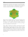

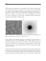


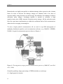


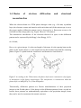
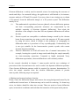


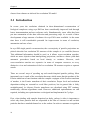


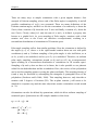

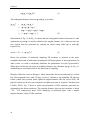
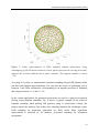


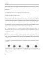
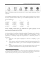


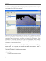


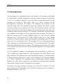
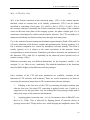
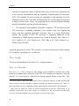
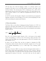
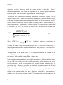
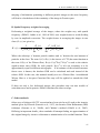

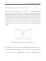
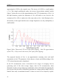
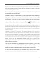
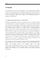

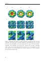
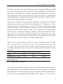

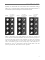
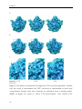
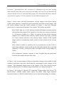
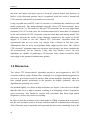
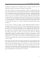


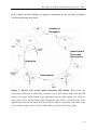

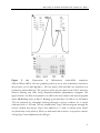

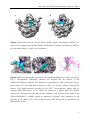

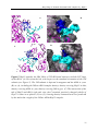
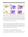

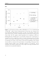
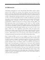


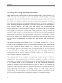


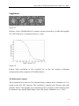


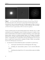
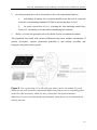
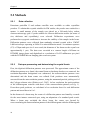

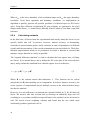

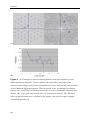

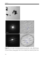

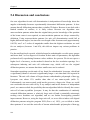


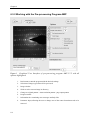
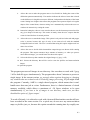


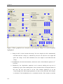


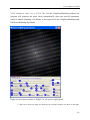
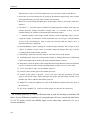


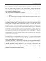


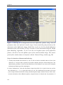


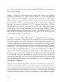


![arXiv:1208.4248v1 [math.AG] 21 Aug 2012](http://vs1.manualzilla.com/store/data/005698705_1-6d8998565962ce68b5a1333eba9cebce-150x150.png)