Download aXe User Manual version 1.42

aXe User Manual version 1.42
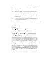
M. Kümmel
and
J. Walsh, S. Larsen, N. Pirzkal, R. Hook
23 June 2005
2
Contents
1 Description
1.1 What is aXe? . . . . . . . . . . . . . .
1.2 Slitless Spectroscopy . . . . . . . . . .
1.3 Apertures and Beams . . . . . . . . .
1.4 Pixel Extraction Tables (PET) . . . .
1.5 Generating 1D spectra . . . . . . . . .
1.6 Sky Background . . . . . . . . . . . .
1.6.1 Global Background Subtraction
1.6.2 Local Background Subtraction
1.7 Drizzling of PETs . . . . . . . . . . .
1.8 aXe Visualization . . . . . . . . . . . .
1.9 Acknowledgement . . . . . . . . . . . .
.
.
.
.
.
.
.
.
.
.
.
.
.
.
.
.
.
.
.
.
.
.
.
.
.
.
.
.
.
.
.
.
.
.
.
.
.
.
.
.
.
.
.
.
.
.
.
.
.
.
.
.
.
.
.
.
.
.
.
.
.
.
.
.
.
.
.
.
.
.
.
.
.
.
.
.
.
.
.
.
.
.
.
.
.
.
.
.
.
.
.
.
.
.
.
.
.
.
.
.
.
.
.
.
.
.
.
.
.
.
.
.
.
.
.
.
.
.
.
.
.
.
.
.
.
.
.
.
.
.
.
.
.
.
.
.
.
.
.
.
.
.
.
7
7
8
9
10
11
12
13
14
14
16
17
2 Installing aXe
2.1 Requirements . . . . . . . . . . . . . . . . .
2.1.1 aXe Distribution . . . . . . . . . . .
2.2 Installing from the aXe source distribution .
2.3 Installing from the aXe binary distributions
2.4 Validating the aXe installation . . . . . . .
2.5 aXe Mailing List . . . . . . . . . . . . . . .
2.6 aXe Support . . . . . . . . . . . . . . . . .
.
.
.
.
.
.
.
.
.
.
.
.
.
.
.
.
.
.
.
.
.
.
.
.
.
.
.
.
.
.
.
.
.
.
.
.
.
.
.
.
.
.
.
.
.
.
.
.
.
.
.
.
.
.
.
.
.
.
.
.
.
.
.
.
.
.
.
.
.
.
.
.
.
.
.
.
.
.
.
.
.
.
.
.
19
19
19
20
21
22
22
23
3 Using aXe
3.1 aXe-1.4 . . . . . . . . . . . . .
3.1.1 Python/PyRAF . . . .
3.1.2 High Level Tasks . . . .
3.1.3 aXedrizzle . . . . . . . .
3.1.4 Background Subtraction
3.1.5 aXegps . . . . . . . . .
3.2 Preparing the aXe Reduction .
3.2.1 Reduction Strategy . . .
3.2.2 MultiDrizzle . . . . . .
3.2.3 Input Object List . . . .
3.2.4 Input Image List . . . .
.
.
.
.
.
.
.
.
.
.
.
.
.
.
.
.
.
.
.
.
.
.
.
.
.
.
.
.
.
.
.
.
.
.
.
.
.
.
.
.
.
.
.
.
.
.
.
.
.
.
.
.
.
.
.
.
.
.
.
.
.
.
.
.
.
.
.
.
.
.
.
.
.
.
.
.
.
.
.
.
.
.
.
.
.
.
.
.
.
.
.
.
.
.
.
.
.
.
.
.
.
.
.
.
.
.
.
.
.
.
.
.
.
.
.
.
.
.
.
.
.
.
.
.
.
.
.
.
.
.
.
.
25
25
25
26
26
27
27
28
28
28
29
30
3
.
.
.
.
.
.
.
.
.
.
.
.
.
.
.
.
.
.
.
.
.
.
.
.
.
.
.
.
.
.
.
.
.
.
.
.
.
.
.
.
.
.
.
.
.
.
.
.
.
.
.
.
.
.
.
.
.
.
.
.
.
.
.
.
.
.
.
.
.
.
.
.
.
.
.
.
.
.
.
.
.
.
.
.
.
.
.
.
.
.
.
.
.
.
.
.
.
.
.
4
CONTENTS
3.3
3.4
Executing the High Level Tasks . . . . . . . . . . .
3.3.1 The Input Image List . . . . . . . . . . . .
3.3.2 The Input Object Lists . . . . . . . . . . .
3.3.3 The aXe Configuration Files . . . . . . . .
3.3.4 aXedrizzle and Global Sky Subtraction . . .
3.3.5 No aXedrizzle and Global Sky Subtraction
3.3.6 aXedrizzle and Background PET . . . . . .
3.3.7 No aXedrizzle and Background PET . . . .
Computing Time Requirements . . . . . . . . . . .
4 aXe tasks
4.1 AXEPREP . . . .
4.1.1 Usage . . .
4.1.2 Parameters
4.2 AXECORE . . . .
4.2.1 Usage . . .
4.2.2 Parameters
4.2.3 Output . .
4.3 DRZPREP . . . .
4.3.1 Usage . . .
4.3.2 Parameters
4.3.3 Output . .
4.4 AXEDRIZZLE . .
4.4.1 Usage . . .
4.4.2 Parameters
4.4.3 Output . .
4.5 SEX2GOL . . . . .
4.5.1 Usage . . .
4.5.2 Parameters
4.5.3 Output . .
4.6 GOL2AF . . . . .
4.6.1 Usage . . .
4.6.2 Parameters
4.6.3 Output . .
4.7 BACKEST . . . .
4.7.1 Usage . . .
4.7.2 Parameters
4.7.3 Output . .
4.8 AF2PET . . . . .
4.8.1 Usage . . .
4.8.2 Parameters
4.8.3 Output . .
4.9 PETCONT . . . .
4.9.1 Usage . . .
4.9.2 Parameters
4.9.3 Output . .
.
.
.
.
.
.
.
.
.
.
.
.
.
.
.
.
.
.
.
.
.
.
.
.
.
.
.
.
.
.
.
.
.
.
.
.
.
.
.
.
.
.
.
.
.
.
.
.
.
.
.
.
.
.
.
.
.
.
.
.
.
.
.
.
.
.
.
.
.
.
.
.
.
.
.
.
.
.
.
.
.
.
.
.
.
.
.
.
.
.
.
.
.
.
.
.
.
.
.
.
.
.
.
.
.
.
.
.
.
.
.
.
.
.
.
.
.
.
.
.
.
.
.
.
.
.
.
.
.
.
.
.
.
.
.
.
.
.
.
.
.
.
.
.
.
.
.
.
.
.
.
.
.
.
.
.
.
.
.
.
.
.
.
.
.
.
.
.
.
.
.
.
.
.
.
.
.
.
.
.
.
.
.
.
.
.
.
.
.
.
.
.
.
.
.
.
.
.
.
.
.
.
.
.
.
.
.
.
.
.
.
.
.
.
.
.
.
.
.
.
.
.
.
.
.
.
.
.
.
.
.
.
.
.
.
.
.
.
.
.
.
.
.
.
.
.
.
.
.
.
.
.
.
.
.
.
.
.
.
.
.
.
.
.
.
.
.
.
.
.
.
.
.
.
.
.
.
.
.
.
.
.
.
.
.
.
.
.
.
.
.
.
.
.
.
.
.
.
.
.
.
.
.
.
.
.
.
.
.
.
.
.
.
.
.
.
.
.
.
.
.
.
.
.
.
.
.
.
.
.
.
.
.
.
.
.
.
.
.
.
.
.
.
.
.
.
.
.
.
.
.
.
.
.
.
.
.
.
.
.
.
.
.
.
.
.
.
.
.
.
.
.
.
.
.
.
.
.
.
.
.
.
.
.
.
.
.
.
.
.
.
.
.
.
.
.
.
.
.
.
.
.
.
.
.
.
.
.
.
.
.
.
.
.
.
.
.
.
.
.
.
.
.
.
.
.
.
.
.
.
.
.
.
.
.
.
.
.
.
.
.
.
.
.
.
.
.
.
.
.
.
.
.
.
.
.
.
.
.
.
.
.
.
.
.
.
.
.
.
.
.
.
.
.
.
.
.
.
.
.
.
.
.
.
.
.
.
.
.
.
.
.
.
.
.
.
.
.
.
.
.
.
.
.
.
.
.
.
.
.
.
.
.
.
.
.
.
.
.
.
.
.
.
.
.
.
.
.
.
.
.
.
.
.
.
.
.
.
.
.
.
.
.
.
.
.
.
.
.
.
.
.
.
.
.
.
.
.
.
.
.
.
.
.
.
.
.
.
.
.
.
.
.
.
.
.
.
.
.
.
.
.
.
.
.
.
.
.
.
.
.
.
.
.
.
.
.
.
.
.
.
.
.
.
.
.
.
.
.
.
.
.
.
.
.
.
.
.
.
.
.
.
.
.
.
.
.
.
.
.
.
.
.
.
.
.
.
.
.
.
.
.
.
.
.
.
.
.
.
.
.
.
.
.
.
.
.
.
.
.
.
.
.
.
.
.
.
.
.
.
.
.
.
.
.
.
.
.
.
.
.
.
.
.
.
.
.
.
.
.
.
.
.
.
.
.
.
.
.
.
.
.
30
31
31
32
35
36
37
38
39
.
.
.
.
.
.
.
.
.
.
.
.
.
.
.
.
.
.
.
.
.
.
.
.
.
.
.
.
.
.
.
.
.
.
.
.
.
.
.
.
.
.
.
.
.
.
.
.
.
.
.
.
.
.
.
.
.
.
.
.
.
.
.
.
.
.
.
.
.
.
.
.
.
.
.
.
.
.
.
.
.
.
.
.
.
.
.
.
.
.
.
.
.
.
.
.
.
.
.
.
.
.
.
.
.
.
.
.
.
.
.
.
.
.
.
.
.
.
.
.
.
.
.
.
.
.
.
.
.
.
.
.
.
.
.
.
.
.
.
.
.
.
.
.
.
.
.
.
.
.
.
.
.
.
.
.
.
.
.
.
.
.
.
.
.
.
.
.
.
.
.
.
.
.
.
.
.
.
.
.
.
.
.
.
.
.
.
.
.
.
.
.
.
.
.
.
.
.
.
.
.
.
.
.
.
.
.
.
.
.
.
.
.
.
.
.
.
.
.
.
.
.
.
.
.
.
.
.
.
.
.
.
.
.
.
.
.
.
.
.
.
.
.
.
.
.
.
.
.
.
.
.
.
.
.
.
.
.
.
.
.
.
.
.
.
.
.
.
.
.
.
.
.
.
.
.
.
.
.
.
41
41
42
42
43
43
43
44
45
45
46
46
46
47
47
48
48
49
49
49
49
50
50
51
51
52
52
52
52
52
53
53
53
53
53
54
CONTENTS
4.10 PETFF . . . . . .
4.10.1 Usage . . .
4.10.2 Parameters
4.10.3 Output . .
4.11 PET2SPC . . . . .
4.11.1 Usage . . .
4.11.2 Parameters
4.11.3 Output . .
4.12 STAMP . . . . . .
4.12.1 Usage . . .
4.12.2 Parameters
4.12.3 Output . .
4.13 DRZ2PET . . . . .
4.13.1 Usage . . .
4.13.2 Parameters
4.13.3 Output . .
4.14 AXEGPS . . . . .
4.14.1 Usage . . .
4.14.2 Parameters
4.14.3 Output . .
5
.
.
.
.
.
.
.
.
.
.
.
.
.
.
.
.
.
.
.
.
.
.
.
.
.
.
.
.
.
.
.
.
.
.
.
.
.
.
.
.
.
.
.
.
.
.
.
.
.
.
.
.
.
.
.
.
.
.
.
.
.
.
.
.
.
.
.
.
.
.
.
.
.
.
.
.
.
.
.
.
.
.
.
.
.
.
.
.
.
.
.
.
.
.
.
.
.
.
.
.
.
.
.
.
.
.
.
.
.
.
.
.
.
.
.
.
.
.
.
.
.
.
.
.
.
.
.
.
.
.
.
.
.
.
.
.
.
.
.
.
.
.
.
.
.
.
.
.
.
.
.
.
.
.
.
.
.
.
.
.
.
.
.
.
.
.
.
.
.
.
.
.
.
.
.
.
.
.
.
.
.
.
.
.
.
.
.
.
.
.
.
.
.
.
.
.
.
.
.
.
.
.
.
.
.
.
.
.
.
.
.
.
.
.
.
.
.
.
.
.
.
.
.
.
.
.
.
.
.
.
.
.
.
.
.
.
.
.
.
.
5 Configuration of aXe tasks
5.1 Environment Variables . . . . . . . . . .
5.2 Configuration Files . . . . . . . . . . . .
5.2.1 Main Configuration File . . . . .
5.2.2 Example of a Main Configuration
.
.
.
.
.
.
.
.
.
.
.
.
.
.
.
.
.
.
.
.
.
.
.
.
.
.
.
.
.
.
.
.
.
.
.
.
.
.
.
.
.
.
.
.
.
.
.
.
.
.
.
.
.
.
.
.
.
.
.
.
.
.
.
.
.
.
.
.
.
.
.
.
.
.
.
.
.
.
.
.
.
.
.
.
.
.
.
.
.
.
.
.
.
.
.
.
.
.
.
.
.
.
.
.
.
.
.
.
.
.
.
.
.
.
.
.
.
.
.
.
.
.
.
.
.
.
.
.
.
.
.
.
.
.
.
.
.
.
.
.
.
.
.
.
.
.
.
.
.
.
.
.
.
.
.
.
.
.
.
.
.
.
.
.
.
.
.
.
.
.
.
.
.
.
.
.
.
.
.
.
.
.
.
.
.
.
.
.
.
.
.
.
.
.
.
.
.
.
.
.
.
.
.
.
.
.
.
.
.
.
.
.
.
.
.
.
.
.
.
.
.
.
.
.
.
.
.
.
.
.
.
.
.
.
.
.
.
.
.
.
.
.
.
.
.
.
.
.
.
.
.
.
.
.
.
.
.
.
.
.
.
.
.
.
.
.
.
.
.
.
.
.
.
.
.
.
.
.
.
.
54
55
55
55
55
55
56
56
56
57
57
57
57
58
58
58
58
59
59
59
. . .
. . .
. . .
file .
.
.
.
.
.
.
.
.
.
.
.
.
.
.
.
.
.
.
.
.
.
.
.
.
.
.
.
.
.
.
.
.
.
.
.
.
.
.
.
.
.
.
.
.
61
61
62
62
68
6 aXe Calibration Files
69
6.1 Sensitivity Curve . . . . . . . . . . . . . . . . . . . . . . . . . . . 69
6.2 Flat field . . . . . . . . . . . . . . . . . . . . . . . . . . . . . . . 69
7 File
7.1
7.2
7.3
7.4
7.5
7.6
7.7
7.8
7.9
7.10
7.11
7.12
Formats
Input Images . . . . . . . . .
Input Image List . . . . . . .
Input Object List . . . . . . .
Grism Object List . . . . . .
Aperture File . . . . . . . . .
Background Estimate File . .
Pixel Extraction Table . . . .
The Drizzle Prepare File . . .
The 2D Drizzled Grism Image
Extracted Spectra File . . . .
Stamp Image File . . . . . . .
Contamination File . . . . . .
.
.
.
.
.
.
.
.
.
.
.
.
.
.
.
.
.
.
.
.
.
.
.
.
.
.
.
.
.
.
.
.
.
.
.
.
.
.
.
.
.
.
.
.
.
.
.
.
.
.
.
.
.
.
.
.
.
.
.
.
.
.
.
.
.
.
.
.
.
.
.
.
.
.
.
.
.
.
.
.
.
.
.
.
.
.
.
.
.
.
.
.
.
.
.
.
.
.
.
.
.
.
.
.
.
.
.
.
.
.
.
.
.
.
.
.
.
.
.
.
.
.
.
.
.
.
.
.
.
.
.
.
.
.
.
.
.
.
.
.
.
.
.
.
.
.
.
.
.
.
.
.
.
.
.
.
.
.
.
.
.
.
.
.
.
.
.
.
.
.
.
.
.
.
.
.
.
.
.
.
.
.
.
.
.
.
.
.
.
.
.
.
.
.
.
.
.
.
.
.
.
.
.
.
.
.
.
.
.
.
.
.
.
.
.
.
.
.
.
.
.
.
.
.
.
.
.
.
.
.
.
.
.
.
.
.
.
.
.
.
71
71
73
73
75
75
77
77
78
79
80
81
81
6
CONTENTS
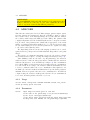
Chapter 1
Description
1.1
What is aXe?
The aXe software was designed to extract spectra in a consistent manner from all
the slitless spectroscopy modes provided by the Advanced Camera for Surveys
(ACS) which was installed on the Hubble Space Telescope in February 2002.
What we refer to as aXe is in fact a PyRAF/IRAF package with several tasks
which can be successively used to produce extracted spectra. There exist two
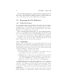
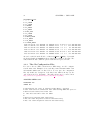
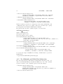
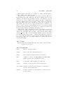
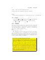
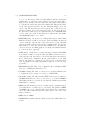
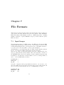
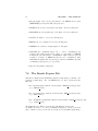
classes of aXe tasks (see Figure 1.1):
1. the Low Level Tasks work on individual grism images. All in- and output
refers to a particular grism image.
2. the High Level Tasks work on data sets. Their aim is to do certain processing steps for a set of images.
Often the High Level Tasks use the Low Level Tasks to perform a certain reduction step on each frame (see Figure 1.1).
The High Level Tasks were designed to cover all steps of the aXe reduction
without any restriction in functionality. Working with aXe therefore means to
apply the four High Level Tasks to a set of data. All tasks are controlled through
a set of configuration files which can be edited by the user and optimized for a
given data set.
The core of the software package is written using ANSI C and Python
(http://www.python.org) and is highly portable from one platform to another.
aXe uses the third party libraries CFITSIO, GSL, and WCSLIB which have
been used successfully under Linux, Solaris, and MacOS X.
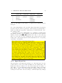
aXe is distributed as part of the STSDAS software package. Within STSDAS, aXe is located under the subpackages ’hst calib/acs/axe/’. As a relatively
young software project which is still under active development, the changes and
improvements introduced with new releases are quite large. To give users the
possibility to work always with the newest release we also distribute aXe on
7
8
CHAPTER 1. DESCRIPTION
Figure 1.1: The list of aXe tasks. The arrows indicates the interaction between
the High Level and the Low Level Tasks
the aXe webpages at http://www.stecf.org/software/aXe/index.html. On this
webpage we always offer the latest aXe release for download.
1.2
Slitless Spectroscopy
In conventional spectroscopy, slits or masks are used to allow only the light
from a small portion of the focal plane of the telescope to enter the dispersing
device (e.g. grism, grating or prism). This results in an unambiguous conversion
between pixel coordinates on the detector and wavelength.
In slitless spectroscopy there is no unique correspondence between pixel coordinates and wavelength. Consequently, the spectral reduction on the basis of
the spectroscopic data alone is impossible. Additional information concerning
the positions of the object must be added to facilitate the spectral reduction.
In aXe this is done by providing Input Object Lists at the beginning of the
reduction process. In the Input Object List the object positions are given in
the image-coordinate system or the world coordinate system. This allows the
determination of the so called reference pixel for every object. The reference
pixel is the undispersed object position in image coordinates on the grism data.
For each individual object, it is then possible to assign a wavelength to each
pixel.
In conventional spectroscopy the extraction of the 1D spectra from the 2D
data is done along the direction of the slit or mask. In slitless spectroscopy,
such a predefined extraction direction does not exist. It is in fact possible to
define a different extraction direction for each object individually by adjusting
1.3. APERTURES AND BEAMS
9
0 (B)
1 (A)
0 (B)
2 (C)
1 (A)
2 (C)
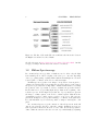
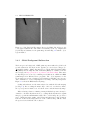
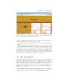
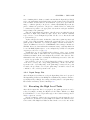
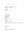
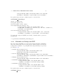
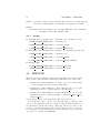
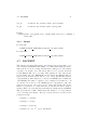
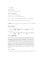
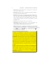
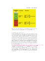
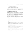
Figure 1.2: A grism image of the HUDF HRC Parallels Program (left panel)
and the aXe-beams therein (right panel). The numbers and characters give the
spectral order and the beam label in aXe. The bright areas mark the overlap of
several beams.
the wavelength assignment to be constant along the chosen extraction direction
(see Fig. 1.3). In aXe the default action is to set the extraction direction to be
parallel to the object position angle as given in the Input Object List.
The absence of slits and masks also dramatically enhances the probability
that spectra of different sources overlap each other. Even at large distances along
the dispersion direction the different orders of two objects still can overlap and
create confusion problems. aXe can mark and extract several dispersion orders
per object to properly record the source confusion or contamination for every
order of each object.
1.3
Apertures and Beams
The extraction process in aXe is done on the basis of so called BEAMs. Each
beam comprises one dispersion order of one object. The collection of all beams
(dispersion orders) of one object is called the APERTURE. The aperture is
characterized by the aperture number, which is identical to the object number
in the Input Object List. The beams are named with a single character. The
alphabetical sequence (A, B, C, ...) follows the sequence of beams defined
in the Configuration File. Each beam is defined by the coordinates of the
quadrangle which contains the pixels that are extracted together to form the
spectrum of one dispersion order of an object.
The beams follow the spectral trace of the spectrum, which is defined in
the Configuration File. While the length of a beam is set by the length of the
corresponding dispersion order, its width is adapted to the extraction width set
10
CHAPTER 1. DESCRIPTION
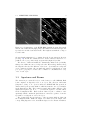
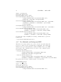
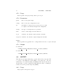
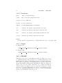
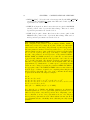
Figure 1.3: The beam geometry in a beam. A single wavelength is assigned to
each of the pixels within a beam. An extraction along an arbitrary direction
α with respect to the pixel grid is allowed. This optimizes the resolution of
the final extracted spectrum. In this figure we show α is the orientation of an
extended object.
by the user.
The left panel in Figure 1.2 shows an HRC grism exposure reduced in the
HUDF HRC Parallels Program (cleaned from cosmic-ray hits). In the right
panel, some of the beams marked and extracted in aXe are indicated. The
numbers give the spectral order, and the letters denote their corresponding
character for the configuration file used. The bright areas mark regions where
beams overlap and contaminate their spectra mutually. The different extraction
angles for the objects result in different shapes of the marked regions. For each
beam the description of the spectral trace and the wavelength description is set
up and the spectral reduction is done independently.
1.4
Pixel Extraction Tables (PET)
An important step in the aXe reduction process is the generation of the so called
Pixel Extraction Table (PET). A PET is a multi-extension fits-table which stores
in each extension the complete spectral description of all pixels of one beam.
Figure 1.3 illustrates the geometry in a beam and shows various quantities stored
in the PET. Important pixel information stored in the PET is:
• the section point, defined as the point where the spectral trace intersects
a line drawn through the center of the pixel along the extraction direction
• the distance to the section point dij
1.5. GENERATING 1D SPECTRA
11
• the trace distance Xi,j of the pixel (which is equal to the trace distance
of the section point)
• the wavelength attributed to the pixel (derived by inserting the trace distance into the dispersion function stored in the configuration file)
The PETs are read and manipulated by many aXe tasks. For example, a
flat-field correction is applied on the pixel values stored in the PETs. Since flatfielding is a wavelength dependent operation, the assignment of a wavelength
to each pixel is required before the correction values derived from a 3D flatfield
cube (see 6.2) are applied.
Also the contamination for each pixel is determined and stored in the PET.
This is done by storing for every pixel the so called contamination value, which
is the number of beams in which the pixels appears. This value is ’1’ for a
non-contaminated pixel. For the pixel in the small, white areas on Fig. 1.2
this value is ’2’, since only two beams overlap there. In crowded or deep fields
larger contamination values are also possible, of course. During the generation
of 1D spectra those contamination values are processed exactly as the pixel
values. Therefore aXe assigns to each spectral point in the final 1D spectra
an associated contamination value which marks the number of contaminations
included in the spectral point.
1.5
Generating 1D spectra
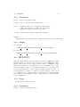
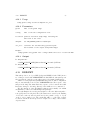
The geometry required to convert the contents of the PET to a set of one
dimensional spectra stored in the Extracted Spectra File (SPC) (see Chapt.
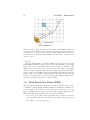
7.10) is shown in Figure 1.4. The method accounts for the geometrical rotation
of the square pixel with respect to the spectral trace and appropriately projects
each pixel onto the trace. To do this we use a weighting function which is the
fractional area of the pixel which, when projected onto the trace, falls within
the bin points 1 and 2 . The flux contained in each BEAM pixel is weighted
by this weighting function as it is projected onto separate bins (0 to 1 , 1 to
2 , and 2 to 3 in Figure 1.4) along the spectral trace. The weight is computed
by integrating over the length of the segments such as l() shown in Figure 1.4.
The length of these segments is nonzero from x0 to x3 , reaches a maximum
value of 1/sin(α), and rises and decreases linearly such that it can be described
by:

m(x − x0 ) if x0 ≤ x ≤ x1



lmax
if x1 ≤ x ≤ x2
l(x) =
m(x
−
x)
if x2 ≤ x ≤ x3

3


0
otherwise
where m = lmax /(x1 − x0 )
Integration over this function l(x) to compute w(0 , 1 ), w(1 , 2 ), and w(2 , 3 )
is trivial once one has computed x0 , ..., x3 , which may be derived from simple
trigonometry.
12
CHAPTER 1. DESCRIPTION
Figure 1.4: How a one-dimensional spectrum is created using information from
the Pixel Extraction Table (see Chapt. 7.7). Each pixel in the table is projected
onto the trace into separate wavelength bins. The number count of each pixel
is weighted by the fractional area of that pixel which falls onto a particular bin.
Once the one dimensional spectra have been generated, the final step of
flux calibrating can be performed by applying a known sensitivity curve for the
observing mode which was used. The output product of the aXe extraction
process is a FITS binary table containing the set of extracted and calibrated
spectra (Extracted Spectra File, see Chapt. 7.10).
1.6
Sky Background
aXe has two different strategies for removal of the sky background from the
spectra.
The first strategy is to perform a global subtraction of a scaled “master-sky”
frame from each input spectrum image at the beginning of the reduction process.
This removes the background signature from the images, so that the remaining
signal can be assumed to originate from the sources only and is extracted without
further background correction in the aXe reduction.
The second strategy is to make a local estimate of the sky background for
each BEAM by interpolating between the adjacent pixels on either side of the
BEAM. In this case, an individual sky estimate is made for every BEAM in
each science image.
1.6. SKY BACKGROUND
13
a
b
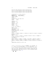
Figure 1.5: Left Panel (a):The master sky for the HRC. The holder for the
coronograph results in the ’arm’ with low sensitivity at the top. Right Panel
(b): Background estimate for the grism image shown in Fig. 1.2 with the object
regions masked.
1.6.1
Global Background Subtraction
The homogeneous background of HST grism exposures makes the global background subtraction directly from the pipeline processed science images (i.e.
flt.fits files) feasible. Master sky images for both the ACS Wide Field Channel (WFC) and the High Resolution Channel (HRC) are available from the
aXe webpages at http://www.stecf.org/software/aXe/inndex.html. These master sky images were created by combining several hundreds of WFC and HRC
grism images from different science programs. The object signatures on the
science images were removed using several techniques, including a two step median combination, to derive a high signal-to-noise image of the sky background.
Figure 1.5a shows the HRC master sky image.
Scaling and subtraction of the master sky is done with the aXe task axeprep
(see Fig. 1.1). Before scaling the master sky to the level of each science frame,
the object spectra are masked out on both the science and the master sky image.
When reducing a dataset consisting of many individual exposures, it may be
desirable to check the sky subtraction by co-adding all the sky-subtracted grism
images (e.g. with the MultiDrizzle task). The co-added image also provides a
way to quickly assess the quality of the background subtraction. Any deviations
from zero in the mean background level of the combined image will also affect
the spectra derived with the aXe reduction.
14
CHAPTER 1. DESCRIPTION
1.6.2
Local Background Subtraction
The second option for handling the sky background is to make a local estimate
of the background for each object. In this case, aXe creates an individual
background image for each object on the spectrum image. On the background
image the pixel values at the positions of the object beams are derived by
interpolating in each column between the pixel values on both sides of the
beam. The number of pixels used in the interpolation as well as the degree of
the interpolating polynomial can be chosen by the user. Figure 1.5b shows the
background image for the grism image displayed in Fig. 1.2.
The background images are then processed in much the same way as the
science images, resulting in a Background Pixel Extraction Table (BPET) for all
BEAMs in a grism image. Thus, every PET has its corresponding BPET, derived from the background image, with the spectral information of the identical
objects and beams in it. Finally, the BPET is subtracted from the PET and
the background subtracted spectra are extracted.
1.7
Drizzling of PETs
The aXe reduction scheme described up to now produces one spectrum for
each individual beam in each science image. However, datasets, such as those
obtained with ACS, often consist of several images with small position shifts
(dithers) between them. The direct approach of co-adding the 1D spectra extracted from each image to form a combined, deep spectrum has several disadvantages:
• The data is (non-linearly) rebinned twice, once when extracting the spectrum from the image and again when combining the individual 1D spectra
• A complex weighting scheme is required to flag cosmic ray affected and
bad pixels
• Low level information on the cross dispersion profile is lost when many
1D extracted spectra are combined to a deep spectrum
To circumvent these drawbacks, a new reduction scheme is available in aXe
1.4, whereby all the individual 2D spectra of an object are coadded to a single
deep 2D spectrum. The final, deep 1D spectrum is then extracted from this
combined 2D spectral image. The combination of the individual 2D spectra is
done with the “Drizzle” software, (Fruchter, A. S. & Hook, R. N. , 2002, PASP,
114, p. 144). which is available in the STSDAS package within IRAF.
The advantages of this technique as applied to slitless spectra can be summarised as follows:
• Regridding to a uniform wavelength scale and a cross-dispersion direction
orthogonal to the dispersion direction is achieved in a single step.
1.7. DRIZZLING OF PETS
15
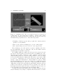
Figure 1.6: Drizzling in aXe: The object marked in panel a is extracted as
a stamp image (b). The stamp image is drizzled to an image with constant
dispersion and constant pixel scale in cross dispersion direction (c). The deep
2D drizzled image (d) is then used to extract the 1D spectrum.
• Weighting of different exposure times per pixel and cosmic-ray affected
pixels are correctly handled
• There is only one linear rebinning step to produce a 2D spectrum
• The combined 2D spectra can be viewed to detect any problems
These advantages come at the expense of a greater complexity of the reduction and significantly longer processing time. Also, the aXe drizzle reduction
currently supports only first-order spectra.
The drizzling within aXe is fully embedded in the aXe reduction flow and
uses data products and tasks created and used in the non-drizzling part of aXe.
The input for the drizzle combination consists of flatfielded and wavelength
calibrated PETs extracted for each science image, which are converted to Drizzle
PrePare files (DPP) using the drzprep task. Every first order beam in a PET
is converted to a stamp image stored as an extension in a DPP. The drzprep
task also computes the transformation coefficients which are required to drizzle
the single stamp images of each object onto a single deep, combined 2D spectral
image. These transformation coefficients are computed such that the combined
drizzle image resembles an ideal long slit spectrum with the dispersion direction
parallel to the x-axis and cross-dispersion direction parallel to the y-axis. The
wavelength scale and the pixel scale in the cross-dispersion direction can be set
by the user with keyword settings in the aXe Configuration File.
To finally extract the 1D spectrum from the deep 2D spectral image aXe uses
an (automatically created) adapted configuration file that takes into account the
16
CHAPTER 1. DESCRIPTION
Figure 1.7: Part of a webpage created by aXe2web. The coadded 2D spectrum
of the object shown here is displayed in Fig. 1.6d.
modified spectrum of the drizzled images (i.e. orthogonal wavelength and crossdispersion and the Å/pixel and arcsec/pixel scales).
A detailed discussion of the drizzling used in aXe is given in ST-ECF Newsletter, 36, p. 10.
Figure 1.6 illustrates the aXedrizzle process for one object. Panel a shows
one individual grism image with an object marked. Panel b displays the stamp
image for this object out of the grism image a. Panel c shows the drizzled grism
stamp image derived from a, and the final coadded 2D spectrum for this object
is given in panel d. Panel d shows an image combined from 112 PETs with a
total exposure time of 124 ksec. In both panels b and c the ‘holes’ resulting
from the discarded cosmic ray-flagged pixels are clearly visible.
1.8
aXe Visualization
A deep ACS WFC grism image can contain detectable spectra of hundreds to
thousands of objects, and visual checking of each spectrum is very tedious. A
quick look facility is highly desirable in order to find interesting objects (e.g.
high redshift galaxies, SN, etc) which can be highlighted for further study or
interactive spectrum extraction. For this reason we developed aXe2web, a tool
which produces browsable web pages for fast and discerning examination of
many hundreds of spectra.
Since aXe2web requires specific python modules it cannot be included in the
STSDAS software package. It is therefore distributed via the aXe webpage at
http://www.stecf.org/software/aXe/index.html in the aXe2html package.
1.9. ACKNOWLEDGEMENT
17
aXe2web uses a standard aXe input catalogue and the aXe output files to produce an html summary containing a variety of information for each spectrum.
This includes a reference number, magnitude in the magnitude system of the
direct object, the X and Y position of the direct object, its Right Ascension and
Declination, a cut-out image showing the direct object, the spectrum stamp
image showing the 2D spectrum, a 1D extracted spectrum in counts and the
same in flux units.
The user can set various keywords to influence the html output. For example,
it is possible to sort the objects with respect to an object property such as
magnitude or Right Ascension.
In order to facilitate the navigation within a data set, an overview and an
index page accompany the object pages. The overview page contains for each
object the basic information sequence number, reference number, X,Y,RA,Dec
and magnitude. The index page includes a table with the ordered reference
number of all objects. Direct links from both the overview page and the index
page guide to the corresponding locations of the objects in the object pages.
Figure 1.7 is a screenshot taken from Epoch 1 data of the HUDF HRC Parallels survey and shows the line covering the object whose coadded 2D spectrum
is shown in Fig. 1.6d. The webpages created by aXe2web are located at the
preview webpages: http://www.stecf.org/UDF/epoch1/hrc udf.html.
1.9
Acknowledgement
If the aXe software was helpful for your research work, the following acknowledgement would be appreciated:
This research has made use of the aXe extraction software, produced by ST-ECF, Garching, Germany.
18
CHAPTER 1. DESCRIPTION
Chapter 2
Installing aXe
2.1
Requirements
The following are required to run aXe:
• STSDAS 3.2 (http://www.stsci.edu/resources/software hardware/stsdas)
• PyRAF 1.1.1 (http://www.stsci.edu/resources/software hardware/pyraf)
To compile the C-code you need:
• GNU CC 2.95 or later compiler
• Gnu Scientific Libraries 1.x (http://sources.redhat.com/gsl/)
• WCStools 3.x libraries (http://tdc-www.harvard.edu/software/wcstools/)
• CFITSIO 2.x libraries (http://heasarc.gsfc.nasa.gov/docs/software/fitsio/fitsio.html)
2.1.1
aXe Distribution
aXe is distributed as part of the STSDAS software package. However, as a young
software package, aXe is still under rapid development, and the current version
distributed with STSDAS 3.3 is aXe-1.40. New aXe releases incorporate significant improvements over previous versions, but the release dates can not always
be coordinated with new STSDAS releases. We therefore offer the newest aXe1.4 release for download on the aXe webpages at http://www.stecf.org/software/aXe/index.html.
After the installation, aXe-1.4 is loaded and used as the local package taxe14
within PyRAF.
The new aXe release has tasks with the same names as in previous releases,
but the implementation (e.g. parameter settings) of the tasks may have changed.
To keep the aXe tasks in your STSDAS distribution separate from the new aXe
tasks downloaded from the aXe webpages, the aXe tasks distributed via our
webpage always start with the letter t. For example, the task tsex2gol in the
19
20
CHAPTER 2. INSTALLING AXE
(local) taxe14 package corresponds to the task sex2gol in STSDAS, taf2pet
in taxe14 corresponds to af2pet in STSDAS and so on. While this manual
describes aXe-1.42 and the aXe-1.42 tasks distributed via aXe webpages with
a t as prefix, the tasks are named with the non-prefix version throughout the
manual. If you work with aXe-1.42 tasks, don’t forget to put a t in front of every
command you find in the manual. Otherwise you may still use the old aXe-1.40
or even aXe-1.3 equivalent with a different syntax and different behaviour.
2.2
Installing from the aXe source distribution
After downloading the aXe-1.4 tarball
(http://www.stecf.org/software/aXe/taxe14 download.php), move it to the installation directory /your/aXe1.4/path and unpack it there with:
>gunzip aXe1.42-taxe14src.tar.gz
>tar -xvf aXe1.42-taxe14src.tar
aXe-1.4 consists of a part written in ANSI C and a second part written in
Python (www.python.org). For the C part a configure script is included with
aXe. To configure and then compile the C tasks do the following:
>cd taxe14/ccc
>./configure
For MacsOSX, the option ”–build=powerpc” must be added to the configurecommand. If some libraries used by aXe are not installed in the usual places,
online parameters must be used to tell the configure script where to find them.
For example
./configure --with-cfitsio-prefix=/your_axelibs/cfitsio
--with-gsl-prefix=/your_axelibs/gsl-1.0
--with-wcstools-prefix=/your_axelibs/wcstools-3.0.4
specifies explicitly the location of the GSL and the CFITSIO library. Follow
the instructions given by the configure script to solve problems. The configure
script generates a Makefile which is used to compile the aXe-tasks. Type
>make
to execute the Makefile and create the tasks. The tasks must be installed in the
bin directory of the taxe14 package. Simply execute
>make install
to move the binaries to their proper location.
On the Python side there exists a similar script to compile the code. Go to
the Python directory and compile the Python code there with:
>cd ../iraf
>python compileaXe.py .
2.3. INSTALLING FROM THE AXE BINARY DISTRIBUTIONS
21
If all went well, aXe-1.42 is now ready. The new package with its tasks must
be declared in PyRAF. To do this, add the following lines near the end of your
login.cl file, or in loginuser.cl:
reset
task
reset
taxe14
taxe14.pkg
helpdb
= /your/aXe1.4/path/taxe14/iraf/
= taxe14$taxe14.cl
= (envget("helpdb") //",taxe14$lib/helpdb.mip")
The next time PyRAF is launched, the package taxe14 should be available. It
can then be loaded as any other package by simply typing its name:
--> taxe14
The taXe14 software package was developed by the ACS group
of the ST-ECF. It contains the new version 1.42 of the axe
software. Any questions regarding this software can be
directed to: [email protected]
taxe14/:
taf2pet
taxecore
taxedrizzle
taxegps
taxeprep
tbackest
tdrz2pet
tdrzprep
tgol2af
tpet2spc
tpetcont
tpetff
tsex2gol
tstamps
The message which appears during the loading of the package and the task
overview indicate that everything went OK and that the tasks can be used from
now on. The package can be used by more than one user. Other users only
have to modify their login.cl or loginuser.cl as described above to access
the aXe1.4 package and the tasks within it (provided that they have access to
the installation directory).
aXe-1.4 was successfully built and tested under Red Hat Linux 9 and Solaris
2.8. It should be no problem to install aXe-1.4 under other Unix or Unix-like
operating systems such as HPUX or MacOSX.
2.3
Installing from the aXe binary distributions
Several distributions of aXe with compiled statically linked C tasks are available
for download from the aXe web pages. Download the source tarball aXe1.42taxe14src.tar.gz, and then select and download the binary distribution which is
appropriate for your platform. After downloading the aXe source distribution,
move it to your preferred location /your/aXe1.4/path and unpack it there
with:
>gunzip aXe1.42-taxe14src.tar.gz
>tar -xvf aXe1.42-taxe14src.tar
Then move the C-binaries to their proper location and unpack them there:
22
CHAPTER 2. INSTALLING AXE
>mv aXe1.42-<arch>.bin.tar.gz taxe14/iraf/bin/.
>cd taxe14/iraf/bin/
>gunzip aXe1.42-<arch>.bin.tar.gz
>tar -xvf aXe1.42-<arch>.bin.tar
The Python code must still be compiled. To do that execute:
>cd ..
>python compileaXe.py .
aXe-1.4 is now ready. Declare the new package in PyRAF by adding the following lines near the end of your login.cl file, or in loginuser.cl:
reset
task
reset
taxe14
taxe14.pkg
helpdb
= /your/aXe1.4/path/taxe14/iraf/
= taxe14$taxe14.cl
= (envget("helpdb") //",taxe14$lib/helpdb.mip")
The next time PyRAF is launched, the package taxe14 is available. It can be
loaded with “-->taxe14” from the PyRAF shell.
2.4
Validating the aXe installation
Test data with grism and prism images can can be obtained from our web
site. Un-zip and un-tar the test data file in a clean directory and follow the
instructions given in the README file. The grism test data consist of a set of
science frames taken from the HUDF HRC Parallels program. Figs. 1.2, 1.5 and
1.6 show some of the data products generated during the test reduction.
The prism test data was taken as part of the calibration proposal 10391 (PI:
S.S. Larsen).
Reference spectra generated by running aXe-1.42 on the test data also supplied as part of the test package. If the output obtained by running aXe-1.42
on the test data is identical to these reference spectra, the proper working of
aXe-1.42 is assured.
2.5
aXe Mailing List
We have installed an aXe mailing list to keep users informed about new developments and updates concerning aXe. To the subscribers the mailing list
also offers the opportunity to share and discuss their experiences with aXe. We
encourage all aXe users to participate and use the mailing list as a discussion
forum for aXe and aXe related issues. The aXe software package is still evolving,
and the communication between the software developers and the users is very
important to improve the future versions of aXe.
The subscription to the aXe mailing list is done by sending an email to
[email protected] with the content subscribe [email protected] in the mail
body.
2.6. AXE SUPPORT
23
To unsubscribe from the aXe mailing list, please send an email to
[email protected] with the content unsubscribe [email protected] in the
mail body.
2.6
aXe Support
The ACS group at the Space Telescope - European Coordinating Facility (STECF)
is responsible for the support of the spectroscopic modes of ACS. The development of the aXe software package and the preparation of calibration products
for the reduction are key components of this support. To request further help
and information concerning aXe or the calibration products, please contact us
with an email to [email protected].
24
CHAPTER 2. INSTALLING AXE
Chapter 3
Using aXe
This chapter shows the various ways and strategies to reduce slitless spectroscopy data with aXe. The different methods to produce the final, calibrated
1D spectra are presented and discussed. We also provide example scripts showing how the various aXe tasks can be applied to reduce a given data set.
Note on aXe Input slitless FITS file formats:
In order to produce flux calibrated output, aXe should be used with input files which have been time normalized and gain corrected, i.e. in units
of electrons/second. The units of the direct image is not important since
this file is only used to perform astrometric registration between the direct and slitless images. It is nevertheless convenient to use direct images
which are in electrons/second too when generating the input source catalog
with SExtractor in order to have proper magnitudes in the Input Object
List. This allows for the same magnitude cutoffs MMAG EXTRACT and
MMAG MARK to be used in the configuration file (see Chapt. 5.2) when
using aXe with data which were taken with different integration times.
3.1
aXe-1.4
Version 1.4 of aXe differs from earlier aXe releases (1.2 or 1.3) in several ways
and users who are familiar with previous versions of aXe should be prepared
that it may take some time to familiarise themselves with the new “look and
feel” of aXe-1.4. We believe, however, that the benefits of the new features in
aXe by far outweigh the inconvenience of having to learn new tasks. In this
chapter we present and explain the new features and philosophies that come
along with aXe-1.4.
3.1.1
Python/PyRAF
Some of the aXe tasks are now written in Python, an interpreted, interactive,
object-oriented programming language (see http://www.python.org). One of
25
26
CHAPTER 3. USING AXE
the main reasons for this change was the implementation of the aXedrizzle
technique described in Chapt. 3.1.3. In Python, IRAF commands can be called
directly through their PyRAF interfaces, and it is therefore easy to use the
standard IRAF implementation of drizzle within aXedrizzle. The easy access to
the standard IRAF tasks also allowed the implementation of the task axeprep,
which extends aXe to perform some preparatory steps for which users had been
required to write their own scripts in previous versions of aXe.
aXe-1.4 is closely tied to PyRAF, the new command language for running
IRAF tasks (see http://www.stsci.edu/resources/software hardware/pyraf). The
aXe versions which are distributed independently of STSDAS (see Chapt. 2.1.1)
also include PyRAF frontends, and the normal procedure there is to install aXe
as a local PyRAF package, rather than running the aXe tasks as separate Unix
commands (as in previous aXe versions). This also makes it straight-forward to
integrate aXe tasks into IRAF/PyRAF scripts. aXe tasks no longer have to be
applied in external shell scripts, but can become an integral part of any data
reduction scheme implemented in IRAF/PyRAF.
3.1.2
High Level Tasks
Until aXe-1.3 all aXe tasks performed only a single reduction step on an individual spectrum image. The task sex2gol creates a Grism Object List for one
grism image. Then the task gol2af generates an Aperture File for that grism
image, af2pet produces a Pixel Extraction Table for that grism image, and so
on.
aXe-1.4 introduces a new class of High Level Tasks. The High Level Tasks
work on Input Image Lists, and are designed to perform a reduction step on an
entire data set. To work on the individual images the High Level Tasks often
employ the old Low Level Tasks of aXe (see Fig. 1.1).
Each High Level Task combines several reduction steps, e.g. the whole aXe1.3 reduction is now executed within the High Level Task axecore. This strategy keeps the number of tasks which the user actually has to use and understand
low. Although the capabilities of the aXe software have been greatly extended
in aXe-1.4, only four High Level Tasks are required to perform a full reduction
of a set of ACS grism images with aXe-1.4.
3.1.3
aXedrizzle
The drizzling of grism spectra is probably the most significant addition in aXe1.4. This is the first implementation of the drizzle code to combine spectral data,
but the overall methodology presented here can in principle also be applied
in other reduction packages for spectral data. While the main advantages of
aXedrizzle were discussed in Chapt. 1.7, a more elaborate discussion of various
practical issues is given below.
The use of drizzle in aXe makes the application of non-trivial weights in
the extraction of 1D spectra necessary. The masking of bad pixels or cosmic
ray affected pixels and the incomplete coverage of object beams on individual
3.1. AXE-1.4
27
grism images can result in a very inhomogeneous distribution of exposure times
(and, therefore, signal-to-noise ratio) across the 2D drizzled grism images. To
compensate for the variations in the signal-to-noise ratio, a weight is assigned
to each pixel and, during the extraction of the 1D spectra, the weights are taken
into account. Within each set of pixels that is coadded to a final, 1D spectral
element, the value assigned to an individual pixel weight is proportional to its
relative exposure time (see note on page 79). While the use of weights for now
is a necessity caused by the irregular coverage of the total field of view, this first
application opens the door for the implementation of more refined weighting
schemes such as optimal extraction in future aXe releases.
To extract the final 1D spectra from the 2D drizzled grism images, any
longslit extraction program can be used. All the necessary information for
calibration and extraction is given in the aXe configuration file and the various
other aXe files. Thus, aXe users are not restricted to using aXe tasks for the
1D extraction, but can also apply alternative extraction methods e.g. to make
use of a more advanced weighting schemes.
In a pilot study, the aXedrizzle reduction scheme was used for the reduction of
the Hubble Ultra Deep Field (HUDF) HRC Parallels data. The results can be
seen on the preview webpages at http://www.stecf.org/UDF/HRCpreview.html.
3.1.4
Background Subtraction
Another new feature introduced in aXe-1.4 is the option of using a global background subtraction, based on a scaled master sky image. Our experience with
application of this technique to the HUDF HRC Parallels data was very encouraging. Also the Grism ACS Program for Extragalactic Science (GRAPES), PI
Sangeeta Malhotra (see http://www-int.stsci.edu/ san/Grapes/, and Pirzkal et
al. 2004 for more details) have used this technique to subtract the background
prior to the aXe reduction.
Nevertheless, the stability of the grism background and the long term applicability of the master sky images remain poorly quantified. We recommend
combining the sky-subtracted grism images with the MultiDrizzle task in
STSDAS in order to verify that the master sky subtraction went well and
resulted in a mean background level close to zero (see Chapt. 1.6.1). New
master sky images as well as the latest information concerning aXe in general and also the background subtraction are posted on the aXe webpages at
http://www.stecf.org/software/aXe/index.html.
3.1.5
aXegps
A small, but eventually very useful feature of aXe-1.4 is the task axegps (see
Chapt. 4.14 for details). This task prints the spectral properties of an individual
pixel onto the screen. The spectral properties are e.g. the wavelength at pixel
center, the dispersion, the distance to the trace and the trace distance of the
section point (closest point on the trace). Of course a unique spectral solution
can only be derived with respect to a reference beam (see Chapt. 1.2).
28
CHAPTER 3. USING AXE
The task axegps assists the user to find important spectral features directly
on the unprocessed and undrizzled flt-frames. On the other hand it is also possible to trace back from strange or suspicious features on extracted 1D spectra
to the corresponding positions on the original, unprocessed images.
3.2
3.2.1
Preparing the aXe Reduction
Reduction Strategy
Before actually preparing and performing the data reduction, the user must decide which data reduction strategy to follow. The main decisions are whether
aXedrizzle is used or not and whether the background subtraction is done globally with the master background or with a local background for each beam (see
Chapt. 1.6 for a comparison of the two methods).
The recommended reduction strategy is to do a global background subtraction and to use aXedrizzle. For the typical survey type data, this is the best
way to reduce ACS grism data. In case only individual spectra in crowded fields
are to be reduced, the reduction with a background PET may have advantages.
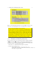
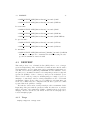
Depending on the reduction strategy, different High Level aXe Tasks have
to be applied to reduce the spectra. Table 3.1 lists the tasks and the order in
which to apply them for the various reduction strategies.
3.2.2
MultiDrizzle
After the reduction strategy has been decided, the first reduction step is to run
MultiDrizzle on the grism images. MultiDrizzle is an interface for performing all the tasks necessary for registering dithered HST images. The program
automatically performs cosmic ray rejection, removes geometric distortions and
performs the final image combination with “drizzle”.
The image combination is done for two reasons:
1. the combined image gives a good impression on the quality of the data
and the signal-to-noise level of the various object spectra
2. MultiDrizzle runs a cosmic ray detection algorithm, and the dq-extention
of the flt-images is updated with the information on all cosmic rays detected in the MultiDrizzle run. Running MultiDrizzle is therefore a
simple way to perform a cosmic ray detection on the grism images.
While MultiDrizzle can combine slitless grism images, no wavelength sensitive flatfield is applied to the images (see Chapt. 6.2). Moreover, the field
dependence of the grism spectra and the field dependent wavelength calibration are not taken into account in the combination process. It is therefore not
recommended to extract the spectra directly from the MultiDrizzle combined
grism images.
It is also possible to use other programs to identify cosmic ray hits on the grism
images. Information on cosmics should be transported into the dq-extension of
3.2. PREPARING THE AXE REDUCTION
number
1.
2.
3.
4.
5.
+aXedrizzle/
+master sky
axeprep
axecore
drzprep
axedrizzle
-aXedrizzle/
+master sky
axeprep
axecore
+aXedrizzle/
-master sky
axeprep
axecore
drzprep
axedrizzle
axedrizzle
29
-aXedrizzle/
-master sky
axeprep
axecore
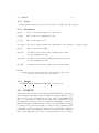
Table 3.1: The high level aXe tasks to be applied in the different reduction
strategies.
the corresponding flt-image. aXe can exclude flagged pixels in the dq-extention
from the reduction. In the dq-extention cosmic ray affected pixels should be
marked by adding the appropriate dq-flag 4096 (see ACS Data handbook) to
the original dq value.
Users with old versions of MultiDrizzle (before STSDAS 3.3) will find mask
files with the extension ” flt sci? mask.pl” (? is a placeholder for the extension
number). In those mask files good pixels have the value ’1’ and cosmic ray
affected one the value ’0’. Before starting the aXe reduction the user should
transport the cosmic ray information from the mask files into the corresponding
dq-extension of the flt-files.
Input Object Lists versus Input Image Lists
Although the names are strikingly similar, Input Object Lists and Input
Image Lists are fundamentally different. The format of an Input Object
List is identical to the SExtractor ASCII catalogue format. An Input Object List contains positions and further (SExtractor-) information for all
astronomical sources on the associated direct or grism image. The Input
Object List is used as an input in the Low Level aXe Task sex2gol to
derive a Grism Object List (GOL, see Chapt. 7.4) for a grism image.
On the other hand, Input Image Lists are an input parameter in all High
Level Tasks. An Input Image List contains on each row the name of a grism
image and additional information which is necessary to run the aXe task on
that grism image. Those additional information are the name(s) of Input
Object List(s) and, optionally, a direct image name and a dmag-value. The
exact descriptions of Input Object Lists and Input Image Lists plus their
formats are on Chapts. 7.3 and 7.2, respectively.
3.2.3
Input Object List
The preparation of the Input Object List is one of the last steps before the
actual reduction of the spectra with the High Level aXe Tasks starts. The
Input Object List (see chapter 7.3 for the exact format) can refer either to a
direct image or to the grism image itself. If the third column of the Input
Image List (see Chapt. 7.1) used in the High Level Tasks is a string, the entry
is interpreted as the name of the direct image to which the Input Object List(s)
30
CHAPTER 3. USING AXE
refer. A missing third column or a number means that the Input Object List(s)
refer to the grism image itself. In the latter case the format for the Object List
is more flexible, and the values for the individual objects can be given either in
image coordinates (pixels) or in global coordinates (RA/DEC). If present the
pixel coordinates are preferred to the global coordinates. However, with global
coordinates it is possible to use appropriate cutouts from catalogues assembled
independently of the grism data.
Since the requirements and premises of the aXe users concerning the targets
and therefore Input Object Lists are quite diverse, there exists no standard
recipe on how to create an Input Object List. We also do not offer an aXe task
to perform that job.
A quite widespread scenario is that there exist a list of grism exposures, and
a basic object catalogue which comprises all objects in the area covered by the
grism exposures. This basic object catalogue might be taken from an archive or
derived via SExtractor from a set of MultiDrizzled direct images. In this case
STSDAS offers some basic tasks such as tranback, traxy or xytosky which can
be used in IRAF/PyRaf scripts to create an Input Object Lists for each grism
exposure (see also Note on page 75).
Usually there are are several Input Object Lists to reduce a set of grism
exposures. Care must be taken that each object is assigned an identical object
identification number in the various Input Object Lists of the data set, since
this number is the only way to identify the individual spectra and to derive the
coadded, deep spectrum of an object.
It is possible to give an object in the Input Object List a position outside
of the area covered by the corresponding grism image. In the case that the
spectrum of the object falls partly on the grism image, but its reference point
is outside, the spectrum covered by the grism image can still be reduced and
contribute to the coadded spectrum of the object.
3.2.4
Input Image List
After the Input Objects Lists are ready, the Input Image List can be prepared.
The Input Image List is used in all High Level Tasks in the parameter inlist to
specify Input Object List(s), direct image and dmag-value for each grism image.
Its format is extensively described in Chapt. 7.2.
3.3
Executing the High Level Tasks
After all the input files have been prepared, the grism spectra now can be
reduced by simply executing the High Level aXe Tasks. Which set of High
Level Tasks have to be used depends strongly on the reduction strategy chosen.
Table 3.1 gives an overview.
For the remainder of this section we present the various input files for a
typical data set and list the necessary High Level Tasks for the different reduction scenarios. The High Level Tasks are listed in the correct order in both the
3.3. EXECUTING THE HIGH LEVEL TASKS
31
interactive version as well as the version used in a python script.
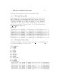
3.3.1
The Input Image List
The Input Image List aXetest.lis given in this example is for a data set consisting of WFC images. The Input Image List refers to the direct image listed
in the third column. There is one Input Object List for each of the two science
extensions in the WFC data (see Chapt. 7.1 and Fig. 7.1 for an explanation
on chip number versus extension numbers in WFC images). All files are expected to be located in the directory pointed to by the environment variable
AXE IMAGE PATH (see Chapt. 5.1).
aXetest.lis:
j8qq50nkq_flt.fits
j8qq51pmq_flt.fits
j8qq52ntq_flt.fits
j8qq10ikq_flt.fits
j8qq11juq_flt.fits
j8qq11k0q_flt.fits
j8qq12kgq_flt.fits
3.3.2
j8qq53nkq_2.cat,j8qq53nkq_1.cat
j8qq54pmq_2.cat,j8qq54pmq_1.cat
j8qq55ntq_2.cat,j8qq55ntq_1.cat
j8qq16ikq_2.cat,j8qq16ikq_1.cat
j8qq17juq_2.cat,j8qq17juq_1.cat
j8qq18k0q_2.cat,j8qq18k0q_1.cat
j8qq19kgq_2.cat,j8qq19kgq_1.cat
j8qq53nkq_flt.fits
j8qq54pmq_flt.fits
j8qq55ntq_flt.fits
j8qq16ikq_flt.fits
j8qq17juq_flt.fits
j8qq18k0q_flt.fits
j8qq19kgq_flt.fits
0.2
0.15
-0.4
0.0
0.05
-.5
0.32
The Input Object Lists
As examples, the first lines of the Object Lists j8qq53nkq 1.cat and j8qq54pmq 1.cat,
both produced by SExtractor, are listed below:
j8qq53nkq 1.cat:
#
#
#
#
#
#
#
#
#
#
#
#
1 X_IMAGE
2 Y_IMAGE
3 NUMBER
4 X_WORLD
5 Y_WORLD
6 MAG_AUTO
7 A_IMAGE
8 B_IMAGE
9 THETA_IMAGE
10 A_WORLD
11 B_WORLD
12 THETA_WORLD
4191.57 323.45 1
4266.90 378.97 5
4259.20 365.97 6
4237.82 374.40 7
3991.36 528.52 8
4304.72 435.51 9
53.1655096
53.1640349
53.1642830
53.1643802
53.1647451
53.1629142
-27.8284792
-27.8288907
-27.8289079
-27.8285958
-27.8245487
-27.8288662
22.71 13.6 13.6 -11.5 NaN NaN NaN
27.02 3.0 3.0 22.4 NaN NaN NaN
28.66 3.0 3.0
6.1 NaN NaN NaN
25.19 3.0 3.0 27.6 NaN NaN NaN
20.89 14.3 14.3 60.1 NaN NaN NaN
28.65 3.0 3.0 -4.5 NaN NaN NaN
32
CHAPTER 3. USING AXE
j8qq54pmq 1.cat:
#
#
#
#
#
#
#
#
#
#
#
#
1 X_IMAGE
2 Y_IMAGE
3 NUMBER
4 X_WORLD
5 Y_WORLD
6 MAG_AUTO
7 A_IMAGE
8 B_IMAGE
9 THETA_IMAGE
10 A_WORLD
11 B_WORLD
12 THETA_WORLD
4187.78 312.78 1
4263.11 368.29 5
4255.41 355.29 6
4234.03 363.72 7
3987.57 517.82 8
4300.93 424.82 9
53.1655096
53.1640349
53.1642830
53.1643802
53.1647451
53.1629142
-27.8284792
-27.8288907
-27.8289079
-27.8285958
-27.8245487
-27.8288662
22.71 13.6 13.6 -11.5 NaN NaN NaN
27.02 3.0 3.0 22.4 NaN NaN NaN
28.66 3.0 3.0
6.1 NaN NaN NaN
25.19 3.0 3.0 27.6 NaN NaN NaN
20.89 14.3 14.3 60.1 NaN NaN NaN
28.65 3.0 3.0 -4.5 NaN NaN NaN
As can be verified from the World coordinates (X WORLD, Y WORLD), objects with
the identical numbers (NUMBER) in the two Input Object Lists are the same. The
values NaN in the last column are placeholders and are neglected in aXe.
3.3.3
The aXe Configuration Files
For each of the two FITS extensions in a WFC image, an aXe configuration file must exist. Examples of two such files, named ACS.WFC.CHIP1.conf
and ACS.WFC.CHIP2.conf, are listed below. To save space the configuration
files only include the description of the first beam, which is in any case the
only beam treated by aXedrizzle. The full versions can be retrieved from
http://www.stecf.org/instruments/acs/calib/all Cycles/WFC/.
ACS.WFC.CHIP1.conf:
INSTRUMENT ACS
CAMERA WFC
#
#
#
#
#
#
#
#
Calibrations for Cycle 11 onward for WFC CHIP 1; released
June 2004 based on calibration data taken during SMOV and Cycle 11.
Revised (3rd order) flat field cube:
WFC.flat.cube.CH1.2.fits for CHIP1
Revised 1st and 2nd order sensitivity
New 0th order dispersion solution and sensitivity
New -1st order dispersion solution and sensitivity
3.3. EXECUTING THE HIGH LEVEL TASKS
33
# New -2nd order dispersion solution and sensitivity
# New -3rd order dispersion solution and sensitivity
SCIENCE_EXT SCI ; Science extension
DQ_EXT DQ
; DQ extension
ERRORS_EXT ERR ; Error extension
OPTKEY1 CCDCHIP
OPTVAL1 1
FFNAME WFC.flat.cube.CH1.2.fits
DQMASK
16383
DRZRESOLA 40.0
DRZSCALE
0.05
DRZLAMB0 4770.0
DRZXINI
15.0
DRZROOT
aXetest
# First order (BEAM A)
BEAMA -30 160
MMAG_EXTRACT_A 30.0
MMAG_MARK_A
30.0
# Trace description, 1st order
DYDX_ORDER_A 1
DYDX_A_0 0.0 0.0 0.0 0.0 0.0 0.0
DYDX_A_1 -0.0357549 1.05903e-6 -5.09607e-6 -9.18057e-11 6.21825e-11 9.56794e-11
# X and Y Offsets
XOFF_A 0.0
YOFF_A -0.501521 -0.000067788 -0.000178108 2.52541e-8 1.3043e-7 -3.49966e-9
# Dispersion solution, 2nd order
DISP_ORDER_A 2
DLDP_A_0 4771.61 0.0370233 -0.000189538 -0.0000103637 -1.39952e-6 3.20763e-6
DLDP_A_1 36.4556 0.00133904 -0.00113125 3.81861e-8 -8.88458e-8 1.02802e-7
DLDP_A_2 0.0101197 9.65156e-7 -4.33325e-7 -2.0178e-10 6.50773e-11 -5.05835e-10
#
SENSITIVITY_A ACS.WFC.1st.sens.5.fits
ACS.WFC.CHIP2.conf:
INSTRUMENT ACS
CAMERA WFC
#
#
#
#
#
#
Calibrations for Cycle 11 onward for WFC CHIP 2; released
June 2004 based on calibration data taken during SMOV and Cycle 11.
Revised (3rd order) flat field cube:
WFC.flat.cube.CH2.2.fits for CHIP2
Revised 1st and 2nd order sensitivity
34
#
#
#
#
CHAPTER 3. USING AXE
New
New
New
New
0th order dispersion solution and sensitivity
-1st order dispersion solution and sensitivity
-2nd order dispersion solution and sensitivity
-3rd order dispersion solution and sensitivity
SCIENCE_EXT SCI ; Science extension
DQ_EXT DQ
; DQ extension
ERRORS_EXT ERR ; Error extension
OPTKEY1 CCDCHIP
OPTVAL1 2
FFNAME WFC.flat.cube.CH2.2.fits
DQMASK
16383
DRZRESOLA 40.0
DRZSCALE
0.05
DRZLAMB0 4770.0
DRZXINI
15.0
DRZROOT
aXetest
# First order (BEAM A)
BEAMA -30 160
MMAG_EXTRACT_A 30.0
MMAG_MARK_A
30.0
# Trace description, 1st order
DYDX_ORDER_A 1
DYDX_A_0 0 0 0
DYDX_A_1 -0.0246422 9.28567e-7 -5.49754e-6 -9.18057e-11 6.21825e-11 9.56794e-11
# X and Y offsets
XOFF_A 0
YOFF_A -0.143255 -0.00034143 -0.000163423 2.52541e-8 1.3043e-7 -3.49966e-9
# Dispersion solution, 2nd order
DISP_ORDER_A 2
DLDP_A_0 4786.13 0.0399595 -0.0136488 -0.0000103637 -1.39952e-6 3.20763e-6
DLDP_A_1 39.2815 0.00152543 -0.00156261 3.81861e-8 -8.88458e-8 1.02802e-7
DLDP_A_2 0.00880236 8.28624e-7 1.68916e-6 -2.0178e-10 6.50773e-11 -5.05835e-10
#
SENSITIVITY_A ACS.WFC.1st.sens.5.fits
As can be seen from the two keywords “OPTKEY1” and “OPTVAL1”, the
two configuration files ACS.WFC.CHIP1.conf and ACS.WFC.CHIP2.conf give
the trace description and spectral description for chip 1 and 2, respectively.
The location of the configuration files (also the flatfield, sensitivity files, and
master sky images) is the directory pointed to by the environment variable
AXE CONFIG PATH (see Chapt. 5.1).
3.3. EXECUTING THE HIGH LEVEL TASKS
35
Figure 3.1: The Input Image List aXetest.lis and a High Level aXe-1.4 Task.
The arrows connect input which refers to the identical science extension.
Note on data with multiple science extensions
For grism data with several science extensions (e.g. ACS WFC images), the
input given in the second column of the Input Image List (the Input Object
Lists), as well as the parameter backims in axeprep and the parameter
configs in all High Level Tasks, must be a comma separated list. Each
item in the list gives the input for a specific extension. The same relative
positions in those lists must specify the same extensions. As Fig. 3.1 shows,
this means that e.g. the Input Object List given as the second item in the
Input Image List targets the same extension as the second item in the
parameter backims and the second item in the parameter configs.
3.3.4
aXedrizzle and Global Sky Subtraction
In this reduction scenario the background is subtracted using a mastersky
(cr 2.cmb.fits and cr 1.cmb.fits for data in science extension 2 and 1, respectively). For each object the 2D spectra on the individual grism images are
combined to a deep, 2D grism spectrum with aXedrizzle, then the 1D spectrum
is extracted from the coadded 2D grism spectrum.
The sequence of commands interactively applied in PyRAF is:
-->axeprep inlist="aXetest.lis"
configs="ACS.WFC.CHIP1.conf,ACS.WFC.CHIP2.conf"
backgr="YES" backims="cr_2.cmb.fits,cr_1.cmb.fits" mfwhm="2.0"
norm="YES" histogram="YES"
36
CHAPTER 3. USING AXE
-->axecore inlist="aXetest.lis"
configs="ACS.WFC.CHIP1.conf,ACS.WFC.CHIP2.conf" back="NO"
extrfwhm=4.0 drzfwhm=3.0 spectr="YES" rectified="YES")
-->drzprep inlist="aXetest.lis"
configs="ACS.WFC.CHIP1.conf,ACS.WFC.CHIP2.conf" back="NO")
-->axedrizzle inlist="aXetest.lis"
configs="ACS.WFC.CHIP1.conf,ACS.WFC.CHIP2.conf"
infwhm=4.0 outfwhm=3.0 back="NO" makespc="YES")
The line breaks are added here for clarity, but on the actual command line each
command should be given as one string. The most convenient way to specify
the task parameters is with the IRAF epar mechanism.
In a python script, the same command sequence looks as follows:
aXedrizzle mastersky.py:
import os,string,time
from pyraf import iraf
from iraf import axe14, stsdas
iraf.axeprep(inlist="aXetest.lis",
configs="ACS.WFC.CHIP1.conf,ACS.WFC.CHIP2.conf",
backgr="YES", backims="cr_2.cmb.fits,cr_1.cmb.fits", mfwhm="2.0",
norm="YES", histogram="YES")
iraf.axecore(inlist="aXetest.lis",
configs="ACS.WFC.CHIP1.conf,ACS.WFC.CHIP2.conf", back="NO",
extrfwhm=4.0, drzfwhm=3.0, spectr="YES", rectified="YES")
iraf.drzprep(inlist="aXetest.lis",
configs="ACS.WFC.CHIP1.conf,ACS.WFC.CHIP2.conf", back="NO")
iraf.axedrizzle(inlist="aXetest.lis",
configs="ACS.WFC.CHIP1.conf,ACS.WFC.CHIP2.conf",
infwhm=4.0, outfwhm=3.0, back="NO", makespc="YES")
To execute the script in PyRAF, the following command must be given in a
PyRAF shell:
--> pyexecute("aXedrizzle_mastersky.py")
3.3.5
No aXedrizzle and Global Sky Subtraction
Here the background is globally subtracted using master sky images. The coaddition of the individual 2D spectra with aXedrizzle is not done. The command
sequence is a subset of the command sequence in the last example:
-->axeprep inlist="aXetest.lis"
configs="ACS.WFC.CHIP1.conf,ACS.WFC.CHIP2.conf"
backgr="YES" backims="cr_2.cmb.fits,cr_1.cmb.fits" mfwhm="2.0"
norm="YES" histogram="YES"
-->axecore inlist="aXetest.lis"
3.3. EXECUTING THE HIGH LEVEL TASKS
37
configs="ACS.WFC.CHIP1.conf,ACS.WFC.CHIP2.conf" back="NO"
extrfwhm=3.0 drzfwhm=0.0 spectr="YES" rectified="YES")
In a python script, the same command sequence looks as follows:
noaXedrizzle mastersky.py:
import os,string,time
from pyraf import iraf
from iraf import axe14, stsdas
iraf.axeprep(inlist="aXetest.lis",
configs="ACS.WFC.CHIP1.conf,ACS.WFC.CHIP2.conf",
backgr="YES", backims="cr_2.cmb.fits,cr_1.cmb.fits", mfwhm="2.0",
norm="YES", histogram="YES")
iraf.axecore(inlist="aXetest.lis",
configs="ACS.WFC.CHIP1.conf,ACS.WFC.CHIP2.conf", back="NO",
extrfwhm=4.0, drzfwhm=0.0, spectr="YES", rectified="YES")
To execute the script in PyRAF, the following command must be given in a
PyRAF shell:
--> pyexecute("noaXedrizzle_mastersky.py")
3.3.6
aXedrizzle and Background PET
Here the background PETs are generated from background images which have
interpolated pixel values at the beam positions. Both the image as well as the
background are drizzled to deep 2D grism and background images, respectively
(see Chapt. 1.6.2).
-->axeprep inlist="aXetest.lis"
configs="ACS.WFC.CHIP1.conf,ACS.WFC.CHIP2.conf"
backgr="NO" norm="YES" histogram="YES"
-->axecore inlist="aXetest.lis"
configs="ACS.WFC.CHIP1.conf,ACS.WFC.CHIP2.conf" back="YES"
extrfwhm=4.0 drzfwhm=4.0 backfwhm=6.0 spectr="YES" rectified="YES")
-->drzprep inlist="aXetest.lis"
configs="ACS.WFC.CHIP1.conf,ACS.WFC.CHIP2.conf" back="YES")
-->axedrizzle inlist="aXetest.lis"
configs="ACS.WFC.CHIP1.conf,ACS.WFC.CHIP2.conf"
infwhm=4.0 outfwhm=3.0 back="NO" makespc="YES")
-->axedrizzle inlist="aXetest.lis"
configs="ACS.WFC.CHIP1.conf,ACS.WFC.CHIP2.conf"
infwhm=4.0 outfwhm=3.0 back="YES" makespc="YES")
In a python script, the same command sequence looks as follows:
aXedrizzle bpet.py:
38
CHAPTER 3. USING AXE
import os,string,time
from pyraf import iraf
from iraf import axe14, stsdas
iraf.axeprep(inlist="aXetest.lis",
configs="ACS.WFC.CHIP1.conf,ACS.WFC.CHIP2.conf",
backgr="NO", norm="YES", histogram="YES")
iraf.axecore(inlist="aXetest.lis",
configs="ACS.WFC.CHIP1.conf,ACS.WFC.CHIP2.conf", back="YES",
extrfwhm=4.0, drzfwhm=3.0, backfwhm=6.0, spectr="YES",
rectified="YES")
iraf.drzprep(inlist="aXetest.lis",
configs="ACS.WFC.CHIP1.conf,ACS.WFC.CHIP2.conf", back="YES")
iraf.axedrizzle(inlist="aXetest.lis",
configs="ACS.WFC.CHIP1.conf,ACS.WFC.CHIP2.conf",
infwhm=4.0, outfwhm=3.0, back="NO", makespc="YES")
iraf.axedrizzle(inlist="aXetest.lis",
configs="ACS.WFC.CHIP1.conf,ACS.WFC.CHIP2.conf",
infwhm=4.0, outfwhm=3.0, back="YES", makespc="YES")
To execute the script in PyRAF, the following command must be given in a
PyRAF shell:
--> pyexecute("aXedrizzle_bpet.py")
3.3.7
No aXedrizzle and Background PET
This is the old reduction scheme before aXe-1.4. Both object and background
spectra are extracted from each grism image individually. The background
subtraction is done by subtracting the background PET from the object PET
pixel by pixel. The command sequence is a subset of the command sequence
given in the last example:
-->axeprep inlist="aXetest.lis"
configs="ACS.WFC.CHIP1.conf,ACS.WFC.CHIP2.conf"
backgr="NO" norm="YES" histogram="YES"
-->axecore inlist="aXetest.lis"
configs="ACS.WFC.CHIP1.conf,ACS.WFC.CHIP2.conf" back="YES"
extrfwhm=4.0 drzfwhm=0.0 backfwhm=6.0 spectr="YES" rectified="YES")
In a python script, the same command sequence looks as follows:
noaXedrizzle bpet.py:
import os,string,time
from pyraf import iraf
from iraf import axe14, stsdas
iraf.axeprep(inlist="aXetest.lis",
configs="ACS.WFC.CHIP1.conf,ACS.WFC.CHIP2.conf",
3.4. COMPUTING TIME REQUIREMENTS
39
backgr="NO", norm="YES", histogram="YES")
iraf.axecore(inlist="aXetest.lis",
configs="ACS.WFC.CHIP1.conf,ACS.WFC.CHIP2.conf", back="YES",
extrfwhm=4.0, drzfwhm=0.0, spectr="YES", rectified="YES")
To execute the script in PyRAF, the following command must be given in a
PyRAF shell:
--> pyexecute("noaXedrizzle_bpet.py")
3.4
Computing Time Requirements
The aXe tasks are rather expensive in terms of computer time. Some of the
main factors contributing to a large computational need are:
• the complete error propagation and the propagation of contamination information multiplies the computing effort per science pixel by a factor of
∼ 3, since errors as well as contamination are stored and treated similar
to the science data.
• the necessary conversions of data format (image, PET, DPP, drizzled image) result in a high demand on input/output
As a rule of thumb, each High Level Task needs around 1 sec of computing
time per object and image on a SunBlade 1500. For a typical data set with
10 WFC images and 1000 objects this results in around half a day of pure
computing time. The minimum RAM requirement is around 150 MB, which
should not constitute a bottleneck on modern workstations.
It is our experience that the estimate given in the example can be reduced
by a factor ∼ 3 for a 2.6 GHz Pentium V Linux system.
40
CHAPTER 3. USING AXE
Chapter 4
aXe tasks
This chapter gives detailed descriptions of each of the aXe tasks and of their
parameters. Examples of how to run each task are also included as well as descriptions of the files required and produced by each task. A detailed description
of all the output products can be found in Chapt. 7.
The aXe tasks use Environment Variables (see Chapt. 5.1) to define the
locations of the direct and slitless images. In addition, all tasks are meant to
work on specific FITS extensions in the input images and the output products of
each aXe task reflect this by having a ” #” (where # is an extension number)
appended to the original FITS file name (e.g. a grism 1.SPC.fits file will be
produced if the input slitless FITS file was named grism.fits and if the science
data of interest was located in extension 1). Selection of the extension to extract
is defined in the configuration file (Chapt. 5.2.1) .
4.1
AXEPREP
This task prepares the science files (e.g. ACS flt-files produced by the on-thefly pipeline or the calacs task) for further processing within aXe. axeprep
provides important keywords and is mandatory if axedrizzle is to be used
later on.
axeprep provides two different processing steps:
• background subtraction:
Provided that an Input Object List is given for the grism image, axeprep
uses the tasks sex2gol, gol2af and backest to mark the beam areas on
the grism image as well as on the master background image. Using the iraf
task imstat with 3 times clipping sources > 3σ, the median pixel values
are derived for the unmarked pixels on both the grism image and on the
master background image. The scaled (to the level of the grism image)
master background is finally subtracted from the grism image.
• exposure time normalization The input file is normalized by the exposure
41
42
CHAPTER 4. AXE TASKS
time to transform the images into counts per second.
Every processing step can be switched on/off independently by associated boolean
parameters.
The file used by axeprep as inlist can be reused again in axecore, drzprep
and axedrizzle, perhaps extended with individual dmag-values for the grism
images.
4.1.1
Usage
axeprep inlist configs back backims fwhm norm hist
4.1.2
Parameters
inlist: Input Image List which gives on each line
a) the name of the grism image to be processed (mandatory)
b) the object catalog(s) (mandatory if back=’yes’,
comma separated list if there is more than one catalogue)
c) the direct image associated with the grism image (optional)
configs: name of the aXe configuration file. If several image
extensions are to be processed (e.g. for WFC images), one
configuration file per extension must be given in a comma
separated list.
background: boolean to switch on/off background subtraction
backims:name of the background image. If several image extensions
are to be processed (e.g. for WFC images), one background
image per extension must be specified in a comma separated
list.
fwhm:
real number to specify the extent (as a multiple of A_IMAGE) of
the area which is masked out perpendicular to the trace of each
object before the background level is determined
(see parameter mfwhm in gol2af).
norm:
boolean to switch on/off the exposure time normalization
histogram:boolean to switch on/of the display of an image histogram
of the background subtracted image as a quality check.
Example:
axeprep inlist=’imlist.lis’, configs=’conf1.conf,conf2.conf’,
back=’YES’, backims=’back1.fits,back2.fits’, fwhm=2.0,
norm=’YES’, histogram=’YES’
4.2. AXECORE
43
ATTENTION:
The task AXEPREP changes the SCI-extensions of the grism images! It is
highly recommended to work only on copies of the original files in order to
be able to repeat the reduction with different parameters.
4.2
AXECORE
This aXe task combines the Low Level Tasks sex2gol, gol2af, af2pet, petff,
petcont, pet2spc and stamps and offers the possibility to make a complete
aXe reduction based on the individual images in one task. This also includes
the reduction with background PETs (set back=’YES’). The parameter list
comprises all parameters for the individual tasks, and as a consequence is rather
long. For most of the parameters the default value is appropriate, so the actual
number of parameters that will normally need to be edited by the user is quite
modest. In the listing below, the axecore parameters are organised according
to the low-level aXe tasks they affect.
The Input Image List used in the task axeprep as inlist can be reused
again in axecore, perhaps extended with individual dmag-values for the grism
images.
The sequence of configuration files must correspond to the sequence of Input
Object Lists and the sequence of background images in inlist (see Fig. 3.1).
After drizzling beams onto the same, deep 2D grism image, the extraction
width used then to make the 1D spectra must be smaller than the extraction
width used in axecore to create the PET’s (see Chapt. 4.4). The contamination
stored in the PET’s created in axecore however must reflect the contamination
for beam extentions according to the extraction width in axedrizzle in order
to derive a consistent result for the object contamination. If it is planned to use
axedrizzle, the extraction width in axedrizzle must be specified in the parameter
drzfwhm. Then new aperture files and a new contamination for the PET’s is
computed using the extraction width specified therein. In case axedrizzle is
not be used, then this parameter should be set to 0.0.
4.2.1
Usage
axecore inlist configs back extrfwhm backfwhm exclude auto_orient
orient np interp spectr rectified
4.2.2
inlist:
Parameters
Input Image List which gives on each line
a) the name of the grism image to be processed (mandatory)
b) the object catalog(s) (mandatory)
c) the direct image associated with the grism image (optional)
d) dmag value (see GOL2AF) for the grism image (optional)
44
CHAPTER 4. AXE TASKS
configs:
name of the axe configuration file. If several image
extensions are to be processed (e.g. for WFC images), one
configuration file per extension must be given in a comma
separated list.
back:
Boolean to switch on/off the creation of a background PET with
mfwhm=backfwhm
[The following parameters apply to GOL2AF:]
extrfwhm: mfwhm value to specify the extraction width in gol2af
drzfwhm:
mfwhm value to specify the extraction after axedrizzle
backfwhm: mfwhm value to specify the width of the background PET
exclude:
switch off the listing of faint objects
auto_orient: enable automatic orientation for the extraction
orient:
enable tilted extraction
[The following parameters apply to BACKEST:]
np:
number of points for background estimation
interp:
interpolation type for background determination
(-1: GLOBAL median; 0: local median; 1: linear fit;
2: quadratic fit)
[The following parameters apply to PET2SPC and STAMPS:]
spectr:
enable the creation of SPCs and STPs for each of the
grism files individually
rectified: enable the production of rectified stamp images
Example:
axedrizzle inlist=’imlist.lis’ configs=’conf1,conf2’ back=’YES’
extrfwhm=4.0 backfwhm=5.0 exclude=’NO’
auto_orient=’YES’ np=10 interp=1 spectr=’YES’
4.2.3
Output
• $AXE OUTPUT PATH/[slitless filename] [ext number].cat
4.3. DRZPREP
45
• $AXE OUTPUT PATH/[slitless filename] [ext number].OAF
• $AXE OUTPUT PATH/[slitless filename] [ext number].PET.fits
If back=’YES’:
• $AXE OUTPUT PATH/[slitless filename] [ext number].BAF
• $AXE OUTPUT PATH/[slitless filename] [ext number].BCK.fits
• $AXE OUTPUT PATH/[slitless filename] [ext number].BCK.PET.fits
If spectr=’YES’:
• $AXE OUTPUT PATH/[slitless filename] [ext number].STP.fits
• $AXE OUTPUT PATH/[slitless filename] [ext number].SPC.fits
If drzfwhm>0:
• $AXE OUTPUT PATH/[slitless filename][drzfwhm] [ext number].OAF this
file is used to recompute the contamination in the PET’s, using the value
specified in drzfwhm as extraction width
4.3
DRZPREP
This task produces a set of Drizzle PrePare (DPP) files for a set of images
given in an Input Image List. A DPP-file is a multi-extension fits file with a
pixel stamp image, an error stamp image and a contamination stamp image for
each first order beam in a grism image. DRZPREP uses the PET file to derive
the pixel/error/contamination values for the stamp images and the background
aperture file (BAFs) to define a common geometry for the individual objects.
The need for a common geometry for all stamp images of a single object forces
drzprep to be run always on the set of images which later are also coadded with
axedrizzle. If there is more than one set of PETs for each grism image (as
in the case of WFC data), the configuration files should be given as a comma
separated list in the parameter configs.
The task also derives and stores important keywords for axedrizzle. In the
Input Image List given with the parameter ’inlist’ the first item on each line
must be the name of the grism image. Further columns/items are neglected by
drzprep. Therefore the file used as inlist in axecore and axeprep can be
re-used in drzprep again.
4.3.1
Usage
drzprep imagelist configs back
46
CHAPTER 4. AXE TASKS
4.3.2
inlist:
Parameters
Input Image List which gives the name of the grism image to
be processed as the first item on each line.
configs: name of the aXe configuration file. If several image
extensions are to be processed (e.g. for WFC images), one
configuration file per extension must be given in a comma
separated list.
back:
boolean to switch on the creation of a background DPPs made
by processing background PETs.
Example:
drzprep inlist=’axeprep.lis’ configs=’aXe_config1.conf,aXe_config2.conf’
back=’NO’
4.3.3
Output
If back=’NO’:
• $AXE DRIZZLE PATH/[slitless filename] [ext number].DPP.fits or
If back=’YES’:
• $AXE DRIZZLE PATH/[slitless filename] [ext number].BCK.DPP.fits
4.4
AXEDRIZZLE
This task takes the DPPs prepared by drzprep as input. The extensions for
the various objects are extracted from the DPP, and the stamp images of each
object are drizzled together to form a deep, 2D drizzled grism image for each
object. For a description of the drizzle algorithm, see Fruchter, A. S. & Hook,
R. N. , 2002, PASP, 114, p. 144.
The drizzle coefficients computed by drzprep for each stamp image are given
as header keywords and are computed in such a way that the combined 2D
drizzled grism image resembles an ideal grism image with a constant dispersion
and a constant pixelscale in the cross-dispersion direction. The trace of the
drizzled spectra is parallel to the x-axis of the image. The dispersion and the
pixelscale (in cross-dispersion direction) are set in the aXe configuration file
with the keywords DRZRESOLA and DRZSCALE , respectively (see Chapt. 5.2). At
present only the first order beams of images taken with the G800L grism can
be drizzled.
Drizzling usually creates pixels with incomplete coverage at the borders of
the drizzle images. To avoid those pixels with their lower weight entering the
4.4. AXEDRIZZLE
47
1D extraction, the extraction width used in the 1D extraction from the 2D
drizzled grism images should be smaller than the extraction width used to generate the PETs in axecore. The extraction width (in multiples of the object
fwhm) for the 1D extraction must be specified with the parameter outfwhm,
while the parameter infwhm must be set to the value that was used in axecore
to create the PET’s and therefore the DPP’s. infwhm and outfwhm in the
task axedrizzle therefore directly correspond in axecore to the parameters
extrfwhm and drzfwhm, respectively. Then the task axedrizzle can recalculate the extraction width for the 1D extraction. Typical value pairs for (infwhm,
outfwhm) are (4.0,3.0) or (3.0,2.0). Note, however, that infwhm and outfwhm
must have the same value as extrfwhm and drzfwhm in the task axecore, respectively. A wrong value in axecore can not be corrected or changed in the
task axedrizzle.
In addition to the 2D drizzled grism images, axedrizzle creates all the
necessary files to facilitate the extraction of the 1D spectra with the tasks
drz2pet and pet2spc. Usually, these additional steps are carried out automatically within axedrizzle (if makespc=’YES’). To drizzle the background
DPPs, the task axedrizzle must be run with back=’YES’. If the drizzling of
the background is done after the drizzling of the object DPPs, the background
is correctly taken into account in the reduction of the 1D spectra.
The Input Image List given with the parameter inlist must contain the
name of the grism image as the first item on each line. The name of the corresponding DPP file(s) are then derived from the grism name and the chip as specified in the configuration file(a). Further columns/items are neglected. Therefore
file used as ’inlist’ in axecore and axeprep can be reused in axedrizzle again.
4.4.1
Usage
axedrizzle inlist configs infwhm outfwhm back makespc
4.4.2
inlist:
Parameters
Input Image List with the input grism filename as the first item
on each line.
configs: name of the aXe configuration file. If several image extensions
(and therefore DPPs) are to be processed (e.g. for WFC images),
one configuration file per extension must be given in a comma
separated list.
infwhm:
mfwhm for the input PETs and DPPs
outfwhm: mfwhm for the extraction of the objects in later steps
back:
boolean to work on background DPPs and produce drizzled backgrounds
48
CHAPTER 4. AXE TASKS
makespc: boolean to switch on/off whether SPCs shall be created directly
from the coadded images (by invoking the appropriate tasks)
Example:
axedrizzle inlist="axegrism.lis" configs="HUDF.HRC.conf" infwhm=4.0
outfwhm=3.0 back="NO" makespc="YES"
4.4.3
Output
If BACK=’NO’ then for an input name ./[drizzle root filename]_2.list:
• $AXE CONFIG PATH/[drizzle root filename].conf
• $AXE DRIZZLE PATH/[drizzle root filename] 2.OAF
• $AXE DRIZZLE PATH/[drizzle root filename] ID[num].fits
If BACK=’YES’ then for an input name ./[drizzle root filename]_2.BCK.list:
• $AXE CONFIG PATH/[drizzle root filename].conf
• $AXE DRIZZLE PATH/[drizzle root filename] 2.BAF
• $AXE DRIZZLE PATH/[drizzle root filename] ID[num].BCK.fits
If makespc=’YES’:
• $AXE DRIZZLE PATH/[drizzle root filename] 2.SPC.fits
• $AXE DRIZZLE PATH/[drizzle root filename] 2.STP.fits
4.5
SEX2GOL
This task generates a Grism Object List file using an Input Object List as input.
There are three different kinds of Input Object List that can be fed into aXe:
• an Input Object List (in SExtractor format) of objects on a direct image
covering (roughly) the same field as the grism image
• an Input Object List in SExtractor format, which gives the objects on the
grism image in world coordinates (RA, Dec and theta sky)
• an Input Object List in SExtractor format, which lists the objects on the
grism image in world coordinates and image coordinates (x image, y image
and theta image)
A thorough description of the Input Object List is given in Sect. 7.3.
For the first two ways to specify object lists, the image coordinates of the
objects on the grism image will be recomputed using the WCS information of
the grism image and the direct image. This approach therefore relies on the
accuracy of the WCS information given in those images. Refer to section 7.3
for a description of what values should be in the the input catalog and which
ones can be re-constructed by SEX2GOL.
4.6. GOL2AF
4.5.1
49
Usage
sex2gol grism config in_sex use_direct direct dir_hdu spec_hdu out_sex
4.5.2
Parameters
grism:
name of the grism image to be processed.
config:
name of the axe configuration file.
in_sex:
name of the object file.
use_direct: boolean to indicate that the Input Object List refers to a direct image
direct:
name of the direct image
dir_hdu:
overwrites the science image extension specified
in the configuration file
spec_hdu:
overwrites the science grism/prism image specified
in the configuration file
out_SEX:
overwrites the default output object catalog name
Example:
sex2gol grism=’test_grismn.fits’ config=’SLIM.conf.test.0’
in_sex=’test_0.cat’ use_direct=’NO’
4.5.3
Output
• $AXE OUTPUT PATH/[slitless filename] [ext number].cat
4.6
GOL2AF
This task generates an Aperture File using an input Grism Object List and a
valid configuration file which defines the length, wavelength calibration, global
offsets between direct and slitless images. The width of the BEAMs is set
up to be a given number of times the width listed in the Grism Object List.
Two magnitudes cutoffs are set in the Configuration File (Chapt. 5.2). Sources
which have magnitudes fainter than an extraction cutoff magnitude are flagged
so that they are not extracted but will be accounted for when computing spectral
contamination and the background estimates. Sources which have magnitudes
fainter than another cutoff magnitude are marked so that they will be completely
ignored. The dmag value can be used to globally adjust these (to account for
50
CHAPTER 4. AXE TASKS
a different signal-to-noise ratio in one dataset for example without having to
resort to editing of the configuration file.
This task can be used to generate both an Object Aperture File and a
Background Aperture File. While these files have a similar format, it is often
desirable to use different Aperture Files for the two cases. This is because the
former is used to extract counts from pixels which are known to contain flux from
the source, while the latter can be thought to define a zone to avoid all source
flux in the slitless image when computing the background level (in the case
that a master sky is not used for background subtraction, see Chapt. 1.6). In
practice, a larger extraction width multiplier should be used when generating
the Background Aperture File so that all the object flux is properly isolated
when generating a Background Estimate File (Chapt. 7.6).
With orient=’’YES’’ GOL2AF extracts the beams with an extraction angle parallel to the semi-major-axis of the object. orient=’’NO’’ forces a vertical
extraction perpendicular to the spectral trace of the beam. For orient=’’YES’’
and auto orient=’’YES’’ however GOL2AF adjusts the extraction angle when
the desired extraction angle forms too small an angle with the spectral trace
(|α| < 35◦ ). Then the extraction angle follows the semi-minor-axis instead of
the semi-major-axis of the object which results in more pixels being extracted
from the slitless image.
4.6.1
Usage
gol2af grism config mfwhm dmag back auto_orient orient exclude
sci_hdu out_af in_gol
4.6.2
Parameters
grism:
name of the grism image
config:
name of the aXe configuration file
mfwhm:
the extraction width multiplicative factor
dmag:
a number to add to the MMAG_EXTRACT and MMAG_MARK
values given in the configuration file
back:
to generate a BAF instead of an OAF file
orient:
boolean to switch on/off tilted extraction
auto_orient: boolean to switch on/off automatic orientation
for the tilted extraction
exclude:
boolean to switch on the removal of
in the result
faint objects
4.7. BACKEST
out_af:
overwrites the default output aper filename
in_gol:
overwrites the default input catalog name
51
Example:
gol2af grims=’test_grismn.fits’ config=’SLIM.conf.test.0’ mfwhm=4.0
back=’YES’
4.6.3
Output
If back=’NO’:
• $AXE OUTPUT PATH/[slitless filename] [ext number].OAF
If back=’YES’:
• $AXE OUTPUT PATH/[slitless filename] [ext number].BAF
4.7
BACKEST
This task uses the input slitless image and a Background Aperture File to generate a Background Estimate File (Chapt. 7.6) . This task is applicable when a
master sky is not used for background subtraction (Chapt. 1.6). The number
of points to use and the order of the interpolation to use to generate the Background Estimate File can be set using online parameters. The values in the
regions within each of the BEAMs listed in the Background Estimate File are
replaced by the median, average, linear, or nth order polynomial interpolation
of pixels which are immediately above and below a BEAM (but not within any
other BEAM). The number of pixels to use for fitting is by default set to 10
on each side below and above the BEAM (therefore 20 pixels in total). The
value given for the np option can be used to change this default value. If the
number of points is set to a value which is 0 or less, then the entire column of
an image will be used, ignoring any pixels which are within any known BEAM.
This option allows for a full column background estimate to be created, instead
of a local background estimate. The type of interpolation is controlled by the
parameter interp:
• interp= -1 ; Median
• interp= 0 ; Average
• interp= 1 ; Linear fit
• interp= (n > 1) ; nth order polynomial fit ;
52
CHAPTER 4. AXE TASKS
4.7.1
Usage
backest grism config np interp mask in_af out_af
4.7.2
Parameters
grism:
name of the grism image
config:
name of the aXe configuration file
np:
the number of pixels used on each side of a beam
to compute the median/averag/fitted background
interp:
the type of interpolation to perform
mask:
create a mask image with the OAF file
in_af:
overwrite the default input aperture filename
out_back: overwrite the default output background filename
Example:
backest grism=’test_grismn.fits’ config=’SLIM.conf.test.0’ np=10 interp=1
4.7.3
Output
If mask=’NO’:
• $AXE OUTPUT PATH/[slitless filename] [ext number].BCK.fits
If mask=’YES’:
• $AXE OUTPUT PATH/[slitless filename] [ext number].MSK.fits
4.8
AF2PET
This task uses the input slitless image together with an Object Aperture File
to generate a Pixel Extraction Table (PET) for the input data. The same
task should be used with the Background Estimate File and the same Object
Aperture File to generate a Background Pixel Extraction Table containing information about the spectral background (BPET).
4.8.1
Usage
af2pet grism config back out_pet
4.9. PETCONT
4.8.2
53
Parameters
grism:
name of the grism image
config:
name of the aXe configuration file
back:
generate a PET for a background image using
a BAF file instead of a OAF file and using a
background image generated by backest
out_PET: overwrite the default output PET filename
Example:
af2pet grism=’test_grismn.fits’ config=’SLIM.conf.test.0’ back=’YES’
4.8.3
Output
If back=’NO’:
• $AXE OUTPUT PATH/[slitless filename] [ext number].PET.fits
If back=’YES’:
• $AXE OUTPUT PATH/[slitless filename] [ext number].BCK.PET.fits
4.9
PETCONT
This task checks whether each pixel listed in each of the BEAMs in a Pixel
Extraction Table is a member of more than one of the BEAMs listed in an
Aperture File. If it is, then it is flagged with the number of BEAMs to which
this pixel is a member. i.e. a pixel known to not be contaminated by one other
aperture is assigned a value of 1. If a pixel is a member of two separate beams,
i.e. is in a region where two beams overlap, it is assigned a value of 2, and so on.
A pixel which is not a member of any known beam is assigned a value of 0. If
no contamination was computed, a value of -1 is assigned by default. The right
panel of Fig. 1.2 is a contamination image, which carries the basic information
about contamination.
4.9.1
Usage
petcont grism config cont_map
4.9.2
grism:
Parameters
name of the grism image
54
CHAPTER 4. AXE TASKS
config:
name of the aXe configuration file
cont_map: write the contamination map into a FITS file
Example:
petcont grism=’test_grismn.fits’ config=’SLIM.conf.test.0’ cont_map=’YES’
4.9.3
Output
• Updates $AXE OUTPUT PATH/[slitless filename] [ext number].PET.fits
• $AXE OUTPUT PATH/[slitless filename] [ext number].CONT.fits
4.10
PETFF
This task uses a flat-field calibration file to flat-field the content of a Pixel Extraction Table (see Chapt. 7.7). The wavelength of a pixel is used in conjunction
with a flat-fielding data cube containing the coefficients of a polynomial which
can be used to compute at each pixel (x,y):
F F (x, y, x) = a0 (x, y) + a1 (x, y) ∗ x + .. + ai ∗ xi ,
where,
x = (λ − λmin )/(λmax − λmin )
The coefficients a0 (x, y) are stored in the first data extension of the flat-field
cube, a1 (x, y) in the second, etc... The values for λmax and λmin are in the
FITS header keywords W M IN and W M AX. The name of the flat-field cube
is read from the aXe configuration file using the parameter FFNAME . Chapter
6.2 gives a detailed description of the flatfield.
Note on aXe wavelength dependent flat-fielding:
The same wavelength dependent flat-fielding should be applied to both the
OPET and the BPET separately so that when subtracted, the information
contained in the BPET has been flat-fielded with the same flat-field as the
OPET (which contains electron count rates of objects plus electron count
rates of the background). Doing so ensures that the result of subtracting
the content of the BPET from the OPET are in electron count rates for
all objects which have been properly wavelength dependent flat-fielded .
Flat fielding is performed by dividing the pixel value by the computed flatfield coefficient. Also note that this task only computes proper flat-field
coefficients for values of wavelength which are within the range W M IN to
W M AX. The task takes the flat-field value computed at the wavelength
WMIN for wavelengths smaller than WMIN, and the flat-field calue WMAX
for wavelengths larger than WMAX.
4.11. PET2SPC
4.10.1
55
Usage
petff grism config back ffname
4.10.2
grism:
Parameters
name of the grism image
config: name of the aXe configuration file
back:
apply FF to the background Pixel Extraction Table (BPET)
ffname: overwrite the default input flat-field cube name
Example:
petff grism=’test_grismn.fits’ config=’SLIM.conf.test.0’ back=’YES’
4.10.3
Output
If back=’NO’:
• Updates $AXE OUTPUT PATH/[slitless filename] [ext number].PET.fits
If back=’YES’:
• Updates $AXE OUTPUT PATH/[slitless filename] [ext number].BPET.fits
4.11
PET2SPC
This task is used to transform the content of an Object Pixel Extraction Table
into a set of 1D binned spectra in an Extracted Spectra File (see Chapt. 7.10).
The binning process is explained in more detail in Chapt. 1.5). This task can be
used simultaneously with both an Object Pixel Extraction Table and a Background Pixel Extraction Table, in which case a background subtraction is performed. Care must be taken that both Object and Background Pixel Extraction
Tables were created with the same Aperture File. Additionally, absolute flux
calibration can be performed if the proper information is included in the Main
Configuration File. No time normalization or gain correction is applied to the
data since aXe tasks require the input data to be in electron/sec. An exposure
time is used only to compute the count noise level of the data if no error array
is specified.
4.11.1
Usage
pet2spc grism config use_bpet do_flux drzpath oaf opet bpet out_spc
56
CHAPTER 4. AXE TASKS
4.11.2
grism:
config:
Parameters
name of the grism image
name of the aXe configuration file
use_bpet: use of a BPET file
do_flux:
do flux calibration
drzpath:
use AXE_DRIZZLE_PATH for IN/Output?
oaf:
overwrite the default input Aperture File name
opet:
overwrite the default input Object PET file name
bpet:
overwrite the default input Background PET file name
out_spc:
overwrite the default output SPC file name
Example:
pet2spc grism=’test_grismn.fits’ config=’SLIM.conf.test.0’ use_bpet=’YES’
4.11.3
Output
If drzpath=’NO’:
• $AXE OUTPUT PATH/[slitless filename] [ext number].SPC.fits
If drzpath=’YES’:
• $AXE DRIZZLE PATH/[slitless filename] [ext number].SPC.fits
4.12
STAMP
This task uses the content of a Pixel Extraction Table (see Chapt. 7.7) to generate a FITS Stamp Image File (see Chapt. 7.11) containing stamp images of the
BEAMs that were extracted. This task can output both regular stamp images
and ”rectified” stamp images of the BEAM where the spectra are plotted using the XI and DIST columns from the Pixel Extraction Table (see Chapt. 7.7)
instead of the X and Y columns. This allows one to quickly check that the
extraction angle α (See Figure 1.3) used to perform the extraction process was
the desired one. Because this task uses the content of a Pixel Extraction Table
and not the original input slitless image, it offers a good check of exactly which
pixels were used during the extraction process.
4.13. DRZ2PET
4.12.1
57
Usage
stamp grism config rectified drzpath out_root
4.12.2
Parameters
grism:
name of the grism image
config:
name of the aXe configuration file
rectified: produces rectified stamp image following the
direction of the trace
drzpath:
use AXE_DRIZZLE_PATH for IN/Output?
out_root:
overwrite the automatically generated path
and rootname of the output stamp FITS images
Example:
stamps grism=’test_grismn.fits’ config=’SLIM.conf.test.0’ rectified=’YES’
4.12.3
Output
If drzpath=’NO’:
• $AXE OUTPUT PATH/[slitless filename] [ext number].STP.fits
If drzpath=’YES’:
• $AXE DRIZZLE PATH/[slitless filename] [ext number].STP.fits
4.13
DRZ2PET
This task produces one object PET (background BPET if back=’YES’) from a
set of images created with AXEDRIZZLE. On this PET the task pet2spc can
then perform the extraction of the 1D spectra for the drizzled grism images.
All the necessary input files (OAF/BAF, image list, modified configuration
file) are automatically created by the AXEDRIZZLE task. The sequence of the
images in the image list must match the sequence of the beams in the OAF.
Interactive changes to the image list and/or the OAF are not recommended.
The 1D extraction of the 2D drizzled grism spectra is usually done within
axedrizzle by calls to the tasks drz2pet and pet2spc.
The task drz2pet also sets the pixel weights to reflect the different signal-tonoise (S/N) ratios in each pixel. The S/N variations are caused by the masking
of bad and cosmic ray affected pixels and by the partial coverage of objects
on the border of grism object. The pixels that will be co-added into a single
resolution element in the 1D spectra are weighted according to their relative
exposure times.
58
CHAPTER 4. AXE TASKS
4.13.1
Usage
drz2pet imagelist configs back
4.13.2
Parameters
inlist:
ascii list which gives the name of the grism image to be processed
as the first item on each line.
configs: name of the aXe configuration file(s).
back:
boolean to switch on/off the creation of background PETs made
from drizzled background images.
Example:
drz2pet inlist=’aXedrizzle_2.lis’ conifgs=’axedrizzle.conf’ back=’NO’
4.13.3
Output
If back=’NO’:
• $AXE DRIZZLE PATH/[drizzle root filename] [ext number].PET.fits
If back=’YES’:
• $AXE DRIZZLE PATH/[drizzle root filename] [ext number].BCK.PET.fits
4.14
AXEGPS
This task reports the spectral properties of a single pixel. The spectral properties for individual pixels can only be assigned with respect to a reference point
or reference beam. axegps lists:
• the wavelength at pixel center
• the dispersion at pixel center
• the trace distance of the section point
• the distance of the pixel center to the section point
• the data value of the pixel
The task axegps works on the .OAF file. The corresponding OAF file and the
reference beam therein must therefore exist before axegps can give a result.
For numerical reasons a solution can only be guaranteed within the bounding
box of the specified beam. The extraction width as specified with the parameter
’extrfwhm’ in axecore (or ’mfwhm’ in gol2af) has an influence on the bounding
box. In the case that the desired information for the pixel of interest is not given,
4.14. AXEGPS
59
a repetition of axecore (or gol2af) with a larger value of ’drzfwhm’ (’mfwhm’)
may enlarge the bounding box sufficiently to get a result from axegps.
Even in case of failure, the corner points which define the bounding box of
the beam are listed in the output such that the user can understand why the
pixel information could not be computed.
4.14.1
Usage
axegps grism config
4.14.2
beam_ref xval yval
Parameters
grism:
name of the grism image
config:
name of aXe configuration file used to create the OAF
beam_ref: the beam to define the spectral solutions
xval:
the x-coordinate of the pixel
yval:
the y-coordinate of the pixel
Example:
axegps grism="j8m822qhq_flt.fits" config="HUDF.HRC.conf"
beam_ref="3A" xval=102 yval=588
4.14.3
Output
All output is directly printed to the standard output.
60
CHAPTER 4. AXE TASKS
Chapter 5
Configuration of aXe tasks
The aXe tasks are configured in three different ways:
• Environment Variables
• configuration files
• online parameters to aXe tasks
5.1
Environment Variables
All aXe tasks use the following environment variables:
• AXE IMAGE PATH: the path where the input data is located
• AXE OUTPUT PATH: the path where all aXe outputs except the drizzle
related will be directed
• AXE DRIZZLE PATH: the path where the drizzle outputs will be directed
• AXE CONFIG PATH: the path where the aXe configuration files are located
These can be set before running the aXe tasks or by a PyRAF script which
runs all the aXe tasks in the desired order:
Using csh/tcsh:
setenv
setenv
setenv
setenv
AXE_IMAGE_PATH /path/to/my/data/
AXE_OUTPUT_PATH /output/directory/
AXE_DRIZZLE_PATH /drizzle/directory/
AXE_CONFIG_PATH /path/to/the/axe/config/
Using bash:
61
62
CHAPTER 5. CONFIGURATION OF AXE TASKS
export
export
export
export
AXE_IMAGE_PATH=/path/to/my/data/
AXE_OUTPUT_PATH=/output/directory/
AXE_DRIZZLE_PATH=/drizzle/directory/
AXE_CONFIG_PATH=/path/to/the/axe/config/
5.2
Configuration Files
5.2.1
Main Configuration File
Many configuration parameters are read in by the aXe tasks from a single text
file which serves as the primary means to configure the extraction process for
a given mode of an instrument. A separate Main Configuration File should
be created for each of the spectral modes of each of instruments with which
aXe tasks are to be used. This configuration file contains a basic geometrical
description of where in the slitless image one would expect a given BEAM to
be located relative to the position of the source object in a direct image.
The character ”;” can be used to add comments to this file.
General description of the format of the input data (location of the science,
error and data quality arrays) is also included in this file.
General configuration
The following keywords in the Main Configuration file are used to define several
parameters such as which extension of the input FITS images contain the data,
which keywords should be used to determine the exposure time of the input
data, etc...
• INSTRUMENT [string] The name of the instrument to which this configuration file applies (optional).
• CAMERA [string] The name of the camera (optional).
• SCIENCE EXT [string or integer] The name of the FITS extension containing the data array (if a string) or the number of the extension containing the data array (if an integer).
• ERRORS EXT [string or integer] The name of the FITS extension containing the error array (if a string) or the number of the extension containing the error array (if an integer). Set to ”-1” if no error array is to
be read in.
• DQ EXT [string or integer] The name of the FITS extension containing the
data quality array (if a string) or the number of the extension containing
the data quality array (if an integer). Set to ”-1” if no data quality array
is to be read in.
• DQMASK [integer] This integer value determines which bits in the data
quality array must not be set in order that a given pixel is considered
5.2. CONFIGURATION FILES
63
to be good. The integer value is logically AND’ed with the actual data
quality value of each pixel. If the result is non-zero the pixel will be
flagged as bad and ignored in aXe tasks. The data quality value assigned
to each pixel in calacs and updated in axeprep has different flag values
for the various pixel deficiencies (see the ACS Data Handbook for the
exact codes). The flag values for ’new hot pixels’ and ’cosmic ray rejected
pixels’ for example are 16 and 8192, respectively. To flag both, the new
hot pixels and cosmic ray rejected pixels the integer for DQMASK must
be set to 8192 + 16 = 8208. To flag all non-zero values in the data quality
array DQMASK must be set to 16383.
• EXPTIME [string or float] If set to a string, this keyword defines which
FITS header keyword will be read in the data array FITS extension in
order to define the exposure time of the data. If set to a float, then this
value is used instead. If not defined in the configuration file, the exposure
time is taken to be 1.0s. The exposure time is ONLY used to determine the
electron noise level, it is NOT applied to the input data which is assumed
to be in electrons/s. (optional)
• GAIN [string or float] If set to a string, this keyword defines which FITS
header keyword will be read in the data array FITS extension in order to
define the gain of the data. If set to a float, then this value is used instead.
If not defined in the configuration file, the gain is taken to be 1.0. This
value is only applied to compute proper electron noise of the data and is
in no way applied to the input data which is required to be in electrons/s
(optional).
• FFNAME [string] The name of the configuration file containing the FITS
data cube containing the flat-field model.
• OPTKEY1 [string] The name of a keyword to read in the FITS headers
to identify the proper extension to read (e.g. ”CCDTYPE”)
• OPTVAL1 [string] The value that the FITS header keyword defined by
OPTKEY1 must have in order to be selected (e.g. ”1”). The OPTKEY1,
OPTVAL1 pair allow to select the proper chip from a multi-extension ACS
WFC image for example.
• REFX [int] The 2D field dependence contained in the configuration file is
by default taken to be with respect to pixel (0,0). The parameter REFX
and REFY can be set to different values. For example, these parameters
can be used when a 2D field dependence with respect to the center of the
image is required.
• REFY [int] See REFX.
• DRZRESOLA [real] The dispersion (in Å/pixel) for the drizzled first order
beams.
64
CHAPTER 5. CONFIGURATION OF AXE TASKS
• DRZSCALE [real] The pixelscale (in
direction in the drizzled beams.
00
per pixel) in the cross-dispersion
• DRZLAMB0 [real] The reference wavelength (in Å) which is drizzled to
the reference pixel in the drizzled beams.
• DRZXINI [real] The x-value of the reference pixel in the drizzled images.
The reference wavelength given in DRZLAM0 is drizzled to this reference
pixel. The y-value of the reference pixel depends on the object width
and the extraction width. For a given drizzled beam the y-value of the
reference pixel is at real(ny/2) + 1.0 where ny is the number of rows in
the drizzled beam.
• DRZPFRAC [real] The pixfrac-value used in axedrizzle.
• DRZKERNEL [string] The drizzle kernel to be used in axedrizzle. All
kernels available in drizzle v2.92 are allowed. Those kernels are:
[square,point,turbo,gaussian,tophat,lanczos2,lanczos3 ].
• DRZROOT [string] The root name for the output files created in axedrizzle.
The string ’hrcudf’ given as DRZROOT would result in the drizzled beams
’hrcudf ext ID1.fits’, ’hrcudf ext ID2.fits’, ..., the OAF/BAF ’hrcudf 2.OAF/BAF’,
the configuration file ’hrcudf.conf’, the list of drizzled images ’hrcudf 2.lis’
and the dummy image ’hrcudf.fits’.
Note on the optimum settings for drizzle:
The drizzle code (see Fruchter, A. S. & Hook, R. N. , 2002, PASP, 114,
p. 144) offers several parameters to enhance the resolution of the drizzlecombined image. The most important parameters, pixfrac and kernel,
can be set in the aXe configuration file as the keywords DRZPFRAC and
DRZKERNEL, respectively. In the calls to drizzle, the task axedrizzle
directly uses the values defined there for their corresponding parameters.
In the selection of the optimal aXe settings (and therefore drizzle parameters) to enhance the image resolution in grism spectroscopy the user has
to apply the same rules as for direct imaging. In case of the well sampled
HRC no improvement of the resolution can be expected, whatever drizzle
parameters you use. Provided that the observations have been carried out
with adequate dither patterns, moderate improvements for wavelength resolution and angular resolution in cross-dispersion direction are expected for
the WFC.
The large computational demands of axedrizzle and the difficulty in finding suitable data sets have prevented us (the ACS team at ST-ECF) from
running extensive tests until the release of aXe-1.4. As soon as firm results are available we will post them on the aXe webpages. Of course every
aXe user has the possibility to carry out his/her own experiments, starting from the conservative values “1.0” and “square” for DRZPFRAC and
DRZKERNEL, respectively.
5.2. CONFIGURATION FILES
65
BEAM configuration
There must be a description for each of the BEAMs (i.e. dispersion orders)
that one would like to extract. BEAMs are named using single letter characters
(’A’,’B’,’C’, etc.., for a maximum number of 26 BEAMs). All pixel coordinates
and offsets that appear in a BEAM description are in fact offsets from the
reference pixel in the BEAM (REFPIXEL## in Aperture File). The following
is defined for each BEAM:
• Magnitude cutoffs
• Trace description
• Wavelength calibration description
• Sensitivity
Magnitude cutoffs
• MMAG EXTRACT [float] The maximum magnitude listed in the input
object catalog for this BEAM to be extracted during the extraction process. Objects fainter than this cutoff magnitude will not be extracted.
They will however be avoided when computing the background estimate
and will be use to flag extracted spectra for contamination (unless otherwise determined by the MMAG MARK parameter).
• MMAG MARK [float] Objects which have an input catalog magnitude
greater than this will be completely ignored and not accounted for. This
BEAM will not be used at all for anything and will not be avoided when
computing the background estimate.
Trace description
The following items apply to the BEAM ”#”. The character ”A” through ”Z”
should be substituted for ”#”.
• BEAM# [int] [int] The extent of the spectrum in the row (X) direction
with respect to the reference pixel of this BEAM. The location of the
reference pixel of this beam with respect to the direct image position is
defined by the parameters XOFF and YOFF listed below. The beam row
extent is measured independently of the position angle and always along
the column direction.
• DYDX ORDER # [int] The order of the polynomial ∆y = P (∆x) =
a0 + a1 ∗ ∆x + a2 ∗ ∆x2 + .... ∆x and P (∆x) which determines the actual
location of the trace of the spectrum in this BEAM (See description of
this process in Chapt. 1.3).
66
CHAPTER 5. CONFIGURATION OF AXE TASKS
• DYDX # 0 [int] [...] For each of the orders n as specified by the DISP ORDER A,
an entry of the form DYDX # n must exist. This can be a field dependent
representation as described above.
• XOFF [float] A pixel row offset between the reference pixel of this BEAM
and the position of the object in the Direct Image. This can be a field
dependent representation as described below.
• YOFF [float] A pixel column offset between the reference pixel of this
BEAM and the position of the object in the Direct Image. This can be a
field dependent representation as described below.
Note on Field Dependent Values:
Each configuration file parameter such as DLDPs, DYDXs, XOFF, or
YOFF can be followed by a single [float] value. In this case, this unique
value is used for the entire image, independently of position in the image.
The same parameter can also be followed by a series of 3, 6,..., (m2 /2+m/2)
values in which case these define a 2D field dependent polynomial which
is to be used at a given position (x,y) of the image to actually compute
the value of the parameter. A field dependence of the parameters DLDPs,
DYDXs, XOFF, and YOFF can therefore be taken into account if it has
been previously calibrated and the field dependence can be fitted by an
mth order 2D polynomial. The 2D field dependent polynomials can be
different for every parameter listed in the aXe Configuration File. The 2D
polynomials are by default taken to be with respect to pixel (0,0) but this
behaviour can be changed by setting the parameters REFX and REFY to
the appropriate values. The REFX and REFY values are first subtracted
from the (x,y) coordinates of a pixel before computing values using the 2D
field dependent polynomials. The order of the coefficients should always
be given as shown in the following few examples:
n:1 a0
n:2 a0 + a1 ∗ X + a2 ∗ Y
n:3 a0 + a1 ∗ X + a2 ∗ Y + a3 ∗ X 2 + a4 ∗ X ∗ Y + a5 ∗ Y 2
n:4 a0 + a1 ∗ X + a2 ∗ Y + a3 ∗ X 2 + a4 ∗ X ∗ Y + a5 ∗ Y 2 + a6 ∗ X 3 + a7 ∗
X 2 ∗ Y + a8 ∗ X ∗ Y 2 + a9 ∗ Y 3
where (X = x − REF X) and (Y = y − Y REF )
Note that the set of DLDPs and DYDXs parameters are themselves
individual parameters of a set of polynomial equations (described above)
which are independent of any field dependent effect. Expressing each of
the n coefficients of an nth order polynomial as an mth order 2D (x,y)
field dependent polynomial can seem a little awkward at first but allows
for a maximum amount of flexibility when calibrating smoothly varying
quantities.
5.2. CONFIGURATION FILES
67
Wavelength calibration description for grisms
The wavelength calibration is handled using an nth order polynomial which, as is
the case for the Trace description, can be field dependent. The field dependence
format is the same as for the trace description.
• DISP ORDER # [int] The order of the polynomial of the form λ(xi ) =
a0 + a1 ∗ xi + a2 ∗ xi 2 + ... which defines the wavelength at a distance xi
along the spectral trace.
• DLDP # 0 [int] [..] Value of the parameter a0 , which can be a field dependent representation as described for the Trace description.
• DLDP # 1 [int] [..] Value of the parameter a1 , which can be a field dependent representation as described for the Trace description.
• DLDP # 2 [int] [..] Value of the parameter a2 , which can be a field dependent representation as described for the Trace description.
• DLDP # n Value of the parameter an , which can be a field dependent
representation as described for the Trace description.
Wavelength calibration description for prisms
The wavelength calibration is handled using an nth order inverse polynomial
which, as is the case for the trace description, can be field dependent. The field
dependent format is the same as for the trace description.
• DISP ORDER # [int] The order of the inverse polynomial of the form
λ(xi ) = a1 + a2 /(xi − a0 ) + a3 /(xi − a0 )2 + ...
• DLD1P # 0 [int] [..] Value of the parameter a0 , which can be a field
dependent representation as described for the Trace description.
• DLD1P # 1 [int] [..] Value of the parameter a1 , which can be a field
dependent representation as described for the Trace description.
• DLD1P # 2 [int] [..] Value of the parameter a2 , which can be a field
dependent representation as described for the Trace description.
• DLD1P # n Value of the parameter an , which can be a field dependent
representation as described for the trace description.
• DLD1P # PRANGE [int] [int] In the form of the dispersion relation given
above, the singularity at xi = a0 divides the inverse polynomial into the
two branches xi − a0 < 0 and xi − a0 > 0. The desired solution for the
dispersion relation is on only one branch. The finite pointspread function
and extended sources however request a beam definition which extends
from the valid branch over the singularity at xi = a0 partly into the
second, not valid branch. To avoid that pixels from the not valid branch
68
CHAPTER 5. CONFIGURATION OF AXE TASKS
enter the PET and the spectra, this keyword defines the minimum and
maximum values for xi − a0 which are allowed in the PET. Thus pixels
from the not valid branch can be excluded.
Sensitivity
The absolute sensitivity calibration is handled by applying a sensitivity curve
to the electron count rates at each wavelength.
• SENSITIVITY # [string] The name of a sensitivity FITS file. If no sensitivity is available this keyword can be set to ”None” instead of a real
filename.
Note on How to set up your own BEAM description:
• Choose a pixel on the spectrum in the BEAM which you assign as the
Reference Pixel with respect to which the dispersion relation and trace
description will be calibrated. This can be any pixel on the spectrum
itself as long as you remain consistent and formulate the DYDX and
DLDP polynomial so that they are with respect to this pixel (i.e. in
a reference frame where the Reference Pixel has coordinates (0,0)).
• Determine the XOFF and YOFF row and column offsets between the
direct object coordinates in the object catalog and your Reference
Pixel. These quantities can be field dependent.
• Determine the extent of this BEAM in the row direction and with
respect to the BEAMs Reference Pixel (e.g. -10 100 for a spectral
order which extends -10 pixels to the left and 100 pixels to the right
of your reference pixel)
• Calibrate the geometrical dispersion of this order (DYDX polynomial). This can be a field dependent relation. The resulting polynomial should return the Y column pixel offsets from the BEAMs
Reference Pixel as a function of X row pixels.
• Calibrate the wavelength dispersion of this order (DLDP or DLD1P
polynomial). This can be a field dependent relation. The resulting
polynomial should return the wavelength of a pixel laying a distance
L, along the trace (as defined by the DYDX description), from the
BEAMs Reference Pixel.
5.2.2
Example of a Main Configuration file
See Chapter 3.3.3.
Chapter 6
aXe Calibration Files
The aXe tasks use several calibration files in addition to the information contained in the Main Configuration File (see Chapt. 5.2.1). This section describes
these files.
6.1
Sensitivity Curve
This file is a FITS binary table containing the three columns WAVELENGTH,
SENSITIVITY, ERROR and listing the total system sensitivity (in e− /s per
erg cm−2 s−1 Å−1 ) as a function of wavelength (in Å). The ERROR column
should contain the estimated error in the SENSITIVITY (in e− /s per erg cm−2
s−1 Å−1 ). Note: this sensitivity curve should be per Å and not per pixel.
6.2
Flat field
This file is a multiple extension FITS file containing a model of the wavelength
dependence of the flat-field for each pixel. Each extension i of this file contains
the nth polynomial coefficient of the relation f (i, j, x) = a0 +a1 ∗x+a2 ∗x2 +...+
ai ∗xn , where x is a normalized value obtained with x = (λ−λmin )/(λmax −λmin )
and λ is the wavelength of the pixel (i,j). The values for λmax and λmin are
in the FITS header keywords W M IN and W M AX. There are no hard limits
on the number of extensions in this file, i.e. on the order of the polynomial
model. The task petff is used to read this file, compute and apply the flat-field
coefficient at each pixel contained in a Pixel Extraction Table. This is done
by dividing the pixel value by the computed flat-field coefficient. The structure
of this file is shown in figure 6.1. Note that the first extension of this file [0]
contains the constant term of the polynomial.
69
70
CHAPTER 6. AXE CALIBRATION FILES
st
1 FITS image
nd
2 FITS image
rd
3 FITS image
a0
th
4 FITS image
a1
th
5 FITS image
a2
th
6 FITS image
a3
a4
a5
Figure 6.1: The structure of the FITS flat-field calibration file which is used
by aXe to construct, at each pixel coordinate (i,j) a proper flat-field coefficient
F F (i, j, x) = a0 + a1 ∗ x + a2 ∗ x2 + ... + ai ∗ xn , where x is a normalized value
obtained with x = (λ − λmin )/(λmax − λmin ) and λ is the wavelength of the
pixel (i,j)
.
Chapter 7
File Formats
This chapter describes the file formats of the intermediate data products generated by the aXe tasks. All files used by the aXe tasks are either ASCII files,
FITS binary images with multiple extensions, or FITS binary tables containing
multiple extensions. Separate BEAMs are kept by all aXe tasks in separate
FITS extensions.
7.1
Input Images
The input images must be in FITS format. Any FITS file following the FITS
standard with binary image extensions can be used as input to the aXe tasks.
A WCS (CD matrix) should be present in the header of the FITS extension to
be read for some of the aXe tasks to work properly (sex2gol).
All CALACS-processed ACS input files are multi extension fits-files with the
science, error and data quality array(s) in its various extensions.
There are two ways to specify a fits extension in an aXe configuration file. One
way is to address the fits extension number. Here aXe follows the convention of
the CFITSIO library, whereby the primary extension (which is always present)
has number 1, the first image extension number 2, the second image number 3
and so on. For an HRC image, the lines
SCIENCE_EXT 2
ERROR_EXT
3
DQ_EXT
4
in an aXe configuration file specify which fits extension to use as science, error
and data quality arrays, respectively. Another way to specify a fits extension in
aXe is to use the extension names. In case of an HRC image, the lines
SCIENCE_EXT SCI
ERROR_EXT
ERR
DQ_EXT
DQ
71
72
CHAPTER 7. FILE FORMATS
Figure 7.1: The naming methods to specify WFC fits extensions in the aXe
configuration files named “WFC.CHIP1.conf” and “WFC.CHIP2.conf”
are equivalent to the ones given before.
An aXe configuration file can target only one science array plus its associated
error and data quality arrays. For WFC images, the data from its two chips
is stored in separate extensions. To fully process WFC images in aXe two processing runs with two different configuration files have to be undertaken. With
the fits extension numbers, WFC extensions can be uniquely specified using the
scheme given above. In case that extension names are used, additional information must be provided, since there exist e.g. two extensions with the extension
name ’SCI’. In the aXe configuration file this additional information is the chip
number, which is specified using the keywords ’OPTKEY1’ and ’OPTVAL1’.
For WFC data, the chip notation defined by the archive is counterintuitive,
since the data from chip 1 is stored at a higher extension number than chip 2
(see the ACS Data Handbook at
http://www.stsci.edu/hst/acs/documents/handbooks/DataHandbookv2/ACS longdhbcover.html).
To specify the data from chip 1, in addition to the extension names, the keywords
’OPTKEY1’ and ’OPTVAL1’ must be set to ’CCDCHIP’ and ’1’, respectively.
For chip 2 data the keyword ’OPTVAL1’ must be set to ’2’. Figure 7.1 clarifies the two naming conventions that can be used in the aXe configuration files
named “WFC.CHIP1.conf” and “WFC.CHIP2.conf”. The configuration files
shown in Chapt. 3.3.3 also show how the different extensions in the WFC must
be addressed.
7.2. INPUT IMAGE LIST
7.2
73
Input Image List
The Input Image List is a flexible file format used in the High Level Tasks
(axeprep, axecore, drzprep, axedrizzle) to specify for each grism image
the necessary information for the aXe reduction. The file format is identical for
all High Level Tasks. Once the user has produced an Input Image List for a
particular data set, it can be used in all High Level Tasks (for the parameter inlist). Each row lists a grism image and the additional filenames and information
to reduce the grism image with aXe.
The columns list:
1. grism image name (mandatory)
2. input object list 1, input object list 2, ... (mandatory)
3. direct image (optional)
4. dmag value (optional)
If the grism image has more than one science extension, the Input Object List
corresponding to each science extension must be specified as comma separated
list in the second column. If the Input Object Lists refer to a direct image
instead of the grism image itself, the name of the grism image should be listed
in the third row. The fourth row holds the individual dmag value for the grism
image (see task gol2af in Chapt. 4.6). The third and fourth columns are
optional and can be omitted. A number in the third row will be interpreted as
the dmag-value.
The following example shows some rows taken from an Input Image List for
a WFC data set.
j8qq50nkq_flt.fits
j8qq51pmq_flt.fits
j8qq52ntq_flt.fits
j8qq10ikq_flt.fits
j8qq11juq_flt.fits
j8qq11k0q_flt.fits
j8qq12kgq_flt.fits
7.3
j8qq53nkq_1.cat,j8qq53nkq_2.cat
j8qq54pmq_1.cat,j8qq54pmq_2.cat
j8qq55ntq_1.cat,j8qq55ntq_2.cat
j8qq16ikq_1.cat,j8qq16ikq_2.cat
j8qq17juq_1.cat,j8qq17juq_2.cat
j8qq18k0q_1.cat,j8qq18k0q_2.cat
j8qq19kgq_1.cat,j8qq19kgq_2.cat
j8qq53nkq_flt.fits
j8qq54pmq_flt.fits
j8qq55ntq_flt.fits
j8qq16ikq_flt.fits
j8qq17juq_flt.fits
j8qq18k0q_flt.fits
j8qq19kgq_flt.fits
Input Object List
This file is a simple ASCII file containing tabulated information about objects to
be extracted. It has the same format as a SExtractor 2.x output object catalog.
The first few lines contain the name and description of each of the columns in
the tabulated portion of this file.
To extract the spectra, aXe must know the exact location the objects would
have on the grism image if a filter instead of the G800L grism would have been
used. The aXe task sex2gol uses the Input Object List plus further image
0.2
0.15
-0.4
0.0
0.05
-.5
0.32
74
CHAPTER 7. FILE FORMATS
information to generate a Grism Object List, which contains all the necessary
grism image coordinates of the objects. There exist three different formats for
the Input Object List which allows sex2gol to generate a Grism Object List:
1. The Input Object List refers to a direct image. The name of the direct
image is given in sex2gol with the parameter ’use direct’ set to ’YES’. In
this case the Input Object List must contain the following lines:
NUMBER
X_IMAGE
Y_IMAGE
A_IMAGE
B_IMAGE
THETA_IMAGE
X_WORLD
Y_WORLD
A_WORLD
B_WORLD
THETA_WORLD
MAG_AUTO
Values in X IMAGE, Y IMAGE can be replaced by ###, NaN, -NaN, or
+NaN. aXe will then try to recompute the missing values using the world
coordinate system (WCS).
2. The Input Object List refers to the grism image. Then the parameter
’use direct’ in sex2gol is set to ’NO’. In this case the Input Object List
must contain at least the following lines:
NUMBER
X_WORLD
Y_WORLD
A_WORLD
B_WORLD
THETA_SKY
MAG_AUTO
In this case sex2gol computes the corresponding IMAGE values from
the WORLD values given in the Input Object List using the WCS of the
grism image.
3. The Input Object List refers to the grism image, but in addition to the
lines listed in 2, the Input Object List contains also:
X_IMAGE
Y_IMAGE
A_IMAGE
B_IMAGE
THETA_IMAGE
7.4. GRISM OBJECT LIST
75
In this case the IMAGE values are taken and copied to the Grism Object
List as they are.
The actual order of the columns in the Input Object List is not important as
long as the header of the file properly describes its content. Blank lines and
lines starting with a ’;’ are ignored.
Care should be taken that each object has an independent number (NUMBER column) assigned to it in an Input Object List. This is the value which
will be used throughout the extraction process to identify a particular object.
If you use several Input Object Lists in your aXe reduction, make sure that an
individual object has the same number in all Input Object List. This is important for the combination of spectra extracted from different grism files with
axedrizzle.
The object numbers do not have to start at a particular value and do not
need to be consecutive.
How to create an Input Object List:
In case of format 1. the Input Object List can be directly generated
with SExtractor. In the scenarios 2. and 3. the user has to create catalogues in the same format produced by SExtractor, i.e. files with lines
containing the name and description of each of the columns plus the tabulated portion of the file with the object positions and object information.
To create/modify/handle these catalogues the class SexCat in the module
aXe2html.sexcat.sextractcat, which is distributed with aXe2web, can be very
helpful. Consult the online documentation which is automatically created
during the installation of aXe2html, or run ’pydoc’ on the module to learn
how to use this class.
7.4
Grism Object List
This file (GOL) is usually generated by aXe using the task sex2gol. It has
exactly the same format as the Input Object List. This file can also be edited
by hand, as long as care is taken to maintain a proper SExtractor 2.x-like
description of the columns contained in the later part of the Input Object List
example.
7.5
Aperture File
This Aperture File is an ASCII file describing the APERTUREs in the spectroscopic image. An APERTURE consists of all BEAMS of an object. A BEAM is
defined as the group of pixels in the image which will be extracted and combined
to produce a final 1-D spectrum. APERTUREs are numbered (e.g. APERTURE
101) using the same numbers that originally appeared in the NUMBER column of the Input Object List. Each APERTURE itself consists of one or more
BEAMs (labelled A, B, C etc..). Usually, each object is assigned one aperture
in the APER file and each dispersive order is assigned a different BEAM entry
76
CHAPTER 7. FILE FORMATS
inside that aperture definition. In this manner, assuming that the first and second orders are labelled A and B respectively, the 2nd order of object 101 will
be found in APERTURE 101, BEAM B. The aperture file is generated by the
task gol2af.
Each BEAM entry in the APER file contains the following information (data
format is indicated in []):
• REFPIXEL## the position in the image of a reference pixel [2*float, x,y]
• CORNERS## the coordinates of a quadrangle defining the region of the
image containing the pixel of interest [8*float, x1,y1,x2,y2,x3,y3,x4,y4]
• CURVE## a polynomial description of the dispersion relation of the form
∆y = P (∆x) = a0 + a1 ∗ ∆x + a2 ∗ ∆x2 + .... ∆x and P (∆x) are the pixel
offsets as measured from the coordinates listed in REFPIXEL##. The
first number following this keyword is the order of the polynomial. It is
followed by (n1 ) polynomial parameters [int, (n+1)*float]
• WIDTH## the number of pixels to extract in the cross dispersion direction [float]
• ORIENT## the orientation, in degrees counter-clockwise and with respect to the x-axis along which the extraction should proceed [float]
• IGNORE## followed by either 0 or 1. If set to 1, this BEAM will not be
extracted. [int]
The following example shows one APERTURE containing two BEAMs:
APERTURE 1
BEAM A
REFPIXEL1A
CORNERS1A
CURVE1A
WIDTH1A
ORIENT1A
IGNORE1A
BEAM END
BEAM B
REFPIXEL1B
CORNERS1B
CURVE1B
WIDTH1B
ORIENT1B
IGNORE1B
BEAM END
APERTURE END
500.000 100.000
490 79 650 87 650 127 490 119
2 0.000e+00 3.490e-02 1.000e-04
18.200
-90.000
0
372.328 100.000
352 79 392 79 392 120 352 120
2 0.000e+00 1.000e-9 2.00e-12
18.200
-90.000
0
7.6. BACKGROUND ESTIMATE FILE
7.6
77
Background Estimate File
This file (BEF) is a multiple extension FITS file containing a copy of the input
slitless data where the regions defined in an Aperture File have been replaced by
estimates of the background (see Chapt. 4.7). This file contains one primary data
array in the main extension, named ’SCI’, followed by two extensions containing
respectively the error array of the Background Estimate (extension ’ERR’), and
the Data Quality array of the Background Estimate (extension ’DQ’) where bad
pixels are flagged by a non-zero value.
This file is generated by the backest task.
7.7
Pixel Extraction Table
This file (PET) is a FITS file containing FITS binary table extensions. The
primary extension is empty and its header contains information from the header
of the original FITS data file from which the PET was generated. Each of these
extensions correspond to a single BEAM (as listed in the Aperture File). Each
extension can be accessed using its name which is ”##” (e.g. ”1A” for the first
BEAM of APERTURE 1). Each extension contains the information extracted
using the task af2pet for every pixel contained in the corresponding BEAM.
It is in essence a table listing all the pixels in BEAM and some of the values
computed for each pixel. A description of the geometry involved can be found
in Chapt. 1.
This file is generated by the af2pet (see Chapt. 4.8) task.
Each extension contains the following columns :
• N, the number of pixels in this BEAM
• P X, the absolute column coordinate of the pixel
• P Y, the absolute row coordinate of the pixel
• X, the relative column coordinate of the pixel with respect to the BEAM
reference pixel (REFPIXEL## in Aperture File)
• Y, the relative row coordinate of the pixel with respect to the BEAM
reference pixel (REFPIXEL## in Aperture File)
• DIST, the projected distance from the center of the pixel to the section
point on the trace of the spectrum
• XS, abscissa of the section point relative to the BEAM reference pixel
(REFPIXEL## in Aperture File)
• YS, ordinate of the section point relative to the BEAM reference pixel
(REFPIXEL## in Aperture File)
• DXS, width of this pixel along the computed trace
78
CHAPTER 7. FILE FORMATS
• XI, path length of the section point relative to the BEAM reference pixel
(REFPIXEL## in Aperture File) along the trace
• LAMBDA, the average wavelength of the light collected by this pixel
• DLAMBDA, the wavelength range of the light collected by this pixel
• COUNT, the number of electron/s in this pixel
• ERROR, the error estimate in electron/s in this pixel
• WEIGHT, the extraction weight assigned to this pixel
• CONTAM, the contamination flag. Set to −1 if no contamination was
computed (the task petcont was not run) or to the number of BEAMs
in which the pixel is included. CONTAM=1 implies that the pixel is
a member of exactly one BEAM and therefore not contaminated, while
CONTAM=N implies that the pixel is present in N-1 BEAMs, and that
contamination may therefore be a problem.
• DQ, the data quality of this pixel.
7.8
The Drizzle Prepare File
This file is a multi-extension FITS file with the stamp images of all first order
beams in a grism image. For each BEAM there are three extensions in the
DPP-file:
• the data stamp image with the extension name “BEAM [aperture][beam]”
(e.g. “BEAM 117A”)
• the error stamp image with the extension name “ERR [aperture][beam]”
(e.g. “ERR 117A”)
• the contamination stamp image with the extension name “CONT [aperture][beam]”
(e.g. “CONT 117A”)
The Drizzle Prepare File is created in the task drzprep. In the task
axedrizzle, the science, error and contamination images are extracted and drizzled to build for each object the various extensions of a 2D drizzled grism image.
7.9. THE 2D DRIZZLED GRISM IMAGE
79
Note on the Computation of Weights:
In the 2D drizzled grism images each pixel can have an individual exposure time. Since bad pixels and cosmic ray affected pixels are neglected in the drizzle process, the exposure time can vary by a large factor from pixel to pixel. In addition to these statistical effects, small (e.g.
DRZKRN EL = square and DRZP F RAC < 0.5) drizzle kernels and the
incomplete coverage of object beams on individual grism images contribute
in a systematic way to large differences in the exposure times of pixels
within a 2D drizzled grism image.
In the final extraction of 1D spectra from the 2D drizzled grism images
we take pixel exposure times and therefore signal-to-noise ratios into account with the use of pixel weights. The task drz2pet (implicitly called in
axedrizzle) computes the pixel weights from the exposure time extension
in the 2D drizzled grism images. Given the pixels pi , i = 1...N with exposure times expi , which are co-added to the same wavelength element in the
1D extraction, the weights wi are:
wi = PN
expi
i=1
expi /N
Within each wavelength element the pixel weights are therefore proportional
to their relative pixel exposure time. The pixel weights described here are
NOT further processed to the values stored in the column WEIGHT of the
Extracted Spectra File. This column recordes the number of pixels binned
together for a wavelength bin (see page 80).
The pixel weights are stored in the image extension WHT of the 2D drizzled
grism images. Pixels outside of the extraction area get the weight wi =
1000.0. During the 1D extraction, weights with wi > 10.0 are printed to
the screen. Usually this indicates a problem in the data reduction.
7.9
The 2D Drizzled Grism Image
The 2D drizzled grism images are multi-extension FITS file created in the task
axedrizzle. There exists one 2D drizzled grism image for every object in the
Input Object Lists used to start the aXe reduction. Its name is “[DRZROOTkeyword] ext ID[object number].fits” (e.g. testaXe ext ID105.fits) reflects the
object number used in the Input Object Lists. A 2D drizzled grism image
created in axedrizzle has the extensions:
• SCI: the science image drizzled from the science extensions of the particular object in all DPP files
• ERR: the error image drizzled from the error extensions of the particular
object in all DPP files
• EXPT: the exposure time map for the science extension
80
CHAPTER 7. FILE FORMATS
• CON: the contamination image drizzled from the contamination extension
of the particular object in all DPP files
• WHT: the weight image for the science extension
The weight extension is derived from the exposure time map in the task drz2pet
(see Chapt. 4.13 on how the weights are computed). In axedrizzle the task
drz2pet is used to generates a PET from the set of 2D grism images and to
extract 1D spectra for those drizzle-coadded PET.
7.10
Extracted Spectra File
This file (SPC) is a FITS file containing FITS binary table extensions. The
primary extension is empty and its header contains information from the header
of the original FITS data file from which the SPC was generated. Each of
these extensions correspond to a single BEAM (as listed in the Aperture File).
Each extension can be accessed using its name which is ’”BEAM ##” (e.g.
”BEAM 1A” for the first BEAM of APERTURE 1).
This file is generated by the pet2spc task.
Each extension contains an extracted, binned, spectrum as produce by the task
pet2spc. Each extension contains the following columns :
• N, the number of rows in this spectrum
• LAMBDA, wavelength in Å.
• TCOUNT, total number of counts in e s−1 in this wavelength bin.
• TERROR, error in the total number of counts in e s−1 in this wavelength
bin.
• COUNT, background subtracted number of counts in e s−1 in this wavelength bin.
• ERROR, error in the background subtracted number of counts in e s−1 in
this wavelength bin.
• BCOUNT, estimate of the number of electron/s contributed from the
background in this wavelength bin.
• BERROR, error in the estimate of the number of counts in e s−1 contributed from the background in this wavelength bin.
• FLUX, background subtracted flux in erg cm−2 s−1 Å−1 in this wavelength
bin.
• FERROR, error in the background subtracted flux in erg cm−2 s−1 Å−1
in this wavelength bin.
• WEIGHT, number of pixels binned together into this wavelength bin.
7.11. STAMP IMAGE FILE
81
• CONTAM, set to -1,0,1..n to give the number of source this bin is contaminated with. The value 0 means no contamination, if the contamination
was not recored, every bin has the value -1.
• DQ, the propagated data quality at this wavelength. This is computed by
simply summing all the individual DQ values from the pixels contributing
to this wavelength.
7.11
Stamp Image File
This file (STP) is a multi-extension FITS file containing stamp images of the
BEAMs that were extracted. The primary extension of this file is empty. Each
following extension contains the image of a single extracted BEAM. Extensions
are named ”BEAM [aperture][beam]” (e.g. BEAM 1A).
This file is generated by the stamp task.
7.12
Contamination File
This file (CONT) is a simple FITS image containing the contamination values
computed by the petcont task. Pixel which are not within any known beams
are assigned a value of 0. Pixels which are within a single beam (i.e. not
contaminated by higher spectral orders and/or other objects in the field) are
assigned a value of 1. Pixels contaminated by n beams are given a value of n+1.
Index
compilation, 20
computing time, 39
configuration file, 7, 32, 41, 49, 50,
55, 61–63, 69
Configuration of aXe tasks, 61
CONTAM, 78, 81
contamination file, 81
CORNERS, 76
COUNT, 78, 80
CURVE, 76
###, 74
ACS, 7, 63
AF2PET, 52, 77
APERTURE, 9
Aperture File, 49, 53, 65, 75, 77, 78,
80
aXe mailing list, 22
aXe support, 23
aXe tasks, 41, 61–63, 69
aXe test, 22
aXe visualization, 16
aXe webpage, 8, 16, 19, 27, 64
aXe-1.4, 25
aXe2web, 16, 75
AXECORE, 26, 43
AXEDRIZZLE, 46
axedrizzle, 26, 41, 47
AXEGPS, 27, 58
AXEPREP, 13, 26, 41
direct image, 41, 49, 62, 66
DISP ORDER, 67
Dispersion Order, 65
DIST, 77
DLAMBDA, 78
DLD1P, 67
DLD1P RANGE, 67
DLDP, 67
dmag, 49
DQ, 78, 81
DQ EXT, 62
DQMASK, 62
drizzle, 14, 26, 46, 64
Drizzle PrePare files, 15, 45
DRZ2PET, 57
DRZKERNEL, 64
DRZLAMB0, 64
DRZPFRAC, 64
DRZPREP, 15, 45
DRZRESOLA, 46, 63
DRZROOT, 64
DRZSCALE, 46, 64
DRZXINI, 64
DXS, 77
DYDX, 66
DYDX ORDER, 65
BACKEST, 51
Background, 50
Background Estimate File, 50–52,
77
Background Pixel Extraction Table,
14, 52
background subtraction, 27
BCOUNT, 80
BEAM, 9, 49, 51, 53, 56, 62, 65, 66
BERROR, 80
binned spectrum, 55, 80
calibrated spectrum, 12
CAMERA, 62
CCDTYPE, 63
CFITSIO, 7, 19, 71
82
INDEX
environment variables, 41, 61
ERROR, 78, 80
ERRORS EXT, 62
Example, 49, 51–57
exposure time, 62, 63
EXPTIME, 63
Extracted Spectra File, 11, 55, 80
FERROR, 80
FFNAME, 54, 63
field dependence, 66, 67
flat field, 54, 69
FLUX, 80
GAIN, 63
GNU CC, 19
GOL2AF, 49
Grism ACS Program for Extragalactic Science, 27
Grism Object List, 48, 49, 75
grism wavelength calibration, 67
GSL, 7, 19
High Level Tasks, 7, 26, 28, 73
HST, 7
Hubble Ultra Deep Field, 17, 27
IGNORE, 76
input image, 71
Input Image List, 26, 29–31, 73
Input Object List, 8, 29, 31, 48, 73
INSTRUMENT, 62
interpolation, 51
LAMBDA, 78, 80
Linux, 7, 21
login file, 21
Low Level Tasks, 7, 26
magnitude cutoffs, 25, 65
mailing list, 22
master sky image, 13, 27
MMAG EXTRACT, 25, 65
MMAG MARK, 25, 65
MultiDrizzle, 13, 27, 28
multiple extensions, 35
83
N, 77, 80
NaN, 32, 74
Note on aXe Input slitless FITS file
formats, 25
Note on aXe wavelength dependent
flat-fielding, 54
Note on Field Dependent Values, 66
Note on How to set up your own
BEAM description, 68
object orientation, 10
object position, 66
online parameter, 20, 51, 61
OPTKEY1, 63
OPTVAL1, 63
ORIENT, 76
P X, 77
P Y, 77
PET2SPC, 55, 80
PETCONT, 53, 81
PETFF, 54
Pixel Extraction Table, 10, 12, 52–
54, 56, 77
pixel weight, 26, 79
preview webpages, 17, 27
prism wavelength calibration, 67
PyRAF, 19, 26
Python, 7, 20, 25
quadrangle, 9, 76
reduction strategy, 28
reference pixel, 8, 65, 66
REFPIXEL, 76
REFX, 63
REFY, 63
SCIENCE EXT, 62
section point, 10
SENSITIVITY, 68
sensitivity curve, 12, 65, 68, 69
SEX2GOL, 48, 71, 75
sky background, 12
slitless image, 41, 49–52, 56, 62
slitless spectroscopy, 8
Solaris, 7, 21
84
spectral trace, 9, 11, 12, 50, 65, 67
STAMP, 56, 81
Stamp Image File, 56, 81
STSDAS, 7, 19, 26
taxe14, 19
TCOUNT, 80
TERROR, 80
trace distance, 11
wavelength bins, 11, 12, 80, 81
wavelength calibration, 49, 67–69
WCS, 19, 48
WCSLIB, 7
WEIGHT, 78, 80
WIDTH, 76
X, 77
X IMAGE, 74
XI, 78
XOFF, 66
XS, 77
Y, 77
Y IMAGE, 74
YOFF, 66
YS, 77
INDEX