Download Untitled - Texas A&M University Corpus Christi

ABSTRACT
In the context of geospatial data handling, the cartographic visualization process
is considered to be the translation or conversion of geospatial data from a database into
maps. This process is guided by “how to say what to whom, and is it effective?” applying
cartographic methods and techniques such as choropleth maps, classification, color, etc.
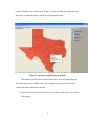
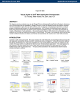
In this project a tool has been developed to display interactive cartographic maps
for the state of Texas. The maps interactively provide various demographic data for the
state of Texas. This tool can be used by any user for the purpose of comparing different
census data across different counties for the state of Texas.
This project was developed as a three tier application with a geospatial database
as the data source/data provider, a middle business/logic layer which consumes the data
and does the data transformation, and a user interface layer that displays the generated
interactive maps to the user. The software displays interactive maps with demographic
information for the state of Texas. The software provides county wide information on
population, population density, number of housing units, and male/female ratios. Detailed
information about each county can be obtained just by the click of a button.
The software provides additional functionality to import shapefiles into a
geospatial database and to display the same as maps. These maps can be added as layers
one over the other. So two different shapefiles can be imported and can be seen as a
single map by adding two different vector layers. The user is allowed to add any column
from the database as a label over the map thus providing functionality for easy data
visualization.
The project was developed using Microsoft Visual Studio 2005 as the IDE. Visual
Basic .net was used as the programming language. PostgreSql was used as the database.
PostgreSql was chosen because of its support for the geospatial databases. ArcMap was
used to create shapefiles for the state of Texas with the related demographic data.
ii
TABLE OF CONTENTS
Abstract………………………………………………………………………………........ii
Table of Contents…………………………………………………………………………iv
List of Figures…………………………………………………………………………….vi
List of Tables…………………………………………………………………………….vii
1.
Introduction and Background...………………………………………………………1
1.1
GIS and Cartographic Visualization..………………………………………......1
1.2
Cartographic Visualization…..…………………………………………………2
1.3
Geodatabases…………………………………………………………………...3
1.3.1
1.4
Representation of a Geodatabase……………………………………..4
Existing System………………………………………………………………..5
1.4.1
Problems with the Existing System………………………………......6
1.5 Project Goals………………….………………………………………………….6
1.6 Project Report Organization……………………………………………………...7
2.
Cartographic Visualization for the State of Texas…………………………………...8
2.1
3.
Interactive Maps with Census Data…….……………………………………..8
2.1.1
Thematic/Gradient Maps………….………………………………….11
2.1.2
Maps with Pie Charts….………….…………………………………..12
2.2
Converting Shapefiles to Geospatial Data..…………………………………..13
2.3
Creating New Maps……………….………………………………………….15
System Design…………..………………………………………………………….18
3.1
Geodatabase Design…...……………………………………………………...18
3.1.1
PostgreSql……………………………………………………………20
iii
3.1.2
3.2
Design and Implementation………………………………………….20
User Interface Design...………………………………………………………23
3.2.1
Design and Implementation…………………………………………..24
3.2.1.1 App.Config File……………………………………………..24
3.2.1.2 GenerateMaps.vb……………………………………………25
3.2.1.3 Shape2Spatial.vb…………………………………………….26
3.2.1.1 DbSettings.vb………………………………………………..26
4. Testing and Evaluation……………………………………………………………...27
4.1
Functional Testing…………………………………………………………...27
4.2
Usability Testing……………………………..………………………………29
5. Future Work…………………….…….……………………………………………...30
6. Conclusion…………………….…….…………………………………………….....31
Bibliography and References…………………………………………………………….32
Appendix A: Application Configuration Settings…………...…………………………...34
Appendix B: Sample Use Case…………………………………………………………..36
Appendix C: Class Diagrams…...………………………………………………………..37
Appendix D: User Manual……...………………………………………………………..40
iv
LIST OF FIGURES
Figure 1.1 Polygon dataset depicting the frequency of fires..…………………………….4
Figure 1.2 Thematic raster dataset………………………………………………………...4
Figure 1.3 Geodatabase architecture.……………………………………………………...5
Figure 2.1 Interactive map showing census data...………………………………………..9
Figure 2.2 Detailed census data..……………………….………………………………..11
Figure 2.3 Thematic map showing population density..……………...………………….12
Figure 2.4 Map with pie chart showing male/female ratio...………...…………………..13
Figure 2.5 Data conversion tool..……………………...……………...………………….14
Figure 2.6 Data preview pane………………………………………...………………….15
Figure 2.7 Add new map..……………………………..……………...………………….16
Figure 2.8 Results of adding a new map...…………….……………...………………….17
Figure 2.9 Resulting map after adding a new rivers layer….....……...………………….17
Figure 3.1 Stages of a geodatabase design…...…………………………………………..19
Figure 3.2 Data processing and loading……………………………………………….....22
Figure 3.3 Design of the application….………………………………………………….23
v
LIST OF TABLES
Table 3.1 Application and User Settings in App.Config file…………………………….25
Table 3.2 Methods in the GenerateMaps.vb Class.……………………………………...26
Table 4.1 Functional Testing Results………………………...…………………………..28
Table 4.2 Usability Testing Results………………………….…………………………..29
vi
1.
INTRODUCTION AND BACKGROUND
Maps are simplified representations of reality. This partly is done for convenience
since it becomes very difficult to draw and interpret multiple information themes on one
map covering more than a very small area. Before computers became widely available,
thematic maps on plastic Mylar sheets could be laid on top of each other, revealing more
information about an area than was possible with any single paper map. The amount of
data that could be represented on such maps was very limited and also there was no way
to link the information related to the map to the map itself [James 2001].
Currently there is no existing application for the custom specific settings of the
proposed Texas census geodatabase and cartographic visualization. Recently a project
titled “Design and Implementation of a User Friendly Geodatabase System for the State
of Texas” [Uppala 2006] has been implemented which retrieves the population data from
a database and presents it as reports rather than having it on a map so that users can
visualize and interact with it. Demographic data when presented as interactive maps can
provide more information to the user both for informational and data analysis purpose.
In order to use the program designed in this project one does not need to know
ArcGIS. The designed program makes it easy to map data for the state of Texas.
1.1 GIS and Cartographic Visualization
A geographic information system (GIS) is an information management system for
archiving, retrieving, analyzing, and visualizing data referenced by spatial or geographic
coordinates. A GIS acts as an integrating technology that helps to store and retrieve
information based on where they are physically located [Anderson 2003]. GIS technology
1
incorporates common database operations with the unique visualization and spatial
analysis advantage offered by maps.
GIS has evolved out of a long tradition of map making. Over the years GIS has
evolved through multiple parallel but separate applications across numerous disciplines.
Maps are simplified representations of reality. This partly is done for convenience since it
becomes very difficult to draw and interpret multiple information themes on one map
covering more than a very small area.
The development of the Geographic Base File/Dual Independent Map Encoding
(GBF-DIME) files by the U.S. Census Bureau in the 1960s marked the large-scale
adoption of digital mapping by the government [GISHISTORY 1997]. A grid-based
mapping program called SYMAP [Chrisman 2004], developed at the Laboratory for
Computer Graphics and Spatial Analysis at the Harvard Graduate School of Design in
1966, served as a model for later systems [Chrisman 2005]. These early GIS packages
were often written for specific applications and required the mainframe computing
systems found usually in government or university settings. In the 1970s, private vendors
began offering off-the-shelf GIS packages. M&S computing (later Intergraph) and
Environmental Systems Research Institute (ESRI) emerged as the leading vendors of GIS
software [James 2001].
1.2 Cartographic Visualization
Cartography plays an important role in the graphical presentation of geospatial
information. The cartographic visualization process involves translation or conversion of
geospatial data from a database into maps applying cartographic methods and techniques.
2
In other words principles from cartography and geographic information systems are
integrated in the development and presentation of georeferenced information.
Translation of data from a geospatial database and presenting it as a graphical
map is the most efficient and effective means of presenting the data to the user.
Presenting data as maps enables the user to locate geographic objects on the map.
Different colors, shapes, and signs can be used to inform the user about the characteristics
of a particular place on a map, i.e. a location on the earth.
Cartographic maps were designed by taking into account the information that can
be presented through the maps, since the nature of the data determines the graphic
options. For example, a gradient map with different colors can be used when presenting
data like population density while lines of different types can be used to represent rivers
and roads.
1.3
Geodatabases
A geodatabase is a storage mechanism for spatial and attribute data. It contains
collection of features, attributes and, relationships between features. All geodatabases,
whether personal or ArcSDE can store tables, feature classes, feature datasets and so on.
Geodatabases are grouped into two different types: vector and raster. Vector data
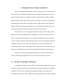
is represented using points, lines and polygons [GISLOUNGE 2005a]. Figure 1.1 is an
example of polygon dataset with thematic color mapping.
3
Figure 1.1 Polygon dataset depicting the frequency of fires [GISLOUNGE 2005a]
Raster data is represented as a surface divided into a regular grid of cells. There
are three types of raster datasets: thematic data, spectral data, and image data
[GISLOUNGE 2005b]. Figure 1.2 is an example of a thematic raster dataset also called a
Digital Elevation Model (DEM).
Figure 1.2 Thematic raster dataset [GISLOUNGE 2005b]
1.3.1 Representation of a Geodatabase
The geodatabase provides the common data access and management framework
for ArcGIS that enables us to deploy GIS functionality and business logic wherever it is
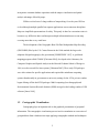
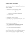
needed in desktops, servers, or mobile devices [ESRI 2005]. Figure 1.3 represents the
geodatabase architecture. With this architecture the user has the tools to assemble data for
geographic information systems [ESRI 2005]. The geodatabase is a common framework
shared by all ArcGIS products and applications.
4
Figure 1.3 Geodatabase architecture [ESRI 2005]
1.4
Existing System
A Project titled “Design and Implementation of a User Friendly Geodatabase
System for the State of Texas” [Uppala 2006] has been implemented which retrieves the
population data from a database and presents it as reports. The application is data driven
and all the data is stored and retrieved from a database. The application presents a
clickable map for the state of Texas which can be used to update and retrieve the required
information. The information for each county can be retrieved and updated by clicking on
the respective county of the map.
5
1.4.1
Problems with the Existing System
The existing system retrieves the population data from a database and presents it
as reports. Any census data presented in the form of reports is hard to visualize and
comprehend. Census data can be easily visualized when presented on the map. This also
helps in comparing the data for the various regions of the map.
Comparing census data between the different regions becomes difficult when the
information is presented as reports. If a comparison has to be made then data for each
region to be compared has to be either saved to files or printed out before comparing.
This is difficult but possible if there are only few regions to compare but when all the
data across the state has to be compared this becomes impossible.
1.5
Project Goals
The major goal of the project is to present data extracted from a geospatial
database in the form of interactive maps. In order to realize this goal a number of
preliminary steps have to be performed including converting and loading data into the
database. The following goals have been realized.
•
Convert and load data from shapefiles into a data format that can be stored in a
geospatial database.
•
Read the data from the database and present it as interactive maps with data from
the database.
•
Allow the user to create any map on the fly with data retrieved from the database.
•
Allow the user to add vector layers to a map with data obtained from different
data sources and presenting all the information in a single map.
6
1.6 Project Report Organization
The next section (Section 2) presents the narrative of the scope and
accomplishments of the project. Section 3 presents the design and implementation of the
project, including database design and implementation of the user interface. Section 4
discusses the testing procedures adopted to test the project for any bugs. A discussion of
future work related to this project is discussed in section 5. Section 6 includes the
conclusions derived from this project.
7
2.
CARTOGRAPHIC VISUALIZATION OF CENSUS DATA FOR
THE STATE OF TEXAS
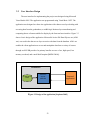
Cartographic Visualization for the State of Texas is a windows forms application
designed using Visual Studio .net 2005. The two main components of the project are a
geospatial database designed and implemented in PostgreSql, and a front end to present
the data as maps. The project utilized GIS technologies in creating census datasets for
state of Texas. The front end user interface of the project has three major components:
•
Interactive map for the state of Texas that shows census data for the state of
Texas.
•
Data upload tool that helps convert any kind of shapefile into a format that can be
stored to a spatial database. This data can be later used to generate maps on the
fly.
•
Maps can be generated on the fly from the data stored in the database. Data from
different tables can be added as layers and can be seen on a single map allowing
us to combine data from various sources into a single map.
2.1
Interactive Maps with Census Data
This part of the project focused on creating an interactive map for the state of
Texas. The map shows county wise census data. Data like total population, population
density, and number of housing units are shown for each county. In addition functionality
is provided to create thematic maps for showing population density, and number of
housing units in each county. Maps with pie charts are also provided to show such ratios
8
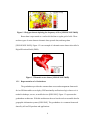
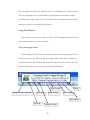
as male to female ratios in each county. Figure 2.1 shows a simple map with census data
that shows up when the mouse is moved over any particular county.
Figure 2.1 Interactive map showing census data
The software provides various controls to the user to view and change the map.
The following tools are available to the user to control how the map is shown and to
control what data is displayed on the map.
•
Zoom In: The Zoom In control lets the user to zoom in to the map to see each area
more clearly.
9
•
Zoom Out: The Zoom Out control lets the user make the map smaller. When a
user zooms in if the map is too big then he/she can use the Zoom Out tool to make
the map smaller.
•
Zoom to Extents: This tool can be used to redraw the map to its original size.
•
Pan: Panning is bringing a particular area of the map into focus. The map can be
panned by right clicking and dragging the map to any location.
•
Show/Hide Labels: These tools can be used to show or hide the county names on
the map.
•
Show/Hide Tooltip: Census data for each county is displayed as a tooltip. This
tooltip can be shown or hidden using these controls.
•
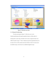
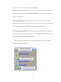
Detailed Data: Double clicking on any county brings up a new screen that shows
the census data and various graphs for that particular county. Figure 2.2 shows
detailed data view for Nueces County.
10
Figure 2.2 Detailed census data
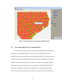
2.1.1 Thematic/Gradient Maps
The links on the right in Figure 2.1 allow the user to access
thematic/gradient maps showing the population density, and the number of
housing units in each county. Such data can be used to compare the data across
different counties. Figure 2.3 shows a thematic map for the population density for
the state of Texas. All the controls such as the Zoom in, Zoom out, and access to
the detailed county wise data are also available through these maps.
11
Figure 2.3 Thematic map showing population densities
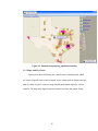
2.1.2 Maps with Pie Charts
Data such as the male/female ratio, and the ratio of housing units which
are owner occupied versus renter occupied versus vacant units are shown on maps
with pie charts. Figure 2.4 shows a map with the male/female ratios for various
counties. The map in the figure has been zoomed in to show the graphs clearly.
12
Figure 2.4 Map with pie charts showing male/female ratios
2.2
Converting Shape Files to GeoSpatial Data
The software has a built-in tool to convert any given shapefile to a format that can
be imported into a geospatial database. The user needs to specify the name of the
shapefile to be converted and the name of the destination database. The software creates a
new table in the user specified database with the same name as the shapefile and import
all the relevant data into that table. A new table is created for every shapefile imported.
The user needs to have permissions to create new tables in the specified database. The
connection to the database with the user credentials can be tested before proceeding
further. The software provides the user with tools to preview the data in the shapefile so
13
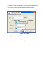
that the user can know beforehand what is being imported. Figure 2.5 shows the data
conversion tool in action.
Figure 2.5 Data conversion tool
After previewing the data the user can click the ‘Upload to Database’ button to
start the conversion and import process into the database. After the data has been
successfully imported the user can open the data from the tool as if he/she has opened the
14
newly created table in the database. Figure 2.6 shows the table after the data has been
imported into the database.
Figure 2.6 Data preview pane
2.3
Creating New Maps
Data imported in the previous section can be used to create new maps. Labels
specifying the map regions or any other labels can be added to the map by specifying the
columns in the database tables. New Vector layers can be added to the existing maps thus
creating a map with the required details. For example a shapefile with country boundaries
can be converted to geospatial data and can be added as a new map and another layer
with data about the rivers can be added as a vector layer to the map thus creating a new
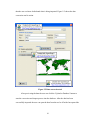
map which shows all the rivers in the world. Figure 2.7 shows the process of adding a
new map. After specifying the database settings, clicking on the ‘Retrieve Tables’ button
retrieves all the existing tables in the database. The user can then select any table that
15
he/she wishes to add as a new map. If the user wishes to add labels to the map the user
needs to specify the column whose data will be used as labels over the map.
Figure 2.7 Add new map
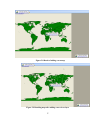
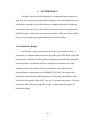
Figure 2.8 shows the result of adding a new map. Controls can be used to Zoom
In and Zoom Out and perform other operations. Figure 2.9 shows the same map with a
new vector layer with rivers data added to the map.
16
Figure 2.8 Result of adding a new map
Figure 2.9 Resulting map after adding a new rivers layer
17
3. SYSTEM DESIGN
A Windows forms based GIS application for creating and displaying interactive
maps with Texas census data was developed in this project. The system incorporates GIS
and database technologies to provide an interactive mapping application for displaying
census data for the state of Texas. The software also provides tools to convert data from
shapefile format to a format that can be stored in a database. Finally the software enables
the user to create maps from geospatial data retrieved from the database.
3.1 Geodatabase Design
The first phase of the project involved the design of a geodatabase system. A
geodatabase is a relational database that stores geographic data [ESRI 2005b]. It may thus
be described as a container for storing spatial and attribute data and the relationships that
exist among them. A geodatabase provides a technique for representing real world
geographic features and attributes as objects in a database, and is hosted inside a
relational database management system (RDBMS) [Zeiler 2004]. The design of the
geodatabases generally starts with the thematic layer. Designing a geodatabases can be
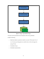
divided in to three phases [Arctur 2005]. They are 1) Conceptual design phase, 2) Logical
design phase and 3) Physical design phase. Figure 3.1 illustrates the three phases of
Geodatabase design.
18
Conceptual Phase
Logical Design Phase
Physical Design Phase
Geodatabase
Figure 3.1 Stages of geodatabase design
The major activities performed in the development of the census geodatabase
include the following:
•
Identify the database system that is suitable to store the GIS data and is free of
cost. For this project PostgreSql was a suitable choice with its rich support for
storing GIS data.
•
Geodatabase Design.
•
Geodatabase Implementation.
19
3.1.1 PostgreSql
PostgreSql was used as the geospatial database in developing this project.
PostgreSql is an open source Relational Database Management System (RDBMS).
PostgreSql has rich object oriented features such as inheritance, polymorphism and the
ability to create complex user defined datatypes. PostgreSql has the built-in ability to
process the spatial datatypes, called geometry or feature. All these features make
PostgreSql an ideal candidate for storing and retrieving geospatial data. In order for
PostgreSql to store GIS related spatial data an extension called PostGIS has to be added
and enabled in PostgreSql. PostGIS adds support for geographic objects to the PostgreSql
object-relational database. In effect, PostGIS creates a spatially enabled PostgreSql
server, allowing it to be used as a backend spatial database for GIS.
3.1.2 Design and Implementation
The census data has two principal components. They are geographic mapping data
of the physical features and tabular population data. Once the data is obtained, then
managing, correcting and updating the collected data are major tasks. Because of the
extensive use of census data both by private and public organization, the data model was
developed to enable the user to put the data to maximum use. The main design issues of
the census data model were designing the thematic layer framework, geodatabases
structure, census topology, rules for the census topology, census boundaries, linking
census demographic statistics, and deciding on the administrative units.
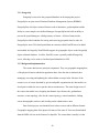
Data for this project was obtained from various sources and in different formats.
Geographic mapping data of the physical features of the state of Texas was downloaded
from the ESRI web site in the format of a shapefile. The census data is usually is in the
20
form of tabular format. Census data was obtained in summary file format from the ESRI
web site. The two sets of data were merged using ArcMap software to create a new
shapefile. Figure 3.2 shows the process of obtaining and loading the census data into the
GIS database. The following steps were performed in ArcMap to create a new shapefile:
•
The shapefile with data of the county boundaries for the state of Texas was loaded
into ArcMap.
•
With the shapefile loaded the summary file with the demographic information
was loaded into ArcMap.
•
A join was preformed to join the demographic with the physical features for the
state of Texas. A join relates the attribute data in the table to the geographic data
layer by using a common attribute field.
•
The file was saved as a shapefile.
This newly created shapefile has all the required information and was imported
into the database with the data import tool that was developed as part of this project.
21
Shapefile with Physical features
Summary file with Census data
ArcMap
Software
(create a join)
New shapefile with both data
Data Import Tool
Database
Figure 3.2 Data processing and loading
22
3.2
User Interface Design
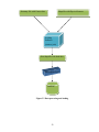
The user interface for implementing the project was designed using Microsoft
Visual Studio 2005. The application was programmed using Visual Basic .NET. The
application was designed as a three tier application with a data access layer dealing with
accessing data from the geodatabase, a middle logic/business layer transforming and
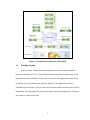
computing data to a format suitable for display by the front end user interface. Figure 3.3
shows a basic design of the application. Microsoft® ActiveX® Data Objects .net (ADO
.net) was used in the data access layer to retrieve the data from the database. ADO .net
enables the client application to access and manipulate data from a variety of sources
through an OLE DB provider. Its primary benefits are ease of use, high speed, low
memory overhead, and a small disk footprint [MSDN 2004a].
Geodatabase
Data
Database
access
software
Front-end
Application
Figure 3.3 Design of the application [Stephens 2002]
23
3.2.1 Design and Implementation
This section discusses the technical details of the code implementation. Various
classes that are used for data access, generating maps, storing, and retrieving user settings
etc. are discussed. This discussion focuses mainly on the functionality of core classes.
3.2.1.1 App.Config File
Microsoft .net environment provides an easy way to store and retrieve application
and user settings. Application wide settings like the database connection strings, and user
settings like the color preferences, language etc. can be stored in a central repository file
called App.Config. Just a couple of lines of code is all that is needed to retrieve these
settings. While the application settings are Read-Only, the user settings can be written to
thus allowing the application developer to store any user preferences in the App.Config
file.
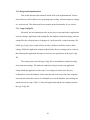
The current project uses the App.Config file to store database connection string
and certain user settings. The database connection string is stored as an application
setting which has application wide scope. User settings are used to store the user
credentials to access the database. Since more than one user can use the same computer
and each user has his/her own set of credentials to access the database, these settings are
stored with a user scope. Table 3.1 shows the application and the user settings stored in
the App.Config file.
24
Table 3.1 Application and User settings in App.Config file
Setting
Scope
Value
ConnString
Application
Driver={PostgreSql};Server=127.0.0.1;Port=5432;
Database=GisDb;Uid=Reena;Pwd=*****;
Database
User
GisDb
Port
User
5432
Server
User
Localhost
UserName
User
Password
User
The code fragment below shows a way to access the ConnString application
settings stored in the App.Config file:
Dim Connection as string ‘ declare a variable as string
Connection = My.Settings.ConnString ‘ read value from App. Config
3.2.1.2 GenerateMaps.vb
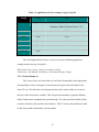
This is one of the core classes that are vital for the functionality of the application.
GenerateMaps.vb class is designed to create interactive maps with census data for the
state of Texas. This class has several properties that can be used to either set or retrieve
that any of the class private variables. This class provides methods to generate different
kinds of maps and to manipulate the generated maps. The class provides methods to hide
and show the labels, hide and show the tooltip etc. Table 3.2 shows the methods provided
by this class and the functionality of each method.
25
Table 3.2 Methods available in the GenarateMaps.vb Class
Method Name
Function
InitializeMap
Creates a new empty map
AddLabels
Adds labels showing the map regions
GetLabelLayer
Return the label layer
GradientMap
Creates a thematic map
Male/femaleRatioChart
Create a map with pie charts showing
male/female ratio
Create a map with housing ratios
HousingRatioChart
3.2.1.3 Shape2Spatial.vb
This class is used to convert any shapefile to a data format that can be imported
into a GIS database. This class uses the GenerateMaps.vb class to generate a preview
map from the shapefile.
3.2.1.4 DbSettings.vb
This class is used to gather the database information from the user when the user
wants to create a new map. This Class exposes a public event that is raised after the user
has finished entering all the required information. This event is caught in the calling class
and necessary steps are taken to generate a new map.
26
4.
TESTING AND EVALUATION
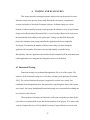
This section describes testing procedures employed to test the project for errors.
Software testing is the process used to help identify the correctness, completeness,
security and quality of developed computer software. Software testing is a critical
element of software quality assurance and represents the ultimate review of specification,
design and code generation [Pressman 2001]. A set of testing schemes were used to test
the functionality and usability of the application. Testing was done both during the
project development (unit testing) and after the application has been completely
developed. To minimize the number of defects unit testing was done during the
application development. Each part was tested individually to test the correct
functionality. Once the application has been developed completely all the individual parts
of the application were integrated and integration tests were performed.
4.1 Functional Testing
Functional testing was performed throughout the life cycle of the project. The
objective of the functional testing is to verify how well the system performs [Pressman
2001]. The various functions the project is supposed to execute were tested. User
commands, data manipulation tools, map generation, map navigation tools of the system
were tested. Any errors found during Functional testing were corrected before adding any
new features to the software.
The next phase of testing was functional verification testing that was done by the
users who were explained the scope and the functionality of the project. Five testers who
work at Computer Services at Texas A&M University-Corpus Christi were involved in
27
testing the application. The testers are computer savvy and have some programming
knowledge but none of the testers is knowledgeable about GIS related concepts. The
testers did not have knowledge of the internal workings of the applications but just what
the application is supposed to do and the expected results. During this test phase each of
the testers were assigned to test different functionality of the application. The testers were
provided with test cases that describe in detail what the tester needs to do and how to do
it. The test case also showed the expected outcome of the process. The tester then
performed the action and verified the outcome with the outcome described in the test
case. Any defects found were documented and fixed.
After all the defects found in the functional verification testing have been fixed,
the final phase of testing was performed. This was done to ensure that all the defects have
been fixed and also to ensure that the new fixes have not created any new bugs in the
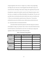
application. Table 4.1 shows the results of Functional testing.
Table 4.1 Functional Testing Results
Test Phase
Phase 1
Phase 2
Module Tested
Number of Test Cases
Number of Defects
Texas Census
8
2
Data Conversion
4
0
New Maps
10
2
Texas Census
8
0
Data Conversion
4
0
New Maps
10
1
28
4.2 Usability Testing
Usability testing is used to identify how users actually interact with the
application. The application was tested for the ease of navigation through the forms,
appearance, and consistency.
Appearance: All the forms were checked for the uniformity in the appearance.
Ease of navigation: The application was tested to see if there are any links that break the
application and made sure that all the links are properly connected to the required pages.
Consistency: The application was tested for the consistency of the data that is being
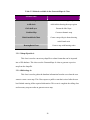
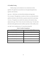
displayed on the pages. Table 4.2 shows the results of usability testing. The results in the
table show that the application meets the usability requirements. All the usability criteria
were rated 5 out of a maximum score of 5 except for the look and feel.
Table 4.2 Usability Testing Results
Usability Metric
Score (Out of 5)
Ease of Use
5
Look and Feel
4
Colors and Fonts
5
Ease of Navigation
5
Features
5
29
5. FUTURE WORK
This project has some scope for enhancement in the future. The following are
some of the ideas that can be incorporated into this project in future.
• Data: More data need to be presented in an easy to present manner. Presenting a
lot of data on a map clutters the map defeating the main purpose. A better way
needs to be implemented to show all the available data for a given map.
• Charts: The look and the information presented on the Pie charts shown on the
maps have to be improved. New features can be implemented to increase size of
the chart to a certain extent when zooming in to the map.
• User Preferences: There is a scope to allow the user to select the background
colors for each map and the colors for the new layers and labels.
30
6.
CONCLUSION
The design of the project is aimed at understanding the design principles and
practices involved. The software can be used to view the census data for the state of
Texas in an interactive manner. The software provides the user with a lot of flexibility in
viewing and analyzing the census data. Population densities and the number of housing
units across different counties can be compared by the click of a button. Detailed census
data for a desired county is only a button click away.
The software provides a tool to convert any shapefile into a format that can be
stored in a GIS database. This will help the available data to more use. Also new maps
can be generated from different shapefiles imported into the GIS database.
31
BIBLIOGRAPHY AND REFERENCES
[Anderson 2003] Anderson, S. J. and Harmon, J. E. The Design and Implementation of
Geographic Information Systems. John Wiley & Sons, Inc. Hoboken, New Jersey,
2003.
[Arctur 2005] Arctur, D. and Zeiler, M. Designing Geodatabases. ESRI Press, 2004.
[Chrisman 2004] N. R. Chrisman, Charting the Unknown: How Computer Mapping at
Harvard became GIS, 2004.
http://gis.esri.com/esripress/shared/images/82/HarvardBLAD_screen.pdf (Visited
May 20, 2007).
[Chrisman 2005] Nicholas R. Chrisman, History of the Harvard Laboratory for
Computer Graphics: a Poster Exhibit, 2005.
http://www.acsm.net/cagis/chrisman-History.pdf (Visited May 22, 2007).
[ESRI 2005] Geodatabase. Available from
http://www.esri.com/software/arcgis/geodatabase/index.html (Visited May 21,
2007).
[ESRI 2005b] Environmental Systems Research Institute. Creating, Editing, and
Managing Geodatabases for ArcGIS 9. Available from
http://campus.esri.com (Visited May 26, 2007).
[GISHISTORY 1997] David M. Mark, Nicholas Chrisman, Andrew U. Frank, Patrick H.
McHaffie & John Pickles, The GIS History Project, 1997.
http://www.geog.buffalo.edu/ncgia/gishist/bar_harbor.html (Visited May 20,
2007).
[GISLOUNGE 2005a] Geodatabase explored. Available from
http://gislounge.com/features/aa050100a.shtml (Visited Mar 21, 2007).
[GISLOUNGE 2005b] Geodatabase explored. Available from
http://gislounge.com/features/aa050100b.shtml (Visited Mar 21, 2007).
[James 2001] Nathaniel James, History of GIS, Spring 2001.
http://envstudies.brown.edu/Thesis/2001/james/gishistory.html (Visited May 20,
2007).
[MSDN 2004a] ADO Data Access.
http://msdn.microsoft.com/library/default.asp?url=/library/enus/vbcon98/html/vbmscVisualBasicDocumentationMap.asp (Visited May 21,
2007).
32
[Pressman 2001] Pressman, R. Software Engineering: A Practitioner’s Approach.
McGraw-Hill, New York, 2001.
[Stephens 2002] Rod Stephens, Visual Basic .NET Database Programming. QUE April
11, 2002.
[Uppala 2006] Uppala, A. Design and Implementation of a User Friendly Geodatabase
System for the State of Texas, Graduate Project, 2006.
[Zeiler 2004] Zeiler, M. and Arctur, D. Designing Geodatabases: Case Study in GIS
Data Modeling. ESRI Press, Redlands, Calif., 2004.
33
APPENDIX A – APPLICATION CONFIGURATION SETTINGS
<?xml version="1.0" encoding="utf-8" ?>
<configuration>
<configSections>
<sectionGroup name="applicationSettings"
type="System.Configuration.ApplicationSettingsGroup, System, Version=2.0.0.0,
Culture=neutral, PublicKeyToken=b77a5c561934e089" >
<section name="TexasDemographics.My.MySettings"
type="System.Configuration.ClientSettingsSection, System, Version=2.0.0.0,
Culture=neutral, PublicKeyToken=b77a5c561934e089" requirePermission="false" />
</sectionGroup>
<sectionGroup name="userSettings"
type="System.Configuration.UserSettingsGroup, System, Version=2.0.0.0,
Culture=neutral, PublicKeyToken=b77a5c561934e089" >
<section name="TexasDemographics.My.MySettings"
type="System.Configuration.ClientSettingsSection, System, Version=2.0.0.0,
Culture=neutral, PublicKeyToken=b77a5c561934e089"
allowExeDefinition="MachineToLocalUser" requirePermission="false" />
</sectionGroup>
</configSections>
<system.diagnostics>
<sources>
<!-- This section defines the logging configuration for My.Application.Log -->
<source name="DefaultSource" switchName="DefaultSwitch">
<listeners>
<add name="FileLog"/>
<!-- Uncomment the below section to write to the Application Event Log -->
<!--<add name="EventLog"/>-->
</listeners>
</source>
</sources>
<switches>
<add name="DefaultSwitch" value="Information" />
</switches>
<sharedListeners>
<add name="FileLog"
type="Microsoft.VisualBasic.Logging.FileLogTraceListener,
Microsoft.VisualBasic, Version=8.0.0.0, Culture=neutral,
PublicKeyToken=b03f5f7f11d50a3a, processorArchitecture=MSIL"
initializeData="FileLogWriter"/>
<!-- Uncomment the below section and replace APPLICATION_NAME with the
name of your application to write to the Application Event Log -->
<!--<add name="EventLog" type="System.Diagnostics.EventLogTraceListener"
initializeData="APPLICATION_NAME"/> -->
</sharedListeners>
34
</system.diagnostics>
<applicationSettings>
<TexasDemographics.My.MySettings>
<setting name="ConnString" serializeAs="String">
<value>server=127.0.0.1;database=GisDb;User
Id=Reena;password=medha</value>
</setting>
<setting name="OledbConn" serializeAs="String">
<value>Driver={PostgreSql};Server=127.0.0.1;Port=5432;Database=GisDb;Uid=Reena;
Pwd=vijithar;</value>
</setting>
</TexasDemographics.My.MySettings>
</applicationSettings>
<userSettings>
<TexasDemographics.My.MySettings>
<setting name="Server" serializeAs="String">
<value />
</setting>
<setting name="Port" serializeAs="String">
<value>5432</value>
</setting>
<setting name="Database" serializeAs="String">
<value />
</setting>
<setting name="UserName" serializeAs="String">
<value />
</setting>
<setting name="Password" serializeAs="String">
<value />
</setting>
</TexasDemographics.My.MySettings>
</userSettings>
</configuration>
35
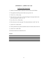
APPENDIX B – SAMPLE USE CASE
ToolTip and Label Functionality
1) Open the TexasDemographics Application from the shortcut on the desktop.
2) The Application should open with a blank texas map. Yes No
3) Click on View->Show tooltip
4) Move the mouse over the map. A tool tip should appear showing the data for that
particular geographic location. Yes No
5) Now click on View->Hide tooltip.
6) Move the mouse over the map again. The tooltip should not be visible. Yes No
7) Click on View->Show Labels
8) The map should now be generated with labels shown for all the counties. Yes No
9) Click on View->Hide Labels
10) The labels should now be hidden Yes No
Remarks
36
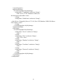
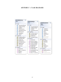
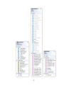
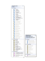
APPENDIX C – CLASS DIAGRAMS
37
38
39
APPENDIX D – USER MANUAL
Installation Instructions
The following are the main steps in installing and configuring the software.
•
Install and Configure the database
•
Populate the database.
•
Install and configure the software.
Installing and Configuring the Database
Installation:
1. Use the CD provided and browse to the folder called Postgre and start the
installation or Download the install for the Windows platform from the
PostGreSQL Binary Download ( http://www.postgresql.org/ftp/binary/ ) .
2. Make sure to check the PostGIS Spatial Extensions option, PgAdmin III, psql,
option.
3. To access the database server from other than the local machine itself Check the
"Accept connection on all addresses, not just localhost". This can be changed by
editing the postgresql.conf -> listen_addresses property. The default port of 5432
can also be changed as well in the postgresql.conf -> port property.
4. For language check PL/pgsql. If you forget, you can later use the createlang
plpgsql command to install in a specific database.
5. Enable contrib – Adminpack should be checked at the very least. This simplifies
adminstrative management of the server via PgAdmin III.
40
Creating and Populating a Spatial Database
PostGreSQL comes packaged with an admin tool called PgAdmin3. PgAdmin III
is under Start->Programs->PostGreSQL 8.2->PgAdmin III. Follow the steps below to
create a new spatial database.
•
Login with the userid and password set during install. Set the line
host all all 127.0.0.1/32 md5
to
host all all 127.0.0.1/32 trust
This will allow any person logging locally to the computer that
PostGreSQL is installed on to access all databases without a password.
(127.0.0.1/32) means localhost.
•
Create your database. Call it GisDb (case sensitive).
•
Use the PgAdmin III query tool to load the data into the GisDb database. To load
the data open the Data.sql file included in the CD and copy the lines and paste
them into the query tool and click on the ‘Run’ tool to populate the database.
Software Installation and Configuration
Use the CD to install the software. The installation should be pretty straight
forward. Follow the instructions on the wizard to install the software.
Once the software is successfully installed locate the file called
‘TexasDemographics.exe.config’. Use any text editor to open the file and locate the
line that says “ConnString”. This is the database connection information. Replace this
line with the appropriate values. The server value corresponds to the name or IP
address of the server on which the database was installed in the previous steps. The
41
Port corresponds to the port on which the server is configured to run. This typically is
5432 for PostgreSql server. UserId and Pwd correspond to the username and the
password used to log into the server. Save the file after the changes have been made
and you are ready to start using the application.
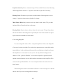
Using the Software
This software can be used to either view the Texas Demographic data in the form
of interactive maps or to create new maps.
Texas Demographic Data:
The first thing you notice when you open the software is an empty map of Texas.
From here you can view different data by using the links on the right. Controls are
provided to turn on and off labels and tooltip showing the data for each county. The
following figure shows the various tools and their functionality.
Hide Tooltip
Shapefile conversion tool
Zoom Out
Show Tooltip
Help
Show Labels
Hide Labels
Zoom In
Zoom to Extents
42
The same tools are also available in the menu control.
Zoom in and Zoom Out: These tools can be used to Zoom In to or out of the map. If
the map goes out of focus then the Zoom to Extents tool can be used to bring the
map to its original size.
Showing and Hiding Tool Tip: Tooltips show data as the mouse is moved over
each county. Data for each county is shown on the tooltip. This tooltip is available for
all the maps and can be turned off and on by using the Tooltip controls.
Showing and Hiding Labels: Labels show the names of the counties on the map.
This might get cluttered when the map is small. Showing and hiding of Labels can be
controlled using the Show/Hide Label controls.
Different maps for population density, Housing units etc. can be accessed by
clicking on the links to the right.
43
Population Density: Shows a thematic map of Texas with different colors indicating
different population densities. A legend is shown on the right side of the map.
Housing Units: Thematic map is shown with the number of housing units in each
county. A legend is shown on the right side of the map.
Male/Female Ratio: Map is shown with a pie chart for each county. The pie chart
indicates Male to Female ratio for each county.
Housing Ratio: Map is shown with a pie chart for each county. The pie chart shows
the ratio of number of housing units occupied by the owner to the number occupied
by the renter to the number of vacant units.
Converting Shapefile:
To convert shapefile click on File -> Import Shapefile or Click on the ‘Shapefile
Conversion’ tool in the toolbar. You need to have permissions to create tables in the
target database. In the resulting window provide your database credentials and open
the shapefile to be converted. You can preview the map before loading into the
database. Click ‘Upload to Database’ to convert the shapefile to spatial data and
upload it into the database. A new table with the same name as the shapefile will be
created in the specified database. To view the imported data click on the ‘Preview
Data’ button.
The data imported can be used with the software to create new maps or to add the
data as a new layer to an existing and relevant map.
44
Create New Maps:
New maps can be created and layers can be added to the new maps to visualize
data in the form of maps. Before a map can be created we need a shapefile with
relevant data. The shapefile has to be loaded into the database with the shapefile
conversion tool. Vector layers can be added to the newly created maps by clicking
the ‘Add Layer’ menu item from the ‘Tools’ menu.
45