Download DAN-WRELEASE 10 DYNAMIC ANALYSIS OF - CLARA-W

DAN-W RELEASE 10
DYNAMIC ANALYSIS OF LANDSLIDES
O. Hungr Geotechnical Research Inc., March 31, 2010
4195 Almondel Rd., West Vancouver, B.C., Canada, V7V 3L6
USER’S MANUAL
DAN-W
DYNAMIC ANALYSIS OF LANDSLIDES
O. Hungr Geotechnical Research Inc.
4195 Almondel Rd., West Vancouver
B.C., Canada, V7V 3L6
Tel. (604) 926-9129
© O. Hungr Geotechnical Research Inc. May, 2010
All rights reserved
______________________________________________________________DAN-W
TABLE OF CONTENTS
A
INTRODUCTION ...................................................................................................... 1
A.1
Purpose and limitations....................................................................................... 2
A.2
Calibration approach........................................................................................... 3
A.3
Additional precautions for use ............................................................................ 3
A.4
Problem size limits.............................................................................................. 5
B PROGRAM ORGANIZATION ................................................................................. 6
B.1
Installation of the program.................................................................................. 7
B.2
Program layout.................................................................................................... 7
B.3
Coordinate system............................................................................................... 7
B.4
2D / 3D configurations........................................................................................ 8
B.5
Opening and saving data files ............................................................................. 8
B.6
The main menu ................................................................................................... 8
C DATA INPUT........................................................................................................... 11
C.1
Data preparation................................................................................................ 12
C.2
Problem geometry setup ................................................................................... 13
C.3
New file sequence ............................................................................................. 13
C.4
Control parameters screen................................................................................. 14
C.5
Material properties screen................................................................................. 16
C.6
Material locations screen .................................................................................. 18
C.7
Edit path/top screen........................................................................................... 19
C.8
Edit width screen............................................................................................... 22
C.9
Options Screen .................................................................................................. 22
D ANALYSIS............................................................................................................... 26
D.1
Graphics ............................................................................................................ 27
D.2
How to run an analysis...................................................................................... 28
D.3
Run control box................................................................................................. 29
D.4
Analysis options................................................................................................ 30
D.5
Model instability ............................................................................................... 31
E DATA OUTPUT....................................................................................................... 33
E.1
Report................................................................................................................ 34
E.2
Output data........................................................................................................ 35
E.3
How to create ASCII graph files....................................................................... 36
E.4
ASCII graph file types ...................................................................................... 37
E.5
Observation point.............................................................................................. 41
APPENDIX 1, THEORY ............................................................................................... 44
APPENDIX 2, REFERENCES ...................................................................................... 53
APPENDIX 3, LIST OF WARNINGS AND ERROR MESSAGES ............................. 56
______________________________________________________________DAN-W
A INTRODUCTION
1
______________________________________________________________DAN-W
A.1 Purpose and limitations
DAN-W is an MS Windows-based program used to model the post-failure motion of
rapid landslides. The basic premise of the analysis is that, as a result of sliding or other
failure, a pre-defined volume of soil or rock ("the source volume") changes into a fluid
and flows downslope, following a path of a defined direction and width. The mass can
entrain additional material from the path and eventually deposits, when it reaches slopes
that are sufficiently flat ("the deposition area").
The model implements a onedimensional Lagrangian solution of the equations of motion and is capable of using
several alternative rheological relationships.
IMPORTANT NOTICE: DAN-W is a tool suitable for estimating the runout behaviour
of landslides on the basis of specific data on geometry and material properties, supplied
by the program user. The results of the calculations are entirely dependent upon the data
provided by the user. Therefore, persons using the program to make runout estimates
should be geoscience professionals thoroughly familiar with landslides, soil and rock
material behaviour and rheology, who have studied recent research publications on
landslide dynamics, including the relevant references listed at the end of this manual.
The properties entered into the program should always be checked by back-analysis of
real landslide case histories, similar to the existing or potential landslide being studied.
The results of the analysis should never be relied on exclusively, but should be
interpreted carefully by a qualified person in the light of field observations, empirical
estimates, other analyses and appropriate judgment and experience.
DAN-W is based on shallow flow assumptions and is best suited to shallow mass
movements, where the flow thickness is at least an order of magnitude less than the
length of the moving mass and the movement vectors are approximately parallel with the
bed. Where this condition is not satisfied, the results should be viewed with caution.
The solution may be unstable in certain cases where the flow is deep, or where abrupt
changes of slope occur. Beginning with Release 9, issued in September, 2008, the
program implements a velocity-smoothing algorithm, which removes most (though not
all) instability problems. As a consequence of velocity smoothing, the solution results,
i.e. the degree of longitudinal spreading of the moving mass, are now somewhat
dependent on the time interval used in the solution.
The optimal time interval is now set automatically by the program. It can be changed by
the user, but this should only be done together with careful testing of the effects. If the
solution shows signs of instability such as the appearance of irregular or translatory
waves, the results should not be trusted. In many cases, such problems can be overcome
by using a smaller number of reference blocks (50 is the recommended standard), shorter
time interval or switching between vertical and normal geometry. (The normal geometry
is usually considered superior).
2
______________________________________________________________DAN-W
A.2 Calibration approach
DAN-W uses the "equivalent fluid" approach, as described by Hungr (1995) and used
implicitly by many other researchers, before and after 1995. The flowing mass of the
landslide is simulated as a mass of simple fluid which is always frictional internally, but
with a basal flow resistance developed according to one of several alternative simple
rheological models. The best-fitting rheological model and the associated parameters can
be determined by independent laboratory tests only in cases of small-scale laboratory
model landslides. Thus, verification testing was carried out by analysing laboratory
flume experiments using dry sand and viscous oil (e.g. Savage and Hutter, 1978, Hungr,
1995and 2008).
Full-scale natural or man-caused landslides involve complex rheologies, affected by soilwater interactions, gross heterogeneity, scale and rate effects, most of which are effects
not suitable for sampling and laboratory testing. The rheological properties of the
"equivalent fluid" can therefore only be determined by back-analysis of real landslide
precedents. The general approach is to back-analyse known cases and assess the
performance of the model in terms of runout distance, length of deposit, deposit thickness
distribution, flow duration and distribution of flow velocities, where known in the field.
Given the relative simplicity of the basal rheology relationships, it is feasible to select the
optimal model and parameters that can then be used for forward predictions, provided the
landslide under analysis is similar in scale and character to the calibration cases.
Generally, the model results are much less sensitive to the internal friction angle than to
the basal rheological parameters.
A further discussion of the calibration approach and some examples are given in
Paragraph 4.9 of Hungr et al. (2005, copy enclosed with program package).
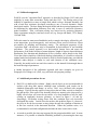
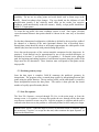
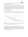
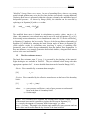
A.3 Additional precautions for use
ƒ
DAN-W is a shallow-flow solution. Highly curved slopes are not recommended for
analysis with deep slide masses, although some reasonably good results can be
obtained (Mancarella and Hungr, in review, 2010, copy enclosed with program
package). DAN-W has the option of using slices that are either vertical or normal to
the path profile. If the walls of the boundary blocks are normal to the slope profile, a
highly curved slope will cause the top surface of a deep landslide to loop on itself,
creating an apparently incorrect geometry, as shown in Figure 1 (a) and (b).
Surprisingly, verification testing shows that this condition does not necessarily
downgrade the results. Vertical slices do not have this problem (Figure 1c), however,
they may in fact be less accurate on steep slopes because the equations of motion are
in this case resolved in the horizontal direction. Where the problem exists, it is
recommended to run both configurations and take the more conservative result.
ƒ
As much as possible, the time step suggested by the program should be used. In some
instances, it is possible to eliminate instability problems by decreasing the time step
3
______________________________________________________________DAN-W
slightly, but using too small time steps may lead to "over-smoothing" and distortion
of the shape of the flowing mass. To speed up analysis, the user can select smaller
number of reference elements (although a warning will be issued if the number is less
than 50).
ƒ
DAN-W graphics do not implicitly show the decoupling of a slide mass when a
convex peak on a path is reached and one part of the mass flows forward while the
other lags upslope of the peak. Note that the model is not affected by this decoupling,
however the graphics are, so there is a straight line drawn between the two material
accumulations.
ƒ
Running the front of a slide mass a significant distance past the extents of the path
geometry can result in solution instability or inaccuracy. It is recommended that a
sufficient distance be included in the path profile to prevent flow beyond the extents.
ƒ
The equations of motion are developed in a one-dimensional framework, so there is
an implicit assumption that all resisting stresses arise only at the base of the flow,
while the flow depth is constant in the direction perpendicular to movement. Thus,
additional flow resistance that could be generated by the lateral flow boundaries in
highly confined flow paths is not accounted for. This should be kept in mind when
designing calibration programs: the back-analysis cases should have similar
confinement conditions as the case being analysed.
ƒ
Path Roughness: The input sequence in DAN-W requires the user to enter the path
geometry as a series of points, which the program fits by a spline function. The
spline appears during input or editing of the path geometry points and the user is
responsible to use just enough points to make the spline conform to the known path
geometry. The geometry input does not allow for overhags or sharp corners, which
would make the solution unstable. This need for smoothing precludes direct input of
x-y data into the program. Instead, the user should plot the path profile using a
graphics program, post the resulting image as a background image in the
Edit/Geometry screen and place sufficient points to correctly define the spline.
Please do not attempt to enter excessively complex geometry with intricate roughness
details: it will not improve accuracy and may make the solutions unstable. Ideally,
the path profile will be defined by 20 to 30 input points. The points should be evenly
distributed, except in places where it is necessary to force the spline to follow a sharp
change in angle.
ƒ
Defaults: Recent benchmark testing was carried out using default options as listed in
the Edit/Options/Analysis screen, namely: Time Interval (automatic), Smoothing
Coefficient (0.02), Tip Ratio (0.5), Stiffness Coefficient (0.05), Stiffness Ratio (5),
Centrifugal Forces (on), Trajectory (off), Boundary Block Geometry (normal) and
Lateral Stress Assumption (modified). It is recommended to keep these defaults for
routine analyses.
4
______________________________________________________________DAN-W
A.4 Problem size limits
ƒ
ƒ
ƒ
Maximum number of materials: 20
Maximum number of boundary blocks: 1000
Maximum number of geometry input points: 100
(a)
Vertical slices
Normal slices (same data)
(b)
Vertical slices
Normal slices (same data)
(c)
Figure 1: (a) An exaggerated example showing how the use of normal slices on a highly
curved slope can cause the slide mass to loop on itself. (b) A more practical example of
the above. (c) An example of how the mass elements become stretched in a steep-slope
problem that uses vertical slices.
5
______________________________________________________________DAN-W
B PROGRAM ORGANIZATION
6
______________________________________________________________DAN-W
B.1 Installation of the program
Run program setup.exe in the distribution folder. This will install DAN-W and its Help
Files in a chosen sub-directory on the hard drive. If setup does not work, it is sometimes
possible to start the program by double-clicking the DAN_Rel_10.EXE file. The user
may create a shortcut to DAN-W using Windows facilities. Run DAN-W through the
Start menu, or by double-clicking its name or shortcut. On starting, DAN-W presents a
title screen which disappears by clicking the mouse or any key on the keyboard. An
Initial Menu appears, prompting for one of two choices:
-
Create a new file
Open an existing file
IMPORTANT NOTE: While operating DAN-W on certain computers outside North
America, please do not forget to set your system to recognize dot, rather than comma, as
the decimal symbol. To do this, please go to Control Panel, Regional Settings.
B.2 Program layout
DAN-W has three main functions: data input, analysis, and data output. The data input
component allows the user to define the problem geometry, material properties, and
analysis options. Once the problem is defined, the user can run an analysis. Data is
collected during the analysis and can be output in various ways after the run is complete.
B.3 Coordinate system
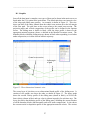
The main screen of DAN-W shows an isometric view of the slope profile and flowing
mass along the centre-line of the path. Horizontal distance, in metres, is shown from left
to right while elevation, also in metres, is shown from bottom to top. In the threedimensional configuration (default), the width of the channel is drawn in an isometric
view defined by a projection angle (see Section C.9).
During data input, the screen’s coordinate system changes depending on the data being
input. When inputting the slope and flowing mass’s profiles, the horizontal axis shows
horizontal distance from left to right, while the vertical axis shows elevation. When
inputting the path width, the vertical axis changes to width, in metres.
SLIDING DIRECTION:
It is important to note that the program was designed primarily for a sliding direction of
left to right. Therefore, a mass flowing from left to right will result in positive velocities
while a mass sliding from right to left will result in negative velocities. It is
recommended that the problem be described so that the sliding mass begins on the left
side and flows to the right of the screen.
7
______________________________________________________________DAN-W
B.4 2D / 3D configurations
DAN-W has a two-dimensional as well as a three-dimensional configuration. The twodimensional configuration works the same as 3D, except that the program assigns
constant 1m channel width. The three-dimensional configuration allows for a varying
channel width, assigned by the user along the length of the slope. To read about how to
change configurations, please refer to the Section C.4. For details on how channel width
is defined, refer to Section C.8, Section C.1, and Section D.1.
B.5 Opening and saving data files
Problems created in DAN-W can be saved under the file extension *.DNW. An ASCII
character file is saved containing all the input data, including problem geometry, material
properties, and material locations. Old files created in the DOS version of DAN (file
extension *.DAN) can be opened by DAN-W. However, some old data files may be
incomplete and all data should be checked.
To save a *.DNW file, choose the File-Save or File-Save As menu selection in the main
menu. To open a *.DNW file, choose the File-Open menu selection. To open a *.DAN
file, choose the File-Open .DAN menu selection.
B.6 The main menu
The program is controlled primarily through the Main Menu, which allows the user to
access the data input/edit screens, run an analysis, and control the output of data during
analysis. The Main Menu returns at the conclusion of each function. The following is a
list of all the options found in the Main Menu with a short description of each:
-
File: The items under this menu deal with file manipulation.
- File-New: Opens a new file with all the data either empty or set to a
default value. Also initializes the New-File Sequence (see Section C.3)
that guides the user through all the necessary data input screens.
- File-Open: Allows the user to open a previously saved *.DNW file.
- File-Open .DAN: Allows the user to open an old *.DAN file previously
created and saved in the DOS version of DAN.
- File-Save: Saves the current problem in the current directory and under the
current *.DNW file name.
- File-Save As: Allows the user to save the current problem in any available
directory as a *.DNW file.
- File-Exit: Ends and closes DAN-W.
8
______________________________________________________________DAN-W
-
-
Edit: The items under this menu allow the user to access the various data
input/edit screens as well as the options screen. This menu is enabled only when
a file is loaded.
- Edit-Control Parameters: Opens the Control Parameters Screen (see
Section C.4) which allows the user to input and modify the current file’s
identifying labels and problem boundaries, define the number of materials
and boundary blocks, set initial velocity and choose a cross-section shape
factor, a 2D or 3D configuration, end conditions and the uniform thickness
option.
- Edit-Material Properties: Opens the Material Properties Screen (see
Section C.5) which allows the user to choose the rheology of each material
and input/edit each material’s relevant properties. This screen also allows
the user to add and delete materials.
- Edit-Material Locations: Opens the Material Locations Screen (see
Section C.6) which allows the user to define where the various material
segments are located along the path profile.
- Edit-Path: Opens the Edit Path Screen (see Section C.7) which allows the
user to input/edit the slope profile.
- Edit-Top: Opens the Edit Top Screen (see Section C.7) which allows the
user to input/edit the initial flowing mass profile.
- Edit-Width: Opens the Edit Width Screen (see Section C.8) which allows
the user to edit the width of the channel. This item is only available in the
three-dimensional configuration.
- Edit-Options: Opens the Options Screen (see Section C.9) which allows
the user to change various boundary, display, and analysis options.
Solve: This menu accesses the analysis component of the program. It is enabled
only when a file is loaded. The selection activates the Run Control Box (see
Section D.3) which allows the user to run an analysis of the problem.
Output: The items under this menu deal with data output. This menu is enabled
only when a file is loaded.
- Output-Report: Displays a report (see Section E.1) summarizing the most
recent analysis.
- Output-Export ASCII Graph Files: Allows the user to choose at what time
intervals data is to be collected and placed into ASCII files (see Section
E.3).
- Output-Observation Point-View Data: Displays plots of the velocity and
the thickness of the sliding mass at a pre-specified location along the path,
as functions of time. This item is only available when the Observation
Point (see Section E.5) option is chosen in the Options Screen.
- Output-Observation Point-Export Data: Allows the user to export the
velocity and thickness data collected at the Observation Point to an ASCII
data file. This item is only available when the Observation Point option is
chosen in the Options Screen (see Section C.9).
- Output-Copy to Clipboard: Copies the current image on the main screen to
the clipboard. In the Depth-Profile mode, the two graphs shown are
9
______________________________________________________________DAN-W
-
-
separate images. To copy either of these graphs, click on the desired
graph and then select this menu option.
View: The items under this menu allow the user to change the main-screen view
from a three-dimensional isometric view of the problem to a two-dimensional
depth profile.
- View-Isometry: Displays in the main screen a three-dimensional isometric
view of the problem, as described in Section D.1.
- View-Depth Profile (2D): Displays in the main screen a two-dimensional
depth profile showing the sliding mass’s current velocity and thickness
distributions as functions of the horizontal distance, as described in
Section D.1.
- View-View Options: Gives rapid access to the ‘display’ portion of the
Options Screen (see Section C.9).
Help: Provides access to the DAN-W Help system.
10
______________________________________________________________DAN-W
C DATA INPUT
11
______________________________________________________________DAN-W
C.1 Data preparation
Before creating a data file for analysis in DAN-W, the user should be aware of the
following assumptions used by the model:
ƒ
ƒ
ƒ
ƒ
All geometry is two-dimensional. The slope and top surface profiles do not vary
in the transverse direction (perpendicular to movement). The path profile must be
constructed along the expected center-line of movement, even if curved in plan.
The direction of flow of the slide mass in the model is parallel to the plane of the
profile (i.e. from left to right of the screen).
The top surface geometry has a rectangular lateral cross-section defined by the
hydraulic depth of the slide mass and the channel width at that location along the
slope (see discussion of the Shape Factor, Section C.4.).
The slide mass is assumed to be a homogeneous “apparent fluid”. Its internal
strength is frictional, controlled by the "internal friction angle, φi". The basal
strength is determined by one of the several alternative rheological models. Both
the internal and external rheology may change along the length of the path.
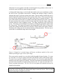
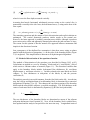
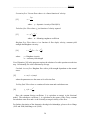
The first step is to prepare an elevation-distance slope profile, with two lines: the path of
the landslide and the ground surface defining the top of the unstable mass, in its original
position ("path and top" lines). The origin of the coordinate system should be in the
lower left corner of the screen, with the slope profile in the centre of the screen, as shown
in Figure 2. Data points containing elevation vs. horizontal distance along the slope from
the source to beyond the expected runout should then be chosen. True elevations can be
used, but the distance should start from 0 at the left corner.
Elevation, Z
A
(0 , 0)
B
Distance, Y
Figure 2: Vertical cross-section of a simple profile showing the layout of the coordinate
system and the position of the origin. Triangular data points represent the path and
circular data points represent the top of the slide mass in its original position. Points A
and B must be coincident on both lines. The path line can begin to the left of Point A, but
it is not recommended. Ideally, Point A (the crest of the source volume) should be the
first point on both the path and top lines.
12
______________________________________________________________DAN-W
IMPORTANT NOTE: The input profile should be made reasonably smooth to avoid
instability. Do not use too many points and avoid details such as minor steps in the
profile. Round out abrupt slope changes. The user should test the influence of such
simplification (usually it has relatively small effect on the results, but excessive
roughness could unrealistically reduce the runout). Ideally, a slope profile should have
about 15-25 input points.
To create the top profile, the same coordinate system is used. Once again, elevation
versus horizontal distance data points should be chosen in the same way as described
above.
For the three-dimensional configuration, width data is defined by the top-surface width of
the channel as a function of the same horizontal distance axis as described above.
Enough data points should be taken to sufficiently approximate the width profile of the
channel (they need not coincide with points defining the profile).
Next, data on the properties of the various materials encountered on the slope must be
prepared. Each material can be approximated by one of the provided rheologies, as
described in Section C.5 and Section A.5 of Appendix 1. If material varies along the
path, the beginning and ending locations of each material segment along the profile of the
slope must also be determined. These locations must correspond to data points on the
slope profile.
C.2 Problem geometry setup
Once the data input is complete, DAN-W constructs the problem’s geometry by
interpolation. The program creates a smooth slope profile by interpolating between data
points using the spline function. The top surface profile, on the other hand, is created by
linear interpolation between the data points. This surface is then split into the chosen
number of equally-spaced boundary blocks.
C.3 New file sequence
The New File Sequence, accessed through File-New in the main menu, or from the
startup screen, is a sequence of screens that guides the user through all the data input
steps that are required to create a new file. Once the sequence is complete and the user is
returned to the main screen, the problem is sufficiently defined to allow analysis to begin.
IMPORTANT NOTE: When the input or review of each data screen is complete, press
the menu item "Continue" to accept the data and, either continue the input sequence, or
return to the Main Menu.
13
______________________________________________________________DAN-W
The input sequence of screens is as follows:
1. Control Parameters screen.
2. Material Properties screen.
3. Edit Path/Top screen.
4. Edit Width screen (this screen is skipped if the 2D configuration was chosen in the
Control Parameters screen).
5. Material Locations screen (this screen is skipped if only one material was chosen in
the Control Parameters or Material Properties screens).
These screens can be visited individually after the sequence is finished. Note that the
Edit Path/Top screen cannot be exited until sufficient geometry data points are entered
for both the slope profile and the top surface. Also note that if the Cancel option is
chosen from the menus in the Control Parameters and Material Properties screens during
the New File Sequence, then the new file will be closed and exited without being saved.
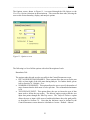
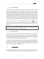
C.4 Control parameters screen
The Control Parameters screen, shown in Figure 4, is accessed through the Edit-Control
Parameters option in the main menu. It is also the first input screen in the New File
Sequence. This screen is used to input or edit the problem’s identifying labels, geometry
extents, and other parameters.
Figure 3: Control Parameters screen.
The following is a list of the input labels found on this screen and a description of each:
14
______________________________________________________________DAN-W
ƒ
ƒ
ƒ
ƒ
ƒ
ƒ
ƒ
ƒ
PROJECT: Optional. Any alphanumeric string of any length representing the
name of the project.
DATA SET: Optional. Any alphanumeric string of any length representing the
data set used in the project.
INPUT BY: Optional. Any alphanumeric string of any length representing the
user’s name.
DATE: Automatically updated to the system’s calendar. Can be changed to any
string.
UNIT WEIGHT OF WATER: Initially set to 9.81 kN/m3. All units are therefore
in SI metric units, including: metres (m), kilonewtons (kN) and kilopascals (kPa).
The Imperial units option is disabled in this version of DAN-W.
NUMBER OF MATERIALS: The number of materials or rheologies used in the
problem. There must be at least one material. The maximum number of materials
is 20. Please remember that materials other than number 1 will only be used, if
they are specified in the Material Locations screen.
NUMBER OF ELEMENTS: The number of constant-volume mass elements that
the slide mass is split into for analysis. There must be at least one element. The
recommended maximum number of elements is 200. Note that to prevent
instability due to numerical divergence and to increase precision, the more mass
elements are used, the smaller the time step should be during analysis. This
relationship is set automatically during the analysis.
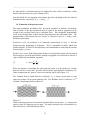
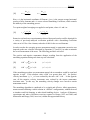
CROSS-SECTION SHAPE FACTOR: A factor that accounts for the shape of the
channel cross-section. It is defined as the ratio between the hydraulic (average)
depth and the maximum depth of the channel cross-section. For example, a
triangular channel has a factor of 0.5 and an elliptical channel has a ratio of 0.67,
as illustrated in Figure 4. A rectangular channel has a factor of 1. This factor
allows the user to input the geometry of the slide mass in terms of the maximum
channel depth. The factor must be greater than zero.
IMPORTANT NOTE: Only one constant depth factor can be used for the entire path.
Therefore, a depth factor of less than 1.0 should only be used for highly confined
paths, that remain confined for most of their length.
B
Dmax
B
H
Dmax × 0.67 = H
Figure 4: Illustration of how DAN-W uses the cross-section shape factor to convert the
maximum depth of a non-rectangular channel (Dmax) to the corresponding hydraulic
depth (H). B is the channel width.
15
______________________________________________________________DAN-W
ƒ
ƒ
ƒ
ƒ
ƒ
SET PROBLEM EXTENTS: The problem extents, described in Section C.1, are
defined by the coordinates of the bottom left and upper right corners of the
problem, as indicated by the graphic on this screen.
INITIAL VELOCITY (if any): A constant initial velocity in m/sec can be input
to be used in the next run. This variable is not stored in the problem file and is
reset to zero each time a new file is read, or whenever the Control Parameters
screen is re-open.
UNIFORM THICKNESS: Optional. Allows the user to enter a uniform
thickness (in metres) for the top surface geometry. If chosen, DAN-W will create
a top surface that will have the defined uniform thickness everywhere above the
slope. Note that this thickness is measured parallel to the type of slices used
(normal or vertical). Please refer to Section C.7 for further details.
CONFIGURATION: Allows the user to choose between the two-dimensional
configuration and the 3-dimensional configuration
END CONDITIONS: Allows the user to fix the front or the rear of the slide mass
in their initial position. A fixed end will not flow during analysis. This option is
useful in cases where the movement of an end point is restrained by the presence
of a wall (Figure 5).
Figure 5: Example where the left end condition is fixed and the right end is free.
The Continue item in the menu will accept all the input data and either return to the main
menu or continue to the next input screen in the New File Sequence. The Cancel option
will ignore any changes made in this screen and return to the main menu. Note that
choosing Cancel during the New File Sequence will cancel the new file completely.
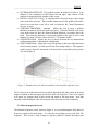
C.5 Material properties screen
The Material Properties screen, shown in Figure 6, is accessed through the Edit-Material
Properties option in the main menu. It is also the second input screen in the New File
Sequence. This screen is used to input or edit the problem’s material rheologies and
16
______________________________________________________________DAN-W
properties. It also allows the user to add and delete materials. The user has a choice of
eight rheologies, including:
ƒ
ƒ
ƒ
ƒ
ƒ
ƒ
ƒ
Frictional
Plastic
Newtonian
Turbulent
Bingham
Coulomb Frictional
Voellmy
These rheologies are described in Appendix 1, and in Hungr (1995). Each rheology
requires input of specific material properties, as listed in the first column of the table.
Properties that are not associated with a given rheology type are disabled (yellow letters).
The colour field above the columns indicates the colour of the line drawing the segment
occupied by the given material.
Figure 6: Material Properties screen.
The following is a list of all the material properties shown in this screen and a brief
description of each. For further explanation of the parameters see Appendix 1.
ƒ
ƒ
ƒ
MATERIAL: Optional. Any alphanumeric string representing the name of the
material.
UNIT WEIGHT: Unit weight of the material in kN/m3. Must be greater than 0.
SHEAR STRENGTH: Constant shear strength of the material, such as the
constant steady state undrained strength of a liquefied soil (plastic model).
17
______________________________________________________________DAN-W
ƒ
ƒ
ƒ
ƒ
ƒ
ƒ
ƒ
FRICTION ANGLE: Basal friction angle, in degrees (frictional model).
PORE-PRESSURE COEFFICIENT: Ratio of the pore pressure to the total
normal stress at the base of the sliding mass (frictional model).
VISCOSITY: Dynamic viscosity of the fluid (kPa .s) (viscous model).
FRICTION COEFFICIENT: First coefficient used in the Voellmy model. It is
equivalent to the tangent of the basal friction angle (dimensionless).
TURBULENCE COEFFICIENT: In the turbulent rheology: number that
represents the roughness coefficient in the Manning equation. In the Voellmy
rheology it is the coefficient that defines the turbulent term of the basal flow
resistance equation, which equals the square of the Chezy coefficient (m/s2).
EROSION DEPTH: Maximum depth to which the material is eroded after the
whole slide mass passes over it (in metres). A positive value indicates material
erosion.
INTERNAL FRICTION ANGLE: Angle that defines the internal friction acting
within the body of the flowing mass, as it stretches or contracts. This is used to
derive the tangential stress coefficients ka and kp (see Appendix 1). DAN-W
assumes that all materials are frictional when they deform internally. A zero
value should be used for fluids. NOTE: A default value of the internal friction
angle is set to 35°, which is appropriate for dry fragmented rock. The user should
experiment with other values, although generally, the model is not too strongly
sensitive to it.
Each material is assigned a colour, shown in the top row of the table. These colours are
used to draw the material segments in the isometric or profile view of the problem. To
add a material, place the cursor in the next available column in the table. To insert a
material in front of another material, place the cursor on the column where the new
material is to be inserted. Then select the Insert Material option from the menu. To
delete a material, place the cursor on the column to be deleted and select the Delete
Material option from the menu.
The Continue option in the menu will accept all the input data and either return to the
main menu or continue to the next input screen in the New File Sequence. The Cancel
option will ignore any changes made in this screen and return to the main menu. Note
that choosing Cancel during the New File Sequence will cancel the new file completely.
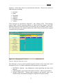
C.6
Material locations screen
The Material Locations screen, shown in Figure 7, is accessed through the Edit-Material
Locations option in the main menu, or as the final screen in the New File Sequence. This
screen allows the user to determine the location of each material segment along the length
of the slope profile. The coordinates of all the points input in the Edit Path screen are
shown on the left of the table. The user can set what material is located at which path
segment(s) by inputting the appropriate material’s code number in the MATERIAL
column. If no or the wrong material code is given, then DAN-W automatically assumes
18
______________________________________________________________DAN-W
the first material. The material properties of each element change when a new segment is
entered by it. Sometimes, two materials can be identical, but differ in erosion depth.
The Continue option in the menu will accept all the input data and return to the main
menu.
Figure 7: Material Locations screen.
C.7 Edit path/top screen
The Edit Path/Top screen, shown in Figure 8, is accessed through the Edit-Path or the
Edit-Top options in the main menu, or as the third screen in the New File Sequence. This
screen allows the user to input and edit the problem’s slope (path) and sliding mass (top)
profiles. The coordinate system used in this screen is described in Section B.3.
The data, prepared as described in Section C.1, can be input graphically by clicking the
mouse in the appropriate positions on the screen. Alternatively, data can be input
numerically in the provided table. Points can only be input from left to right, without
forming vertical steps or overhangs.
Points can be inserted between two existing points by selecting the Points-Insert Point
option from the menu and clicking either on the screen or in the table in the desired
position. Points can be deleted by selecting the Points-Delete Point option from the
menu and clicking the point to be deleted on the screen or in the table. All the points in
the selected line can be deleted by selecting the Points-Delete Line option from the menu.
19
______________________________________________________________DAN-W
The user can toggle between the path profile and the top profile on the menu. The current
profile being edited is drawn in red, while the other profile is drawn in blue. If the user
selected a uniform thickness top surface in the Control Parameters screen, then only the
first and last data points entered for the top surface will be read. These two points will
determine the front and the rear of the slide mass, while the slide mass in between these
points will follow the path profile at the uniform thickness specified. The thickness will
be measured according to the type of boundary block geometry chosen in the Options
screen (either normal or vertical). It is recommended that normal slices be used with the
uniform thickness option.
As the points are entered, the spline function, which DAN-W uses to smooth out the path
profile for analysis, appears as a purple line. The input points should be strategically
placed, so that the spline will approximate the actual path profile to the maximum extent.
In case of uneven paths, this may require insertion of additional points in some location.
The front and the rear of the slide mass (first and last points in the top profile) should
coincide with points on the path profile. To simplify this process, this screen has a builtin “snap” function that automatically snaps points together when they are close together.
IMPORTANT NOTE: The profile actually analysed by DAN-W is the spline profile,
shown by the purple line. The red lines on the input screen are merely straight line
connections between adjacent points.
Figure 8: Edit Path/Top screen. In this figure, the path is selected in red, while the spline
interpolation is drawn over it in purple. The top profile is drawn in blue.
As an alternative, the input points can be entered in the table on the upper right side of
the screen. Points can also be inserted or deleted directly in the table. To prevent
20
______________________________________________________________DAN-W
obstruction of screen graphics, the table can be dragged to any position on the screen. It
can also be made invisible by right-clicking the mouse.
A background bitmap image can be loaded and scaled to the screen coordinates to allow
the user to trace a pre-drawn cross-section. Loading and scaling an image is done by
choosing the Image-Load Image option in the menu. Once an image is loaded, the user is
asked to input the coordinates of two known points on the image. These two points must
be located on the bottom left and the top right of the picture, as shown in Figure 9. The
user is then asked to locate these two points on the image shown on the screen. Note that
the more precisely these points are located on the image, the better the image scaling will
correlate with the screen coordinate system. The image should then scale itself to the
screen. The image can be unloaded or rescaled by selecting the appropriate option under
the Image menu. The image will remain in the background of this screen as long as the
current file remains loaded in DAN-W or until the Unload option in the menu is chosen.
Sometimes the scaling may become distorted during editing operations. The best way to
correct this is to unload the image and re-load it again.
Figure 9: Example of a scanned image with known coordinates marked in blue at the
bottom left and upper right corners of the image.
The screen can be zoomed in or out to help with the graphical input of points. To zoom
in, select the View-Zoom In option in the menu and click the centre of the desired region.
To zoom in on a specific rectangular region, select the View-Zoom Box option then click
and drag across the region to be zoomed. Click the Zoom button in the bottom left of the
screen to zoom in on the red extents drawn on the screen. To zoom out, select the ViewZoom Out option in the menu. The View-Fit to Screen option will return the screen to its
original zoom position.
Pressing and holding the SHIFT key and the left mouse button together, allows the user
to drag the profile (including the background image) across the screen. This is useful
when tracing images at higher zoom levels.
21
______________________________________________________________DAN-W
The Continue option in the menu will accept all the path and top geometry data and will
return to the main menu or to the next screen in the New File Sequence. Alternatively,
the user can continue to the Edit Width Screen by choosing Edit-Edit Width from the
menu. In either case, the user will be warned if the path or top geometry has been input
incorrectly or is incomplete and will not be allowed to continue.
C.8 Edit width screen
The Edit Width screen, shown in Figure 10, is accessed through the Edit-Width option in
the main menu or as the fourth screen in the New File Sequence. This screen is used to
input or edit the channel width and is not accessible in the two-dimensional
configuration. The data should be prepared as described in Section C.1. This screen
functions like the Edit Path/Top screen (see previous section), except that the vertical axis
represents the channel width (in metres). The width of the problem should be completely
defined by the user between the two purple lines. NOTE: Initially, when a file is being
created, there is a default line defined by two points, with a uniform width of 1m (as in
2D configuration). These points can be dragged to correct locations and new points are
then added.
Figure 10: Edit Width screen.
C.9 Options screen
22
______________________________________________________________DAN-W
The Options screen, shown in Figure 11, is accessed through the Edit-Options or the
View-View Options selections in the main menu. This screen has three tabs, allowing the
user to edit various boundary, display, and analysis options.
Figure 11: Options screen.
The following is a list of all the options with a brief description of each:
Boundaries Tab:
The options under this tab are also accessible in the Control Parameters screen.
ƒ LEFT AND RIGHT BOUNDARIES: These options allow the user to fix the rear
(left) or front (right) of the slide mass during analysis. For further details, please
refer to Section C.4. Default = Free.
ƒ NUMBER OF ELEMENTS: This option allows the user to specify the number of
mass elements that the slide mass is to be split into. The recommended minimum
is 50.
ƒ TOP SURFACE INPUT: This option allows the user to choose the type of data
input used to define the top surface. The Manual option requires that the user
input data points through the Edit-Top screen. The Uniform Thickness option
allows the user to input a slide mass of uniform thickness above the path profile,
as described in Section C.4. Note that the thickness must be defined in the
Control Parameters screen otherwise it defaults to 1 metre. Default = Manual.
23
______________________________________________________________DAN-W
Display Tab:
ƒ
ƒ
ƒ
ƒ
ƒ
ƒ
ƒ
ƒ
PROJECTION ANGLE: This option allows the user to choose a projection angle
in degrees for the three-dimensional isometric plot displayed in the main screen.
This angle should be between 0 and 90 degrees. Default = 30.
ENLARGEMENT OF FLOW DEPTH: This option allows the user to input a
normal (or vertical) depth exaggeration ratio to help view the profile of very thin
landslides. A value of 1 means no exaggeration. Default = 1. Note that the
exaggeration ratio will also affect graphical output options. Large exaggeration
ratios may induce apparent irregularities of the flow surface in highly curved
paths. The depth exaggeration ratio has no effect on the analysis.
PLOTTING MODE: This option allows the user to choose the type of plot shown
in the main screen. If Isometry is chosen, an isometric view of the problem is
shown in the main screen and is defined by the projection angle described above.
If Depth Profile (2D) is chosen, the sliding mass’s velocity and thickness profiles
are plotted on the screen. These plotting modes are described in greater detail in
Section D.1. Default = Isometry.
VELOCITY EXTENTS: This option allows the user to specify the extents of the
vertical axis of the velocity graph displayed in the main screen when the plotting
mode is set to Depth Profile (2D). This option essentially allows the user to zoom
in or zoom out on the velocity profile. It is only available when the Depth Profile
option is chosen. Default = 0 - 50 m/s.
OBSERVATION POINT: This option allows the user to place an observation
point anywhere along the length of the path profile, as described in Section E.5.
Default = Off.
LOCATION ALONG X-AXIS: This option allows the user to specify the
location of the observation point along the x-axis. It is only available when the
Observation Point option is turned on. Default = 0.
ANIMATION SPEED: UPDATE GRAPHICS EVERY … SECONDS: This
option allows the user to specify how often the screen graphics are updated during
analysis. A larger number causes the graphics to be redrawn fewer times during
the run and hence increases the speed of the analysis. The animation, however,
becomes less smooth. Note that this option affects the screen graphics only.
Background analysis calculations still occur for every time step regardless of the
animation speed. Default = 0.02 sec.
LINES: This option allows using thick or thin lines in drawing the display.
Analysis Tab:
IMPORTANT NOTE: The following five parameters have an influence on the analysis
process. It is recommended that the default values be used for routine work.
ƒ
SMOOTHING COEFFICIENT: This coefficient controls the intensity of the
velocity smoothing process, as described in Appendix 1. It is recommended to
accept the default value of 0.02, to which the automatic time step evaluation is
24
______________________________________________________________DAN-W
ƒ
ƒ
ƒ
ƒ
ƒ
ƒ
ƒ
calibrated. Specifying the coefficient as zero will turn off the velocity smoothing
process.
TIP RATIO: This option allows the user to define the shape of the first and last
mass elements on the slide mass. A ratio of 0.5 represents triangular end
elements, while a ratio of 1 represents rectangular end elements. Default = 0.5.
STIFFNESS COEFFICIENT: This option allows the user to modify the stiffness
coefficient, which is described in Hungr (1995). Default = 0.05.
STIFFNESS RATIO: This option allows the user to modify the ratio between the
unloading and loading stiffness, which is described in Hungr (1995). Default = 5.
CENTRIFUGAL FORCES: This option allows the user to turn on or off the
centrifugal forces caused by the curvature of the slope profile. Default = On.
TRAJECTORY LAUNCH: This option turns on or off the option of the landslide
launching into ballistic trajectory, as described in Section D.4. Default=Off.
BOUNDARY BLOCK GEOMETRY: This option allows the user to choose
between boundary blocks created by vertical slices or slices that are normal to the
path. Vertical slices should be used if the rupture surface in the source area is
highly curved. If normal slices were to be used in this situation, the geometry of
the sliding mass would be distorted, as explained in Section C.2. Default =
Normal.
PRESSURE TERM: Recent research showed that the Savage-Hutter assumption
of lateral stresses between slices may be incorrect in some cases, particularly
those involving a large amount of lateral spreading (see Hungr, 2008, re-print
attached with program package). Releases 8 and higher default to the Modified
Savage-Hutter assumption, as described in the paper, which usually yields the
best results. Other alternative assumptions, also described in the paper and in
Section A.4 of Appendix 1, can be selected on the Edit/Options screen, but are not
recommended.
25
______________________________________________________________DAN-W
D ANALYSIS
26
______________________________________________________________DAN-W
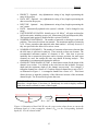
D.1 Graphics
Once all the data input is complete, two types of plots can be drawn in the main screen, as
listed under the View option in the main menu. The default plot shows an isometric view
of the slope and sliding mass profiles. An example is shown in Figure 12. This view
shows one half of the entire channel from the central cross-section out to the left margin
of the flow path. The grid lines on the screen relate to the central cross-section. The
projection angle and vertical exaggeration of the profile can be defined in the Options
screen. The sliding mass is drawn in black, while the slope profile is drawn in the
appropriate material segment colours, as defined in the Material Locations screen. The
boundary blocks within the sliding mass are shown in black when expanding, in red when
under compression, or in blue when in ballistic trajectory.
Central cross-section
Left margin
of path
Figure 12: Three-dimensional isometric view.
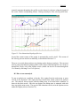
The second type of plot shows a two-dimensional depth profile of the sliding mass. It
consists of two graphs, one above the other, as shown in Figure 13. The upper graph
shows the current velocity profile of the sliding mass (drawn in black), as well as the
front velocity (drawn in blue) and rear velocity (drawn in purple) for each time step. The
lower plot shows the thickness profile of the sliding mass, including the current location
of all the boundary blocks (black normally and red if under compression). It also shows
the current erosion or deposition profile in the appropriate material colours. The various
27
______________________________________________________________DAN-W
material segments throughout the profile are also drawn for reference along the length of
the x-axis, in their corresponding colours. During an analysis, if the velocity profile runs
Current
Rear
Front
Erosion profile
Slide mass
Figure 13: Two-dimensional depth profile view.
beyond the current extents of the graph, it automatically rescales itself. The extents of
the velocity plot can also be set manually, as described in Section C.9.
The user can switch between these two plotting modes during an analysis. The run must
first be paused and then the plotting mode can be chosen either through the View menu or
through the Display tab in the Options screen (which can also be accessed through the
View menu by selecting View-View Options).
D.2 How to run an analysis
To run an analysis on a problem, select the Solve option from the main menu or press
Ctrl+R on the keyboard. This opens the Run Control Box which controls the analysis
run. The analysis always begins with the sliding mass in its initial static condition, as
drawn in the main screen. Once the run begins, the sliding mass is animated with each
time step in the main screen. The speed of the animation can be set in the Options screen
under the Display tab (see Section C.9).
28
______________________________________________________________DAN-W
D.3 Run control box
The Run Control Box, shown in Figure 14, is activated when the Solve option is selected
from the main menu. This box controls the analysis run of the problem. The time step
for the calculation is set automatically by the program, depending on the number of
elements and the length of the path. Although it is possible to change the time step value
in this window, the use of the default value is recommended for most analyses.
Figure 14: Run Control Box.
To begin the run, click the Run button or press Enter on the keyboard. The run can be
paused by pressing the Pause button. Pressing Run again will continue the analysis from
where it left off. Pressing Stop will finish and exit the run. Note that the plotting type (as
described in Section D.1) can be changed in the Pause mode.
As the problem is running, data calculated at each time step is displayed. The following
is a list of the displayed output along with a brief description of each:
ƒ
ƒ
ƒ
ƒ
ƒ
ƒ
ƒ
TIME: The total model time elapsed from the beginning of the run (seconds).
X-FRONT: The current position of the front of the sliding mass along the horizontal
axis (metres).
X-REAR: The current position of the rear of the sliding mass along the horizontal
axis (metres).
V-MIN: The velocity of the slowest boundary block in the slide mass at the current
time (m/s).
V-MAX: The velocity of the fastest boundary block in the slide mass at the current
time (m/s).
V-FRONT: The current velocity of the front of the sliding mass (m/s).
V-REAR: The current velocity of the rear of the sliding mass (m/s).
29
______________________________________________________________DAN-W
More detailed output can be accessed during the Pause mode by selecting the OutputReport option in the main menu. Please refer to Section E.1 for a description of this
screen.
When the run is stopped and exited, ASCII graph files are created if the user requested it
prior to the beginning of the run. Before completely exiting the run mode, the user is
given the chance to view the final Report for the problem as well as Observation Point
data if it exists.
D.4 Analysis options
1) Normal and Vertical Elements.
The DAN algorithm (Hungr, 1995) was originally created in terms of a depth-integrated
Lagrangian solution, referenced to columns normal to the path. This is still considered
the most reliable form of the solution, although the normal slice construction necessarily
distorts the geometry in case of deep and strongly curving paths (cf. example problem
SLUMP.DNW). The present version of the program also offers a solution formulated in
terms of vertical slices. The selection is made on the Edit/Options screen. The advantage
of vertical slices is that the geometry is not distorted on curved paths. Usually, there is
not a very strong difference between the results of the two forms in cases where only
gentle slopes are involved. On steeper slopes, the vertical mode may give somewhat
different results. While the normal mode is probably superior, the results of a vertical run
may need to be considered in some cases in the interest of conservatism.
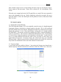
2) Trajectory flight.
A new feature has been added in Release 7, that makes the flowing mass launch into a
balistic trajectory when the normal stress on the base of the flow falls to zero. On screen
Figure 15. Trajectory flight
30
______________________________________________________________DAN-W
plots, a trajectory segment can be identified when the boundary elements appear in blue
colour (see Figure 15). While in trajectory, no base resistance acts on the slide,
regardless of the rheology. On landing, each element loses all of its momentum that is
normal to the path at that point.
Tangential (downslope) momentum parallel with the local base is conserved. It is to be
noted that this may be a conservative assumption in very strong (highly perpendicular)
impacts. Under such conditions, the trajectory model may lead to overestimation of
runout. When a strong impact occurs and the above method predicts a momentum loss of
more than 20% for this impact and for the leading element, the program pauses and a
dialog box appears, with the following information:
Large Impact:
Predicted loss of momentum amounts to 23%.
Enter estimated value of total momentum loss in %.
Press “OK” if you wish to retain the estimated percentage of momentum loss. Otherwise,
you can enter your own estimate of the energy loss (ranging from 0 to 100%). The
momentum loss you specify will be used for all “large” impacts from this point on.
“Small” impacts (momentum loss <20%) will still be treated in the standard way, as
specified at the beginning of this paragraph.
The trajectory option is turned OFF by default, but can be turned on in the
EDIT/OPTIONS/ANALYSIS. It is always off when vertical slices are used.
IMPORTANT WARNING: No verification benchmark tests involving the trajectory
option have so far been completed.
D.5 Model instability
The velocity smoothing algorithm is analogous to numerical damping used in many
numerical dynamic models to reduce instability. As such, it can have a certain effect on
the longitudinal spreading of the sliding mass. This influence could distort the results
under certain circumstances, when very small time interval is used. The program has
therefore been provided with a mechanism by which the time interval is set
automatically, to a value that has yielded reliable results in a range of benchmark cases.
The time interval is proportional to the number of elements. Therefore, smaller number
of elements will need less time. The number of elements usually does not influence the
runout results very strongly.
IMPORTANT NOTE: Do not use time intervals that are significantly smaller than the
interval set automatically by the program.
Solution instability may still occur in certain problems. It generally manifests itself by
series of translating waves, which rise in the rear of the slide mass and propagate to the
31
______________________________________________________________DAN-W
front. If such waves are observed, it is advisable to decrease the time interval from that
set automatically by a factor of 2 (but not more than a factor of 5).
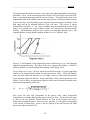
EXAMPLE: The example “SLUMP.DNW, enclosed with the program package,
illustrates the effects of instability. When run with normal slices (elements) and with the
automatically-set time interval of 0.0009 secs, the problem exhibits visible instability of
the flow front. The front horizontal runout position is 96.72 m and the final horizontal
coordinate of the center of gravity is 52.88 m. When the time interval is reduced to
0.0002 secs, the translatory waves disappear and the front stops at x=84.30 and the center
of gravity at 52.18 m. This result is considered to be superior in this case. The effect is
even stronger when vertical slices are used.
In general, it is recommended to reduce the time interval only where instability is clearly
apparent and only by the least amount necessary to remove the instability.
D.6 Verification testing
Releases 8 to 10 were checked against all of the verification benchmarks that were used
to verify the original model and published in Hungr (1995). New benchmarks,
specifically involving spreading flows are described in Hungr (2008). Comparisons
between DAN-W and DAN3D are described in Hungr and McDougall (2008). New
verification testing involving run-up against steep adverse slopes and accompanied by
shocks (representing run-up of flowing granular material against protective dykes) has
recently been completed (Mancarella and Hungr, in review, 2010, pre-print included with
the program package). The results indicate that DAN-W run-up predictions tend to be
conservative in case of runup against steep adverse slopes.
32
______________________________________________________________DAN-W
E DATA OUTPUT
33
______________________________________________________________DAN-W
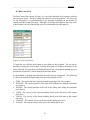
E.1 Report
The Report screen, shown in Figure 16, can be accessed by selecting the Output-Report
option in the main menu. This screen displays all the calculated values output during
problem analysis. The screen can be opened when a run is paused, as described in
Section D.3, or after the full completion of the run. The screen can also be printed by
selecting the Print button. The data displayed in this screen is described in the next
section. To export this data along with a list of materials and their properties into a text
file, select the Export button. This opens a screen where an appropriate folder can be
chosen to save the data in. Clicking Export in this screen creates a file called
OUTPUT.TXT. In this file, all numerical values are tab delimited from their
corresponding text descriptions. This allows the user to open the file in a spreadsheet
program.
Figure 16: Sample Report screen.
34
______________________________________________________________DAN-W
E.2 Output data
The following is a list of the output values displayed in the Report screen along with a
brief description of each:
ƒ
ƒ
ƒ
ƒ
ƒ
ƒ
ƒ
ƒ
ƒ
ƒ
ƒ
ƒ
ƒ
ƒ
ƒ
ƒ
ƒ
NUMBER OF ELEMENTS: The number of mass elements in the slide mass.
TIME STEP: The time step used during analysis (seconds).
END AT TIME: The total time elapsed since the beginning of the run (seconds).
CONFIGURATION: Two-dimensional or three-dimensional configuration.
SHAPE FACTOR: The cross-section shape factor used to define the shape of the
channel cross-section.
MAXIMUM VELOCITY: The maximum velocity reached by any boundary block
during the whole run (m/s), occurring at the given horizontal distance (metres).
MAXIMUM FRONT VELOCITY: The maximum velocity reached by the front of
the slide mass during the whole run (m/s), occurring at the given horizontal distance
(metres).
FRONT DISPLACEMENT:
ƒ HORIZONTAL LOCATION: The final location of the front of the slide mass
along the horizontal axis (metres).
ƒ CURVILINEAR DISPLACEMENT: The total displacement of the front of
the slide mass along the path profile (metres).
ƒ HORIZONTAL DISPLACEMENT: The total horizontal displacement of the
front of the slide mass (metres).
REAR DISPLACEMENT:
Same as for Front Displacement except for the rear of the slide mass.
CENTRE OF GRAVITY:
ƒ X-SOURCE / Z-SOURCE: The coordinates of the centre of gravity of the
initial, time zero position of the slide mass (metres).
ƒ X-DEPOSIT / Z-DEPOSIT: The coordinates of the centre of gravity of the
slide mass at the end of the run (metres).
CG RATIO: The ratio between the total vertical displacement of the centre of gravity
and the total horizontal displacement of the centre of gravity of the slide mass
(dimensionless).
TRAVEL ANGLE: The horizontal angle between the original centre of gravity and
the final centre of gravity (degrees).
FAHRBÖSCHUNG: The horizontal angle between the original rear of the sliding
mass and the final front of the sliding mass (degrees).
INITIAL / FINAL SLIDE VOLUME: The initial and final volumes of the slide mass
(m3).
INITIAL / FINAL AREA IN PLAN: The initial and final area in plan of the slide
mass (m2).
RUNOUT UNCOMPLETED, V-MAX: The problem was not allowed to settle. The
maximum velocity for the total run is displayed (m/s).
35
______________________________________________________________DAN-W
ƒ
RUNOUT TIME: The time it took the slide mass to completely settle (seconds).
E.3 How to create ASCII graph files
DAN-W can produce *.DAT data files in text (ASCII) format, which can be used to plot
profiles using GRAPHER (TM, Golden Software Inc.), EXCEL or any other graphing
software, including most spreadsheets programs. The types of profiles created and their
format are described in Section E.4.
To create ASCII graph files, select the Output-Export ASCII Graph Files option in the
main menu and then select the Create ASCII Graph Files option on the form that appears.
This enables the rest of the labels on the form, as shown in Figure 17. Choose a time
interval at which you want data to be collected for the profile plot and for the velocity
plot. It is recommended that the velocity plot have a smaller time interval than the profile
plot. Note, if you choose a time interval of zero, no files will be created. Next, choose a
folder in which to save the graph files in. Be careful not to choose a folder that already
contains other graph files of the same name, because they will be overwritten. Choose
OK to accept the information entered on the form. Now, to create the graph files, the
problem must be analyzed, as described in Section D.2. Once the run is stopped, a
message will be displayed notifying the user that the files have been created in the chosen
folder. Note that the vertical enlargement ratio, described in Section C.9, can be used to
make the data files more clear.
Figure 17: Export Graph Files screen.
36
______________________________________________________________DAN-W
E.4 ASCII graph file types
ASCII graph files containing profile data can be created by DAN-W, as described above.
The following is a list of the eight types of *.DAT graph files created. Note that the
column headings do not appear in the file, each column is tab delimited, and that the “a”
characters are read as empty cells.
ƒ
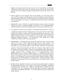
PR.DAT: Records at first the path profiles (original and modified by erosion or
deposition), then the slide mass profiles at the specified time intervals. An
example of the format of the file is shown below. A sample plot created from this
data file is shown in Figure 18.
X-Path
0.00
0.10
0.20
0.30
etc…
0.03
0.50
1.00
1.48
1.83
2.08
0.04
0.50
0.99
1.60
2.44
etc…
Y-Path
10.00
9.95
9.90
9.85
Width
2.00
2.00
2.00
2.00
X-Dep
0.00
0.10
0.20
0.29
Y-Dep
10.00
9.95
9.89
9.84
Y-Top1
Y-Top2
“a”
“a”
“a”
“a”
“a”
“a”
“a”
“a”
“a”
“a”
“a”
“a”
“a”
“a”
“a”
“a”
“a”
“a”
“a”
“a”
“a”
“a”
“a”
“a”
“a”
“a”
“a”
“a”
“a”
“a”
“a”
“a”
“a”
“a”
“a”
“a”
“a”
“a”
“a”
“a”
“a”
“a”
“a”
“a”
10.05
10.00
10.00
9.96
9.67
9.16
“a”
“a”
“a”
“a”
“a”
10.05
10.00
9.91
9.66
9.21
X-Path: X-coordinate of a point on the path.
Y-Path: Y-coordinate (elevation) of a point on the path.
Width: Path width.
X-Dep.: X-coordinate of a point on the path, modified by erosion or deposition.
Y-Dep.: Y-coordinate (elevation) of a point on the path, modified by erosion or
deposition.
Y-Top1: Y-coordinate of the top of each boundary block during the first profile
time interval.
Y-Top2: Y-coordinate of the top of each boundary block during the second profile
time interval.
37
2400
2400
2000
2000
1600
1600
1200
1200
800
800
400
400
0
1000
2000
Distance (m)
3000
Width (m)
Elevation (m)
______________________________________________________________DAN-W
4000
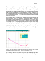
Figure 18: Sample profile plot created from PR.DAT, using GRAPHER (TM, Golden
Software Inc.). Black is the path profile; green is the top profile; orange is the erosion
profile; blue is the channel width; crosses indicate initial and final centres of gravity of
the slide mass, taken from CG.DAT.
ƒ
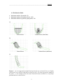
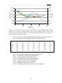
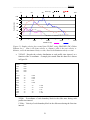
TR.DAT: Records velocities and positions of the front and rear of the mass, vs.
time. A sample plot created from this data file is shown in Figure 19.
Time
0.00
0.10
0.20
0.30
0.40
0.50
0.60
etc…
X-Rear
0.00
0.00
0.01
0.01
0.01
0.01
0.01
V-Rear
0.00
0.08
0.07
0.00
0.00
0.00
0.00
X-Front
2.00
2.04
2.14
2.32
2.55
2.85
3.18
V-Front
0.00
0.82
1.58
2.31
2.96
3.53
4.03
V-Max
0.00
0.82
1.58
2.31
2.96
3.53
4.03
V-Min
0.00
0.00
0.00
0.00
0.00
0.00
0.00
Time: Time in seconds, depending on the specified interval.
X-Rear: X coordinate of the rear of the sliding mass.
V-Rear: Velocity of the rear of the sliding mass.
X-Front: X coordinate of the front of the sliding mass.
V-Front: Velocity of the front of the sliding mass.
V-Max.: Maximum velocity at the current time.
V-Min.: Minimum velocity at the current time.
X-CG: X-coordinate of the centre of gravity of the flowing mass.
38
X-CG
1.16
1.18
1.22
1.28
1.37
1.49
1.63
______________________________________________________________DAN-W
Time (s)
0
20
40
60
80
100
100
Velocity (m/s)
80
60
40
20
0
-20
0
1000
2000
Distance (m)
3000
4000
Figure 19: Sample velocity plot created from TR.DAT, using GRAPHER (TM, Golden
Software Inc.). Blue is the front velocity vs. distance; pink is the rear velocity vs.
distance; red is the maximum velocity vs. time; black is the minimum velocity vs. time.
ƒ
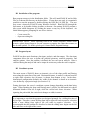
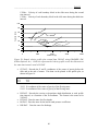
VE.DAT: Records the velocity distribution at each profile time interval, as a
function of the X-coordinate. A sample plot created from this data file is shown
in Figure 20.
X-Slide
-1.461
0.285
2.07
3.857
5.647
etc…
-1.455
0.291
2.075
3.863
5.652
etc…
0.823
2.507
4.317
6.144
7.983
etc…
V-Slide1
0.00
0.00
0.00
0.00
0.00
V-Slide2
“a”
“a”
“a”
“a”
“a”
0.346
0.334
0.332
0.33
0.328
”a”
“a”
“a”
“a”
”a”
“a”
“a”
“a”
“a”
“a”
V-Slide3
6.509
6.272
6.23
6.19
6.154
X-Slide: X-coordinate of each boundary block in the slide mass during each
profile time interval.
V-Slide1: Velocity of each boundary block in the slide mass during the first time
interval.
39
______________________________________________________________DAN-W
V-Slide2: Velocity of each boundary block in the slide mass during the second
time interval.
V-Slide3: Velocity of each boundary block in the slide mass during the third time
interval.
100
Velocity (m/s)
80
60
40
20
0
-20
0
1000
2000
Distance (m)
3000
4000
Figure 20: Sample velocity profile plot created from VE.DAT, using GRAPHER (TM,
Golden Software Inc.). Each line represents the velocity profile across the slide mass at
the same time intervals used in PR.DAT.
ƒ
CG.DAT: Records the X and Z coordinates of the centre of gravity before the
slide and at the end of runout. This data can be plotted in the profile plot, as
shown in Figure 16.
X-CG
11.53
64.72
Z-CG
52.39
17.82
X-CG: X-coordinate of the centre of gravity of the flowing mass.
Z-CG: Z-coordinate of the centre of gravity of the flowing mass.
ƒ
ƒ
ƒ
ƒ
DE.DAT: Records the erosion or deposition depth distribution at each profile
time interval, as a function of the X-coordinate. The format is the same as for
VE.DAT.
HT.DAT: Does the same for flow depths.
K0.DAT: Does the same for the lateral earth pressure coefficient.
DIS.DAT: Does the same for discharge.
40
______________________________________________________________DAN-W
E.5 Observation point
An Observation Point can be placed anywhere along the path profile to allow the user to
monitor the velocity and the thickness of the sliding mass at that point through time. To
set an Observation Point, choose the appropriate On option in the Options screen. The
location of the point can then be specified in the same screen. Once an Observation Point
is created, its location is shown in the isometric view by a short blue line on the front
cross-section, and in the depth profile by a vertical blue line extending down the screen.
Figure 21: Example of a plot created by DAN-W, showing the velocity and thickness of
the slide mass at a specified observation point location.
Figure 22: Export Observation Point screen.
41
______________________________________________________________DAN-W
After a run has been completed, the user can view a plot of the data collected, by
selecting the Output-Observation Point-View Data option in the main menu. An example
of the plot can be seen in Figure 21. The data can also be exported into a ASCII data file,
similar to those described in Section E.4. To export the data, choose the OutputObservation Point-Export Data option in the main menu. A form, shown in Figure 22,
appears in which the user can choose the appropriate folder to save the file in. When the
Export button is chosen, the data is saved in the chosen folder under the name OBS.DAT.
The first column in this file is time (in seconds) depending on the time interval chosen for
the analysis. The second column is the thickness of the slide mass (in metres) at this
location for each time interval. The third column is the velocity of the slide mass (in
metres per second) at this location for each time interval.
Note that with each subsequent analysis, all the previous Observation Point data stored by
DAN-W is replaced by the latest data.
42
______________________________________________________________DAN-W
APPENDIX 1
THEORY
43
______________________________________________________________DAN-W
The following paragraphs are a summary of the theory described in Hungr (1995 and
2008) and Mancarella and Hungr (2010).
The dynamic model DAN-W is based on the Lagrangian solution of St. Venant’s
equation. This equation can be derived by applying conservation of momentum to thin
slices of flowing mass that are perpendicular to the base of the flow. These “boundary
blocks” divide the slide mass into n “mass elements” of constant volume and are
separated by trapezoidal "mass blocks". If there is no entrainment, each of the mass
blocks carries a constant volume of (incompressible) material, so the equation of
continuity is implicitly satisfied.
1.1 Normal boundary elements
The original version of the numerical Lagrangian shallow flow model “DAN” (Dynamic
Analysis) was developed by Hungr (1995) and bears substantial similarity to the Savage-
Figure 1.1
Discretization of the Equation of Motion. n boundary blocks of infinitesimal thickness,
numbered i, are separated by (n-1) mass blocks, numbered j.
Hutter algorithm (Savage and Hutter, 1989). The equations are referenced to a moving
curvilinear coordinate system with s being the local downslope direction, h the bednormal thickness of the flowing sheet, α the slope angle, ρ density, t time, v mean
velocity and k the ratio between bed-normal and bed-parallel (longitudinal) stress within
the deforming sheet of material (see Figure 1.2a). Equation [1] is the momentum
equation applied to the boundary column:
44
______________________________________________________________DAN-W
a
b
Figure 1.2
Boundary column. a) bed-normal orientation, b) vertical orientation.
ρh
[1]
∂h
∂v
= ρhg sin α − kσ
−τ b
∂t
∂s
Given the shallow-flow assumption, the bed-normal stress, σ, acting on the base of the
flow equals:
σ = ρh( g cosα + ac )
[2]
Here, ac is the centripetal acceleration due to vertical curvature of the path, with a radius
R:
ac =
[3]
v2
R
In a frictional material without pore pressure, the resisting shear stress at the flow base,
τb, equals σ tanφb, where φb is the basal friction angle.
The coefficient k is the ratio between the bed-parallel and bed-normal stress and is
described in Section A.2.4.
1.2
Vertical element orientation
The vertical element orientation sometimes leads to distortion of the geometry at
locations where the path is strongly curved in the vertical plane. An alternative
formulation of the equations of motion uses elements that are mutually parallel and
vertical. In the vertical configuration, shown in Figure 1.2b, Equation [1] becomes:
45
______________________________________________________________DAN-W
[4]
ρh
dv
dh
= ρgh sin α cos α − ρh k cos α ( g + ac cos α ) − τ b
dt
ds
where h is now the flow depth, measured vertically.
Assuming that lateral (horizontal) unbalanced pressure acting on the vertical slice is
transmitted vectorially to the slice base, the bed-normal stress, σ, acting on the base of the
flow equals:
dh
k sin α ( g + ac cos α )
ds
The remaining equations and the manner of their discretization and explicit solution are
unchanged. The vertical framework produces similar results as the normal one.
However, the latter approach is probably somewhat more reliable, although it produces
more conservative results and apparently distorted plots where the path curvature is large.
The reason for this opinion is that the normal slice approach balances momentum and
impulse in the direction of motion.
[5]
σ = ρh cos α ( g cos α + ac ) + ρh
One consequence of the shallow-flow assumption is that shear stress acting on planes
parallel with the direction of integration, i.e. on the sides of the boundary blocks (Figure
1.2) is neglected. This simplification is inherent to all depth-integrated algorithms.
1.3 Method of discretization of the equations of motion.
The method of discretization of the equations was described in Hungr (1995, p.613)
Calculations are applied to a set of n “boundary” blocks and (n-1) “mass blocks”, each of
which carries a constant volume of material (Figure 1.1). The discretized variables that
apply to the boundary blocks include: bed-normal flow thicknesses, Hi, curvilinear
displacements, si and mean velocities, vi. Variables related to the mass blocks are block
volumes, Vj, flow thicknesses at mid-points of the blocks, hj and the pressure
coefficients, kj.
The analysis proceeds in an explicit manner, from the first block on the left. At each time
step, the velocity and displacement of each boundary block is determined by a numerical
integration of Equation [1] or [4]. This changes the curvilinear spacing of the boundary
blocks and the mass blocks compress, or stretch accordingly. The flow thickness at the
centre of each mass block is determined by Equation [6] (B is the local path width):
[6]
hj =
2V j
( si +1 − si )( Bi +1 + Bi )
The new thicknesses of the boundary blocks are determined as means of the adjacent
mid-point thicknesses from Equation [6]. Now, all the boundary block variables have
been updated and the analysis can proceed to the next time step. Longitudinal strain of
46
______________________________________________________________DAN-W
the mass blocks is calculated and used to update the value of the k-coefficient. Other
details of the procedure are given in Hungr (1995).
Note that DAN-W uses triangular end elements, therefore, the height of the first and last
boundary blocks, respectively, is h1 / 2 and hn-1 / 2.
1.4 Evaluation of the pressure term.
The usual assumption for shallow flow, developed originally for shallow, non-uniform
flow of fluids, is that the bed-normal stress is equal to the normal component of the
weight of the overlying fluid, plus a centrifugal force. The bed-parallel (longitudinal)
stress in the flowing mass is then assumed proportional to the bed-normal stress. The
proportionality ratio between the two stresses is referred to here as k, using a SoilMechanics convention.
Hydrostatic stress. In hydraulics, it is commonly assumed that k is one, i.e. that the
internal pressure distribution is hydrostatic. This is reasonable for fluids, which lack
internal strength. In DAN-W, the hydrostatic stress distrubution is used when the internal
friction angle, φi, is zero.
Rankine stress states. If the flowing mass behaves as a frictional material with an internal
friction angle φi and if the basal surface strength is negligible, the coefficient k can take a
value calculated by the Rankine equations:
[7]
π
φ
k = tan 2 ( ± i )
4 2
When an element is expanding, the major principal stress is in the normal (or vertical)
direction and the “active state” prevails, with the minus sign applicable in Equation [7].
Under compression, the "passive" state occurs and the sign is plus (Figure 1.3).
The “Rankine Passive Earth Pressure Coefficient”, kp, is always greater than 1.0 and
ranges up to about 5.0 for typical granular soils. The “Rankine Active Coefficient”, ka, is
less than 1.0 and ranges down to about 0.2.
Figure 1.3
General shearing trajectories associated with the Rankine stress states. a) compression
(passive) state, b) expansion (active) state. The major principal stress is horizontal in a)
and vertical in b). (After McDougall, 2006)
47
______________________________________________________________DAN-W
The distinction between the two states is set by the sign of the longitudinal strain (Savage
and Hutter, 1989). In the model proposed by Hungr (1995) and in the current DAN-W,
there is a gradual transition between the two stress states. The model keeps track of the
longitudinal strain in the sliding body and the earth pressure coefficients transit between
passive and active value depending on the strain developed in response to changes of the
path angle and on an assumed stiffness of the soil mass. The process is shown
schematically in Figure 1.4. The value of stiffness does not influence the results of the
model very strongly, but certain stiffness values are beneficial for improved model
stability. A dimensionless stiffness value of 0.05 is recommended (Hungr, 1995). The
rebound stiffness is larger than the loading stiffness, by a set "stiffness" ratio.
Figure 1.4 Development of the tangential pressure coefficient (ka or kp) with changing
cumulative tangential strain. The slopes of the curve represent the stiffness. In DAN, a
different stiffness is used on loading and unloading (after Hungr, 1995).
Savage-Hutter stress states. In cases where the basal friction angle, φb is more significant
relative to the internal friction angle, the principal stresses rotate. While the Rankine
states still exist within the material, it is no longer correct to assume that the principal
stress directions align with the bed. Savage and Hutter (1989) used the geometry of the
Mohr’s Circle to derive an approximate equation for the ratio between the normal stress
parallel and perpendicular to the bed:
[8]
1 ± 1 − cos 2 φ (1 + tan 2 φ ) 
i
b
 −1
k(min/ max) = 2 
2
φ
cos


i
Here again, the plus sign corresponds to the passive state, where bed-parallel
compression is occurring and the minus sign to the active state. The basal friction angle
φb may be the true dynamic friction between the base of the flowing mass and a
moderately smooth bed surface. However, more generally, it is the angle corresponding
to the current “friction slope”, given as the arc tangent of the ratio between the basal
shear stress and the normal stress.
48
______________________________________________________________DAN-W
"Modified" Savage-Hutter stress states. In case of spreading flows, where a very strong
positive depth gradient may exist, the flow lines become curved and a varying additional
clockwise shear stress is generated within the reference column by the unbalanced part of
bed-parallel pressure. As shown by Hungr (2008), the solution can be corrected by
replacing τb in Equation [8] with τb,mod so that:
tan φb ,mod = tan φb − λk (∂h
[9]
∂x
)
The modified shear stress is limited in calculations to positive values: tan φb ,mod ≥ 0 .
(Note: this parameter is not a basal stress and is not to be used in Equations [1] or [4].)
After testing various alternatives, it was found that the value of 0.333 for the coefficient λ
in Equation [9] produces the best results. The use of the Savage-Hutter relationship of
Equation [8], modified by reducing the basal friction angle as shown in Equation [9],
yields superior results in verification tests involving a variety of spreading flow
geometries, some of which diverge substantially from the shallow flow assumption. It
does not influence very strongly geometries that include shallow, elongated flow masses
such as is the case in avalanches.
1.5
The flow resistance term, τb
The basal flow resistance term, T, in eq. 1, is governed by the rheology of the material.
Eight rheologies are available in DAN-W. They are outlined below along with their
appropriate equations for T. A more detailed discussion can be found in Hungr (1995).
Plastic: Flow controlled by a constant shear strength c:
[10]
τb = c
Friction: Flow controlled by the effective normal stress on the base of the boundary
block:
[11]
where:
τ b = σ (1 − ru ) tan φ
ru = pore-pressure coefficient = ratio of pore pressure to total normal
stress at the base of a boundary block
φ = friction angle
NOTE: If ru is assumed to be constant, the resisting stress remains a linear function
of the normal stress and it is possible to replace the last term in Equation [11]
(1-ru)tanφ by the tangent of a constant "bulk friction angle" φb, where
tanφb = (1-ru)tanφ. This angle is the friction angle modified by pore-pressure and can
reach values much smaller than the dry friction of the basal material.
49
______________________________________________________________DAN-W
Newtonian flow: Viscous flow where τb is a linear function of velocity:
[12]
τb =
3vµ
h
µ = dynamic viscosity of fluid (kP.s)
where:
Turbulent flow: Flow where τb is a function of velocity squared:
[13]
τ b = γv 2 (
n
h
where:
1
)2
6
n = Manning roughness coefficient
Bingham flow: Flow where τb is a function of flow depth, velocity, constant yield
strength and Bingham viscosity:
[14]
where:
v=
c3
h
(2τ b − 3cb + b2 )
τb
6µ
µ = Bingham viscosity
cb = constant yield strength
Use of Equation [14] in the program requires the solution of a cubic equation at each time
step. Occasionally, the cubic solution may diverge.
Coulomb viscous flow: Bingham flow with a yield strength dependent on the normal
stress:
[15]
cb = σ (1 − ru ) tan φ
where the parameters are the same as for a friction flow
Voellmy fluid: Flow where τb contains a friction term and a turbulent term:
[16]
τ b = fσ + γ
v2
ξ
Here, the constant friction coefficient, f, is equivalent to tan(φb) in the frictional
model. The turbulence coefficient, ξ, is equivalent to the square of the Chezy constant
for turbulent water flow and v is the vertically-averaged velocity of the flow.
For further description of the alternative rheological relationships, please refer to Hungr
(1995 and 2008) and Hungr et al. (2005).
50
______________________________________________________________DAN-W
1.6
Material entrainment
The momentum flux term is based on how much material is deposited or entrained by the
slide mass. Working within the "supply limited erosion" framework, a total erosion
depth is specified within certain user-defined segments. As each mass element passes
over the path within this segment, a fraction of this depth (and hence, volume),
proportionate to the passing discharge, is eroded or deposited by the slide. The total
erosion depth is only removed once the entire slide mass has passed over the given point.
As the path material is entrained, the volume of the mass elements is increased by the
volume of material eroded. Path elevation change is neglected. At the same time, a
momentum correction is applied to the equation of motion, to account for the momentum
required to accelerate the added increment of stationary mass, ∆M, to the current velocity
∆M
of the boundary element, v. This is achieved by subtracting a quantity
v in each
∆t
time step of duration ∆t from the right hand side of Equation [1] or [4]. Note that this
momentum correction term would be zero for deposition of material (see Hungr, 1995,
page 616).
IMPORTANT NOTE: In normal operation, deposition of material is routinely neglected
(assuming that the full depth of the flowing mass will decelerate spontaneously). Thus,
the erosion depth is never specified as a negative number.
1.7
Velocity smoothing
A major problem with the earlier versions of DAN-W was that the model, which included
no damping, was not shock-capturing and tended to exhibit numerical instability when
applied to complex path geometries, particularly those that induce shocks on transition
between supercritical and subcritical flow. In order to prevent this, velocity smoothing
was introduced in Release 8, as described in the following.
It was observed that numerical problems usually arose when pairs of adjacent boundary
elements were forced close together, causing a rapid localized increase in depth in order
to maintain volume continuity. In order to mitigate this condition, weighted averaging of
the velocities of three adjacent boundary elements was introduced. The velocity of
Element i, vi was adjusted to a modified value vi’:
[17]
vi' =
vi −1 wl + vi + vi +1 wr
wl + 1 + wr
The weighting factors applied to velocities on the left and right of a given element, wl and
wr are scaled in inverse proportion to the horizontal gaps between the boundary elements:
51
______________________________________________________________DAN-W
[18]
wl =
∆xavg cs
xi − xi −1
wr =
∆xavg cs
xi +1 − xi
Here, xi is the horizontal coordinate of Element i, ∆xavg is the current average horizontal
spacing of all n elements and cs is a user-selected Smoothing Coefficient, which controls
the intensity of the smoothing process.
Two-point weighted averaging was applied to end points, where i=1 and i=n:
[19]
v1' =
v1 + v2 wr
1 + wr
vn' =
vn + vn−1 wl
1 + wl
Extensive trial-and-error experimentation showed that good results could be obtained for
a variety of previously-analysed verification problems with a Smoothing Coefficient
value set at 0.02 for a line element, reduced to 0.004 for the two end elements.
In order to make the averaging process momentum-neutral, a momentum correction was
imposed on the new velocities calculated by Equations [17] and [19], in order to maintain
the overall momentum of the mass. The following procedure was used:
The positive and negative momentum changes resulting from the application of the
smoothing equations during each time step was calculated:
[20]
∆M + = ρ ∑ (vi '−vi )hi
( vi ' − vi ) > 0
[21]
∆M − = ρ ∑ (vi '−vi )hi
( vi ' − v i ) < 0
If the smoothing procedure was momentum-neutral, the two numbers would be equal and
opposite in sign. If the absolute value of ∆M + was greater than ∆M − , the positive
velocity increments ( vi '− vi ) >0 were reduced by the ratio ∆M + / ∆M − . In the opposite
case, all the negative velocity increments were reduced by the inverse momentum
increment ratio. In this way, the smoothing velocity changes were forced to remain
momentum-neutral.
The smoothing algorithm is considered to be a simple and effective, albeit approximate,
means towards obtaining a stable solution in “difficult” configurations, without the need
to introduce artificial damping, or other shock-handling devices. Analyses of laboratory
experiments and other verification exercises reported in Hungr (1995 and 2008) and
Mancarella and Hungr (2010, in review) validate this approximate theory.
52
______________________________________________________________DAN-W
APPENDIX 2
REFERENCES
53
______________________________________________________________DAN-W
Ayotte, D. and Hungr, O., 2000. Calibration of a runout prediction model for debris
flows and avalanches. Procs., 2nd. International Conference on Debris Flows, Taipei,
Wieczorek, G.F. and Naeser, N.D., Eds., 505-514, Balkema, Rotterdam.
Ayotte, D., Evans, N. and Hungr, O., 1999. Runout analysis of debris flows and
avalanches in Hong Kong. Proceedings, Slope Stability and Landslides, Vancouver
Geotechnical Society Symposium May, 1999, 39-46.
Hungr, O. 1995. A model for the runout analysis of rapid flow slides, debris flows and
avalanches. Canadian Geotechnical Journal 32: 610-623.
Hungr, O., 2008. Simplified Models of Spreading Flow of Dry Granular Material.
Canadian Geotechnical Journal 45:1156-1168.
Hungr, O. and Evans, S.G., 1996. Rock avalanche runout prediction using a dynamic
model. Procs., 7th. International Symposium on Landslides, Trondheim, Norway, 1:233238.
Hungr, O., Dawson, R., Kent, A., Campbell, D. and Morgenstern, N.R., 2002. Rapid flow
slides of coal mine waste in British Columbia, Canada. In "Catastrophic Landslides"
Geological Society of America Reviews in Engineering Geology 15, pp. 191-208.
Hungr, O. and McDougall, S., 2009 Two numerical models for landslide dynamic
analysis. Computers & Geosciences Computers & Geosciences 35 : 978–992.
Mancarella, D. and Hungr, O., 2010. Analysis of run-up of granular avalanches against
steep, adverse slopes and protective barriers. Canadian Geotechnical Journal (in review)
McDougall, S. 2006. A New Continuum Dynamic Model for the Analysis of Extremely
Rapid Landslide Motion across Complex 3D Terrain. Ph.D. Thesis, Department of Earth
and Ocean Sciences, University of British Columbia (253 p.).
Revellino, P., Hungr, O., Guadagno, F.M. And Evans, S.G., 2002 Velocity and runout
prediction of destructive debris flows and debris avalanches in pyroclastic deposits,
Campania Region, Italy. Accepted by Environmental Geology, March, 2003.
Savage, S.B. & Hutter, K. 1989. The motion of a finite mass of granular material down a
rough incline. Journal of Fluid Mechanics 199: 177-215.
Tse, C.M., Chu, T., Wu, R., Hungr, O. and Li, F.H., 1999. A risk-based approach to
landslide hazard mitigation design. Procs., Hong Kong Institution of Engineers,
Geotechnical Division Annual Seminar, May 1999, 35-42.
54
______________________________________________________________DAN-W
APPENDIX 3
LIST OF WARNINGS AND ERROR MESSAGES
55
______________________________________________________________DAN-W
ARE YOU SURE YOU WANT TO DELETE ALL THE POINTS IN THE SELECTED
LINE?
All the points in the profile currently being edited will be permanently deleted.
ARE YOU SURE YOU WANT TO REVERT TO DEFAULT VALUES?
All values in the Options screen will be changed back to their default values.
CANNOT OPEN FILE ….
There is a formatting error in the file being opened.
CHOICE OF POINTS IS INCORRECT!
The first scale point must be located to the left and below the second scale point.
CROSS-SECTION SHAPE FACTOR MUST BE GREATER THAN 0.
The cross-section shape factor must be positive and non-zero.
FILE NOT FOUND. PLEASE TRY AGAIN.
The chosen image file is not found in the chosen directory. Check spelling or
check another directory.
FRICTION ANGLE OF MATERIAL # … MUST BE BETWEEN 0 AND 45
DEGREES.
Friction angle must be within the specified bounds.
FRICTION COEFFICIENT OF MATERIAL # … MUST BE BETWEEN 0 AND 1.
Friction coefficient must be within the specified bounds.
GEOMETRY ERROR. PLEASE CHECK GEOMETRY POINTS.
The solver encountered an error when setting up the problem geometry. Check
that all the data in the edit geometry screens corresponds to the rules described in
Section C.1, Section C.7, and Section C.8. Common reasons for the appearance
of this error are that the spline is very wavy or that all the top data points are
below the interpolated path data points.
GRAPH FILES: PATH … ACCESS ERROR.
The folder chosen to save the ASCII graph files in is read only. Please choose a
different folder.
IF YOU CHANGE TO A 2-DIMENSIONAL CONFIGURATION, YOU WILL LOSE
ALL OF YOUR WIDTH DATA. ARE YOU SURE YOU WANT TO CONTINUE?
Changing from a three-dimensional configuration to a two-dimensional
configuration will permanently replace all existing width data to unity.
LHS Y-COORDINATE MUST BE SMALLER THAN RHS Y-COORDINATE.
Problem extents must be defined by the lower left and the upper right coordinates
of the problem.
56
______________________________________________________________DAN-W
LHS Z-COORDINATE MUST BE SMALLER THAN RHS Z-COORDINATE.
Problem extents must be defined by the lower left and the upper right coordinates
of the problem.
MAXIMUM … ELEMENTS.
The number of mass elements must not exceed the specified amount.
MAXIMUM … MATERIALS ALLOWED.
The number of materials must not exceed the specified amount.
MUST HAVE AT LEAST ONE MASS ELEMENT.
The minimum number of mass elements is 1.
MUST HAVE AT LEAST ONE MATERIAL.
The minimum number of materials is 1.
NO OBSERVATION POINT DATA LOADED. YOU MUST RUN AN ANALYSIS
TO LOAD DATA.
Observation Point data is stored during an analysis and can be exported only after
the analysis is completed.
ONLY … POINTS ALLOWED.
Can’t add any more geometry points. The maximum has been reached.
PATH NOT FOUND. PLEASE TRY AGAIN.
The chosen path is incorrect. Try another directory.
PLOTTING ERROR. PLEASE CHECK GEOMETRY POINTS.
The solver encountered an error when plotting the three-dimensional problem
geometry. Check that all the data in the edit geometry screens corresponds to the
rules described in Section C.1, Section C.7, and Section C.8. Common reasons
for the appearance of this error are that the spline is very wavy or that all the top
data points are below the interpolated path data points.
POINT … MUST BE TO THE RIGHT OF POINT ….
Points in the edit geometry screens must go from left to right and must not
overlap.
PROJECTION ANGLE MUST BE BETWEEN -90 AND 90 DEGREES.
The projection angle for the isometric view in the main screen must be within the
specified bounds.
RUNOUT COMPLETE.
The slide mass has fully settled. The run is complete.
57
______________________________________________________________DAN-W
SLPINE ERROR. PLEASE CHECK GEOMETRY POINTS.
The solver encountered an error when spline-interpolating between the path data
points. Check that all the data in the edit geometry screens corresponds to the
rules described in Section C.1, Section C.7, and Section C.8. Common reasons
for the appearance of this error are that the spline is very wavy or that all the top
data points are below the interpolated path data points.
STIFFNESS COEFFICIENT MUST BE GREATER THAN 0.
The stiffness coefficient must be positive and non-zero.
THE PROBLEM HAS REACHED THE PROFILE EXTENTS. DO YOU WISH TO
CONTINUE?
The front of the sliding mass has reached the right-most extent of the slope
profile. Continuing beyond this point may result in instability.
THICKNESS MUST BE GREATER THAN 0.
The uniform thickness of the top above the path must be positive and non-zero.
TIP RATIO MUST NOT BE ZERO.
The tip ratio must be positive and non-zero.
UNIDENTIFIED ERROR # … OCCURRED: ….
An unidentified error, as described, has occurred when loading the image.
WARNING: POINTS … AND … HAVE EQUAL Y-COORDINATES AND WILL
MAKE THE SPLINE FUNCTION UNSTABLE. PLEASE MODIFY THE POINTS.
Path points with equal y-coordinates will cause the spline function to become
dramatically unstable. Make sure these coordinates are not the same and then test
the spline to make sure it gives the desired path profile.
WARNING, WIDTH ARRAY NOT DEFINED.
Must have at least two data points to completely define the channel width.
WEIGHT OF MATERIAL # … MUST BE GREATER THAN 0.
All materials must have a positive and non-zero unit weight.
WIDTH MUST BE GREATER THAN 0.
Must have at least two data points to completely define the channel width.
YOU MUST ENTER AT LEAST … POINTS IN ORDER TO PROPERLY DEFINE
THE … GEOMETRY.
Must have at least the minimum number of data points specified to completely
define the path, top, and width profiles.
ZOOM BOX EXTENTS ARE TOO SMALL
The chosen zoom box is too small. Please try again.
58