Download CHAPTER 4 RELIABILITY CONSTRAINTS The reliability constraints

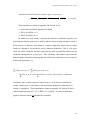
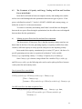
Long Term Model USER MANUAL, June 19, 2000
CHAPTER 4
RELIABILITY CONSTRAINTS
The reliability constraints insure that a proper reserve margin is maintained
between installed MW capacity and peak period MW demand in every period
PeakD(z)*dgr(z,ty).
Reliability requirements enter the model in two ways:
Requirement #1:
Each country must maintain a SAPP specified reserve margin for each of the
major sources of supply - thermal plants, including pumped storage, (Parameter RESTHM
in Appendix VI, Section 12 - default value 19%) and hydro plants (Parameter RESHYD 10% default value in Appendix V, Section 12). Since the model, as in the real world,
allows trade in reserves (imports held by others and exports held for others) to enter into
the equation, they must be added (Fmax(ty,zp,z), imports of reserves) and subtracted
(Fmax(ty,z,zp) exports of reserves) from the left hand side of the reserve equation.
Exports of reserves are simply subtracted, but imports of reserves need to be adjusted
downward by the line loss between z and zp; no adjustment for forced outage is
necessary, according to SAPP definitions of reserve requirements.
As in the case of the demand equation, a country can choose not to “meet” the
reserve constraint by choosing a positive value for unsatisfied reserve requirements –
variable UM(z,ty), and a cost/MW set by the user parameter UMcost found in Section 1
of Appendix II. (The nominal values set at $10,000/KW in the model.) This cost should
reflect the actual capacity cost of a backstop technology used in emergencies to generate
electricity, or, equivalently the actual cost of a demand side management program put in
place to shave peaks by load shedding during peak periods.
81
Long Term Model USER MANUAL, June 19, 2000
Available Installed Thermal Capacity
1+RESTHM (z )
+
Available Installed Hydro Capacity
1+RESHYD(z )
+ Reserves held by others to back up firm imports to"z" ( 1 - lineloss ) + UM ( z , ty )
− Re serves held by "z" to back up firm exports to others ≥ [ PeakD(z )*dgr (z ,ty ) − LM (z, th) ][ DLC (z ) ]
Note that the choice of RESTHM and RESHYD are behavioral choices; values can be
entered to reflect each SAPP member’s attitudes. The choice of FORICN and FORICO,
however, are set by the reliability of the lines connecting zp and z.
The full equation is as follows;
ty
PGOinit(z,i)(1 − DecayPGO ) n (ty ) + PGOexpstep(z,i)ÿ PGOexp (τ ,z ,i )(1 − DecayPGO ) n (ty −τ )
τ =1
+
ty
NTexpstep (z,ni)ÿ PGNTexp (τ ,z ,i )(1 − DecayNT ) n (ty −τ )
τ =1
ty
+ NSCexpstep (z,ni)ÿ PGNSCexp (τ ,z ,ni )(1 − DecayNSC ) n (ty −τ )
τ =1
+
ty
existing
thermal
capacity
PGNCCinit (z,ni)ÿ YCC (τ ,z ,ni )(1 − DecayNCC ) n (ty −τ )
τ =1
ty
+ NCCexpstep (z,ni)ÿ PGNCCexp (τ ,z ,ni )(1 − DecayNCC ) n (ty −τ )
τ =1
+
ty
PGNLCinit (z,ni)ÿ YLC (τ ,z ,ni )(1 − DecayNLC ) n (ty −τ )
τ =1
ty
+ NLCexpstep (z,ni)ÿ PGNLCexp (τ ,z ,ni )(1 − DecayNLC ) n (ty −τ )
ty =1
1 + RESTHM (z )
82
Long Term Model USER MANUAL, June 19, 2000
+
+
ty
HOinit (z,ih)(1 − DecayHO ) n (ty ) + HOV exp step (z,ih)ÿ HOV exp (τ ,z ,ih)(1 − DecayHO ) n (ty −τ )
τ =1
existing
hydro
capacity
+
ty
ty
HNinit (z,nh) ÿ Yh(τ ,z ,nh)(1 − DecayHN ) n (ty −τ ) + HN exp step (z,nh) ÿ HNV exp (τ ,z ,nh)(1 − DecayHN ) n (ty −τ )
τ =1
+
τ =1
PGPSOinit (z )(1-DecayPHO) n (ty ) + ÿ
phn
ty
ÿ [ PHNinit (z,phn)Yph(τ ,z ,phn)] (1 − DecayPHN )
τ =1
1+RESHYD (z )
reserves held in ty by
country zp for
country z , adjusted
for loss and
transmission forced
outage rates
+
ÿ ( Fmax(ty,zp,z ) ) (1 − PFOloss(zp,z ))
zp
+
unsatisfied reserve
requirements
peak demand in
year ty reserves in
ty held by country z
for use by country
zp
UM ( z , ty ) ≥
+ [ PeakD ( z ) dgr ( z,ty ) - LM ( z,th )] DLC ( z ) +
ÿ Fmax ( ty, z, zp )
zp
This reserve margin constraint, as stated in GAMS notation, is equation
ResvREG2 and is shown in Appendix VII, Section 14.
4.1
The Autonomy Constraint
In addition to system reliability considerations, non-technical, political, and
economic factors may require that domestic capacity be maintained at some prescribed
fraction of domestic peak demand, regardless of the economic advantages of importing
cheap power or reserve capacity. This will be the function of the country autonomy
constraint, which reflects the level of autonomy each country wishes to maintain, by
specifying a country autonomy factor, AF (z , ty ) ≥ 0 (found in Section 1 of Appendix
VI), which reflects each country’s desire to be completely self-sufficient ( AF ≥ 1),
willing to depend completely on firm imports during peak, if it is economic to do so
( AF = 0), or something in between; 0 < AF(z,ty) < 1 ;
83
n (ty −τ )
Long Term Model USER MANUAL, June 19, 2000
Available Installed Thermal plus hydro capacity in period ty ≥
≥ AF (z , ty ) D(peak ,y,z ) - DSM (peak ,y,z )
DLC (z )
∀ ty,z ,peak
These equations are found in Appendix VII, Section 16 for;
•
all but RSA and MOZ; Equation ResvREG4
•
RSA; ResvREG4 a, b, c
•
MOZ; ResvREG4 d, e, f
In addition to each country requiring that domestic production capacity (not
involving any reliance upon reserves held by others) always be large enough to satisfy a
given fraction of domestic peak demand, a country might also require that a certain
fraction of demand in all periods be met by domestic production. This is a far more
costly (to SAPP) constraint, because it prevents any trade (beyond that allowed by the
constraint) taking place in a given year. This constraint, when added would enter the
demand/supply constraint by requiring that x% of domestic production over a year be met
by domestic generation- e.g.
ÿ PG(ty, ts, td , th, z, i) + ÿ PGN (ty, ts, td , th, z, ni)
i
ni
+ÿ H (ty, ts, td , th, z , ih) + ÿ Hnew(ty, ts, td , th, z , nh) ≥ Enaf ( z, ty ) Demand
ih
nh
in all hours, days, seasons, and years, where Enaf(z,ty) is the fraction of demand in
country z during year ty which must be met by domestic production (Table Enaf(z,ty)
Section 1, Appendix I). These equations are found in Appendix VII, Section 26 and is
called “Equation Energy AF”, a, b, c (RSA), d, e, f (MOZ). It is only for illustrative
purposes, the base runs do not include this constraint.
84
Long Term Model USER MANUAL, June 19, 2000
4.2
The Treatment of Capacity and Energy Trading and Firm and Non-firm
Power in the Model
In an ideal world with no limits on computer memory and running time, models
such as ours would distinguish in the optimization between two types of power – Firm
power, as defined in section 2.17 Article 1 of SAPP’s ABOM, and economy energy, as
defined in section 2.11 of the same document.
To conserve on memory and running time Purdue’s model does not distinguish
between the two power flows during the optimization, but does allow users to distinguish
between them after the optimization.
A)
Splitting up power flows into firm and non-firm components
The characteristic of firm power flow is that the exporting country must have on
hand, either in the form of its own generating capacity, or capacity available from other
countries, sufficient capacity to always provide such power to the importing country.
In our model, this capacity commitment [or as section 2.27 puts it, “the lease of a
specific generating unit (or units) or a portion of such unit(s)”] is the variable
Fmax(ty,z,zp), representing country z’s “leasing” of capacity in ty to country zp.
Once Fmax(ty,z,zp) is known, along with the flow variables PF(ty,ts,td,th,z,zp)
and PFnew(ty,ts,td,th,z,zp), the following rules can be used to split up the flows between
z and zp into firm and economy trade;
Case A power flows exceed Fmax
If PF(ty,ts,td,th, z,zp)+ PFnew(ty,ts,td,th,z,zp)> Fmax(ty,z,zp);
Firm = Fmax(ty,z,zp)
economy = PF(ty,ts,tdt,th,z,zp)+ PFnew ( ty,ts,td,th,z,zp ) - Fmax(ty,z,zp)
Case B Power flows less than or equal to Fmax
If PF(ty,ts,td,th,z, zp)+ PFnew(ty,ts,td,th,z,zp)/
Fmax(ty,z,zp)
then;
Firm = PF(ty,ts,td,th,z,zp)+ PFnew(ty,ts,td,th,z,zp)
Economy = 0
85
Long Term Model USER MANUAL, June 19, 2000
Thus, all power flows are firm, unless power flows exceed the capacity commitment
represented by Fmax(ty,z,zp); only the excess (if any) of power flows over Fmax(ty,z,zp)
should be considered economy sales, since such sales are not backed up by any
committed capacity in the exporting country (e.g. “non-capacity, non-firm transactions” –
SAPP ABOM, service schedule “e”).
B)
Treatment in the Transmission Capacity Constraint
The flow variables for old and new lines - PF(ty,ts,td,th,z,zp) and
PFnew(ty,ts,td,th,z,zp) - power flows from country z to country zp in a given time slice –
give the total flow between two countries consisting of the sum of all firm and non-firm
power trades. Thus, the transmission capacity flow constraints for old lines involve only
PF(ty,ts,td,th,z,zp) and the current capacity of the old lines connecting z to zp – e.g., for
old lines (ignoring decay and forced outages);
ty
PF ( ty,ts,td,th,z, zp ) ≤ PFinit ( z,zp ) + ÿ PFOVexp ( tye, z,zp )
tye =1
a similar equation holds for new lines.
In addition, a constraint requiring that there be sufficient transmission capacity at
all times to handle the import/export of reserves must be added; e.g. the sum of current
new and old transmission capacity, derated by decay and forced outage, ≥ Fmax(ty,z,zp)
C)
Treatment in the Load Balance Constraints
The hourly load balances which require that supplies must equal demands,
involve only domestic generation, power imports, power exports, and demand. Ignoring
both unserved and dumped energy the load balance equation for the time slice (ty,ts,td,th)
is simply;
86
Long Term Model USER MANUAL, June 19, 2000
Sum of all Domestic Generation
+ ÿ PF(ty,ts,td,th, zp,z) ( 1- lineloss ) =
in (ty,ts,td,th)
zp
Demand in (ty,ts,td,th,z, zp)+ÿ PF(ty,ts,td,th,z,zp)
zp
No distinction is made between firm and non-firm power in meeting demand, nor should
there be; both can interchangeably satisfy the load balance equation.
D)
Treatment in the Reliability Constraints
According to section 2.33 and Appendix I of the SAPP ABOM, the reserve capacity
obligation of each country can be expressed as;
Thermal Capacity Hydro Capacity
+
≥ Peak Demand - Firm Power
1.19
1.10
Purchases + Firm Power Sales
Since firm power purchases/sales are not variables in the model, we use leased capacity
purchases/sales (Fmax(ty,z,zp)) in the equation, the purchases suitably adjusted for line loss and
outage rates;
Thermal Capacity in ty Hydro Capacity in ty
+
+ ÿ Fmax ( ty,zp,z )(1 − lineloss )
1.19
1.10
zp
≥ Peak Demand ( ty, z ) + ÿ Fmax ( ty,z, zp )
zp
To summarize:
•
Power flows between countries can after the fact be broken down into firm and
non-firm power;
•
Both the transmission and load balance constraints consider only the total flows of
firm and non-firm power.
87