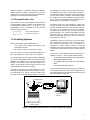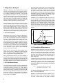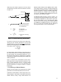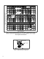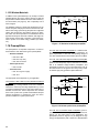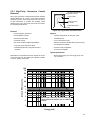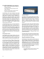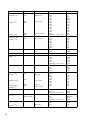
1
Nuclear Products Catalog Princeton Gamma-Tech, Inc. C/N 863 Princeton, NJ 08542-0863 USA Tel: (609) 924-7310 Toll Free: (800) 980-9284 Fax: (609) 924-1729 e-mail: [email protected] www.pgt.com © 1995,1998, 1999, 2000, 2002 Princeton Gamma-Tech, Inc. (formerly American Nuclear Systems, Inc.). All rights reserved. The following are trademarks or registered trademarks of Princeton Gamma-Tech, Inc: Quantum, Quantum MCA, Quantum-LIB, Quantum-X, QuantumGold. Printed in USA TRADEMARK ACKNOWLEDGMENTS The following are registered trademarks of the companies listed: Excel, Visual Basic; Microsoft, MS-DOS, and Windows, Microsoft Corporation; IBM, International Business Machines Corporation; Intel, Intel Corporation; GPIB, National Instruments. IMPORTANT!! PLEASE READ CAREFULLY NOTIFICATION OF COPYRIGHT THE FIRMWARE IN THIS DEVICE IS PROTECTED BY COPYRIGHT LAWS AND INTERNATIONAL TREATY. YOU MUST TREAT THE FIRMWARE LIKE ANY OTHER COPYRIGHTED MATERIAL. COPYRIGHT LAWS PROHIBIT MAKING ADDITIONAL COPIES OF THE FIRMWARE FOR ANY REASON OTHER THAN SPECIFICALLY DESCRIBED IN THE LICENSE BELOW. YOU MAY NOT COPY THE WRITTEN MATERIALS ACCOMPANYING THE PRODUCT. _____________________________________________________________ LIMITED WARRANTY / LIMITATION OF REMEDIES All hardware purchased from Princeton Gamma-Tech, Inc. (PGT) is covered by a one (1) year return to factory warranty. If your system was purchased directly from PGT, contact the factory directly. If the system was purchased from a distributor please contact your distributor prior to contacting the factory. A RMA number is required for returns and repairs. SUCH WARRANTIES ARE IN LIEU OF OTHER WARRANTIES, EXPRESS OR IMPLIED, INCLUDING, BUT NOT LIMITED TO, THE IMPLIED WARRANTIES OF MERCHANTABILITY AND FITNESS FOR A PARTICULAR PURPOSE WITH RESPECT TO THE SOFTWARE AND THE ACCOMPANYING WRITTEN MATERIALS. IN NO EVENT WILL PGT BE LIABLE TO YOU FOR DAMAGES, INCLUDING ANY LOSS OF PROFITS, LOST SAVINGS, OR OTHER INCIDENTAL OR CONSEQUENTIAL DAMAGES ARISING OUT OF YOUR USE OF OR INABILITY TO USE THE PROGRAM, EVEN IF PGT OR AN AUTHORIZED PGT REPRESENTATIVE HAS BEEN ADVISED OF THE POSSIBILITY OF SUCH DAMAGES. PGT WILL NOT BE LIABLE FOR ANY SUCH CLAIM BY ANY OTHER PARTY. This limited warranty gives you specific legal rights. Some states provide other rights, and states do not allow excluding or limiting implied warranties or limiting liability for incidental or consequential damages. As a result, the above limitations and/or exclusions may not apply to you. Furthermore, some jurisdictions have statutory consumer provisions which may supersede this section of the Agreement. GENERAL If any provision of this Agreement shall be unlawful, void, or for any reason unenforceable, then that provision shall be deemed severable from this Agreement and shall not affect the validity and enforceability of the remaining provisions of this Agreement. This Agreement is governed by the laws of the State of New Jersey. _____________________________________________________________ SERVICE AND SUPPORT You may contact PGT at any time for support issues. We can be reached by phone at (609) 924-7310, toll-free at (800) 980-9284 or by FAX at (609) 924-1729. We will be happy to discuss both technical and application problems with you. Contents About Princeton Gamma-Tech . . . . . . . . . . . . . . . . . . . . . . . . . . . . . . . . . . . . . . . . . . 1 Principles of Gamma ray and X-ray Radiation Detection . . . . . . . . . . . . . . . . . 3 1.1 Radioactivity . . . . . . . . . . . . . . . . . . . . . . . . . . . . . . . . . . . . . . . . . . . . . . . . . . . . . . 3 1.2 Photon/Matter Interactions . . . . . . . . . . . . . . . . . . . . . . . . . . . . . . . . . . . . . . . . . . . 3 1.2.1 The Photoelectric Effect . . . . . . . . . . . . . . . . . . . . . . . . . . . . . . . . . . . . . 4 1.2.2 Compton Scattering . . . . . . . . . . . . . . . . . . . . . . . . . . . . . . . . . . . . . . . . 4 1.2.3 Pair Production . . . . . . . . . . . . . . . . . . . . . . . . . . . . . . . . . . . . . . . . . . . . 4 1.3 Radiation Detection . . . . . . . . . . . . . . . . . . . . . . . . . . . . . . . . . . . . . . . . . . . . . . . . 5 1.3.1 Photon/Semiconductor Interactions . . . . . . . . . . . . . . . . . . . . . . . . . . . . 5 1.3.2 Fano Factor . . . . . . . . . . . . . . . . . . . . . . . . . . . . . . . . . . . . . . . . . . . . . . 6 1.3.3 Charge Detection . . . . . . . . . . . . . . . . . . . . . . . . . . . . . . . . . . . . . . . . . . 6 1.3.4 Preamplifier Rise Time . . . . . . . . . . . . . . . . . . . . . . . . . . . . . . . . . . . . . . 7 1.4 Counting Systems . . . . . . . . . . . . . . . . . . . . . . . . . . . . . . . . . . . . . . . . . . . . . . . . . 7 1.5 Spectrum Analysis . . . . . . . . . . . . . . . . . . . . . . . . . . . . . . . . . . . . . . . . . . . . . . . . . 8 1.5.1 Peak Location . . . . . . . . . . . . . . . . . . . . . . . . . . . . . . . . . . . . . . . . . . . . . 8 1.5.2 Peak Measurement . . . . . . . . . . . . . . . . . . . . . . . . . . . . . . . . . . . . . . . . 8 1.5.3 Quantitative Measurements . . . . . . . . . . . . . . . . . . . . . . . . . . . . . . . . . . 8 1.6 Timing and Coincidence Measurements . . . . . . . . . . . . . . . . . . . . . . . . . . . . . . . . 9 1.7 Detector Selection Parameters. . . . . . . . . . . . . . . . . . . . . . . . . . . . . . . . . . . . . . . 10 1.7.1 Detector Efficiency . . . . . . . . . . . . . . . . . . . . . . . . . . . . . . . . . . . . . . . . 10 1.7.1.1 Counting Efficiency . . . . . . . . . . . . . . . . . . . . . . . . . . . . . . . . 10 1.7.1.2 Absolute Efficiency . . . . . . . . . . . . . . . . . . . . . . . . . . . . . . . . 10 1.7.1.3 Relative Efficiency . . . . . . . . . . . . . . . . . . . . . . . . . . . . . . . . 10 1.7.1.4 Intrinsic Efficiency . . . . . . . . . . . . . . . . . . . . . . . . . . . . . . . . . 10 1.7.1.5 Efficiency of Marinelli Beakers . . . . . . . . . . . . . . . . . . . . . . . 11 1.7.1.6 Efficiency and Design of Well Detectors. . . . . . . . . . . . . . . . 13 1.7.2 Detector Resolution and Sensitivity . . . . . . . . . . . . . . . . . . . . . . . . . . . 14 1.8 Peak-to-Compton Ratio . . . . . . . . . . . . . . . . . . . . . . . . . . . . . . . . . . . . . . . . . . . . 14 1.9 System Noise and Microphonics . . . . . . . . . . . . . . . . . . . . . . . . . . . . . . . . . . . . . 14 1.10 Energy Range. . . . . . . . . . . . . . . . . . . . . . . . . . . . . . . . . . . . . . . . . . . . . . . . . . . 14 1.11 High Count Rates . . . . . . . . . . . . . . . . . . . . . . . . . . . . . . . . . . . . . . . . . . . . . . . . 14 1.12 Window and Endcap Materials . . . . . . . . . . . . . . . . . . . . . . . . . . . . . . . . . . . . . . 15 1.13 Low Background Spectroscopy . . . . . . . . . . . . . . . . . . . . . . . . . . . . . . . . . . . . . 15 1.14 Crystal Types and Geometries . . . . . . . . . . . . . . . . . . . . . . . . . . . . . . . . . . . . . . 19 1.15 Crystal Materials . . . . . . . . . . . . . . . . . . . . . . . . . . . . . . . . . . . . . . . . . . . . . . . . . 19 1.15.1 Crystal Shape . . . . . . . . . . . . . . . . . . . . . . . . . . . . . . . . . . . . . . . . . . . 19 1.15.2 Dead Layers . . . . . . . . . . . . . . . . . . . . . . . . . . . . . . . . . . . . . . . . . . . . 19 1.15.3 Window Materials . . . . . . . . . . . . . . . . . . . . . . . . . . . . . . . . . . . . . . . . 20 iii 1.16 Preamplifiers . . . . . . . . . . . . . . . . . . . . . . . . . . . . . . . . . . . . . . . . . . . . . . . . . . . 20 1.16.1 Preamplifier Characteristics. . . . . . . . . . . . . . . . . . . . . . . . . . . . . . . . 21 1.17 Maximum Count Rate Determination . . . . . . . . . . . . . . . . . . . . . . . . . . . . . . . . 22 1.18 High Count Rate Systems . . . . . . . . . . . . . . . . . . . . . . . . . . . . . . . . . . . . . . . . . 22 1.18.1 Noise Effects . . . . . . . . . . . . . . . . . . . . . . . . . . . . . . . . . . . . . . . . . . . 23 1.18.2 Gated Integrator with TR-14 Preamplifier . . . . . . . . . . . . . . . . . . . . . 24 1.19 Microphonics . . . . . . . . . . . . . . . . . . . . . . . . . . . . . . . . . . . . . . . . . . . . . . . . . . . 25 1.20 Pulse Processing Electronics and Software . . . . . . . . . . . . . . . . . . . . . . . . . . . 25 1.21 Cryostats . . . . . . . . . . . . . . . . . . . . . . . . . . . . . . . . . . . . . . . . . . . . . . . . . . . . . . 25 1.22 Detector Cool Down Requirements . . . . . . . . . . . . . . . . . . . . . . . . . . . . . . . . . . 27 PGT Products . . . . . . . . . . . . . . . . . . . . . . . . . . . . . . . . . . . . . . . . . . . . . . . . . . . . . . . . . . 28 2.1 Introduction . . . . . . . . . . . . . . . . . . . . . . . . . . . . . . . . . . . . . . . . . . . . . . . . . . . . . 28 2.2 Ordering Information . . . . . . . . . . . . . . . . . . . . . . . . . . . . . . . . . . . . . . . . . . . . . . 28 2.2.1 Sample Order . . . . . . . . . . . . . . . . . . . . . . . . . . . . . . . . . . . . . . . . . . . 28 2.3 Limited Liability Warranty . . . . . . . . . . . . . . . . . . . . . . . . . . . . . . . . . . . . . . . . . . 28 2.4 Selecting a Detector . . . . . . . . . . . . . . . . . . . . . . . . . . . . . . . . . . . . . . . . . . . . . . 29 2.5 Detector Specifications . . . . . . . . . . . . . . . . . . . . . . . . . . . . . . . . . . . . . . . . . . . . 2.5.1 Duo Detector . . . . . . . . . . . . . . . . . . . . . . . . . . . . . . . . . . . . . . . . . . . . 2.5.2 JT Cool Mechanically Cooled Spectrometer . . . . . . . . . . . . . . . . . . . . 2.5.3 High-Purity Germanium Coaxial Detectors . . . . . . . . . . . . . . . . . . . . . 2.5.4 N-type Coaxial HPGe Extended Range Detectors . . . . . . . . . . . . . . . 2.5.5 High-Purity Germanium Well Detectors. . . . . . . . . . . . . . . . . . . . . . . . 2.5.6 High-Purity Germanium Planar Detectors . . . . . . . . . . . . . . . . . . . . . . 2.5.7 N-Type HPGe Planar Detectors . . . . . . . . . . . . . . . . . . . . . . . . . . . . . 2.5.8 X-ray Detectors . . . . . . . . . . . . . . . . . . . . . . . . . . . . . . . . . . . . . . . . . . 2.5.9 Sahara Silicon Drift Detector . . . . . . . . . . . . . . . . . . . . . . . . . . . . . . . . 30 30 32 33 35 37 39 41 42 44 2.6 Endcap and Window Materials . . . . . . . . . . . . . . . . . . . . . . . . . . . . . . . . . . . . . . 46 2.7 Cryostats . . . . . . . . . . . . . . . . . . . . . . . . . . . . . . . . . . . . . . . . . . . . . . . . . . . . . . . 2.7.1 Dipstick Cryostats . . . . . . . . . . . . . . . . . . . . . . . . . . . . . . . . . . . . . . . . 2.7.2 Unitary Cryostats . . . . . . . . . . . . . . . . . . . . . . . . . . . . . . . . . . . . . . . . . 2.7.3 Portable Cryostats . . . . . . . . . . . . . . . . . . . . . . . . . . . . . . . . . . . . . . . . 2.7.4 Liquid Nitrogen Handling Devices . . . . . . . . . . . . . . . . . . . . . . . . . . . . 47 47 48 51 53 2.8 Mechanical Coolers . . . . . . . . . . . . . . . . . . . . . . . . . . . . . . . . . . . . . . . . . . . . . . . 55 2.8.1 JT Cool . . . . . . . . . . . . . . . . . . . . . . . . . . . . . . . . . . . . . . . . . . . . . . . . 55 2.9 Radiation Shields. . . . . . . . . . . . . . . . . . . . . . . . . . . . . . . . . . . . . . . . . . . . . . . . . 57 2.9.1 Model MPS-5 Radiation Shields . . . . . . . . . . . . . . . . . . . . . . . . . . . . . 59 2.10 Low-Background Materials . . . . . . . . . . . . . . . . . . . . . . . . . . . . . . . . . . . . . . . . 60 2.11 Electronic Components for Gamma-Spectroscopy with HPGe Detectors . . . . . . . . . . . . . . . . . . . . . . . . . . . . . . . . . . . . . . . . . . . . . . . . . . . . 61 2.11.1 Preamplifiers . . . . . . . . . . . . . . . . . . . . . . . . . . . . . . . . . . . . . . . . . . . 61 2.12 NaI(TI) Detectors . . . . . . . . . . . . . . . . . . . . . . . . . . . . . . . . . . . . . . . . . . . . . . . . 63 2.13 Quadratic Compression Conversion (QCC) — The New Way To Do NaI Gamma Spectroscopy . . . . . . . . . . . . . . . . . . . . . . . . . . . 2.13.1 MCA 2100R Multichannel Pulse Height Analyzer . . . . . . . . . . . . . . . 2.13.2 MCA 4000 Multichannel Analyzer . . . . . . . . . . . . . . . . . . . . . . . . . . . 2.13.3 System 4000 X-Ray Spectrometer . . . . . . . . . . . . . . . . . . . . . . . . . . iv 64 65 67 69 2.13.4 MCA 8000 Multichannel Analyzer . . . . . . . . . . . . . . . . . . . . . . . . . . . 72 2.13.5 System 8000 Gamma or X-Ray Spectrometer . . . . . . . . . . . . . . . . . . 74 2.13.6 Quantum MCA Software for Windows . . . . . . . . . . . . . . . . . . . . . . . . 77 Appendix 1: Radionuclides for Energy Resolution . . . . . . . . . . . . . . . . . . . . . . 81 Appendix 2: Radionuclides for Marinelli Beaker Standard Sources (MBSS) . . . . . . . . . . . . . . . . . . . . . . . . . . . . . . . . . . . . . . . . . . . . . . 82 Appendix 3: Major γ- and X-ray Lines for Various Radionuclides . . . . . . . . 83 Appendix 4: X-ray Critical Absorption and Emission Energies in keV . . . 87 Appendix 5: Glossary . . . . . . . . . . . . . . . . . . . . . . . . . . . . . . . . . . . . . . . . . . . . . . . . . . 89 v This page intentionally blank. vi About Princeton Gamma-Tech Princeton Gamma-Tech, founded in 1965, is an international supplier of high-performance gamma and X-ray spectroscopy products, including state-of-the-art, customized germanium detectors and systems. PGT merged with American Nuclear Systems (ANS) of Oak Ridge, Tennessee in 2000, and expanded the product line to include laboratory-based and portable sodium iodide (NaI) detectors and systems. High-purity germanium (also known as intrinsic germanium) became available in 1972-73. PGT produced the first commercial HPGe planar detectors that did not require lithium drifting, and could be stored at room temperature without performance degradation. PGT then produced the first HPGe coaxial detectors. These semiconductor radiation detectors were sold primarily to nuclear physics research laboratories. PGT continues to offer a wide selection of systems and components for many different types of measurements in environmental monitoring, health and safety, research, educational, and medical fields. PGT detectors have been used in a variety of locations including the bottom of a mine for double-beta decay studies of enriched germanium, in the ocean for remote sensing applications, and in a satellite for studies of the solar system. One high-profile use was in the Mars Observer. That detector included a cryostat with variable temperature control to permit in-flight annealing for repair of high energy photon and neutron damage. Its design requirements included the ability to withstand a stress of 50 G’s during launch. Even though the mission was ultimately aborted due to satellite failure, the detector functioned according to specification and returned valuable data on solar-flareinduced gamma-ray emissions. PGT also developed the QUIET ONE cryostat design technology, which allows the manufacture of mechanically cooled germanium detectors that still meet the stringent requirement for low microphonics. No other manufacturer offers this option. If your applications require mechanically cooled detectors with low microphonics design, ask for the JT Cool option. For gamma spectroscopy applications that require sodium iodide (NaI) technology, PGT has a complete line of systems and components to meet your needs. These include general-purpose multichannel analyzers with conversion gains from 1000 channels to 8000 channels and instruments specifically tailored to NaI detectors. This handbook is divided into several sections: •Section 1: Principles of Gamma ray and X-ray Radiation Detection (starting on page 3) provides detailed technical information about the basic principles of gamma and X-ray spectroscopy. •Section 2: PGT Products (starting on page 28) provides descriptions of and technical specifications for specific products. •The appendixes (starting on page 81) include useful reference materials and a glossary. If you require additional information or assistance, please contact the Nuclear Products Department. Our technical experts can help you assemble a new system, select a new detector, or repair and update an older detector purchased from another manufacturer. 1 This page intentionally blank. 2 Section 1: Principles of Gamma ray and Xray Radiation Detection Princeton Gamma-Tech specializes in the manufacture of semiconductor detectors for detection and high-resolution spectroscopy of gamma rays and X-rays. This section describes the basic principles of gamma ray and X-ray radiation detection. 1.1 Radioactivity ratio is unstable, and a stable configuration is achieved by emitting particle(s), gamma rays, or both. Radioactivity, or the rate of decay of such a radioisotope, is expressed as the number of disintegrations per second, or the rate of change of the number of nuclei (N) with time: dN ------- = – λN where λ = decay constant dT = 0.693/T0.5 Naturally occurring radioactivity—the emission of penetrating energy from matter—was first studied in depth in the late nineteenth and early part of the twentieth century. Max Planck deduced in 1900 that radiation is transmitted as discrete energy packets, which he called “photons.” Further work by scientists such as Rutherford, Curie, Einstein, Bohr, and others established the wave-particle duality of radiation, the interrelationship of matter and energy, and the basic understanding of atomic structure. Figure 1.1 is a simplified representation of the Bohr model of the atom, with a tightly packed nucleus of positively charged protons and uncharged neutrons and with negatively charged electrons in fixed orbits around the nucleus. γ ray (e.g., from 60Co decay) 1. K-shell electron is ejected by collision with a high energy particle or photon . . . . 2. . L-shell electron drops into the K shell 3. . . and a Kα X ray is emitted The decay constant is specific for each radioisotope and represents the probability of decay in the next second. The half life (T0.5) is the time required for half the current number of atoms (N0) to decay. The number of radioactive nuclides remaining after time t is then given by the equation: N = N e –λ t 0 Radiation may then react with matter to produce positively and negatively charged particles called ion-pairs. The three types of ionizing radiation are: • Photons (gamma rays and X-rays). • Charged particles (protons, electrons and alpha particles). • Neutrons (indirect ionizations). This discussion will concentrate on the interactions of photons (gamma rays and X-rays) in semiconductor detectors. The energy of a gamma ray or an X-ray is characteristic of its source. Gamma rays originate within the nucleus as a result of nuclear transformations and disintegrations, and have energies ranging from approximately 100 eV to 100 MeV. X-rays are the result of electron transitions from a higher-energy to a lower-energy electron shell of an atom, and have energies ranging from a few eV to almost 150 keV. The basic energy unit for this application is the electron volt (eV), equal to 1.6 × 10⁻¹⁹Joule. Figure 1.1 Schematic representation of gamma and X-ray generation with a Bohr model of the atom. The atomic number Z, the number of protons in the nucleus, determines the element. The mass number A is the total number of protons and neutrons in the nucleus. Protons and neutrons have nearly the same mass, and contribute almost the entire mass of an atom. Atoms having the same atomic number but a different mass number are called isotopes. In radioisotopes, the proton/neutron 1.2 Photon/Matter Interactions The three primary processes in which photons interact with matter to give up all or part of their energy in single events are: • The photoelectric effect (Section 1.2.1). • Compton scattering (Section 1.2.2). • Pair production (Section 1.2.3). 3 For a narrow beam of N0 photons traversing an absorber material of thickness y, the attenuation of the beam is given by the equation: N = N e – µy y 0 Compton effect: E’ E θ E′ where Ny = the number of remaining photons, and T CE E = ------------------------------------------------1 + E ( 1 – cos θ ) ⁄ 511 E = -------------------------1 + 511 ⁄ 2 E µ = the total attenuation coefficient for the three processes. 1.2.1 The Photoelectric Effect In a photoelectric event, the entire photon energy is absorbed by a bound atomic electron which is ejected with a kinetic energy equal to the photon energy minus the binding energy of the electron. The cross-section for the process increases with atomic number (~Z4 to Z5) and decreases rapidly with increasing photon energy (~E-3). The residual ion may return to its ground state by emitting one or more X-rays or an Auger electron. The low-energy X- ray is almost invariably absorbed in a second photoelectric event before it can escape from the crystal. As a result, the total photon energy appears as electron kinetic energy. Thus, a monoenergetic photon gives rise to a monoenergetic peak in the charge distribution corresponding to the incident photon energy. 1.2.2 Compton Scattering In the Compton Scattering process (shown in Figure 1.2) the photon is scattered by an electron with a partial energy loss which is dependent on the angle of scattering. The kinetic energy imparted to the electron is between zero and a higher value related to the energy of the photon. If the scattered photon escapes before further interaction, the detector will record only a fraction of the incident photon energy. These fractional photon energies appear in the spectrum at less than the full energy peak. As a result, the spectrum exhibits a continuous electron energy distribution, the Compton continuum, below the full energy peak of the incident photon. The cross-section for this process is proportional to the atomic number of the scattering material and is somewhat less energy-dependent than the photoelectric effect. The maximum energy in the Compton continuum is called the Compton Edge (CE). Events in which the CE energy is exceeded are normally photoelectric events. 1.2.3 Pair Production In pair production, an incident photon in the field of the nucleus of an absorber atom gives up all its energy to produce an electron-positron pair. Unlike the photoelectric effect and Compton scattering, which are possible at all energies, pair production has an energetic threshold equal to the combined positron-electron rest mass (1.022 MeV). Above this threshold, the cross-section for the event 4 E = energy of incident photon (keV) E’ = energy of scattered photon (keV) T= kinetic energy of the scattered electron θ = scattering angle CE = Compton edge, T when θ = 180° Figure 1.2 Compton scattering. increases rapidly with Z2 of the absorbing material up to about 10 MeV, beyond which it decreases because of screening effects. The entire photon energy (E) is converted to the kinetic energy of the positron-electron pair (i.e., E - 1.022 MeV) plus the rest mass of the pair. The positron is annihilated by an atomic electron, producing two 0.511 MeV photons emitted at 180° to each other. None, one, or both of these photons may escape, resulting in a spectral distribution that includes a full energy peak (FEP), a single escape peak (SEP), and a double escape peak (DEP) as shown in Figure 1.3. 104 FEP (E0) 180° scatter from inactive material 103 DEP θ = 180° Counts SEP 102 crystals with p-type impurities are counter-doped with ntype lithium ions. Ge(Li) detectors are no longer manufactured, but some are still in use. These crystals are fabricated into p-i-n diodes capable of withstanding high reverse-bias voltage with low current (<0.1 nAmp) at cryogenic temperatures. Figure 1.4 is a simple diagram of a detector. When the reverse bias is applied, the intrinsic region (i) is created by depletion of charge carriers. The detector crystal has a lithium-diffused N+ layer about 0.5 mm thick on one surface and a thinner P+ layer, formed by boron ion implantation or metallization, on the other surface. + V applied high voltage θ < 90 ° from Va θ > 90° from Vi 0 W θ > 90° from Va θ < 90° from Vi 500 E (keV) N+ layer 1000 θ = Compton scattering angle FEP = full energy peak SEP = single escape peak = FEP - 511 keV DEP = double escape peak = FEP - 1022 keV Va = active volume Vi = inactive volume Figure 1.3 Spectral distribution of a monoenergetic 1.4 Mev gamma ray incident on coaxial germanium. 1.3 Radiation Detection Radiation detectors measure the effects of incident particles or photons on matter. There are three main types of detectors: incident photon i -+ - P+ layer + - + W = crystal depth i = intrinsic region Er = electric field Er Figure 1.4 Schematic of photon/semiconductor interaction. In this type of semiconductor radiation detector, a photon interacts within the depletion region to release electrons and holes which move to the contacts of opposite polarity along the lines of the electric field (Er) established by the applied high voltage. The resulting charge is integrated by a charge-sensitive preamplifier to produce a voltage pulse with height (amplitude) proportional to the incident photon energy. 1.3.1 Photon/Semiconductor Interactions • Gas filled detectors • Ionization chambers • Proportional counters • Geiger-Müller counters • Scintillation detectors • NaI(Tl) and CsI(Tl) crystals Not all pulses produced by a mono-energetic photon source will have the same amplitude. Line broadening occurs due to statistical fluctuations and electronic noise. Also, some of the electron-hole pairs are trapped and do not reach the detector contacts, thus producing smaller signals which cause “tailing” on the low energy side of the peak. • Various plastics • Semiconductor detectors • High-purity germanium (HPGe) • Lithium-drifted silicon (Si(Li)) • Lithium-drifted germanium (Ge(Li)) PGT specializes in the manufacture of high-purity germanium (HPGe) and Si(Li) detectors for gamma and X-ray detection. HPGe crystals contain a non-zero level of impurities. The type of impurity determines whether the crystal is a p- or n-type semiconductor. For Si(Li) detectors, silicon Additionally, many of the interacting gamma rays are not completely absorbed in the detector, but are inelastically scattered and escape. This type of interaction yields a low energy Compton background. Finally, some photons reach the detector only after having been scattered by some material surrounding the detector or by the “dead” layer in the detector itself. These rays will also yield lower energy pulses. The relative importance of the photoelectric effect, Compton scattering, and pair production in germanium and silicon with respect to energy of the incident photon is illustrated in Figure 1.5. 5 uncorrelated partitioning of the energy between covalent bond-breaking and lattice vibrations or phonon production. Several competing mechanisms are involved in the energy loss. The Fano Factor (F) has been introduced to account for the variance in the number of electron-hole pairs produced. 10 PE = photoelectric effect C = Compton scattering PP = pair production Linear absorption coefficients (cm4) PE 1 If there were no variation in the number of electron-hole pairs, F would be 0. If there were a Poisson distribution of energy loss mechanisms, F would be 1. The actual value is closer to 0 than to 1. In most cases, a value of 0.11 for both silicon and germanium gives satisfactory agreement with laboratory results. C 10-1 PP 10-2 1.3.3 Charge Detection Germanium Silicon 10-3 10-2 10-1 1 Energy (MeV) 10 102 When a semiconductor detector is used in a spectrometer, the current signal from the detector is converted by a charge-sensitive preamplifier to a voltage signal, which is then processed in the main amplifier and multichannel analyzer (MCA). Figure 1.5 Linear absorption coefficients for Ge and Si as a function of gamma ray energy. In all these absorption processes, one or more energetic electrons result, and these in turn lose their energy largely through Coulomb interactions along the path of the electron in the absorber material. The principal effect of gamma ray interaction with semiconductors is thus ionization, which is shown by the creation of a large number of electron-hole pairs, in direct proportion to the energy of the incident photon. The average energy ε necessary to create such an electron-hole pair is: • 3.0 eV in germanium. • 3.76 eV in silicon at 77 K. • 3.6 eV in silicon at room temperature. These values are independent of the type or energy of the incident radiation. The relatively high atomic number, the low values of ε compared with the energy necessary to create an electronion pair in a gas, and the fact that they are independent of the type and energy of incident radiation make semiconductor detectors ideal for nuclear spectroscopy. 1.3.2 Fano Factor Comparison of these values with the forbidden bandgap values of 1.115 eV for Si at room temperature and 0.73 eV for Ge at 80 K provides evidence that not all the energy of the ionizing radiation is used in breaking covalent bonds. Some is converted to phonons in the lattice. The number of electron-hole pairs (n) produced at a given energy of incident radiation is not fixed, as would be the case if all the energy were used in breaking covalent bonds. Nor is there a Poisson distribution to indicate an 6 Z I(t) CD RD I(t) = current generator (in the detector crystal) CD = capacitance in the depletion region RD = resistance of the depletion region Z = series impedance Figure 1.6 Detector equivalent circuit. Determination of the current induced in the detector, as shown in the equivalent circuit in Figure 1.6, requires first calculating the motions of the charge carriers in the electric field, Er (see Figure 1.4). Er is readily calculated from the applied bias voltage, detector geometry, and bulk resistivity of the crystal. Once Er is known, the following differential equation can be solved: dr ----- = V ( E ) d r dt r = position of the charge carrier Vd = drift velocity in the electric field Er For the example shown in Figure 1.4, of a detector with plane parallel contacts and a field Ex across a distance W, the carrier q moving a distance x in the direction of the field induces a charge given by the following equation: ∆q ∆x = q ----W These two equations, or equivalent equations for different detector geometries, yield the contribution to I(t) of every charge carrier. The total induced charge I(t) is obtained by integration over all the charge carriers created. 1.3.4 Preamplifier Rise Time The rise time (Tt) of the generated pulse can be measured at the preamplifier output. For gamma and X-ray detectors, if the preamp is sufficiently fast, Tt is equal to TR, the charge collection time. An estimate of TR can be made from the following equations: ≅ W × 10 – 7 s T R ≅ W × 10 – 8 s TR for Si at room temperature for Ge at LN2 temperature 1.4 Counting Systems Nuclear spectroscopy requires determination of: • The energy of each voltage pulse induced in the semiconductor detector. • The number of pulses occuring at each energy. This is the function of the main amplifier/ADC/MCA system. In its simplest form, the process occurs as follows: corresponding to the given energy is incremented by one. The familiar spectrum display is essentially a histogram of the probability density of energies of the detected radiation, or a plot of the number of counts in each channel against the energy in the channel. In addition to counting and storing the data, the MCA provides the mechanisms for displaying, printing, and analyzing the information. The pulses arrive at the main amplifier at random time intervals. At higher count rates, the system is unable to discriminate between pulses if the time between events is less than 1.5× the peaking time of the main amplifier. The pulses pile up and cannot be processed, resulting in peak broadening. This spectrum degradation becomes significant when the product of input count rate and pulse processing time exceeds 0.5, and it is a dominant factor when this value is >1. Decreasing the pulse processing time of the main amplifier by decreasing the peaking time reduces the spectrum distortion, but produces a loss in resolution. To compensate, a pileup rejection module is frequently included in the circuitry and the ADC live time is extended to account for the time that the system is unable to process pulses. A typical PGT nuclear detector system is illustrated schematically in Figure 1.7. The components shown include: • A germanium detector with an external preamplifier and standard dip-stick cryostat. The voltage pulse from the charge-sensitive preamplifier goes to the main amplifier where it is shaped and further amplified. The shaping time is the time required by the amplifier to completely process each pulse. Several integrations are performed to smooth away most of the noise while retaining the information in the pulse. • An amplifier and ADC module such as the System 8000. The height of the pulse from the main amplifier is then converted by the analog-to-digital converter (ADC) to a number proportional to its energy. When this digital value arrives at the multi-channel analyzer (MCA), the channel The ADC and the main amplifier with pile-up rejection can be incorporated within the multichannel analyzer so that the output signal from the preamplifier is fed directly to the PC for processing and analysis. • A PC with spectroscopy software. Incident photon Preamp System 8000 PC with spectroscopy software Ge detector/external preamp & standard dewar Figure 1.7 Schematic representation of a nuclear spectroscopy system. 7 Detection of photons is only the first step of the analysis process. The spectral peaks must be located (see Section 1.5.1), their energies measured and identified with the correct nuclides or elements (see Section 1.5.2), and their areas quantified (see Section 1.5.3). These functions are done by computer analysis, and require certain preliminary calibrations for channel number vs. energy, detector resolution (peak width), and detector efficiency. A detailed discussion of spectrum analysis can be found in the users manuals for specific spectroscopy software products. A spectrum peak is a span of channels with photon counts that are statistically higher than those of the underlying continuum. A peak has a centroid with the highest counts, and a roughly Gaussian shape. The more channels per spectrum, the smaller the energy range per channel, but also the fewer counts per channel. Using too many channels may produce a broad, poorly defined peak. Commonly used spectrum sizes are 4096, 8192, or 16,384 channels . 1.5.1 Peak Location Peak location can be done by looking for differences in successive channels that define a more-or-less Gaussian shape. With a poorly defined, low peak on a background, this may be difficult to identify. More commonly, first or second order or higher derivatives of the spectrum curves are used. Since the spectrum is actually a histogram, the curve is approximated from the gradient of adjacent channels. The curve is smoothed by taking into account several channels at a time to eliminate some of the statistical scatter. The first derivative of the resulting curve changes sign at the centroid of a peak, while the second derivative shows a minimum at the centroid. Peaks may also be located by cross-correlation with a search function, such as a derivative of a Gaussian distribution. The spectrum data is digitally filtered to define a point in the peak with the background eliminated. After a potential peak has been found, its acceptability is determined by applying a threshold parameter to eliminate spurious peaks, while ensuring that small real peaks are recognized. The analytical software uses some multiple of the standard deviation to give the desired confidence level. 1.5.2 Peak Measurement Once a peak has been located, its energy is established by correlating its centroid with the channel energy. To do this, a calibration spectrum is obtained. For nuclear applications, the source consists of nuclides which produce singlet peaks of known energy. Usually two such points are sufficient, since energy calibration is nearly linear over most of the spectrum range. For X-ray applications, the calibration source may be element samples which yield X-rays of known energy when irradiated. 8 The energy of the located peaks is then matched with the known energies of gamma and X-rays in a nuclide or element library. In most cases, multiple peaks are produced by a given nuclide or element, and it is this set of peaks and their relative intensities that pinpoint an identification. Overlapping peaks may complicate the analysis, and in such cases peak stripping or deconvolution must be performed before the identification can be made. In addition to the generalized searches that locate, measure and identify all peaks as specific nuclides, librarydirected searches can also be done. Peaks of the nuclides or elements of interest are specified and the spectrum is searched in only the selected regions of interest (ROIs). Although this type of search is faster than a generalized search, it is more likely to miss an unexpected peak. Select a search type based on the requirements of the specific analysis. P = Full peak count Counts 1.5 Spectrum Analysis FWHM P = Half peak count 2 Background Channels or energy Figure 1.8 Determination of peak area. 1.5.3 Quantitative Measurements Quantitative analysis determines the area of a peak (peak integral in counts) attributable to the nuclide in question. In Figure 1.8, the background under the peak is assumed to be linear, as shown by the shaded trapezoid. The left and right sides of the peak are commonly defined by the full width half maximum (FWHM) of the full peak height (or some multiple of it). To relate the net counts in the peak (A) to the activity of the nuclide, the detector efficiency must be known (see “Detector Efficiency” on page 10), along with the half-life and the branching ratio (yield) of the source. An intensity calibration must also be carried out first. The activity in microCuries (µCi) is given by µ Ci A = --------------------------------------------------------------------------------- 4 ( time ) efficiency ( yield ) ( 3.7 × 10 ) The Minimum Detectable Activity (MDA) is the activity when A = lower detectability limit. In addition, for true quantitative analysis of spectra, the collection time must be known. While the MCA is analyzing one pulse, it cannot accept any new pulses for analysis. This down-time interval is known as dead time. To compensate for dead time, the actual analysis time is extended. The MCA timer is turned off during dead time, and is turned on again as soon as the pulse has been processed and stored. The sum of these “on” times is the live time, or the total time that the system is able to accept pulses. The live time is needed to calculate the true pulse rate and to perform quantitative analysis. For X-ray fluorescence, quantitation involves a complex fundamental parameters analysis. 1.6 Timing and Coincidence Measurements Timing spectroscopy involves determining the relationship between two coincident or time-related (as in cascade) events. Applications include: • Gamma-gamma and gamma-particle coincidence studies. • Positron lifetime measurements. • Decay scheme determinations. . Plastic scintillator (NE102A) & Photomultiplier tube Source IGC Detector/preamp TFA Delay CFD CFD (16 ns) Delay (60 ns) peak in the spectrum. The timing resolution of the system is described in terms of FWHM and sometimes FWTM for the peak. (See “Detector Resolution and Sensitivity” on page 14 for additional information). The time pick-off unit, which produces an output logic pulse precisely related to the occurrence of an event, is crucial to these measurements. Among the sources of error in the time pick-off measurements are amplitude walk and timing jitter. Amplitude walk refers to the time movement between the input and output pulses of the unit due to differences in shape and amplitude of the pulses coming from the detector. It is usually the most important factor in semiconductor detectors. Timing jitter is primarily due to the statistical fluctuations in the signal from the detector, and is more important in scintillator/photomultiplier systems. A constant fraction discriminator (CFD) is commonly used to reduce walk and jitter. In this device, the leading edge of the input pulse crosses through a discriminator with a threshold that is a constant fraction of the signal amplitude. This original pulse is added to a delayed, inverted, and amplified version of that pulse to give a zero crossover, which is independent of rise times or amplitudes. Timing resolution is very dependent on the entire electronics system. Figure 1.9 is a diagram of the system used to measure the timing resolution of some PGT p-type coaxial germanium detectors at Yale University. Measurements were made both with 60Co (1.17 MeV and 1.33 MeV cascade) and with 22Na (511 keV annihilation) sources. In this set of experiments, the timing spectrum was first collected with a 60-nsec delay and then the run was repeated with an additional 16 nsec delay in the germanium detector circuit. Figure 1.10 shows a typical plot. Note the clear separation (deep valley) between the two peaks obtained with and without the 16 nsec delay. The detectors had both excellent energy (1.8 keV) and timing resolution (2.4 nsec). 350 TAC 300 250 MCA TFA = Timing filter amplifier CFD = Constant fraction discriminator TAC = Time-to-Amplitude converter ∆t = 16 nsec t res = 2.4 nsec 200 150 100 Figure 1.9 Setup for timing measurements. Basically, the measurements are made by irradiating two detectors simultaneously with the same source. The signal from one detector is used as a start signal in a Time-toAmplitude Converter (TAC). The signal from the other detector is delayed by a fixed amount and used as the stop signal. Output from the TAC is sent to the MCA where it is displayed as a time spectrum, or more precisely, as a histogram of the number of events detected for each time interval. The distribution of the start-stop time intervals gives a 50 0 0 200 400 600 800 1000 1200 1400 1600 1800 2000 Time (nsec) Figure 1.10 Timing resolution of a 20% IGC detector. 9 1.7 Detector Selection Parameters The detector characteristics used to judge the suitability of a detector for a particular application include: • Efficiency • Energy resolution • Peak-to-Compton ratio Generally, the larger the detector, the better the efficiency and peak-to-Compton ratio, with perhaps some loss in resolution. With poorer resolution, however, peaks become somewhat broader and, therefore, not as tall; as a result, the peak-to-Compton ratio decreases. Moreover, very large crystals require a lower impurity concentration (~l09/ cm3) at a significantly higher cost. The following discussion of detector characteristics is based on the ANSI / IEEE Standards 645-1977 and 3251996. Please consult also ANSI Standard N42.14-1991 and the ANSI / IEEE Standards 680-1978, 300-1988 (R1993), 759-1984B, 1131-1987, 1160-1993, 301-1988, and their updates, as well as any other ANSI / IEEE standards which may relate to your applications. NIST Standard Reference Material (SRM) Standards and US Regulatory Guides for fluorescence applications also contain valuable information. 1.7.1 Detector Efficiency The number of photons actually counted out of the total number of photons emitted by the sample is defined as the detector efficiency. How precisely the energy of each photon is determined is its resolution. 1.7.1.1 Counting Efficiency The counting efficiency of a detector is a function of the active volume and shape (geometry) of the detector crystal, the source/detector geometry, and interactions in the materials in the immediate vicinity of the detector. The tests described in ANSI / IEEE 325-1996 call for a spectral peak at least 6 channels wide at half-maximum, with the total number of counts within the FWHM of at least 50,000. 1.7.1.2 Absolute Efficiency The absolute efficiency (Eabs) is simply the ratio of counts detected to counts emitted by the source, or more accurately the ratio of net counts (A) in the full energy peak to counts (Ns) emitted by the source. Because Eabs is very dependent on the source/detector geometry, both the geometry and the energies at which it is measured must be specified when absolute efficiency is quoted. 10 To determine Ns, the source intensity Is must be corrected for the age of the source since calibration, as well as the branching ratio of the particular line used, if applicable: s = I s × live I = I × 0.5 N s 0 accumulation time ∆t ⁄ T where I0 = Source intensity at calibration ∆t = Age (time since calibration) T = Half life ANSI / IEEE 325-1996 standard requires that Eabs be determined from the spectrum obtained with a calibrated 60Co source placed 25.0 cm from the center of the front of the endcap or 1 cm. from the bottom of the sample hole in a well detector. The net number of counts (A) in the full energy peak at 1332.5 keV is determined by integration and background subtraction. Absolute efficiency is the usual standard for characterizing well detectors and Marinelli beakers. While it is sometimes quoted for large coaxial or planar detectors, this measurement usually does not represent real conditions. Relative and intrinsic efficiencies are better suited for such detectors. 1.7.1.3 Relative Efficiency Because of the multitude of source/detector geometries in use, a standard efficiency measurement which is independent of geometry and which involves the whole crystal volume is necessary. Relative efficiency satisfies this requirement. The efficiency of a coaxial or large planar germanium crystal is determined relative to that of a 3×3 in. NaI(Tl) scintillation crystal, at a 25.0 cm source-to-endcap distance for the 1332.5 keV line from a 60Co point source: Erel = A/ANaI where ANaI = 1.2 × 10⁻³ Ns Again, the source intensity Ns must be corrected for the age of the source since calibration. 1.7.1.4 Intrinsic Efficiency For most planar detectors, the relative efficiency as determined above does not apply, since the 1332.5 keV line is out of range. For these detectors, the active surface area and entrance window absorption are more useful specifications at the lower energies, where the gamma range is well within the thickness of the germanium crystal. Intrinsic efficiency can be used to specify these detectors. The intrinsic counting efficiency takes into consideration just those photon events actually reaching the detector window. Thus, while Ns is the total number of photons emitted in all directions by a point source, intrinsic efficiency relates to just the number of photons in the conic section corresponding to the active area of the detector, as shown in Figure 1.11: Endcap A R S W ∆ D H d Source B Crystal D = Source/endcap distance R ( D + ∆ ) 2 + ( d ⁄ 2 ) 2 ∆ = Endcap/crystal distance = Marinelli beaker standard source (MBSS) used to determine detector efficiency consists of a sealed standard beaker filled with the specified volume of uniformly dispersed radioactive material in a liquid or, preferably, solid carrier. Several standards are available (see the MBSS List, Appendix-82). The MBSS must be calibrated as to the photon emission rate at specified energies. The Marinelli beaker geometry is shown in Figure 1.13. The absolute full-energy peak efficiency M of such a detector assembly is defined as M = A/Ns, where A is the number of counts detected in the full energy peak during collection for live time t, and Ns is the number of gamma rays originating in the MBSS during time t. The 1332.5 keV line of 60Co is the most frequently used line, although at low energies the 88 keV γ ray of 109Cd is preferred. d = Crystal diameter W I Intr W = Solid angle H = Depth into crystal R=D+∆+H 2πRH = ------------4πR 2 A = ---------------N ×W s A = Net counts in full energy peak Figure 1.11 Intrinsic efficiency determination. The values of ∆ and H are very small and not readily determined by the user. However, because they are very small compared with D, R ≈ D. Also, because R is large compared to the crystal diameter d, AB ≈ AB and the surface area 2πRH ≈ π (d/2)2. Therefore, 2 W π(d ⁄ 2 ) ≈ -------------------4πD 2 For large planars, intrinsic efficiency at the 60 keV line of the 241Am source at 25 cm. is used to qualify the detector. For lung monitors, the source/endcap distance is 10 cm. Because the intrinsic efficiency measurement is dependent on geometry, the distance D must always be included in the efficiency statement. Figure 1.12 shows some representative intrinsic photopeak efficiencies for planar germanium detectors of different crystal thicknesses and for a typical coaxial germanium detector. The curves on the left illustrate the percent-transmission for beryllium windows of different thicknesses. 1.7.1.5 Efficiency of Marinelli Beakers Marinelli re-entrant beaker and well detectors are special geometries for which absolute efficiencies are the norm. A Marinelli re-entrant beaker is used for large-volume, lowactivity samples. In this situation, the analyte surrounds the detector element, usually a large coaxial detector. The 11 100 20% N-type 70 Ge absorption edge 50 30 Intrinsic Detector Efficiency (percent) 20 20% P-type coaxial 10 7 5 2 Beryllium window 5 10 20 thickness (mils) 3 2 1 0.7 30 0.5 0.3 0.2 0.1 1 2 3 5 7 10 20 30 50 70 100 15 Detector 13 Thickness 10 (mm) 57 200 300 500 7001000 2000 3000 Photon Energy (keV) Figure 1.12 Intrinsic Detector Efficiency for various planar crystal thicknesses, determined for a point source approximately 25 cm. from the crystal face, and, for comparison, for typical coaxial detectors. Marinelli beaker end cap Centering support dewar Figure 1.13 Marinelli beaker configuration. 12 Sample tube Endcap HPGe crystal LONG gate wire Sample B Sample ≥5 mm outside well T inside well SHORT FET gatewire FET Blind Hole Well Through Hole Well Figure 1.14 Comparison of “blind hole” and “through hole” well detector design. 1.7.1.6 Efficiency and Design of Well Detectors The usual well detector is a coaxial germanium crystal with a re-entrant cavity well in the endcap that extends into the central hole within the detector element. The sample holder is inserted into the well, and the source is essentially surrounded by active germanium. As a result, the well detector typically has a very high absolute efficiency. With a high absolute efficiency, the proportion of sum peaks also becomes relatively high. A sum peak occurs when two gamma rays are coincident on the detector, and the sum of their energies appears as a peak in the spectrum. Standard sources specified by ANSI / IEEE 325-1996 to measure the efficiency of a well detector are point sources (<2 mm. maximum diameter) located 1 cm from the bottom of the sample hole. One of the most commonly used standards is 60Co. When the 1173.2 keV line is coincident with the 1332.5 keV line, a sum peak appears at 2505.7 keV. The true number of 1332.5 keV photons is therefore the count in the full energy peak (A) at 1332.5 keV plus the count (As) in the sum peak, and the absolute in-well efficiency is given by W = (A + As)/Ns. The Compton continuum below the sum peak may also be a factor. PGT reports Eabs for well detectors in accordance with ANSI / IEEE 325-1996 for 60Co to give efficiency information about the whole crystal volume and for 129I to give lowenergy (40 keV) absorption information. Additionally, PGT also reports the external relative efficiency of the detector. There are two designs for well detectors, the “blind hole” and the “through hole,” as illustrated in Figure 1.14. The blind hole is the original configuration, used by PGT to manufacture its first Ge(Li) well detectors around 1968. PGT now uses the through-hole geometry because it results in better performance. At first glance, it would appear that the blind hole design is more efficient because it has closer to 4π counting geometry. This holds true only for point sources or very small samples. The through-hole well allows for a deeper sample hole, as shown in the illustration. The surface area of the additional well length (T in Figure 1.14) is greater than the area lost (B) at the bottom of the well for all standard well diameters. Thus a larger sample volume (longer sample tube) can be analyzed for a given crystal length, and the position of the sample can be centered within the crystal. The result is that more counts from a larger volume can be analyzed in a given time. Furthermore, the manufacturing process also puts limits on the blind-hole wells. This design requires that the center hole be bored out, which is difficult for large sample holes. For this reason, blind-hole wells are usually offered with sample holes no more than 15 mm in diameter. Through-hole wells are cored out, a procedure which can be used for much larger sample holes. PGT has manufactured custom well detectors with sample hole diameters of up to 1.3 in. (33 mm). The large sample hole can accommodate both larger samples to reduce counting time and a larger variety of sample sizes and shapes. Aside from the issue of efficiency, through-hole well detectors also score better in resolution. Blind hole wells are inherently microphonic. As can be seen in Figure 1.14, the contact to the center electrode must be made at the front of the detector crystal, in the small space between the well insert and the center contact. The gate lead must then run from this contact all the way to the FET at the back of the crystal. Very small movements in this wire (for example, 13 from external vibrations) cause capacitance changes at the FET input and result in a microphonic signal at its output. This electronic noise impairs resolution and adversely affects the lower limit of detection. The uncertainty in how quiet the detector environment will be means that counting time must be increased to insure the integrity of the data. In severe cases, the energy peaks may even be considerably misshapen or double peaks may appear. In contrast, in through-hole well detectors, the center contact extends the full length of the crystal. A very short gate lead is needed from the back of the crystal to the FET. As a consequence, PGT well detectors have outstanding resolution. 1.7.2 Detector Resolution and Sensitivity The detector resolution is a measure of how accurately a detector system can discriminate the energy of each pulse. Energy resolution determines how well the spectral lines are separated in the MCA display. The energy resolution for PGT coaxial germanium and well detectors (and sometimes large planars) is defined as the Full Width at Half Maximum (FWHM) for the full energy peak of the 1.33 MeV line of 60Co, expressed in keV. All coaxial detectors are also tested at the 122 keV line of 57Co.The narrower the peaks, the less overlap (convolution) there will be with other spectrum lines and also the fewer background counts will be included in the peak integrals. FWHM of the 122 keV line of 57Co or the 5.9 keV line of 55Fe is used with planar detectors and with coaxials for lower energy radiation. Detector resolution is further refined by determining the Full Width at Tenth Max (FWTM) and Full Width at Fiftieth Max (FW0.02M) of the 1.33 MeV line. The “peak shape” ratio, FWTM/FWHM, is ≤1.9 for a very good detector, while the ratio FW0.02M/FWHM is ≤2.65. The MCA selection itself may impose a limit on resolution. For example, if each channel covers 0.5 keV (energy range of 2 MeV with only 4000 channels available), the difference between detectors with resolutions of 1.17 and 2.2 keV at FWHM is hardly perceptible, but the difference in cost is significant. 1.8 Peak-to-Compton Ratio Compton scattering is the most important interaction in a germanium detector crystal for gamma rays with energies between 150 keV and 7 MeV. Scattered photons that escape the crystal are not detected, but their recoil electrons produce counts in the energy region below the full energy peak of the incident photon. This continuous background, which is in addition to the background from ambient sources, increases the minimum detectable activity (MDA) of any photons with peaks in that region. Thus, in 14 samples with multiple sources, such as low-activity environmental samples, the additional background due to Compton scattering of the higher energy photons occurs over all the lower energy regions. The peak-to-Compton ratio is reported as the ratio of the peak height for the 1.33 MeV gamma ray of 60Co to the average height of the Compton continuum over the energy range 1.040-1.096 MeV. In general, a detector with a higher peak-to-Compton ratio will have higher line-to-background ratios and better counting statistics for complex spectra. The value depends on detector geometry, mount and cryostat configuration, detector efficiency and detector resolution. It increases with detector active volume and decreases with increase in the FWHM. For ultimate detection sensitivity, the Compton continuum can be diminished by using a Compton suppression device. 1.9 System Noise and Microphonics “Noise” refers to the signal distortion which can obscure important information in the signal. It leads to poor resolution and higher background. System electronic noise is due primarily to the FET and detector components. See “Noise Effects” on page 23 for a discussion of electronic noise. Microphonics refers to mechanically generated noise resulting from such sources as the bubbling of nitrogen in the dewar or heavy equipment in the vicinity of the detector. PGT offers a low microphonics assembly, the QUIET ONE, described on page 25. 1.10 Energy Range The energy range of interest is another factor in detector selection. X-rays and low-energy gamma rays are not efficiently detected by coaxial germanium crystals. Planar Si(Li) detectors are the choice for X-rays from ~100 eV to 60 keV. For X-rays and low-energy gamma rays over the range 3 keV-1 MeV, planar p-type germanium and semiplanar n-type germanium detectors are ideal. Coaxial detectors, available in a range of sizes and efficiencies, are used at energies up to 10 MeV. See Table 1.1 for a tabulation of detector types and energy ranges. 1.11 High Count Rates For high-activity materials, the ability of the preamplifier to process the detector input becomes a controlling factor. The commonly used resistive feedback preamplifier has a standard energy rate product of 50,000 MeV/second, but can be modified to operate at 200,000 MeV/second. The pulsed optical feedback or transistor reset preamp is used for very low noise applications (soft gamma or X-rays with planar detectors). Energy resolution remains optimal up to the performance limit of most main amplifiers. Its energy rate product is 200,000 MeV/second. tem are thus determined by the gated-integrator amplifier and ADC units. A more detailed description of the PGT preamplifiers starts on page 20. For highest count rates, a transistor reset preamplifier is recommended. It can operate at 800,00 Mev/second or higher. The upper count rate limit and resolution of the sys- 100 PRISM polymer 90 80 F C Beryllium Aluminum 0.5 20 1.2 70 6 Copper 20 39 39 79 22 Na % Transmission 60 O 50 B 40 N 30 Thickness in mils 20 Be 10 0 .1 .2 .5 Energy (keV) 1 2 5 10 20 50 100 200 Figure 1.15 Energy transmission curves for window materials of various thicknesses (in mils). Some representative light element data are also reported for a polymer window. 1.12 Window and Endcap Materials Standard aluminum endcaps absorb significant radiation below 10-20 keV. The use of beryllium or polymer windows can extend the usability range to lower energies. Figure 1.15 illustrates some typical transmissions. Another useful measure is the thickness of the total window (meaning, in this case, the detector dead layer, cryostat mount, endcap, and entrance window). A window thickness index may be defined as the ratio of the peak areas of the 22 and 88 keV lines of 109Cd. 1.13 Low Background Spectroscopy For very low activity spectroscopy, in particular for environmental analyses and Minimum Detectable Activity (MDA) determinations, it is frequently necessary to eliminate background radiation. This interfering radiation may come from the naturally occurring radioactive impurities in the detector/cryostat materials or from cosmic sources. Figure 1.16 shows the effects of background radiation and various steps taken to eliminate it. The data were obtained with a PGT detector. For thin windows, the thickness index is based on the X-ray fluorescence of a standard glass consisting of oxides of Si, Ba, Ca, Li, Mg, Zn and B. When the glass is fluoresced with an 55Fe source, X-ray lines are produced in the 1-5 keV range. The peak area ratios of these lines to that of the coherently backscattered 5.9 keV line of the source can define the window thickness index. 15 ➊ Typical cryostat assembly in 10 cm thick lead shield. ➊ 10-1 ➋ Cryostat assembly rebuilt with radiopure materials in an electronic scintillator anticosmic shield above ground. ➋ 10-2 ➌ 1438 m underground inside a modern lead shield Counts/keV/Minute 10-3 ➍ ➎ 10-4 ➏ ➍ 7.3 cm thick copper inner shield added ➎ Copper shield replaced with 10 cm thick shield of 448 year old lead from a sunken Spanish galleon ➌ ➏ Indium electrical contact removed ➐ ➐ Electroformed copper hardware components 10-5 ➑ ➑ 68Ge removed 10-6 * Solder electrical connection removed * 10-7 10-8 0 1200 2400 3600 Energy (keV) 4800 6000 From PNA-SA-15497, “Recent Progress in Ultralow Background Ge Detector Searches for the ββ-Decay of 76Ge, Dark Matter Candidates, and Solar Axions,” F.T.Avignone, R.L. Brodzinski, H.S. Miley, and J.H. Reeves (1987). (with Figure 1.16 Reducing background radiation. PGT offers the following very low background materials: Oxygen-free high conductivity copper (OFHC) for the cold finger and detector mounts. • Ultra-low background aluminum endcap (<1 ppb Th). • Low-background beryllium or Vespel entrance windows. • Vespel plastic well insert. • Activated charcoal getter in place of the molecular sieve. • Tungsten internal shielding in the endcap. Typical specifications are shown in Table 1.1. In addition, the NPR cryostat configuration separates the endcap from a direct line-of-sight with the preamp whose circuit boards and components contain natural residual radiation. The endcap itself may be enclosed in a lead shield. In selecting a low-background system, there are some general factors that should be considered: 16 An external preamplifier is generally better than an in-line preamp, because the naturally occurring residual radioactive materials found in the circuit board are not in direct “line-of-sight” with the detector. The molecular sieve getter, which may have a slightly higher residual radioactivity than activated charcoal, is significantly more effective in adsorbing contaminants and maintaining the vacuum. The NPR cryostat, with or without a lead shield, is a better way to keep the getter from iradiating the detector. PGT recommends the low-background beryllium entrance window, rather than magnesium, because the latter is much more readily corroded. A Vespel window is also available. For the same window thickness, Vespel has a lower energy transmission (~10% at the 14.4 keV line of 57Co). However, it is less costly. Material Application Pertinent Data Oxygen-free high-conductivity copper (OFHC) endcaps (4” and 8”), mounting cup, pedestal unit and nut, cooling rod clamp, and coldfinger <0.24 dpm/kg 208Tl a <0.78 dpm/kg 214 Bi <15.2 dpm/kg 40K Ultra-low background Pechiney aluminum (<1ppb Th) endcap and crystal holder well insert 96% Al + 4% Si <150 parts per trillion U + Th 50 mm virgin lead internal shield (8” endcap) copper-clad 50 mm tungsten internal shield Ultra-low-background beryllium (IF-I and IFII) 2.5” and 3” entrance window (for n-type detectors) Vacuum-tight, optically dense foils 99.9% Be (IF-I) with <2 ppm U + <1 ppm Th 99.6% Be (IF-II) with <2 ppm U + <3 ppm Th Vespel ™ SP-22 entrance window, well insert 40% graphite Table 1.1 Background Material Specifications a. dpm = disintegrations/minute (typical) f you are ordering a new detector with no restrictions (for example, spatial constraints), the following suggestions, in order, will result in increasingly low background counts: 1. NPR cryostat, preferably with an external preamp, and 2. A lead shield. 3. Replace the endcap and internal metal parts with OFHC copper or low-background aluminum (more expensive). 4. Use low-background beryllium or Vespel window for lower-energy spectroscopy. If you must have a dipstick cryostat, consider the following: 1. Lead shield. 2. Internal shield between the back of the cryostat and the preamp and dewar. Copper-clad lead is preferable, but tungsten is more compact. The choice may depend on how much space is available. 17 Series NIGC Detector Crystal Energy Range Crystal Geometry n-type high purity germanium * P+ n- type HpGe coaxial Contact thickness: ~0.3µm Resolution 4 keV– 10 Mev 5.9 keV: 665–1200 eV 1.33 MeV: 1.8-2.3 keV 10 keV– 10 MeV 122 keV: 1200-1300eV 1.33 MeV: 2.10–2.3 keV 40 keV– 10 MeV 122 keV: 800–1400 eV 1.33 MeV: 1.75–2.30 keV Sizes Peak Shape Peak/Compton 38:1–62:1 10-75% FWTM/FWHM 1.9–2.0 N+ p-type high purity germanium IGW * HPGe coaxial well Contact thickness: 0.5 mm external N+ P+ p-type high purity germanium IGC *p- type N+ HPGe coaxial Contact thickness: ~0.5 mm P+ * n-type high purity germanium P+ semi-planar NIGP Contact thickness: ~0.3 µm p-type high purity germanium IGP Contact thickness: 500 Å Lithium-drifted silicon Si(Li) Contact thickness: 150 Å p-type high-purity germanium IGX Contact thickness: 150 Å * * HPGe 3 keV– 1 MeV N+ *HPGe P+ 180 eV– 1 MeV planar N+ P+ N+ P+ N+ * lithium-drifted silicon 109 eV– 60 keV planar * IGX p-type HPGe planar Incident Radiation P+ layer (ion implantation or metallization); thin N+ layer (lithium diffusion); thick 180eV– 100keV 5.9 keV: 420–470 eV 122 keV: 650–950 eV 5.9 keV: 120–400 eV 122 keV: 480–610 eV 5.9 keV: 138–163 eV 5.9 keV: 120–135eV p-type crystal n-type crystal Table 1.2 PGT Gamma ray and X-ray Detectors 18 50-170 cm3 Sample hole: 10-20 mm diam. 40 mm depth 10-100% FWTM/FWHM 1.9–2.0 Peak/Compton 37:1–77:1 FWTM/FWHM 1.9–2.0 1500-3800 mm2 10-30 mm thick 10-1000 mm2 5-13 mm thick 10-60 mm2 FWTM/FWHM <1.9 FWTM/FWHM <1.9 FWTM/FWHM <1.9 3.5–5 mm thick 10-50 mm2 4-5 mm thick FWTM/FWHM <1.9 1.14 Crystal Types and Geometries PGT selects the best high-purity germanium, HPGe— sometimes called intrinsic, IG—and lithium-drifted silicon Si(Li), crystals available for processing into detector crystals. The crystal size, geometry, type, and contact layers are custom-manufactured. Note on nomenclature: PGT has been an industry leader since the early days when the term “intrinsic germanium” was commonly used. It is now recognized that “high-purity germanium” or HPGe is a more appropriate term. However, PGT has retained the IG designation in its model numbers to eliminate confusion among models. The crystals can be fabricated in various sizes and configurations to cover the energy range/count rate best suited for your particular applications. Table 1.2 includes the basic crystal geometries and the applicable energy ranges. • NIGC (n-type HPGe Coaxial) Detectors can measure photons from below 10 keV to 10 MeV with high efficiency. They are less sensitive to neutron damage than other coaxial detectors because electrons are the main charge carriers, and these are not as easily trapped by the damage centers as are holes. • IGC (p-type HPGe Coaxial) Detectors have an energy range of 40 keV to 10 MeV and are suitable for a wide variety of applications, including portable systems. They have a long service life and can be stored warm for extended periods. • IGW (p-type HPGe Coaxial Well) Detectors are useful in measuring low activity radiation because they surround the analyte. Their ‘through-hole” design allows for analysis of larger samples at high resolution. • NIGP (n-type HPGe Semiplanar) Detectors offer lower noise and, consequently, better resolution at low-to-moderate energies than any other detector geometry. They are used in lung monitor arrays. • IGP (p-type HPGe Planar) Detectors are rugged in construction and can deliver clean spectra with high efficiency. Their maximum efficiency in the lower energy ranges makes them ideal for spectroscopy of transuranic materials and mixed gamma and X-ray samples. • Si(Li) Lithium-drifted Silicon Planar Detectors are used mainly for X-ray spectroscopy. They are suitable for energies from ~100 eV to 60 keV. • IGX (p-type HPGe Planar) Detectors have a thin entrance window for X-ray spectroscopy in an energy range of 180 eV to 100 keV. They have energy resolutions as good as 120 eV FWHM at 5.9 keV. It is important to choose the right detector type and size. A detector that is too big not only wastes money, but may also create problems due to high count rates. An undersized detector may be cheaper in price, but expensive in time. Of course, PGT will gladly work with you to meet any special requirements you have. 1.15 Crystal Materials HPGe has an impurity level of ~1010/cm3. Impurities may be either p- or n-types and determine the parity of the crystal. To fabricate a detector, a thin P+ layer is formed on one surface, usually by boron ion implantation or gold metallization. The thickness of this layer is about 0.3 µm. The other surface is a thicker N+ layer (~0.5 mm) formed by lithium diffusion. When a bias voltage is applied to the crystal, incident radiation creates charge carriers that are swept toward the oppositely charged contacts. For IGW and IGC detectors, the applied voltage is positive, and holes are the primary carriers. For detectors with a P+ layer on the face, a negative bias is applied. In this case, electrons become the main charge carriers. Such crystals are less sensitive to neutron damage. For silicon detectors, the p-type silicon crystals are counter-doped with Li ions to achieve the required impurity level by a lithium drifting procedure. 1.15.1 Crystal Shape PGT does not use the “bullet” shape for its detector crystals. The variation in the electric field in the crystal, which such a shape supposedly avoids, is minor. The straightacross design of PGT crystals allows for better clamping of the crystal in the endcap which results in lower microphonics—and therefore better resolution! 1.15.2 Dead Layers The term “dead layer” refers to a thin layer of inactive material on the surface of the semiconductor detector crystal through which the incident radiation passes before reaching the active material. Any radiation absorbed by this layer is lost, that is, does not contribute to the signal induced in the detector. Where the dead layer is the P+ layer formed by ion implantation or metallization, its thickness is typically about 0.3 µm. For germanium planar and Si(Li) planar detectors, the dead layer is approximately 0.1 µm. The IGC coaxial detector has a lithium-diffusion dead layer ~0.5 mm thick. For detector crystals mounted in series in a single endcap, there may be both an entrance and an exit dead layer. 19 1.15.3 Window Materials In addition to the crystal dead layer, any endcap or window material between the source and the detector crystal has the potential to absorb radiation and thus reduce efficiency. As noted earlier (see page 15), this is especially true at lower energies. Crystal 352 output FET stage 1 HV The standard endcap for coaxial and well detectors is aluminum. Beryllium and polymer entrance windows are available for low-energy spectroscopy. Beryllium and supported organic thin windows are used with the Si(Li) X-ray detectors, which can also be operated in a windowless mode for light-element analysis. Note that a detector with a light-element window must be kept in the dark or the endcap covered to protect it from lower-energy radiation (IR, visible, UV). RG 11 output stage 2 Rf 100 kΩ Cf Test point Figure 1.17 Resistive feedback preamplifier. 1.16 Preamplifiers The preamplifier is an important component in a semiconductor detector. PGT offers three types of preamplifiers: • Resistive feedback • PGT RG-11 B/C • PGT RG-15 (in-line) • PGT 352 Low Power • Pulsed optical reset • PGT PO-14B • Transistor reset • PGT TR-14 (p and n-type) The PGT 352 Low Power Preamplifier is a resistive feedback model designed for portable detector applications. Its power requirement of <250 mW and operating voltage of ±12 VDC minimize drain from the battery pack on the MCA. The PGT PO-14B Pulsed Optical Feedback Preamplifier (Figure 1.18) replaces the feedback resistor with light pulses to reset the preamp output. Performance is close to that of an idealized charge-sensitive preamplifier. This preamplifier is ideal for very low noise applications such as the measurement of soft gamma and X-rays using smallto-medium high-purity germanium planar detectors. • PGT TR-1 LED The appropriate choice depends on your application. The PGT RG-11 B/C or RG-15 (in-line) Resistive Feedback Preamplifier (Figure 1.17) is the type most commonly used for gamma ray counting between 5 keV and 10 MeV. It maintains a closed loop first stage amplification by means of negative feedback through a high-value resistor and a selected low-noise FET. These components are mounted close to the crystal in the cryostat and maintained at liquid nitrogen temperature to minimize the noise and microphonics contribution to system performance. Schmitt Trigger inhibit light pulse FET HV output Crystal Cf Figure 1.18 Pulsed optical reset preamplifier. The PGT TR-14 Transistor Reset Preamplifier (p and ntype) is used with coaxial or large area planar detectors for gamma ray and high energy X-ray applications. The preamplifier (shown in Figure 1.19) is designed for high energy rate applications (with a maximum >800,000 MeV/ 20 sec). In this type of preamplifier, the charge accumulating on the feedback capacitor is periodically discharged through a suitably located transistor. i C1 R1 Logic control Q FET at high count rates: induced charge at low count rates Energy rate limit +V D1 order of 1 msec. As shown in Figure 1.20, recovery occurs after each event (indicated by the dashed curved line). time decay time I Crystal C2 Figure 1.19 Transistor reset preamplifiers. The PGT TR-1 Transistor Reset Preamplifier is used with low noise, high resolution X-ray detectors, and incorporates a low capacitance FET with built-in reset circuitry for optimum noise performance. The PGT TR-14 (p and n-type) Transistor Reset Preamplifier (Figure 1.19) is designed for high energy rate applications (with a maximum >800,000 MeV/sec). In this type of preamplifier, the charge accumulating on the feedback capacitor is periodically discharged through a suitably located transistor. 1.16.1 Preamplifier Characteristics A preamplifier may be characterized by its maximum count rate for a given energy range, its maximum energy rate product, and its decay time or reset time. The decay/reset time describes how quickly the charge induced in the capacitor can be discharged. In the resistive feedback preamplifiers, this is determined by the decay time constant of the RC feedback loop, which is typically on the Figure 1.20 Decay pattern for a resistive feedback preamp, showing long recovery after each event. In a pulsed-reset preamp, the resetting may be either by pulsed light feedback to the FET structure by a lightemitting diode or by a transistor switch, and reset occurs only after many events (Figure 1.21). induced charge HV time reset time Figure 1.21 Decay pattern for pulsed-reset preamp, showing reset only after many events. With the pulsed optical (PO) reset, the reset time is approximately 15 µsec, while in the transistor (TR) reset, the time is 6-10 µsec. In a detector system, counts cannot be processed during system “dead time,” when the preamp and main amplifier are busy. The contribution of reset time to system dead time is very short. In pulsed-reset systems, preamplifier dead time coincides with the reset time, and the maximum energy rate is primarily limited by the collection time per event. Maximum energy rates in excess of 1000 GeV/sec are common in reset type preamplifiers. In the resistive feedback preamps, events can be processed even during the decay time of previous events, as shown schematically for high count rates in Figure 1.20. However, as they pile up on one another, the output level increases until it 21 reaches the maximum of the preamplifier dynamic range (23.3V for the RG-11B and ~10V for the 352). The maximum energy rate is typically limited to 80 GeV/sec. Further, if the time between events is less than 1.5× the peaking time of the main amplifier, regardless of the type of preamplifier, the pulses pile up and cannot be processed. Main amplifier and ADC (analog-to-digital converter) dead times are the major contributors to system dead time. 1.17 Maximum Count Rate Determination In a dc-coupled charge-sensitive preamplifier, there is a maximum value for the energy rate product (energy × count rate), above which the preamplifier will shut off. As this maximum energy rate product is approached, the detector system may exhibit severe resolution degradation and peak shifts. For a given preamp, the maximum count rate can be determined by dividing the measured maximum energy rate by the mean energy of the events produced in the detector. 1Q --------------× ( 1.6 × 10 – 19 Coulomb ⁄ Q ) × MeV ⁄ sec = 2.98eV I D # of charge × charge per × rate at which = current induced energy is carriers per charge carrier in detector absorbed energy absorbed I D × Rf = V TP detector feedback test-point voltage current resistor ER max = energy rate at max VTP countrate × E spectrum mean energy of spectrum For example, in a germanium detector with a resistive feedback preamp, 1 MeV of energy falling on the detector produces a charge of 0.53 × 10⁻¹³ coulombs. Thus, if 1 GeV/sec is detected, the current generated is 0.053 nAmps. This current flowing through a 10GΩ feedback resistor raises the voltage at the preamplifier test point by 0.53V. As the energy rate is increased to 44 GeV/sec, the test point voltage increases to >23.3 V, at which point the preamplifier shuts down. Therefore, for this example, 44 GeV/sec is the maximum energy rate (ERmax) that the detector/preamp assembly can handle. The maximum count rate is determined by dividing this value by the mean energy of the spectrum. In this particular system, the maximum count rate for 57Co would be approximately 440,000 counts/sec. 22 For a coaxial detector, the feedback resistor value, cold, is typically 5-10 GΩ. The average 7.5 GΩ resistor gives a maximum energy rate of 60 GeV/sec. For the 60Co spectrum with a mean energy of 0.8 MeV, the maximum count rate is 70,000 counts/sec. It should be noted that the count rates are those observed in the total spectrum. Once the maximum energy rate of a given system is known, count rates for other spectra can be calculated. For example, in the system above with a maximum energy rate of 60 GeV/sec, the maximum total count rate for 137Cs (662 keV line) with a mean energy of ≈0.5 MeV is 120,000 counts/sec. Using a lower value feedback resistor can yield a higher maximum energy rate, but with a loss in resolution. For high count rates and high energies, the use of a transistor reset preamp is much better. Count rate is also limited by the pulse-pair resolving time, which is a function of the amplifier-selected peaking time . Some representative maximum energy rates for various PGT Preamp/Detector systems are shown in Table 1.3: Detector Preamp Max. energy rate (GeV/sec) IGC/NIGC RG-11/15 70 IGP (<500 mm2) RG-11/15 6 IGP (>500 mm2) RG-11/15 12 IGP (<500 mm2) PO-14B 200 IGC/NIGC/IGP TR-14 400 standard 1000 Si(Li)/IGX TR-1 200 Table 1.3 Maximum Energy Rates 1.18 High Count Rate Systems The main amplifier shaping time may have to be decreased at higher count rates. Energy resolution at shorter shaping time becomes worse, however, because of increasing noise attributed to the FET component of the preamp and the detector capacitance. At longer shaping time the system noise will again increase, particularly with resistive feedback preamps, because of the noise from the resistor and detector leakage current. 1.18.1 Noise Effects System electronic noise is primarily due to the electronics associated with the FET and the detector itself. There are three noise components: • Parallel noise from detector leakage current and all resistors which are electrically in parallel with the detector, including the bias resistor and the preamp feedback resistor. minimum on the time axis, but only its height (noise value). The variation of detector resolution with pulse processing time essentially coincides with the curve for NTot2. 10 NTot = Total electronic noise Np = Parallel noise • Series noise from total input capacitance, gain, and resistors between the detector and preamp. Ns = Series noise NTot2 • 1/ƒ noise. • Parallel noise (Np) is proportional to Nopt 1/ƒ Noise2 The value of the parallel and series noise contributions is a function of the pulse processing time, which is the time needed by the main amplifier to completely process a pulse from the preamp, ~ 5× the Gaussian shaping time, τ. 1 Ns 2 τ. • Series noise (Ns) is proportional to 1 ⁄ ( τ ) . • 1/ƒ noise is independent of τ. Figure 1.22 shows how the parallel and series noise contributions and the total noise in a resistive feedback preamplifier vary with the pulse processing time. Minimum electronic noise (Nopt) occurs at Topt, when these two components are equal. The 1/ƒ contribution, indicated by the dashed line, does not change the shape or position of the Np 2 Topt 1.0 10 100 Pulse Processing Time (µsec) Figure 1.22 Electronic noise contributions as a function of pulse processing time in a resistive feedback preamplifier. Decreasing the shaping time to 0.5 Topt can double the count rate capability of a system. Increasing the noise, and therefore resolution, can raise the count rate capability by only about 12%. The optimum shaping time (Topt) for a given germanium detector system is typically around 4 µsec Gaussian shaping time, corresponding to approximately 20 µsec pulse processing time. Np is negligible in pulsed-optical preamps and small with transistor-reset preamps. This reduces Nopt and shifts the Topt to longer pulse processing time, as shown in Figure 1.23. Therefore, a longer time constant is often used with pulsed reset preamps without loss of resolution. Also, 23 Source/ line 10 Count Rate (cps) N2 = Quadratic sum of parallel and series noise Np = Parallel noise 60Co Noise2 Ns = Series noise (1332 keV) 1 Ns 57 N2 2 Co (122 keV) 55 Np2 Fe (5.9 keV) Topt 0.1 1.0 10 100 Pulse Processing Time (µsec) % Increase in FWHM with Shaping Time @ 0.5 µs @4 µs @2 µs @1 µs 1 000 10 000 20 000 50 000 100 000 0 5 9 17 20 1 4 6 12 18 4 5 7 10 15 8 8 9 11 14 1 000 10 000 20 000 50 000 100 000 0 5 9 17 20 5 8 10 16 23 15 16 18 22 28 30 30 31 34 38 1 000 10 000 20 000 50 000 100 000 0 5 9 17 20 10 13 15 22 28 30 31 34 38 44 60 60 62 65 70 Figure 1.23 Noise contributions in pulsed-reset preamplifiers. These figures are meant as a general guide and assume the use of a suitable main amplifier, pile-up rejector, and multichannel analyzer. because 1/ƒ noise is also smaller, the resolution degradation at short time constants is less than that for resistive feedback preamps. Table 1.4 Resolution as a Function of Count Rate and Shaping Time For a given shaping time, high count rates can lead to the possibility of pulse pile-up in which pulses arrive at the MCA almost simultaneously. The MCA treats such a double pulse as a single pulse of greater amplitude (and energy). This leads to the following types of distortion in the spectrum: • Extra high-energy counts. • Fewer counts in the photopeak. • Increase in the FWHM for the full energy peak. This spectrum degradation becomes significant when the product of input count rate and pulse processing time exceeds 0.5, and it is a dominant factor when this value is >1. Decreasing the pulse processing time of the main amplifier by decreasing the shaking time reduces the spectrum distortion, but with a loss in resolution, as shown in Table 1.4. A pile-up rejector can also be used if it is compatible with the MCA. 24 1.18.2 Gated Integrator with TR-14 Preamplifier A further source of peak broadening, also related to the amplifier shaping time, is called “ballistic deficit.” It arises primarily at high count rates. When a large-volume coaxial crystal is used for its higher efficiency at higher energies, some charges are produced in weaker, less uniform field regions. These charges are not collected as rapidly (that is, they have slow rise times). If the charge collection time in the detector is long compared with the shaking time of the electronics, these pulses will fall short of full energy value. The result is a broadening and low-energy tailing of the spectrum lines. The effects of ballistic deficit can be compensated for by the use of a gated integrator amplifier (GIA) system. This amplifier has variable shaping times controlled by the rise time of the pulses from the detector, and it operates at a basic short time constant of 0.25 µsec. Ballistic Deficit 0.25 µs shaping Gaussian amplifier 0.25 µs shaping Gated Integrator Energy Figure 1.24 Comparison of 60Co spectra obtained with a Gaussian shaping amplifier and with a Gated Integrator amplifier. Figure 1.24 shows the dramatic improvement obtained with a PGT TR-14 transistor reset preamplifier and gated integrator amplifier system for an n-type coaxial germanium detector at 5000 cps. Maximum energy-rate products for these systems are limited by the amplifier and ADC, rather than by the preamplifier itself. 1.19 Microphonics Microphonics essentially refers to mechanically generated noise that impacts spectral resolution. Within detector cryostats, noise can be introduced by the mechanical vibration of internal components relative to surfaces at different potentials. Such oscillations may be from: PGT QUIET ONE mountings are available for most PGT high-purity germanium detectors. They are particularly useful for: • Low-activity measurements requiring well-defined peaks. • High resolution analysis of complex spectra with multiple isotopes. • Environmental analysis using portable or truckinstalled detectors. • Nuclear plants and other industrial sites where vibrations from heavy machinery are a problem. For mechanically cooled detectors, such as JT Cool, the QUIET ONE mount offers the unique advantage of providing the same high performance specifications as a liquidnitrogen cooled system. No other detector manufacturer can offer this advantage. For less severe requirements, the user can reduce microphonics due to external vibrations by mounting the dewar and detector on cushioning, such as foam or felt. 1.20 Pulse Processing Electronics and Software PGT can provide a variety of pulse processing electronics and analytical software to complete a sodium iodide or germanium-based gamma spectroscopy system, or a Si(Li) or germanium-based X-ray spectroscopy system. These solutions include integrated electronics and component electronics. PGT also offers software for HPGe and Na(I) gamma spectroscopy applications. Please see the following sections for additional information about these products: • “MCA 4000 Multichannel Analyzer” on page 67. • “System 4000 X-Ray Spectrometer” on page 69. • The bubbling of liquid nitrogen. • “MCA 8000 Multichannel Analyzer” on page 72. • The vibration of other equipment in contact with the cryostat. • “System 8000 Gamma or X-Ray Spectrometer” on page 74. • Environmental noise (such as heavy equipment in the vicinity of the detector). • “MCA 2100R Multichannel Pulse Height Analyzer” on page 65. Even a change of capacitance between the FET gate and high voltage of only 5 ×10⁻⁷ picofarad is sufficient to generate a microphonic signal equivalent to that of a 10 keV X ray. • “Quantum MCA Software for Windows” on page 77. Microphonic deterioration of signals will appear on the MCA as a broadened peak or, in severe cases, as a phantom peak or a double peak. PGT has developed an ultra-low microphonics mounting system, THE QUIET ONE, with a Microphonic Rating (MR) of <0.1 at 90 db over the range 100 Hz-10 kHz. MR is a measure of the increase in noise level at the detector endcap due to acoustic noise. If the system requires various components (for example, special shielding) from other manufacturers, these items can be purchased and integrated into the primary system to create a complete, customized system. 1.21 Cryostats In a detector system, the crystal is housed in a protective endcap. Both the crystal and the first stage FET of the preamplifier are maintained at cryogenic temperature by a cold finger (cooling rod). This is necessary to reduce the 25 leakage current (from thermally generated charge carriers) which would otherwise degrade the energy resolution of the detector. Cryogenic temperatures are established and maintained by a liquid nitrogen (LN2) cryostat assembly. The LN2 supply is housed in a dewar and is in contact with a copper tubing cold finger. Cooling may also be accomplished mechanically with the JT Cool cryocooler. Figure 1.25 is an expanded cross-section diagram of a detector with an external preamp, a dip-stick style cryostat, and a standard dewar. The high vacuum of both the cryostat housing and the dewar are maintained with the help of a molecular sieve material. In dipstick systems, the cryostat and the dewar are separate entities. In unitary systems (Figure 1.25, center and right) the LN2 reservoir and the cryostat itself are a single, inseparable unit with a single vacuum system. Cryostats are manufactured in straight-line configurations (facing up, down, or horizontally) or in an elbow (90°) form with either a stationary or swivel head. The various configurations and sizes can be customized to fit specific needs. 26 Window (Al, Be, Vespel) Endcap (Al) Insulation Ge crystal FET assembly External Preamp Vacuum and molecular sieve LN2 Fill Cold finger LN2 Fill collar Dewar LN2 Dewar tank Preamp Copper Endcap LN2 LN2 Vacuum Molecular sieve and high vacuum Cold finger Unitary Cryostat with External Preamp Endcap Cold finger In-line Preamp and FET Ge crystal Dipstick Cryostat with External Preamp Unitary Cryostat with Inline Preamp Figure 1.25 Schematics showing major components of a dipstick cryostat (left), and representative unitary cryostats (center and right). Ultra-low background materials are available for low-level counting systems. These materials include: • OFHC (oxygen-free high-conductivity) copper endcap. • Mounting cup, and cold finger. • Ultra-low background aluminum endcap. • Low-background Be or Vespel plastic entrance windows. • Activated charcoal sieve. • Tungsten internal shielding in the endcap. It is usually more efficient to maintain the detector “at the ready” by replenishing the LN2 supply at regular intervals. This information is also furnished with the detector. If the detector has started to warm up, because the LN2 has run dry or because of power loss to the mechanical cooler, it is necessary to warm it up completely before cooling it down again. The reason is that the molecular sieve “getter,” which helps to maintain the cryostat vacuum, begins to outgas in the early stages of warm-up. Unless the system is brought to room temperature, these contaminants will deposit on the detector crystal and cause the resolution to degrade. Radiation-shielded counting chambers are also available. 1.22 Detector Cool Down Requirements It is very important that the detector be completely cooled before the high voltage bias is applied. Performance specification sheets which come with PGT detector systems specify the cooling period required before the kV supply is turned on. 27 Section 2: PGT Products 2.1 Introduction • “System 8000 Gamma or X-Ray Spectrometer” on page 74. This section provides product specifications and descriptions for the following PGT nuclear products: • “MCA 2100R Multichannel Pulse Height Analyzer” on page 65. • Standard detector crystals • Dewars • Cryostats and mechanical coolers • Special low-background materials • Preamplifiers and other electronic components The appendixes include: • Examples of spectra obtained using different PGT detectors. • Information on standard radionuclide sources. • A table of gamma and X-ray critical absorption and emission lines for all elements. Follow the steps listed below to put together the nuclear spectroscopy system that meets your requirements. PGT can provide complete gamma spectroscopy systems, including analytical software and electronics. Please include specifications with your request. 1. Choose the type of detector crystal based on energy range, activity level (count rate), efficiency, resolution and cost. 2. Select a preamplifier appropriate to the expected count rate. 3. Consider a beryllium window for low-energy gamma rays or a light element window for X-rays. 4. Select the cryostat that is suitable for your holding time requirements, available space, low-background and portability needs. A mechanically cooled detector may be preferable to a standard LN2-cooled detector. PGT has extensive experience manufacturing non-microphonic, mechanically cooled detectors. 5. Add any special requirements such as lead shields or low-background materials. 6. Select the required electronics. For information on various options, see the sections listed below or contact a PGT employee for assistance. 28 • “MCA 4000 Multichannel Analyzer” on page 67. • “System 4000 X-Ray Spectrometer” on page 69. • “MCA 8000 Multichannel Analyzer” on page 72. • “Quantum MCA Software for Windows” on page 77. 7. Select any other required accessories such as LN2 autofill systems and dewar supports. 8. Contact the PGT Nuclear Sales Department for additional information on customized options, price quotes and ordering information. 2.2 Ordering Information PGT employees have extensive experience in designing and manufacturing customized spectroscopy systems. We will be happy to work with you to meet your current and future needs. Please direct your inquiries to the Nuclear Products Group. To contact PGT: Phone (609) 924-7310 FAX (609) 924-1729 Toll Free: (800) 980-9284 E-mail: [email protected] www.pgt.com/Nuclear/index.html Please mail inquiries to: Princeton Gamma-Tech, Inc. C/N 863 Princeton, NJ 08542-0863 2.2.1 Sample Order A sample “standard” order of a p-type detector of 15% relative efficiency with 1.80 keV resolution at 1.33 MeV, in an NPR cryostat with a 30-liter dewar would be specified as: IGC15180-NPR-30 2.3 Limited Liability Warranty PGT warranties that its germanium and silicon detectors are free from all defects in materials and workmanship and will not fail in normal service for a period of one year after delivery, if they are properly cared for. High-purity germanium (HPGe or IG) detectors are expressly covered for any damage or deterioration that may be caused by warm-ups or by temperature cycling of the detector. PGT warrants that any IG detector will not fail to meet published specifications due to repeated or prolonged warm-ups to room temperature during the warranty period. PGT is not responsible for damage resulting from exposure to fast neutrons. It is the responsibility of the user to make sure that the detectors are not handled inappropriately. Mechanical shock can cause internal damage. IG detectors requiring a beryllium entrance window are delivered with a protective cover for the endcap. The beryllium window is very fragile and its accidental breakage is not covered by this warranty. • Energy range of interest • Efficiency • Resolution • Count rate • Cost Table 2.1 lists different types of applications and the type of detector appropriate for each one. 2.4 Selecting a Detector The choice of detector for a particular application is based on: Type of Application Suggested Detector Large samples (for example, environmental samples in Marinelli beakers) with complex spectra IGC Series of p-type coaxial HPGe. Small samples IGW well detectors with the optional NPR cryostat and low-background materials. Particle accelerators, with Compton suppression systems, or other high-flux situations NIGC extended range n-type coaxial HPGe, with transistor-reset preamp for high count rates. Spectroscopy of transuranic elements and mixed gamma- and X-ray samples IGP planar detectors. Body-burden assessment and lung monitoring NIGP n-type planar crystals in detectors mounted in lowbackground NPR style cryostats or portable MPS cryostats. Non-LN2 cooled systems are available. High-resolution spectroscopy in areas of high vibration (for example, truck-mounted laboratories or industrial sites) Any detector can be ordered with PGT’s proprietary QUIET ONE anti-microphonics mountings. Space exploration NIGC in custom cryostat with shock- and vibration-insulated mountings. X-ray fluorescence analysis of elements from B through U Planar HPGe and Si(Li) X-ray detectors. Emergency-response monitoring Portable MPS or GF spectrometers with either coaxial or planar HPGe. Non-destructive assay of spent nuclear materials DUO detector for simultaneous measurements in two energy regimes. Table 2.1 Applications and Suggested Detectors 29 2.5 Detector Specifications 2.5.1 Duo Detector IGP NIGC preamp 2 The PGT Duo Detector for high-level radioactive waste detection and analysis is an array of two germanium crystals on a single axis in a common cryostat vacuum. It permits simultaneous detection in two energy ranges (100-450 keV and 600-1000 keV). The combined spectral information improves the precision in the measured isotopic ratios. Be window Internal lead shield preamp 1 The front crystal is a planar (IGP) detector with inherently high resolution for low energy photons. It is sized to reduce the amount of Compton scattering of high-energy photons. Most of these photons pass cleanly through the planar and are absorbed by the n-type coaxial crystal (NIGC) mounted behind it. A lead disk positioned between the two crystals attenuates any low-energy photons that might otherwise reach the coaxial detector, including remnants of Comptonscattered gammas. Each detector has its own preamplifier, either resistive feedback or transistor reset, depending on the anticipated count rates. Standard Dewar Figure 2.1 Duo Detector • Elbow dipstick cryostat • Two RG-11 B/C resistive feedback preamplifiers • 12-ft bias, signal and power cables • Standard 32-liter dewar Options: The two spectra are generated in just half the counting time required by two separate detectors. • Planar and coaxial crystals designed for specific energy ranges or distributed sources This arrangement results in low MDAs in the low energy region because of the high resolution of the planar, the reduction in background due to Compton scattering, and the narrowing of the region of interest defining the peak. At high energies, the MDAs also improve because the Pb absorber cuts off the low and medium energy photons before they reach the coaxial crystal. These photons would otherwise contribute to background clutter. As a result, both spectra exhibit higher peak-to-background ratios. • TR-14 transistor reset preamplifiers for applications at count rates higher than 80,000 cps • Other cryostat designs, including portables • JT Cool cryocooler Typical Applications: • Measurement of Pu and Am isotopes in fuel fabrication facilities • Non-destructive assay (NDA) of spent nuclear material product, scrap or waste forms This detector was built in collaboration with John Fleissner of the USDOE Rocky Flats Site. • Personnel dose reduction measurements Features: • Measurements for dismantlement verifications • p-type planar (IGP) and n-type coaxial (NIGC) detectors mounted on a common axis • NDA measurements for public safety • Aluminum endcap with beryllium window r Coaxial Efficiency Planar Area mm2 Depth mm ≥10%* 200 ~40% 2000 *(IEEE 3251996) Resolution (FWHM) @ 20,000 cps @122 keV @1332 keV FWTM/ FWHM FWFM/ FWHM ≥13.0 < 600 eV ≤ 2.0 keV < 1.9 < 2.65 Š15.0 ≤ 700 eV ≤ 2.1 keV < 2.0 <2.70 For other sizes and energy ranges, call PGT Sales. Table 2.2 Duo Detector 30 Peak Shape Figure 2.2 Representative spectra obtained from 152Eu with the Duo Detector. The upper spectrum from the planar detector shows the 122 keV line. Logarithmic display, MDA = 0.21. The lower spectrum is from the coaxial detector. Linear display, MDA = 0.18 for the 688 keV line. 31 2.5.2 JT Cool Mechanically Cooled Spectrometer f Options: PGT was the first manufacturer to link a mechanical cooler to an HPGe detector for continuous, long-term gamma-ray spectroscopy without the inconvenience of maintaining liquid nitrogen supplies. PGT’s first mechanical cooler, the LAB COOLER, has been in operation around the world for over eight years. • p- or n-type coaxial germaniun, planar germanium, or Si(Li) crystals PGT now offers the JT COOL, a compact system in which the compressor can be remote from the coldfinger and endcap. In lung-monitoring applications, for example, this means that there are no bulky LN2 dewars in the counting room. This feature, combined with the the five-year maintenance-free operation, makes the JT COOL an efficient alternative to systems cooled using LN2. • Stand for bench-top operation or a detachable handle for portable use Features: • Closed cycle cooler includes an air-cooled compressor and proprietary refrigerant mixture • Lightweight compressor has smaller footprint than other mechanical coolers • Flexible gas lines between the detector and the compressor permit use of the detector in one room with the compressor in another • Detector head is about the size of a portable cryostat and functions in any position • Acoustically quiet operation and low mechanical vibration • Detector performance guaranteed to match that of LN2 cooled cryostats • G u a r a n t e e d d e t e c t o r p e r Figure 2.3 Germanium Detector with JT Cool option 32 • Model 483 Controller for continuous temperature monitoring, automatic high-voltage shutoff, and heater-assisted temperature cycling • 10-, 25- and 50-foot gas lines • Retrofit available for existing detectors, including those of other manufacturers Typical Applications: • Nuclear power plants, site characterization, and radiation monitoring • In-vivo lung monitor installations 2.5.3 High-Purity Germanium Coaxial Detectors N+ lithium diffusion layer (typically 0.5 mm) PGT p-type germanium coaxial detectors feature standard relative efficiencies up to 100% and excellent resolution and peak symmetry. Their energy range is from 40 keV to 10 MeV. Efficiencies of 10-100% are available. These detectors have a long service life and can be stored warm for extended periods of time. p-type crystal Center core with p+ contact Passivated surface Figure 2.4 P-type HPGe Coaxial Detector Features: Options: • p-type high-purity germanium • Vertical dipstick cryostat • Cryostat configurations to meet your needs • Standard 32-liter dewar • Portable systems • Aluminum endcap • JT Cool mechanical cooler • RG-11 B/C resistive feedback preamplifier • Ultra-low microphonic QUIET-ONE crystal mounting • 12-ft. bias, signal and power cables • Low-background materials • Unlimited temperature cycling without loss of resolution • Transistor reset preamplifiers • Low-power preamplifier Typical Applications: Specifications for standard IGC-Series models are shown on the next page. For other efficiencies, different cryostats or options, please contact PGT. • Nuclear spectroscopy over the energy range of 40 keV to 10 MeV 100 70 50 Intrinsic Efficiency (%) 30 20 10 7 5 3 Representative efficiency curve for a 20% p-type coaxial germanium detector with an aluminum endcap. 2 1 10 30 50 100 300 500 Energy (keV) 1000 2000 33 Resolution (FWHM) @122 keV @1.33 MeV (eV) (keV) Model Number Relative Efficiency Peak/ Compton Peak shape FWTM/FWHM IGC10175 IGC10185 IGC10200 10% 10% 10% 800 850 900 1.75 1.85 2.00 42:1 39:1 37:1 1.90 1.95 2.00 IGC15180 IGC15190 IGC15200 15% 15% 15% 800 900 950 1.80 1.90 2.00 47:1 45:1 42:1 1.90 1.95 2.00 IGC20180 IGC20190 IGC20200 20% 20% 20% 825 900 975 1.80 1.90 2.00 52:1 49:1 46:1 1.90 1.95 2.00 IGC25185 IGC25195 IGC25200 25% 25% 25% 850 950 1000 1.85 1.95 2.00 55:1 53:1 50:1 1.90 1.95 2.00 IGC30185 IGC30195 IGC30200 30% 30% 30% 860 950 1000 1.85 1.95 2.00 58:1 56:1 54:1 1.90 1.95 2.00 IGC35190 IGC35200 35% 35% 875 1000 1.90 2.00 60:1 58:1 1.90 2.00 IGC40190 IGC40200 40% 40% 875 1000 1.90 2.00 62:1 58:1 1.90 2.00 IGC45195 IGC45200 45% 45% 900 1000 1.95 2.00 64:1 60:1 1.90 2.00 IGC50195 IGC50200 50% 50% 950 1000 1.95 2.00 65:1 63:1 1.90 2.00 IGC55195 IGC55210 55% 55% 1000 1200 1.95 2.10 67:1 64:1 2.00 2.00 IGC60195 IGC60210 60% 60% 1000 1200 1.95 2.10 70:1 66:1 2.00 2.00 IGC70200 IGC70215 70% 70% 1000 1200 2.00 2.15 75:1 70:1 2.00 2.00 IGC80220 80% 1200 2.20 70:1 2.00 IGC90220 90% 1400 2.20 74:1 2.00 IGC100230 100% 1400 2.30 74:1 2.00 Table 2.3 IGC Series Detectors 34 2.5.4 N-type Coaxial HPGe Extended Range Detectors Beryllium window P+ ion implant layer (0.3 µm) PGT n-type germanium coaxial detectors are useful down to ~3 keV, since they have a standard beryllium entrance window and a thin (0.3 µm) P+ face. In contrast, p-type detectors, with their thick lithium diffusion outer contact and aluminum endcap, are opaque to energies below about 40 keV. The NIGC extended range detectors are therefore the best choice for applications involving both X-ray and highenergy gamma-ray spectroscopy in the same sample. n-type crystal Aluminum endcap Center core with N+ lithium diffusion layer (typically 0.5 mm) Passivated surface Figure 2.5 N-type HPGe Coaxial Detector These detectors exhibit excellent timing characteristics and are appropriate with anti-Compton shielding. They are thus especially suitable for suppression of Compton scattering to reduce background. The main charge carriers in n-type detectors are electrons, which are less susceptible to traps created by neutron damage. This makes them ideal under conditions of high neutron flux. PGT NIGC detectors have proven themselves in space and high-altitude applications. The detector flown on the Mars Observer annealed itself in space and sent back data on solar-flare induced gamma-ray activities. Further, a neutron damage repair kit allows you to repair these detectors in your own lab if damage does occur. • RG-11 B/C resistive feedback preamplifier • 12-ft. bias, signal and power cables • Unlimited temperature cycling without loss of resolution Options: PGT NIGC detectors have a long service life and can be stored warm for extended periods of time. • Portable systems • A variety of cryostat configurations • Low-background materials, such as OFHC copper endcaps • Ultra-low background IF-1 beryllium windows • Transistor reset preamplifier for high count rates (Energy count-rate product limit >800,000 MeV/sec) • Low-power preamplifier Features: • JT Cool mechanical cooler • n-type high-purity germanium, with ion-implanted exterior surface and lithium diffusion center contact • Ultra-low microphonic QUIET-ONE crystal mounting • Optional Neutron Radiation Damage Repair Kit • Vertical dipstick cryostat • Standard 32-liter dewar Intrinsic Detector Efficiency (percent) • Aluminum endcap with beryllium window 100 70 50 Ge absorption edge 30 20 10 7 5 3 2 20 mil beryllium window 1 0.7 0.5 0.3 0.2 Representative efficiency curve for a 20% NIGC detector: 0.1 1 2 3 5 7 10 20 30 50 70 100 200 500 1000 2000 Photon energy (keV) 35 Typical Applications: als of unknown energy • Extended range nuclear spectroscopy down to 3 keV and where neutron flux may be a problem Optional Neutron Radiation Damage Repair Kit • With Compton-suppression systems in particle accelerator studies • High count rate measurements • Detector of choice for space applications (resistant to damage by high neutron and proton flux) An optional kit, which includes a special vacuum valve, temperature controller and heater, may be purchased for in-house repair of neutron damage. It is available for any standard cryostat and the MPS multi-purpose spectrometer. Specify 110V or 220V for the power supply. • Portable systems for field characterization of materi- Resolution (FWHM) @5.9 keV @133 MeV (eV) (keV) Model Number Relative Efficiency Peak/ Compton Peak Shape FWTM/FWHM NIGC10180 NIGC10190 NIGC10200 10% 10% 10% 665 715 735 1.80 1.90 2.00 40:1 39:1 38:1 1.90 1.95 2.00 NIGC15185 NIGC15190 NIGC15200 15% 15% 15% 675 715 735 1.85 1.90 2.00 44:1 42:1 40:1 1.90 1.95 2.00 NIGC20190 NIGC20195 NIGC20200 20% 20% 20% 690 750 790 1.90 1.95 2.00 48:1 46:1 44:1 1.90 1.95 2.00 NIGC25190 NIGC25195 NIGC25200 25% 25% 25% 690 760 790 1.90 1.95 2.00 50:1 48:1 46:1 1.90 1.95 2.00 NIGC30190 NIGC30200 NIGC30210 30% 30% 30% 715 825 850 1.90 2.00 2.10 54:1 52:1 48:1 1.90 2.00 2.00 NIGC35195 NIGC35210 NIGC35220 35% 35% 35% 775 830 900 1.95 2.10 2.20 55:1 52:1 50:1 2.00 2.00 2.00 NIGC40195 NIGC40210 NIGC40220 40% 40% 40% 800 850 925 1.95 2.10 2.20 59:1 54:1 52:1 2.00 2.00 2.00 NIGC45200 NIGC45210 NIGC45220 45% 45% 45% 825 950 975 2.00 2.10 2.20 60:1 57:1 55:1 2.00 2.00 2.00 NIGC50220 NICG50230 50% 50% 860 1000 2.20 2.30 58:1 56:1 2.00 2.00 NIGC55220 NIGC55230 55% 55% 900 1000 2.20 2.30 60:1 58:1 2.00 2.00 NIGC60220 NIGC60230 60% 60% 1100 1200 2.20 2.30 60:1 58:1 2.00 2.00 NIGC70230 NIGC70240 70% 70% 1100 1200 2.30 2.40 60:1 58:1 2.00 2.00 Table 2.4 NIGC Series Detectors 36 2.5.5 High-Purity Germanium Well Detectors PGT germanium well detectors use the “through hole” technology to minimize microphonics and provide higher resolution performance. This is a true coax design in which the crystal is less than 5 mm from the face of the endcap, and the sample can be placed deeper within the detector. The solid angle lost by this geometry is minimal for standard hole sizes and is more than compensated for by better detector performance, particularly at low energies, which translates to lower Minimum Detectable Activity values. The closed-end well detectors manufactured by other vendors are forced by that design to have a longer FET gate wire (as much as 6 inches or more) which significantly degrades resolution due to microphonics. The bottom line is performance. PGT well detectors offer a lower MDA, faster counting rate and greater sensitivity. PGT believes that the through-hole design makes these well detectors the best you can buy. Passivated surface Aluminum endcap N+ lithium diffusion layer (typically 0.5 mm) p-type crystal Passivated surface Center core with vapor-deposited gold contact Figure 2.6 HPGe Well Detector Options: • Custom well diameters up to 1.3” • Other crystal sizes, active volumes of 170 cc or more • Low-background NPR cryostat • Ultra-low background materials, such as low-background aluminum well inserts and OFHC copper endcaps A more rigorous analysis of the two well detector designs starts on page 13. • Beryllium or low-Z organic well inserts The usual energy range is from 10 keV to 10 MeV, but the lower limit can be extended to 5 keV with beryllium or low-Z organic inserts. These detectors are ideal for use with sample changers. A representative efficiency curve is shown on the next page. With larger diameter holes, the efficiency may be somewhat less. • Can be mounted in a customized shield for lowbackground measurements Features: • p-type high-purity germanium, with vapor-deposited gold center contact • Vertical dipstick cryostat • Standard 32-liter dewar • Other cryostat configurations • Low-power or transistor reset preamplifiers Typical Applications: • Analysis of small samples for environmental monitoring and radiochemistry studies • Coastal and deep-water sediment research • Water and food pollution analyses • Geological and biological sample testing • Neutron activation analysis • Aluminum endcap and well insert • Proprietary microphonic suppression system • RG-11 B/C resistive feedback preamplifier • 12-ft. bias, signal and power cables • Unlimited temperature cycling without loss of resolution 37 100 70 with the optional low-Z organic window Absolute Efficiency (%) 50 30 20 10 7 5 Representative well detector efficiency curve. 2 1 10 50 100 300 500 Energy (keV) 1000 2000 Well Dimensions (mm) Model Number Active Volume IGW5021-10 IGW5022-10 IGW5022-14 IGW5023-14 Diameter Depth 50 50 50 50 10 10 14 14 40 40 40 40 1.20 1.20 1.30 1.30 2.10 2.20 2.20 2.30 IGW7521-10 IGW7522-10 IGW7522-14 IGW7523-14 75 75 75 75 10 10 14 14 40 40 40 40 1.20 1.20 1.30 1.30 2.10 2.20 2.20 2.30 IGW10022-10 IGW10023-14 100 100 10 14 40 40 1.20 1.30 2.20 2.30 IGW12022-10 IGW12023-14 IGW12025-16 120 120 120 10 14 16 40 40 40 1.20 1.30 1.35 2.20 2.30 2.50 IGW14023-14 IGW14023-16 140 140 14 16 40 40 1.30 1.35 2.30 2.30 Table 2.5 IGW Well Detectors 38 Resolution (FWHM) @122 keV @133 MeV (keV) (keV) 2.5.6 High-Purity Detectors Germanium Planar PGT p-type germanium planar detectors have high efficiency in the lower energy ranges, making them the ideal detectors for transuranic materials and mixed gamma and X-ray samples. The combination of the thin entrance layer with a beryllium endcap window allows detection down to ~3 keV. Be window Evaporated contact p-type crystal N+ lithium diffusion layer Figure 2.7 P-type HPGe Planar Detectors The IGP detectors are available in sizes from 25 mm2 to 1000 mm2 to meet your needs for economical small-area counting at low to intermediate energies. P-type planar detectors retain their high resolution up to 1 MeV. With the optical feedback or transistor reset preamplifiers, energy count rate product limits are 200 and 400 GeV/sec, respectively. These rugged detectors have a long service life and can be stored warm for extended periods of time. Some intrinsic efficiency curves for planar detectors are listed on page 12. Features: • p-type high-purity germanium, with very thin metallized entrance window • Vertical dipstick cryostat • Standard 32-liter dewar • Aluminum endcap and beryllium window • RG-11 B/C resistive feedback preamplifier or PO14B pulsed optical feedback preamplifier • 12-ft. bias, signal and power cables • Unlimited temperature cycling without loss of resolution Options: • A variety of cryostat configurations available • Portable systems • JT Cool mechanically cooled system • Transistor reset preamplifier • Ultra-low microphonic QUIET-ONE crystal mounting Typical Applications: • Spectroscopy of transuranic materials and of mixed gamma- and X-ray samples 39 Model Number Area mm2 Diameter mm Resolution Resolution Depletion Beryllium Be Window (FWHM) @ 5.9 keV (FWHM) @ 122 keV Depth Window Diameter (eV) (eV) mm (mil) mm (in.) PO-14B RG-11 PO-14B RG-11 IGP25145 IGP25175 25 25 5.6 5.6 5.0 5.0 145 175 165 200 480 495 485 505 1.0 1.0 11.43 (0.450) IGP55165 IGP55190 50 50 8.0 8.0 5.0 5.0 165 190 180 210 490 540 490 550 1.0 1.0 11.43 (0.450) IGP105185 IGP107175 IGP110175 100 100 100 11.3 11.3 11.3 5.0 7.0 10.0 185 175 175 195 190 185 490 495 495 495 495 495 5.0 5.0 5.0 IGP205200 IGP207195 IGP210190 IGP213190 200 200 200 200 16.0 16.0 16.0 16.0 5.0 7.0 10.0 13.0 200 195 190 190 210 215 200 200 495 495 490 490 500 500 495 495 5.0 5.0 5.0 5.0 IGP505330 IGP507315 IGP510305 IGP513305 500 500 500 500 25.2 25.2 25.2 25.2 5.0 7.0 10.0 13.0 330 315 305 305 345 330 320 320 550 545 540 540 560 555 550 550 5.0 5.0 5.0 5.0 IGP1005400 IGP1010380 IGP1013360 1000 1000 1000 35.7 35.7 35.7 5.0 10.0 13.0 NA 400 380 360 NA 610 595 585 15.0 15.0 15.0 Table 2.6 IGP Series Detectors 40 27.94 (1.100) 27.94 (1.100) 27.94 (1.100) 43.18 (1.700) 2.5.7 N-Type HPGe Planar Detectors PGT’s n-type semi-planar germanium detectors offer the best low noise and high resolution capabilities at low-tomoderate energies. The capacitance of these detectors, with a wrap-around P+ contact and a small center N+ contact, is much less than that of a true planar of similar size. This results in lower noise and better resolution than achieved by any other detector geometry at energies of 3 keV to 1 MeV. Also, because the cylindrical walls are charge-collecting and because there are virtually no dead germanium layers beyond the active region, these detectors exhibit better count rate performance and peak-tobackground ratios. Beryllium window P+ ion implant n-type crystal Endcap Passivated surface N+ lithium diffusion layer Figure 2.8 N-type HPGe Semi-Planar Detectors Options: • Specialized low-background cryostats As with all HPGe detectors, they are temperature-cyclable and can be stored indefinitely at room temperature. • Low background materials (including IF-1 and IF-2 beryllium windows) for low-level gamma ray detection Standard Features: • Existing detectors can be retrofitted with larger crystals • n-type high-purity germanium, with P+ ion-implanted entrance window • JT Cool cryocooler • Vertical dipstick cryostat • Transistor-reset preamplifier • Standard 32-liter dewar • Ultra-low microphonic QUIET-ONE crystal mounting • Aluminum endcap and beryllium window Typical Applications: • RG-11 B/C resistive feedback preamplifier • In-vivo lung monitoring of actinides—PGT can supply a complete lung-counting room, including hardware, chairs, and PC-based software • 12-ft. bias, signal and power cables • Unlimited temperature cycling without loss of resolution • Body-burden assessment • Measurements requiring a high P/B ratio Resolution (FWHM) @ 5.9 keV @ 122 keV (eV) (eV) Beryllium Window (mil) Model Number Active Area (mm2) Diameter (mm) Depletion (mm) NIGP1510420 NIGP1513400 NIGP1516400 1500 1500 1500 43.8 43.8 43.8 10.0 13.0 16.0 420 400 400 650 620 620 20.0 20.0 20.0 NIGP20010470 NIGP20013450 NIGP20016470 NIGP20020370 2000 2000 2000 2000 50.5 50.5 50.5 50.5 10.0 13.0 16.0 20.0 470 450 420 370 650 650 625 625 20.0 20.0 20.0 20.0 NIGP27030425 2700 58.6 30.0 425 700 20.0 NIGP38303450 3800 69.6 30.0 450 950 30.0 Table 2.7 NIGP Series Detectors 41 2.5.8 X-ray Detectors PGT manufactures both Si(Li) and HPGe detectors for Xray analysis. Si(Li) detectors with a standard beryllium window have a useful energy range of 1-60 keV, while HPGe detectors are suitable up to an energy of 100 keV. Optional light element capability extends the lower limit to below 200 eV. Both HpGe and Si(Li) detectors are fully temperaturecyclable and may be stored indefinitely at room temperature with no degradation in resolution. The X-ray source can range from nuclear accelerators to secondary X rays generated by fluorescence. X-ray detectors are used extensively for research, quality control and failure analysis. These detectors are also interfaced with scanning electron microscopes for simultaneous qualitative and quantitative microanalysis. Thin window Very thin metallized contacts p-type HPGe crystal Lithium diffusion layer IGP for X-ray detection Beryllium window Ver thin metallized contacts p-type Si(Li) crystal Lithium diffusion layer Si(Li) for X-ray detection Standard Features: • High-purity germanium (10, 30 or 50 mm2) • Lithium-drifted silicon (10, 30 or 60 mm2) • Stainless steel endcap with beryllium window of 0.3 or 0.5 mil thickness for Si(Li) • Horizontal unitary cryostat with fixed geometry and conflat flange, 7.5 liter dewar • TR-1 transistor reset preamplifier Typical Applications: • X-ray fluorescence for simultaneous analysis of elements from boron through uranium for research and quality control • Appropriate bias, signal and power cables • Diagnostics in beam systems and other nuclear reactor applications • Unlimited temperature cycling without loss of resolution • Interfaced with beam systems, scattering chambers and X-ray fluorescence systems • HV cut-off circuitry • In EDS systems, for spectra down to 185 eV Options: • Variable position (DS) cryostat with manual or motorized slide • Bellows vacuum seal • High angle entry configurations; custom configurations for unique applications • 15 liter dewar • Thin windows for light element detection • Low-microphonic crystal mounting • JT Cool Cryocooler with convenient stand for all-attitude LN2-free operation 42 Figure 2.9 P-type HPGe and Si(Li) Planar Detectors Model Number Crystal Type Area (mm2) eV FWHM @5.9 KeV Be Window (mils) LS10133 LS10138 Si(Li) Si(Li) 10 10 133 138 0.33 0.33 LS30138 LS30148 Si(Li) Si(Li) 30 30 138 143 0.33 0.33 LS60155 LS60160 Si(Li) Si(Li) 60 60 155 160 1.00 1.00 IGX10120 IGX10125 HPGe HPGe 10 10 120 125 0.33 0.33 IGX30125 IGX30130 HPGe HPGe 30 30 125 130 0.33 0.33 IGX50130 IGX50135 HPGe HPGe 50 50 130 135 1.00 1.00 Table 2.8 X-ray Detectors 43 2.5.9 Sahara Silicon Drift Detector The Sahara Silicon Drift Detector (SDD) is a state-ofthe-art X-ray spectroscopy system featuring rapid, efficient Peltier cooling with no moving parts, water or LN2 required. The Sahara is ideal for applications requiring excellent resolution, high count rate capability and high sensitivity to light elements. tance permits the use of a very short shaping time constant (0.5 µs) in the main amplifier circuit, which in turn reduces the effect of crystal leakage current on the total noise of the system. The insensitivity to leakage current eliminates the need for LN2 cooling. The crystal may be operated at room temperature, but optimum resolution (<145 eV FWHM at 5.9 keV) is achieved when the crystal is cooled below -10° C using Peltier counts. The SDD consists of the following four components: The crystal has an intrinsically thin entrance window to incident X-rays (the “back” contact, shown in Figure 2.10). • Silicon Drift crystal • Peltier cooling components • Preamplifier • Detector housing The Silicon Drift crystal (Figure 2.10) differs from a traditional Si(Li) crystal in that the charge generated by the interaction of incident X-rays is channeled in a potential well towards a small, central anode of very low capacitance. The Field Effect Transistor (FET) that provides the first stage of signal amplification is incorporated into the silicon chip next to the anode, eliminating stray capacitance and microphonic pickup normally observed in a Si(Li) detector. The potential well is established by a series of bias rings, each set to a different voltage. Anode This window allows X-ray detection of light elements, including the carbon kα X-ray at 270 eV. Direct exposure of the cold crystal to oil and other contaminants in the chamber is avoided by using an ultra-thin Polyamide window (with 60% transmisssion at 270 eV) across the front of the crystal housing. The pressure between the crystal and the microscope chamber is equalized by a small hole in the crystal housing (Figure 2.11). Heat sink to cold finger Rings FET Crystal housing Ultra-thin window Crystal with Integral Peltier cooler P+ n-Si Charge path Hole for pressure equalization Incident X-rays Back Figure 2.10 Schematic cross section of the SDD crystal The entire detector volume is sensitive to incoming radiation, as the silicon is completely deleted. The integrated FET is shown on the front side of the detector. A typical crystal thickness is 0.3 mm. The total capacitance (and therefore Johnson noise) from a 10 mm2 SDD crystal is a small fraction of that from an equivalent Si(Li) crystal. The low capaci- 44 Figure 2.11 Schematic cross section of SDD crystal housing The SDD incorporates three Peltier cooler devices. One cooler is fabricated into the silicon crystal chip. The others are located at the base of the copper cold finger that connects the crystal to the body of the detector housing. Figure 2.12 illustrates the placement of the Peltier coolers. Typical Applications: Silicon Drift Crystal with integral Peltier cooler Peltier coolers • X-ray fluorescence with the advantages of small size, high resolution and high count rate. • Clean-rooms where LN2 is prohibited. • Any situation where no LN2 is convenient or beneficial. • Any application where high count rate is an advantage. Aluminum housing Cold finger Stainless steel endcap Figure 2.12 Location of the Peltier coolers Temperature sensors are located integral to the silicon chip and close to the Peltier coolers at the base of the cold finger. Signals from the sensors are fed back to the temperature controller to stabilize the crystal at the optimum operating temperature independent of room temperature. The preamplifier supplies the various bias voltages for the integral FET and the crystal rings, and amplifies the FET signal. The dimensions of the detector housing and the microscope interface are dependent on the microscope model. However, all detector models have a cold finger and endcap, and a detector body. The endcap length is dependent on the application. The detector body houses the preamplifier and provides the heat sink for the Peltier coolers. Heat is ultimately dissipated from the air-cooled fins on the detector body. Standard Features: • High count rate capabilities, with data acquisition at > 100,000 cps. • Extremely sensitive to light elements, including the carbon kα X-ray at 270 eV. • Outstanding resolution (better than 143 eV at Mn for both 5 and 10 mm2 active areas). • LN2-free rapid Peltier cooling (usually within 30 seconds) and automatic temperature control within 1°C for high detector stability. Options: • 5 or 10 mm2 active areas. • Be window or proprietary ultra-thin window for light element sensitivity. • Adaptable detector housing design. 45 2.6 Endcap and Window Materials See page 15 of the introductory section for examples of transmission curves for the various materials. The endcap portion of the cryostat protects the crystal within the vacuum chamber and is the interface between the incident radiation and the crystal itself. If the endcap material absorbs the incoming photons, a window of higher transmission material is needed. Endcap Material Applications Aluminum Standard endcap for most applications; useful down to ~20 keV Low-background aluminum available, including Pechiney aluminum (for example, for well detector inserts) Oxygen-free, high-conductivity copper (OFHC) Stainless steel Low-background applications; most useful above 40-50 keV Low-background applications and where easy decontamination is important (for example, for lung monitors or MPS portable spectrometers) Table 2.9 Endcap Materials Window Material Applications Beryllium For energies down to ~3 keV for large-diameter endcaps; lower for smaller-diameter endcaps with thinner windows Low-background Be (IF-I and IF-ll also available) PRISM polymer X-ray detectors for elements down to boron (185 eV) Vespel polymer Inexpensive, low-background, although somewhat lower transmission than Be; especially useful as well-detector insert Table 2.10 Window Materials 46 2.7 Cryostats In broad terms, cryostat refers to the detector endcap/coldfinger and the liquid nitrogen (LN2) dewar by which the detector crystal and FET are maintained at cryogenic temperatures. fill tube Standard Dipstick Dewar 2.7.1 Dipstick Cryostats In dipstick cryostats, the vacuum system of the endcap/ coldfinger is separate from that of the dewar. These dewars are available in two standard models, as shown at the right. The basic construction is shown in Figure 2.1on page 27. Features: 644 mm (25-3/8”) 32 liter capacity • Rugged aluminum construction • Single or double neck models, with 32 liter or 30 liter capacity, respectively 476 mm (18.75”) • Holding time of up to 12 days Options: 616 mm (24.25”) • Liquid Nitrogen Auto-fill System Double Neck (Offset) Dewar Endcap configurations are shown below. 30 liter capacity 432 mm (17”) Model Designation Endcap Configuration Crystal Type Vertical Dipstick (SD) Coaxial Germanium Planar Germanium Planar Si(Li) Elbow Dipstick (ED) Coaxial Germanium Planar Germanium Planar Si(Li) Inline (SDIL) Coaxial Germanium Planar Germanium 90° Inline (EDIL) Coaxial Germanium Planar Germanium Table 2.11 Configurations for Dipstick Cryostats 47 2.7.2 Unitary Cryostats In unitary cryostats, there is a common vacuum system for the endcap/coldfinger and the dewar. This provides efficient cooling in a variety of configurations. The endcaps may be in a fixed horizontal or down-looking vertical design. The horizontal cryostats are also available with an extended coldfinger arm for insertion into a low-background counting chamber. The cryoflex option is a swivel arm which allows the endcap to be aimed for maximum efficiency. Cryostats for X-ray detectors may be ordered in a fixed horizontal geometry or with a slide mechanism for adjusting the endcap/sample distance. A variable-z control is also offered for detectors mounted on an electron column. Vacuum and molecular sieve Preamp Endcap These dewars are available in several standard bucket sizes, as well as special portable models. The basic construction is shown in Figure 2.1 on page 27. Features: Cold finger • Rugged aluminum construction • Standard volumes of 7.5, 15, and 30 liter buckets Options: • Stainless steel construction • Low-background materials • Liquid Nitrogen Auto-fill System • Pressurized LN2 mother dewar for filling portable models Endcap configurations are shown on the next pages. 48 Figure 2.13 Schematic of unitary cryostat construction Model Designation Cryostat Configuration Coaxial Down-looking (DT) Crystal Type Coaxial Germanium Coaxial Horizontal (HT) Dewar Volume Aluminum: 7.5 liter 15 liter 30 liter Stainless Steel: 15 liter Planar Down-looking (DT) Planar Germanium: ≤500 mm2 1000 mm2 1500-2000 mm2 Planar Horizontal (HT) Aluminum: 7.5 liter 15 liter 30 liter Stainless Steel: 15 liter Planar Si(Li): 10, 30, 60 mm2 Low Background (NPR) Coaxial Germanium Planar Germanium ≤500 mm2 1000 mm2 1500-2000 mm2 Aluminum: 15 liter 30 liter Coaxial Germanium Aluminum: 15 liter 30 liter 406 mm (16”) std. or as specified Swivel Head Low Background (SNPR) Cryoflex (ST) swivel joint *146 mm (5-3/4”) Stainless Steel: 15 liter 20 liter Stainless Steel: 15 liter *305 mm (23”) std. *or as specified SNPR similar to NPR with added swivel joint Table 2.12 Common Vacuum (Unitary) Cryostats 49 Model Designation Cryostat Configuration X-ray Detectors Crystal Type Planar Germanium 10 mm2 30 mm2 Fixed Geometry (HT) Planar Si(Li) 10 mm2 30 mm2 60 mm2 Variable Distance Slide (DS) Variable Variable Optional motorized control and high-vacuum bellows Table 2.12 Common Vacuum (Unitary) Cryostats (Continued) 50 Dewar Volume Aluminum: 7.5 liter 15 liter 2.7.3 Portable Cryostats Options: Portable cryostat spectrometers are designed to work in all attitudes without risk of LN2 spillage. They are suitable for use in the field or where space is constrained. Features: • Resistive feedback, pulsed optical reset or transistor reset preamplifiers • Air-tight preamplifier housing to keep out damaging environment • Internal temperature sensor for high-voltage shut-off • Light-weight hand-held or stable bench-top operation • High purity copper, low-background electronics, and internal shielding • Compatible with both portable and standard MCAs • Lung-counting patient chairs and applications software available • Either in-line or conventional preamplifier mounting • All-attitude operation Typical Applications: • Custom designs for whole-body monitoring • Field use for environmental monitoring • Holding times of 12-100 hours • Space-constrained applications • Emergency response situations • Whole body counting and in-vivo lung monitoring • Nuclear high-spin experimentation Multipurpose Portable Spectrometer • Stainless steel cryostat with capacity 1.5-, 5-, or 7-liter Gravity-Feed Spectrometer • Light-weight aluminum cryostat with 1.2- or 3-liter capacity • Easily decontaminated • Detachable handle • Flat cryostat back permits the unit to stand vertically, in addition to resting horizontally on its cradle • Mother dewar and stand keep the spectrometer always “at the ready” • PGT Autofill system or manual fill 51 Model Designation Cryostat Configuration Mutipurpose Portable Spectrometer (MPS) Coaxial Germanium flat back Portable Gravity-Feed (GF) Crystal Type Planar Germanium ≤500 mm2 1000 mm2 1500-2000 mm2 Coaxial Germanium Dewar Vol./ Holding Time Stainless Steel: 1.5 liter/16 hrs 5.0 liter/72 hrs 7.5 liter/100 hrs Aluminum: 1.2 liter/12 hrs 3.0 liter 50 liter pressurized LN2 mother dewar Lung Monitor (DTIL) Semiplanar Germanium Table 2.13 Portable Unitary Cryostats 52 Stainless Steel: D: 3”, 3.5”, 4” L: variable per specifications 2.7.4 Liquid Nitrogen Handling Devices While small bucket dewars can be refilled manually using just a metal funnel and a length of plastic tubing to keep the overflow away from the electronics, large dewars are best refilled using a transfer device from a storage container. Features for Autofill Systems: • Self-pressurized 50-liter aluminum storage dewar on heavy duty casters with 8-ft. insulated transfer hose • Pressure and liquid-level gauges • Choice of manual or autofill operation • Data acquisition may be halted during fill or fill may be delayed until counting is complete Features for Gravity Feed Systems: • 30-liter mother dewar • Sturdy aluminum stand Options: • Flexible fill line for special applications and spatial constraints • Remote shutdown and fill command capability • Rugged vent flow thermistor sensors for use with portable cryostats Options: • Fill adaptor for 7.5-, 15-, and 30-liter dewars and for the Multi-use Portable Spectrometer • Optional level sensor for standard dewars • Timer or level-controlled model • Expansion module to accommodate 4 dewars • Electrically heated dewar head for non-pressurized LN2 storage dewars. • Pressurized LN2 fill dewar for portable models 53 jP Model Designations Description Overflow Specifications* Swagelok fitting Auto-Fill System: 326-AF Timer controlled Overhead view 326-X without LN2 storage dewar Vent valve Pressure build-up regulator 326Dewar and valve assembly only Pressure build- up valve Solenoid power line Transfer line Solenoid Halo ring Pressure gauge Evacuation valve & burst disk LN2 level gauge Hub LN2 withdrawal and fill valve LN2 Storage Dewar Pipe plug Hose barb Vent valve Withdrawal valve Pipe Optional Manual Withdrawal System Storage Dewar Capacity: 50 liter self-pressurized with sensor plug Mother Dewar Capacity: 30 liters Clamp Clamp knob 10# relief valve Inserted into 30-liter dewar 0-30# pressure valve 10 psi valve 30 psi valve Valve handle Valve stem Mother Dewar and Stand for GF Portable Spectrometer LN2 Mother Dewar Capacity: 30 liters Bayonet Stand: Aluminum, 36” high or as specified Table 2.14 Liquid Nitrogen Handling Devices 54 2.8 Mechanical Coolers PGT was the first to offer a mechanical cooler for use where liquid nitrogen is unavailable, too expensive, or inconvenient. PGT’s leadership in low microphonic assemblies is proven in these systems. Even where the detector is mounted against a vibrational surface, gamma spectroscopy resolution remains high. There are now several types of mechanical coolers available to suit your particular requirements. Use of a mechanical cooler eliminates the need for LN2 storage and transfer facilities. PGT will also retrofit LN2 detectors to a mechanical cooler, as well as repair the detector itself. 2.8.1 JT Cool Options: • p- or n-type coaxial or planar germanium and Si(Li) X-ray detectors • Low-background endcaps • Beryllium and light-element windows • Stand for bench-top operation or removable carrying handle for portable uses • Can be mounted on an electron column for energy dispersive spectrometry • 10-, 25- and 50-ft. hose lengths • 100 VAC (Japan) and 230 VAC (Europe) • Copper gas lines Typical Applications: The JT Cool features an AC-powered, air-cooled compressor, which is attached to the cold head by flexible gas lines that have self-sealing fittings at each end. It is designed for continuous maintenance-free operation. The JT Cool compressor operates with a proprietary refrigerant that is CFC-free. The system is capable of operating at ambient temperatures of 10-35°C. Higher temperatures may lead to gain changes, so it is recommended that the ambient temperature be controlled within the above boundaries. • Nuclear power plants, site characterization, and radiation monitoring • In-vivo lung monitor installations • Field deployment for monitoring waste or accident sites The smaller footprint and the lighter weight of the compressor ensure more flexibility with this system. The coldhead is integrated into the detector assembly which has the overall appearance and size of a portable cryostat. The detector head has all-attitude operation and may be mounted remotely, up to 50 feet from the compressor. The detector endcap easily fits within all existing lead shields, with an optional mounting stand to further enhance the flexibility of this system. Standard Features for JT COOL: • Closed cycle cooler with air-cooled compressor and proprietary CFC-free refrigerant mixture • Detector head can be operated in any position • Power requirement: 115 VAC standard • Cooling range of 70–290K (-203–20°C) • Automatic shutoff of high voltage in case of power failure • QUIET ONE™ crystal mount for elimination of mechanical vibration • Flexible hose permits use of detector in one room with compressor in another • 5-year projected service life before any maintenance is required 55 Diagram‘ Options Detectors: cryocooler in vacuum housing Coaxial or planar Germanium: Si(Li) Diam.: 114.3 mm (4.5”) preamp housing Aluminum endcap compressor 228.6 mm (9”) 455 mm × 365 mm × 281 mm (17.5” × 14.37” × 11.06”) 21.8 kg (48 lbs) Laboratory stand for all-attitude operation Table 2.15 JT Cool 56 2.9 Radiation Shields Low-level counting, as in environmental and contamination sampling, requires that ambient background radiation be eliminated. The type of shielding material and the thickness needed to screen the detector depend on the background environment. The most commonly used materials are lead and steel (pre-World War II). Generally, 4” bulk lead is sufficient to stop 1-MeV gamma rays. Above ~5 in. thickness, there is increased probability of interaction of cosmic rays within the shield to give Pb K X-rays. Where this may be a problem, a graded-Z liner is used. Cadmium and copper are frequently the materials of choice. The Cd liner absorbs the Pb X-ray and emits a lower-energy secondary X-ray, which is in turn absorbed by the Cu which then produces a 8-keV X-ray. Cosmic rays Environmental contaminants Preamp and dewar components Features: • Low-carbon steel outer jacket (3/8”-1/2” thick) • Cast virgin low-background lead bulk shield (4” thick) • Graded liner of cadmium or tin (0.02”) and soft copper (0.064”) • Floor footprint 2’×2’, weight 2500 lbs • Designed for vertical dipstick cryostats • Interior cavity (11”×16”) to accommodate a variety of detector configurations and Marinelli beakers • Detector plug sized to coldfinger • Rigid steel support stand with leveling pads • Clamshell lid for access to sample holder • Swing-open front access • Weight ~2500 lbs Optional Configurations and Accessories: • Custom shield for NPR cryostats • Available with 2”-thick bulk lead • Sample geometry stands • Support table leveling device for fine adjustment at table-top level • Dewar leveling stand • May be ordered as stackable plates • Copper/tin lining available Applications: • Low-activity gamma analysis when it is necessary to minimize ambient background 57 20” Hinged lid for sample access Low-background virgin lead (~10 cm) Graded lining—Cd (~0.05 cm) with Cu surface (~0.163 cm) Low-carbon steel casing (~1.25 cm) Cavity (16” high x 11” diameter) 25” Table (24”×24”) Overhead view of clamshell access for sample 27-30” 6” Dewar leveling stand 24” Adjustable table pads Model 411 SD with standard dipstick Model 411 NPR with horizontal NPR cryostat 12-15” 24” 46” 58 2.9.1 Model MPS-5 Radiation Shields Shields are available for the 5-liter Multi-Use Portable Spectrometer. with an MPS spectrometer: Features: Collimator plug • Low-carbon steel outer jacket (3/8-1/2” thick) • Cast virgin low-background lead bulk shield (~1” thick) 8.3” • Graded liner of tin (0.02”) and soft copper (0.064”) • Integral steel handle and baseplate with detector attachments and latch for rigidity 3.56” • Removable collimator plug with 1/4” aperture 4.5” • Weight ~40 lbs. without detector 18.12” Options: • Back plate for in-line detector Steel baseplate with detector latch • Tripod for in situ soil sampling Applications: • Low-background field analyses, such as in situ soil sampling with an MPS in-line spectrometer: Backplate Collimator plug • Emergency response monitoring 59 2.10 Low-Background Materials PGT offers a variety of low-background materials, as shown in the table below. When incorporated into the low-background cryostat designs, with or without a lead radiation chamber, background radiation is significantly reduced. Low-background internal metal parts (such as the crystal holder, coldfinger, etc.) Low-background stainless steel screws OFHC or stainless steel endcap with beryllium window or Low-background Pechiney aluminum endcap (e.g., for Marinelli beaker) In selecting a low-background system, there are some general factors that should be considered: An external preamplifier is generally better than an inline preamp, because the naturally occurring residual radioactive materials found in the circuit board are not in direct “line-of-sight” with the detector. The molecular sieve getter, which may have a slightly higher residual radioactivity than activated charcoal, is significantly more effective in adsorbing contaminants and maintaining the vacuum. The NPR cryostat, with or without a lead shield, is a better way to keep the getter from shining on the detector. OFHC-lined lead internal shield Cryostat not in line with detector (e.g., elbow dipstick) External preamp (remote location from the detector crystal, as in the NPR cryostat, is preferable) PGT recommends using a low-background beryllium entrance window rather than magnesium because magnesium is more easily corroded. A Vespel window is also available. Vespel has a lower energy transmission at the same window thickness (~10% at the 14.4 keV line of 57Co), but costs less. 4.Use low-background beryllium or Vespel window for lower-energy spectroscopy If you must have a dipstick cryostat, consider the following: If you are ordering a new detector with no restrictions (for example, spatial constraints), the following suggestions, in order, would result in increasingly low background counts: 1.Lead shield 2.Internal shield between the back of the cryostat and the preamp and dewar. Copper-clad lead is preferable, but tungsten is more compact; therefore, the choice may depend on how much space is available. 1.NPR cryostat, preferably with an external preamp, and 2.A lead shield 3.Replace the endcap and internal metal parts with OFHC copper or low-background aluminum (more expensive) Material Application Material Data 208Tl Oxygen-free highconductivity copper (OFHC) endcaps (4” and 8”), mounting cup, pedestal unit and nut, cooling rod clamp, and coldfinger <0.24 dpm/kg <0.78 dpm/kg 214 Bi <15.2 dpm/kg 40K Ultra-low background Pechiney aluminum (<1ppb Th) endcap and crystal holder well insert 96% Al + 4% Si <150 parts per trillion U + Th 50 mm virgin lead internal shield (8” endcap) copper-clad 50 mm tungsten internal shield Ultra-low-background beryllium (IF-I and IF-II) 2.5” and 3” entrance window (for n-type Vacuum-tight, optically dense foils detectors) 99.9% Be (IF-I) with <2 ppm U + <1 ppm Th 99.6% Be (IF-II) with <2 ppm U + <3 ppm Th Vespel ™ SP-22 entrance window, well insert 40% graphite * dpm = disintegrations/minute (typical) 60 2.11 Electronic Components for Gamma-Spectroscopy with HPGe Detectors The preamplifier and FET are the first in a series of electronic components required to convert the signal induced in the detector crystal to meaningful data. 2.11.1 Preamplifiers PGT manufactures resistive feedback, pulsed-optical feedback and transistor reset preamplifiers. The choice is usually based upon the count rate of the intended application. The Model 352 low-power preamplifier is available as an option. BIAS TEST OUTPUT POWER For a resistive feedback preamp, use of a lower value feedback resistor can yield a higher maximum energy rate, but with a loss in resolution. For higher count rates, it is better to use either a pulsed optical or transistor reset system. Externally mounted preamplifier Some representative maximum energy rate products for various PGT detectors are shown in the following table. Energy rate products refer to the total spectrum. Note that count rate is also limited by the amplifier-selected peaking time. Preamp Endcap Options: • External configuration • In-line configuration OUTPUT OUTPUT • Miniaturized versions for special applications In-line preamplifier While an in-line preamp may fit into a smaller opening in a shield or better meet other space requirements, the external preamp is out of direct line with the detector and therefore contributes less background radiation. Detector BIAS TEST Maximum energy rate product (GeV/sec) Preamp IGC/NIGC RG-11 70 NIGC PO-14B 250 IGP (<500 mm2) RG-11 6 IGP (>500 mm2) RG-11 12 IGP (>500 mm2) TR-14 400 standard 1000 optional Si(Li)\IGX TR-1 200 Table 2.16 Maximum Energy Rates 61 RG-11B/C PO-14B 352 TR-1 Charge Sensitivity (nominal) mV/MeV 100 100 50 50 0.01 Input Open Loop Gain >20,000 >20,000 >20,000 >20,000 >20,000 Input Pulse Polarity ± ± ± ± + Output Impedance 93Ω 93Ω 50Ω 50Ω 50Ω Maximum Cable Length (m) 30 6 30 30 30 Integral Nonlinearity <0.05% <0.05% <0.05% <0.05% <0.05% Decay Time Constant 100µs 200µs --- --- --- Energy Rate Product (MeV/sec) 60,000 20,000 200,000 800,000 200,000 Isolation (VDC) >5000 >5,000 >5,000 >5,000 >5,000 Power Requirements (V) ±12, ±24 ±12 ±12, ±24 ±12, ±24 ±24 Connectors: Input Detector Bias Timing Output Signal Output Test Pulse Inhibit Signal Power Hard wired SHV BNC BNC BNC --9-Pin Amphenol Hard wired SHV BNC BNC BNC --9-Pin Amphenol Hard wired SHV -*BNC BNC BNC 9-Pin Amphenol Hard wired SHV -*BNC BNC BNC 9-Pin Amphenol Hard wired using one 13pin connector Nominal Current Usage at: 24V 12V -24V -12V 37 mA 6.4 mA 14.8 mA 3.8 mA --10.4 mA --3.7 mA --10.4 mA --3.7 mA 27.5 mA † 20.0 mA † 20.8 mA † 1.6 mA † 56 mA --26 mA --- * Available as an option (BNC unless otherwise specified) † Negative TR-14B Table 2.17 PGT Preamplifiers 62 TR-14 2.12 NaI(TI) Detectors PGT offers a variety of sodium iodide detectors for your spectroscopy needs. All NaI(Ti) detectors are integral Model Number unitswhich include the photomultiplier tube (PMT). Our products are listed in the following tables: Description SN15x20PMT1.5 1.5”D x 2.0” NaI(TI) crystal on 1.5” 12-pin PMT SN20x20 PMT2.0 2.0”D x 2.0” NaI(TI) crystal on 2.0” 14-pin PMT SN30x30 PMT3.0 3.0” D x 3.0 Na(TI) crystal on 3.0” 14-pin PMT Table 2.18 Standard Detectors Model Number WN15x20APMT1.5 Description 1.5”D x 2.0” NaI(TI) crystal with 0.625” x 1.5” deep well on 1.5” 12-pin PMT Table 2.19 Well-Type Detectors Model Number Description SN15x20TB 1.5”D x 2.0” NaI(TI) crystal on 1.5” PMT with ruggedized, water-tight housing and integrated tube base SN20x20TB 2.0” x 2.0” NaI(TI) crystal on 2.0 PMT with ruggedized, water-tight housing, integrated tube base, and carrying handle SN30x30TB 3.0” D x 3.0” NaI(TI) crystal on 3.0” PMT with ruggedized, water-tight housing, integrated tube base, and carrying handle Table 2.20 Ruggedized Detectors with Integrated Tube Base 63 2.13 Quadratic Compression Conversion (QCC) — The New Way To Do NaI Gamma Spectroscopy NaI(Tl) spectroscopy has always been challenging because the detector resolution is a strong function of energy. At high energies peaks become very broad and the detector’s efficiency drops dramatically. These broad weak peaks are hard to find and difficult to analyze. At low energies the number of peaks is usually quite large and the peaks are closely spaced with reasonable resolution. Figure 2.14 Each of the spectra above contains exactly the same data. The 8192-channel Wilkinson spectrum shows all of the spectral detail at low energies but appears to be empty over the high energy range. The 256-channel Wilkinson spectrum shows the high energy peaks better but distorts the low energy region, losing several peaks. The QCC spectrum provides full peak detail at all energies! In the past, people have addressed these problems by using high resolution ADCs so that the energy per channel was small enough to give good peak resolution at the lowest energies. However at the higher energies the channels were much too fine resulting in peaks being spread out over hundreds of channels. When dealing with very low levels of high energy radiation, the peaks can be very hard to detect because of this wide dispersal. The QCC system solves both problems by having the channel width of the 64 converter at a particular energy be proportional to the energy resolution of the system at that energy. In a QCC NaI(Tl) spectrum all peaks have the same FWHM expressed in channels independent of energy. QCC technology can cover the entire energy range of interest with sufficient resolution to provide accurate spectral analysis while providing enhanced minimum limits for identification. 2.13.1 MCA 2100R Multichannel Pulse Height Analyzer • MCA, bias supply, amplifier, and preamplifier all in one small package • Patented Quadratic Compression Conversion greatly improves performance • Easy installation and setup • No internal slots or reserved memory required • Includes 32-bit QuantumMCA software MCA2100R features include: PGT has incorporated the latest in modern electronics in the MCA2100R to provide a complete gamma spectrometer for NaI. The MCA2100R features a fast dual mode ADC and two standard modes of operation—either as a standard 1000 channel MCA in linear mode, or as a 512 channel MCA in QCC™ mode. • Two MCA modes: QCC (512 channels max.) and linear (1000 channels max.) • 3.5µs successive approximation ADC • Complete computer control • Stand-alone operation; no slot required in the PC What is QCC? • Internal preamplifier for use with NaI detectors QCC is Quadratic Compression Conversion™, PGT’s patented signal processing technique that delivers spectra with uniform channel peak widths from 20 to 2000 keV. This powerful technique employs a pulse processing algorithm that converts a 16k spectrum to a 512-channel spectrum in real time. The peak-to-background ratio of the converted spectrum is significantly improved by using energy channels where they are needed the most. Consequently, the resolving power of the system is greatly improved. • Bipolar pulse shaping amplifier In the figure above, the lower peaks were taken from a conventional 1000-channel linear spectrum of Co60. These are the 1173keV and 1333keV peaks. Notice how the peaks are broad and cover many channels. The upper portion shows the same Co60 peaks taken in QCC mode. In this example, the 1333keV peak of Co60 in the linear spectrum is spread over 75 channels, whereas the same peak in the QCC spectrum is defined by 28 channels. Most important, the peak-to-background ratio of this peak in the QCC spectrum is 5.2 while it is only 2.8 in the linear spectrum. This is almost a factor of two improvement! For low energy peaks, the opposite occurs. The number of channels per peak is increased relative to the number that would be used in a linear spectrum. QCC uses channels where they are needed! • PC communication methods: RS-232 and Ethernet (MCA2100R-EN) • Easy setup and energy calibration via QuantumMCA™ software The MCA2100R is packaged as a peripheral to the PC. It does not require any internal PC interface slots or special memory reservations. This avoids problems in upgrading to the newer PCs and operating systems. The MCA2100R communicates via the RS-232 port. Simply connect a serial cable to one of the COM ports on the PC and the other end to the RS-232 connector on the MCA 2100R, and you are ready to go. To connect multiple units to the PC, use a multiple-port RS-232 interface or select the optional Ethernet connection. The MCA2100R includes QuantumMCA software for qualitative analysis. All hardware setup and calibration functions are made through the software. It is not necessary to set internal jumpers or switches to configure the unit. For ease of setup, the MCA2100R with the QuantumMCA software can perform an automatic adjustment of the detector bias, coarse gain, and fine gain. Simply place a Cs137 source near the detector and press one software button. The unit performs all hardware adjustments. For a more precise energy calibration, the system can perform a quadratic energy calibration and resolution calibration based on a Eu152 spectrum. In minutes, the MCA2100R is ready to use. For applications that require quantitative analysis, the powerful and user friendly QuantumGold software is available. 65 MCA 2100R Specifications ADC • 3.5µs successive approximation • 14-bit resolution • Discriminators (computer adjusted): upper (105% full scale) and lower (0% full scale) in increments of 0.41% • Zero adjustment via computer in increments of 0.41% • Maximum throughput: 75,000 cps Spectrum memory • QCC mode: 256 or 512 channels • Linear mode: 250, 500, or 1000 channels • Maximum counts per channel: 224 -1 (i.e., 16 million) Amplifier Bipolar shaping, 2µs (fixed) Built-in dead time correction No pole-zero adjustment required Coarse gain settings: 1×, 2×, 4×, 8× (computer selectable) • Fine gain settings: 1 to 2.5× (computer adjustable) in increments of 0.01× • • • • Counting presets • • • • Real time Integral of all ROIs Gross ROI statistics Total system counts • Live time • Integral of selected ROIs • Net ROI statistics • Total SCA counts Computer control by • RS-232 with the following available baud rates: 2400, 9600, 19200, 38400, 57600, and 115200 • Maximum number of units connected to PC: 8 total via RS-232 or Ethernet Digital stabilizer • RJ-45 connection for Ethernet (MCA2100R-EN) Software • 32-bit QuantumMCA compatible with Windows 95/ 98/NT Accessories • • • • QuantumGold software for quantitative analysis Multiple port RS-232 card 14-pin tube base Selection of signal, interface, and detector bias cables • Sodium iodide detectors 66 2.13.2 MCA 4000 Multichannel Analyzer Premium Performance at a Price You Can Afford! • 1000, 2000 or 4000 channels of spectrum memory in a stand-alone package • Easy installation and setup via RS232 or Ethernet • No slots or reserved memory required in the PC • Includes 32-bit QuantumMCA software The MCA4000 is a high-performance multichannel pulse height analyzer. This MCA was designed to give outstanding performance and value at an economical price. Packaged as a stand-alone unit, it features total computer control, excellent performance and flexibility. There are two ways to connect the MCA4000 to the computer: RS232 and Ethernet. The MCA4000 is also available in three configurations: 1000, 2000 or 4000 channels of spectrum memory. Each unit includes QuantumMCA software for Microsoft Windows, and is compatible with QuantumGold, the full quantitative gamma analysis software package. The MCA4000 features a 2.7µs successive approximation ADC. With hardware add-one to memory and an on-board 20 MHz processor, there is processing power to spare. Differential non-linearity is less than ±1 percent over the top 99 percent of the range, and integral non-linearity is less than 0.05 percent over the same range. Digital stabilizers are provided for both the gain and offset. Data is stored as 31 bits per channel with an additional 8 bits for ROI information. Flexible live time correction is provided with a choice of simple busy, Lowes, Gedcke-Hale, or external dead time methods. Full Computer Control The MCA4000 is fully computer controlled. There are no pots to adjust. Upper level (ULD) and lower level (LLD) discriminators and the ADC zero offset are all computer controlled. Conversion gain can be set in the following increments: ware. A 44-pin DSUB connector is also provided for ROI outputs and digital control signals. Analytical Software For qualitative analysis, the MCA4000 includes QuantumMCA software at no additional charge. However, for those applications that require quantitative gamma analysis, PGT offers QuantumGold as an option. This package features an intuitive, user-friendly interface. The main screen is not cluttered with buttons and controls. Tool-tips allow frequently used functions to be quickly and easily identified. For the user who wants to control the analytical process, QuantumGold will still be a pleasure to use. The Tools Setup window allows the fine-tuning of parameters associated with the analytical calculations. Some of these controls include peak search sensitivity, line matching for library-based identification of isotopes, and ROI definitions. The efficiency calibration process is as simple as selecting energy lines associated with the various calibration standards, and then pressing one button. The efficiency curve is generated along with a theoretical model for the response of the detector. MCA 4001: 250 channels, 500, and 1000 The gamma activity report includes all information associated with the analysis. Likewise, each spectrum data file contains all information associated with the calibration that was in effect at the time of acquisition. MCA 4002: 250 channels, 500, 1000, and 2000 Computer and Network Connectivity MCA 4004: 250 channels, 500, 1000, 2000, and 4000 A wide range of presets is available, including live time, real time, integral of all ROIs, integral of selected ROIs, total SCA counts, net ROI statistics, and gross ROI statistics. The MCA4000 has many of the I/O connections you need for configuring any measurement application. External rear panel BNC connections are provided for GATE, REJECT, BUSY-IN, and ADC-INPUT. The polarity of REJECT and BUSY-IN can be programmed from the MCA software. MCA outputs include SCA OUT, PEAK DETECT, and ADC BUSY. The polarity of the PEAK DETECT and ADC BUSY signals can also be programmed from the soft- Quantum-MCA has a single hardware setup and search utility that establishes communication with PGT multichannel analyzers using RS232 or ethernet. Both methods offer the advantage of connecting the MCA4000 directly to a PC. The RS232 interface is a quick and simple way to connect the MCA 4000 directly to a PC in the field or other location. An unused COM port is all that is needed. Multiple MCA4000s can also use Ethernet connections. 67 MCA 4000 Specifications ADC Front Panel Indicators • 2.7µs successive approximation ADC (12-bit resolution) • Discriminators (PC adjusted): upper (0 to 105% of full scale) and lower (<1% to 105% of full scale) in 0.03% increments • Zero adjustment in increments of 0.41% (PC adjusted) • Maximum throughput: 180,000 cps Spectrum Memory • MCA 4001: 250, 500, and 1000 channels • MCA 4002: 250, 500, 1000, and 2000 channels • MCA 4004: 250, 500, 1000, 2000, and 4000 channels • maximum counts per channel: 231 - 1 (i.e., 2.1E9) Digital Stabilizer • • • • • Internal ADC zero and gain stabilization PC controlled time constants Balanced channel and ROI centroid modes Gain: ±12.5% range Zero: ±1.25% range Multichannel Scaling • Input Rate: 5 MHz • Dwell Time: 10 ms to 2.1E7 seconds • Dead-time: 3µs between passes and 3µs between channels • Signal sources: internal SCA, any ROI, external input Real time Integral of all ROIs Gross ROI statistics Total system counts • Live time • Integral of selected ROIs • Net ROI statistics • Total SCA counts Linearity • Differential: < ±1% over top 99% of range • Integral: < ±0.05% over top 99% of range Battery backup for • Spectrum • Setup parameters • Clock memory Computer Control • RS232 baud rates: 2400, 9600, 19200, 38400, 57600, 115200 • Max. number units connected to PC: 8 • Ethernet connection 68 • 3-color LED array for dead-time Rear Panel Controls and Connectors • • • • • • • • • • • Power switch 2.5mm power jack Fuse housing 9-pin D male RS-232 connector 44-pin D-sub female connector for ROI output ADC input (BNC) 0-10V unipolar or bipolar pulse ADC gate input (BNC) (coin. / anti-coin. / off) CMOS/ TTL Pile-up reject input (BNC) CMOS/TTL SCA output CMOS/TTL ADC busy out (BNC) CMOS/TTL External input counter (BNC) CMOS/TTL Weight • 4.06lb (1.85kg) Dimensions • 10.4in. (26.4cm) wide • 12.3in. (31.2cm) deep • 2.75 (7.0cm) tall Power Requirements • 10-18 VDC, 9.6 watts, external • 12V universal AC supply provided Software Counting Presets • • • • • LEDs for: Acquire, Event, Serial Com, AUX I/O inuse, power • 32-bit QuantumMCA compatible with Windows 95/ 98/NT/2000/XP Accessories • • • • QuantumGold software for quantitative analysis High-purity germanium detectors NaI detectors Selection of cables 2.13.3 System 4000 X-Ray Spectrometer Premium Performance at a Price You Can Afford! • MCA, bias supply, amplifier all in one package • Fast 2.7µs ADC • ROI/AUX IO with up to 15 fast TTL ROIs, definable in the software • No slots or reserved memory required in the PC • Includes 32-bit QuantumMCA software The System 4000 is a complete spectrometer in a single integrated package. It is designed to make X-ray spectroscopy easy. The System 4000 is configured with 4000 channels of spectrum memory, a 0 to ± 1 kV bias supply, and an analog pulse processor with 2µs, 12µs and 24µs shaping times for X-ray spectrometry. The System 4000 has onboard Ethernet and RS-232 interfaces to make connection to the PC or network easy. High Performance for X-Ray Applications The System 4000 gamma spectrometer has been engineered to give optimum performance in a wide range of applications with HPGe and Si(Li) detectors. The three computer-selectable time constants offer choices for high throughput applications, standard operation, and highest possible resolution. The shaping amplifier features 8th order triangular and Gaussian filters for minimum series noise and optimum resolution. Automatic noise discriminators and a gated baseline restorer with rate adaptive restoration give the ultimate in stability even at the highest count rates. To provide the best possible pile-up rejection, even at the lowest energies, the fast channel has adaptive time constants which ensure maximum possible sensitivity. This translates into the best possible performance from your detector system. Computer control of all hardware functions also complements the power and flexibility of the system. The System 4000 has 15 dedicated TTL ROI outputs and one ROI byte with strobe. The ROI outputs can be directed to counters or rate meters for monitoring individual regions or peaks Analytical Software For the user who wants to control the analytical process, eXcalibur will still be a pleasure to use. The Tools Setup window allows the fine-tuning of parameters associated with the analytical calculations. Some of these controls include peak search sensitivity, line matching for librarybased identification of isotopes, and ROI definitions. The efficiency calibration process is as simple as selecting energy lines associated with the various calibration standards, and then pressing one button. The efficiency curve is generated along with a theoretical model for the response of the detector. The activity report includes all information associated with the analysis. Likewise, each spectrum data file contains all information associated with the calibration that was in effect at the time of acquisition. Computer and Network Connectivity QuantumMCA has a single hardware setup and search utility that establishes communication with PGT multichannel analyzers via RS232. The RS232 interface allows for a quick and simple method of connecting the System 4000 directly to the PC. All that is needed is an unused COM port on the PC. For applications where multiple units need to be connected to the PC, a multiple-port RS232 interface which allows daisy-chaining of System 4000 units together can be used. In any case, a total of eight units can be connected to one PC. Available configurations • System 4004X with: - 4000 channels of spectrum memory - Pulse shaping constants: 3µs, 12µs and 24µs - 0 to ±1KV bias supply For qualitative analysis, the System 4000 includes QuantumMCA™ software at no additional charge. This package features an intuitive, user-friendly interface. The main screen is not cluttered with buttons and controls. Tool-tips allow frequently used functions to be quickly and easily identified. There are also default parameters for the peak search routine and other steps of the analysis process. So, getting reliable answers quickly is not a problem. 69 System 4000 Specifications ADC Computer control • 2.7µs successive approximation ADC (12-bit resolution) • RS-232 baud rates: 2400, 9600, 19200, 38400, 57600, and 115200 • PC adjusted discriminators: upper (0 to 105% of full scale) and lower (<1% to 105% of full scale) in 0.41% increments • Maximum number of units connected to PC: 8 Amplifier • Zero adjustment in increments of 0.41% (PC adjusted) • Gaussian and triangular shaping of unipolar pulses (PC selectable) • Maximum throughput: 180,000 cps • Acceptable input: pos./neg. pulses (step or tail) with rise times of 10ns to 500ns and decay times from <50s to ∞ Non-linearity • Differential non-linearity: < ±1% over top 99% of range • Input: single-ended (BNC) or differential (BNC) (PC selectable) • Integral non-linearity: < ± 0.05% over top 99% of range • Pole-zero provided for DCR type preamplifiers Spectrum memory (both models) • 250, 500, 1000, 2000, 4000 channels • Maximum counts per channel: 231 - 1 (i.e., 2.1E9) Digital stabilizer • Internal ADC zero and gain stabilization • PC controlled time constants • Balanced channel and ROI centroid modes • Gain: ±12.5% range • Zero: ±1.25% range • Live time • Integral of all ROIs • Integral of selected ROIs • Gross ROI statistics • Net ROI statistics • Total system counts • Total SCA counts Battery backup for • Gain: from 4× to 1300× (PC control) • Coarse gain: 4×, 8×, 32×, 64×, 128×, 256×, 512× • Fine gain: 1 to 2.55× in increments of 0.0007X • Common mode rejection ratio: ≥500 (typically ≥1000) • Temperature instability - Gain: guaranteed <±50 ppm/°C, typical <25ppm/°C, 0 to 50°C - Offset: guaranteed ≤±10mV/°C • Noise: ≤±0.05% (typical ≤±0.025%) Counting presets • Real time • Pole-zero adjustment assistant eliminates need for oscilloscope • Baseline restorer: - slow channel: rate adaptive with automatic threshold - fast channel with automatic threshold • Live-time correction modes: simple busy, Lowes, Gedcke-Hale, external Bias Supply • Spectrum • 0 to ± 1.2 kV • Setup parameters • External shutdown capability (positive-true or negative-true polarity) • Clock memory • Ripple: ≤20mV peak-to-peak • Temperature instability: ≤±0.01% / °C, 0 to 50 °C • Bias polarity: internally jumper selected Front panel indicators • LEDs for acquire, event, serial com, AUX I/O in-use, power, shaping-constant, bias-on, polarity, fault, PUR • Dead time meter: 3-color LED array, 10%/division Rear panel controls and connectors • Power switch • SHV female connector for detector bias 70 • 2.5mm power jack Accessories • Fuse housing • QuantumGold software for quantitative analysis • 9-pin D female preamp power conn. (±12V, ±24, HV shutdown, GND) • High-purity germanium detectors • 9-pin D male RS232 connector • 15-pin D female pulse reset preamplifier interface • LN2 fill system • Selection of signal, interface, and detector bias cables • 44-pin D female connector for multiple ROI output and aux. I/O • RJ-11 connectors for RS485 • Pole-zero adjustment on/off • Pole-zero oscilloscope monitor switch • One potentiometer for PZ adjustment of each shaping time (3 total) • Input from detector preamplifier (BNC) • Differential input from detector preamplifier (BNC) • Amplifier output (BNC) • ADC input (BNC) 0-10V unipolar or bipolar pulse • ADC gate input (BNC) (coin. / anti-coin. / off) CMOS/TTL • Pile-up reject input (BNC) CMOS/TTL • Amp busy input for ext. amp. live-time corr. (BNC) CMOS/TTL • SCA output CMOS/TTL • Peak detect output (BNC) CMOS/TTL • ADC busy out (BNC) CMOS/TTL • External input for alarm and/or auto-shutdown (CMOS/TTL) Weight • 7.25 lb. (3.30kg) Dimensions • 10.5 in. (26.7cm) wide • 12.5 in. (31.8cm) deep • 4.5 in. (11.5cm) tall Power requirements • 10-18 VDC, 18 watts, external 12V universal AC supply provided Software • 32-bit QuantumMCA compatible with Windows 95/ 98/NT/2000/XP 71 2.13.4 MCA 8000 Multichannel Analyzer • 8000 or 16,000 channels of spectrum memory in a stand-alone package • Easy installation and setup via Ethernet 10/100 base-T or RS-232 • No slots or reserved memory required in the PC • Includes 32-bit QuantumMCA software The MCA8000 is PGT’s latest multichannel pulse height analyzer. Designed to provide outstanding performance and value at an economical price, its features make pulseheight analysis a pleasure to perform. Packaged as a stand-alone unit, it offers total computer control, excellent performance and flexibility. There are two ways to connect the MCA 8000 to the computer: Ethernet and RS-232. The MCA 8000 is available in two configurations: 8000 channels of spectrum memory and 16,000 channels. Each unit also comes with QuantumMCA software for Microsoft Windows, and it is compatible with the quantitative analysis software package QuantumGold. Analytical Software For qualitative analysis, the MCA 8000 includes QuantumMCA software at no additional charge. However, for those applications that require quantitative gamma analysis, PGT also offers QuantumGold sold as an option. This package features an intuitive, user-friendly interface. The main screen is not cluttered with buttons and controls. Tool-tips allow frequently used functions to be quickly and easily identified. The MCA 8000 features an 8.12 µs successive approximation ADC. With hardware add-one to memory and an onboard 20 MHz processor, there is processing power to spare. Differential non-linearity is less than ±1 percent over the top 99% of the range, and integral non-linearity is less than 0.05% over the same range. Digital stabilizers are provided for both the gain and offset. Data is stored as 31 bits per channel with an additional 8 bits for ROI information. Flexible live time correction is provided with a choice of simple busy, Lowes, Gedcke-Hale, or external dead time methods. For the user who wants control of the analytical process, QuantumGold will still be a pleasure to use. The Tools Setup window allows the fine-tuning of parameters associated with the analytical calculations. Some of these controls include peak search sensitivity, line matching for library-based identification of isotopes, and ROI definitions. The efficiency calibration process is as simple as selecting energy lines associated with the various calibration standards, and then pressing one button. The efficiency curve is generated along with a theoretical model for the response of the detector. Full Computer Control The gamma activity report includes all information associated with the analysis. Likewise, each spectrum data file contains all information associated with the calibration that was in effect at the time of acquisition. The MCA 8000 is fully computer controlled. There are no pots to adjust. Upper level (ULD), lower level (LLD) discriminators, and the ADC zero offset are all computer controlled. Conversion gain can be set to 250, 500, 1000, 2000, 4000, 8000, and 16,000 channels (MCA8016 only). A wide range of presets is available including: live time, real time, integral of all ROIs, integral of selected ROIs, total SCA counts, net ROI statistics, and gross ROI statistics. The MCA 8000 has many of the I/O connections you need for configuring any measurement application. External rear panel BNC connections are provided for GATE, REJECT, BUSY-IN, and ADC-INPUT. The polarity of REJECT and BUSY-IN can be programmed from the MCA software. MCA outputs include SCA OUT, PEAK DETECT, and ADC BUSY. The polarity of the PEAK DETECT and ADC BUSY signals can also be programmed from the software. A 26-pin DSUB connector is also provided for ROI outputs and digital control signals. 72 Computer and Network Connectivity QuantumMCA has a single hardware setup and search utility that establishes communication with PGT multichannel analyzers via Ethernet 10/100 base-T or RS-232. Ethernet capability allows users to enjoy the benefits of connecting the MCA8000 directly to a PC or to the local area network. The RS-232 interface provides a quick and simple method of connecting the MCA 8000 directly to a PC in the field or other location where Ethernet is not available. For RS-232, an unused COM port is all that is needed. Available Configurations • MCA 8008 with 8000 channels of spectrum memory • MCA 8016 with 16,000 channels of spectrum memory MCA 8000 Specifications ADC Computer control • 8.12µs successive approximation ADC (14-bit resolution) • Ethernet 10/100 base-T • Discriminators (PC adjusted): upper (0 to 105% of full scale) and lower (<1% to 105% of full scale) in 0.03% increments • Maximum number of units connected to PC: 8 • Zero ±2% adjustment in increments of 0.0005% (PC adjusted) • Maximum throughput: 70,000 cps Spectrum memory • MCA 8008: 250, 500, 1000, 2000, 4000, 8000 channels • MCA 8016: 250, 500, 1000, 2000, 4000, 8000, 16000 channels • Maximum counts per channel: 2 31 - 1 (i.e., 2.1E9) Digital stabilizer • RS232 baud rates: 2400, 9600, 19200, 38400, 57600, 115200 Front panel indicators • LEDs for - Acquire - Event - Serial com - AUX I/O in-use - Power - 3-color LED array for dead-time Rear panel controls and connectors • Power switch • 2.5mm power jack • Internal ADC zero and gain stabilization • Fuse housing • PC controlled time constants • 9-pin D male RS232 connector • Balanced channel and ROI centroid modes • 25-pin DB female connector for ROI output • Gain: ±3% of range • 15-pin D-sub high density female auxiliary I/O connector • Zero: ±1.25% of range • Ethernet interface connector (RJ-45) Multichannel scaling • ADC input (BNC) 0-10V unipolar or bipolar pulse • Input Rate: 5 MHz • Dwell Time: 10ms to 2.1E7 seconds • Dead-time: 3µs between passes and 3µs between channels • Signal sources: internal SCA, any ROI, external input • Live time • Integral of all ROIs • Integral of selected ROIs • Gross ROI statistics • Net ROI statistics • Total system counts • Peak counts • Total SCA counts • External events ADC Non-linearity • Differential: <±1% over top 99% of range • Integral: <±0.05% over top 99% of range Battery backup for • Spectrum • Setup parameters • Clock memory • Pile-up reject input (BNC) CMOS/TTL • Amp busy input for ext. amp. live-time corr. (BNC) CMOS/TTL • SCA output CMOS/TTL • ADC busy out (BNC) CMOS/TTL Counting presets • Real time • ADC gate input (BNC) (coin. / anti-coin. / off) CMOS/ TTL • Peak detect output (BNC) CMOS/TTL Weight • 4.06 lb. (1.85kg) Dimensions • 10.4 in. (26.4cm) wide • 12.3 in. (31.2cm) deep • 2.75 in. (7.0cm) tall Power requirements • 10-18V DC, 9.6 watts, external • 12V universal AC supply provided Software • 32-bit QuantumMCA compatible with Windows 95/ 98/NT/2000/XP • QuantumGold software for quantitative analy- sis 73 2.13.5 System 8000 Gamma or X-Ray Spectrometer Premium Performance at a Price You Can Afford! • MCA, bias supply, amplifier all in one package • Configurations for gamma and X-ray spectroscopy • Easy installation and setup • No slots or reserved memory required in the PC • Includes 32-bit QuantumMCA™ software The System 8000 is a complete spectrometer in a single integrated package. It is designed to make gamma or X-ray spectroscopy easy. The System 8000 has configurations with 8000 or 16,000 channels of spectrum memory. Each has a 0 to ±5kV bias supply and an analog pulse processor with 2µs, 4µs, and 8µs shaping times. All configurations of the System 8000 have onboard Ethernet and RS-232 interfaces for easy connection to the PC or network. High Performance The System 8000 gamma spectrometer has been engineered to give optimum performance in a wide range of applications with HPGe and Si(Li) detectors. The three computer-selectable time constants offer choices for high throughput applications, standard operation, and highest possible resolution. The shaping amplifier features 8th order triangular and Gaussian filters for minimum series noise and optimum resolution. Automatic noise discriminators and a gated baseline restorer with rate adaptive restoration give the ultimate in stability even at the highest count rates. To provide the best possible pile-up rejection, even at the lowest energies, the fast channel has adaptive time constants which ensure maximum possible sensitivity. This translates into the best possible performance from your detector system. Computer control of all hardware functions complements the power and flexibility of the system. Analytical Software For the user who wants control of the analytical process, QuantumGold will still be a pleasure to use. The Tools Setup window allows the fine-tuning of parameters associated with the analytical calculations. Some of these controls include peak search sensitivity, line matching for library-based identification of isotopes, and ROI definitions. The efficiency calibration process is as simple as selecting energy lines associated with the various calibration standards, and then pressing one button. The efficiency curve is generated along with a theoretical model for the response of the detector. The gamma activity report includes all information associated with the analysis. Likewise, each spectrum data file contains all information associated with the calibration that was in effect at the time of acquisition. Computer and Network Connectivity QuantumMCA has a single hardware setup and search utility that establishes communication with PGT multichannel analyzers via Ethernet or RS-232. Ethernet capability allows users to enjoy the benefits of connecting to laboratory instruments from PCs on the local area network. The RS-232 interface offers quick and simple connection of the System 8000 directly to a PC in the field or other location where Ethernet is not available. For RS-232, an unused COM port is all that is needed. Available configurations For qualitative analysis, the System 8000 includes QuantumMCA software at no additional charge. For applications that require quantitative gamma analysis, PGT offers the optional QuantumGold software. This package features an intuitive, user-friendly, interface. The main screen is not cluttered with buttons and controls. Tool tips allow frequently used functions to be quickly and easily identified. For gamma applications, a fast hardware setup routine using Cs137 eliminates the hassles of manually adjusting the coarse and fine gains. There are also default parameters for the peak search routine and other steps of the analysis process. 74 • System 8016G: - 16,000 channels of spectrum memory - Pulse shaping constants: 2µs, 4µs, and 8µs - 0 to ±5kV bias supply • System 8008G: - 8000 channels of spectrum memory - Pulse shaping constants: 2µs, 4µs, and 8µs - 0 to ±5kV bias supply System 8000 Specifications ADC Amplifier • 8.12µs successive approximation ADC (14-bit resolution) • Gaussian and triangular shaping of unipolar pulses (PC selectable) • Discriminators (PC adjusted): upper (0 to 105% of full scale) and lower (<1% to 105% of full scale) in 0.03% increments • Acceptable input: positive/negative pulses (step or tail) with rise times of 10ns to 500ns and decay times from <50µs to ∞ • Zero adjustment in increments of 0.0005% (PC adjusted) • Input: single-ended (BNC) or differential (BNC) (PC selectable) • Maximum throughput: 70,000 cps • Shaping constants (PC selectable) - 2µs, 4µs, or 8µs (Gamma systems) - 3µs, 12µs, or 24µs (X-ray applications) ADC Non-Linearity • Differential non-linearity: < ±1% over top 99% of range • Integral non-linearity: < ± 0.05% over top 99% of range • Pole-zero provided for DCR type preamplifiers • Pole-zero adjustment assistant eliminates need for oscilloscope • System 8004X: 250, 500, 1000, 2000, 4000 channels • Gain: from 4× to 1300× (PC controlled) - Coarse gain: 4×, 8×, 32×, 64×, 128×, 256×, 512× - Fine gain: 1 to 2.55× in increments of 0.0007× • System 8008G: 250, 500, 1000, 2000, 4000, 8000 channels • Common mode rejection ratio: ≥500 (typically ≥1000) Spectrum memory • System 8016G: 250, 500, 1000, 2000, 4000, 8000, 16,000 channels • Maximum counts per channel: 231 − 1 (i.e., 2.1E9) • Temperature instability - Gain: guaranteed <±50 ppm/°C, typical <25 ppm/°C, 0 to 50°C - Offset: guaranteed ≤±10mV/°C • Noise: ≤±0.05% (typical ≤±0.025%) Digital stabilizer • Internal ADC zero and gain stabilization • PC controlled time constants • Balanced channel and ROI centroid modes • Gain: ±3% range • Baseline restorer: - Slow channel: rate adaptive with automatic threshold - Fast channel with automatic threshold • Live-time correction modes: simple busy, Lowes, Gedcke-Hale, external • Zero: ±1.25% range Multichannel scaling Battery backup for: • Input rate: 5MHz • Spectrum • Dwell time: 10ms to 2.1E7 seconds • Setup parameters • Dead time: 3µs between passes and 3µs between channels • Clock memory • Signal sources: internal SCA, any ROI, external input Computer control • Ethernet 10/100 base • RS-232 baud rates: 2400, 9600, 19200, 38400, 57600, 115200 Counting presets • Real time • Live time • Integral of all ROIs • Integral of selected ROIs • Gross ROI statistics • Net ROI statistics • Total system counts • Peak counts • Total SCA counts • External events • Maximum number of units connected to PC: 8 75 Bias supply • 0 to ±5kV in 5V increments (gamma systems) • 10.5 in. (26.7 cm) wide • 0 to ±1kV in 1V increments (X-ray systems) • 12.5 in. (31.8 cm) deep • External shutdown capability (positive-true or negative-true polarity) • 4.5 in. (11.5 cm) tall • Ripple: ≤20mV peak-to-peak • Temperature instability: ≤±0.01% / °C, 0 to 50 °C • Bias polarity: internally jumper selected Front panel indicators • LEDs for Acquire, Event, Serial Com, AUX I/O Inuse, Power, Shaping-constant, Bias-on, Polarity, Fault, PUR Weight • 7.25 lb. (3.30kg) Power requirements • 10-18V DC, 18 watts, external • 12V universal AC power converter provided Software • Dead time meter: 3-color LED array • 32-bit QuantumMCA compatible with Windows 95/ 98/NT/2000/XP Rear panel controls and connectors • Optional QuantumGold software for quantita- • Power switch • SHV female connector for detector bias • 2.5mm power jack • Fuse housing • 9-pin D female preamplifier power connector • 9-pin D male RS232 connector • 15-pin D female pulse reset preamplifier interface • 25-pin DB female connector for ROI output • 15-pin D auxiliary I/O connector, including external input for alarm and/or auto-shutdown • Ethernet interface connector (RJ-45) • Pole-zero adjustment on/off • Pole-zero oscilloscope monitor switch • One potentiometer for PZ adjustment of each shaping time (3 total) • Input from detector preamplifier (BNC) • Differential input from detector preamplifier (BNC) • Amplifier output (BNC) 0-8V positive, unipolar • ADC input (BNC) 0-10V unipolar or bipolar (positive lobe leading) pulse • ADC gate input (BNC) (coincidence/ anti-coincidence/off) CMOS/TTL • Pile-up reject input (BNC) CMOS/TTL • Amp busy input for ext. amp. live-time corr. (BNC) CMOS/TTL • SCA output CMOS/TTL • Peak detect output (BNC) CMOS/TTL • ADC busy out (BNC) CMOS/TTL 76 Dimensions tive analysis. 2.13.6 Quantum MCA Software for Windows PGT produces the following Microsoft Windows-based applications for MCA control and spectral analysis: • QuantumMCA is the basic MCA software for qualitative analysis. • QuantumGold adds quantitative analysis capabilities to the features of QuantumMCA. • Quantum Ge includes all the features of Quantum GeD except deconvolution analysis. • Quantum NaID includes both qualitative and quantitative analysis capabilities for NaI detectors only. • Quantum NaI includes all the features of Quantum NaID except deconvolution analysis. • Quantum GeD includes both qualitative and quantitative analysis capabilities for germanium detectors only. Spectrum Display showing a portion of the primary spectrum Full Spectrum 77 QuantumMCA is the standard MCA software package. It can control up to eight MCAs at one time with memory management for up to 16,000 channels of real time display and storage for each spectrum. It includes libraries for alpha, beta and gamma analysis, with separate gamma libraries optimized for HPGe and NaI spectroscopy. It is an excellent choice for any non-quantitative task. Ease of use is a keyword in all Quantum products. The main screen provides direct access to all functionality. The spectrum display area can display up to eight spectra simultaneously in live, static or a mix of modes. Vertical scales include linear, square-root and log, with unique “full view” auto-ranging. Single clicks on the toolbar provide overlapped or tiled display, full-screen spectrum, line markers, radiation popup window, and memory control. The information you need is always readily at hand. The graphic below shows the radiation lines pop-up window with data on Co60. Simply click on a line in the table to place a marker on the screen and bring that section of the spectrum into view. A similar approach is used in all singleline-per-item reports. Click in the list to highlight the peak on the display and bring it into view if necessary. The image at the right shows some of the many hardware controls available to PGT instruments. Whether you are setting peak search sensitivities, deciding what lines to use to identify isotopes, or displaying markers, you can choose the fully automated feature or take over control yourself. Your investment in QuantumMCA software will always be a good one. With lifetime technical support and a liberal free update policy, you can be assured your software will remain as state-or-the-art as when you first purchased it. 78 Quantum Gold is the premier MCA software package for analysis of spectra. It provides all of the features of QuantumMCA plus the capability for quantitative analysis. Accurate detector efficiencies are essential for good quantitative analysis. QuantumGold provides a sophisticated detector model which accurately accounts for the effects of detector size and window absorption. Accuracy can be further enhanced by measuring single or multi-isotope standards and fitting the results to the residuals of the calibration function. The rapid scan analysis algorithm automatically searches the spectrum for peaks, sets ROIs, does a cross-correlation analysis to identify the isotopes and performs a quantitative analysis. Results are available by isotope or by ROI. The ROI-directed method allows the user or the system to set ROIs. This method can include multiple lines to be analyzed. Each ROI explicitly specifies the isotope to be analyzed. All QuantumMCA software products share a rich feature set and support a wide range of hardware from PGT. Enjoy the convenience of controlling multiple MCA types from a single unified user interface. Features: • Software True 32-bit application Simplified user interface New COM interface commands and added functions for QScript Ethernet support for PGT spectrometers and multichannel analyzers that have ethernet capability • Calibrations Automatic setup of HV, coarse and fine gains using 137Cs source (if hardware allows control) Automated individual isotopic calibrations from single or multi-isotopic standards • Display Capabilities Complete color control for all aspects of the spectrum display Tile or overlaid modes with dots, lines, or bars display options Linear, log and square-root scaling Unique “full view” auto-scaling of each spectrum independently to permit optimum viewing Fully configurable line markers with labels which can include isotope and energy Popup X-ray line data-window with energy, type and intensity Arbitrary screen annotations which track location relative to peaks • ROI Capabilities Up to 256 user-defined overlapping ROIs Detailed, continuously updated ROI information Multi-point quadratic energy calibrations from standards or manually User-defined names for each ROI independent of isotopic assignment Sophisticated detector modeling for efficiency calibration curve User-definable continuum background regions Sophisticated model-based efficiency curve enhanced by fitting to multiple measured standards Automatic peak labeling with ROI names or associated nuclides • Reports Real-time ROI analysis Graphic spectrum printout reformats screen view for high-resolution printer output. All markers, display settings and annotations are included. Ability to print all reports or send them to file By-channel data report, single or multi-column Spectral output as bitmap, metafile, or text ROI summary report, spectrum plot with ROI data ROI detail report includes calculations of 20+ parameters for each ROI ROI detail report Automated ambient background subtraction Quantitative analysis reports by nuclide or by ROI (QuantumGold only) • Analytical Tools Automated or user-directed continuum correction Peak identify report User-controllable peak finder Cross-correlation peak identification against library Multiple quantitative analysis routines available for fully automated or user-directed analysis Gaussian peak deconvolution 79 80 Appendix 1: Radionuclides for Energy Resolution Radionuclide 55 Fe Half-Life 2.74 years Energy 5.9 keV* 241 433. years 59.54 keV*and 26.3 keV X rays 109 463. days 22.2 keV* (X-ray doublet) 88.0 keV* Am Cd 129 I 57 Co 137Cs 1.5×10⁷ yrs 40.0 keV 272. days 122.1 keV * and 136.5 keV 30.3 years 661.7 keV* 31.8, 32.2, 36.4 keV from daughter 56Ba 22Na 2.60 years 511. keV 1274.5 keV* 60Co 5.24 years 1173.2 keV 1332.5 keV*† 208Tl 1.91 years 583. keV 2614.5 keV* (228Th source) 152Eu 13.3 years Multiple lines 121-1408 keV; prominent lines include 121.8 keV 344.3 778.9 964. 1112.1 1408.0 ∗γ and X rays preferred for energy resolution measurements †Preferred for coaxial detector specification measurements 81 Appendix 2: Radionuclides for Marinelli Beaker Standard Sources (MBSS) Radionuclide Half-Life Energy Typical Initial Emission (γ/s) 109 462.7 days 88.0 keV 2000 57 271.7 days 122.1 250 139 137.5 days 165.8 200 203 46.6 days 279.2 600 113Sn 115.1 days 391.7 1000 137Cs 30.2 year 661.6 500 88Y 106.6 days 898.0 1836.1 3500 Cd Co Ce Hg 4000 60Co 5.27 years 1173.2 1332.5 1500 1500 82 Appendix 3: Major γ- and X-ray Lines for Various Radionuclides Nuclide Americium Antimony 241 125 Daughter Am Sb Type of Decay Half-Life Photon Energy (MeV) alpha 433 years 0.026 0.033 0.043 0.0595 0.012-0.022 beta 2.77 years 0.035 0.176 0.321 0.381 0.428 0.463 0.601 0.607 0.636 0.671 0.027-0.031 0.035 0.109 0.027-0.032 58 days 125mTe Ba electron capture 10.8 years 0.053 0.080 0.081 0.161 0.223 0.276 0.303 0.356 0.384 0.030-0.036 Ba beta 12.8 days 0/014 0.030 0.163 0.305 0.424 0.438 0.537 0.602 0.661 electron capture 462 days 40 seconds 0.022-0.026 0.088 0.022-0.026 beta 284.3 days Daughter 144Pr beta 17 minutes 0.034 0.040 0.053 0.080 0.134 0.696 1.409 2.186 Cesium 137Cs beta 30.17 years 2.6 minutes Barium 133 Barium 140 Cadmium 109Cd Daughter 109mAg Cerium 144Ce Daughter 137mBa 0.662 0.032-0.038 (Np L X rays) Yield 2.5% 0.1% 0.1% 35.9% ~40% (Te K X rays) 4.5% 6.8% 0.5% 1.5% 29.8% 10.4% 17.8% 4.9% 11.4% 1.7% ~50% 7% 0.3% ~110% (Cs K X rays) 2.2% 2.6% 33.9% 0.7% 0.4% 7.1% 18.4% 62.2% 8.9% ~120% (Te K X rays) 1.3% 14% 6.2% 4.5% 3.2% 2.1% 23.8% 0.6% 0.7% (Ag K X rays) (Ag K X rays) 67.7% 3.8% ~34.5% 0.1% 0.4$ 0.1% 15% 10.8% 1.53% 0.28% 0.72% (Ba K X rays) 85.1% ~7% 83 Nuclide Cobalt 56Co Type of Decay Half-Life Cobalt 60Co Europium 152Eu electron capture 271.7 days 0.014 0.122 0.136 0.692 0.006-0.007 beta 5.27 years 1.173 1.333 99.86% 99.98% beta β+ 13.3 years 0.122 0.245 0.344 0.411 0.444 0.779 0.867 0.964 1.086 1.090 1.112 1.213 1.299 1.408 28.2% 7.4% 26.3% 2.2% 3.1% 12.8% 4.1% 14.4% 10.0% 1.7% 13.6% 1.4% 1.6% 20.6% 95.45% 1.06% 0.23% electron capture Annihilation 99.97% 1.4% 14.0% 2.3% 67.6% 4.3% 15.7% 3.1% 7.9% 16.9% 1.0% 3.0% 7.4% 1.8% 0.9% (Fe K X rays) 9.5% 85.5% 10.8% 0.16% ~55% Gold 198Au beta 2.696 days 0.412 0.676 1.088 Iodine 125I electron capture 60.0 days 0.035 0.027-0.032 (Te K X rays) 7% 138% 1.57×10⁷ years 0.040 0.030-0.035 (Xe K X rays) 7.5% ~69% 8.04 days 12 days 0.080 0.284 0.364 0.637 0.723 0.164 electron capture 2.69 years 0.0059-0.0065 beta 10.73 years 0.96 µsecond 0.514 Iodine 129I Iodine 131I beta beta Daughter 131mXe Iron 55Fe Krypton 85 Kr Daughter 85mRb 84 Yield 0.511 0.847 0.977 1.038 1.175 1.238 1.360 1.771 2.015 2.035 2.599 3.010 3.202 3.254 3.273 3.452 electron capture Cobalt 57Co Photon Energy (MeV) 78.0 days b+ 2.4% 5.9% 81.8% 7.2% 1.8% 2% (Mn K X rays) 28% 0.43% Nuclide Lanthanum 140La Lead 210Pb Manganese 54Mn Molybdenum 99Mn Type of Decay 40.27 hours 0.131 0.242 0.266 0.329 0.432 0.487 0.752 0.816 0.868 0.920 0.925 0.950 1.597 2.348 0.2522 alpha beta 22.3 years 0.046 0.009-0.017 electron capture 312.5 days beta 66.2 hours 6.02 hours alpha Daughter 233Pa Plutonium 238Pu Photon Energy (MeV) beta Daughter 99mTc Neptunium 237Np Half-Life 2.14×10⁶ years 27.0 days alpha 87.7 years 0.835 0.0055 Yield 0.8% 0.6% 0.7% 21% 3.3% 45% 4.4% 23% 5.5% 2.5% 6.9% 0.6% 95.6% 0.9% 3.3% (Bi K X rays) (Cr K X rays) ~4% ~21% 100% ~25% 0.041 0.141 0.181 0.266 0.740 0.778 0.823 0.961 0.141 1.2% 5.4% 6.6% 1.4% 13.6% 4.7% 0.13% 0.1% 83.9% 0.029 0.087 0.186 0.118 0.131 0.134 0.143 0.151 0.155 0.169 0.193 0.195 0.212 0.238 0.075 0.087 0.104 0.300 0.312 0.340 0.375 0.398 0.0416 12% 13% 0.08% 0.18% 0.09% 0.07% 0.44% 0.25% 0.10% 0.08% 0.06% 0.21% 0.17% 0.07% 1.3% 2.0% 0.7% 6.5% 38% 4.3% 0.7% 1.3% 1.7% 0.043 0.011-0.022 0.094-0.115 (U L X rays) (U K X rays) I.C. ~13% ~2.1×10⁻⁴% 85 Nuclide Type of Decay Photon Energy (MeV) Yield 1600 years 26.8 minutes Daughter 214Bi alpha beta 19.8 minutes Daughter 210Pb allpha beta 1.62×10⁻⁴second beta beta 369 days 30.4 seconds Sodium 22Na b+ 2.60 years 0.511 1.275 Annihilation 99.95% Technetium 99Tc beta 2.13×10⁵ years 0.089 6×10⁻⁴% Thallium 201Tl electron capture 73.1 hours 0.035 0.032 0.135 0.166 0.167 0.068-0.082 0.22% 0.22% 2.65% 0.16% 10.0% ~95% alpha 1.913 years 0.085 0.132 0.167 0.216 1.6% 0.19% 0.12% 0.29% alpha beta 4.49×10⁹ years 24.1 days beta 1.17 minutes beta beta 6.70 hours 0.048 0.030 0.063 0.092 0.093 0.043 0.767 0.810 1.001 0.053 I.C. I.C. 5.7% 3.2% 3.6% I.C. 0.2% 0.5% 0.6% 0.1% beta 5.25 days 0.080 0.081 0.030-0.036 (Cs K X rays) 0.4% 36.6% ~46% β electron capture 243.8 days 0.345 0.511 1.115 0.008-0.009 (Cu K X rays) Annihilation 50.7% ~38% beta 64.0 days Daughter 214Pb Ruthernium 106 Ru Daughter 106Rh Thorium 228Th Uranium 238U Daughter 234 Th Daughter 234mPa Daughter 234Pa Daughter 234U Xenon 133Xe Zinc 65 + Zn Zirconium 95 Zr Daughter 95mNb 86 Half-Life alpha beta Radium 226Ra 2.48×10⁵ years 86.6 hours 0.186 0.053 0.242 0.295 0.352 0.273 0.609 0.769 1.120 1.238 1.378 1.764 2.204 0.046 0.009-0.017 (Bi L X rays) 0.512 0.616 0.622 0.874 1.050 1.128 1.562 0.724 0.757 0.235 3.4% I.C. 6.7% 16.9% 32.0% 5.3% 41.7% 5.3% 14.3% 5.0% 4.8% 15.9% 5.3% ~4% ~21% 20.6% 0.7% 9.9% 0.4% 1.5% 0.4$ 0.2% (Hg K X rays) 44.5% 54.6% 0.2% Appendix 4: X-ray Critical Absorption and Emission Energies in keV Element 87 1H 2 He 3 Li 4 Be 5B 6C 7N 8O 9F 10 Ne 11 Na 12 Mg 13 Al 14 Si 15 P 16 S 17 Cl 18 Ar 19 K 20 Ca 21 Sc 22 Ti 23 V 24 Cr 25 Mn 26 Fe 27 Co 28 Ni 29 Cu 30 Zn 31 Ga 32 Ge 33 As 34 Se 35 Br 36 Kr 37 Rb 38 Sr 39 Y 40 Zr 41 Nb 42 Mo 43 Tc 44 Ru 45 Rh 46 Pd 47 Ag 48 Cd 49 In 50 Sn Hydrogen Helium Lithium Beryllium Boron Carbon Nitrogen Oxygen Fluorine Neon Sodium Magnesium Aluminum Silicon Phosphorus Sulfur Chlorine Argon Potassium Calcium Scandium Titanium Vanadium Chromium Manganese Iron Cobalt Nickel Copper Zinc Gallium Germanium Arsenic Selenium Bromine Krypton Rubidium Strontium Yttrium Zirconium Niobium Molybdenum Technicium Ruthenium Rhodium Palladium Silver Cadmium Indium Tin Kα1 Kα2 0.052 0.110 0.185 0.277 0.392 0.525 0.677 0.849 1.041 1.253 1.486 1.740 2.014 2.308 2.622 2.957 3.313 3.691 4.091 4.510 4.9452 5.414 5.898 6.403 6.930 7.477 8.047 8.638 9.251 9.885 10.543 11.221 11.923 12.649 13.394 14.164 14.957 15.774 16.614 17.478 18.410 19.278 20.214 21.175 22.162 23.172 24.207 25.270 1.486 1.739 2.014 2.306 2.621 2.955 3.310 3.688 4.085 4.504 4.944 5.405 5.877 6.390 6.915 7.460 8.027 8.615 9.234 9.854 10.507 11.181 11.877 12.597 13.335 14.097 14.882 15.690 16.520 18.373 18.328 19.149 20.072 21.018 21.988 22.982 24.000 25.042 Kβ1 1.067 1.295 1.553 1.832 2.136 2.464 2.815 3.192 3.589 4.012 4.460 4.931 5.427 5.946 6.490 7.057 7.649 8.264 8.904 9.571 10.263 10.981 11.725 12.495 13.290 14.112 14.960 15.834 16.736 17.666 18.614 19.600 20.608 21.646 22.712 23.816 24.942 26.093 27.274 28.483 Kβ2 8.328 8.976 9.657 10.365 11.100 11.863 12.651 13.465 14.313 15.184 16.083 17.011 17.969 18.951 19.964 21.012 22.072 23.169 24.297 25.454 26.641 27.859 29.106 Kab 0.014 0.025 0.055 0.112 0.192 0.283 0.400 0.531 0.687 0.874 1.072 1.303 1.559 1.840 2.142 2.470 2.820 3.203 3.608 4.038 4.496 4.964 5.464 5.9887 6.537 7.111 7.709 8.331 8.980 9.661 10.368 11.103 11.867 12.657 13.475 14.323 15.201 16.106 17.037 17.998 18.989 20.002 21.054 22.117 23.224 24.347 25.517 26.712 27.937 29.190 Lα1 Lα2 0.341 0.395 0.452 0.511 0.573 0.637 0.705 0.776 0.851 0.930 1.012 1.098 1.188 1.282 1.379 1.480 1.694 1.806 1.922 2.042 2.166 2.293 2.424 2.558 2.696 2.838 2.984 3.133 3.287 3.444 1.692 1.805 1.920 2.040 2.163 2.290 2.420 2.554 2.692 2.833 2.978 3.127 3.279 3.435 Lβ1 0.344 0.399 0.458 0.519 0.581 0.647 0.717 0.790 0.866 0.948 1.032 1.122 1.216 1.317 1.419 1.526 1.638 1.752 1.872 1.996 2.124 2.257 2.395 2.538 2.683 2.834 2.990 3.151 3.316 3.487 3.662 Lβ2 2.219 2.367 2.518 2.674 2.836 3.001 3.172 3.348 3.528 3.713 3.904 Lγ1 2.302 2.462 2.623 2.792 2.964 3.144 3.328 3.519 3.716 3.920 4.131 LIab 0.048 0.055 0.063 0.087 0.118 0.153 0.193 0.238 0.287 0.341 0.399 0.462 0.530 0.604 0.679 0.762 0.849 0.929 1.015 1.100 1.200 1.30 1.42 1.529 1.652 1.794 1.931 2.067 2.221 2.369 2.547 2.706 2.884 23.054 3.236 3.419 3.617 3.810 4.019 4.237 4.464 LIIab LIIIab 0.003 0.002 0.003 0.002 0.008 0.009 0.003 0.002 0.003 0.002 0.008 0.009 0.022 0.034 0.050 0.073 0.099 0.129 0.164 0.203 0.247 0.297 0.352 0.411 0.460 0.519 0.583 0.650 0.721 0.794 0.871 0.953 1.045 1.134 1.248 1.359 1.475 1.599 1.727 1.866 2.008 2.154 2.305 2.467 2.627 2.795 2.966 3.145 3.329 3.528 3.727 3.939 4.157 0.022 0.034 0.049 0.072 0.098 0.128 0.163 0.202 0.245 0.294 0.349 0.406 0.454 0.512 0.574 0.639 0.708 0.779 0.853 0.933 1.022 1.117 1.217 1.323 1.434 1.552 1.675 1.806 1.941 2.079 2.220 2.374 2.523 2.677 2.837 3.002 3.172 3.352 3.538 3.729 3.928 Mα MV(ab) 88 Element 51 Sb 52 Te 53 I 54 Xe 55 Cs 56 Ba 57 La 58 Ce 59 Pr 60 Nd 61 Pm 62 Sm 63 Eu 64 Gd 65 Tb 66 Dy 67 He 68 Er 69 Tm 70 Yb 71 Lu 72 Hf 73 Ta 74 W 75 Re 76 Os 77 Ir 78 Pt 79 Au 80 Hg 81 Tl 82 Pb 83 Bi 84 Po 85 As 86 Rn 87 Fr 88 Ra 89 Ac 90 Th 91 Pa 92 U 93 Np 94 Pu 95Am 96 Cm 97 Bk 98 Cf 99 Es 100 Fm Antimony Tellurium Iodine Xenon Cesium Barium Lanthenum Cerium Praseodymium Neodymium Promethium Samarium Europium Gadolinium Terbium Dysprosium Helium Erbium Thullium Ytterbium Lutecium Hafnium Tantalum Tungsten Rhenium Osmium Iridium Platinum Gold Mercury Thallium Lead Bismuth Polonium Astatine Radon Francium Radium Actinium Thorium Protactinium Uranium Neptunium Plutonium Americium Curium Berkellium Californium Einsteinium Fermium Kα1 Kα2 Kβ1 Kβ2 26.357 27.471 28.610 29.802 30.8970 32.191 33.440 34.717 36.023 37.359 38.687 40.124 41.529 42.983 44.470 45.985 47.528 49.099 50.730 52.360 54.683 55.757 57.524 59.310 61.131 62.991 64.886 66.820 68.794 70.821 72.860 74.957 77.097 79.296 81.525 83.800 86.119 88.485 90.894 93.334 95.851 98.428 101.005 103.653 106.351 109.098 111.906 114.745 117.646 120.598 26.109 27.200 28.315 29.485 30.623 31.815 33.033 34.276 35.548 36.845 38.160 39.523 40.877 42.280 43.373 45.193 46.686 48.205 49.762 51.236 52.959 54.579 56.270 57.973 59.707 61.477 63.278 65.111 66.980 68.894 70.820 72.794 74.805 76.868 78.596 81.080 83.243 85.466 87.681 89.942 92.271 94.648 97.023 99.457 101.932 104.447 107.023 109.603 112.244 114.926 29.723 30.993 32.292 33.644 34.984 36.376 37.799 39.255 40.746 42.269 43.945 45.400 47.027 48.718 50.391 52.178 53.934 55.690 57.576 59.352 61.282 63.209 65.210 67.233 69.298 71.404 73.549 75.736 77.968 80.282 82.558 84.922 87.335 89.809 92.319 94.877 97.483 100.136 102.846 105.592 108.408 111.289 114.181 117.146 120.163 123.235 126.362 129.544 132.781 136.075 30.387 31.698 33.016 34.446 35.819 37.255 38.728 40.231 41.772 43.298 44.955 46.553 48.241 49.961 51.737 53.491 55.292 57.088 58.969 60.959 62.946 64.936 66.999 69.090 71.220 73.393 75.605 77.866 80.165 82.526 84.904 87.343 89.833 92.386 94.976 97.616 100.305 103.048 105.838 108.671 111.575 114.549 117.533 120.592 123.706 126.875 130.101 133.383 136.724 140.122 Kab 30.491 31.809 33.170 34.579 35.983 37.443 38.932 40.440 41.998 43.571 45.207 46.846 48.515 50.228 51.998 53.789 55.615 57.483 59.376 61.313 63.306 65.313 67.400 69.508 71.662 73.860 76.108 78.379 80.723 83.113 85.529 88.014 90.521 93.112 95.740 98.418 101.147 103.927 106.759 109.630 112.581 115.591 118.619 121.720 124.876 128.088 131.357 134.683 138.067 141.51 Lα1 Lα2 Lβ1 Lβ2 Lγ1 3.605 3.769 3.937 4.111 4.286 4.467 4.651 4.840 5.034 5.230 5.431 5.636 5.846 6.059 6.275 6.495 6.720 6.948 7.181 7.414 7.654 7.898 8.145 8.396 8.651 8.910 9.173 9.441 9.711 9.987 10.266 10.549 10.836 11.128 11.424 11.724 12.029 12.338 12.650 12.966 13.291 13.613 13.945 14.279 14.618 14.961 15.309 15.661 16.018 16.379 3.595 3.758 3.926 4.098 4.272 4.451 4.635 4.823 5.014 5.206 5.408 5.609 5.816 6.027 6.241 6.457 6.680 6.904 7.135 7.367 7.604 7.843 8.087 8.333 8.584 8.840 9.098 9.360 9.625 9.896 10.170 10.448 10.729 11.014 11.304 11.597 11.894 12.194 12.499 12.809 13.120 13.438 13.758 14.802 14.411 14.743 15.079 15.420 15.764 16.113 3.843 4.029 4.220 4.422 4.620 4.828 5.043 5.262 5.489 5.722 5.956 6.206 6.456 6.714 6.979 7.249 7.528 7.810 8.102 8.401 8.708 0.021 9.341 9.670 10.008 10.354 10.706 11.069 11.439 11.823 12.210 12.611 13.021 13.441 13.873 14.316 14.770 15.223 15.712 16.200 16.700 17.218 17.740 18.278 18.829 19.393 19.971 20.562 21.165 21.785 4.100 4.301 4.507 4.720 4.936 5.156 5.384 5.613 5.850 6.090 6.336 6.587 6.842 7.102 7.368 7.638 7.912 8.188 8.472 8.758 9.048 9.346 9.649 9.959 10.273 10.596 10.918 11.249 11.582 11.923 12.268 12.620 12.977 13.338 13.705 14.077 14.459 14.839 15.227 15.620 16.022 16.425 16.837 17.254 17.677 18.106 18.540 18.980 19.426 19.879 4.347 4.570 4.800 5.036 5.280 5.531 5.789 6.052 6.322 6.602 6.891 7.180 7.478 7.788 8.104 8.418 8.748 9.089 9.424 9.779 10.142 10.514 10.892 11.283 11.684 12.093 12.509 12.939 13.379 13.828 14.288 14.762 15.244 15.740 16.248 16.768 17.301 17.845 18.405 18.977 19.559 20.163 20.774 21.401 22.042 22.699 23.370 24.056 24.758 25.475 LIab 4.697 4.934 5.190 5.452 5.720 5.995 6.283 6.561 6.846 7.144 7.448 7.754 8.069 8.393 8.724 9.083 9.411 9.776 10.144 10.486 10.867 11.264 11.676 12.090 12.522 12.965 13.413 13.873 14.353 14.841 15.346 15.870 16.393 16.935 17.490 18.058 18.638 19.233 19.842 20.460 21.102 21.753 22.417 23.097 23.793 24.503 25.230 25.971 26.729 27.503 LIIab 4.381 4.613 4.856 5.104 5.358 5.623 5.894 6.165 6.443 6.727 7.018 7.281 7.624 7.940 8.258 8.621 8.920 9.263 9.628 9.977 10.345 10.734 10.130 11.535 11.955 12.383 12.819 13.268 13.733 14.212 14.697 15.207 15.716 16.244 16.784 17.337 17.904 18.481 19.078 19.688 20.311 20.941 21.596 22.262 22.944 23.640 24.352 25.080 25.824 26.584 LIIIab 4.132 4.341 4.559 4.782 5.011 5.247 5.489 5.729 5.968 6.215 6.466 6.721 6.983 7.252 7.519 7.850 8.074 8.364 8.652 8.943 9.241 9.556 9.876 10.198 10.531 10.869 11.211 11.559 11.919 12.285 12.657 13.044 13.424 13.817 14.214 14.618 15.028 15.442 15.865 16.296 16.731 17.163 17.614 18.066 18.525 18.960 19.461 19.938 20.422 20.912 Mα MV(ab) 0.833 0.883 0.929 0.978 1.081 1.131 1.185 1.340 1.293 1.347 1.405 1.462 1.521 1.581 1.644 1.709 1.774 1.842 1.914 1.978 2.048 2.120 2.195 2.268 2.342 2.418 2.991 3.077 3.165 1.809 2.041 2.122 2.206 2.295 2.389 2.484 2.579 3.332 3.552 Appendix 5: Glossary ACTIVE REGION The region of a detector crystal in which charge created by ionizing radiation contributes significantly to the output signal. ADC (ANALOG TO DIGITAL CONVERTER) Electronic instrument that changes the magnitude of an analog signal to a digital form. CRYOSTAT Vacuum enclosure which includes the end cap with the detector crystal, preamplifier, FET, and coldfinger by which the crystal is maintained at its operating temperature. CRYOSTAT, DIPSTICK A cryostat whose vacuum is completely separate from that of the dewar. ALPHA PARTICLE (α) A helium nucleus, consisting of two protons and two neutrons. CRYOSTAT, UNITARY A cryostat whose vacuum is integral with that of the dewar. ATOMIC NUMBER (Z) The number of protons in the nucleus of an atom (and therefore also the number of electrons in a neutral atom). It is specific for each element. DEAD LAYER The layer in a semiconductor detector, often at the contact region, in which none of the energy lost by ionizing radiation contributes to the resulting signal. BACKGROUND RADIATION Ambient radiation from cosmic rays, radioactive materials in the detector surroundings, or any source other than the nuclide being measured. DEAD TIME Time during which the electronics are busy processing pulses and no new pulses can be measured. BACKGROUND (PEAK) Photon counts in a peak which are not from the monoenergetic line of interest; consisting of background radiation, Compton scattering and degraded photons from higher-energy events. BALLISTIC DEFICIT Peak broadening, especially at high count rates, when the charge collection time is long compared with the differentiating time constant of the electronics. BANDGAP The energy difference between the bottom of the conduction band and the top of the valence band. BETA PARTICLE (β) An electron emitted by a nucleus. BIAS, DETECTOR Voltage applied to a detector to create an electric field which sweeps out the charge created by the ionizing radiation. CHARGE COLLECTION TIME The time interval, after the passage of an ionizing particle, for the integrated current flowing between the terminals of the detector to increase from 10% to 90% of its final value. DECAY The disintegration of an unstable (radioactive) nucleus by spontaneous emission of particles and/or gamma rays. DEPLETION REGION Region in which the mobile charge-carrier density is less than that needed to neutralize the net fixed donor/acceptor density; The active region of a semiconductor detector. DMM See MULTIMETER. EFFICIENCY, ABSOLUTE Ratio of the counts measured by the detector to the total counts emitted by the source during the same live time. EFFICIENCY, INTRINSIC Ratio of the counts measured by the detector to the counts emitted by the source and actually falling on the detector window during the same live time. EFFICIENCY, RELATIVE Ratio of the counts measured by the detector to the counts measured by a NaI(Tl) scintillation counter for the same source, geometry, and live time. CHARGE-SENSITIVE PREAMPLIFIER An amplifier, preceding the main amplifier, in which the output signal amplitude is proportional to the charge injected at the input. ELECTRON A subatomic particle with -1 charge and negligible mass, which revolves around the nucleus in discrete energy levels. In a neutral atom, the number of electrons is equal to the number of protons in the nucleus. COAXIAL DETECTOR A cylindrical crystal with a hole bored partially or completely through the crystal coaxial with its longitudinal axis. The outer surface of the crystal is one contact and the surface of the inner hole is the other. ELECTRON VOLT (eV) Basic unit for measuring the energy of interactions in semiconductor detectors. It is the energy gained by an electron passing through a potential difference of 1 volt. COMPTON CONTINUUM Continuous electron energy distribution due to elastic scattering when a photon interacts with a bound electron. ELECTRON-HOLE PAIR The product of the interaction of a photon within a semiconductor crystal. An electron is freed and a positively charged “hole” remains. The electron and the hole migrate toward opposite terminals in an electric field. COMPTON EDGE (CE) Compton scattering in which the photon is backscattered along its original path and maximum energy has been imparted to the electron. COMPTON SCATTERING Elastic collision between an incident photon and a bound electron. ENERGY COUNT-RATE PRODUCT LIMIT The highest product of energy and count rate (MeV•cps), in a preamplifier dc-coupled to a detector, which causes no more than a specified fraction (1%) of the pulses to overload the preamplifier. 89 FANO FACTOR A modification to the Poisson relationship to account for the variance in the number of electronhole pairs produced in a semiconductor detector. FULL-WIDTH HALF MAXIMUM (FWHM) Width of a peak at half its maximum height (at the peak centroid); used as a measure of resolution. (See page 8.) FULL-WIDTH TENTH MAX (FWTM) and FULLWIDTH FIFTIETH MAX (FWFM or FW.02M) The width of the peak at one-tenth and one-fiftieth, respectively, of its full height. FWHM/FWTM and FWHM/FW.02M ratios are used as a measure of peak shape (page 14). GAMMA RAY Electromagnetic radiation of nuclear origin, with wavelengths of 10-9-10-12cm (energy range of 3 keV40 MeV). GEOMETRY, DETECTOR The physical configuration of the detector and sample (size, sample-to-detector distance, angle) which determines what fraction of photon events actually reach the crystal. HALF LIFE The time required for half of a given number of radioactive atoms to decay. HIGH-PURITY GERMANIUM (HPGe) Germanium with a net electrically active, uncompensated defect concentration (impurity) level on the order of 109-1010 parts/cm3. INTRINSIC GERMANIUM (IG) HPGe. Older designation for INTRINSIC REGION Region of a semiconductor crystal having equal numbers of free holes and electrons. ION IMPLANTATION Process of embedding ions into the surface of a solid by irradiation with a beam of energetic ions; often used to create one of the contacts for a semiconductor detector. IONIZING RADIATION Gamma rays or alpha or beta particles which interact with matter to produce ions, either directly or indirectly. ISOTOPES, RADIOISOTOPES Atoms with the same atomic number but different atomic weight, i.e., a different number of neutrons in the nucleus; if the proton/neutron ratio is unstable, it is a radioisotope which undergoes some kind of spontaneous decay to a more stable configuration. JUNCTION Transition boundary between regions of different electrical properties in a semiconductor or between a semiconductor and a metal. LEAKAGE CURRENT Total current flowing through or across the surface of a detector crystal with operating bias applied and no external ionizing radiation. LITHIUM-DRIFTED SILICON (Si(Li)) Silicon crystals which have been counter-doped with Li ions, by the process called lithium drifting, to achieve the required impurity level for use as a semiconductor detector. 90 MARINELLI RE-ENTRANT BEAKER A specially designed beaker that fits over a coaxial detector endcap so that the sample essentially surrounds the detector (see page 12); useful for the analysis of low-activity samples. MCA Multichannel analyzer; an electronic device for sorting and counting detected photons; signal pulses are stored in memory as a function of their analog amplitude. MASS NUMBER (A) The sum of the protons and neutrons in the element nucleus, i.e., atomic weight of an element. MICROPHONICS Electrical noise due to mechanical or audio vibration in the detector assembly. MULTIMETER, DIGITAL (DMM) A measuring instrument used to measure voltage, resistance or current during troubleshooting or system setup. NEUTRON Particle with no charge and a mass of 1, found in the nucleus. NOISE, ELECTRICAL Unwanted disturbance in an electrical signal which obscures the desired information in the signal. NUCLIDE See ISOTOPE. PAIR PRODUCTION Interaction of ionizing radiation with matter which produces an electron -positron pair. PEAK (SPECTRAL LINE) Sharply peaked portion of a spectrum, usually representing the full energy peak of a monoenergetic X ray or gamma ray. PEAK-TO-BACKGROUND RATIO Ratio of the counts in a peak to the counts in the adjacent background region. PHOTOELECTRIC EFFECT Interaction of ionizing radiation with matter in which the full energy of the photon is imparted to an atom which ejects an electron whose energy is equal to that of the incoming photon less the binding energy of the electron. PHOTON A discrete packet of energy; a quantum. P-I-N DIODE A detector with an intrinsic or nearly intrinsic region between a p- and an n-region. POSITRON Antimatter equivalent of an electron, with +1 charge and nearly 0 mass; it annihilates with an atomic electron to produce two 0.511 MeV photons. PREAMPLIFIER A charge sensitive amplifier which provides the first step in the amplifier chain of a semiconductor detector; to cut down on noise, the input FET is located in the cryostat as close to the crystal as possible. PREAMPLIFIER, PULSED OPTICAL FEEDBACK A preamplifier in which the charge is induced on the feedback capacitor in a stepwise fashion; the capacitor is periodically reset by a light pulse. PREAMPLIFIER, RESISTIVE FEEDBACK A preamplifier whose capacitor is reset after each pulse by an RC feedback loop. PREAMPLIFIER, TRANSISTOR RESET A preamplifier, essentially similar to a pulsed-optical preamp, in which the charge on the feedback capacitor is drained off by a transistor. PROTON Nuclear particle with charge +1 and mass 1; the atomic number Z is the number of protons in the nucleus. PULSE PILE-UP The arrival of a second signal pulse before the transient response of the preceding pulse has decayed to a negligible value, thus preventing measurement of the second pulse. RADIOACTIVITY Nuclear transformation by spontaneous decay (with emission of gamma rays or alpha or beta particles) to achieve a stable proton/neutron ratio in the nucleus. RESET TIME In a preamplifier, the time required to drain the charge from the feedback capacitor. RESOLUTION Ability of a detector system to discriminate between peaks (spectral lines) close to one another in energy; the narrower the peaks, the better the resolution. FWHM is used as a measure of resolution. RISE TIME For the output pulse of a preamplifier, this is the time interval between 10% and 90% of the pulse height; for a sufficiently fast preamp, it is approximately equal to the charge collection time. SCINTILLATION DETECTOR Detector in which radiation impinging on a phosphor produces a pulse of light, which is converted to an electrical signal by a photomultiplier tube. SEMICONDUCTOR DETECTOR A detector with a p-i-n diode structure in which radiation produces excess free carriers that are used to detect and measure the incident radiation. SPECTRAL LINE Sharply peaked portion of the spectrum which is characteristic of the incident radiation, usually the full energy peak for that photon. WELL DETECTOR A coaxial detector in which the endcap has a well extending into the inner electrode and into which sample is placed; the crystal nearly surrounds the sample, which may be very small. X RAYS Photons in the energy range between visible light and gamma rays. 91 Bibliography Standards R. D. Evans, The Atomic Nucleus, Krieger, New York, 1982. Standard Reference Material, 477, National Institute. of Standards & Technology, Washington, D.C., 1978. J. J. Friel, X-ray and Image Analysis in Electron Microscopy, Princeton Gamma-Tech, Princeton, NJ, 1995. C. F. Knoll, Radiation Detection and Measurement, 2nd edition, John Wiley & Sons, New York, 1989. C. M. Lederer and V.S. Shirley, Table of Isotopes, 7th edition, Wiley-Interscience, New York, 1978. U. Reus and W. Westmeier, Atomic Data and Nuclear Data Tables, 29, 1 (1983). C. F. Williamson, J. P. Boujot, and J. Picard, Centre d’Etude Nucléaires de Saclay, Report No. CEA-R 3042, 1966. The following are available through the Institute of Electrical & Electronics Engineers: IEEE Standard Test Procedures for Semi-Conductor Charged-Particle Detectors, ANSI / IEEE Standard 300-1988 (R1993) IEEE Standard Test Procedures for Amplifiers and Preamplifiers Used with Detectors of Ionizing Radiation, ANSI / IEEE Standard 301-1988 (R1993) (withdrawn). IEEE Standard Test Procedures for Germanium Gamma-Ray Detectors, ANSI / IEEE Standard 325-1996. ANSI / IEEE 645-1978 User’s Manual: Gamma and X-ray Detectors, Princeton GammaTech, Inc., 1994. IEEE Standard Techniques for Determination of Germanium Semiconductor Detector Gamma-Ray Efficiency Using Standard Marinelli (Re-entrant) Beaker Geometry, ANSI / IEEE 680-1978. IEEE Standard Test Procedures for Semiconductor X-ray Energy Spectrometers, ANSI / IEEE Standard 759-1984. IEEE Standard Cryostat End-Cap Dimensions for Germanium Semiconductor Gamma-Ray Spectrometers, ANSI / IEEE Standard 1131-1987 (withdrawn). IEEE Standard Test Procedures for High Purity Germanium Crystals for Radiation Detectors (ANSI), ANSI / IEEE Standard 11601993 American National Standard for Calibration and Use of Germanium Spectrometers for the Measurement of Gamma Ray Emission Rates of Radionuclides, N42.14-1991 92 93 Index A absolute efficiency 10 B Bohr model 3 C Compton scattering 4 peak-to-Compton ratio 14 count rate 14 determination of maximum 22 systems with high, see high count rate systems 22 counting efficiency 10 cryostats about 25, 47 dipstick 47 portable 51 unitary 48 crystal dead layer 19 materials 19 shape 19 types and geometries, summary of 19 35 N-type HPGe Planar Detectors 41 X-ray detectors 42 detectors basic principles of 5 main types 5 summary of PGT brand 18, 19 dipstick cryostats 47 Duo Detector 30 E endcap materials 15, 46 energy range 14 F Fano factor 6 H high count rate systems 22 noise effects 23 HPGe Coaxial Detectors 33 HPGe Planar Detectors 39 HPGe Well Detectors 37 I D dead layer 19 detector efficiency 10 absolute 10 counting 10 intrinsic 10 Marinelli beaker 11 relative 10 well detector 13 endcap materials 15, 46 resolution 14 selection parameters 10, 29 count rates 14 efficiency 10–14 energy range 14 resolution and sensitivity 14 system noise and microphonics 14 sensitivity 14 window materials 15, 46 detector specifications Duo Detector 30 HPGe Coaxial Detectors 33 HPGe Planar Detectors 39 HPGe Well Detectors 37 N-type Coaxial HPGe Extended Range Detectors 94 intrinsic efficiency 10 ionizing radiation types 3 J JT Cool Mechanically Cooled Spectrometer 32, 55 L liquid nitrogen handling devices autofill systems 53 diagram 54 gravity feed systems 53 low background spectroscopy 15 materials 16, 27, 60 table of specifications 17 M Marinelli beakers 11 configuration 12 MCA 2100R Multichannel Pulse Height Analyzer 65 MCA 2100R specifications 66 MCA 4000 Multichannel Analyzer 67 MCA 4000 specifications 68 MCA 8000 Multichannel Analyzer 72 MCA 8000 specifications 73 MCAs MCA 2100R Multichannel Pulse Height Analyzer 65 MCA 4000 Multichannel Analyzer 67 MCA 8000 Multichannel Analyzer 72 microphonics 14, 25 Model MPS-5 radiation shields 59 N noise 14 in high count rate systems 23 N-type Coaxial HPGe Extended Range Detectors 35 N-type HPGe Planar Detectors 41 U unitary cryostats 48 W well detectors design 13 efficiency 13 window materials 15, 20, 46 X X-ray detectors 42 P pair production 4 peak location 8 peak-to-Compton ratio 14 photoelectric effect 4 portable cryostats 51 preamplifier characteristics 21 types 61 pulsed optical reset 20 resistive feedback 20 transistor reset 20 Q quadratic compression conversion 64 quantitative analysis about 8 Quantum MCA software 77 R radiation detectors, see detectors radiation shields 57 model MPS-5 59 radioactivity basic principles of 3 relative efficiency 10 resolution detector 14 S sensitivity detector 14 spectroscopy system steps in assembling 28 spectrum analysis summary 8 System 4000 specifications 70 System 4000 X-ray Spectrometer 69 System 8000 specifications 75 System 8000 Spectrometer 74 95