Download DISCO manual

Gdańsk University of Technology
Civil and Environmental Engineering Faculty
“DISCO” – OBLICZENIA KONSTRUKCJI
O PODPORACH CHARAKTERU CIĄGŁEGO I NIECIĄGŁEGO
“DISCO” – AN ANALYSIS OF STRUCTURES
WITH CONTINUOUS AND DISCONTINUOUS SUPPORT CONDITIONS
“DISCO” – BEREKENEN VAN CONSTRUCTIES
MET STEUNPUNTEN VAN CONTINU EN DISCONTINU KARAKTER
program manual
enclosure to doctor’s thesis:
Contact problems in lock gates and other hydraulic structures
in view of investigations and field experiences
Author:
Address:
Ryszard A. Daniel, M.Sc. Eng.
Ministry of Transport, Public Works and Water management of the Netherlands,
Civil Engineering Department, P.O. Box 59, NL- 2700 AB Zoetermeer
Supervisor: Eugeniusz Dembicki, Prof. D.Sc. Eng.
Politechnika Gdańska, Wydział Inżynierii Lądowej i Środowiska,
ul. G. Narutowicza 11/12, 80-952 Gdańsk, Poland
Gdańsk, April 4, 2005.
CONTENTS
PART A:
REFERENCE MANUAL
2
1.
DISCONTINUOUS FIXITIES – INTRODUCTION
3
2.
MODELING DISCONTINUOUS FIXITIES
6
3.
PROPERTIES OF DISCONTINUOUS LINEAR MODELS
7
4.
SOME THEORETICAL BACKGROUND
8
5.
CODING DISCONTINUOUS FIXITIES
11
6.
PROGRAMMING APPROACH
6.1. Program environment
6.2. Unconditional conversion
6.3. Conditional modification
14
14
15
17
7.
POSSIBLE EXTENSIONS OF THE ALGORITHM
19
PART B:
APPLICATION MANUAL
22
8.
DELIVERY CONDITIONS, HARDWARE REQUIREMENTS
23
9.
PROGRAM INSTALLATION
23
10.
STRUCTURE MODELING
10.1 General assumptions
10.2 Global and local coordinates
10.3 Coding discontinuous fixities
24
24
26
27
11.
INPUT OF DATA
11.1 Data format – general
11.2 Input in a text file
11.3 Input in a DISCO dialogue
29
29
30
36
12.
PROGRAM OPERATION
39
13.
OUTPUT OF SOLUTION
41
14.
SAMPLE PROBLEM
43
BIBLIOGHAPHY
47
2
1. DISCONTINUOUS FIXITIES – INTRODUCTION
This manual presents a computer program, DISCO, for the linear analysis of structures that may contain discontinuous fixities. These are fixities showing different linear behavior in various load ranges,
e.g. tension-free supports of foundation grids, compression-free stays of cable-stayed bridges etc. The
load-displacement diagrams of structures containing such fixities are polygonal lines rather than curves,
which distinguishes them from non-linear structures – although some authors consider this property as a
form of non-linearity. The program presented here has successfully been used in many projects of the
author's engineering practice.
Although polygonal (or ‘piecewise-smooth’) behavior of structures is considered sometimes, e.g. Bathe
[1], to be a form of non-linearity, there are authors, e.g. Szilard [2], who do not share this view. It will
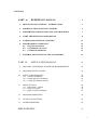
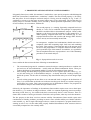
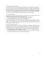
not be adapted in this manual either. Without entering into broad discussion on this matter, a strict distinction will be made between both terms. Let us consider a beam laid on some supports and loaded by
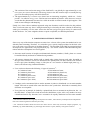
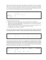
its own weight q, a variable force P and a constant axial force T, as shown in Fig. 1. The beam supports
are not fixed against vertical tension. This simple model can in principle be analyzed in 4 different ways
which are shown underneath in a matrix form, see Fig. 1.
Fig. 1. Convention of (non)linearity and (dis)continuity assumed in this manual
Observe that the division into continuous and discontinuous behavior runs across the one into linear and
non-linear one. The criterion is here a presence or an absence of slope discontinuities in the behavior
functions of the structure, not a linear or non-linear character of these functions. Strictly speaking, the
terms “continuous” and “discontinuous” are not quite correct here in the mathematical sense, as the
functions δ(P) remain continuous in all the four cases. They are only not smooth in the right half of the
matrix. These terms are, however, correct with respect to the first derivates (slopes) of these functions;
and – above all – correct in the physical sense. Loosing contact with beam supports introduces material
discontinuities in the system. In this – physical – sense we shall use these terms here.
3
In the considered example the continuous approach (both: linear and nonlinear) gives a tensile reaction
on the third support, which is obviously an error. Moreover, there is another, quite principal argument
in favor of discontinuous approach: Nature behaves in fact non-linear in a majority of problems. For no
other reason than our own convenience, we often approximate it by using linear or piecewise linear approach. The family of problems dealt with by DISCO represents a rather exceptional, opposite case:
Here the nature itself behaves piecewise linear (polygonal). There is no need to approximate it – it can
be modeled the way it behaves. In mathematical sense, polygon angles are slope discontinuities. Therefore, we will refer to them as “discontinuities”. In engineering, it is quite usual to refer in such a way to
sudden, sharp changes in structure properties, without explicit mentioning the word ‘slope’, see e.g. discussions on joints in shells of revolution by Roark [3] or by Bull [4]. In this sense one can distinguish
various types of discontinuities (or: discontinuous fixities):
•
•
•
•
•
external: e.g. discontinuous support conditions;
internal: e.g. ties or unfixed contacts between elements;
mechanical: caused by geometry or mechanical properties;
physical: caused by material properties, e.g. plastic hinges;
fractural: irreversible, caused by breakage, etc.
The DISCO algorithm presents a solution for structures with external discontinuities. An extension for
internal discontinuities and some other problems is possible and will briefly be discussed later on.
Engineering practice proves that a great majority of discontinuities occur at transition points between
negative and positive fixities of diverse degrees of freedom (DOF's). For clarity reasons this analysis is
limited to such cases. It is, however, a minor problem to program the levels of discontinuity as input
data, so that other than zero transition points can be defined. Such modification requires no further
changes to the presented algorithm.
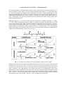
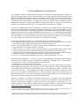
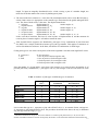
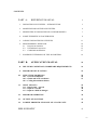
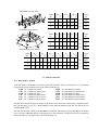
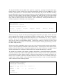
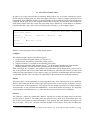
In Fig. 2 a number of polygonally linear problems have schematically been shown. Cases a until f represent discontinuous fixities of reaction forces in various directions; cases g and h are examples of discontinuous moment fixities. A short description follows below.
a.
b.
c.
d.
e.
f.
g.
h.
Suspensions of pipelines, tie-rod fixities of expansion joints;
Rails, crane driveways with limited tension fixities;
Cable stayed bridges, bustle pipes of steel works blast furnaces;
Cable stayed masts, towers, halls etc.;
Support rings e.g. of vertical pressure vessels, free laid foundation grids;
Concentrated loads on refractory lined oven shells, traffic tunnels etc.;
Single-sided moment fixities of columns and beams, torsion fixity of a blade;
Examples of discontinuous moment fixity in reinforced concrete.
4
Fig. 2. Examples of discontinuous fixity problems
5
2. MODELING DISCONTINUOS FIXITIES
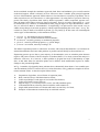
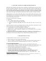
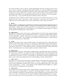
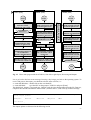
Note that all discontinuous fixities can be modeled by defining a "conditional" DOF, e.g.:
• force: tension fixed (#), compression free (0) – or reverse;
• moment: clockwise fixed (#), anti-clockwise free (0) – or reverse.
This also applies to DOF's that are not simply fixed or free, but that show different positive and negative fixity characteristics. The solution is then an additional, conditionally fixed element in the direction
of the considered DOF. This method can be illustrated by the three following examples (see Fig. 3).
Fig. 3. Modeling different fixity characteristics
In the first example a conditional spring has been used to model the elastic tension fixity of a beam support. In the second example two conditional springs represent different fixity characteristics of a column
base. (Note that the node coordinates of these springs can in fact be identical, as long as no connection
between them is defined.) The third example shows two ways of modeling discontinuous moment fixities. In that example, the two conditionally supported springs can optionally be fixed against displacement or against rotation.
This technique applies also to 3D-models where the number of conditional DOF's can be larger. The
limitation of the algorithm is, however, that only point-wise fixities can be defined in this way. A conditional line- (or surface-) support becomes released over a certain distance (or area) what makes the solution more complex. This can be solved by defining a number of conditional point-wise supports in a line
or over a surface. Such models are in fact powerful tools in solving numerous structural contact prob1)
lems (see e.g. Fig. 2 e and f), what has been illustrated in a practical case in section .
1)
Contact problems have been studied broadly in recent years. A linear incremental approach to such problems
has e.g. been presented by Simunovic and Saigal in [5]. Other approaches can e.g. be found in the works of Refaat and Meguid [6] or Wang and Nakamachi [7].
6
3. PROPERTIES OF DISCONTINUOUS LINEAR MODELS
Polygonally-linear (here called “discontinuous”) models have some special properties which distinguish
them from conventional, smooth-linear (“continuous”) models. The most favored property is, obviously,
that they allow for more adequate structural analyses. Having seen the examples in Fig. 2 and 3, it
would not be wrong to say that most structures behave more or less polygonally. The fact that they are
usually subject to ‘smooth’ modeling can be justified by limited precision requirements, narrow ranges
of load variation, our convenience, tradition etc.
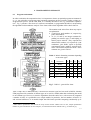
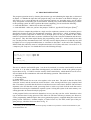
The second property is a warning: Separately computed load cases
should, as a rule, not be combined! The principle of superposition
should be considered false in discontinuous analyses. Observe what
happens to the beam from the beginning of this manual (Fig. 1)
when separately computed load cases are combined (Fig. 4). The
superposed deflected line and reactions (d) strongly differ from the
correct ones (a) and are mutually inconsistent.
In consequence, complete load combinations should each time be
computed, rather than computing single load cases and combining
the results. This property is important not only to the program users
but also to the programmers. A complete discussion on this subject
goes beyond the scope of this manual. Nevertheless, it’s significance
must de emphasized because superposition is one of the elementary
procedures in structural analyses.
Fig. 4. Superposition results in an error
Let us confine the discussion to the three following recommendations:
1.
2.
3.
The conventional programs for continuous structural analyses contain procedures to combine single load cases in load combinations – usually with user defined combination factors. These procedures should not be programmed (neither be used) for discontinuous linear analyses.
Most existing structural analysis programs make use of two separate input files called, e.g., system file and loading file. In discontinuous analyses - as already discussed - loadings actually codefine the systems. For the sake of consistency they should better make part of one integral input
file.
Several existing programs do not allow to set concentrated loads on supports in the directions of
fixity. It is assumed that such loads are irrelevant since they pass directly to reactions causing no
strain effect in a system. This is not necessarily true in discontinuous models. The programs for
discontinuous analyses must enable the input of those loads.
Obviously, the importance of loadings in discontinuous linear models requires more care to their input.
One should, e.g., be cautious in using load factors, which is a common engineering practice nowadays.
Increasing a load factor e.g. for variable loads does not necessarily lead to a safer structure. There is a
chance that a number of nodes get released or fixed after such operation, what may not be the intention.
The last property in this short overview concerns stability: Discontinuous linear models require more
consideration to stability problems, providing in return a more reliable stability test. Models which become unstable, e.g. due to single-sided support releases, cannot be computed. A program should issue a
warning in such a case. On the other hand, properly modeled discontinuous linear structures that are
successfully computed are also certainly stable.
7
4. SOME THEORETICAL BACKGROUND
Let’s consider a structure model meeting all Clapeyron’s conditions [8] and supported by a number of
point-wise external fixities (of forces and/or moments). Let’s assume that some of those fixities or all of
them are conditional (discontinuous) in the sense as discussed above. Since it is not known which singlesided fixities will be active and bear reactions, and which will be released - there is no way to solve this
discontinuous linear model directly. A solution must involve an iteration process eliminating released
fixities and converging in a model with a definite, ‘smooth’ fixity system. At each step of such iteration
an entire - let's call it after Ralston [9] - basic solution of the system must be computed.
A ‘classical’ nonlinear approach to such problems, as discussed e.g. by Bathe [1] (new supports arising
during structure deformation), considers the externally applied loads - thus also deformations, stresses
etc. - to be a function of time. The resulting approach is an incremental step-by-step procedure using the
solution for discrete time t to compute the solution for discrete time t + ∆t. Aside from the plea against
nonlinear approach as such (see Introduction), there are several practical reasons why this strategy has
been rejected here. For the space reasons, they are not discussed. Some of them (e.g. error accumulation, inconvenience of time functions) will become clear further in this manual.
The proposed algorithm of solution can, in the simplest terms, be described as follows:
1) Convert the structure model in such a way that all conditional (single-sided) fixities become unconditional (double-sided). Memorize conditional fixities in the original model.
2) Solve the converted model for the entire load combination, computing the vector of node displacements D and the vector of node external reactions R.
3) Check if every R ≠ 0 reaction occurs on the fixed side of a proper conditional DOF in the original
model. Each time it does not; modify the converted model by releasing the particular DOF.
4) Check if every D ≠ 0 displacement occurs on the free side of a proper conditional DOF in the original model. Each time it does not; modify the model by fixing the particular DOF.
5) If step 3 or 4 result in any modification, go to step 2. Otherwise the system is solved.
The question concerning step 1 is why to convert the single-sided DOF’s into double-sided. In general,
2)
two ways can be considered to convert a discontinuous model into a continuous one . Let us call them:
• Stiff approach: replace all single-sided fixities by double-sided;
• Slack approach: release all single-sided fixities.
A disadvantage of the slack approach is that it may produce an unstable model during the iteration.
This endangers the convergence. The stiff approach does not bear that risk. Another possible question is
why to bother checking the sides of displacements in step 4. One might suppose that – since the stiff approach has been used – it is the releasing of the DOF’s that leads to the solution, not the fixing. This
proves not to be sufficient. A DOF that has once been released may require to be fixed again in one of
the next iteration steps. As far as this approach has been researched, there exists no convergent iteration
that solves the problem using only irreversible DOF modifications.
Naturally, it should be proved that the procedure shown above is convergent. From the engineering
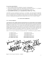
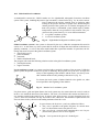
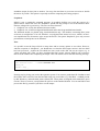
point of view, however, an instructive example is often more convincing than a strictly theoretical discussion. A simple model enabling to observe the features of the algorithm in a transparent way is a
weightless beam on a large number of rigid, tensionless supports, loaded by a single force in the middle
3)
of one span. In Fig. 5 a half of such a beam has been modeled due to the system symmetry .
2)
A third, "middle way" is also thinkable if additional precautions are taken to ensure the convergence. This
might lead to further perfectioning of the algorithm. It has not been investigated so far.
3)
This example requires an exceptionally large number of iterations. This and the problem triviality are chosen
deliberately to picture some features of the procedure. It must not be seen as a sign of its small efficiency.
8
Strain energy of
reactions [Nm]
Fig. 5. Iteration steps for a beam on tensionless supports – example
10
8
6
4
2
0
Step Step Step Step Step Step Step Step Step Step Step Step Step
0
1
2
3
4
5
6
7
8
9
10
11
12
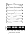
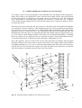
Fig. 6. Strain energy of reactions in the 12 iteration steps
(Energy level 0 equals here in fact 16.7 Nm, see calculations in the text)
9
As known, the solution of such a system is a free-supported one-span beam. The way, in which the algorithm described above comes to this solution, has been shown in steps 0 through 12. Note that each
step results in eliminating (sometimes also in adding) of a number of supports from which at least (here
always) one is eliminated definitely. That one support has each time been marked black in the drawing.
Note also that the supports guaranteeing the stability of the system (here just one) are not eliminated at
any step. These two features of the algorithm have been confirmed in a large number of tests on different systems. They are sufficient to make the procedure convergent.
We shall now follow the changes of strain energy “bound” by reactions in this iteration process. It is
convenient to do it in reverse order, in which we expect this energy to grow. Let‘s consider two
neighboring iteration steps i and i-1; and sign by j the joint (node) numbers of the beam. From the reciprocal theorem of Betti-Maxwell [8] we have:
∑ (P
n
j
j =1
+ Ri , j ) δ i −1, j = ∑ (Pj + Ri −1, j ) δ i , j .
n
j =1
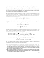
By proper modification of this equation we can obtain a double formula for work Li→ i-1 required to
bring the beam from the deformation state in step i back to the step i-1:
Li →i −1 =
1 n
∑ (Ri, jδ i−1, j − Ri −1, jδ i , j ) ,
2 j =1
Li →i −1 =
1 n
∑ Pj (δ i , j − δ i −1, j ) .
2 j =1
Since there are many reactions Rj and just one force Pj in our example, the easiest way to obtain strain
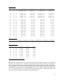
energy variation is through the second of these two equations. Starting from step 12, where the computed deflection under force P was δ = 3.33 mm, we obtain:
step 12, δ = 3.33 mm:
step 11, δ = 3.05 mm:
...
step 0, δ = 1.75 mm:
L12 = 12 × 10 × 3.33 × 10 −3 = 16.7 × 10 −3 kNm,
L12 →11 = 12 × 10 × (3,33 − 3,05) × 10 −3 = 1.4 × 10 −3 kNm,
L11 = (16.7 + 1.4 ) × 10 −3 = 18.1 × 10 −3 kNm,
...
L1→0 = 12 × 10 × (2.17 − 1.75) × 10 −3 = 2.1 × 10 −3 kNm,
L0 = (22.5 + 2.1) × 10 −3 = 24.6 × 10 −3 kNm.
The strain energy variation calculated in this way has been shown in a diagram in Fig. 6. There are
some interesting features to be observed in Fig. 5 and 6, namely:
• One can see that the elimination of the released DOF’s takes place in a quite regular, ‘frontal’ manner bearing, in this respect, some resemblances to other known elimination processes, e.g. to the
Gauss elimination.
• The DOF fixity, which becomes definitely eliminated, is here always the one, which “binds” the biggest strain energy. In more complex systems this will apply to certain groups of DOF’s rather than
the single DOF’s; which can make it less visible.
• We see that the total number of fixed DOF’s does not always become smaller at every step. Neither
the total strain energy of these DOF’s does always become smaller. See, e.g., the transition from step
7 to step 8. Yet, this does not endanger the convergence.
10
• The variation of the total strain energy of the fixed DOF’s can globally be approximated by a concave curve (arc convex downward). The energy losses in the first iteration steps are usually the biggest. This favorable property will still be discussed.
• The approximation by a concave curve shows here an interesting irregularity, which can – for the
present – be called an energy wave. This has not been studied any further. It has, however, been observed that this phenomenon becomes less visible in models on elastic instead of rigid supports. This
leads to some analogies with damping.
Finally, let’s observe that a nonlinear approach using time functions would be useless for this problem.
Time is irrelevant since any force P acting downwards gives basically the same solution (P directed upwards gives instability). For the same reason also the term polygonal approach may be controversial
for this load case. Yet, since weightless beams are quite exceptional, we shall drop that detail.
5. CODING DISCONTINOUS FIXITIES
Since every step of the iteration computes an entire basic solution of the system, the method can be considerably time-consuming. Therefore, it is advisable to use a quick, simple procedure for the basic solu4)
tion, even at the cost of diversity of modeling features . The algorithm of the DISCO program has been
developed for PC applications. The program itself [10] - uses a basic solution where the following limitations and other assumptions have been applied:
• Structure model consists of straight, one-dimensional elements (members). Shells, plates etc. can not
be modeled directly and must be simulated using members.
• All structure elements have default rigid or pinned nodes (joints) between each other, depended on
the type of the structure: Trusses are assumed to have pinned joints, all other structures are assumed
to have rigid joints. Modeling a hinge, a slide joint etc. in a structure of default rigid joints (e.g., a
frame) can be done using simulation members.
5)
• User can choose between the following 12 types of structures :
1 Continuous beam;
2 Discontinuous beam;
3 Continuous plane truss;
4 Discontinuous plane truss;
5 Continuous grid;
6 Discontinuous grid;
7 Continuous plane frame;
8 Discontinuous plane frame;
9 Continuous space truss;
10 Discontinuous space truss;
11 Continuous space frame;
12 Discontinuous space frame.
• Loadings can be concentrated (forces and/or moments in joints) or distributed over an entire member
length. All loads are stored in the same data files as the system data. Joint loads in externally fixed
directions are acceptable.
• Every joint can, in principle, be loaded by a pointed load (force or moment) in any direction, but – on
the other hand – to input such a load one must first define there a joint. Also every member can carry
a distributed load in any direction, but is assumed to be equally distributed over the entire member
4)
The discussed software was originally developed in the 1980’s, when memory consumption and computation
time were of more significance than they are today.
5)
For continuous models similar divisions have been used in some early structural analysis programs, e.g.
STRESS [11], ICES STRUNDL [12]. Such approach leads to a quick, memory saving basic solution.
11
length. To input an unequally distributed load or a load covering a part of a member length, one
must first divide the member into sectors by defining more joints.
• The result of the basic solution is a vector D of all joint displacements; and a vector R of all joint reactions. Both vectors are appropriate to the structure type and related to the global orthogonal XYZ
axes. The form of both vectors is the same. The displacements D are:
displacements DY,
rotation angles AZ;
• in beams:
displacements DX, DY;
• in plane trusses:
displacements DZ,
rotation angles AX, AY;
• in grids:
displacements DX, DY,
rotation angles AZ;
• in plane frames:
displacements DX, DY, DZ;
• in space trusses:
displacements DX, DY, DZ,
rotation angles AX, AY, AZ.
• in space frames:
In the vector R of reactions, the forces R come in place of displacements D, and the moments M
come in place of rotation angles A. All indices remain the same.
• Joint external fixities (supports) are identified by joint types. Every combination of joint fixed and
free DOF's has a unique (within the structure type) joint type number. This applies to continuous as
well as discontinuous structures. In the latter, the number of combinations is much larger.
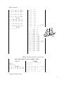
Coding joint types is one of the crucial points of the entire algorithm. Note that each single DOF can be:
If continuous:
1. free;
2. fixed.
If discontinuous:
1. free on positive and on negative side;
2. free on positive, fixed on negative side;
3. fixed on positive, free on negative side;
4. fixed on positive and on negative side.
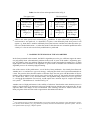
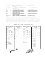
Since the number ND of joint DOF's varies from 2 for beams to 6 for space frames, the number NT of
possible joint fixity combinations (= joint types) will vary still stronger. This has been shown in Table
1:
Table 1. Numbers of joint types in different types of structures
No. (ND) of
DOF's
No. (NT) of joint types
Continuous
Discontinuous
2
4 = 16
2
4 = 16
3
4 = 64
3
4 = 64
3
4 = 64
6
4 = 4096
Beam
2
2 = 4
Plane truss
2
2 = 4
Grid
3
2 = 8
Plane frame
3
2 = 8
Space truss
3
2 = 8
Space frame
6
2 = 64
2
2
3
3
3
6
Let's assume that type no. 1 represents a joint with all DOF's free, i.e. no external fixities; and type no.
NT represents a joint with all DOF's fixed. The procedure described below shows the way to determine
6)
any joint type from the range [1..NT] :
6)
The Pascal notation for ranges is used in this manual. A notation [a..b] means here (a ÷ b) or a till b, included. The DISCO software has been developed by the author in Turbo Pascal® of Borland International Inc.
12
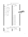
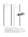
1. Make a table for the type of structure under consideration, with in the headline all DOF's as listed
earlier in this section. The tables for discontinuous structures should have double ("positive" and
"negative") columns under each DOF. In the most complex case of a space frame, the headlines of
such tables should be similar to the ones shown in Table 2.
Table 2. Examples of joint type determination in 3D-frames
- Continuous space frame:
Z
Joint
no.
Y
DX
5
2
26
X
DY DZ AX AY AZ
4
3
2
1
0
2 2 2 2 2
#
#
58
#
#
#
134
#
#
#
#
#
#
#
Type
no.
+1=
22
+1=
57
+1=
64
- Discontinuous space frame:
Joint
no.
25
- DX +
11
10
2 2
- DY +
9
8
2
2
- DZ +
7
6
2
2
#
#
#
129
138
#
#
#
#
#
#
#
#
- AX +
5
4
2
2
#
- AY +
3
2
2
2
- AZ +
1
0
2
2
#
#
#
#
#
#
#
#
#
#
Type
no.
+1=
4041
+1=
1345
+1=
4096
2. Assign to each column an integer value varying...
• for continuous models:
• for discontinuous models:
N D −1
0
2 N −1
0
from 2
down to 2 ,
from 2 D down to 2 ,
as shown for space frames (ND = 6) in the table headlines above (Table 2).
3. List all the fixed joints (supports) of the considered model in the left column; and check the cells
representing joint fixities e.g. by #. The sums of values assigned to the checked cells, increased by
7)
1, represent the joint types .
It is not difficult to see resemblances to the binary system in this coding. An advantage of such coding in
computer programming is that it enables the use of very quick, bit-level operations for all the transitions
from discontinuous to continuous fixities (joint types), and for all the modifications of joint types in the
8)
iteration process . The details of this will be discussed in the next section.
7)
In a computer program this procedure can e.g. be realized by using overlay windows. Checking ‘fixed’ cells can
then take place by a mouse click.
8)
In the past the binary code was used much wider to program the analyses of complex structural problems. An
impressing example of such notation can e.g. be found in [13]. This is, obviously, not the case here any more.
13
6. PROGRAMMING APPROACH
6.1
Program environment
In order to minimize the computation time, it is important to choose an optimal program environment. It
is, e.g., not advisable to incorporate time consuming operations on files (opening, reading, writing etc.)
in the iteration process. On the other hand, it is certainly advisable to use, e.g., band matrix optimiza9)
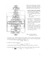
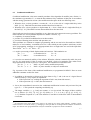
tion . Fig. 7 presents a flow chart of a software environment, as programmed in DISCO, incorporating
the algorithm for discontinuous analysis. Flow charts of the actual algorithm will be shown later on.
The notation used in this flow chart may require
an explanation:
• N and M are total numbers of, respectively,
joints and members.
• NC, ND, NS and NQ are integer constants depending on structure type TS and helping to
format proper matrices. They represent the
characteristic numbers of, respectively: joint
coordinates, joint DOF's (equal to possible
concentrated loads), member sectional stiffnesses and member distributed loads. These
constants are given in Table 3.
Table 3. Matrix formatting constants depending
on structure types
TS
Structures
NC
ND
NS
NQ
1, 7
Beams
1
2
1
1
2, 8
Plane trusses
2
2
1
0
3, 9
Grids
2
3
2
1
4, 10
Plane frames
2
3
2
2
5, 11
Space trusses
3
3
1
0
6, 12
Space frames
3
6
4
3
Fig. 7. DISCO – general flow chart
Table 3 helps also to understand why a division into structure types has been used in DISCO. Modern
FEM programs offer a number of element types to be used in a model rather than conforming the model
to one element type. However, in iterative algorithms where the entire basic solution must be computed
a number of times, it is preferable to use simple models. In particular, the low numbers of DOF's ND
and sectional stiffnesses NS in models simpler that 3D-frames speed the computing considerably up. It
9)
Band matrix optimization falls beside the scope of this manual. DISCO uses an own, simple optimization
method. A good introduction to more complex, so-called fractorization methods can e.g. be found in [9].
14
also keeps the band matrix [14], [15] narrow, limitting the memory consumption. Further, the following
features should be observed in the flow chart in Fig. 6:
• The entire input data for each run (loading case) is contained in one input file. No division into, e.g.,
system and loading files has been made. According to the discussion in section 3, no procedures
combining single loading cases into complex, superposed cases have been programmed.
• In the input data, the loadings have the same status as the so-called system data. Vector Fi[ND] of
joint i concentrated loads comes in fact right behind the vector of joint coordinates Ci[NC]. Vector
Qj[NQ] of member j distributed loads follows the vector of member stiffnesses Sj[NS].
• In case of odd type number TS (see structure types earlier in this manual), the structure is continuous
and there is no need for iteration. The first approach leads directly to the solution. In case of even TS
, the structure is discontinuous. It is first converted into a continuous structure. After the band matrix optimization, it undergoes an iteration process with joint type modifications at every step, converging in a solution that meets all discontinuous fixity conditions.
• The iteration process is memory- and time-saving. Note that no operations on files are involved. The
vector of joint reactions Ri[ND], which rules the process along with joint displacements Di[ND], becomes only computed for the joints of types TC,i > 1; and always to the same memory space.
• Compared to “continuous programs”, the flow chart in Fig. 7 contains only two really new blocks,
marked unconditional conversion and conditional modification. These blocks represent the essence
of the algorithm and will be discussed further in this section.
• With the exception of discontinuous analysis, this approach does not differ much from some early
programs for skeletal structures, e.g. STRESS [11]. However, it is a minor problem to adapt it to a
more complex FEM environment.
The block unconditional conversion converts all discontinuous joint types TD[N] into continuous ones
10)
TC[N] . As result the structure model becomes in fact Continuous. The vector of discontinuous joint
types TD[N] remains in memory for the boundary tests at each step of the iteration.
These tests are performed in the block conditional modification. The tested objects are vectors of joint
reactions Ri[ND] and displacements Di[ND]. In general, the procedure investigates whether reactions
have only been computed on the fixed sides, and displacements on the free sides of single-sided supports. Each time the answer is "no" a proper DOF gets released, respectively fixed for the next iteration
step.
6.2
Unconditional conversion
Unconditional conversion defines the initial model for the iteration. All discontinuous joint types TD,i are
replaced by continuous types TC,i in such a way that fixity on any side (+ or -) of a considered DOF
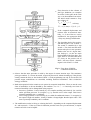
qualifies this DOF as fixed. This procedure is shown in a flow chart in Fig. 8. It does not make part of
the iteration process and is only executed once at the beginning of the program. Nevertheless an effort
has been done to minimize the computation. One of the measures applied is the introduction of a logical
variable Fix which provides exits from different loops as soon as their tasks are completed.
10)
Converting into continuous types means here converting into type coding of a continuous model, using the
stiff approach. E.g., the type number of an entirely fixed (i.e. in fact continuous) joint of a discontinuous space
frame changes from TD,i = 4096 into TC,i = 64, see examples in section 5.
15
Below are some other features of the flow
chart in Fig. 8. The comments concerning
programming approach apply largely to
the next flow chart in this manual as well:
• In order to speed up the computing,
binary operations are used, given here
in the Turbo Pascal® notation. Two
of them may require an explanation:
• i shl j shifts the value of i by j bits
to the left;
• i shr j shifts the value of i by j
bits to the right.
• The conversion is only activated for
joint types TD,i > 1. Logical, because if
TD,i = 1 then TC,i = 1. All entirely free
joints (usually a majority in structure
models) are in this way skipped, what
fastens the procedure.
• The integer variables i, u, v, g, h and j
are counters. Here are their ranges, in
case the bit-level code presents some
survey problems: i[1..N], u[1..2ND],
v[1..ND], g[1..NT] (binary i.e. 1, 2, 4,
8, etc.), h[1..g], j[1..NT/2u].
Fig. 8. Flow chart of DISCO
unconditional conversion
• The counters u and v match discontinuous fixities (negative, positive or both) of joint DOF's with
appropriate continuous ones. In simple terms: Each time u “spots” a fixity in a joint type number
TD,i, v increases the appropriate continuous type number TC,i by:
2 N D −v or binary: 1 shl ( N D − v) .
• The counter g is actually a function of u:
g = 2 u −1 or binary: g = 1 shl (u − 1),
and represents the column values in tables of discontinuous joint type numbers (see section 4).
• The counters h and j help u to find whether there is a fixity in these columns. This is the case when:
TD ,i =
NT h
− j + 1 or binary: TD ,i = ( N T shr (u − 1)) * h− j + 1 .
2 u −1
16
6.3
Conditional modification
Conditional modification is the most essential procedure of the algorithm. It modifies joint i fixities, i.e.
the continuous type numbers TC,i, to meet the discontinuous fixity conditions of that joint. In accordance
with the strategy presented in section 4, the modification takes place in the two following cases:
1. When the basic solution produces a reaction Ri,v ≠ 0 on a free side of a single-sided fixity in the
DOF v[1..ND]. That DOF becomes then modified from fixed in into free.
2. When the basic solution produces a displacement Di,v ≠ 0 on a fixed side of a single-sided fixity in
the DOF v[1..ND]. That DOF becomes then modified from free into fixed.
Since both cases involve testing of equalities to zero, there may arise numerical accuracy problems. The
nature and the size of such problems depend on a number of factors, e.g.:
• complexity of structure models;
• presence of so-called ill-conditioned areas in these models;
• precision of floating point variables and operations, etc.
These problems are common in computer programming and do not need to be discussed here. DISCO
makes use of two boundary ‘considered-to-be-zero’ values which proved to produce satisfactory results
in PC-programming, assuming no very disproportional force or length units are used in the input data.
-8
-6
11)
These values are: ε1 = 10 and ε2 = 10 .
ε1 is used in zero-testing of both: displacements and reactions. The boundaries are:
is considered to be:
Di,v = 0;
Di,v < ε1
is considered to be:
Ri,v = 0.
Ri,v < 1000 ε1
ε2 is used to test numerical stability of the solution. When the solution is numerically stable, the products Di,v* Ri,v must equal 0. If this is not the case, the DOF v fixity of a particular joint i must not undergo modification in order to preserve convergence. The boundaries used in DISCO are:
DOF v of joint i stable, modification possible;
Di,v* Ri,v  < ε2 →
DOF v of joint i instable, no subject to modification.
Di,v* Ri,v  ≥ ε2 →
Fig. 9 presents a flow chart of the conditional modification, as programmed in DISCO. Here are some
additional comments on this flow chart:
• In addition to the notation as discussed by flow charts in Fig. 7 and 8, the use of a logical Pascal
function Ord(expr.) may require an explanation:
• If the expression expr. making the argument of Ord is true, then Ord returns 1;
• If the expression expr. is false, then Ord returns 0.
• Just as the unconditional conversion, the conditional modification becomes only activated for joint
types TC,i > 1. This speeds the computing considerably up.
• The integer variables u, v, g, h and j are counters; w is a sign switch. The ranges of these variables
are as follows: u[1..2ND], v[1..ND], g[1..NT] (binary i.e. 1, 2, 4, 8, etc.), h[1..g], j[1..NT/2u], w[1,+1]. With the exception of w, the same notation is used here as in the flow chart of unconditional
conversion.
11)
In exceptional cases, these values may require to be tuned up. For more output stability, variable ‘considered-to-be-zeros’ can also be used, e.g. belonging to the input data or resulting from the analysis of numerical
input. This has not been programmed but it may be considered in prosperous versions of DISCO.
17
• Fixity detection in the columns of
joint type definition (see examples
in section 5) takes place in the same
way as in unconditional conversion.
The initial model contains a fixity
in a column u if:
NT h
− j + 1 , or binary:
2 u −1
= ( N T shr (u − 1)) * h− j + 1 .
TD ,i =
TD ,i
• If the computed displacement and
reaction show no numerical instability, i.e. if one of the two can be
considered 0, the appropriate DOF
v fixity may undergo modification.
• The algorithm checks first positive,
and then negative side of DOF v.
The switch is controlled by a sign
switch w. The check and the modification take place in one operation,
thanks to the use of a logical function Ord(expr.), see the two main
blocks middle in the flow chart. The
upper block is activated when there
is a fixity on the positive side of
DOF v; the lower block - when the
negative side of DOF v is fixed.
Fig. 9. Flow chart of DISCO
conditional modification
• Observe that the entire procedure is ruled by the output of current iteration steps. The continuous
joint type numbers TC,i become increased, respectively decreased, without checking up if they do not
already contain the fixity or the freedom of DOF v. Such programming can only be successful if all
possible output combinations are controlled, including numerical instabilities. This is indeed the
strategy in DISCO.
• Both main operation blocks contain an exit option for numerical instabilities. These are not the same
form of instabilities as the one handled by the condition Di,v* Ri,v  < ε2. Basically, two forms of
numerical instability can be distinguished in the program:
• Inaccuracy problems: Caused usually by too complex modeling and relatively low variable
and/or operation precision. To recognize, e.g., by unstable zero’s in the output. This form is
primarily handled by the ε1-conditions.
• Out of range problems: Caused usually by so-called ill-conditioned features. To recognize by
the output of high real numbers, usually a number of ranges higher than the input values. This
form is primarily handled by the ε2-condition.
• The modification results in fixing or releasing the DOF v, depending on the computed displacement
Di,v and reaction Ri,v. If the use of the Ord-function presents some survey inconveniences, a simpler
notation in Table 4 can be helpful:
18
Table 4. Action of two main operation blocks in Fig. 8
Ri,v ≤ 1000 ε1
Ri,v > 1000 ε1
Di,v ≤ ε1
Positive side
loaded, correct.
No change.
Releasing v.
TC,i decreases
N −v
by 2 D
Di,v ≥ -ε1
Fixing v. TC,i increases by
2 N D −v
Numerical instability, exit.
No change.
Di,v < -ε1
The lower block:
Di,v > ε1
The upper block:
Ri,v ≥ -1000 ε1
Ri,v < -1000 ε1
Releasing v.
Negative side
loaded, correct. TC,i decreases
N −v
No change.
by 2 D
Fixing v. TC,i
increases by
2 N D −v
Numerical instability, exit.
No change.
• There is one more special case covered by the ε-conditions. It arises when both: displacement Di,v
and reaction Ri,v are equal to 0, i.e. when DOF v of joint i is not effected by load in any sense. It can
appear e.g. when there is another sufficiently fixed joint between i and the load, when the entire system is not loaded in direction v, or when the strains in this direction are in internal equilibrium in the
vicinity of i. Also in such case no fixity modification is performed.
7. POSSIBLE EXTENSIONS OF THE ALGORITHM
In the form presented in this manual, the DISCO algorithm proved to give sufficient support in numerous polygonally linear (discontinuous) problems in the recent 16 years of the author’s engineering practice. Nevertheless, there are problems which can possibly be better approached in another way, or which
might require some extensions to the algorithm. A good reason to consider such extensions is that the
algorithm proves to be relatively high performing.
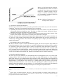
One of the sources of this performance - use of the fast, binary arithmetic - has already been discussed.
Another one is a simultaneous approach strategy - analyzing the whole set of system discontinuities at
a time. The practice shows that the number of iteration steps does not grow with the number of discontinuities (with exception of some trivial cases as the beam in section 4), but usually becomes stabilized
at a certain level. This is a very favorable feature. An algorithm using a kind of successive approach,
i.e. solving the discontinuities successively, would require more iteration steps for complex discontinu12)
ous systems . This difference is visualized in Fig. 10.
Another source of high performance is the stability of solutions. Note that the entire iteration process is
ruled by logical algebra; no numerical values are passed from one iteration step to the next one. In consequence, there is no danger of error accumulation. This advantage will not be found in diverse nonlinear programs which are often used to approximate discontinuous behavior.
12)
This comparison has not been studied further but a certain analogy can be drawn to the performance of iterative (Jacobi, Gauss-Seidler [14], [15]) and direct (Gauss) solutions of simultaneous equation systems. The first
ones perform better by large, complex systems.
19
Below is a brief discussion on extensionand modification ideas which can still be
considered. These ideas have not yet been
tested in a computer program. The discussion is therefore somewhat speculative. Nevertheless, it might be helpful to
prospective programmers:
Fig. 10. Number of iterations in two
strategies of the analysis
• Extension for internal discontinuities:
Member begin- and end joints can be given joint type numbers in the similar way as for the external discontinuities. Then the two programming strategies can be considered:
1. Expanding unconditional conversion and conditional modification in such a way that all (internal
and external) fixities are handled at a time. This leads to a single level iteration, probably the fastest.
Additional convergence precautions may then be needed.
2. Dividing the procedure: Each step of ‘external’ fixity iteration contains then an entire ‘internal’ fixity
iteration. Such a double level iteration is probably slower but better convergent.
Naturally, in internal fixity modifications the global joint displacements should be used as boundary values, not zeros. This presents some problems since these displacements may as well be effected by discontinuously connected members. The iteration will probably require a deeper joint analysis then pre13)
sented in this manual .
• Discontinuous edge- or surface supports:
In order to simulate a linear or surface discontinuous support, the user has to input a large number of
pointed discontinuities. This can, obviously, be avoided by defining special contact interfaces, modules
etc., allowing to input entire contact edges or surfaces as single items. Such procedures are known e.g.
14)
to generate complex finite element types , and do not need to be discussed here. This extension seems
to be convenient for large FEM programs, running on networks with powerful central units. DISCO has
been programmed for a small stand alone PC with a limited operation memory (the used Turbo Pascal
version can not address more than 64 kB), therefore it made little sense to extend it in that way.
• Mutually related discontinuities:
In section 4, four fixity conditions of a discontinuous DOF are distinguished. This covers most forthcoming problems. There are cases, however, where fixity of a single DOF depends on a fixity of another
DOF rather than on a sign of displacement in the same DOF. In the sample problem presented further in
this manual, it would probably be more convenient to relate the fixity of rotation angle AZ to the fixity of
displacement DX. Such relations can be realized e.g. by adding another joint type number - this time for
mutually related discontinuities - to the current one; and expanding the conditional modification. For
mutually related discontinuities the type numbers > TD can possibly be used. Since such discontinuities
are seldom, a proper detection could be performed prior to entering the expanded routines.
13)
A quite deep analysis, based however on a different, incremental search algorithm, has been presented in
[22].
14)
Special types of complex elements, which are in fact used nowadays to simulate contact problems, are
boundary elements [23]. In particular the hybrid methods combining finite- and boundary element approach
[24], [25] have been successful in this field.
20
• Other than zero discontinuity levels:
As already mentioned, it is a minor problem to install other than zero discontinuity levels. Instead of (or
next to) detecting positive and negative displacements and reactions, the algorithm would distinguish between the values below and above certain levels, which should then be specified in the input data. Also
this possibility will not be used often in structural engineering, but it can be helpful e.g. in simulations
of plastic hinges, supports on buoyancy tanks etc. It can not be used for modeling fracture problems
(e.g. cracks), as the algorithm handles only polygonal behavior, where there is just one function value
for each argument. In fracture problems more values are possible for a single argument.
• Fracture discontinuities:
The above does not necessarily mean that no routines of the algorithm can be adapted in fractural discontinuity analyses. Especially interesting for this purpose can be:
1. The binary technique of coding joint types (the number of types might be larger);
2. The so-called stiff approach (see section 4) and the unconditional conversion;
3. Conditional modification in an internal iteration within a load step.
In general, it looks promising to use the discussed routines within the user defined load steps in fracture
analyses. As the algorithm does not contribute to error accumulation, this will probably lead to ‘fine
tuning’ of load step results. The error accumulation effect can in this way be limited to inaccuracies at
transition points between the load steps.
• Non-linear polygonal problems:
In non-linear polygonal analyses (see discussion on terminology at the beginning of this paper) a strategy opposite to the one mentioned above seems more promising: Use the non-linear routines within the
algorithm iteration steps. Such approach would possibly lead to a very accurate, multi-purpose structural analysis programming. However, the following two problems should be taken into consideration:
1. The non-linear procedures must then be highly accurate as well. Their error should in principle not
exceed the boundaries set by the ε-conditions, see section 6.3.
2. In case of large displacements, some extra precautions may be necessary to ensure convergence.
Convergence problems are, however, not new in non-linear analysis.
21
CONTENTS
PART A:
REFERENCE MANUAL
2
1.
DISCONTINUOUS FIXITIES – INTRODUCTION
3
2.
MODELING DISCONTINUOUS FIXITIES
6
3.
PROPERTIES OF DISCONTINUOUS LINEAR MODELS
7
4.
SOME THEORETICAL BACKGROUND
8
5.
CODING DISCONTINUOUS FIXITIES
11
6.
PROGRAMMING APPROACH
6.1. Program environment
6.2. Unconditional conversion
6.3. Conditional modification
14
14
15
17
7.
POSSIBLE EXTENSIONS OF THE ALGORITHM
19
PART B:
APPLICATION MANUAL
22
8.
DELIVERY CONDITIONS, HARDWARE REQUIREMENTS
23
9.
PROGRAM INSTALLATION
23
10.
STRUCTURE MODELING
10.1 General assumptions
10.2 Global and local coordinates
10.3 Coding discontinuous fixities
24
26
27
11.
INPUT OF DATA
11.1 Data format – general
11.2 Input in a text file
11.3 Input in a DISCO dialogue
29
29
30
36
12.
PROGRAM OPERATION
39
13.
OUTPUT OF SOLUTION
41
14.
SAMPLE PROBLEM: LEAKAGE OF A LOCK GATE
43
BIBLIOGHAPHY
47
22
8. DELIVERY CONDITIONS, HARDWARE REQUIREMENTS
DISCO has been developed by the author with no contribution of any third parties of persons. The author does not intend to register this software or to take any other steps to protect his rights and/or distribute his product commercially. As this software has been enclosed to the doctor’s thesis submitted at
the Civil and Environmental Engineering Department of the Gdansk University of Technology (further
called ”the University”), the University owns now its copy rights. As such, the University may take
steps to protect these right, and/or impose any distribution or other restrictions according to its policy.
Although utmost care was taken to debug this software, nor the author neither the University can be
held responsible for any consequences of its applications. In particular, users are warned that unprofessional modifications of the included Pascal and text files (e.g. intended to adapt third party lay-outs)
may cause the damage of the software.
The software is delivered in a set containing:
• this manual;
• one 3½” diskette named ‘DISCO’ and containing:
• system files in directories DISCO and DANCE;
• data files in directories CBE, DBE, CPT, DPT, CGR, DGR, CPF, DPF, CST, DST, CSF,
DSF.
As the first software versions were developed in the late 1980’s, the hardware requirements are quite
mild in relation to the current standards. What the user needs, is only:
• PC running under any version of MS Windows or MS DOS;
• hard disk in drive C:\ with about 1 MB memory space for the DISCO system files;
• graphical card “on board” enabling the emulation of one of the following cards: CGA, MCGA,
EGA,VGA or Hercules;
• diskette drive, USB port or any other data storage device – as long as it is configured to be A:\.
The delivered software version can not address a data storage port other than A:\. It is also not tailored
for running in a network system, although it can be adapted to that by a skilled professional.
9. PROGRAM INSTALLATION
To install the DISCO software on your PC, please do the following:
1. Make a back-up copy of your original DISCO diskette.
2. Take a new diskette, a USB memory key or any other data storage medium assigned to drive A:\,
15)
and copy all data file directories (CBE through DSF) into it. Label it, e.g., “DISCO data” .
For operation under MS Windows:
3. Insert your DISCO diskette into a disk drive of your PC. Get its directory on the screen.
4. Use MS Windows Explorer to copy the entire directories (names and contents) DISCO and
DANCE into drive C:\ (Attention: Not into C:\Programs or any other directory on drive C:\).
5. Click on C:\DISCO and get its directory on the screen.
6. Link (shortcut) the DISCO.EXE file to your MS Windows desktop
(Attention: Not the DISCO files with other extensions, e.g. PAS, BAK).
7. Link (shortcut) the DANCE.BAT file (MS DOS batch file) to your MS Windows desktop
(Attention: Not the DANCE files with other extensions, e.g. EXE, PAS, BAK, TXT).
8. Get your desktop screen, insert the DISCO data disk in drive A:\, click on DISCO and … Voila!
15)
Further in this manual, we shall talk about “data disk” and “drive A:\” only. However, it refers also to, e.g.,
“USB data key ” and “port A:\” if this is the configuration of your computer.
23
For operation under MS DOS:
3. Insert your DISCO diskette into a disk drive of your PC. Get the prompt C:\.
4. Copy the entire directories (names and contents) DISCO and DANCE into drive C:\, e.g. using the
DOS Xcopy /s command (Attention: Not into any other directory on drive C:\).
5. Log into the DISCO directory , e.g. by typing CD \DISCO and pressing <Enter>.
6. Insert the DISCO data disk in drive A:\, type DISCO, press <Enter> and … Voila!
Your DISCO system is operational now and you can – in principle – start processing the example data
files on your data disk and computing their solutions You can also input and compute your own data
files. It is advisable, however, to read the rest of this manual first. In particular, deleting the supplied
data files or modifying them through the DISCO dialogue may result in a loss of valuable examples.
10. STRUCTURE MODELING
10.1. General assumptions
As discussed in section 5, DISCO performs structural analyses for structure models of twelve different
types. Therefore, you should first choose the type which suits your problem the best. Keep in mind that
the higher your structure type number will be, the more complex and memory consuming computation it
will require. In extreme cases, i.e. by very large space frame models, the program may even run out of
memory. Special program architecture and the use of a band matrix optimization take care that this does
not happen soon. Exact limits can not be given, but space frames up to about 150 nodes (joints) and 200
members should, in general, successfully be computed. For other types of structures, these limits usually exceed 800. The only programmed limitation is no more than 999 joints and 999 members.
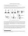
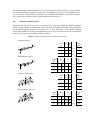
There are six basic types of structures to be chosen from (Fig. 11), divided into two groups as follows:
1
3
5
7
9
11
Continuous beam;
Continuous plane truss;
Continuous grid;
Continuous plane frame;
Continuous space truss;
Continuous space frame;
a)
Z
1
4
3
2
5
6
Y
b)
X
3
1
e)
12
9
Y
11
8
10
4
7
6
3
4
10
7
Z
f)
X
17
14
15
12
d)
11
2
12
17
16
14
13
Z
7
16
9
8
3
2
1
10
4
11
5
12
X
6
Z
X
14
13
18
15
16
6
7
8
1
11
Y
X
15
10
1
8
Y
18
Y
13
5
2
2
13
9
5
1
15
14
6
3
X
Z
Y
Z
9
7
5
Discontinuous beam;
Discontinuous plane truss;
Discontinuous grid;
Discontinuous plane frame;
Discontinuous space truss;
Discontinuous space frame.
c)
8
6
4
2
2
4
6
8
10
12
5
9
3
4
Fig. 11. Six basic types of structures – examples
24
The structure geometry must be input in a global right-handed (Cartesian) coordinate system. For the
types 1 ÷ 8 (a ÷ d in Fig 11), the position of the global coordinate axes is partly predefined by assuming
that the structure must lie in the global XY plane. For beams, types 1 and 2 (a in Fig. 11), the additional
assumptions are that the global X axis coincides with the beam, the loads act in the global XY plane,
and the joints and members are sequentially numbered in the positive direction of X. For the types 9 ÷
12 (e and f in Fig. 11), any position of the global coordinate system can be chosen.
The difference between continuous and discontinuous structures has been discussed in section 1 of this
manual. The terms “beam”, “plane truss”, “grid”, “plane frame”, “space truss” and “space frame” are
widely known. To avoid confusion, however, here is how DISCO sees these types of structures:
a) Beams
Beams are linear, straight structures, supported by any number of pointed supports fixing any degree of
freedom (DOF) or a combination of DOF’s. The DOF’s of a beam node (joint) are deflection Dy and rotation angle Az . Beams can be loaded by pointed forces Fy and moments Mz , as well as by member (in
DISCO equally) distributed loads qy . Beam members can have different sectional rigidity EIz , which is
the only parameter determining their flexural behavior.
b) Plane trusses
Plane trusses are 2D structures built of linear, straight members with all joints (also supports) hinged.
The DOF’s of a plane truss joint are displacements Dx and Dy . Any number of DOF fixities (supports)
or their combinations is possible. Plane trusses can only bear pointed loads in joints. These loads are
force components Fx and Fy . Truss members can have different sectional rigidity EAx , which is the only
parameter determining the truss deformation.
c) Grids
Grids are 2D structures built of linear, straight members with rigid internal joints; and loaded perpendicularly to the structure plane. The DOF’s of a grid joint are displacement Dz and rotation angles Ax
and Ay . Grids can be supported by any number of joint DOF fixities or their combinations. The possible
grid loads are joint force Fz , joint moments Mx and My , and member (in DISCO equally) distributed
load qz . Grid members have two sectional rigidities: torsional GIx and flexural EIy .
d) Plane frames
Plane frames are 2D structures built of linear, straight members with rigid internal joints; and loaded in
the structure plane. The DOF’s of a plane frame joint are displacements Dx and Dy and a rotation angle
Az . Also plane frames can be supported by any number of joint DOF fixities or their combinations. The
possible loads are joint forces Fx and Fy , joint moment Mz , and member (in DISCO equally) distributed
loads qx and qy . Plane frame members have two sectional rigidities: axial EAx and flexural EIz .
e) Space trusses
Space trusses are 3D structures built of linear, straight members with all joints (also supports) hinged.
The DOF’s of a space truss joint are displacements Dx , Dy and Dz . Any number of DOF fixities (supports) or their combinations is possible. Space trusses can only bear pointed loads in joints. These loads
are force components Fx , Fy and Fz . Truss members can have different sectional rigidity EAx , which is
the only parameter determining the truss deformation.
f) Plane frames
Space frames are 3D structures built of linear straight members with rigid internal joints. The DOF’s of
a space frame joint are displacements Dx , Dy and Dz , and rotation angles Ax , Ay and Az . Space frames
can be supported in any number of joint DOF fixities or their combinations. The possible loads are joint
forces Fx , Fy and Fz , joint moments Mx , My and Mz, and member equally distributed loads qx , qy and qy .
Space frame members have four sectional rigidities: axial EAx, torsional GIx and two flexural EIy and EIz.
25
10.2. Global and local coordinates
As mentioned in section 10.1, DISCO makes use of a right-handed, orthogonal (Cartesian) coordinate
system. This system, including the positive sign convention, is shown below (Fig. 12). In can be convenient to memorize the positive rotation signs as clockwise when
Z
looking in the positive direction of proper axes. Memorizing the
mutual position of the system axes is essential. Swapping two of
them will produce a left-handed system which requires another
ΦZ
interpretation than the one presented in this manual. The program uses the system from Fig. 12 in two different manners:
• as a global coordinate system;
O
ΦX
ΦY
• as a local coordinate system.
X
Y
Fig. 12. Right-handed orthogonal coordinate system
Global coordinate system is the system as allocated by the user, within the assumptions discussed in
section 10.1. As the name says, that system shall be used for all input data and solution results that are
globally orientated, i.e. refer to the entire model rather than a particular member. In particular, the following data must be input in the global coordinate system:
• joint fixities (types);
• joint coordinates;
• joint loads;
• member distributed loads.
The program will return the following solution results in the global coordinate system:
• joint displacements;
• support reactions.
Local coordinate system is a system associated with a particular member of the structure. Unlike the
global system, the position of the local system is defined by the program, nor by the user. Its origin lies
always in the beginning of the member; and the local x axis always coinz
cides with the member itself, pointing at the end of it (Fig. 13).
y
o
For beams, the local system is further identical to the global one, when
moved parallel to the beginning of the member.
end
beginning
x
Fig. 13. Member local coordinate system
For plane trusses, grids and plane frames, the local system may also rotate about the z-axis in order to
let the x-axis match the direction of the member. The local y-axis follows this rotation and the local zaxis remains parallel to the global Z-axis. In trusses (also space trusses), you may forget the local axes
y and z, since truss members can only bear loads in the x-direction. The members of plane frames can
also bear shear in the y-direction and bending moments about the z-axis.
z
y
Z
B
y
Y
X
z
B
x
x
E
E
x
E
E
x
z
B
y
B
z
y
In space frames, the local axes y and z are defined as follows:
• The y-axis is parallel to the global XY-plane. In vertical members it is directed the same as the global Y-axis.
• The z-axis lies in a vertical plane containing the x-axis. Its projection on the global Z-axis is never negative.
Fig. 14. Local system in the posts of a football goal
26
This definition applies when the global Z-axis is vertical, which is an advised choice. A good example
of it is the determination of local axes in the posts of a football goal, see Fig. 14. If the global Z-axis is
not vertical, than “vertical members” should be read as members perpendicular to the global XY-plane;
and “vertical plane” should be read as plane parallel to the global Z-axis.
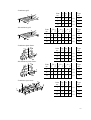
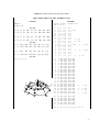
10.3.
Coding discontinuous fixities
As discussed in section 5, each joint of your structure has a joint type number that defines its external
fixities. It must explicitly be included into your input data. The method to determine joint type numbers
has globally been shown, using the most complex case – a space frame joint – as an example. Following
are the table headlines for joint type determination in all 12 types of structures that can be computed by
DISCO, along with some calculation examples (Tables 5):
Table 5. Joint type determination in 12 types of structures
- Continuous beam:
Joint
no.
X
Z
1
3
2
5
4
6
Type
no.
DY AZ
1
0
2
2
1
/
#
+1=
2
2
#
/
+1=
3
6
/
/
+1=
1
Y
- Discontinuous beam:
X
Z
5
1
4
3
2
6
Y
Joint
no.
- DY +
3
2
2
2
- AZ +
1
0
2
2
Type
no.
1
#
#
#
/
+1=
15
3
#
/
/
/
+1=
9
4
/
#
/
/
+1=
5
- Continuous plane truss:
Joint
no.
Y
9
7
5
3
1
6
4
2
8
X
Z
DX DY
1
0
2
2
Type
no.
1
/
#
+1=
2
5
/
/
+1=
1
9
#
#
+1=
4
- Discontinuous plane truss:
Joint
no.
Y
1
6
4
2
3
8
5
9
7
Z
- DX +
3
2
2
2
- DY +
1
0
2
2
Type
no.
1
/
/
#
/
+1=
3
5
#
/
#
#
+1=
12
9
#
#
#
#
+1=
16
X
27
- Continuous grid:
9
5
1
2
10
6
4
3
7
Z
14
15
16
12
11
8
Joint
no.
X
13
Y
DZ AX AY
2
1
0
2 2 2
Type
no.
1
#
#
#
+1=
8
7
/
/
/
+1=
1
13
#
/
/
+1=
5
- Discontinuous grid:
5
1
2
6
4
3
7
Z
14
12
11
8
- DZ +
5
4
2
2
- AX +
3
2
2
2
- AY +
1
0
2
2
1
#
#
#
#
#
#
+1=
64
4
/
#
/
/
#
/
+1=
19
16
/
#
#
/
/
/
+1=
25
Joint
no.
X
13
9
15
16
Y
Type
no.
- Continuous plane frame:
Y 18
17
15
14
13
8
7
1
2
Joint
no.
16
9
11
10
3
6
5
4
X
12
Z
DX DY AZ
1
0
2
2 2
2
Type
no.
1
/
#
#
+1=
4
9
/
/
/
+1=
1
12
#
/
/
+1=
5
- Discontinuous plane frame:
Y 18
17
16
15
14
13
8
7
1
2
Joint
no.
9
10
5
4
3
X
11
12
6
Z
- DX + - DY +
3
2
5
4
2
2
2 2
- AZ +
1
0
2
2
Type
no.
1
/
/
#
/
#
#
+1=
12
9
/
/
/
/
/
/
+1=
1
12
/
#
/
/
#
/
+1=
19
- Continuous space truss:
12
Z
6
3
Y
2
9
13
10
4
1
X
14
11
8
5
15
7
Joint
no.
DX DY DZ
2
1
0
2
2 2
Type
no.
1
#
#
#
+1=
8
2
#
/
#
+1=
6
13
/
#
#
+1=
4
28
- Discontinuous space truss:
15
12
Z
9
14
6
3
Y
11
8
13
5
10
2
7
4
1
- DX + - DY +
3
2
5
4
2
2
2 2
- DZ +
1
0
2
2
1
#
/
/
/
#
/
+1=
35
2
/
/
#
/
#
/
+1=
11
13
/
#
#
#
#
/
+1=
31
Joint
no.
X
Type
no.
- Continuous space frame:
18
17
Y
15
10
11
2
Joint
no.
X
14
6
7
8
1
Z
16
13
12
5
9
4
3
DX DY DZ AX AY AZ
5
4
3
2
1
0
2
2 2 2 2 2
Type
no.
3
#
#
#
/
/
/
+1=
57
4
/
#
#
/
/
/
+1=
25
5
#
/
#
/
/
/
+1=
41
- Discontinuous space frame:
- DX + - DY +
9
8
11
10
2
2
2 2
- DZ +
7
6
2
2
3
#
#
#
#
#
#
/
/
/
/
/
/
+1=
4033
4
/
/
#
/
#
/
/
/
/
/
/
/
+1=
641
5
/
#
/
/
#
/
/
/
/
/
/
/
+1=
1153
Joint
no.
- AX +
5
4
2
2
- AY +
3
2
2
2
- AZ +
1
0
2
2
Type
no.
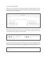
11. INPUT OF DATA
11.1. Data format - general
Your data must be submitted in a text file (a file with extension .TXT), stored in drive A:\ on a diskette
or other data storage medium in one of the following directories:
\CBE for Continuous beams;
\DBE for Discontinuous beams;
\CPT for Continuous plane trusses;
\DPT for Discontinuous plane trusses;
\CGR for Continuous grids;
\DGR for Discontinuous grids;
\CPF for Continuous plane frames;
\DPF for Discontinuous plane frames;
\CST for Continuous space trusses;
\DST for Discontinuous space trusses;
\CSF for Continuous space frames;
\DSF for Discontinuous space frames.
The data file names have the same names as the names of the directories, followed by a sequential number from the range [1..99]. E.g., the full address of the first discontinuous grid data file will always be:
A:\DGR\DGR1.TXT
The data file consists of three parts that must be submitted, followed by one part that may be submitted
in case you like additional details on the behavior of some members. All these parts must be separated
from each other by a single free line. The data file parts are:
29
•
•
•
•
General data:
16)
project and/or structure name, force and length units, total numbers of joints and members .
Joint data:
per input line: joint type, joint global coordinates, joint concentrated loads.
Member data:
16)
per input line: beginning and end joint , sectional rigidities, member distributed loads.
Members for extended output:
member numbers of for detailed output of extreme deflections and bending moments.
Observe that this data combines the data about structure geometry and stiffness with the data about
structure loads. The latter not only do not make a separate ‘loading file’, but they are even given in the
same input lines as the first. This would be surprising in computer programs performing a conventional,
“continuous” analysis, but is a logical and deliberate step in DISCO. In discontinuous analyses, superposition of different loading cases is – by definition – an error, because loadings co-define the systems,
see discussion in section 3. Therefore, no provisions should be made to encourage such a superposition.
11.2. Input in a text file
The data file can be prepared in two different manners:
• Using a text editor which can process the *.TXT files;
• Using the DISCO own interactive input dialogue.
The first way is faster and offers better review possibilities for a skilled program user. It may, however
be less convenient for a beginner. As the only test of the data is then the program run itself, it may cost
a number of runs before the data file is debugged. The second way is slower and offers less review possibilities, but it makes it almost impossible to produce a file resulting in a runtime error. That way will
be discussed in the following section.
There are a number of text editors which can process *.TXT files. All computers working under the MS
Windows operating system are, e.g., standard supplied with a WordPad editor. This editor produces and
processes the *.TXT files. Such files are also produced by a range of old text editors running under the
MS DOS operating system. Also the compilers of popular high-level computer languages contain editors of such files. The author, e.g., wrote his first data files in the editor of Borland’s Turbo Pascal®,
the same compiler that was used to develop and test the actual program.
Let us assign:
Project
Fu
Lu
n
m
i
j
Ti
X, Y, Z
x, y, z
lj
16)
=
=
=
=
=
=
=
=
=
=
=
name of the project, loading case etc.
force units, e.g.: kN, N, T, kG, Lb
length units, e.g.: m, cm, mm, ft, in
number of joints
number of members
sequential joint number
sequential member number
type number of joint I
global coordinates X, Y and Z
local coordinates x, y and z
length of member j
– string up to 56 characters;
– string up to 2 characters;
– string up to 2 characters;
– positive integer < 999;
– positive integer < 999;
– positive integer < n;
– positive integer < m;
– positive integer, see section 10.3;
– real values in Lu;
– real values in Lu;
– positive real value in Lu;
The number of members is superfluous for beams. In beams, this number equals the number of joints, minus
one. The member beginning and end joints are also superfluous there, as the joints are numbered sequentially.
30
FXi, FYi, FZi =
joint i concentrated force loads
in global axes
= joint i concentrated moment loads
about global axes
beginning and end joint of member j
section axial rigidity of member j
section torsion rigidity of member j
section bending rigidity of member j
about the local y-axis
section bending rigidity of member j
about the local z-axis
member j distributed loads in global axes
MXi, MYi, MZi
bj , ej
EAx,j
GIx,j
EIy,j
=
=
=
=
EIz,j
=
qXj, qYj, qZj =
– real values in Fu;
– real values in Fu·Lu;
– positive integer < n;
– positive real value in Fu;
– positive real value in Fu·Lu2;
– positive real value in Fu·Lu2;
– positive real value in Fu·Lu2;
– real values in Fu/Lu;
With the exception of the data Project that occupies a whole input, all other data have to be sorted out
in lines and separated from each other by one or more blanks (no commas!). Below (Tables 6 ÷ 10) are
the data formats for the six types of structures from section 10.1. The only difference between continuous and discontinuous data files (not mentioning their names) is that the continuous joint types TCi
change into the discontinuous ones TDi , as shown in section 10.3. The data in brackets […] are optional.
If you, e.g., only want to enter the second of them, you must – obviously – enter a zero for the first.
Table 6. Format of data files for beams and plane trusses
Beams (files CBE*.TXT and DBE*.TXT):
General
Example
Project
Fu Lu n
free line
T1 X1 [FY1 MZ1]
T2 X2 [FY2 MZ2]
……
Ti Xi [FYi MZi ]
……
Tn Xn [FYn MZn]
free line
EIz1 [qy1]
EIz2 [qy2]
……
EIzj [qyj ]
……
EIzm [qym]
free line
[j1 j2 j3 j4 …]
Beam - Figure 11a
kN m 6
2 0
3 2
3 6
3 10
0
3 14
1 16 -10
2E4
2E4 -4
2E4
2E4
2E4
2 3 4
15
Plane trusses (files CBE*.TXT and DBE*.TXT):
General
Example
Project
Fu Lu n m
free line
T1 X1 Y1 [FX1
T2 X2 Y2 [FX2
……
Ti Xi Yi [FXi
……
Tn Xn Yn [FXn
free line
b1 e1 EAx1
b2 e2 EAx2
……
bj ej EAxj
……
bm em EAxm
X
Z
1
2
Y
3
4
5
Truss - Figure 11b
kN m 9 15
FYi ]
FYn]
4
2
1
3
0.0
3.0
6.0
9.0
12.0
15.0
18.0
21.0
24.0
1
3
5
7
2
4
6
1
2
3
4
5
6
7
8
Y
6
2
1
1
1
1
1
1
1
4
FY1]
FY2]
5
3
5
7
9
4
6
8
2
3
4
5
6
7
8
9
0.0
5.0
0.0
5.0
0.0
5.0
0.0
5.0
0.0
0 -100
0 -100
50
-50
1E6
1E6
1E6
1E6
1E6
1E6
1E6
5E5
2E5
2E5
2E5
2E5
2E5
2E5
5E5
8
6
9
7
X
Z
31
Table 7. Format of data files for grids
Grids (files CGR*.TXT and DGR*.TXT):
General
Example
Grid - Figure 11c
kN m 16 24
Project
Fu Lu n m
T1 X1
T2 X2
……
Ti Xi
……
Tn Xn
free line
Y1 [FZ1 MX1 MY1]
Y2 [FZ2 MX2 MY2]
Yi [FZi MXi MYi ]
Yn [FZn MXn MYn]
free line
GIx1 EIy1 [qz1]
GIx2 EIy2 [qz2]
b1 e1
b2 e2
……
bj ej GIxj EIyj [qzj ]
……
bm em GIxm EIym [qzj ]
free line
[j1 j2 j3 j4 …]
8
1
1
8
1
1
1
1
1
1
1
1
5
1
1
5
0
0
0
0
5
5
5
5
10
10
10
10
15
15
15
15
1
2
3
5
6
7
9
10
11
13
14
15
1
2
3
4
5
6
7
8
9
10
11
12
2
3
4
6
7
8
10
11
12
14
15
16
5
6
7
8
9
10
11
12
13
14
15
16
0
3
6
9
0
3
6
9
0
3
6
9
0
3
6
9
0 -50
2E4
2E4
2E4
2E4
2E4
2E4
2E4
2E4
2E4
2E4
2E4
2E4
5E4
5E4
5E4
5E4
5E4
5E4
5E4
5E4
5E4
5E4
5E4
5E4
5
1
75
2
Z
4E5
4E5
4E5
4E5
4E5
4E5
4E5
4E5
4E5
4E5
4E5
4E5
1E6
1E6
1E6
1E6
1E6
1E6
1E6
1E6
1E6
1E6
1E6
1E6
3
13
9
6
4
10
7
8
11
X
14
12
15
16
Y
20
Table 8. Format of data files for plane frames
Plane frames (files CPF*.TXT and DPF*.TXT):
General
Example
Plane frame - Figure 11d
kN m 18 22
Project
Fu Lu n m
free line
Continued on the next page…
32
Table 8 continued:
T1 X1
T2 X2
……
Ti Xi
……
Tn Xn
4
4
4
4
4
4
1
1
1
1
1
5
1
1
1
1
1
1
Y1 [FX1 FY1 MZ1]
Y2 [FX2 FY2 MZ2]
Yi [FXi FYi MZi ]
Yn [FXn FXn MZn]
free line
EAx1 EIz1 [qX1 qY1]
EAx2 EIz2 [qX2 qY2]
b1 e1
b2 e2
……
bj ej EAxj EIzj [qXj qYj ]
……
bm em EAxm EIzm [qXm qZm]
free line
[j1 j2 j3 j4 …]
1
2
3
4
5
6
7
8
9
10
11
7
13
15
12
14
16
9
10
13
15
17
12
-6.0
-4.0
-2.0
2.0
4.0
6.0
-6.0
-4.0
-2.0
2.0
4.0
6.0
-4.0
4.0
-3.0
3.0
-3.0
3.0
7
8
9
10
11
12
8
9
10
11
12
13
15
17
14
16
18
13
14
14
16
18
13
-0.2
-0.2
-0.2
-0.2
-0.2
-0.2
0.0
0.0
0.0
0.0
0.0
0.0
3.0
3.0
6.0
6.0
9.0
9.0
2.0E3
2.0E3
2.0E3
2.0E3
2.0E3
2.0E3
8.0E5
8.0E5
8.0E5
8.0E5
8.0E5
2.0E5
2.0E5
2.0E5
2.0E5
2.0E5
2.0E5
1.2E5
1.2E5
2.0E6
2.0E6
2.0E6
0
0 -50
0
0 -50
0 -75
20
1.0
1.0
1.0
1.0
1.0
1.0
6.0E4
6.0E4
6.0E4
6.0E4
6.0E4
5.0E3
5.0E3
5.0E3
5.0E3
5.0E3
5.0E3
1.0E4
1.0E4
1.8E5
1.8E5
1.8E5
Y 18
17
16
15
14
13
7
1
8
2
9
3
10
4
11
5
12
X
6
Z
16.0
18.0
20.0
14
Table 9. Format of data files for space trusses
Space trusses (files CST*.TXT and DST*.TXT):
General
Space truss – Figure 11e
kN m 15 39
Project
Fu Lu n m
T1 X1 Y1
T2 X2 Y2
……
Example
free line
Z1 [FX1 FY1 FZ1]
Z2 [FX2 FY2 FZ2]
8
8
1
1
1
1
0.0 -2.0
0.0 2.0
0.0 0.0
4.0 -2.0
4.0 2.0
4.0 0.0
0.0 0
0 -40
0.0 0
0 -120
5.0 50
0.0 0
0 -80
0.0
5.0 0 -30
Continued on the next page…
33
Table 9 continued:
Ti Xi Yi Zi [FXi FYi FZi ]
……
Tn Xn Yn Zn [FXn FXn FZn]
free line
b1 e1 EAx1
b2 e2 EAx2
……
bj ej EAxj
……
bm em EAxm
1
1
1
1
1
1
8
8
1
8.0 -2.0
8.0 2.0
8.0 0.0
12.0 -2.0
12.0 2.0
12.0 0.0
16.0 -2.0
16.0 2.0
16.0 0.0
1
4
7
10
2
5
8
11
3
6
9
12
1
4
7
10
13
1
2
4
5
7
8
10
11
13
14
3
2
6
5
7
9
10
12
1
4
8
11
4
7
10
13
5
8
11
14
6
9
12
15
2
5
8
11
14
3
3
6
6
9
9
12
12
15
15
4
6
7
9
12
11
15
14
5
8
10
13
2.0E5
2.0E5
2.0E5
2.0E5
2.0E5
2.0E5
2.0E5
2.0E5
4.0E5
4.0E5
4.0E5
4.0E5
1.0E6
1.0E6
1.0E6
1.0E6
1.0E6
5.0E4
5.0E4
5.0E4
5.0E4
5.0E4
5.0E4
5.0E4
5.0E4
5.0E4
5.0E4
1.0E5
1.0E5
1.0E5
1.0E5
1.0E5
1.0E5
1.0E5
1.0E5
1.0E5
1.0E5
1.0E5
1.0E5
0.0 0
0 -80
0.0
5.0 0 -30
0.0 0
0 -80
0.0
5.0 0 -30
0.0 0
0 -40
0.0 0
0 -120
5.0 50
12
Z
9
3
2
11
8
5
X
14
6
Y
15
13
10
4
7
1
Regarding the input of real values, please observe the following:
•
•
•
•
The Anglo-Saxon notation should be used, i.e. with decimal points and not decimal commas.
If you use a decimal point, DISCO expects at least one digit behind it. For the notations like ‘10.’,
an error message will be returned.
You can choose between the decimal (e.g. 9.81) and exponential (e.g. 0.981E1) notation by each
individual data. Both positive and negative exponents are acceptable.
As the output will be returned in a decimal notation, it is advisable to choose such force and length
units that the results will form very long numbers. E.g. for a bridge, it is better to input in the data
kiloNewtons (kN) and meters (m) than in Newtons (N) and millimeters.
34
Table 10. Format of data files for space frames
Space frames (files CSF*.TXT and DSF*.TXT):
General
Example
Space frame - Figure 11f
kN m 18 29
Project
Fu Lu n m
T1 X1
T2 X2
……
Ti Xi
……
Tn Xn
b1 e1
b2 e2
……
bj ej
……
bm em
[j1 j2
free line
Y1 Z1 [FX1 FY1 FZ1 MX1 MY1 MZ1]
Y2 Z2 [FX2 FY2 FZ2 MX2 MY2 MZ2]
Yi
Zi [FXi FYi FZi MXi MYi MZi ]
Yn Zn [FXn
EAx1 GIx1
EAx2 GIx2
FXn FZn MXn MYn MZn]
free line
EIy1 EIz1 [qX1 qY1 qZ1]
EIy2 EIz2 [qX2 qY2 qZ2]
EAxj GIxj EIyj EIzj [qXj qYj qYj]
EAxm GIxm EIym EIzm [qXm qYm qZm]
free line
j3 j4 …]
18
17
Y
15
10
11
2
12
13
5
9
3
X
14
6
7
8
1
Z
16
57
1
57
25
41
41
57
1
1
1
1
1
1
1
1
1
1
1
-5.0
-5.0
-5.0
0.0
5.0
5.0
0.0
-4.5
-4.5
-4.0
-4.0
-4.0
0.0
4.0
4.0
4.0
0.0
0.0
2.9
0.0
-2.9
-5.8
-2.9
2.9
5.8
2.6
-2.6
2.3
0.0
-2.3
-4.6
-2.3
0.0
2.3
4.6
0.0
0.0
0.0
0.0
0.0
0.0
0.0
0.0
2.0
2.0
4.0
4.0
4.0
4.0
4.0
4.0
4.0
4.0
5.5
1
2
3
4
5
6
7
1
8
3
9
4
5
6
7
10
11
12
13
14
15
16
17
2
3
4
5
6
7
1
8
10
9
12
13
14
16
17
11
12
13
14
15
16
17
10
1E5
1E5
1E5
1E5
1E5
1E5
1E5
5E4
5E4
5E4
5E4
5E4
5E4
5E4
5E4
1E5
1E5
1E5
1E5
1E5
1E5
1E5
1E5
5E3
5E3
5E3
5E3
5E3
5E3
5E3
2E3
2E3
2E3
2E3
2E3
2E3
2E3
2E3
5E3
5E3
5E3
5E3
5E3
5E3
5E3
5E3
2E4
2E4
2E4
2E4
2E4
2E4
2E4
8E3
8E3
8E3
8E3
8E3
8E3
8E3
8E3
2E4
2E4
2E4
2E4
2E4
2E4
2E4
2E4
2E4
2E4
2E4
2E4
2E4
2E4
2E4
8E3
8E3
8E3
8E3
8E3
8E3
8E3
8E3
2E4
2E4
2E4
2E4
2E4
2E4
2E4
2E4
10
12
13
14
16
17
18
18
18
18
18
18
5E4
5E4
5E4
5E4
5E4
5E4
2E3
2E3
2E3
2E3
2E3
2E3
8E3
8E3
8E3
8E3
8E3
8E3
8E3
8E3
8E3
8E3
8E3
8E3
100
0 -50
0 80
150
0
0 120
0
0
0 120
0
0 -60
0
0 -20
0
0
0 -20
0 -20
0
0 -20
4
16 17 18 19 20 21 22 23 24 25
35
11.2. Input in a DISCO dialogue
DISCO offers also an opportunity to input the data interactively, in a dialogue with the user. This option requires some more key strokes, but it may still be convenient due to the built-in data control subroutines which will not let any incorrect value pass through. The dialogue begins already on the program opening screen, which looks like this:
Gdansk Institute of Technology - Faculty of Hydro & Environmental Engineering
------------------------------------------------------------------------------|
|
D I S C O
| ANALYSIS OF STRUCTURES WITH CONTINUOUS AND DISCONTINUOUS SUPPORT CONDITIONS |
------------------------------------------------------------------------------R.A. Daniel
Version 4/04
DISCO computes the following types of structures:
Continuously supported:
1
3
5
7
9
11
Continuous
Continuous
Continuous
Continuous
Continuous
Continuous
beam
plane
grid
plane
space
space
Discontinuously supported:
2
4
6
8
10
12
truss
frame
truss
frame
Discontinuous
Discontinuous
Discontinuous
Discontinuous
Discontinuous
Discontinuous
beam
plane
grid
plane
space
space
truss
frame
truss
frame
Your choice (0= Exit) : _
Make sure that the DISCO data diskette is in drive A:\ at this moment. You may now enter the type of
structure which you want to analyze. Let us assume that it is a continuous plane frame. Type 7 and
press [Enter]. The program response will be about as follows:
Available data files of this type:
1
3
5
Cpf1.txt: Cont. plane frame, EX1
Cpf3.txt: Small offshore rig
Cpf5.txt: Frame – Figure 11d
2
4
6
Cpf2.txt: Cont. plane frame, EX2
Cpf4.txt: Hartelkering, stijlen
Cpf6.txt: Free
Your choice (0= Exit) : _
If you want to process (Delete, Update, Append, Model, Output or Setup for computing) an existing
data file, you will enter its number (in this case 1..5). Take care not to do it when you intend to Input a
new file, as it will overwrite the existing one. We now discuss an entirely new input, therefore type 6
and press [Enter]. DISCO will then open a free file Cpf6.txt with only one processing option - Input:
Available processing options:
1
Input
Your choice (0= Exit) : _
36
Typing 1 and pressing [Enter] opens then the input dialogue, in which DISCO asks the succeeding data
about your structure; and you enter those data from the keyboard. If the entry is incorrect, the program
will not accept it, otherwise it will display it and ask you to confirm it by prompting ‘(Y/N)?’ behind.
You can change it then by pressing N or go to the next data by pressing Y. For the plane frame from
Fig. 11d, the screen will look as follows after the general data has been input:
Input
F1= Repeat
F2= Finish
Esc= Escape
Other= Go on
Cpf6.txt
-----------------------------------------------------------------------General data:
Project
Force units
Length units
No. of joints
No. of members
:
:
:
:
:
Plane frame – Figure 11d
kN
m
18
22_
Four options will appear in the top line:
• F1 makes the program go back to the entry ‘Project’ and repeat this part of the dialogue;
• F2 allows you to save the completed part of the input and go back to the previous screen, which
will now show 3 processing options: Delete, Update and Append. You can then press 0 to take a
break or use Append to resume your work,.
• Esc will erase all new input. If you are in the Input mode, it will erase the new opened file. If you
are in the Append or Update mode, it will only erase all additions or updates.
• Any other key will continue the Input dialogue.
Press, indeed, any other key which will bring you to the second part: the input of joint data. DISCO will
now ask the joint type, joint coordinates and joint concentrated loads for all succeeding joints, checking
every entry and asking you to confirm it. At the end of the first joint input, the screen will look like this:
Input
F1= Repeat
F2= Finish
Esc= Escape
Other= Go on
Cpf6.txt
-----------------------------------------------------------------------Joint data:
Joint
1 :
t =
FX=
4
0.000
X =
FY=
-6.000
0.000
Y =
MZ=
-0.200
0.000
The same four options appear now in the top line. Pressing F1 repeats the dialogue about this particular
joint; other options work as discussed above. Press any other key to go to joint 2, then joint 3 etc. When
all joint data has been input and you have not taken a break by pressing F2, DISCO will go to the third
part of the Input dialogue: the member data. You will now be asked to input in succession: the member
beginning and end joint, the axial rigidity EAx, the flexural rigidity EIz and the member distributed
loads. At the end of the first member input, the screen will look like this:
Input
F1= Repeat
F2= Finish
Esc= Escape
Other= Go on
Cpf6.txt
-----------------------------------------------------------------------Member data:
Member
1 :
from
7
EAx=
QX =
1
2000.000
0.000
to
EIz=
QY=
1.000
0.000
37
The keys F1, F2, Esc and any other allow again for, respectively, repeating the member data input,
breaking the job, erasing the entire new input and continuing the dialogue. Press any other key to go to
member 2, then member 3 etc. When all member data has been input and you have not taken a break by
pressing F2, DISCO will go to the fourth and last part of the Input dialogue: the members for extended
output. You will be asked to enter the numbers of members for which you like to receive the locations
and values of extreme deflections and/or bending moments. Entering those members proceeds in a dialogue similar to what has already been discussed – and is terminated by entering 0. When this is successfully completed, the following screen should appear:
Input complete
Cpf6.txt
-----------------------------------------------------------------------Your data file : Cpf6.txt
Available processing options:
1 Input
2 Delete
3 Update
4 Append
5 Model
6 Output
7 Setup
Your choice (0= Exit) : _
If there are less (e.g. only the first four) processing options at the end of your input, it means that some
incorrect data has been entered, not detected by the DISCO verifying routines. The program will usually
help you localize it, by issuing a message like “Bad joint 15” or “Bad member 20”. Use e.g. Update to
correct it. The use of a *.txt file editor – discussed in section 11.2 – is less convenient, because DISCO
stores all real values in an exponential notation, 11 digits long, which is as not easy to survey as the
decimal notation. For this reason, it is also better not to let it replace the data prepared using a text editor, unless really necessary.
Having successfully completed the input, you can now view the structure model using the option Model.
It gives a simple graphical presentation of the structure model – meant only for screen control, not for
printing. Using the option Output will produce another data file, called ‘LastDat.txt’, decently arranged
in tables and suitable for a hard print. This data file will be stored in the directory C:\DANCE.
The option Setup computes some memory constants and performs a simple band matrix optimization,
especially useful for large models which might otherwise cause a memory overflow. This optimization is
an original DISCO routine. Simply speaking, it divides the band matrix into a number of dynamic submatrices, most of which are narrower than the band matrix width. This saves the memory allowing to
compute more complex models. After performing Setup, the problem is ready for actual computation,
which is announced in the following manner:
- Computing memory constants
- Rock & Roll optimization
- Setting up for processing
DISCO set up for : Plane frame – Figure 11d
Joints
18
Members
22
- matrix 1 from
1 to 18,
band width
5
Run DANCE
Strike any key _
38
12. PROGRAM OPERATION
The program operation starts by choosing the structure type and submitting the input data, as discussed
in chapter 11. Whether the input has been prepared using a text file editor or the DISCO dialogue, you
still need to get a screen showing the seven processing options (see preceding page), run the option
Setup and get the screen telling you to run DANCE. Pressing a key closes DISCO and brings you back
to the operating system. In order to perform the actual computing, you can now do the following:
• under MS Windows: double-click on the icon DANCE;
17)
• under MS DOS: make sure you have the prompt C:\DISCO\, type DANCE and press [Enter] .
DISCO will now compute the problem in a single run (for continuous structures) or an iteration process
described in chapters 4 and 6 (for discontinuous structures). There will be a “cloud” of numbers flying”
through your screen, impossible to follow due to the high speed. Do not pay attention to that. These
numbers represent the band matrix structure at different steps of the Gaussian elimination and the iteration process. They had been helpful during the programming, when PC’s worked much slower than
now, but they became incommunicative later. The only reason to display them now is that they may still
be helpful in case of program modifications or extensions in the future. At the end of this computing,
DISCO finds the solution in terms of a displacement matrix of all joints; and stores it in on drive A:\ in
a temporary file Temp.txt. You should then receive the following message:
MODEL SOLVED
Setting up for output: Cpf6.txt
DISCO ready to output: Cpf6.txt
Run DANCE
Strike any key _
The user is asked to run DANCE again – but do not be confused, it is not the same DANCE as the one
in section 11.2. In order to understand what happened, you should take a look at the global program
layout shown in Fig. 15. DISCO consists actually of three main blocks, which should be run in succession and which do not communicate with each other during operation. These blocks are:
• Input block;
• Processing block;
• Output block.
Moreover, these blocks do not even exist together at the same time. The truth is that the first block
writes the second; and the second one writes the third – after erasing itself from your computer hard
disk. This makes it possible that the block two and three have the same names: DANCE. But still more
important is the fact that the second, processing block is in this way freed of all the tasks that can be
separated from solving the simultaneous equation system. Solving that system is the most memory consuming procedure in structural analysis programs.
As the program blocks erase and write themselves in every run, they can also “tailor” themselves to the
type of structure that is being processed. This allows for still more efficiency in memory use. However,
such a programming method requires that a new-generated program is compiled during the actual computing session. Therefore, a runtime compiler of Turbo Pascal 4.0, TPC.EXE, makes part of the program package, which has also been shown in Fig. 15.
17)
Obviously, you do not need to care about the prompt C:\DISCO if you add it to the PATH command in your
AUTOEXEC.BAT file.
39
DANCE [Enter]
DANCE [Enter]
START
START
INPUT OR REVIEW OF
DATA INCL. PRINT,
GRAPHICAL AND OTHER
COMPILING DANCE.PAS
FROM THE DESKTOP AND
STARTING EXECUTION
Y
DATA O.K.?
N
SAVING DATA FILE
SOLVING THE SYSTEM OF
EQUATIONS IN MATRICES
DEFINED BY DISCO.EXE
Y
COMPUTING MEMORY
ARRANGEMENTS, BAND
MATRIX OPTIMIZATION
START
BOUNDARIES O.K.?
SAVING DISPLACEMENTS
N
TPC.EXE OF TURBO PASCAL 4.0
BY BORLAND INTERNATIONAL
DISCO [Enter]
MODIFYIN
G FIXITIES
ERASING DANCE.PAS,
OPENING NEW DANCE.PAS
WITH COMPUTED
MEMORY ARRANGEMENTS
SELF-ERASING, OPENING
AND “TAILORING” A NEW
DANCE.PAS
ADDING FILE DANC1.TXT
TO COMPLETE DANCE.PAS
ADDING FILE DANC2.TXT
TO COMPLETE DANCE.PAS
END
END
COMPILING DANCE.PAS
FROM THE DESKTOP AND
STARTING EXECUTION
READING DISPLACEMENTS
SAVED BY OLD DANCE.PAS
COMPUTING REACTIONS
AND MEMBER FORCES
COMPILING DANCE.PAS
FROM THE DESKTOP AND
STARTING EXECUTION
COMPILING DANCE.PAS
FROM THE DESKTOP AND
STARTING EXECUTION
Y
OTHER OPTION ?
N
END
Fig. 15. Three main program blocks of DISCO, from left to right: Input, Processing and Output
Let us go back to the last screen message. Pressing a key brings you back to the operating system. To
receive and process the output, you should now do the same as before, i.e.:
• under MS Windows: double-click on the icon DANCE;
type DANCE on the prompt C:\DISCO\ and press [Enter].
• under MS DOS:
The third block, Output, is activated now. DISCO reads the joint displacements from the file Temp.txt,
computes the reactions and member internal loads (“member forces”) and comes up with the message:
Output for Plane frame – Figure 11d
Choose output option:
Complete
Partial
Selective
Graphical
Exit
Your choice: _
The output options are discussed in the following section.
40
13. OUTPUT OF SOLUTION
In order to save paper and spare the environment, DISCO allows you to view the solution first; and to
present only the essential parts of it in the final output. Therefore, a number of output options have been
programmed. Such additional facilities are possible thanks to the fact that the structure has already been
computed and the large part of the computer memory has been freed. The first three of the output four
main options shown in the last screen (one page back) can be delivered as screen output or as both the
screen and the disk output. Here is that screen again after choosing, e.g., the complete output:
Output for Plane frame – Figure 11d
Choose output option:
Complete
Partial
Selective
Graphical
Exit
Your choice: C
Screen
Hard disk + Screen
Your choice: _
Below is a short description of the available output options.
Complete:
The complete output consists of the following parts:
• Program headlines and general data (see section 11.1);
• Displacements and rotations of all nodes (called “joints”);
• Support reactions (i.e. reactions in all externally fixed joints);
18)
• Member internal loads (called “member forces” ) at the beginning and the end of each member;
• Bending extremes (extreme deflections and moments) in all earlier specified members.
After choosing C for “Complete”, the computer will output these data in decent tables, easy to survey.
Due to the problems with screen control under MS Windows by other than MS software, no data scroll
routine has been programmed. If your output is long, you can better use the H option first and examine
it in the hard disk file. There will still be an opportunity to shorten that file for the final presentation.
Partial:
This option gives you the opportunity to choose only those parts of the output that are of your particular
interest. The format and the size of the output parts are the same as in the option “Complete”, but you
can skip the parts of less significance. The program will ask whether a part has to be output (displayed
in Screen mode, or also put on the disk in Hard disk + Screen mode) before processing it. It is especially
useful for quick or limited analyses, e.g. when only the system reactions are to be considered.
Selective:
The “Selective” output goes further than “Partial”, allowing you to tailor the output exactly to the form
in which want to present it. The editing takes now place not only on the level of the output parts, but
also on the level of particular joints and members. After printing each table headline, the program will
ask you to enter – one by one – the joint or member numbers of your interest. Every entry is followed by
18)
This term, less common in Europe, is largely used in America, e.g. in the classical MIT programs [11], [12].
41
immediate output for that joint or member. You may also enter them in your own succession or double
the entries if you like. This option is especially useful for comparing and sorting purposes.
Graphical:
DISCO is not a graphically orientated program. Its graphical facilities serve only the purpose of a
global control. Also in this case, the “Graphical” option will only prompt a view of the structure deformations, enlarged for a good survey. The user can chose between:
• Graphical view of only the deformed structure model;
• Graphical view of in the background undeformed, and in the foreground deformed model;
The deformed models are plotted using joint deformations only. The members connecting those joints
are drawn as straight lines. You will, therefore, see polygonal lines instead of curves, which is an obvious simplification for all structure types except the trusses. The option “Graphical” gives only a screen
presentation; no hard prints can be obtained.
Exit:
It is possible to run the Output block as many times and in as many options as one wishes. However,
with the exception of “Graphical”, you should take care that the final output version is the last which
has been processed – anyhow the last which has been saved on the disk. Do not run Output (e.g. to
“check one thing still”) after you have completed the final version, because DISCO will overwrite it
then. Press E for Exit after completing the output. This will end the session with the following message:
Your data output file: C:\DANCE\LastDat.txt
Your solution file:
C:\DANCE\LastSol.txt
Thank you.
Strike a key: _
Pressing any key brings you back to the operation system. You can now get the data file LastDat.txt and
the solution file LastSol.txt from the hard disk using any word editor (e.g. WordPad – standard present
by MS Windows); and make hard prints of those files. These prints are skipped in this manual for space
reasons. There is, however, an input data file cpf5.txt on the attached diskette. You can run DISCO and
process this file by yourself if you like to see the output.
42
14. SAMPLE PROBLEM: LEAKAGE OF A LOCK GATE
The complex system of water management in the Netherlands faces the designers with still higher demands. One of them is the construction of locks with mitre gates which can bear water pressure from
both sides: the pointed, so-called positive side and the concave, so-called negative side. The second load
case is unfavorable, as water tends then to open the gate instead of - as in the first case - keeping it
closed. Despite leakage problems the idea wins still more support since it reduces the number of necessary mitre gate leaves.
The most recent project where this idea has been used, is the check gates of the double lock-aqueduct
over a motorway, Naviduct Enkhuizen. This remarkable project gives a free navigation passage between
two large lakes, IJsselmeer and Markermeer, which originate from the damming of the ancient Dutch
internal see, Zuiderzee, in the early 1930’s. The construction of this project was completed in 2003. The
detailed design of the mitre gates was performed using the finite element analysis program DIANA [16],
[17]. The contact- and the leakage problems of the gates were investigated using DISCO. Combining
these two programs in one design proved to be successful in author’s earlier hydrotechnical projects,
e.g. the storm surge barrier on the Hartel Canal in the harbor of Rotterdam [18], [19].
Due to the symmetry, only one of leaf of the Naviduct mitre gate had to be modeled. Since the global
geometrical behavior was of prior interest, not the local stresses, the computer model used by DISCO
was highly simplified (Fig. 16). It was a 3D-frame model with the main body of the leaf in one plane.
Only the drive arm lever and the line support to the other leaf did not lay in that plane. All elements
were linear members; all internal joints were rigid, each with 6 DOF’s.
Fig. 16. Structural analysis model for one of the two gate leaves
43
When closed, the gate drive cylinders prestress the gate with a force Fy,1 ≤ 1000 kN in order to limit the
opening which appears along the contact line under negative hydraulic load. This prestression results in
19)
a compression of the UHMPE edge lining. The resultant of the hydraulic load acts some meters lower,
20)
tending to open the gate. Due to the complex torsional rigidity of the gate , it is impossible to determine the effective contact length directly as an input data. This problem has been solved using a row of
conditional elastic supports which can only bear compression, see joints no. 41 through 60. When tension is computed, these joints become released to show the widths of a leakage gap between the two
leaves. The gap between the bottom members and the threshold is computed simultaneously.
Table 11 presents some input excerpts for a negative water head (fall) of 1.0 m, which is a maximum
for this lock operation. By larger falls (1.0 to 3.0 m) the navigation holds up, the negatively faced gate
goes open and the opposite, positively faced gate bears the entire load. Yet, the negative fall of 1.0 m
presents a more severe problem due to the leakage.
For demonstration reasons, some more types of discontinuous fixities have been modeled. The second
one concerns the fixity of a rotation angle AZ along the contact line. In the upper part, above water, the
buffer is in fact twice as wide as underneath in order to sustain frequent prestression. When the whole
gate deflects, the compressed contact line will have a fixed rotation about the Z-axis. Since the E2
modulus of UHMPE is low (~300÷500 N/mm ), this effect can practically be ignored, but let’s assume
that we like to see it in the stiffer upper part only. It can be done by fixing both sides of the rotation angle AZ in that part. However, just for demonstration, single-sided rotation fixities have been used: The
upper part (first 4 supports) is fixed against the positive AZ rotation, which is expected to occur. The
lower part (remaining 16 supports) is fixed against the negative AZ rotation, which is not expected in
this case. Finally, there is a single-sided fixity of a vertical displacement in a pivot bearing under the rotation axis (joint no. 8): downwards fixed, upwards free. A double-sided pinned support would be correct here as well since there is no doubt about the sign of the vertical support reaction. However, this is
not always clear in more complex structures and/or load cases.
Table 11. Sample problem - input excerpts
Joint data:
Joint Type
1
2
3
1
3841
1
. . . . . . .
7
1
8 3969
9
1
. . . . . . .
41 1026
42 1026
43 1026
44 1026
45 1027
46 1027
. . . . . . .
58 1027
59 1027
60 1027
19)
20)
X(m)
Y(m)
Z(m)
-DX+
-DY+
-DZ+
-AX+
-AY+
-AZ+
-2.033
0.000
0.000
1.455
0.000
0.000
6.550
7.100
6.550
/
#
/
/
#
/
/
#
/
/
#
/
/
/
/
/
/
/
/
/
/
/
/
/
/
/
/
/
/
/
/
/
/
/
/
/
0.000
0.000
1.101
0.000
0.000
0.366
0.530
0.000
6.550
/
#
/
/
#
/
/
#
/
/
#
/
/
#
/
/
/
/
/
/
/
/
/
/
/
/
/
/
/
/
/
/
/
/
/
/
6.657
6.657
6.657
6.657
6.657
6.657
2.181
2.181
2.181
2.181
2.181
2.181
6.850
6.550
6.170
5.790
5.410
5.030
/
/
/
/
/
/
#
#
#
#
#
#
/
/
/
/
/
/
/
/
/
/
/
/
/
/
/
/
/
/
/
/
/
/
/
/
/
/
/
/
/
/
/
/
/
/
/
/
/
/
/
/
/
/
/
/
/
/
/
/
#
#
#
#
/
/
#
#
#
#
/
/
6.657
6.657
6.657
2.181
2.181
2.181
0.530
0.265
0.000
/
/
/
#
#
#
/
/
/
/
/
/
/
/
/
/
/
/
/
/
/
/
/
/
/
/
/
/
/
/
/
/
/
/
/
/
Ultra High Molecular Polyethylene.
The torsional rigidity is built up by diagonals between beam rear flanges. In a plane model this can be simulated e.g. using the approach presented by Kollbrunner [20] or Dąbrowski [21].
44
Member data:
Member From To
1
2
1
2
3
3
. . . . . . .
29
9 13
30
10 14
31
13 19
32
19 22
33
5 15
34
15 20
. . . . . . .
58
21 41
59
22 42
60
23 43
61
24 44
62
25 45
63
26 46
64
27 47
65
28 48
66
29 49
67
30 50
68
31 51
69
32 52
70
33 53
71
34 54
72
35 55
73
36 56
74
37 57
75
38 58
76
39 59
77
40 60
EAx(kN)
GIx(kNm²)
EIy(kNm²)
EIz(kNm²)
10710000.000
10550000.000
2536.000
158000.000
43200.000
21000000.000
738600.000
222200.000
7346000.000
7346000.000
7346000.000
7346000.000
7480000.000
7480000.000
564.800
56070.000
564.800
564.800
157700.000
111100.000
21000000.000
21000000.000
21000000.000
21000000.000
21000000.000
21000000.000
417900.000
417900.000
417900.000
417900.000
249100.000
249100.000
25100.000
25100.000
25100.000
25100.000
13700.000
13700.000
13700.000
13700.000
13700.000
13700.000
13700.000
13700.000
13300.000
13300.000
13300.000
13300.000
13300.000
11500.000
9500.000
18000.000
100.000
100.000
100.000
100.000
100.000
100.000
100.000
100.000
100.000
100.000
100.000
100.000
100.000
100.000
100.000
100.000
100.000
100.000
100.000
100.000
1000.000
1000.000
1000.000
1000.000
1000.000
1000.000
1000.000
1000.000
1000.000
1000.000
1000.000
1000.000
1000.000
1000.000
1000.000
1000.000
1000.000
1000.000
1000.000
1000.000
101.100
101.100
101.100
101.100
16.400
16.400
16.400
16.400
16.400
16.400
16.400
16.400
15.900
15.900
15.900
15.900
15.900
13.700
11.500
21.600
Joint loadings:
Joint
Type
FX(kN)
FY(kN)
FZ(kN)
MX(kNm)
MY(kNm)
MZ(kNm)
1
1
0.000
0.000
1000.000
0.000
0.000
-220.000
0.000
0.000
0.000
0.000
0.000
0.000
1
15
Member loadings:
Member From To
33
34
35
36
37
38
39
40
41
42
43
5
15
20
6
16
7
8
11
12
17
18
15
20
27
16
32
11
12
17
18
38
40
QX(kN)
QY(kN)
QZ(kN)
-10.590
-5.280
-5.280
-22.950
-22.950
-4.180
-1.090
-10.880
-2.920
-15.380
-4.010
31.830
15.870
15.870
69.000
69.000
12.570
3.280
32.710
8.780
46.220
12.060
0.000
0.000
0.000
0.000
0.000
0.000
0.000
0.000
0.000
0.000
0.000
Members for extended output:
42
43
DISCO needs 5 iteration steps to solve this sample problem. The computation time on a 133 MHz Intel
Pentium PC is about 120 sec. This time was measured in the late 1990’s. There has been much progress in microprocessor speeds since then, therefore only a fraction of this time will be required today.
The performances of this range are typical for problems of medium until high complexity, which may be
considered the case here due to the 41 discontinuous fixities. The solution is numerically stable, there
are e.g. no visible inaccuracies or traceable differences between the totals of loads and reactions. The
output excerpts interesting for this manual are presented in table 12.
45
Table 12. Sample problem - output excerpts
Joint displacements:
Joint Type
DX(m/1e3)
DY(m/1e3)
DZ(m/1e3)
AX(1e-3)
AY(1e-3)
AZ(1e-3)
9.4280
0.0000
-0.0999
14.3150
0.0000
0.7688
1.4698
-0.2309
-0.2309
0.9172
1.6380
0.9172
0.1801
0.1823
0.1801
-7.7712
-4.3305
-4.3305
-0.0633
0.0000
1.0912
0.2379
0.0000
-2.8855
-0.0086
0.0000
-0.1288
-0.4589
-0.4580
1.3718
-0.1197
-0.1189
0.3910
2.6146
3.2261
-2.5717
0.0000
0.0000
0.0000
-0.2303
-0.6247
-1.0196
-1.4154
-1.8118
-2.2086
-2.6055
-3.0027
-3.4002
-3.7960
-4.2051
-4.6216
-5.0395
-5.4528
-5.8557
-6.1391
-6.4224
-2.5662
-1.6082
-0.3871
0.8526
2.1921
3.4440
4.6863
5.9244
7.1722
8.4234
9.6719
10.9115
12.1157
13.3188
14.5189
15.7138
16.9015
18.0800
18.9171
19.7504
-0.1144
-0.1144
-0.1164
-0.1183
-0.1204
-0.1226
-0.1249
-0.1307
-0.1364
-0.1422
-0.1479
-0.1537
-0.1593
-0.1632
-0.1656
-0.1663
-0.1654
-0.1630
-0.1644
-0.1638
3.1876
3.1876
3.2421
3.2739
3.2828
3.2690
3.2323
3.2659
3.2831
3.2841
3.2688
3.2372
3.2371
3.2316
3.2205
3.2038
3.1816
3.1538
3.1391
3.1256
1.0380
1.0385
1.0375
1.0374
1.0383
1.0402
1.0431
1.0437
1.0443
1.0450
1.0457
1.0464
1.0904
1.1183
1.1302
1.1260
1.1057
1.0695
1.0692
1.0688
0.0000
0.0000
0.0000
0.0000
1.7983
1.8612
1.9242
1.9538
1.9833
2.0128
2.0424
2.0719
2.1346
2.1972
2.2598
2.3224
2.3851
2.4477
2.4804
2.5132
RX(kN)
RY(kN)
RZ(kN)
MX(kNm)
MY(kNm)
MZ(kNm)
3841
305.7436
3969
199.3141
1026
-218.3036
1026
-140.1272
1026
-41.1275
1026
0.0000
1027
0.0000
1027
0.0000
. . . .
1027
0.0000
1027
0.0000
-1058.9745
-258.2148
-0.0000
-0.0000
0.0000
-0.0000
-0.0000
-0.0000
0.0000
220.0000
-0.0000
0.0000
-0.0000
0.0000
0.0000
0.0000
0.0000
0.0000
-0.0000
-0.0000
-0.0000
-0.0000
-0.0000
-0.0000
-0.0000
-0.0000
0.0000
0.0000
-0.0000
0.0000
-0.0000
-0.0000
0.0000
0.0000
-1.7271
-1.7623
-1.7359
-1.7544
0.0000
0.0000
-0.0000
-0.0000
0.0000
0.0000
-0.0000
0.0000
-0.0000
-0.0000
0.0000
0.0000
1
2
3
1
3841
1
. . . . . . .
7
1
8 3969
9
1
. . . . . . .
41 1026
42 1026
43 1026
44 1026
45 1027
46 1027
47 1027
48 1027
49 1027
50 1027
51 1027
52 1027
53 1027
54 1027
55 1027
56 1027
57 1027
58 1027
59 1027
60 1027
Support reactions:
Joint Type
2
8
41
42
43
44
45
46
. . .
59
60
Observe that only the first 3 elastic supports (joints 41, 42, 43) remain in contact with the gate other
leaf. These joints undergo no displacements in the X-direction, and bear compressive reactions varying
from 218 to 41 kN. In fact, this distribution of compression has been used in dimensioning the UHMPE
front post lining. Below that part, a gap begins to open reaching 6.4 mm (twice due to the symmetry) in
the bottom joint no. 60. The leakage gap along the threshold is a geometrical sum of displacements DX
and DY and reaches 20.8 mm in joint no. 60. These values have been used in designing additional soft
gaskets to prevent excessive leakage.
As foreseen, the discontinuous fixities of the rotation angle AZ along the contact line gave in its upper
part some small reaction moments MZ and no rotations. Below that part free positive rotations and no
moments MZ were computed. Discontinuous fixity of the DZ displacement in the pivot bearing resulted
in no displacement and an upward reaction RZ. That reaction is exactly equal to the own weight of the
gate reduced by the buoyancy, as input in joint 15 – which is one of the signs that a numerically stable
solution has been computed.
46
The last part of the output covers the bending extremes for the members of the users particular interest.
Bending extremes are the extreme bending moments and deflections in the member local coordinate system (see section 10.2). In this case the user was particularly interested in two members: no. 42 and 43.
Below are the bending extremes computed for those members (Table 13). For the member 42, the entire
lines of bending moments and deflections have also been computed. This facility is only available in the
Selective output mode, in which DISCO will ask the user to specify the number of equal steps for such
lines. Entering 0 skips this facility for the member in question.
Table 13. Sample problem - bending extremes
Bending extremes:
Member
42
x(m)
Mz(kNm)
Dy(m/1E3)
My(kNm)
Dz(m/1E3)
Joint 17
Mz extr.
Dz extr.
Dz extr.
Joint 38
0.0000
1.3698
0.5270
3.1404
3.3800
13.0012
26.5221
21.4035
3.9309
-2.5960
10.1731
13.7671
11.5728
18.1855
18.7718
31.3101
7.9211
22.3119
-22.3119
-26.4025
-0.1260
-0.1171
-0.1377
-0.0538
-0.0560
0
1
2
3
4
5
6
7
8
0.0000
0.4225
0.8450
1.2675
1.6900
2.1125
2.5350
2.9575
3.3800
13.0012
20.0556
24.5375
26.4467
25.7833
22.5474
16.7389
8.3578
-2.5960
10.1731
11.2967
12.4080
13.5041
14.5839
15.6477
16.6977
17.7373
18.7718
31.3101
24.0961
16.8820
9.6679
2.4538
-4.7602
-11.9743
-19.1884
-26.4025
-0.1260
-0.1372
-0.1342
-0.1213
-0.1026
-0.0825
-0.0652
-0.0550
-0.0560
43
x(m)
Mz(kNm)
Dy(m/1E3)
My(kNm)
Dz(m/1E3)
Joint 18
Mz extr.
Dz extr.
Dz extr.
Joint 40
0.0000
2.1233
0.4711
3.0551
3.3800
23.7466
32.2229
27.0906
30.5906
29.2540
11.4167
17.2865
12.7582
19.7075
20.5295
31.1117
-6.3565
22.7987
-22.7987
-28.5315
-0.1271
-0.0775
-0.1365
-0.0527
-0.0570
Step
Step
Step
Step
Step
Step
Step
Step
Step
Member
0 = stop,
1..10 = jump
In the program, the extreme bending moments have been computed using analytical approach, which is
in fact quite simple. The computation of extreme deflections is, however, not simple from the programming point of view. DISCO uses a modern iteration method here called ‘Illinois iteration’ [9], which is a
modified, very fast version of a ‘classical’ regula falsi. A discussion on this matter goes, however, beyond the subject of the manual.
BIBLIOGTAPHY
1. Bathe K.J., Finite Element Procedures in Engineering Analysis, Prentice-Hall, Inc., Engelwood
Cliffs, New Jersey, 1982, pp. 301-314.
2. Szilard R., Finite Berechnungsmethoden der Strukturmechanik, Band I - Stabwerke, W. Ernst &
Sohn, Berlin/München, 1982, pp. 300-347.
3. Roark R.J., Young W.C., Formulas for Stress and Strain, McGraw-Hill Book Co., Singapore,
1986, pp. 498-501.
4. Bull J.W., Finite Element Analysis of Thin-Walled Structures, Elsevier, London/New York, 1988,
pp. 146-150.
47
5. Simunovic S. and Saigal S., ‘A linear programming formulation for incremental contact analysis’,
Int. J. Numer. Meth. Engng., 38, 2703-2725 (1995).
6. Refaat M.H. and Meguid S.A., ‘Updated Lagrangian formulation of contact problems using variational inequalities’, Int. J. Numer. Meth. Engng., 40, 2975-2993 (1997).
7. Wang S.P. and Nakamachi E., ‘The inside-outside contact search algorithm for finite element analysis’, Int. J. Numer. Meth. Engng., 40, 3665-3685 (1997).
8. Timoshenko S., Strength of Materials, Part I - Elementary Theory and Problems, Van Nostrand
Reinhold Co. Ltd., New York/Cincinnati/Toronto/..., 1978, pp. 301-361.
nd
9. Ralston A. and Rabinowitz Ph., ‘A First Course in Numerical Analysis’, 2 edition, McGraw-Hill,
Singapore, 1986, pp. 411-477.
10. Daniel R.A., ‘DISCO - Analysis of discontinuous and continuous skeletal structures’, internal brochure, Veth engineering consultants, Papendrecht - NL, 1989.
11. Massachusetts Institute of Technology, ‘STRESS - A User’s Manual’, M.I.T., Cambridge, Mass.,
1965.
12. Massachusetts Institute of Technology, ‘ICES STRUNDL II - Engineering User’s Manual’, M.I.T.,
Cambridge, Mass., 1968.
13. Gibshman M.E., ‘Analysis theory of bridges of complex space systems’ (in Russian), Izdatjelstvo
Transport, Moskva, 1973, pp. 13-192.
nd
14. Stoer J. and Burlisch R., ‘Introduction to Numerical Analysis’, corrected 2 printing, SpringerVerlag, New York Heidelberg Berlin, 1983 (Polish edition: ‘Wstęp do analizy numerycznej’, PWN,
Warszawa 1987).
15. Dahlquist G. and Björck Å., ‘Numerical Methods’, Prentice-Hall, Inc., Engelwood Cliffs, N.J., 1974
(Polish edition: ‘Metody numeryczne’, PWN, Warszawa 1987).
16. TNO Building and Construction Research, ‘DIANA - Finite Element Analysis, User’s Manual, Release 5.1’, TNO, Delft - NL, April 1993.
17. Daniel R.A. and Gerrits E.M.W., ‘Design and analysis of a steel lock gate’ in Finite Elements in
nd
Engineering and Science - Proceedings of the 2 International DIANA Conference, Amsterdam NL, 4-6 June, 247-251 (1997).
18. Daniel R.A. and Leendertz J.S., ‘Integrated design of the storm surge barrier in the Hartel-Canal’ (in
Dutch), Civiele Techniek, 4, Gorinchem - NL, 9-14 (1994).
19. Daniel R.A., The Hartel-Canal Barrier - Shoving the options’ (in Dutch), Bouwen met Staal, 130,
Rotterdam - NL, 38-45, May-June 1996.
20. Kollbrunner C.F. and Basler K., ‘Torsion in Structures - An Engineering Approach’, SpringerVerlag, Berlin/Heidelberg/New York, 1969, pp. 10-45.
21. Dąbrowski R., ‘Torsion of Hydrotechnical and Bridge Girderes of Closed, Thin-walled Sections’
(in Polish), Gdańsk Technical University, Gdańsk , 1955, pp. 5-189.
22. Srinivasan S., Biggers S.B. Jr. and Latour R.A. Jr. ‘Identifying global/local interface boundaries using an Objective Search Method’, Int. J. Numer. Meth. Engng., 39, 805-828 (1996).
23. Paris F., A. Blazquez and J. Canas, ‘Contact problems with nonconforming discretizations using
boundary element method’, Comp. Struct. 57, 829-839 (1995).
24. Ezawa Y. and Okamoto N., ‘Development of contact stress analysis programs using the hybrid
method of FEM and BEM’, Comp. Struct. 57, 691-698 (1995).
25. Chia-Ching Lin, Lawton E.C., Caliendo J.A. and Anderson L.R., ‘An iterative Finite Element Boundary Element algorithm’, Comp. Struct. 59, 899-909 (1996).
48