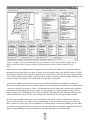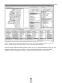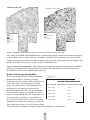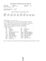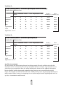
1
Use of Computer and Spatial Technologies
in Large Area Inventories
By
Robert C. Parker, Patrick A. Glass, H. Alexis Londo, David L. Evans,
Keith L. Belli, Thomas G. Matney and Emily B. Schultz
Forest and Wildlife Research Center
Mississippi State University
The Forest and Wildlife Research Center at Mississippi State University was established by the
Mississippi Legislature with the passage of the renewable Natural Resources Research Act of 1994.
The mission of the Center is to conduct research and technical assistance programs relevant to the
efficient management and utilization of the forest, wildlife, and fisheries of the state and region, and
the protection and enhancement of the natural environment associated with these resources. The
FWRC scientists conduct this research in laboratories and forests administered by the University and
cooperating agencies and industries throughout the country. Research results are made available to
potential users through the University’s educational program and through Center publications such
as this, which are directed as appropriate to forest landowners and managers, manufacturers and
users of forest products, leaders of government and industry, the scientific community, and the
general public. Dr. Bob L. Karr is interim director of the Forest and Wildlife Research Center.
Authors
Robert C. Parker and Emily Schultz are associate professors in the Department of Forestry. David L.
Evans, Keith L. Belli, and Thomas G. Matney are professors in the Department of Forestry. H. Alexis
Londo is a Research Associate II in the Department of Forestry. Patrick A. Glass is Director of
Operations for the Mississippi Institute for Forest Inventory.
To Order Copies
Copies of this and other Forest and Wildlife Research Center publications are available from:
Publications Office
Forest and Wildlife Research Center
Box 9680
Mississippi State, MS 39762-9680
Please indicate author(s), title, and publication number if known.
Publications are also available at our web site at www.cfr.msstate.edu.
Citation
Parker, R.C., P.A. Glass, H.A. Londo, D.L. Evans, K.L. Belli, T.G. Matney, E.B. Schultz. 2005.
Mississippi’s forest inventory pilot program: Use of computer and spatial technologies in large area
inventories. Forest and Wildlife Research Center, Bulletin FO 274, Mississippi State University. 43pp.
Research Bulletin FO 274
FOREST AND WILDLIFE RESEARCH CENTER
Mississippi State University
Use of Computer and Spatial Technologies
in Large Area Inventories
By
Robert C. Parker, Patrick A. Glass, H. Alexis Londo, David L. Evans,
Keith L. Belli, Thomas G. Matney and Emily B. Schultz
Forest and Wildlife Research Center
Mississippi State University
The objectives of the Mississippi Forest Inventory Pilot Program were: 1) to develop a forest inventory and information distribution system based on remote sensing, GIS, and GPS technologies in concert with widely accepted
field data collection and computation techniques that can be extended to a statewide system and provide
county-level timber inventory information at a sampling error of +/-10%, and 2) to utilize computer technology
to make original and derived data products available with on-line technologies that will allow users to estimate
timber supplies and monitor forest resource change. Assessment of LandSat™ satellite imagery over successive
time periods facilitated the stratification of forest areas by age class and forest cover type. Other remote sensing
technologies permitted the allocation of truly random plots using stratified random sampling criteria. Allocation
of sample plots was designed to achieve a 10% sampling error at a county level for total cubic volume at the
95% confidence level within the Pilot Program area involving 4 counties of east-central Mississippi. GPS units
coupled to a geostationary satellite were used to navigate on a real-time basis to plot locations with sub-meter
accuracy. Inventory data were recorded on field computers containing specialized software. The satellite image
estimates of forest acreage by age classes of conifers, hardwoods, and mixed conifer-hardwoods were combined
with the inventory data to obtain post-stratified area and volume estimates by tree species, forest cover types,
ownership class, and/or forest origin for user-defined areas with user-accessible Web site software. Procedures
developed in this pilot project can be used in larger land base applications and for integration with and supplementation of existing inventory programs to meet user-defined precision criteria.
Forestry is a leading industry in Mississippi (Munn and Bullard 1997). Data exist for systematic inventory plots
and county summaries (Hartsell and London 1995), but there is no accurate representation of the spatial distribution of timber volume resources. Shifts in timber availability have dramatic impacts on the State’s economy
and environment. Forest change and resource location impact Mississippi’s forest based industries and activities
they support. There is no current system in place to track changes in the spatial distribution of harvesting
(resource depletion) and successful regeneration (future availability; environmental recovery).
The United States Forest Service (USFS) currently conducts Forest Inventory and Analysis (FIA) surveys
(Reams and Van Deusen 1999), which are designed to inventory forest resources nationwide. Historically,
these inventories have been scheduled every 6 to 15 years with a mode of 10 years (Van Deusen 1997).
Inventory plots are distributed systematically throughout a given region. Information computed from these
inventories is designed for large areas (Schreuder and Thomas 1991) and is accurate for assessing the forest
resources of a region or state. The last inventory data available for Mississippi were collected in 1993 and
1994 and included 3190 plots (Reams and Van Deusen 1999). The existing federal data collected were not
1
designed to be statistically precise at the county level. Current inventories also do not describe the distribution of the forests in the state.
The objectives of the Mississippi Forest Inventory Pilot Program were:
1. To develop a forest inventory and information distribution system based on remote sensing, GIS, and GPS
technologies in concert with widely accepted field data collection and computation techniques that can be
extended to a statewide system and provide county-level timber inventory information at a sampling error of
+/-10% at the 95% level of confidence.
2. To make original and derived data products available with on-line technologies that will allow users to
estimate timber supplies and monitor forest resource change.
This research was conducted on a contiguous four-county region in the east-central part of Mississippi and
involved the counties of Choctaw, Clay, Oktibbeha, and Winston (Figure 1).
The pilot study was accomplished through use of LandSat™ (satellite) imagery in conjunction with a field
inventory of forest resources for a multi-county area. Digital classifications of satellite data were used to allocate field sample locations for sampling by project crews and cooperators from the Mississippi Forestry
Commission. All data were incorporated into an Internet World Wide Web site. The primary methods
included:
1. Building a current forest type map for the four-county area of the state.
2. Augmenting the forest type map with ground inventory photo
plots to generate a geospatial database that can be used to determine volume and distribution by timber type and ownership.
3. Making the information developed from objectives one and two
available to the public on an Internet site.
4. Designing a knowledge-based expert system for estimating the
growth of the mapped forest types from existing growth and yield
data and other sources.
5. Designing a system that would combine spatial and resource
data components into a visual online system that would allow the
public to assess forest productivity for any user-defined land area.
2
Figure 1. Four county region for the Forest
Inventory Pilot Program.
Spatial Technologies
Veridian ERIM-International, a contract partner, geo-corrected the LandSat™ data, identified forested areas,
and assessed the age and composition of the areas (Roller 2000). Forest area mapping was based on spectral
categorization of the leaf-on 1998 Thematic Mapper (TM) data. Forest age was assessed using a first and last
date forest stratified, hybrid change detection procedure developed by Veridian ERIM-International. This
procedure yielded six forest age classes based on the available LandSat™ Multispectral Scanner (MSS) and
TM data. Forest composition assessments were based on 1999 leaf-off TM data. The assessment was
performed using a forest and age stratified spectral based procedure. Forest composition was assessed with
respect to the relative amount of evergreen and deciduous forest present within a pixel.
Inventory and Plot Allocation
Sample Size Estimation
The initial estimate of sample size for each of the four counties in the pilot project was determined from
information provided by the 1992 FIA inventory of these counties. The variability calculated for total cubic
foot volume within a county was used to estimate the number of plots needed to meet an allowable
sampling error of ± 10% at the 95% confidence level. The sample size formula for simple random sampling,
rather than the formula for stratified sampling, was used. The former provided a more conservative estimate
given some doubts about applicability of the information gleaned from the FIA database.
The resulting estimates of sample size varied from a high of 98 plots for Choctaw County to a low of 79
plots for Oktibbeha County. Again, based on the conservative approach regarding the preliminary database,
it was decided that 100 plots would be allocated to each county. Plans were also made to follow this initial
allocation with the establishment of additional plots, as necessary, once each county’s volume data were
analyzed. The final plot allocation was 695 plots in the four counties.
Plots were allocated proportionally, based upon area in each cover type, by county. ERDAS Imagine software
was utilized to randomly choose each plot location. In an effort to allow for image geometric correctional
errors and the known capabilities of the Differential Global Positioning Systems (DGPS), the criterior for
choosing these plots was that each must be centered in a homogeneous 180 by 180 m area. Geographic
coordinates projected in Mississippi Transverse Mercator (MSTM) for the center of each area served as plot
centers. These coordinates were re-projected into latitude/longitude and formatted for the DGPS field units.
Field Equipment
GPS Systems
The Corvallis Microtechnology Incorporated (CMT) PC5L GPS™ and the Juniper Systems Landmark GPS™
were utilized to navigate to 695 random plot locations across the four county area (Figure 2). Equipment
failure, either from physical damage to cabling or malfunction, accounted for the largest percentage of
3
reduction in field productivity. Selective Availability, GPS satellite geometry and canopy coverage had
minimal effect on productivity. Field recorder power requirements were comparable providing 10 hours of
intermittent usage without failure. External power supplies for the DGPS decoding system proved to be
bulky and cumbersome. The CMT field delivery system, consisting of a rigid frame backpack, proved more
efficient for transporting the additional inventory equipment than did the flexible backpack of the Juniper
system.
Prior to deactivation of Selective Availability, the rapidity of change in the pseudorange broadcast caused
position fixes calculated by the CMT unit to fluctuate a known point by one to five meters in horizontal
position. When Selective Availability was turned off, the CMT position fixes became more stable, at less than
two meters in horizontal offset. The Juniper system, which displays the position computed within the
Trimble AG 132 receiver, consistently reported positions around a known point within one meter regardless
of Selective Availability influence.
When used under tree canopy conditions, both the CMT and Juniper GPS systems performed best with the
large Trimble dome antenna.
Field Computers
The CMT-PC5L and Juniper Pro4000 field computers (Figure 2) were
used with speciality software (MSINVEN) to record the tree and plot data
and transfer the data to a desktop computer (INVENCOM). The software
was written and compiled with Quick Basic 4.5 and contained assembler
routines for screen handling.
DME Devices
The Haglof Forester DME 201 (Figure 3) was used to measure plot radii
and horizontal distances for tree height measurement. Haglof developed
the DME 201 for use as a distance measuring device in areas where
terrain is uniform. It is a one-handed receiving device that utilizes a
transponder located at plot
center that resonates at 25 kHz
with a 360˚ broadcast area.
Figure 3. Forestor DME 201 (bottom)
with 360° transponders.
Figure 2. Juniper Pro4000 (left)
and CMT-PC5L Field computers
with CMT GPS antenna.
Height Measuring Devices
The Haglof Vertex and Vertex III hypsometers were used for tree
height measurement (Figure 4). They are one-handed receiving
devices that utilize a transponder located on the tree at some
predetermined height, typically breast height, and resonate at 25
kHz with a 60˚ broadcast area to establish baseline distances. Using
the receiver - transponder combination eliminates the need to
measure baselines and the 60˚ broadcast angle for the transponder
allows a wide range of motion for obtaining a clear line of sight.
The ultrasonic equipment demonstrated a high degree of precision
operating through a wide range of environmental conditions.
4
Measurement errors were obvious to operators and could be attributed to either a
depleted power supply or multiple
transponder interference.
DGPS and Navigation Procedures
DGPS allowed the use of stratified random
sampling procedures. After the satellite
imagery was classified and the required
number of plots within each stratum was
allocated, the coordinates for the plots were
organized into navigation files for the DGPS
receivers. Two separate DGPS systems were
Figure 4. Vertex III (left) and Vertex (right) hypsometers.
used for navigation (Figure 5); thus,
requiring translation of the coordinate
information from a standard text format into proprietary formats that the receivers would accept.
Inventory crews utilized image maps generated from the satellite
data and standard topographic maps for navigation to the approximate plot location. Within a range of one mile from the plot
location the crews switched on the DGPS units and utilized the
navigational aids provided by the interface to locate the plot.
Field and Tree Data Collection
To assure consistent and uniform data collection across all
encountered conditions, a procedures manual was developed
(Appendix A). Inventory information was collected in two phases
to allow for a complete description of the forested area. The first
phase observations included the general characteristics of the site
(i.e. slope, stand type, etc.) to ensure the data represented a
homogenous sampling unit. Mensuration data were collected
during the second phase. Measurements were collected for the
Figure 5. CMT and Juniper (left) DGPS
computation of tree volume, inside and outside bark. In addition
field delivery systems.
to stem length being measured to an absolute upper stem diameter limit, stem length was also measured to a usable limit
typifying local mill harvesting practices. Five-and ten-year diameter growth rates were measured to allow
projection for equivalent periods. Site index measurements were recorded to quantify productivity potential.
Portable field computers were used to collect data in an electronic format. This increased the efficiency of
the inventory by eliminating the need for key-punching of the data and the possibility of transcription
errors. Data collection software was developed to accommodate all the information collected and validate
the data entries in real-time (Figure 6). As data were entered into the recorder, they were checked against a
set of values appropriate for that measurement and the user was prompted to verify the entry if the input
value was outside the expected range.
5
Ultrasonic measuring equipment was employed for distance and height measurements to decrease time spent
on the plot. Tree heights were measured with Vertex hypsometers which eliminated the need to establish the
baseline distance required by clinometers. Distance measuring devices, DME 201s, were used to establish plot
radii and to check border trees without pulling a logger’s tape through brush and around obstacles.
a.
d.
b.
c.
e.
f.
Figure 6. Screens from the Pro4000 field computer: a. main menu, b. enter/edit screen for inventory codes, c. full
screen view of tree tally screen, d. window view of tree tally screen, e. plot information screen, and f. sample tree
screen.
Field Training
Training and certification plots were established to represent the possible plot conditions encountered by
field crews conducting the inventory. Training plots demonstrated various conditions that required a qualitative measurement or a subjective decision to be made.
The Mississippi Forestry Commission assigned 13 people to assist with data collection. Junior and senior
level undergraduates from the College of Forest Resources were also employed to collect the field data. Twoperson inventory crews were trained on the certification plots for four consecutive days in order to be certified competent with the equipment and inventory procedures.
Certification procedures required that an inventory crew navigate to and establish an inventory control plot
within specified data collection criteria of time and precision. The inventory data were then printed and the
crew and field supervisor returned to the plot. If there were no errors associated with qualitative or subjective criteria detected, the crew was certified.
6
Verification
Once data collection began, the integrity of the inventory data became the primary priority. Inventory data
were downloaded and screened after each day of collection. It was discovered that the Corvallis MicroTechnology PC5L field computer ram disks were subject to radio frequency interference generated by the
radio units in the Mississippi Forestry Commission vehicles. The impact of this interference ranged from
scrambling some of the data fields to complete erasure of the file allocation table. This necessitated that
these field computers be turned off or located outside a radius of 30 feet during radio transmissions.
Validity of the data was corroborated by check-cruising at a 20% intensity. Specially trained field crews were
assigned check-plots and collected data from these plots as specified by the procedure manual. The two sets
of inventory data were then compared and the original data were considered valid, if discrepancies were
within pre-established limits.
To reduce the total amount of time spent collecting data on a plot, stem lengths were ocularly estimated. To
detect and compensate for any bias in these estimations, the first two trees encountered on a plot were
measured using hypsometers after the ocularly estimated field tally was completed. The corresponding trees
were then paired by individual cruiser and correction curves were developed and applied to the estimated
lengths of all trees on the plot.
Data Format
After collection and verification of the inventory data was completed, the information was organized for the
database. Three separate data files were formed for the database: general stand description information, plot
mensuration data, and growth and site data. These three files were in ASCII format and readily available for
import into a database structure.
An expert system computer algorithm was used to screen the data collected by the field crews and create the
database. The algorithm examined the field data, applied error checking rules set to detect and correct errors,
wrote the corrected data to the database, and printed the original and corrected record for manual correction
of the field data files. This expert system utilized the same external files and settings as did the report generator for complete system compatibility and portability of the error checking facility to any region or scale.
Data Delivery Tools
An interactive dynamic report generator called Mississippi Forest Monitoring and Inventory (MsFMIS)
dynamic report generator was developed to synthesize and deliver information to system users. The software
can derive reports from an inventory database stored on a public server, or optionally on a locally stored
inventory database. It allows the user to select a reporting area on either a county group basis (Figure 7), or
as an irregular polygon (Figure 8). After a report type is selected, the interface presents to the user changes to
match the selected report type. The user can then select the desired stand and tree selection criteria appropriate for the report (species groups, forest types, land ownerships, size classes, products, and others). A beta
version of the program can be downloaded from the Web site www.cfr.msstate.edu. To maintain compatibility with previous FIA databases, and have an interface that is familiar to potential clients, the FIA codes
and names were adopted for the study.
Currently, the MsFMIS produces stand and stock tables, acreage tables, regeneration acreage, and productive
potential stand and stock tabular reports by the selected criteria. Other dynamic link library (dll) report
modules will be added as needed.
7
Figure 7. Example screen from MsFMIS depicting region selection such as county boundaries (upper left) to
define an area from which to generate inventory information based on other criteria indicated by check
boxes.
While the beta version MsFMIS software applies only to the small pilot study area, the program code was
designed to be transportable to any scale or region. All the inventory codes, user interface settings, GIS files,
file locations, and other locale specific settings reside in external files or the system registry. This externalization of locale specific settings allows the program to be adapted to another region by simply modifying the
external settings. No changes in the source code of the program are required.
An interactive Web-based data delivery system was created using the FIA data standards. Developed in
Microsoft Windows® interface format, the data delivery system is designed to provide forest resource data on
a county or regional level (Figures 7 and 8). All information from the field plots is entered into a database
and summarized depending on the user’s needs. Irregular polygons or county boundaries can be used to
define an interest area. Embedded in this system are routines that generate stand and stock tables (per acre
values and totals are given) with the associated precision statistics for the area and volume estimates.
The four report dynamic link libraries to be included with the release version of MsFMIS will allow the
client to derive virtually any volume, acreage, reproduction, or growth estimates showing point and reliability statistics. For report types that are needed on a continuing basis, custom programming will be added
to make the report generation a one-step process. The report generation and database application interfaces
(APIs) will be published so clients can customize the generated reports to suit their needs.
8
Figure 8. Example screen from MsFMIS depicting the selection of an irregular polygon to define an area from
which to generate inventory information based on other criteria indicated by check boxes.
Based on Veridian-ERIM International products, clients can view the spatial distribution of forest age and
composition within the study area (Figure 9). The spatial distributions can be viewed using ESRI’s
ArcExplorer software. ArcExplorer is freeware, and it can be downloaded from www.esri.com.
9
Inventory analysis with MsFMIS was accomplished through an interface that allows the user to define several
criteria for compiling results. The user has the ability to select from several inventory databases. Currently the
USDA-USFS 1992 Southeastern FIA database and the Mississippi Pilot Inventory database are available for
inventory calculations. A unique feature of MsFMIS is the versatility in selecting the area for analysis. An interactive map is provided that allows the selection of a single county or multiple counties, or the selection of a
geographic region by outlining the area of interest with a polygon. The only restriction placed on the regional
selection method is the total area within the polygon must be larger than 200 square miles. This insures that
an adequate number of sample plots are included in the computations. After the region under consideration
has been defined, the user can then expand or restrict the analysis based on the attributes of interest. Four
separate reports will be available with the commercial version (Area, Regeneration, Growth and Volume),
however, the current version only reports timber volumes with standard stand and stock tables.
A typical application scenario for forest industry would be to determine whether an area would be capable
of supporting an additional milling facility. Their analysis objective would be to determine the total volume
available that is capable of meeting milling specifications. Utilizing MsFMIS, the region of interest would be
identified and the generalized criteria: Species, Forest Type, Ownership, Stand Size, Origin, Tree Product,
Logging Operability, Tree and Stand Level Damages and Physiographics would be designated. These selection criteria would then be used to extract and process the inventory information from the database to
produce standardized volume reports. Additionally, MsFMIS computes the associated statistics and sampling
errors for each density and volume category. Particular attention should be paid to the sampling errors associated with the various density and volume estimates. The sampling error presented represents the combined
variance structure from the acreage estimate and the volume estimate.
Imagery-based Products
Forest Cover Mapping – Forest cover maps were produced for the first and last date imagery. Forest cover
mapping was developed using all spectral bands from the MSS and TM imagery. Spectral signatures of forest
cover from the imagery were derived using unsupervised clustering. Maximum likelihood categorization was
used to label the clusters which were based upon phenological image changes and ancillary photogrammetric information.
Forest Age – Forest age was determined using the time sequence of images from initial to most recent dates.
Determination of forest age was performed in two parts: 1) aging of forested land that was detected in the
first year in the sequence of the imagery, and 2) aging of land that had become forested after the first year in
the sequence. Land that was forested in the first year in the sequence and never detected to be harvested
while still being forested in the most recent image was determined to be in the oldest class. Subsequent
classes were aged from the last observed harvest or pre-forested date determined from the intermediate
image dates.
Forest Composition – Forest composition was determined using the two most recent satellite image acquisi-
10
Figure 9. Examples of forest age and composition derived for Choctaw County, Mississippi.
tions. Using the standard normalized difference vegetation index (NDVI) to detect the amount of evergreen
versus deciduous trees in a forested pixel, a continuous variable for all forested pixels was assessed. Using
ancillary photogrametric information and knowledge of the vegetation growth patterns in Mississippi, it was
possible to group the forested areas as pine, mixed, or hardwood forest.
Age and Composition Integration – Integrating forest age and forest composition information resulted in
relating age to composition for any particular forested area. This information was used in assessing the
sustainability of the forested resources in the study area.
Results of Harvesting Sustainability
Table 1.
The average annualized rate of forested harvesting is
summarized in Table 1. An increase in forest
The average annualized rate of forest
harvesting in the early 1980’s and the last half of the
harvesting by observed time interval.
1990’s was evident. This information was based
Time Interval Percent Forest Area Harvested Per Year
upon: 1) the forested area at the beginning of the
0.32
1972-1979
study period, 2) the amount of harvested area
detected throughout the study, and 3) an assumed
0.83
1979-1986
harvest rotation of 40 years (standard at the begin0.17
1986-1992
ning of the study). Based upon this information, the
0.13
1992-1995
forest harvesting is occurring at a sustainable rate
(2.5% per year) in the study area. This is an average
0.88
1995-1998
annualized rate of forest harvesting by area of 0.54%.
These observations relate to clear-tell harvest systems
and do not reflect intermediate thinning during the full rotation of a timber stand.
11
Knowledge-based prototype for estimating growth and yield
A prototype for a knowledge-based growth and yield (KBGY) prediction system was developed to supply
managed stand growth projections and planning and decision support tools for industry, private landowners
and public agencies. The prediction system was constructed in five component modules: 1) MS Windows®
user interface that will be linked to the main MsFMIS interface, 2) a database update facility, 3) the database,
4) search engines and predictive algorithms, and 5) a report writer.
The knowledge-based growth and yield user interface (Figure 10) was implemented in a Visual C++
Figure 10. Example screen from MsFMIS depicting the knowledge-based growth and yield user
interface.
programming environment. The interface includes both required and optional user inputs. The user selects
forest type, stand origin, current and future age, and report type for which growth and yield predictions will
be made. Either current basal area per acre or current trees per acre must also be entered. Site index is an
optional input that, when known, can further refine yield projections. The system assumes, depending on
the type of user, varying degrees of current stand information may be available for input. The more inputs
that are supplied, the more specific the predictions that can be made. For example, if site index is not
entered, predictions will be broadly based across a range of site indices. If site index is supplied, predictions
will be based only on growth and yield plots possessing that site index.
The database update facility was developed as a WIN32 program in Visual C++. This module facilitates the
addition of growth and yield data sets to the database component of the knowledge-based system. As the
database grows, predictions can be made for an increasing number of forest types and management conditions with greater confidence. An ISAM (indexed sequential access method) database structure was utilized
because of its superior access and retrieval speed as compared to relational database structures. It is anticipated that the database component of the full implementation will be extremely large and retrieval time will
be an important issue. Microsoft’s Open Database Connectivity (ODBC) standard for client-side database
access and a standard Structured Query Language (SQL) embedded in Visual C++ code were employed for
writing the database access code necessary to construct the search engine and predictive algorithms.
12
The report writer for the growth and yield system (Figure 11) was designed to display volume information in
a format as similar as possible to the main MsFMIS interface, so as to appear as a seamless link. Volumes are
reported on a per acre basis for inside and outside bark estimates in cubic feet of pulpwood and sawtimber
and for three different board-foot log rules. Depending upon the user selected forest type, volumes are
reported by the associated species group. The current USDA, Forest Service definitions of forest type-species
group associations were utilized. A full implementation of the prototype is expected to be completed within
the next two years. Tasks include the addition of a large number of growth and yield databases, further
refinement of predictive algorithms, and formulation of reliability estimates and their comparison to traditional modeling techniques.
The accuracy assessment of the remote sensing products supplied by Veridian-ERIM International were
completed using the field plot data, historical aerial photographs and current high resolution imagery. The
field plot data and high resolution imagery were used to evaluate the forest cover type products. Historical
aerial photographs were used to assess the age class products. This accuracy assessment was performed by
the Spatial Information Technologies Laboratory of Mississippi State University.
Cover Type Assessments
Overall accuracy, based on the high-resolution aerial imagery, was estimated to be 93.54% (Table 2) while
the accuracy estimated from the field plot evaluations was 64.87% (Table 3). The differences in these figures
can be attributed to how each evaluation was taken. In the field, the assessment is made from under the
canopy, looking up. Assessments from the high resolution imagery are made from above the canopy,
looking down. Another cause for error could be the registration errors between the remote sensing product
and the DGPS. Finally, the errors between the cover types may be a result of the compilation of the five field
plot cover type categories into the three cover type categories produced in the remote sensing products.
13
Figure 11. Example of report generated by MsFMIS from the knowledge based growth and yield user interface.
14
Table 2.
Error matrix assessing LandSat™-derived cover types using high resolution aerial imagery.
Classified Data Reference Data
Non- Hardwood Mixed
Forest
Pine Regeneration Total
Product
User's
Accuracy (%) Accuracy (%)
Non-Forest
56
0
1
0
0
57
83.58
93.33
Hardwood
4
55
0
0
0
59
100.00
93.22
Mixed
0
0
54
0
0
54
98.18
96.49
Pine
0
0
0
58
0
58
100.00
100.00
Regeneration
8
0
0
0
58
66
89.66
86.67
Total
68
55
55
58
58
294
N/A
N/A
Kappa Statistic 0.9193
Table 3.
Error matrix assessing LandSat™-derived cover types using field plot
Classified Data Reference Data
Non- Hardwood Mixed
Forest
Pine Regeneration Total
Product
User's
Accuracy (%) Accuracy (%)
Non-Forest
86
4
18
1
0
109
90.53
78.90
Hardwood
1
95
6
3
1
106
49.48
79.62
Mixed
6
81
173
73
0
333
77.58
51.95
Pine
1
3
12
107
0
123
46.52
86.99
Regeneration
1
9
14
46
56
126
98.25
44.44
Total
95
192
223
230
57
797
N/A
N/A
Kappa Statistic 0.5490
Age Class Assessments
Age class accuracy was assessed using historical aerial photographs. The only available statistic for this
assessment was the overall accuracy for each age class (Table 4). These accuracies range from 90% to 94%.
Again, these were assessed from above the canopy, looking down. Because of the temporal discrepancies
between LandSat™ and the photographs, judgments about stand age were assessed from the original
imagery. For example, if a stand was harvested in the middle of the age class, the photographs would show a
mature stand of timber; however, by comparing the two satellite images from the beginning and end of an
age class, a determination could be made.
15
Table 4.
Accuracies for age classes assessed using historical aerial photographs.
Age Class
Year of Photography
Years Included
(Years)
Accuracy
(%)
0-3
1996-1999
1996
90
4-6
1995-1993
1992
92
7-12
1992-1987
1985
92
13-9
1986-1980
1980
94
20-26
1979-1973
1969
94
+27
Prior to 1973
1969
96
Overall Accuracy
Overall the accuracy of the remote sensing products was within acceptable limits. The difference between
classification techniques using aerial imagery and field data techniques generally show up as differences in
the comparative statistics. As image processing capabilities and the resolution of satellite imagery increase,
these products will be more reliable.
Integration of remote sensing data with GPS technologies is valuable for increasing inventory efficiency and
level of precision. The benefits of this approach are two-fold: first, no effort was expended on sampling nonforested areas and secondly, sampling intensity was matched with the variability of the target resource. This
coupling allowed for a true random sample of forest area by type over a large landscape. Based on the
remote sensing forest typing, precision goals were attained.
Future directions for this product include validation, expansion, and integration with other programs.
Expansion goals are aimed at applications in other states and regions. Finally, the integration of FIA data
will further increase sampling efficiency (Cochran 2002).
16
Cochran, J. K. 2002. County level inventories - can FIA help? Thesis, Department of Forestry, Mississippi
State University.
Hartsell, A., and J. London. 1995. Forest statistics for Mississippi counties - 1994. USDA, Forest Service, So.
For. Exp. Stn. Res. Bull. SO-190. 89 p.
Munn, I. A., and S. H. Bullard. 1997. Pulp and paper industries — multi-billion dollar contributions to
Mississippi’s economy. Tree Talk 19(2):12-13.
Roller, N. 2000. Intermediate multispectral satellite sensors. J. For. 98(6):32-35.
Reams G. A, and P. C. Van Deusen. 1999. The southern annual forest inventory system. J. of Ag. Bio. and
Envir. Stat. 4(4):346-360.
Schreuder, H. T., and C. E. Thomas. 1991. Establishing cause-effect relationships using forest survey data.
For. Sci. 37(6):1497-1512.
Van Deusen, P. C. 1997. Annual forest inventory statistical concepts with emphasis on multiple imputation.
Can. J. For. Res. 27:379-384.
17
18
Pilot Program for a Forest Monitoring
and Information System
Field Procedures
Manual
Volume 1
written by:
Patrick A. Glass
Revised October 21, 1999
Pilot Program for a Forest Monitoring and Information System
Measurement Plot Specifications and Procedures . . . . . . . . . . . . . . . . . . . . . . . . . . . . . . . . . . . . . . . . . . . . . . . . .1
Field Crews . . . . . . . . . . . . . . . . . . . . . . . . . . . . . . . . . . . . . . . . . . . . . . . . . . . . . . . . . . . . . . . . . . . . . . . . . . . . . . . .1
Field Equipment . . . . . . . . . . . . . . . . . . . . . . . . . . . . . . . . . . . . . . . . . . . . . . . . . . . . . . . . . . . . . . . . . . . . . . . . . . . .1
Land Navigation . . . . . . . . . . . . . . . . . . . . . . . . . . . . . . . . . . . . . . . . . . . . . . . . . . . . . . . . . . . . . . . . . . . . . . . . . . . .2
Equipment Calibration . . . . . . . . . . . . . . . . . . . . . . . . . . . . . . . . . . . . . . . . . . . . . . . . . . . . . . . . . . . . . . . . . . . . . . .2
Plot Establishment . . . . . . . . . . . . . . . . . . . . . . . . . . . . . . . . . . . . . . . . . . . . . . . . . . . . . . . . . . . . . . . . . . . . . . . . . .2
Plot Description . . . . . . . . . . . . . . . . . . . . . . . . . . . . . . . . . . . . . . . . . . . . . . . . . . . . . . . . . . . . . . . . . . . . . . . . . . . .3
Slope . . . . . . . . . . . . . . . . . . . . . . . . . . . . . . . . . . . . . . . . . . . . . . . . . . . . . . . . . . . . . . . . . . . . . . . . . . . . . . . . .3
Stand Condition . . . . . . . . . . . . . . . . . . . . . . . . . . . . . . . . . . . . . . . . . . . . . . . . . . . . . . . . . . . . . . . . . . . . . . . . .3
Size Class . . . . . . . . . . . . . . . . . . . . . . . . . . . . . . . . . . . . . . . . . . . . . . . . . . . . . . . . . . . . . . . . . . . . . . . . . . . . . . .3
Origin . . . . . . . . . . . . . . . . . . . . . . . . . . . . . . . . . . . . . . . . . . . . . . . . . . . . . . . . . . . . . . . . . . . . . . . . . . . . . . . . .4
SAT Code . . . . . . . . . . . . . . . . . . . . . . . . . . . . . . . . . . . . . . . . . . . . . . . . . . . . . . . . . . . . . . . . . . . . . . . . . . . . . . .4
SAF Cover-Type . . . . . . . . . . . . . . . . . . . . . . . . . . . . . . . . . . . . . . . . . . . . . . . . . . . . . . . . . . . . . . . . . . . . . . . . . .5
Ownership . . . . . . . . . . . . . . . . . . . . . . . . . . . . . . . . . . . . . . . . . . . . . . . . . . . . . . . . . . . . . . . . . . . . . . . . . . . . . .5
Physiographic Position . . . . . . . . . . . . . . . . . . . . . . . . . . . . . . . . . . . . . . . . . . . . . . . . . . . . . . . . . . . . . . . . . . . .5
Logging Operability . . . . . . . . . . . . . . . . . . . . . . . . . . . . . . . . . . . . . . . . . . . . . . . . . . . . . . . . . . . . . . . . . . . . . .6
Latitude / Longitude . . . . . . . . . . . . . . . . . . . . . . . . . . . . . . . . . . . . . . . . . . . . . . . . . . . . . . . . . . . . . . . . . . . . . .6
Plot Measurements . . . . . . . . . . . . . . . . . . . . . . . . . . . . . . . . . . . . . . . . . . . . . . . . . . . . . . . . . . . . . . . . . . . . . . . . . .6
Individual Tree Tally . . . . . . . . . . . . . . . . . . . . . . . . . . . . . . . . . . . . . . . . . . . . . . . . . . . . . . . . . . . . . . . . . . . . . . . . .7
Plot
. . . . . . . . . . . . . . . . . . . . . . . . . . . . . . . . . . . . . . . . . . . . . . . . . . . . . . . . . . . . . . . . . . . . . . . . . . . . . . . . .7
Product . . . . . . . . . . . . . . . . . . . . . . . . . . . . . . . . . . . . . . . . . . . . . . . . . . . . . . . . . . . . . . . . . . . . . . . . . . . . . . . .7
Species . . . . . . . . . . . . . . . . . . . . . . . . . . . . . . . . . . . . . . . . . . . . . . . . . . . . . . . . . . . . . . . . . . . . . . . . . . . . . . . . .7
Diameter . . . . . . . . . . . . . . . . . . . . . . . . . . . . . . . . . . . . . . . . . . . . . . . . . . . . . . . . . . . . . . . . . . . . . . . . . . . . . . .8
Total Height . . . . . . . . . . . . . . . . . . . . . . . . . . . . . . . . . . . . . . . . . . . . . . . . . . . . . . . . . . . . . . . . . . . . . . . . . . . . .8
Pulpwood Height to Absolute Top . . . . . . . . . . . . . . . . . . . . . . . . . . . . . . . . . . . . . . . . . . . . . . . . . . . . . . . . . .8
Pulpwood Usable Height . . . . . . . . . . . . . . . . . . . . . . . . . . . . . . . . . . . . . . . . . . . . . . . . . . . . . . . . . . . . . . . . . .8
Saw timber Height to Absolute Top . . . . . . . . . . . . . . . . . . . . . . . . . . . . . . . . . . . . . . . . . . . . . . . . . . . . . . . . .8
Saw timber Usable Height . . . . . . . . . . . . . . . . . . . . . . . . . . . . . . . . . . . . . . . . . . . . . . . . . . . . . . . . . . . . . . . . .8
Damage . . . . . . . . . . . . . . . . . . . . . . . . . . . . . . . . . . . . . . . . . . . . . . . . . . . . . . . . . . . . . . . . . . . . . . . . . . . . . . . .8
Broken Top . . . . . . . . . . . . . . . . . . . . . . . . . . . . . . . . . . . . . . . . . . . . . . . . . . . . . . . . . . . . . . . . . . . . . . . . . . . . .9
Field Procedures . . . . . . . . . . . . . . . . . . . . . . . . . . . . . . . . . . . . . . . . . . . . . . . . . . . . . . . . . . . . . . . . . . . . . . . . . . . .9
Height Sub-Sample . . . . . . . . . . . . . . . . . . . . . . . . . . . . . . . . . . . . . . . . . . . . . . . . . . . . . . . . . . . . . . . . . . . . . . . . .10
Growth Projection Measurements . . . . . . . . . . . . . . . . . . . . . . . . . . . . . . . . . . . . . . . . . . . . . . . . . . . . . . . . . . . . .11
Site Index Measurements . . . . . . . . . . . . . . . . . . . . . . . . . . . . . . . . . . . . . . . . . . . . . . . . . . . . . . . . . . . . . . . . . . . .11
Plot Exit
. . . . . . . . . . . . . . . . . . . . . . . . . . . . . . . . . . . . . . . . . . . . . . . . . . . . . . . . . . . . . . . . . . . . . . . . . . . . . . . .11
Appendix 1 . . . . . . . . . . . . . . . . . . . . . . . . . . . . . . . . . . . . . . . . . . . . . . . . . . . . . . . . . . . . . . . . . . . . . . . . . . . . . . .12
Common Name - Species Reference . . . . . . . . . . . . . . . . . . . . . . . . . . . . . . . . . . . . . . . . . . . . . . . . . . . . . . . .12
Appendix 2 . . . . . . . . . . . . . . . . . . . . . . . . . . . . . . . . . . . . . . . . . . . . . . . . . . . . . . . . . . . . . . . . . . . . . . . . . . . . . . .14
SAF Cover Type Definitions . . . . . . . . . . . . . . . . . . . . . . . . . . . . . . . . . . . . . . . . . . . . . . . . . . . . . . . . . . . . . . .14
Appendix 3 . . . . . . . . . . . . . . . . . . . . . . . . . . . . . . . . . . . . . . . . . . . . . . . . . . . . . . . . . . . . . . . . . . . . . . . . . . . . . . .16
Power Supply . . . . . . . . . . . . . . . . . . . . . . . . . . . . . . . . . . . . . . . . . . . . . . . . . . . . . . . . . . . . . . . . . . . . . . . . . .16
G.P.S. . . . . . . . . . . . . . . . . . . . . . . . . . . . . . . . . . . . . . . . . . . . . . . . . . . . . . . . . . . . . . . . . . . . . . . . . . . . . . .16
Hypsometer . . . . . . . . . . . . . . . . . . . . . . . . . . . . . . . . . . . . . . . . . . . . . . . . . . . . . . . . . . . . . . . . . . . . . . . .16
DME 201 . . . . . . . . . . . . . . . . . . . . . . . . . . . . . . . . . . . . . . . . . . . . . . . . . . . . . . . . . . . . . . . . . . . . . . . . . . .16
Appendix 4 . . . . . . . . . . . . . . . . . . . . . . . . . . . . . . . . . . . . . . . . . . . . . . . . . . . . . . . . . . . . . . . . . . . . . . . . . . . . . . .17
Transponder Activation . . . . . . . . . . . . . . . . . . . . . . . . . . . . . . . . . . . . . . . . . . . . . . . . . . . . . . . . . . . . . . . . . .17
Appendix 5 . . . . . . . . . . . . . . . . . . . . . . . . . . . . . . . . . . . . . . . . . . . . . . . . . . . . . . . . . . . . . . . . . . . . . . . . . . . . . . .18
Calibration . . . . . . . . . . . . . . . . . . . . . . . . . . . . . . . . . . . . . . . . . . . . . . . . . . . . . . . . . . . . . . . . . . . . . . . . . . . .18
Hypsometer . . . . . . . . . . . . . . . . . . . . . . . . . . . . . . . . . . . . . . . . . . . . . . . . . . . . . . . . . . . . . . . . . . . . . . . .18
DME 201 . . . . . . . . . . . . . . . . . . . . . . . . . . . . . . . . . . . . . . . . . . . . . . . . . . . . . . . . . . . . . . . . . . . . . . . . . . .18
Appendix 6 . . . . . . . . . . . . . . . . . . . . . . . . . . . . . . . . . . . . . . . . . . . . . . . . . . . . . . . . . . . . . . . . . . . . . . . . . . . . . . .19
Auxiliary CMT Operations . . . . . . . . . . . . . . . . . . . . . . . . . . . . . . . . . . . . . . . . . . . . . . . . . . . . . . . . . . . . . . . .19
Screen Contrast . . . . . . . . . . . . . . . . . . . . . . . . . . . . . . . . . . . . . . . . . . . . . . . . . . . . . . . . . . . . . . . . . . . . . .19
Power Supply . . . . . . . . . . . . . . . . . . . . . . . . . . . . . . . . . . . . . . . . . . . . . . . . . . . . . . . . . . . . . . . . . . . . . . .19
Appendix 7 . . . . . . . . . . . . . . . . . . . . . . . . . . . . . . . . . . . . . . . . . . . . . . . . . . . . . . . . . . . . . . . . . . . . . . . . . . . . . . .20
Slope Determination . . . . . . . . . . . . . . . . . . . . . . . . . . . . . . . . . . . . . . . . . . . . . . . . . . . . . . . . . . . . . . . . . . . .20
Appendix 8 . . . . . . . . . . . . . . . . . . . . . . . . . . . . . . . . . . . . . . . . . . . . . . . . . . . . . . . . . . . . . . . . . . . . . . . . . . . . . . . .21
Data Recording Sheets . . . . . . . . . . . . . . . . . . . . . . . . . . . . . . . . . . . . . . . . . . . . . . . . . . . . . . . . . . . . . . . . . . .21
Measurement Plot Specifications and Procedures
This document supplies definitions, methodologies and standards for the inventory implementation of a
pilot program for a forest monitoring and information system. The objective of this document is to describe
field procedures that will assure consistent and uniform data collection over all expected conditions in the
study area. It is expected that all plot data can be measured by a two-person crew in approximately two
hours, on average, including time spent traversing to and from the plot.
Field Crews:
Each field crew will consist of two individuals. Each individual will be assigned a file designator. The file
designator identifies, within the data structure, which person conducted the height estimations.
To reduce bias of ocular estimations, the same individual will perform estimations throughout the day. Prior
to leaving the office, determine which crew member will perform height estimations. Upon commencement
of plot measurements, the same individual will complete all height estimations for that plot.
Field Equipment:
Each field crew will be assigned a complete set of field equipment. In addition to equipment, a backup
system (compass, clipboard, field data sheets and note pads) will be accessible to prevent loss of time due to
equipment failure.
A G.P.S. receiver will be used to navigate to plot locations, and a field recorder will be utilized to record
inventory data.
Tree heights will be measured with a Vertex hypsometer. The data will be used to obtain local volume tables
and site index estimations on a subsample of trees on each plot. Hypsometers will also be used to obtain a
measurement of slope for each plot.
DME 201 units will be used to check radial distances for boundary trees. Because of the nested plot design
and diameter limited plot radii, each tree’s radial distance will be verified.
Two increment borers (12 inch and 18 inch) will be issued to each crew. The 18 inch borer will be held in
reserve for large trees. The borers will be used to obtain 5 and 10 year radial growth and age at breast height
for site index. A bark gauge will be used to determine single bark thickness.
Logger’s tapes will be supplied for diameter at breast height (d.b.h.) measurements. They will also be used
to measure distances in the event the DME 201’s or the hypsometers fail.
Clinometers will be carried as a precaution against equipment failure. Spare batteries for the hypsometer
and the DME 201 will be carried to prevent delays caused by depleted power sources.
It is the responsibility of each field crew to maintain the equipment. In the event equipment is lost or
becomes non-serviceable, the field coordinator should be notified as soon as possible.
1
Land Navigation:
Each plot location has been randomly selected from remote sensing information to fulfill accuracy requirements for the strata it represents. Latitude and longitude coordinates are used to identify plot centers. Gross
navigation to each plot is achieved using available maps depicting vehicular access routes. It is extremely
unlikely that plot access will be available to motor vehicles. If permission from the landowner can be
obtained prior to site visitation it may be possible to minimize the amount of time spent traversing to the
plot location.
At no time will a field crew be authorized to tamper with, vandalize or destroy fencing or gates defining
property boundaries to facilitate access. Damage or destruction of property with the intent to aid navigation
is not permitted. In the event of long traverses trail marking to assist with egress is restricted to flagging the
line of travel, provided flagging is biodegradable and not used excessively.
Equipment Calibration:
The Vertex hypsometer and the DME 201 require calibration with ambient environmental conditions to
compute distances accurately. Calibration will be conducted each time a field crew exits the vehicle in route
to a new plot location. The procedures for calibrating each instrument are included in Appendix 5. Because
both instruments can utilize either transponder it is more efficient to calibrate both instruments together.
The stipulation with calibration is that the unit has time to adjust to ambient temperature and humidity
conditions before calibrating. This is pertinent whenever the unit is initialized at the beginning of the day or
has been in a vehicle for extended periods of time. Allow the units to adjust to environmental conditions for
10 minutes before calibration.
Plot Establishment:
The first determination to be made upon arrival at plot center is whether the plot will encompass a homogenous sampling unit. If there is no significant variation in type, size or age class, then plot center is
established at the point navigated to with the GPS unit. If significant variation is encountered the plot center
must be moved 1 chain from the original plot center, perpendicular to the stand line, into the stand occupying a majority of the plot. Micro-pockets (less than 10 acres) within a contiguous stand are considered to
be part of the surrounding stand.
Examples where plot locations should be moved:
1) A plot overlaps the type boundary of a plantation and natural pine stand. The plot should be moved
into the natural stand.
2) A plot overlaps the boundary of a thinned and unthinned stand. The plot should be moved into the
unthinned stand.
3) A plot overlaps the boundary of a seed-tree and clear cut stand. The plot should be moved into the seedtree stand.
4) A plot overlaps the boundary of a pine and mixed pine-hardwood stand. The plot should be moved into
the mixed pine-hardwood stand.
5) A plot includes area converted to a non-forestry application (e.g. agriculture, roads, etc.).
2
Inaccessibility of plot center is not a reason for re-positioning. Plot locations may fall within or include
watercourses or natural catchments. If the plot cannot be established without jeopardizing the safety of the
crew, then a notation must be made and the field supervisor notified.
Plot Description:
Each plot sampled will be identified with a unique number. The plot number will index all data entered
into the field recorder. In addition to plot number, descriptive information for each plot will be entered.
Slope, Size Class, Origin, SAF Type, Ownership, Physiographic Position, Logging Operability and Stand
Condition will be catalogued within each plot.
Slope - Identifies the average slope for the plot.
Slope observations are made with the hypsometer on a line parallel to the slope. Procedures for
obtaining slope measurements are detailed in Appendix 7.
Stand Condition - Describes the current condition of the stand with respect to damage and harvesting activities. Explicit codes are defined in table 1.
Table 1.
Stand level damage categories, descriptions and data code.
Damage Type Description
Undamaged
Insect
Disease
Fusiform
Fire
Storm
Ice
Salvage
Thinning
Clear-cut
Seed Tree
Code
There is no apparent damage within the stand.
Infestation of the stand as evidenced by pitch tubes, bore holes, webbed foliage, etc.
Infection of the stand as evidenced by brooming, cankers, conks, etc.
Infection of the stand by Cronartium fusiforme.
Damage to the boles and/or lower canopy from heat
(excluding typical damage from prescribed burns).
Damage by excessive winds from hurricanes or tornadoes is prevalent
(blowdown / windthrow).
Damage to the upper stems and crowns caused by ice accumulation
(breakage in upper crown).
Focused harvesting operations have occurred within the stand.
Generalized harvesting has occurred throughout the stand.
The stand has recently been harvested and no routinely used method of
regeneration is apparent.
The stand has recently been harvested and seed trees for regeneration are present.
1
2
3
4
5
6
7
8
9
10
11
Size Class - Classifies the merchantability class for the plot based on overall size composition. The predominate size class encountered on the plot defines the size class. Table 2 lists acceptable size class designations.
3
Table 2.
Plot merchantability classes, class description and data code for plot size class.
Size Class
Class Description
Reproduction
Sub-Merchantable
Pulpwood
Saw timber
Non Timber
No commercial tree species greater than 1 inch in d.b.h. are encountered
within the radius of a 1/5th acre plot (excludes seed tree stands).
No commercial tree species greater than 4.5 inches in d.b.h. are encountered
within the radius of a 1/5th acre plot.
The majority of commercial tree species occupying the 1/5th acre plot
are 4.6 to 10.6 inches in d.b.h.
The majority of commercial tree species occupying the 1/5th acre plot
are greater than 10.6 inches in d.b.h.
The site has been converted to a non-forestry application.
Code
1
2
3
4
5
Origin - Identifies the origin of the stand. Table 3 identifies acceptable origin codes.
Table 3.
Origin (regeneration method) categories, category description and data codes.
Origin
Description
Code
Natural
Planted
Undetermined
Regeneration occurred from natural processes.
Regeneration occurred from planted stock.
Regeneration method is not readily apparent.
1
2
3
SAT Code - Identifies the canopy coverage in a broader perspective than the SAF cover type. Table 4 provides
guidelines for defining SAT codes.
Table 4.
SAT categories, category description and data codes.
SAT Codes
Description
Code
Pine
Pine Hdwd
Mixed
Hdwd Pine
Hdwd
Canopy composition is greater than 80% coniferous.
Canopy composition is between 60% and 80% coniferous.
Canopy composition is between 40% and 60% coniferous.
Canopy composition is between 20% and 40% coniferous.
Canopy composition is less than 20% coniferous.
4
1
2
3
4
5
SAF Cover-Type - Identifies the canopy species composition using SAF accepted cover types. There are 35
separate cover types that can be encountered. For the inventory, the definitive guide is “Forest Cover
Types of the United States and Canada” published by the SAF (1980). Abbreviated descriptions are
included with the code designations in Appendix 2.
Ownership - Identifies the primary ownership entity. Identification of ownership is not paramount to
performance of the inventory. Minimal time should be spent discerning this variable. If ownership is
obvious then identification should be made. Table 5 depicts the 10 categories that will describe all
ownership possibilities.
Table 5.
Land ownership categories, category description and data codes.
Ownership
Description
Private Non-Industrial
Industrial
USFS
USFWS
Other Fed
State Gov
Municipal
Urban
Tribal
Unknown
Code
Acreage that does not appear to be intensively managed for forestry.
Acreage that has the appearance of intensive management for forestry.
Acreage that is owned or operated by the USDA Forest Service.
Acreage that is owned or operated by the USDI Fish and Wildlife Service.
Acreage that is owned or operated by any other federal entity including BLM,
National Park Service, etc.
Acreage that is owned or operated by the State, including state parks,
16th section land, etc.
Acreage that is owned or operated by municipalities including city parks,
public golf courses, etc.
Acreage that is owned or dwelled upon for residential purposes including
subdivisions, private golf courses, etc.
Acreage that is owned or operated by federally recognized Native
American tribes including Choctaw, Chickasaw, etc.
Acreage that ownership cannot be readily identified.
1
2
3
4
5
6
7
8
9
10
Physiographic Position - Classifies the geographic position of the plot. Table 6 supplies descriptions that will
define relative position. Strict definitions are not applicable to identify physiographic position because
of the variability experienced state wide.
Table 6.
Topographic position categories, category description and data codes.
Physiography
Description
Code
Upland
Bottom
Terrace
Drier, xeric sites found on top of ridges and side slopes.
Wet, hydric sites found along rivers and streams.
Mesic sites that by default are not upland or bottom.
5
1
2
3
Logging Operability - Classifies the terrain for season and equipment accessibility. Table 7 lists the applicable designators for logging operability.
Table 7.
Logging operability categories, category description and data code.
Logging Operability
Description
Code
Year Round
Summer/Fall
Crawler
High Lead
Inoperable
Accessible to logging equipment throughout the calendar year.
Accessible to logging equipment during these seasons only.
Soil or slope precludes the use of rubber tired skidders.
Cable harvesting systems are required.
Cannot be harvested economically or efficiently.
1
2
3
4
5
Latitude / Longitude - Identifies the plot center location in the event that location was moved from the
preset.Before exiting the GPS software make a notation of the new corrected Latitude/Longitude of plot
center. The new coordinates must be entered into these fields, if the plot center was moved from the
preset navigation point.
Plot Measurements:
Three concentric overlapping plot sizes are incorporated within each plot. A 1/5th (0.20) acre plot with
a radius of 52.7 feet is utilized to sample
merchantable timber (4.6 inches in d.b.h. and
larger). A 1/20th (0.05) acre plot with a radius of
26.3 feet is used to inventory sub-merchantable
trees between 1 and 4.5 inches in d.b.h. A 1/100th
(0.01) acre plot with a radius of 11.8 feet is used to
record regeneration 0.0 to 1 inch in d.b.h. Refer to
figure 1 for a representation of the plot design. Two
sweeps will be made around the plot. One sweep is
made for merchantable and sub-merchantable
stems. The other sweep is made within the regeneration plot. Regeneration plots are only established
on locations where the “Size Class” is designated
“Reproduction.” Sweeps will start on the radial line
with a north azimuth to ensure there are no duplicate tallies.
1/100th acre plot radius
1/20th acre plot radius
1/5th acre plot radius
Figure 1. Plot layout depicting effective radii.
6
Individual Tree Tally:
Each live tree will have the following observations recorded. Product, species, d.b.h., total height, pulpwood
height to an absolute top, usable pulpwood height, saw timber height to an absolute top, usable saw timber
height, apparent damage and broken top diameterob if present.
Plot: The unique number assigned to this particular set of Latitude / Longitude coordinates.
Product: A numeric code that describes the primary merchantability of the stem. Table 8 defines the specifications for the product classes.
Table 8.
Product merchantability categories, category description and data code.
Product Category
Description
Reproduction
All commercial species that are less than 1.0 inch d.b.h.
These trees are tallied according to height class.
Commercial species less than 1 foot in height.
Commercial species between 1 and 3 feet in height.
Commercial species greater than 3 feet in height.
All commercial species that are between 1 and 4.5 inches d.b.h.
Total height for these trees is estimated to the nearest foot.
All commercial species that are 4.6 inches d.b.h. or greater that do not
meet the qualifications for a product of greater value.
Pine species that are 7.6 inches d.b.h. or greater and broadleaf species that are
11.6 inches d.b.h. or greater and of sufficient quality to be utilized as saw timber.
Trees that are 15.6 inches d.b.h. or greater and have 16 feet of clear butt log.
Trees that are 11.6 inches d.b.h. or greater free of defect and sweep. Restricted to
pine species (longleaf and slash) predominately found in southern coastal plain.
Hardwood species (red and white oaks) that are not suitable for saw timber
but higher quality than pulpwood.
Any tree that has obvious defects that preclude its inclusion in any of the other
product classifications (i.e. large areas of decay, very poor form, etc.)
The first two non-cull trees (merchantable and/or sub-merchantable) tallied on
each plot are carefully measured for all pertinent heights. This sample is taken after
the reproduction plot information is recorded. Heights are measured by the same
individual that estimated heights.
Class 1
Class 2
Class 3
Sub-merchantable
Pulpwood
Saw Timber
Peeler
Pole
Railroad Tie
Cull
Height Sample
Code
1
2
3
4
5
6
7
8
9
Species: A numeric code from 1 - 60 that identifies the species of the tree. The predominant commercial
species are assigned a code to be input. Additionally, genus codes are supplied in the event that species
identification is not possible. Appendix 1 supplies the code, common name and species name.
7
Diameter: The diameter of the stem, at breast height, in tenths of an inch. Diameter is measured at 4.5 feet
above ground level on the uphill side of the stem. If there is a deformity at d.b.h. then diameter is
preferably measured 1 foot above the point where the stem resumes normal growth. If this point is inaccessible then the diameter is measured 1 foot below the point where the abnormality occurs. If the stem
forks (visible separation) below d.b.h. then each of the multiple stems are treated as separate trees and
measurements are taken at d.b.h. If the stem (visible separation) forks at or above d.b.h. then the stem is
treated as a single tree and the diameter is taken at the base of the fissure scar. If the tree exhibits excessive butt swell as usually encountered with cypress and gum species then the diameter is measured 1
foot above the point where the stem resumes normal form. Parasitic vegetation (clinging vines, etc.)
should be removed to assure that only the tree diameter is measured.
Total Height: The height of the tree (nearest foot) to meristematic tip or uppermost leader. Most conifers
will exhibit one stem terminating with an apical meristem. If the main stem is intact, then height is
measured to the apical tip of the tree. If the main stem has been damaged, then height is measured to
the point where the breakage occurs. Broadleaf trees typically do not possess a single upper stem. They
will however usually have a dominant leader. If a dominant leader can be identified then height is measured to its tip. If the top has been broken out then height is measured to the point of breakage on the
largest diameter limb.
Pulpwood Height to Absolute Top: For conifer species, the height where the main stem is 3 inches DOB; for
broadleaf species, the height where the main stem or largest diameter limb is 4 inches DOB (nearest
foot). This height is recorded for both pulpwood and saw timber trees
Pulpwood Usable Height: The height at which the stem becomes un-usable in typical industry applications.
This height will always be less than or equal to the height to an absolute top (nearest foot). This height
is also recorded for both pulpwood and saw timber trees. Examples of usability limits are given below.
1) The stem forks at 5 inches DOB.
2) The stem forks and none of the multiple stems are 5 inches DOB.
3) The stem is broken.
4) The stem has crook and there is not 5.5 feet of stem pulpwood above the crook.
Saw timber Height to Absolute Top: For conifer species, the height where the main stem is 6 inches DOB;
for broadleaf species, the height where the main stem is 10 inches DOB (nearest foot).
Saw timber Usable Height: The height at which the stem becomes un-usable in typical industry application.
This height will always be less than or equal to height to an absolute top (nearest foot). Examples of
usability limits are given below.
1) The stem forks and none of the multiple stems meet minimum saw timber diameter.
2) The stem incurs crook.
3) The stem is broken.
4) There is a branch whorl of 3 or more branches.
5) A branch is less than 45 degrees off vertical and is one-third the stem diameter where it branches.
6) A branch is equal to one-half the stem diameter.
Damage: Table 9 provides damage categories that will be used to relate tree level damage assessments.
8
Table 9.
Tree level damage categories, descriptions and data code.
Damage Type
Description
Undamaged
Insect
Disease
Fusiform
Fire
Storm
Ice
Mechanical
Decay
Lightning
Erosion
Code
The tree displays no apparent damage.
Infestation of the tree as evidenced by pitch tubes, bore holes, webbed foliage, etc.
Infection of the tree as evidenced by brooming, cankers, conks, etc.
Infection of the tree by Cronartium Fusiforme.
Damage to the bole and/or lower canopy from heat (excluding typical damage
from prescribed burns).
Damage by excessive winds from hurricanes or tornadoes is prevalent
(blowdown / windthrow).
Damage to the upper stem and crown caused by ice accumulation
(breakage in upper crown).
Damage caused by human activity.
Decay of portions of the tree due to exposure.
Direct strikes evidenced by spiraling scars on the stem.
Exposure of root system by flowing water or wind removal of soil.
1
2
3
4
5
6
7
12
13
14
15
Broken Top: The stem diameterob where the break occurs. For broadleaf species this is defined where the
largest diameter stem has been broken.
Field Procedures:
Upon exiting the vehicle turn the G.P.S. unit on, enter G.P.S. software if not resident, by typing “GPS” at the
prompt. Select Navigation from the main menu and allow the unit to initialize. During the time of initialization the hypsometer and DME 201’s will be calibrated. After initialization, the primary navigation screen
will appear. Select the route containing the plot locations, then select the way point (plot) to be sampled.
The unit will then show the azimuth and range to the plot location from your current position.
A directional aid is displayed on the navigation screen in the form of an arrow inside a circle, next to a fixed
arrow orientated with the top of the screen. When the two arrows are parallel the unit is oriented in the
direction of the plot. Proceed in the direction indicated; the unit is set to sound a proximity alarm and
display a message when within 10 feet of plot center. Utilizing the range indicator, minimize the distance to
the plot center.
Temporarily mark the plot center and assess for homogeneity of forest characteristics. If the plot can be
established at that point then exit the G.P.S. software by pressing esc until questioned for confirmation of
exit. Press F5 to confirm exit.
If the plot has to be moved, make the necessary determination for direction and move the plot. When the
9
plot center is established to contain homogenous stand conditions, escape (esc) to the main menu in the
G.P.S. software. Scroll to the Collect Data menu item and press enter. Press F3 to access the base data and
when prompted for a file name press return. After a few seconds the base location data screen will appear.
From this screen note the latitude and longitude for the new plot center. It will be input during the plot
inventory. Press esc until returned to the main menu and then exit the G.P.S. software.
Start the field recording software by typing “PLOT” at the prompt and pressing the enter key. Select menu
item 3 to start recording inventory data. When asked for job name enter your file designator (FML01). When
asked about previous specs press ‘y’ followed by enter. Enter the plot number and press enter. Press the F3
key to access the “PLOT INFORMATION” screen. Press ‘N’ followed with enter. Input the appropriate data
into the various fields as required. Remember to record new plot location coordinates, if plot center was
moved. When all data have been entered for plot description then press F4 to return to the individual tree
tally screen.
Starting from the radial line with a north azimuth, proceed in a clockwise direction, to record merchantable
and sub-merchantable tree data. The first two trees tallied are to be nondestructively marked for subsequent
height measurements. Borderline trees are to be tallied if the distance from the center of the stem to plot
center is less than or equal to plot limiting distance. Classify the tree into the highest product category for
which it qualifies. Identify the species of the tree if possible. If species identification is not possible, or the
species is not included in the species list, then use the general codes (1, 8, 16, 58, 59) to identify the tree. If
genus identification is not possible then classify the species as unknown. Measure the diameter of the tree to
the nearest tenth of an inch. If the tree qualifies as pulpwood, then estimate the total height, absolute
merchantable pulpwood height and usable pulpwood height. If a tree qualifies as saw timber (Peelers, Poles
and Railroad Ties are considered saw timber for height measurements), then estimate total height, absolute
merchantable pulpwood height, usable pulpwood height, absolute merchantable saw timber height and
usable saw timber height. If the tree is sub-merchantable, measure diameter and estimate total height. If the
tree is a cull, then measure diameter only.
Perform an inventory of reproductive material only on plots for which the size class is designated as reproduction, after all merchantable and sub-merchantable stems have been tallied. Reproduction size classes are
entered into the TH field and the number of trees for that species/size class combination are entered into
the PHa field. If there are more than 20 individuals encountered for any species/size class combination then
enter 20 and proceed with the next combination.
Height Sub-Sample:
The first two trees that were tallied and marked are measured with the hypsometer for total, absolute and
usable heights. The measurements are to made by the same individual that estimated the heights. Deactivate the DME 201 transponder by removing it from the range pole. Activate the hypsometer transponder
by swiveling the pins outward from the casing. After measuring d.b.h. attach the transponder to the tree at
d.b.h. Move away from the tree in a direction that will allow the clearest line of sight for as much of the tree
as possible. Distance from the tree should allow for less than a 45˚ angle from the horizontal when sighting
the top of the tree (i.e. distance equal to the height of the tree). Sight the transponder with the hypsometer
until the targeting dot disappears. Then sight the top of the tree until the targeting dot disappears. Continue
10
to sight additional heights as necessary until all height measurements obtainable from that tree are
complete. Repeat the process for the second tree. Under no circumstances are height subsample measurements performed prior to height estimations for the plot tally.
Growth Projection Measurements:
Three merchantable and one sub-merchantable tree will be sampled for growth at each plot. The dominant
species occupying the plot will determine the species of the sample trees. The largest merchantable diameter
tree, smallest merchantable diameter tree and the merchantable tree closest to plot center (excluding the
largest and smallest diameter trees) will be sampled. A sub-merchantable tree of the dominant species
capable of supplying a 5 year radial growth increment will also be sampled. To access the plot growth entry
screen press F2. Verify that the plot number is correct. For each tree record the species, d.b.h., single bark
thickness, and 5 and 10 year radial growth increment.
Site Index Measurements:
On pine sites a dominant or co-dominant pine tree is sampled. On hardwood sites, if oak is present, then a
dominant or co-dominant oak tree is sampled. If oak is not present, then a dominant or co-dominant tree
from the predominant commercial species is sampled. Record the species, d.b.h., age at breast height and,
utilizing the hypsometer, total height. If the tree that was selected for largest diameter is either a dominant
or co-dominant, and representative of the predominate species then the growth and site index increment
can be combined. After all measurements are recorded press F4 to return to the tree tally screen.
Plot Exit:
All plot information should be collected at this time. Press F4 to save the plot data, press F5 to exit the plot
tally entry routine and press enter to return to the main menu. Press enter again to return to the prompt. At
the > prompt type “GPS” to activate the G.P.S. software, if the next point is to be navigated to a plot or turn
the unit off if returning to the vehicle.
11
Appendix 1.
Common Name - Species Reference
Common Name
Misc. Pine
Loblolly
Shortleaf
Longleaf
Slash
Cypress
E. Red Cedar
Other Red Oak
Cherrybark Oak
Shumard Oak
Black Oak
Nuttall Oak
Red Oak
Blackjack Oak
Turkey Oak
Other White Oak
White Oak
Post Oak
Swamp Chestnut/Cow Oak
Overcup Oak
Durand Oak
Water Oak
Willow Oak
Laurel Oak
Chinkapin Oak
Live Oak
Sweetgum
Ash
Sycamore
Yellow/Tulip Poplar
Tupelo
Blackgum
Sugarberry / Hackberry
Hickory
Pecan
Walnut
Cottonwood
Basswood
Black
Species Name
Pinus spp.
Pinus taeda
Pinus echinata
Pinus palustris
Pinus elliotii
Taxodium spp.
Juniperus virginiana
Quercus spp. erythrobalanus
Quercus pagodifolia
Quercus shumardii
Quercus velutina
Quercus nuttallii
Quercus falcata
Quercus marilandica
Quercus laevis
Quercus spp. leucobalanos
Quercus alba
Quercus stellata
Quercus prinus
Quercus lyrata
Quercus durandii
Quercus nigra
Quercus phellos
Quercus laurifolia
Quercus muehlenbergii
Quercus virginiana
Liquidambar styraciflua
Fraxinus spp.
Platanus occidentallis
Liriodendron tulipifera
Nyssa aquatica
Nyssa sylvatica
Celtis spp.
Carya spp.
Carya illinoensis
Juglans spp.
Populus deltoides
Tilia spp.
Cherry Prunus serotina
12
Code
1
2
3
4
5
6
7
8
9
10
11
12
13
14
15
16
17
18
19
20
21
22
23
24
25
26
27
28
29
30
31
32
33
34
35
36
37
38
39
Persimmon
Sassafras
Magnolia
Maple/Boxelder
Willow
Elm
Beech
Birch
Dogwood
Red Bay
Holly
Mulberry
Locust
Osage Orange
Hornbeam
Redbud
Catalpa
Exotics
Other Hard Broadleaf
Other Soft Broadleaf
Unknown
Diospyros virginiana
Sassafras albidum
Magnolia spp.
Acer spp.
Salix spp.
Ulmus spp.
Fagus spp.
Betula spp.
Cornus spp.
Persea borbonia
Ilex spp.
Morus spp.
Robinia/Gleditsia spp.
Maclura pomifera
Carpinus/Ostrya spp.
Cercis canadensis
Catalpa bignonioides
Albizia / Sapium / Paulownia spp.
Crataegus / Chionanthus spp.
Foresteria / Aralia spp.
13
40
41
42
43
44
45
46
47
48
49
50
51
52
53
54
55
56
57
58
59
60
Appendix 2.
SAF Cover Type Definitions:
Cover Type
Lob-Short
Loblolly
Shortleaf
Lob-Hdwd
Short-Oak
Long-Slash
Longleaf
Slash
Long-Scrub
Slash-Hdwd
ERC-Hdwd
ERC
S. Scruboak
Oak-Pine
Oak-Hick
PO-Blkjck
White Oak
WO-RO-Hick
YP-WO-RO
SG-YP
O-G-C
SCO-Chrybk
SG-WiO
SB-AE-GA
Description
Code
Loblolly and shortleaf pine together comprise a majority of the stocking,
although the proportion of each varies, loblolly is usually dominant.
1
Comprised of either pure stands of loblolly pine or mixtures in which
loblolly makes up the majority.
2
Shortleaf provides the majority of stocking but is rare except in young
stands or on very dry sites.
3
Loblolly is not dominant but provides 20 percent or more of the stocking
in mixture with hardwoods.
4
Shortleaf is not dominant but provides 20 percent or more of the
stocking in mixture with oaks.
5
Longleaf and slash pine make up a majority of the stocking with slash
being subordinate to longleaf.
6
Longleaf pine is pure or comprises a majority of the trees in the overstory.
7
Slash pine is pure or comprises a majority of the stocking.
8
Longleaf pine and scrub oaks comprise this typically younger type.
9
Slash pine and a variable mixture of hardwoods comprise the majority
of the stocking.
10
Eastern redcedar and mixed hardwoods comprise the majority of stocking
with varying proportions.
11
Eastern redcedar is pure or comprises the majority of the stocking.
12
Type consists of a mixture of scrub oaks where fire has been excluded not
allowing longleaf regeneration.
13
Various oaks dominate the stocking with pine comprising less than 20 percent. 14
Oaks and hickories are prevalent throughout the stocking.
15
Post oak and blackjack oak comprise the majority of the stocking.
16
White oak dominates the stocking with other components less than 20 percent. 17
White and red oaks dominate the canopy with stocking levels varying
among the species.
18
Yellow poplar, white oak and red oak together comprise the majority of
the stocking.
19
Sweetgum and yellow poplar comprise the majority of the overstory
and the stocking.
20
Oaks, gums and cypress comprise the majority of the stocking with
varying percentages of composition.
21
Swamp chestnut oak and cherrybark oak constitute a majority of the stocking. 22
Sweetgum and willow oak comprise a majority of the stocking with
sweetgum being dominant to willow oak.
23
Sugarberry, elm and ash constitute a majority of the stocking. Sugarberry
is replaced by hackberry in the northern part of the range.
24
14
Cover Type
Description
OvO-Hick
Cyp-Tup
Swb-STu-Rb
Overcup oak and hickory make up a majority of the stocking.
Cypress and tupelo together comprise the majority of the stocking.
Combinations of sweetbay, tupelo and redbay, with sweetbay dominant,
make up the majority of stocking.
Willow oak, water oak and laurel oak in varying proportions comprise
a majority of the stocking.
Live oak is pure or the majority of stocking.
Cypress is pure or comprises a majority of the stocking.
Tupelo is pure or constitutes a majority of the stocking.
Cottonwood is pure or comprises a majority of the stocking.
Sycamore, sweetgum and elm together comprise a majority of the
stocking with varying proportions.
Willow species comprise a majority of the stocking.
Naturally occurring land areas excluding agricultural lands and pastures
that are devoid of tree species.
WiO-WaO-LO
Live Oak
Cyp
Tup
CotWood
Syc-SG-AE:
Willow
NonStock
Code
15
25
26
27
28
29
30
31
32
33
34
35
Appendix 3.
Power Supply:
G.P.S.
The system consists of three separately powered integrated components. The field recorder has an internal
power supply, the GPS receiver utilizes an external battery physically attached to the field recorder, the
external antenna utilizes a battery and signal decoder carried in the backpack frame. The signal decoder
attaches to the GPS receiver with a DB-9 connector on the COM 2 port. It is expected that the equipment
will operate for 10 hours on a single charge. To insure maximum battery life, turn off the satellite decoder
after establishing plot center. Turn all other equipment off when not in use. Therefore it is necessary that the
equipment be recharged every evening. Procedure cards will be supplied to explain the necessary connections for recharging.
Hypsometer
The 60˚ transponder for the hypsometer has a 9 volt battery for its power source. The hypsometer uses two
1.5 volt AA batteries to power the unit. To replace the battery in the transponder, slide the battery cover out
of the chamber, replace the battery with the proper polarity and slide the cover back into place. To replace
the batteries in the receiver, unscrew the large silver battery cover with a coin, replace the batteries with the
proper polarity and screw the battery cover back into place.
DME 201
Both the transponder and the handheld unit use a 9 volt battery for their power supplies. To change the
battery for the transponder, unscrew the top of the unit, disconnect the 9 volt battery and replace, screw the
unit back together. To replace the battery in the receiver, slide the battery cover completely off the unit,
replace the battery with the proper polarity, replace the battery cover.
16
Appendix 4.
Transponder Activation:
The transponder for the DME 201 is an orange cylinder that sits on top of a telescoping range pole with an
activation mount. To activate the transponder, firmly seat it onto the range pole. There is no visual indication that the transponder is activated.
The transponder for the hypsometer is a blue rectangular box. To activate the transponder swivel the
mounting pins located in recesses on the back outward fully. There is a small red LED on the right side that
blinks when the unit is active.
Both instruments utilize ultrasonic frequencies. Only one transponder can be in operation at any given
time. If both transponders are in operation measurements will be invalid.
17
Appendix 5.
Calibration:
Hypsometer:
Activate the transponder and tape off a distance of 33 feet. Press and hold the On/Off button. After the unit
activates the display will show Auto Distance. Press and hold the Undo button until the display shows the
distance. The distance will replace a series of question marks ????.?. When the calibration distance is shown
the unit is calibrated.
DME 201:
Activate the transponder and tape off a distance of 33 feet. Repeatedly press the red dot until the number 9
appears in the display. The unit will display 4 dashes [- - - -] followed by 2 dashes [- -]. When the calibration
distance appears in the display the unit is calibrated.
18
Appendix 6.
Auxiliary CMT Operations:
Screen Contrast:
Screen contrast can be adjusted any time the unit is in operation. Press the SH1 key then press the Enter key
to access the unit setup screen. Scroll to the contrast setting and press Enter. Adjust the contrast with the left
and right arrow keys until visibility is appropriate for current light conditions. Press F3 to confirm the
setting, then press F5 to return to normal operation.
Power Supply:
Remaining battery power can be checked any time the unit is in operation. Press the SH1 key then press the
Enter key to access the unit setup screen. Scroll to the Powermeter setting and press Enter. A bar graphic and
the estimated charge percentage are displayed. Press F3 to confirm the setting, then press F5 to return to
normal operation.
19
Appendix 7.
Slope Determination:
Activate the transponder on the plot center stake. Move parallel with the slope to a point on the circumference of the 1/5th acre plot. Activate the hypsometer, and verify the radial distance to plot center. Then
‘shoot’ a height on the top of the transponder. The slope will show up on the screen directly under the angle
label. If the slope is less than 100% there will be a percent (%) designator with the reading. If the slope is
greater than 100% there will not be a percent (%) designator with the reading.
20
Appendix 8
Data Recording Sheets
Individual Tree Data
Crew Designator:
Plot
PR
Date:
SP
DBH
Lat:
TH
PHa
21
Long:
PHu
STa
STu
DMG
BT
Crew Designator
Date
Plot
Ave. Slope
Stand Code
Size Class
Origin Code
Sat. Code
SAF Type
Ownership
Physio. Pos.
Logging Oper.
Latitude
Longitude
Growth Data
Plot
Tree
SubMerc
Closest
Min DBH
Max DBH
SP
DBH
1 Brk
RG5
SP
DBH
TOTH
AGE
RG10
Site
22
Forest and Wildlife Research Center
Mississippi State University
Mississippi State University does not discriminate on the basis of race, color, religion, national
origin, sex, sexual orientation or group affiliation, age disability or veteran status.