Download Logical-Statistical models and parameter learning in the

Course on Artificial Intelligence and Intelligent Systems
Logical-Statistical models and parameter learning
in the PRISM system
Henning Christiansen
Roskilde University, Computer Science Dept.
c 2008
Version 29 sep 2008
Contents
1 Introduction
2
2 Basic PRISM concepts
2
3 More on using PRISM illustrated by a Bayesian Network
3.1 Defining a Bayesian network in PRISM . . . . . . . . . . . .
3.2 Estimating probabilities for hidden random variables . . . . .
3.3 Learning probabilities . . . . . . . . . . . . . . . . . . . . . .
3.4 A final remark on learning . . . . . . . . . . . . . . . . . . . .
4 A research project using PRISM: testing gene finders
.
.
.
.
.
.
.
.
.
.
.
.
.
.
.
.
.
.
.
.
.
.
.
.
.
.
.
.
.
.
.
.
.
.
.
.
.
.
.
.
.
.
.
.
.
.
.
.
.
.
.
.
4
5
6
7
9
10
5 Exercises
12
5.1 Power supply, revisited with probabilities . . . . . . . . . . . . . . . . . . . . . . . . 12
5.2 Probabilistic abduction: Bayesian network in PRISM . . . . . . . . . . . . . . . . . . 13
5.3 Changing the model to fit reality . . . . . . . . . . . . . . . . . . . . . . . . . . . . . 14
1
1
Introduction
Here we give a brief introduction to the PRISM system based on small examples. For full information about the system, consult the publications [8, 9] and the PRISM web site [7]. Based on
logic programming extended with random variables and parameter learning, PRISM appears as a
powerful modeling environment, which subsumes a variety of statistically based machine learning
approaches such as HMMs, discrete Bayesian networks, stochastic context free grammars, etc., all
embedded in a declarative language.
The system can be downloaded for free and is easy to install as it includes its own underlying
Prolog system. From version 1.11 (29 oct 2007) it is available in versions for Windows, Linux and
Mac OS X.
In section 2, we give an introduction to the basic concepts and mechanisms of PRISM, taken
from a paper describing a bioinformatics application of PRISM, which we also briefly mention.
Section 3 goes into more details showing how to run and train a Bayesian network using PRISM.
2
Basic PRISM concepts
PRISM [8, 9] is a recent logic-statistical modelling system developed by T. Sato and Y. Kameya.
The system is an extension to the Prolog programming language, more specifically the B-Prolog
system [10], with discrete random variables called multi-valued random switches, abbreviated msw’s.
The system is sound with respect to a probabilistic least Herbrand model semantics, provided that
the different msw ’s are independent (see the reference above for details). We illustrate the basic
concepts by a very simple example; full details can be found in the PRISM users manual, available
at the PRISM web site [7].
In the follow PRISM program, we declare by the values declaration a random variable coin,
which may take two different values, head and tail. The following set_sw declaration assigns
probabilities to the different possible values. (An msw can in general be declared to take an arbitrary
number (> 2) of different values.)
values(coin, [head,tail]).
set_sw(coin,[0.501, 0.499]).
throw(X):- msw(coin,X).
The Prolog rule shows how an msw can be used by the call msw(coin,X); when such a call is
executed, the variable X will achieve one of the possible values, which may be different from time
to time, but in the long run reflection the indicated probabilities. The predicate throw/1 is called
a probabilistic predicate as it depends on msw’s.
If a program execution contains more than one call of the same msw, the calls should be
though of as different event with different and independent random variables (but with the same
probabilities). So for example, the fragment
..., msw(coin,X), msw(coin,Y), ...
may indicate an experiment where two coins are thrown, so that the value of hX, Yi represents the
outcome of that experiment. The following is not good PRISM code,
..., msw(coin,X), msw(coin,X), ...
2
as it indicates a dependence between the two random variables indicated by the two msw calls.
Let us return to the program above, we can execute the following call,
?- throw(X).
which will give an answer, perhaps X=head and perhaps X=tail. The PRISM manual recommends
that you query probabilistic predicate in the following way (but the direct way show above seems
to work perfectly).
?- sample(throw(X)).
Learning probabilities in PRISM
The PRISM system includes advanced machine learning techniques so that it can learn probabilities from a file of sample. Let us consider the program above, but remove the explicit setting of
probabilities; declarations are added which indicates that probabilities can be learned from observations of the throw predicate contained in a file with name fileWithThrows.dat (.dat is PRISM’s
standard extension for files of such observations).
values(coin, [head,tail]).
throw(X):- msw(coin,X).
target(throw,1).
data(fileWithThrows).
The file fileWithThrows.dat may have the following form.
throw(head).
throw(head).
throw(head).
throw(tail).
throw(tail).
throw(head).
...
throw(head).
throw(tail).
Now the command
?- learn.
When this command finishes, the system will contain probabilities that correspond to the relative
frequences of heads and tails indicated by the file. However, for more complicated programs as
those we will show below, PRISM needs to apply more sophisticated learning algorithms that just
counting and calculating averages.
3
Parameterized random variables as a way to simulate dependent random variables and conditional probabilities
Consider the following legal PRISM declarations.
values(rainfall(_), [wet,dry]).
values(sky,[cloudy,clear]).
The second one concerning sky is as we have seen above, but we include it so we can show an example. The first one contains a Prolog variable in its name, and the meaning is that for any possible
value of that variable, there exists an msw with, in principle, its own probabilities. We may say that
it defines an infinite family of msw’s, which includes, e.g., rainfall(monkey), rainfall(donkey),
and rainfall(punkey(7)).
However, in a given application we may often have a idea of which members of the family that
are interesting. Consider the following code fragment (in which order of the calls is important).
msw(sky,S), msw(rainfall(S), X)
The first call will assign to S one of the possible values for sky, let us say this is cloudy. Now the
subsequent call becomes msw(rainfall(cloudy), X), and the the value of X is determined using
the probabilities for rainfall(cloudy), whether it be given explicitly or learned. So for example,
the probability that we get S=wet can be understood as the conditional probability p(X = wet |
S = cloudy) or, for short, p(wet | cloudy).
If these declarations and the code fragment are included in a PRISM program, and we have
a training file of samples indicating combinations of values of sky and rainfall, the learning phase
may create a table of the following unconditional and conditional probabilities.
p(cloudy)
p(clear)
p(wet | cloudy)
p(wet | clear)
p(dry | cloudy)
p(dry | clear)
3
More on using PRISM illustrated by a Bayesian Network
This section gives enough details about PRISM so that the reader should be able to implement his
or her own small application. We expect familiarity with the central example of Charniak’s paper
“Bayesian Networks without Tears” [1].
Let us assume that the program described piece by piece below is given in a file named
famOut.psm on our computer, and that PRISM has been installed. The following clip from a
dialogue with the computer shows how the system is started and the program loaded into the
system.
$ prism
PRISM 1.9, Sato Lab, TITECH, All Rights Reserved. Mar. 2006
This edition of B-Prolog is for evaluation, learning, and non-profit
4
research purposes only, and a license is needed for any other uses.
See bprolog.com for more details.
B-Prolog Version 6.8-b3.2, All rights reserved, (C) Afany Software 1994-2005.
| ?- prism(famOut).
3.1
Defining a Bayesian network in PRISM
The following declarations using PRISM’s values directive define the random variables in the
network. We use the principle for indicating dependent variables (corresponding to conditional
probabilities), that was described in the previous section.
To make clear which variables depend on which, we have given different names to the values
taken by each variable, so that “fo is true” is represented by the value foTrue.
values(fo,[foTrue, foFalse]).
values(bp,[bpTrue, bpFalse]).
values(lo(_),[loTrue, loFalse]).
% lo({foTrue,foFalse})
values(do(_,_),[doTrue, doFalse]).
% do({foTrue,foFalse}, {bpTrue,bpFalse})
values(hb(_),[hbTrue, hbFalse]).
% hb({doTrue,doFalse})
Notice that PRISM does not make it possible to indicate the intended values for the argument in
variables that contain Prolog variables.1 Therefore we have indicated this by means of comments.
So it appears that fo and pb are “basic” variables in the sense that they do not depend on
other variables; lo depends on fo, do depends on fo and bp, and hb depends on do.
A given state of affairs (or a “world”) is given by instantiating the variables in an order that
respects the dependencies. We can describe this by the following predicate definitions. We have
defined two predicates, one top-level to indicates that we think of lo and hb as the only observables
(cf. Charniak’s paper).
world(LO, HB):world(_, _, LO, _, HB).
world(FO, BP, LO, DO, HB):msw(fo, FO),
msw(bp, BP),
msw(lo(FO), LO),
msw(do(FO,BP), DO),
msw(hb(DO), HB).
1
In fact, the lack of indication of argument values can be an advantage, as it allows a PRISM program to invent
an unlimited number of random variables as it executes.
5
A call to world/2 will instantiate a world and return the two observables. For example:
?- world(LO,HB).
LO = loFalse
HB = hbFalse
Values have been created for all random variables by PRISM, making the choices using a pseudorandom number generator, but we only see the two observables in this way.
You may ask, where PRISM gets the probabilities from. Well, if you do not specify anything,
PRISM assumes an even distribution which in the present example means 50% for either of the two
possibilities. One way to provide probabilities to the model is by stating them explicitly as follows.
set_params:set_sw(fo, [0.15, 0.85]),
set_sw(bp, [0.01, 0.99]),
set_sw(lo(foTrue), [0.6, 0.4]),
set_sw(lo(foFalse), [0.05, 0.95]),
set_sw(do(foTrue,bpTrue),
set_sw(do(foTrue,bpFalse),
set_sw(do(foFalse,bpTrue),
set_sw(do(foFalse,bpFalse),
[0.99,
[0.9,
[0.97,
[0.3,
0.01]),
0.1]),
0.03]),
0.7]),
set_sw(hb(doTrue), [0.7, 0.3]),
set_sw(hb(doFalse), [0.01, 0.99]).
Calling now the set params predicate will set the indicated probabilities. These probabilities are
taken from Charniak’s paper, and we can assume that he has got them either from a qualified
statistician or he has postulated them, grounded on his expert knowledge in this problem domain.
Having set these probabilities, we can generate a lot of sample values, which may not be that
funny after a while. Notice the deductive character of this way of using the network. We use given
knowledge (probabilities and dependencies) to predict the expected observable output.
3.2
Estimating probabilities for hidden random variables
It may be more interesting to use the network for abductive reasoning: Given observables, i.e.,
values for lo and hb, let the model figure out what are the probabilities for different possible values
of the hidden or “abducible” variables, say fo or bp.2
To do make this possible, PRISM implements a concept of hindsight probabilities.3 The predicate chindsight/2 (for conditional hindsight) calculates the different probabilities for the possible
instances of the second argument, given the values indicated by the first argument. Assume for example that we have observed that lo is true, and hb is false, and we want to know the probabilities
for the different combinations of values for hidden variables. We can ask PRISM as follows.
2
Charniak refers to this process as evaluating the net, given the evidence of the values for the observable variables.
Check the PRISM User’s Manual for a full explanation. The system contains a whole bunch of predicates
concerned with hindsight probabilities; here we show only a few.
3
6
?- chindsight( world(loTrue, hbFalse), world(_,_,_,_,_)).
conditional hindsight probabilities:
world(foFalse,bpFalse,loTrue,doFalse,hbFalse): 0.440219169184873
world(foFalse,bpFalse,loTrue,doTrue,hbFalse): 0.057171320673360
world(foFalse,bpTrue,loTrue,doFalse,hbFalse): 0.000190571068911
world(foFalse,bpTrue,loTrue,doTrue,hbFalse): 0.001867211483271
world(foTrue,bpFalse,loTrue,doFalse,hbFalse): 0.133175546980298
world(foTrue,bpFalse,loTrue,doTrue,hbFalse): 0.363206037218994
world(foTrue,bpTrue,loTrue,doFalse,hbFalse): 0.000134520754526
world(foTrue,bpTrue,loTrue,doTrue,hbFalse): 0.004035622635767
It may be the case that we are not interested in the individual probabilities for each combination,
but only the probabilities for one of the variables. If for example, our only interest is to find the
probabilities for the fo variable, we should sum up probabilities for all those combinations that
have a given value of fo, e.g., for foTrue add together probabilities for the following situations
(still conditioned by the fixed values for the observables).
world(foTrue,bpFalse,loTrue,doFalse,hbFalse)
world(foTrue,bpFalse,loTrue,doTrue,hbFalse)
world(foTrue,bpTrue,loTrue,doFalse,hbFalse)
world(foTrue,bpTrue,loTrue,doTrue,hbFalse)
Prism has another predicate which does this for us.
?- chindsight_agg( world(loTrue, hbFalse), world(query,_,_,_,_)).
conditional hindsight probabilities:
world(foFalse,*,*,*,*): 0.499448272410416
world(foTrue,*,*,*,*): 0.500551727589584
The suffix “ agg” means aggregate value, and the argument indicated as “query” is the one we
want to see the probabilities for.
So the teamwork between our model and the PRISM systems tells that given observations
loTrue and hbFalse, the probability of foTrue is around one half (in fact a tiny little bit above
one half, but a bit which is so small that no-one cares since the number concerns a probability).
3.3
Learning probabilities
PRISM contains advanced machine learning algorithms that we do not intend to explain here, but
we will show from a user’s perspective how PRISM can learn probabilities from observation.
We continue the example above, and we will assume now, that we have no given probabilities
for the random variables in our Bayesian network.
What we can do instead, is to observe the real world and record carefully observations about
values of the different variables. We can use PRISM’s learning mechanisms to produces those
probabilities that give the best likelihood for the observations.
7
In order to learn the different probabilities, we can use records of simultaneous values for the
set of all variables involved in the model, which may be based on observations over time.4 PRISM
can learn probabilities from data given as a list as well as read in from a file. We will show here
how learning is done from data in a file.
For the purpose, we have prepared a file, famOutData.dat with 1000 facts about the world/5
relation, and we assume the file has been produced from true observations.5 The file may look as
follows.
world(foFalse,bpFalse,loFalse,doFalse,hbFalse).
world(foFalse,bpFalse,loFalse,doFalse,hbFalse).
world(foFalse,bpFalse,loTrue,doFalse,hbTrue).
...
world(foFalse,bpFalse,loFalse,doFalse,hbFalse).
world(foFalse,bpFalse,loFalse,doFalse,hbFalse).
world(foFalse,bpFalse,loFalse,doFalse,hbFalse).
To learn from the file, we need to include in our program file the following declarations, giving the
name of the data file plus the name of the relation it is expected to contain facts about.
target(world,5).
data(’famOutData.dat’).
When these are given, we can start the learning phase by the following command.
?- learn.
Depending on the size of your data and the complexity of the network, it may take some time before
an answer is produced (for the present example, the execution time for learning is negligible). You
may get an answer that looks somewhat like this.
#goals: 0.(16)
#graphs: 0.(16)
#iterations: 0(Converged: -809.999162142)
Finished learning
Number of tabled subgoals: 16
Number of switches: 9
Number of switch values: 18
Number of iterations: 2
Final log likelihood: -809.999162
Total learning time: 0.001 seconds
All solution search time: 0.000 seconds
Total table space used: 15184 bytes
Type show_sw to show the probability distributions.
4
PRISM’s learning algorithms can actually estimate probabilities for hidden variables from observations of the
observable variables only. However, for this to give good results, we need more observations and we may not always
trust the result.
5
There is a slight confusion of terminology, as the PRISM manual refers to all random variables as “observables” in
the parts on learning, whereas we used “observables” only for those that are given when the net is used for prediction
of the unknowns that we called “hidden”.
8
The PRISM manual explains the meaning of the different figures, some of them may be a bit difficult
to understand. The important one is “Final log likelihood”: The larger negative number, the
more you can trust the generated probabilities. If you train with too few data or your model in
some way does not fit the data very well, you get a bad log likelihood (close to 0). If you want to
know more about likelihood, you need to read a book about statistics.
We notice that the answer tells how we can check the probabilities, so we do that.
?- show_sw.
Switch
Switch
Switch
Switch
Switch
Switch
Switch
Switch
Switch
Switch
bp: unfixed: bpTrue (0.01) bpFalse (0.99)
fo: unfixed: foTrue (0.19) foFalse (0.81)
hb(doFalse): unfixed: hbTrue (0.006410256410256) hbFalse (0.993589743589744)
hb(doTrue): unfixed: hbTrue (0.728723404255319) hbFalse (0.271276595744681)
lo(foFalse): unfixed: loTrue (0.059259259259259) loFalse (0.940740740740741)
lo(foTrue): unfixed: loTrue (0.589473684210526) loFalse (0.410526315789474)
do(foFalse,bpFalse): unfixed: doTrue (0.25) doFalse (0.75)
do(foFalse,bpTrue): unfixed: doTrue (0.8) doFalse (0.2)
do(foTrue,bpFalse): unfixed: doTrue (0.884210526315789) doFalse (0.115789473684211)
do(foTrue,bpTrue): unfixed: doTrue (0.99) doFalse (0.01)
We see that these probabilities are relative close to those that were set manually in the above, but
in principle, these two sets of probabilities should be considered separately.6 We can now use the
learned probabilities which are now part of the model, for predicting the probabilities for those
variables we called hidden, given values of those we called observables.
?- chindsight_agg( world(loTrue, hbFalse), world(query,_,_,_,_)).
conditional hindsight probabilities:
world(foFalse,*,*,*,*): 0.494708194208929
world(foTrue,*,*,*,*): 0.505291805791071
Learning can be done in different ways; we will just mention an example of this. Let us stay with
the same symbolic program, but assume it reflects a different system in the real world than the one
explained in Charniak’s paper. Let us consider the system being a sort of mechanical black box,
so that for the learning phase, we have only access to fo and pb variables (which we can consider
as input to the black box) and to lo and hb that play the role of output from the black box. The
variable do is completely hidden inside the box, so it is not even available for the learning phase. It
seems that our model is useless, but if it is the case that a conditional probability table is given for
do, for example in the technical specification of the device, we can fix this probability in advance,
and the run the learning phase from the available data.
3.4
A final remark on learning
We can consider the learning phase as a sort of induction, i.e., learning general principles from
observations where the knowledge learned can be used later for prediction. However, learning
6
We explained that the data file has been created from observations of reality, which they should be in any practical
application, but for our little experiment, we used the PRISM to generate the data (in fact, with the probabilities
shown above), but don’t tell ;-)
9
probabilities only, is only half the job that we can call induction in this context. In the example,
we accepted the topology and (in-) dependencies in the model given in advanced, but we could
consider also generating this part in an inductive way. In other words, we would ideally prefer
an automaton which given a set of observations were able to produce the network as well as the
associated probabilities.
Such methods exist (often with manual intervention) and are described in, among others, [5, 6].
4
A research project using PRISM: testing gene finders
(This section may be skipped by readers with no interest in biological applications).
A gene finder is a program that analyzes genome sequences and generates suggestions for where
the sequence the actual genes may be found. This is a very complex problem as a typical genome
sequence is million of letters long and the genes comprise only a very small fraction; furthermore,
there are no exact or foolproof methods for distinguishing a gene from the rest. There exist a
number of competing gene finders, and it is well-known among biologists that they give quite
different results.
We have made an experiment by using PRISM for building and training a model and used it
for generation such test data; described in the paper [3]. We cite the abstract:
Programs for gene prediction in computational biology are examples of systems for which the
acquisition of authentic test data is difficult as these require years of extensive research. This
has lead to test methods based on semiartificially produced test data, often produced by ad
hoc techniques complemented by statistical models such as Hidden Markov Models (HMM).
The quality of such a test method depends on how well the test data reflect the regularities
in known data and how well they generalize these regularities. So far only very simplified and
generalized, artificial data sets have been tested, and a more thorough statistical foundation
is required.
We propose to use logic-statistical modelling methods for machine-learning for analyzing
existing and manually marked up data, integrated with the generation of new, artificial data.
More specifically, we suggest to use the PRISM system developed by Sato and Kameya.
Based on logic programming extended with random variables and parameter learning, PRISM
appears as a powerful modelling environment, which subsumes HMMs and a wide range
of other methods, all embedded in a declarative language. We illustrate these principles
here, showing parts of a model under development for genetic sequences and indicate first
initial experiments producing test data for evaluation of existing gene finders, exemplified by
GENSCAN, HMMGene and genemark.hmm.
The following is the introduction to PRISM used in that paper, which indicates the style in which
the genome model is developed; however, see the references paper for more details about the model
applied for the experiment.
As an example, we can declare a class of msw’s by selecting one out of four different letters at
random as follows.
values( nextLetter(_), "ACGT").
10
Recall that a string such as "ACGT" is a list of character values, and in general the values directive
describes a finite list of possible values. The term nextLetter( ) includes a logical variable which
means that, for any possible value which is plugged in for that variable, there exists an msw; e.g.,
nextLetter(t1), nextLetter(t2). The following fragment shows how an msw typically is used
within a rule; the arrow-semicolon is Prolog’s generalized if-then-else construction; the notation
0’char indicates the relevant character code.
msw( nextLetter(t1), Letter),
(Letter = 0’A -> ...
; Letter = 0’C -> ...
; Letter = 0’G -> ...
; Letter = 0’T -> ... )
The dots indicate the different actions taken for the different outcomes. In this way, it is straightforward to write HMM’s as PRISM programs (additional msw’s may govern state transitions), but the
advantage of PRISM is that the full power of Prolog can be used for the modelling process, including
recursion. Other models such as discrete Baysian networks, Stochastic Context-Free Grammars [2],
and Hierarchical HMM’s [4] can also be described in straightforward ways, and PRISM can be seen
as a high-level tool for defining advanced and directly executable probabilistic models. Conditional
probabilities are not supported but may to a large extent be simulated by generic msw names. So
for example, P (a = x|b = y) can be simulated by the code msw(b,Y), msw(a(Y),X).
We will show a little example, which also illustrates the modular structure we apply in our
model for genome sequences (described in [3]). For the example, we imagine sequences comprising
three types of substrings t1, t2, t3, put together in random order and each being sequences of the
letters ACGT but with different relative frequencies for each type. An annotated sequence may be
described by a goal as follows, having the annotations in a separate argument, and numbering the
sequence letters starting from 1.
sequence("AAAACGCGCG", [t1(1,4),t2(5,10)])
The annotation is a sequence of descriptors for each subsequence. The following msw’s govern the
composition of subsequence of different types.
values( nextSubstringType(_), [t1,t2,t3] ).
values( continueSeq, [yes,no]).
The argument to the first one describes the type of a previous subsequence; the last one determines
no. of subsequence, the higher probability for yes, the longer sequence.7 The following rule describes
the composition at subsequence level. An arbitrary “previous type” called start is assumed for
the first subsequence, and an extra argument, which keeps track of position in the string, is added;
evidently this is a HMM with 5 states, the last one being the implicit final state.
seq(Seq,D):- seq(start,Seq,D,1).
seq(PrevType,Seq,[D1|DMore],N):msw(nextSubstringType(PrevType), SubT),
7
As is well-known from HMMs this gives a geometric distribution of lengths.
11
subSeq(SubT,D1,Seq,SeqMore,N,M),
msw(continueSeq, YesNo),
(YesNo=no -> SeqMore=[], DMore = []
; Mplus1 is M+1, seq(SubT,SeqMore,DMore,Mplus1)).
For each type T , we need to add an appropriate clause subSeq(T ,· · · ):- · · · . To finish this
example, we assume identical definition (but individual probabilities) for each type.
subSeq(Type,[L|SeqMore],SeqRest,N,M):msw(nextLetter(Type),L),
msw(continueSub(Type),YesNo),
(YesNo=no -> SeqMore=SeqRest, N=M
; Nplus1 is N+1, subSeq(Type,SeqMore,SeqRest,Nplus1,M)).
Notice that we assumed an additional class of msw’s to govern the length of each subtype (so this
little model resembles a 2-level Hierarchical HMM). Such a program can be used in two ways in the
PRISM system. In case the probabilities are given in some way or another, the program can be used
to generate samples of annotated sequences by a query ?-sample(sequence(S,A)) where PRISM
executes msw by using a random number generator adjusted to the given probabilities. PRISM can
also run in learner mode, which means that the program is presented with a number of observed
goals, from which it calculates the distribution of probabilities that provides the highest likelihood
for explaining the observed data. PRISM uses some quite advanced algorithms and data structures
in order to do this in an efficient way; these topics are outside the scope of this paper and we refer to
[8, 9]. Training with a single observation (somewhat artificial) being the short annotated sequence
above, we get for t1 prob. 1.0 for A and for t2 prob. 0.5 for each of C and G. After the training
phase, sampling can be used to create similar sequences, where the applied notion of similarity is
implied by the program, i.e., the model for sequence structure that we designed above. PRISM
runs also on 64-bit architectures so it can address quite large amounts of storage. The version used
for this test (1.9, 2006) could, with programs as the one shown, easily handle data sets of around
10 sequences of 100,000 letters.
5
5.1
Exercises
Power supply, revisited with probabilities
(Continues an exercise described in a earlier note)
We consider the example of a power supply network that we used in an earlier exercises, where you
should design an an abductive logic program which could be used to diagnose faults in the network.
The text is rephrased here to make this exercise self-contained.
We consider a geographical region which has a power supply control centre that gets informed
as soon as any village in the region is without electricity power. In such cases, the centre checks,
using mobil phones, whether the remaining villages have electricity power. On the basis of this
information, the centre must take the decision of where to send the repair teams. Our job is to
develop a diagnosis system that given the information of which villages have or have not electricity
power, can give suggestions for which wires or power plants that might be down, and thus are
candidates for repair.
12
For this application, it seems reasonable to take the consistent fault assumption, as if a wire is
down, it will stay down until it is repaired.
A given wire w will be in one of two states, state(w,up) or state(w,down), so a diagnosis is
a combination of abducibles concerning the different wires in the region. There is also a risk that
the power plants in the region can go down, so a diagnosis may also contain abducibles such as
state(pp,down) where pp refers to a power plant.
Observations are sets of “goals” of the form has power(v) or has no power(v) where v refers
to a village. In a given situation, we may have such information about all or just some villages.
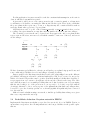
The electricity power network can be depicted as follows; pp1 is the only power plant in this
region, w1–9 are the wires, n1–4 are nodes in which a number of wires are connected, and v1–v4
are the villages.
~~~~~~
||
__
#######
w1
w2
w3
w4
/||\
##pp1##---------(n1)---------(n2)---------(n3)---------[v3]
#######
|
|
|
#######
| w5
| w6
| w7
|
|
|
|
__
__
(n4)
/||\
/||\
/
\
[v1]
[v2]
w8 /
\ w9
/
\
__
__
/||\
/||\
[v4]
[v5]
We have elementary probabilities for each wire as well as the power plant being up and down, and
some conditional probabilities for nodes and villages of having electricity.
Draw a graph for the Bayesian network that describes the relationships between the different
probabilities, and suggest reasonable conditional truth tables. NB: You do not need to use probabilities of 1.0 an 0.0 only as there may be positive (but likely small) probability that electricity do
not propagate from one location to an adjacent even in case the connection wire is up. The other
way round, there may be a very small probability that a node has electricity even of reports saying
that the wire leading to it, or the previous node, are reported to be down (or reported without
electricity); this may be due to wrong reports or the (unusual) incident that some villagers have
been able to get some electricity generator to work and (against all regulations!) have connected
it to the network.
Make a forward calculation using you network, to find the probability that v4 has power, given
that every component in the net is up.
5.2
Probabilistic abduction: Bayesian network in PRISM
Implement the Bayesian network that you produced in exercise 4.1 above in PRISM. Test in on
queries that corresponds to the following situations to find out probabilities for the possible explanations.
13
• v3 is the only one without power.
• v3 is without power; we lack information about v2; anyone else has power.
• v2 and v3 are without power; anyone else has power.
• v4 and v5 has power; anyone else has no power.
• No-one has power.
• Is it possible to query you network for the following, and how: What is the probability that
v2 has power, given that v3 has no power.
5.3
Changing the model to fit reality
It may be case that the answers you get from the model you have produced above, gives unexpected
results. A low prior probability for each wire being down, means that the probability of two wires
being down at the same time is extremely low. This may result in unusual answers being generated
as the most probable ones. Try to identify such cases.
In order to get more reasonable results, we may take into account that the events of the different
wires being down are not independent. If one wire is down, it may be caused by bad weather
conditions, and this may also cause other wires to be down.
Extend your model with a new random variable as follows and use it to condition the wite
status variables; redo the tests of the previous question.
values(weather,[goodWeather,badWeather]).
References
[1] Eugene Charniak. Bayesian networks without tears. AI Magazine, 12(4):50–63, 1991.
[2] Eugene Charniak. Statistical Language Learning. The MIT Press, 1993.
[3] Henning Christiansen and Christina Mackeprang Dahmcke. A machine learning approach to
test data generation: A case study in evaluation of gene finders. In Petra Perner, editor, Proc.
International Conference on Machine Learning and Data Mining MLDM’2007, volume 4571
of Lecture Notes in Computer Science, pages 742–755. Springer, 2007.
[4] Shai Fine, Yoram Singer, and Naftali Tishby. The hierarchical hidden markov model: Analysis
and applications. Machine Learning, 32(1):41–62, 1998.
[5] Finn Verner Jensen. Introduction to Bayesian Networks. Springer-Verlag, 2002.
[6] R.E. Neapolitan. Learning Bayesian Networks. Prentice Hall, 2004.
[7] Taisuke Sato. PRISM, PRogramming In Statistical Modeling; web site, 2007. http://satowww.cs.titech.ac.jp/prism/.
[8] Taisuke Sato and Yoshitaka Kameya. Parameter learning of logic programs for symbolicstatistical modeling. J. Artif. Intell. Res. (JAIR), 15:391–454, 2001.
14
[9] Taisuke Sato and Yoshitaka Kameya. Statistical abduction with tabulation. In Antonis C.
Kakas and Fariba Sadri, editors, Computational Logic: Logic Programming and Beyond, volume 2408 of Lecture Notes in Computer Science, pages 567–587. Springer, 2002.
[10] Neng-Fa Zhou. B-Prolog web site, 1994–2007. http://www.probp.com/.
15