Download ADAS301: State selective charge exchange data

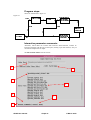
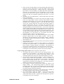
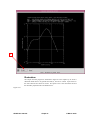
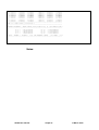
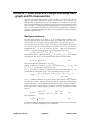
ADAS301: State selective charge exchange data
- graph and fit cross-section
The code interrogates state selective charge exchange cross-section files of type
ADF01. Data may be extracted for capture to a selected n-, nl-or nlm-shell of a
hydrogen-like or lithium-like receiving ion depending on the ADF01 file. The data
may be interpolated using cubic splines to provide cross-sections at arbitrarily chosen
impact energies. A minimax polynomial approximation is also made to the source
data. The source and interpolated cross-section data are displayed and a tabulation
prepared. The tabular and graphical output may be printed and include the minimax
polynomial approximation.
Background theory:
The code allows display of the total, n-, nl, or nlm-shell charge exchange crosssections depending on the data resolution of the input ADF01 file. Most files are at
nl-shell resolution. The full prescription of the data sets are given in the appxa-01.
For a specified relative collision energy Ei belonging to the tabulation, let the total
cross section be σ tot ( E i ) and the n-shell cross-sections be σ n ( Ei ) . The latter are
tabulated for nmin ≤ n ≤ nmax for some nmin and nmax . Data can be displayed for
n ≥ nmax . To achieve this the program uses an extrapolation of the form
σ n ( Ei ) = (nmax / n ) β( Ei ) σ nmax ( Ei )
4.1.1
The parameter β ( Ei ) is deduced from σ nmax −1 ( Ei ) and σ nmax ( Ei ) . It is tabulated
in the data set. The σ n ( Ei ) are normalised to the total cross-section so that
σ tot ( Ei ) =
∝
∑σ
n
( Ei )
4.1.2
n = nmin
using the extrapolation equation 4.1.1 for n ≥ nmax .
Explicit l-subshell cross-sections σ nl ( Ei ) are tabulated for nmin ≤ n ≤ nmax and
0 ≤ l ≤ n − 1. In extrapolation there are two cases.
Case 1: No l subshell subdivision parameters are given in the ADF01 dataset.. It is
assumed that the l distribution for n > nmax is the same as for nmax so that
σ n l ( Ei )(σ n ( Ei ) / σ nmax ( E i )) for l ≤ n max − 1
σ nl ( Ei ) =  max
0
for l ≥ n max

4.1.3
Case 2: l subshell parameters are given in the the ADF01 dataset. The parameters
are obtained as a fit to l- subshell cross-section data for a particular n-shell using the
program ADAS107. The parameterisation identifies an l-type , parameter ltyp ( Ei )
and an approximate l (non integral) at which the cross-section behaviour changes
from rising at low l to falling at high l, parameter xlcr ( Ei ) . The behaviour is then
given by
(2l + 1) pl 2
σ nl ( Ei ) ~ 
pl 3
 exp( − (l − xlcr ) )
The normalisation
for l < xlcr
for l < xlcr
4.1.4
n −1
σ n ( Ei ) = ∑ σ nl ( Ei )
4.1.5
l =0
is maintained while the sharpness of the switching between the two forms varies with
the l-type. A detailed description is given in ADAS107.
ADAS User manual
Chap4-01
17 March 2003
Program steps:
These are summarised in figure 4.1.
Figure 4.1
EHJLQ
!
VHOHFW 4&; ILOH
HQWHU ILW FKRLFHV
UHDG DQG YHULI\
!
!
4&; ILOH
VHOHFW VKHOO DQG
RXWSXW HQHUJLHV
UHSHDW
UHSHDW
FRPSXWH FXELF
!
VSOLQH DQG
!
PLQLPD[ ILW
2XWSXW WDEOHV
DQG JUDSKV
HQG
GLVSOD\ FKDUJH
H[FKDQJH FURVV
VHFWLRQ JUDSK
Interactive parameter comments:
ADAS301, which make use of data from archived ADAS datasets, initiates an
interactive dialogue with the user in three parts, namely, input file selection, entry of
user data and disposition of output.
The file selection window is shown below.
1
2
4
3
5
7
6
ADAS User manual
Chap4-01
17 March 2003
1.
2.
3.
4.
5.
6.
7.
Data root shows the full pathway to the appropriate data subdirectories.
Click the Central Data button to insert the default central ADAS
pathway to the correct data type – ADF01 in this case. Note that each
type of data is stored according to its ADAS data format (adf number).
Click the User Data button to insert the pathway to your own data.
Note that your data must be held in a similar file structure to central
ADAS, but with your identifier replacing the first adas, to use this
facility.
The Data root can be edited directly. Click the Edit Path Name button
first to permit editing.
Available sub-directories are shown in the large file display window.
There are a large number of these, stored by donor which is usually
neutral but not necessarily so (eg. qcx#h0). The individual members are
identified by the subdirectory name, a code and then fully ionised
receiver (eg. qcx#h0_old#c6.dat). The data sets generally contain nlresolved cross-section data but n-resolved and nlm-resolved are
handled. Resolution levels must not be mixed in datasets. The codes
distinguish different sources.The first letter o or the code old has been
used to indicate that the data has been produced from JET compilations
which originally had parametrised l-distribution of cross-sections. The
nl-resolved data with such code has been reconstituted from them. Data
of code old is the preferred JET data. Other sources codes include ory
(old Ryufuku), ool (old Olson), ofr (old Fritsch) and omo (old
molecular orbital). There are new data such as kvi.
Click on a name to select it. The selected name appears in the smaller
selection window above the file display window. Then its subdirectories in turn are displayed in the file display window. Ultimately
the individual datafiles are presented for selection. Datafiles all have
the termination .dat.
Once a data file is selected, the set of buttons at the bottom of the main
window become active.
Clicking on the Browse Comments button displays any information
stored with the selected datafile. It is important to use this facility to
find out what is broadly available in the dataset. The possibility of
browsing the comments appears in the subsequent main window also.
Clicking the Done button moves you forward to the next window.
Clicking the Cancel button takes you back to the previous window
The processing options window has the appearance shown below
1. An arbitrary title may be given for the case being processed. For
information the full pathway to the dataset being analysed is also
shown. The button Browse Comments again allows display of the
information field section at the foot of the selected dataset, if it exists.
2. The output data extracted from the datafile, a ‘charge exchange crosssection’, may be fitted with a polynomial. This is as a function of
relative collision energy per atomic mass unit (eV/amu). Clicking the
Fit Polynomial button activates this. The accuracy of the fitting
required may be specified in the editable box. The value in the box is
editable only if the Fit Polynomial button is active
3. Your settings of collision velocity/energy (output) are shown in the
display window. The velocity/energy values at which the charge
exchange coefficients are stored in the datafile (input) are also shown
for information. The program recovers the output velocities/energies
you used when last executing the program.
4. Pressing the Default Velocity/Energy values button inserts a default set
of velocities/energies equal to the input velocities/energies
5. The Velocity/Energy values are editable. Click on the Edit Table
button if you wish to change the values. A ‘drop-down’ window, the
ADAS Table Editor window: It follows the same pattern of operation
as described in the 18nov-94 bulletin.
ADAS User manual
Chap4-01
17 March 2003
6.
7.
8.
The specific cross-section data to be extracted is specified by the
window to the right. The level or resolution of the data source is
shown.
Activate the Select quantun numbers for processing button to allow new
settings of these quantum numbers. The values in the three smaller
windowsbecome editable depending also on the resolution of the
dataset. Note that the Range of the data in the dataset is displayed.
There are special codes to be used to obtain summed cross-sections
over sub-quantum numbers. These are indicated in brackets under the
Total column and should be entered into the editable window if
required.
1
7
8
2
3
4
5
6
9
9.
Clicking the Done button causes the next output options window to be
displayed. Remember that Cancel takes you back to the previous
window.
The output options window is shown below
1.
2.
3.
ADAS User manual
As in the previous window, the full pathway to the file being analysed
is shown for information. Also the Browse comments button is
available.
Graphical display is activated by the Graphical Output button. This
will cause a graph to be displayed following completion of this window.
When graphical display is active, an arbitrary title may be entered
which appears on the top line of the displayed graph.
By default, graph scaling is adjusted to match the required outputs.
Press the Explicit Scaling button to allow explicit minima and maxima
for the graph axes to be inserted. Activating this button makes the
minimum and maximum boxes editable.
Chap4-01
17 March 2003
4.
5.
6.
Hard copy is activated by the Enable Hard Copy button. The File name
box then becomes editable. If the output graphic file already exits and
the Replace button has not been activated, a ‘pop-up’ window issues a
warning.
A choice of output graph plotting devices is given in the Device list
window. Clicking on the required device selects it. It appears in the
selection window above the Device list window.
The Text Output button activates writing to a text output file. The file
name may be entered in the editable File name box when Text Output is
on. The default file name ‘paper.txt’ may be set by pressing the button
Default file name. A ‘pop-up’ window issues a warning if the file
already exists and the Replace button has not been activated.
1
2
3
5
4
6
The Graphical output window is shown below
1. Printing of the currently displayed graph is activated by the Print button.
ADAS User manual
Chap4-01
17 March 2003
1
Illustration:
The output from the program is illustrated in figure 4.1a for capture by H+ from a
deuterium beam atom in its ground state D0(1s), into the n=4 shell. Input values in
the source data set are shown as crosses. The spline curve is the continuous line and
the minimax polynomial fit is the dashed curve.
Figure 4.1a
ADAS User manual
Chap4-01
17 March 2003
The tabular output is shown in table 4.1a. Output data which requires extrapolation
beyond the range of the original data in the source ADF01 file are indicated by *
when necessary. The rate coefficient is obtained from the cross-section by simply
multiplying by the collision speed.
Table 4.1a
ADAS RELEASE: ADAS98 V2.5.6 PROGRAM: ADAS301 V1.10 DATE: 24/11/02 TIME: 10:19
******* TABULAR OUTPUT FROM CHARGE EXCHANGE CROSS-SECTION INTERROGATION PROGRAM: ADAS301 - DATE: 24/11/02 *********
-------------------
ADAS User manual example
-------------------
CHARGE EXCHANGE CROSS-SECTIONS AS A FUNCTION OF ENERGY
------------------------------------------------------DATA GENERATED USING PROGRAM: ADAS301
------------------------------------/packages/adas/adas/adf01/qcx#h0/qcx#h0_old#n7.dat
FILE IS L RESOLVED
- SUB-B
PRINCIPAL QUANTUM N-SHELL = 7
ORBITAL
QUANTUM L-SHELL = 3
-- ENERGY -- -------- VELOCITY -------- ----- CROSS-SECTION ----- RATE COEFFT
eV/amu
at.units
cm/sec
cm**2
pi*(a0**2)
cm**3/sec
------------------------------------------------------------------------------1.000D+03
2.008D-01
4.393D+07
7.830D-19
8.900D-03
3.440D-11
1.500D+03
2.459D-01
5.380D+07
2.130D-18
2.421D-02
1.146D-10
2.000D+03
2.840D-01
6.212D+07
3.810D-18
4.331D-02
2.367D-10
3.000D+03
3.478D-01
7.609D+07
5.510D-18
6.263D-02
4.192D-10
5.000D+03
4.490D-01
9.823D+07
5.680D-18
6.456D-02
5.579D-10
7.000D+03
5.313D-01
1.162D+08
6.200D-18
7.048D-02
7.206D-10
1.000D+04
6.350D-01
1.389D+08
7.910D-18
8.991D-02
1.099D-09
1.500D+04
7.777D-01
1.701D+08
1.360D-17
1.546D-01
2.314D-09
2.000D+04
8.980D-01
1.965D+08
2.250D-17
2.558D-01
4.420D-09
3.000D+04
1.100D+00
2.406D+08
3.790D-17
4.308D-01
9.119D-09
ADAS User manual
Chap4-01
17 March 2003
5.000D+04
1.420D+00
3.106D+08
3.540D-17
4.024D-01
1.100D-08
6.000D+04
1.555D+00
3.403D+08
2.990D-17
3.399D-01
1.017D-08
7.000D+04
1.680D+00
3.675D+08
2.230D-17
2.535D-01
8.196D-09
4.000D+04
1.270D+00
2.778D+08
4.050D-17
4.604D-01
1.125D-08
8.000D+04
1.796D+00
3.929D+08
1.700D-17
1.932D-01
6.679D-09
1.000D+05
2.008D+00
4.393D+08
9.460D-18
1.075D-01
4.156D-09
1.500D+05
2.459D+00
5.380D+08
3.860D-18
4.388D-02
2.077D-09
2.000D+05
2.840D+00
6.212D+08
1.900D-18
2.160D-02
1.180D-09
3.000D+05
3.478D+00
7.609D+08
7.430D-19
8.446D-03
5.653D-10
------------------------------------------------------------------------------KEY: a0 => Bohr radius = 5.29177D-11 m
------------------------------------------------------------------------------MINIMAX POLYNOMIAL - TAYLOR COEFTS: LOG10(X-SEC<cm**2>) vs. LOG10(ENGY<eV/amu>)
------------------------------------------------------------------------------A( 1) =
2.267736763D+04
A( 2) = -3.960306568D+04
A( 3) =
2.930884365D+04
A( 4) = -1.192631460D+04
A( 5) =
2.882343432D+03
A( 6) = -4.138118687D+02
A( 7) =
3.268644382D+01
A( 8) = -1.096179853D+00
LOGFIT - DEGREE= 7 ACCURACY= 4.34% END GRADIENT: LOWER=
1.82 UPPER= -3.52
-------------------------------------------------------------------------------
Notes:
ADAS User manual
Chap4-01
17 March 2003