Download TCD-CS-2006-68 - School of Computer Science and Statistics

Hopping: A Bidirectional Stigmergy Power Efficient
On-Demand Driven Ad Hoc Routing Protocol for
Wireless Sensor Networks
Ricardo Simon Carbajo
A dissertation submitted to the University of Dublin,
in partial fulfillment of the requirements for the degree of
Master of Science in Computer Science
September 2006
Declaration
I declare that the work described in this dissertation is,
except where otherwise stated, entirely my own work and
has not been submitted as an exercise for a degree at this
or any other university.
Signed: ___________________
Ricardo Simon Carbajo
11th September 2006
i
Permission to lend and/or copy
I agree that Trinity College Library may lend or copy this
dissertation upon request.
Signed: ___________________
Ricardo Simon Carbajo
11th September 2006
ii
Acknowledgements
First of all, I would like to thank my supervisor Meriel Huggard, she has been there
when I needed, she has opened my mind and it has been a pleasure working with
her.
Besides, I would like to thank Dr. Ciaran Mc Goldrick and Mathieu Robin for
providing me with their advice.
In the family environment I want to thank, not only my family (mother, father,
brother, sister, aunts, grandmothers and uncles) who has been supporting me during
all this Msc process and encouraging me to keep going, but also the people I know
in Ireland, specially my Irish family who has been very close to me.
Finally, I can not forget the whole of NDS class with whom I have lived an
amazing experience, academically and personally, and where I have made good
friends.
iii
Abstract
According to Bell’s Law, it emerges a new technology every ten years. In February
2003, the MIT identified the top ten emerging technologies that will change the
world; Wireless Sensor Networks (WSN) was the first one.
Wireless Sensor Networks appear like a favorite candidate to create a new era of
information in which everything will be controlled by sensors monitoring the
environment and acting appropriately; all of that to facilitate our modern living.
It is a new technology based in sensors communicating wirelessly with each
other and sensing data from the environment to processing units. If this technology
is combined with Artificial Intelligence it is believed that worldwide auto-organized
networks will control everything.
Because the communication is an important issue of WSN, the aim of this
project has been focused on the improvement of ad hoc protocols which suite the
needs and constraints of this technology. Research has been done over the area,
concerning about differences with respect to traditional wired networks. Besides, it
has been examined previously created ad hoc protocols for WSN.
After all the research process, keeping in mind the features of WSN, it has been
developed a new protocol which addresses constraints like power and storage
limitations, guaranteeing bidirectional communication between nodes. It is thought
this protocol will improve the communication in WSN, avoiding hierarchy schemas,
with nodes communicating with each other in an ad hoc basis paradigm to create
self-organized colonies; all of this in an efficient way, with a low energy
consumption and minimum data storage.
iv
Table of Contents
DECLARATION .........................................................................................................I
PERMISSION TO LEND AND/OR COPY.............................................................. II
ACKNOWLEDGEMENTS...................................................................................... III
ABSTRACT..............................................................................................................IV
TABLE OF CONTENTS........................................................................................... V
LIST OF FIGURES ............................................................................................... VIII
LIST OF TABLES..................................................................................................... X
CHAPTER 1 – INTRODUCTION .............................................................................1
CHAPTER 2 – INTRODUCTION TO WIRELESS SENSOR NETWORKS (WSN)
....................................................................................................................................4
2.1- SENSORNET VISION ...................................................................................................................4
2.2- WHAT IS A WIRELESS SENSOR NETWORK? ................................................................................5
2.3- WHAT IS A MOTE?......................................................................................................................6
2.4- CHARACTERISTICS OF A WIRELESS SENSOR NETWORK .............................................................9
2.4.1- Strengths ...........................................................................................................................9
2.4.2- Constraints and Weaknesses ...........................................................................................11
2.5- APPLICATIONS .........................................................................................................................12
2.6 – NESC AND TINYOS ................................................................................................................15
2.6.1- NesC................................................................................................................................15
2.6.2- TinyOS ............................................................................................................................18
CHAPTER 3 – AD HOC ROUTING PROTOCOLS...............................................22
3.1- INTRODUCTION ........................................................................................................................22
3.2- GRAPH BASED ROUTING ...........................................................................................................22
3.2.1- Bellman-Ford..................................................................................................................22
3.2.2- Dijkstra ...........................................................................................................................23
3.2.3- Min-Hop Algorithm.........................................................................................................23
3.3- AD HOC ROUTING PROTOCOLS ................................................................................................24
3.3.1- Routing classification 1...................................................................................................24
3.3.2- Routing classification 2...................................................................................................25
v
3.3.3- OLSR (Optimization Link State Routing) Algorithm.......................................................27
3.3.4- Direct Diffusion Algorithm .............................................................................................28
3.3.5- Rumor-based Algorithm..................................................................................................29
3.4- LINK STATE ESTIMATION ........................................................................................................32
3.4.1- EWMA (Exponentially Weighted Moving Average)........................................................32
3.4.2- Flip-Flop EWMA ............................................................................................................33
3.4.3- WMEWMA (Windows Mean EWMA)..............................................................................33
CHAPTER 4: ROUTING IN TINYOS ....................................................................35
4.1- INTRODUCTION ........................................................................................................................35
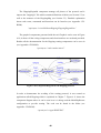
4.2- ARCHITECTURE OF THE AD HOC ROUTING COMPONENT ..........................................................36
4.3- EWMA MULTI HOP ROUTER ALGORITHM (THE 1ST ONE) ........................................................37
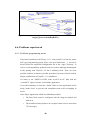
4.4- WMEWMA MULTI HOP ROUTER ALGORITHM (THE 2ND ONE) ................................................38
4.4.1- Interface Description ......................................................................................................39
4.4.2- Component Description ..................................................................................................39
4.5- STRUCTURE OF THE MULTIHOP MESSAGE .................................................................................41
4.6- SENDING A PACKET ..................................................................................................................42
4.7- RECEIVING A PACKET ..............................................................................................................43
4.8- OTHER ROUTING COMPONENT PROJECTS ................................................................................43
4.9- NEW RECENTLY RELEASED ROUTING ALGORITHMS (TINYOS V2.0).......................................43
4.9.1- Collection........................................................................................................................44
4.9.2- Dissemination .................................................................................................................45
CHAPTER 5: HOPPING - A BIDIRECTIONAL STIGMERGY POWER
EFFICIENT ON-DEMAND DRIVEN AD HOC ROUTING PROTOCOL ...........46
5.1- CONSTRAINTS TO ADDRESS IN ROUTING ON SENSORNET ........................................................46
5.2- THE PROTOCOL BASIS ..............................................................................................................47
5.3- HOPPING AM MESSAGE STRUCTURE ........................................................................................49
5.4- THE PROCEDURE, HOW THE PROTOCOL WORKS ........................................................................50
-
Phase1 (Discover Route) .................................................................................................50
-
Phase 2 (Follow Route) ...................................................................................................52
-
Phase 3 (Garbage Collector)...........................................................................................53
5.5- FEATURES AND DRAWBACKS OF THE PROTOCOL ......................................................................54
CHAPTER 6 – DEVELOPING THE PROTOCOL ON WIRELESS SENSOR
NETWORKS ............................................................................................................55
6.1- INTRODUCTION ........................................................................................................................55
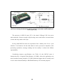
6.2- HARDWARE .............................................................................................................................55
6.2.1- Motes...............................................................................................................................55
6.2.2- Programming Board – Gateway .....................................................................................58
vi
6.2.3- Sensor Boards .................................................................................................................59
6.3- SOFTWARE ...............................................................................................................................60
6.4- START UP A WSN WITH TINYOS AND CROSSBOW MOTES .......................................................62
6.5- DESIGN AND IMPLEMENTATION OF HOPPING ...........................................................................66
6.6- PROBLEMS EXPERIENCED .........................................................................................................69
6.6.1- Problems programming motes ........................................................................................69
6.6.2- Problem using the multihop components ........................................................................70
CHAPTER 7 – EVALUATION ...............................................................................72
CHAPTER 8 - CONCLUSIONS AND FUTURE RESEARCH..............................75
REFERENCES .........................................................................................................77
APPENDIX: CD-ROM.............................................................................................80
vii
List of Figures
Figure 2.1: Wireless Sensor Network [5] ...................................................................6
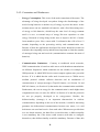
Figure 2.2: Wireless Sensor Network in the Great Duck Island, monitoring the
storm petrel (seabird). From 1 to 5 it indicates the process of transmitting data
from the motes to the gateway and finally to the satellite [10].........................13
Figure 2.3: TinyOS component layer architecture [16]............................................19
Figure 3.1: The agent modifies the exist path to a more optimal one [23]...............30
Figure 3.2: When agent prorogation the path to Event 2 comes across a path to
Event 1, it begins to propagate the aggregate path to both [23.........................31
Figure 3.3: Query is originated from the query source and searches for a path to the
event. As soon as it finds a node on the path, it’s routed directly to the event
[23]....................................................................................................................32
Figure 4.1: Component Architecture [26].................................................................36
Figure 4.2: MultiHopRouter configuration [27] .......................................................38
Figure 4.3: AM_MULTIHOP message structure .....................................................41
Figure 4.4: TOS_Msg message structure..................................................................42
Figure 5.1: AM_HOPPINGMSG message structure................................................49
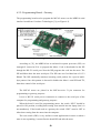
Figure 6.1: Left: Photo of a MICA2 (MPR4x0) without an antenna. Right: Top and
plan views showing the dimensions and hole locations of the MICA2 PCB
without the battery pack. [34] ...........................................................................56
Figure 6.2: Programming Board MIB510CA [34] ...................................................58
Figure 6.3: MICA Sensor Board MTS300CA [36] ..................................................59
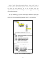
Figure 6.4: TinyOS and Subdirectory Map [13].......................................................61
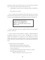
Figure 6.5: Makelocal file in folder “/apps” in TinyOS ...........................................63
Figure 6.6: Compilation & Load application into a mica2 mote. .............................65
Figure 6.7: SerialForwarder Tool .............................................................................65
Figure 6.8: Surge application using multihop routing in TinyOS ............................66
Figure 6.9: MultiHopRouter configuration for the Hopping protocol......................67
Figure 6.10: Component Diagram for the Hopping protocol. ..................................68
viii
Figure 6.11: Component Diagram for the Hopping application which uses the
Hopping protocol (MultiHopRouter)................................................................69
Figure 6.12: Modifications (in bold) in the MutiHopEngineM component to allow
functionality in the event Receive.receive. .......................................................71
ix
List of Tables
Table 2.1: Different type of motes used in TinyOS research [7]................................8
Table 2.2: Description of the main TinyOS/nesC components [13].........................18
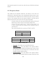
Table 5.1: Reachable Motes......................................................................................47
Table 5.2: Routing Table ..........................................................................................47
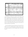
Table 6.1: Mote Specifications Summary [34].........................................................57
x
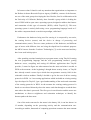
Chapter 1 – Introduction
According to Bell’s Law, it emerges a new technology every ten years. In
February 2003, the MIT identified the top ten emerging technologies that will
change the world; Wireless Sensor Networks (WSN) was the first one.
Experts presume it is going to be a new era of information, leaded by sensors
acting and retrieving data in all different types of environments, from a house to a
volcano three kilometers meter high.
These sensors, which can have mobility, will have the capacity to communicate
wirelessly each other forming networks which will control an area, a country or
even the world.
Taking profit of the Internet infrastructure combined with Wireless Sensor
Networks everyplace will be reachable and monitored.
Besides, if Artificial Intelligence is combined with this infrastructure, it could be
created self-managed networks which monitor, analyze and take decisions for the
benefit of the human being.
It could sound like science fiction but it is believed it can be a reality and in fact,
in the actual world are examples that indicate so. Intelligent Buildings completely
equipped with sensors which tell when a fire is produced is just an example of the
daily life with sensors but if you add the power of wireless to reach any place and
the capacity of a sensor device to act as a processing unit which have enough
autonomy to join networks, then new potential possibilities are open.
After assisting lectures about the topic, reading articles in Internet and the
dissertation from Karsten Fritsche titled: “TinyTorrent: Combining BitTorrent and
SensorNets” [1], I became really interested in Wireless Sensor Networks. I started
to do research in how it works, possible applications, which groups are working on
it, what systems are leading the panorama and mainly what needs or possibilities are
offered.
1
In between what I found it took my attention that organizations as important as
the Defense Advance Research Projects Agency (DARPA), creators of the Internet,
are one of the main groups developing the idea. Besides, Intel in collaboration with
the University of California, Berkeley have founded a group which is leading the
area of WSN with its open source operating system, designed to address the features
and constraints of this type of networks (WSN), called TinyOS [2]. This new
operating system is entirely built using a new programming language based on C
but with a component based event-driven paradigm, called nesC.
Furthermore the hardware being used for sensing it is composed by two units,
the sensing devices (sensor) and the device in charge of processing and
communications (mote). There are some producers of this hardware, and different
type of motes with different sizes are being developed but for academic purposes
the MICA2 motes from the Crossbow Technologies [3] are the most used and they
have been used in this project.
After spending sessions learning how to program motes, using TinyOS, learning
the new programming language and the new programming structure, getting
hardware errors, compiling and testing all different applications that TinyOS
provides, I started to figure out what attracted me the most and what is needed in
WSN at the moment. At the beginning I thought about security issues, as TinyOS
have already created a secure layer which does not guarantee security 100% in the
vulnerable wireless medium. Finally I decided to go for the area of ad hoc routing
protocols in WSN. As I was testing applications which included an existing routing
layer developed in TinyOS, I got a good understanding of the needs and constraints
of the routing protocols in WSN. At the moment the existing routing protocol is
based on a tree-based hierarchy where the motes send data through to reach the base
mote where the data is processed. The flow goes in one direction and the motes use
mechanisms to discover neighbours and estimation techniques to identify the
shortest path to the base mote.
One of the main concerns for the motes is the battery life; it can last about 6 to
12 months, depending on the processing activity and the communication rate.
According to studies, thousands of computing operations consume the same amount
2
of energy as one message sent. Because of that the idea was to minimize the number
of messages needed in all the phases of the routing protocol; in the existing
protocol, every 20 seconds a broadcast discovery message is sent to identify the
neighbours.
After all of that and studying different ad hoc routing protocols like rumor based
and stigmergy techniques, the protocol (hopping) was designed. The protocol try to
address constraints of battery life by reducing the number of messages being sent
and all of that considering the limited resources of the motes. Besides, it was
thought applying stigmergy could be a good idea; the paths between motes are
created by modifications in the environment, it is said in every mote which is part of
a well established path, it will be an entry for this path which indicates who the
sender is and where it should be sent the message.
In the rest of the document it will be explained in detail what technology is
currently being used in Wireless Sensor Networks, hardware and software. It will be
described the main routing algorithms which inspired the creation of the protocol.
An analysis and good description of the routing layer in TinyOS will be made and
the protocol in details will be described. Finally it will be commented what
technology has been used and the process of implementation and debugging of the
algorithm, making an evaluation of it; conclusions and future research will be stated
to finish.
3
Chapter 2 – Introduction to Wireless Sensor
Networks (WSN)
2.1- SensorNet Vision
We are leaving in the world of information where data is available to everybody but
obtaining the data which is needed at a certain time is a mayor deal. In order to get
the best advantage, the data should come from different sources of interest and
relationships should be established to transform it in what is called information.
There are several ways of getting data from the environment but the most well
known technique is called “monitoring”. The process of monitoring according to [4]
involves observing a situation for any changes which may occur over time, using a
monitor or a measuring device. This measuring device is what we call sensor; any
instrument that can retrieve diverse type of data like temperature, humidity,
pressure, flow, length, speed, sound, light… and transform into an electronic data
which can be processed or retransmitted.
These sensors are everywhere at the moment, from houses to companies or even
roads but there are some limitations, they usually depends on powered processing
systems and have to be wired to them. These constraints limit the monitoring
process to certain environment with specific conditions.
According to Moore’s Law (posited by Intel founder Gordon Moore in 1965)
[5], the number of transistors on a chip roughly doubles every two years, resulting
in more features, increased performance and decreased cost per transistor. Not only
the devices have more powerful processing and are cheaper but also they provide
new features like wireless communication combined with a very small size.
Because of that, it is being created a new class of monitoring systems which can
get a wide range of diversity data that can be converted into a new generation of
information, rich in semantic content.
Quoting [5], “These inexpensive, low-power communication devices can be
deployed throughout a physical space, providing dense sensing close to physical
phenomena, processing and communicating this information, and coordinating
4
actions with other nodes. Combining these capabilities with the system software
technology that forms the Internet makes it possible to instrument the world with
increasing fidelity”.
David Culler et al [5] state that because of the fact that the world of computing
is becoming throw the high processing and miniaturization, there is a new
revolution emerging in the form of small cheap devices capable of processing and
communicate wirelessly, that can be spread in any environment and interact, not
only each other forming networks, but also with the Internet, in order to monitor the
world and act accordingly.
All this new technology is what is emerging and is what is known as Wireless
SensorNet; collection of interconnected devices with sensing, processing and
communication capabilities which can retrieve many types of data, auto-organising
and behave in a ubiquitous way.
The wireless sensor network regime is characterized by some constrains like
limited hardware capabilities, limited energy resources and concurrent data flows
which lead to a mandatory change or adaptation from the actual technology vision.
Because of the limitations in hardware and power, key concepts like programming
paradigms, OS, networking, data management, security, etc…, should be addressed
with special constrains too.
In the nearest future, this technology could generate nets all over the planet that
will watch from what the people buy at the supermarkets to malicious people. If we
put together this technology with the new advances in Artificial Intelligence it could
be created networks of sensors with complex intelligence.
2.2- What is a Wireless Sensor Network?
A Wireless Sensor Network is a set of tiny, battery-powered sensing devices which
are usually called “motes” or “smart dust”.
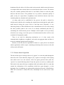
Typically these motes are spread in groups all over a certain physical
environment. Once they are positioned, they start to connect each other wirelessly
and organize them into a network (see Figure 2.1). Each mote has a radio area and
all the nodes on the area are considered neighbours. Using the neighbours and ad
hoc routing protocols (the motes can have mobility), the sensor starts to retrieve
5
data from the environment (light, temperature, vibration…) and provides it to the
mote unit which will manage the processing, wrapping of the messages and
communication with the neighbours in order to send the data through the different
motes over the network in order to reach the base node. The base node is a special
mote, because it is connected to a processing station, usually traditional computers,
where the data from the motes in the network is analyzed, making possible the
creation of a picture of the environment in real time as well as the publication of the
information in the Internet.
Retrieving data from the environment is the most frequent use for WSN
although the interaction with the motes from the computer and even from the
Internet is being developed; new protocols are needed to communicate in both
directions.
Figure 2.1: Wireless Sensor Network [5]
2.3- What is a mote?
Typically a mote is a little device whose main tasks are: to sense (with the sensor
attached to the mote), to compute and to communicate. According to that, motes
have three main components:
-
Microprocessor: process the data.
-
Microelectromechanical systems (MEMS): provide arrays of sensory
measures.
-
Low-power Radios (transceivers): wireless communication.
6
There are many types, depending on the fabricant, with different forms and
sizes. In Table 2.1, it can be seen different types of motes with its specifications
used in researching with the TinyOS operating system (see Section 2.6).
Besides, depending on the type of mote, standard consumer AA or coin-style
batteries keep motes “alive” for six months to a year, although new research is being
doing on that using new energy sources like the solar one.
Common design constraints include:
-
power conservation
-
compact form
-
limited memory
-
limited storage capacity
Moreover, and according to [6], motes must be reasonably economical to be
suitable for practical applications. Fortunately, microprocessors, sensors and RF
transceivers can be inexpensively produced in large quantities using conventional
semiconductor manufacturing techniques. Several species of motes based on
prototypes developed by Intel and the University of California at Berkeley have
recently become commercially available at $50 to $100 (U.S.) each. Researchers at
Intel expect that, with re-engineering, Moore’s Law and volume production, motes
could drop in price to less than $5 each over the next several years.
7
The weC Node
The weC node was developed in the Fall of 1999 by
researchers at UC Berkeley. It containes 8K of program
memory and just 512 bytes of memory. On-board
temperature and light data could be wirelessly
communicated over it 9600 baud on-off keyed radio. An
internal antenna provided a range of up to 15 feet.
The Rene Node
Developed in the summer of 2000, Rene node expanded on
the capabilities of the weC node by increasing available
program and data storage. Additionally, it provided a 51pin expansion interface that allow for connections to both
analog and digital sensors. As a development platform,
hundreds of sensor boards have been designed to interface
to the Rene node. It is equipped with 8K of program
memory, 32K of EEProm and is capable of being
reprogrammed over the radio link. It communicates at
19,200 via an on-off keyed 916 Mhz radio. An external
antenna allows for a communication rage of up to 100 feet.
The DOT Node
Developed in the summer of 2001, Dot shrunk the
capabilities of the Rene node into a compact 1” node. A
complete node including sensor, computation,
communication, and a battery fit in a package the size of
four stacked quarters. It was unveiled at the 2001 Intel
Developers Forum in as the cornerstone of an 800 node
demonstration network. The Dot platform had 16 KB of
program memory and 1 K of data memory. It had the same
communication capabilities of the Rene platform.
The Mica node was developed as the foundation of the
NEST (Network Embedded Systems Technology) project
under DARPA (Defense Advanced Research Projects
Agency). Designed to facilitate the exploration of wireless
sensor networking, it has been used by over 200 different
research organizations. Mica contains the same expansion
bus as the Rene node allowing it to utilize all existing
sensor boards. The Mica node increases the radio
communication rate to 40 Kbps though using specialized
hardware accelerators and amplitude-shift-keying. Mica
includes 128 Kbps of program memory and 4 K of data
memory. It is capable of being radio-reprogrammed and
has a line-of-sight rage of over 100 feet. Mica has been
used in applications ranging from military vehicle tracking
to remote environmental monitoring.
Spec was designed in the fall of 2002 by Jason Hill to be a
highly integrated, single-chip wireless node. The CPU,
memory, and RF transceiver are all integrated into a single
2.5x2.5mm piece of silicon. Fabricated by National
Semiconductor, it was successfully demonstrated in March
of 2003. Spec contains specialized hardware accelerators
designed to improve the efficiency of multi-hop mesh
networking protocols. Additionally, in includes an ultralow power transmitter that drastically reduces overall
power consumption. Spec represents the future of
embedded wireless networking.
The Mica Node
The Spec Node
Table 2.1: Different type of motes used in TinyOS research [7]
8
2.4- Characteristics of a Wireless Sensor Network
According to [1] WSN research is gaining popularity, due to the exciting
possibilities it opens up to new application domains. Because of that, in this section
will be discussed the strengths of WSN, which give rise to these new possibilities,
and the weaknesses and constraints.
2.4.1- Strengths
-
Harsh environmental conditions: The fact that WSN work wirelessly
makes possible the communication under any environmental circumstance.
Besides if we add that the motes (sensors) are characterized by its reduced
size, the possibilities of reaching small inaccessible places hugely increase.
Furthermore with the advances in technology, motes will be as small as one
of these little letters you are reading now, with enough computing process to
sense, analyze and send data, and all of that powered by batteries combined
with solar energy that will last months or years. Then everything,
everywhere will be monitored.
-
Low Cost and High Production Volumes: In modern industry, the large
volume of production for electronic devices, minimize the cost per unit
extremely. Motes are composed of microcontrollers, sensors and radio
devices which can be developed easily and quickly but in order to reduce its
cost, the volume of production must be huge. Although now the price of
motes is not expensive (depends on model), the cost of spreading hundreds
of motes all over an environment is high; if the technology is consolidated,
the amount of production will increase severely, reducing the size of motes
and the price will go down to some cents per unit being able to spread
thousands of motes with a lower cost. Spreading more motes by surface will
increase the reliability in the system and the measured data would be more
accurate.
9
-
Ad-hoc Deployment: Because of the nature of this technology, motes could
be spread in environments without an already created topology and with
mobility. Consequently WSN need the deploying of ad hoc protocols which
provide communication among the motes to create auto-organized networks,
discovering neighbours and gateways. This is one of the main interesting
points and it is currently being done a lot of research; already existing ad hoc
protocols have to be adapted to address the constraints of this technology. In
this dissertation is developed an ad hoc protocol which addresses some of
this constraints.
-
Fault Tolerance: The fact that motes are hardware which works with events
and concurrency in an autonomous way with radio communication makes
the system lean to failures. To prevent that it has been developed software
mechanisms to avoid or recover from failures (not pure recovery
mechanisms in nodes but it is based on resetting); besides, if the
concentration of motes in the same surface is higher, that will make the
system fault tolerant; more motes could monitor and communicate data of
similar conditions so the failure of a node will not produce a network system
failure.
-
Data Quality: Redundancy makes the system fault tolerance but also makes
the data more reliable and consequently of a better quality.
-
Heterogeneity of nodes: Motes can be different in a network and measure
different values. That improves the feature of scalability in the system and
allows diversity. On the other hand the maintenance or update of motes will
be more difficult.
-
Unattended operation: Wireless Sensor Networks are characterized as selforganized networks which can be deployed in any environment and work
without control of human beings, monitoring and acting over the
environment autonomously and recovering from failures.
10
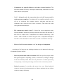
2.4.2- Constraints and Weaknesses
-
Energy Consumption: This is one of the main constraints of the motes. The
advantage of being developed everywhere brings the disadvantage of the
need of using batteries or another way of energy to power the motes. At the
moment motes can use standard AA batteries, with a fixed decreasing curve
of energy or litio batteries, which keep the same level of energy constant
until it is over, or external ways of energy like new capacitors or solar
energy. Research is being doing in this area to improve the life of motes
from months to years. Now, a mote with 2 AA batteries has a life of 6 to 12
months, depending on the processing activity and communication rate.
Because of that, the applications developed for motes should be oriented to
minimize the computing activity and the most important, to limit the number
of messages being sent and received (communications consume the most of
batteries).
-
Communication Limitations:
Contrary to traditional wired networks,
WSN communication is based on radio waves with broadcast transmissions
on different frequencies which sometimes are not reliable, for example the
ISM spectrum, in which WSN devices must compete against more powerful
devices. If it is added that the radio stack in motes uses a CSMA access
medium protocol without collision detection and no mechanism of
retransmission of corrupt messages (TinyOS features, see Section 2.6 and
MICA2 features, see Section 6.2) that makes the communication unreliable.
Furthermore, the cost in energy for the communication is much higher than
computational costs (see stats for MICA2 in Section 6.2) and the protocols
are not yet properly developed to be energy-aware. Besides, the
bidireccionality (isotropy) is an important characteristic in wireless
communication; depending on the use of the network, it could be interesting
guarantee the bidirectional communication between two motes, it is said
both motes can send and receive from each other. When motes provide data
in a tree-based structure, the data flows in one direction, so bidireccionality
is not mandatory but if the motes could connect each other to configure
themselves, then bidireccionality would be mandatory. Because of that, this
11
is another main concern of the protocol developed in this dissertation; the
protocol guarantees bidirecctionality.
-
No location: Although ad hoc protocols can discover the topology of the
network and manage mobility of motes, sometimes it is useful and necessary
to get the exact position of motes at each time. It has been developed
algorithms [8] where using triangulation, knowing three static motes, the rest
of motes can be localized, but it is not very accurate. GPS technology can be
a solution but it will bring expensive overheads.
-
Scale: Although scalability in this type of networks has many advantages
like providing better data quality and fault tolerance, it can bring
consequences when the number of motes in the same area increases.
Protocols have to be provided with good decision algorithms to choose the
routes, trying to balance the network energy-efficiently. Clusters hierarchies
can be created and data aggregation used within the clusters. Intermediary
nodes can get huge overload.
2.5- Applications
There is diversity and huge number of applications currently being researched but
this new technology will offer bigger possibilities. Together with typical
applications for traditional sensors, this technology provides those applications that
because environment conditions (impossible to wire or power) could not be reached.
Below it will be described some interesting applications and projects currently
being developed that Wireless Sensor Networks make possible:
-
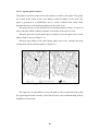
Habitat Monitoring: This is one of the main areas in where Intel Research
Berkley Laboratory and the College of the Atlantic are deploying and using
wireless sensor networks to study the microhabitats on the island of Great
Duck, Maine (North American coast)[9]. This is a project that uses WSN to
monitor underground nests of the storm petrel, a type of seabird, which has
been very difficult to study and whose preferences of living are mainly
12
based on this island. With this, the scientifics will know why this type of
bird prefers this island, if this is associated to the microclimate and all of
that without modifying aggressively the habitat of the bird. For this purpose
it has been introduce a “mote” into the nests and another one outside, 4inches far away, to receive sensing data like temperature, from the
underground mote. The motes outside communicate each other and send the
data retrieved in the motes through the sensor network to a gateway which is
connected to a laptop in the research station, then to a satellite and finally to
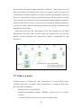
a lab in California (see Figure 2.2). As the biologist Anderson says in [10],
this technology will change the biology forever.
Figure 2.2: Wireless Sensor Network in the Great Duck Island, monitoring the storm
petrel (seabird). From 1 to 5 it indicates the process of transmitting data from the
motes to the gateway and finally to the satellite [10].
-
Environmental Control: In the botanic gardens in Huntington, San Marino
(California), where there are more than fifteen thousand different species of
plants, researches of the Jet Propulsion Laboratory (JPL) of the NASA are
currently working with a web Wireless Sensor Network to controls the
humidity, hot, ground state, … [11]. Every certain time, the sensors update
themselves, sending the information to a gateway that sends the data to the
supervisors.
13
-
Military Surveillance: As it happened with the creation of Internet, the
Defense Advance Research Projects Agency (DARPA) is one of the main
research groups trying to develop this technology. In fact the idea of “smart
dust” was created by a researcher in this agency; it is based on spreading
over the battle field, thousands of sensors which connect wirelessly [12].
These sensors will control the movements of the troops and the enemy
vehicles without warning them. The sensors will form an intelligent, autoorganized network which could retrieve all data and just send the important
data. DARPA is working in collaboration with the University of California,
Berkeley and Intel Company within the Center for Information Technology
Research in the Interest of Society (CITRIS).
-
Medical Monitoring: Intel currently has some lines of research in this field,
for example the creation of centers of medical attention to help patients with
memory problems and alert them to take its medicaments. Motes can be
monitoring vital signs, sending this information through ambulances all over
the city, so the closest one will have information about its patients in an
action radius.
-
Intelligent Building Control: In the design of “intelligent” buildings one of
the main concerns is the sensors network. Often there is not possibility of
installing wired networks in historic buildings, monument and generally
after construction; for this purpose WSN can be installed everywhere nearly
without modifying the environment. Besides sensors in WSN have a more
powerful analysis of the information through the wireless connection so the
flow is faster and the decisions can be taken faster. These sensor offers
information about temperature, humidity, sound, light, presence control,
etc… Moreover, it is being developing GPS indoor systems which allow
mobility of sensors to specific positions to control everything even if the
sensors are not initially positioned properly.
Other interesting areas of applicability are: Security, Inventory Tracking, Smart
Spaces or Traffic Control, but the possibilities are huge.
14
2.6 – NesC and TinyOS
2.6.1- NesC
NesC is a new structured, component-based programming language for networked
embedded systems like Wireless Sensor Networks. NesC has a C-like syntax
(extension to C) designed to embody the structuring concepts and execution model
of TinyOS, the operating system for WSN.
According to [13], these are the basis of NesC:
-
Separation of construction and composition: Programs are built out of
components, which are assembled (“wired”) to form whole programs.
Components define two scopes, one for their specification (containing the
names of their interface instances) and one for their implementation.
-
Specification of component behaviour in terms of set of interfaces:
Interfaces may be provided or used by the component. The provided
interfaces are intended to represent the functionality that the component
provides to its user; the used interfaces represent the functionality the
component needs to perform its job.
-
Interfaces are bidirectional: Interfaces specify a set of functions to be
implemented by the interface’s provider component (commands) and a set to
be implemented by the interface’s user component (events). Interfaces allow
communication between components in the way of a command executing an
action that goes downwards through the components in layers and events
coming upwards in the hierarchy of layers (as a result of a command or an
interruption). For example when a packet is sent with the “send command”
from the SendMsg interface, an event “sendDone” (which must be
implemented in the user component) will be signalled if it has been
successfully sent. This allows a single interface to represent a complex
interaction between components.
15
-
Components are statically linked to each other via their interfaces: This
increases runtime efficiency, encourages robust design, and allows for better
static analysis of programs.
-
NesC is designed under the expectation that code will be generated by
whole-program compilers: Everything will be compiled statically so there
will no be problems like dynamic memory allocation and data race
conditions can be detected (nesC owns a detector). This allows for better
code generation and analysis.
-
The concurrency model of nesC: Is based on run-to-completion tasks,
interrupt handlers which may interrupt tasks and each other and detection of
data races at compile time. Components have internal concurrency in the
form of tasks. Threads of control may pass into a component through its
interfaces. These threads are rooted either in a task or a hardware interrupt.
-
Files for NesC have the extension “.ns” for all type of components.
According to [14] those are the challenges that have to be addressed in this type
of embedded systems (WSN):
-
Driven by interaction with environment: WSN are specific-purpose rather
than general-purpose computing systems, event-driven (reacting to changes
in the environment) rather than driven by interactive or batch processing.
Consequently, events and processing activities need a concurrency model.
-
Limited resources: It considers that motes have very limited physical
resources, because of its characteristics so it has to minimize the use of those
resources doing it efficiently.
16
-
Reliability: It is expected that these systems runs with autonomy for long,
and since there is no real recovery mechanism and fails in hardware can be
expected, reliability has to be guaranteed in the software level.
-
Soft real-time requirements: These type of systems (WSN), although they
can require time critical tasks (radio management or sensor polling), they do
not really need hard real-time guarantees. Timing constraints can be
addressed by having control over the OS and application.
Based on challenges above and after combining properties of different
programming languages, these are the global features of NesC [14]:
-
NesC
integrates
reactivity
to
the
environment,
concurrency
and
communication. As it is oriented to this type of concurrent systems where
resources are limited, it performs whole-program optimizations and
compile-time data race detections to simplify application development,
reduce code size and avoid potential bugs, in order to maximize the
efficiency.
-
Because of the fact that nesC is oriented to systems which are hardly tied to
hardware, all resources are known statically and applications are built from
reusable component libraries. Besides nesC compiler performs static
component
instantiation,
whole-program
inlining,
and
dead-code
elimination.
-
Although function pointers and dynamic memory allocation were prohibited
nesC is capable of supporting complex applications.
-
The design of applications has to be flexible, to easily decompose it and be
able to integrate in different hardware platforms where the boundaries
between hardware/software can vary. NesC provides bidirectional interfaces
to simplify event flow, supports a flexible hardware/software boundary, and
17
admits efficient implementation that avoids virtual functions and dynamic
component creation.
-
NesC defines a simple but expressive concurrency model coupled with
extensive compile time analysis: the nesC compiler detects most data races
at compile time.
-
NesC provides a balance between accurate program analysis to improve
reliability and reduce code size, and expressive power for building real
applications.
Table 2.2: Description of the main TinyOS/nesC components [13]
2.6.2- TinyOS
According to [15], tinyOS is an open-source, component-based, event-driven
operating system designed for wireless embedded sensor networks in which devices
have very limited resources. It has a very small footprint, the core OS requires 400
bytes of code and data memory combined [16]. Actually nesC was designed to
support and evolve TinyOS’s programming model and to re-implement TinyOS in
18
the new language. In fact, nesC was created to suit the needs of TinyOS, so
principles are the same in both nesC and TinyOS.
TinyOS has several important features that influenced nesC’s design [14]:
-
Component-based architecture: TinyOS features a component-based
architecture, which enables rapid innovation and implementation while
minimizing code size as required by the severe memory constraints inherent
in sensor networks. It provides a set of reusable system components in
libraries which includes network protocols, distributed services, sensor
drivers, and data acquisition tools. Components are organized according to
functionality and it is followed a layer architecture (see Figure 2.3). An
application connects components using a wiring specification that is
independent of component implementations. Components can be modules
(implement the behaviour) or configurations (link -wire- components) (see
Table 2.2). Decomposing different OS services into separate components
allows unused services to be excluded from the application.
Figure 2.3: TinyOS component layer architecture [16]
-
Tasks and event-based concurrency: There are two sources of
concurrency in TinyOS: tasks and events.
o Tasks are a deferred computation mechanism. They run to
completion and do not pre-empt each other. Components can post
tasks; the post operation immediately returns, deferring the
19
computation until the scheduler executes the task later. Components
can use tasks when timing requirements are not strict; this includes
nearly all operations except low-level communication. To ensure low
task execution latency, individual tasks must be short; lengthy
operations should be spread across multiple tasks. The lifetime
requirements of sensor networks prohibit heavy computation,
keeping the system reactive.
o Events also run to completion, but may pre-empt the execution of a
task or another event. Events signify either completion of a splitphase operation (discussed below) or an event from the environment
(e.g. message reception or time passing). TinyOS execution is
ultimately driven by events representing hardware interrupts.
Commands and events that are executed as part of a hardware event
handler must be declared with the async keyword.
Because tasks and hardware event handlers may be preempted by other
asynchronous code, nesC programs are susceptible to certain race
conditions.
Races are avoided either by accessing shared data exclusively within
tasks, or by having all accesses within atomic statements.
The nesC compiler reports potential data races to the programmer at
compile-time. It is possible the compiler may report a false positive. In this
case a variable can be declared with the norace keyword.
The simple concurrency model of TinyOS allows high concurrency with
low overhead, in contrast to a thread-based concurrency model
in
which
thread stacks consume precious memory while blocking on a contended
service. However, as in any concurrent system, concurrency and nondeterminism can be the source of complex bugs, including deadlock and data
races.
-
Split-phase operations: As was described for nesC, commands and events
perform operations by splitting responsabilities. Tasks execute non-preemptively so TinyOS has no blocking operations, then the only way to
20
address it is split long-latency operations. “Commands” are typically
requests to execute an operation; if the operation is split-phase, the
command returns immediately and completion will be signalled with an
event. An example is the sending process, a command request the sending of
a message and if it is successful and event is signalled.
Non-split-phase operations like toggle an LED do not have completion
events.
Resource contention is typically handled through explicit rejection of
concurrent requests.
21
Chapter 3 – Ad hoc Routing Protocols
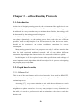
3.1- Introduction
At the time of designing routing protocols, the environment of the application is one
of the main important issues to take in mind. The constraints of the technology must
be addressed in a way or another to try to minimize them. Besides, the topology will
be determined by the routing protocol being used.
In Wireless Sensor Networks where the devices may have mobility, topologies
can change dynamically, so the routing process have to be the most efficient
possible, based on the principles of an ad hoc protocol (if the devices are static,
should not be mandatory), and trying to address constraints like power
consumption.
Many routing protocols have been proposed, not only for ad hoc networks but
also for wired static and traditional networks. All of them address different
constraints, depending on the characteristics of the network to which are applied.
In this chapter it will be explained some of the specifications and workings of
some important routing algorithms which have helped in the process of designing
the proposed project algorithm.
3.2- Graph based routing
3.2.1- Bellman-Ford
This is one of the most famous used in wired networks. It was used in ARPANET,
and it is based on getting the shortest path through a node. The time is the
estimation process.
According [17], every router maintains a table with the best distances to reach
every node and the paths to achieve it. The tables are interchanged between
neighbours to update themselves. For every entry (unique for every destination) in
the table, it is saved the preferred exit and an estimation of the time to reach the
destiny node.
22
Any router have to measure distances with its neighbours depending on the type
of measure being used (eco packets for delay measure).
Every certain period of time the routers interchange its tables with the
neighbours, and with the new tables obtained the router calculates better distances
and updates its table if it finds better routes.
3.2.2- Dijkstra
Edsger Wybe Dijkstra created this algorithm in 1959. This algorithm is used in
finding the shortest path between a node and the rest of the nodes in the network in
TCP/IP networks. Conforming with [17] the estimation is based on a function of
weights. The algorithm has a complexity equal to O (n2) with “n” number of nodes.
This is the way of working.
-
In a graph, every arc between two nodes will have an associated weight.
-
The shortest path to go from a node to another is when the sum of all the
weights of the arcs which form the path is the lowest possible from all the
available paths between the two nodes.
-
It is based on the optimality principle that states: if in the shortest path
between two nodes u and v, there is a node w, the path between w and v
must be the shortest.
-
It uses the already established shortest paths to create other paths, so it takes
profit of the information available in the network.
3.2.3- Min-Hop Algorithm
This is based on the Dijkstra algorithm above. It is based on choosing for the next
hop on the routing process the node which has the less weight. Because of that it is
probably that it is not chosen an optimum path than with the other algorithms. The
problem with this algorithm is the overload of the best links (minimum weight) and
do not take into account the rest nodes for having less quality, that makes a non
efficient and well balanced use of the resources in the network.
23
3.3- Ad Hoc Routing Protocols
The main feature of this type of networks is its dynamicity; all the nodes have
mobility and can leave and enter in new networks at any time so the algorithms
should manage all of that possible failures (fault tolerance).
Another concern that this algorithms should address is the efficient use of the
energy because usually all mobile devices carry its own power system which have a
period or life and mostly the sensors (motes).
Now it will be presented two types of classifications for these types of
algorithms:
3.3.1- Routing classification 1
A general classification for routing protocols is based on the time when the routes
are discovered, statically or on demand [18]:
- Pro-active (Table-Driven Routing)
This type of protocol works out routes in the background independent of traffic
demands. Ever node stores information about the topology of the network in
tables, which are updated every time a new message is received. There is a
process in charged of sending, receiving and analyzing packets to discover the
topology. This information in the tables is then queried to obtain routes to send
data to a node. It is slow to converge and may be prone to routing loops. It keeps
a constant overview of the topology which creates overhead if there is no data to
be sent. This type of algorithm needs resources like power, link bandwidth and
storage capacity so depending on the features of the network it could not be
suitable for ad hoc routing and neither for Wireless Sensor Networks.
Examples of this type of routing algorithms are: FSR, DSDV, WRP, CGSR,
and STAR.
-
Reactive (On Demand Routing)
This type of protocol reacts depending on the need of data being sent. There is
no information in tables on how to reach nodes in the topology. When a node
wants to send data, it ask tables which store already searched routes, if there is
24
no information on how to reach this node, it starts a discovery process. The
discovery process uses different methods to obtain different paths, the most well
known is flooding. Once it is obtained the best route it is saved in the table of
the mote to avoid repeating the discovery process again (out of date routes are
controlled with timestamps). This type of algorithm is very efficient for ad hoc
networks when the route discovery is less frequent than the data transfer. They
are more suited to large networks with light traffic and low mobility.
Examples of algorithms are: DSR, ABR, TORA, AODV, CBRP, and
RDMAR
-
Hybrid (Pro-active/Reactive)
It is combined both pro-active and reactive protocols using distance-vectors for
more accurate metrics to establish the best paths and it react reporting routing
information just when there is a change in the topology of the network. Each
node in the network owns an action radius zone, defined by metrics like number
of hops; the node just keeps information in tables about its zone, minimizing the
content in the tables.
The most well known example is Zone Routing Protocol (ZRP).
3.3.2- Routing classification 2
Classification according to the way the neighbours are searched and the paths are
found:
-
Flooding
A message from a node is sent to all its neighbours and those to its neighbours
too and so on, sending copies of the message to all the nodes in the network,
The problem is the collisions mainly in wide networks, it has to be checked to
avoid cycles (do not send the same message to your neighbours twice). Besides
there is a waste of energy in sending all these messages all through the network
but depending on the use of the message data to update every node, it can be
taken profit from the process.
25
-
Bellman-Ford Algorithm
Although it was described in section 3.2.1 as a non ad hoc algorithm, it can be
applied to ad hoc networks too. The difference will be that all nodes keep
routing tables then all nodes will act as routers. The problem with this algorithm
comes when the networks are too wide, the tables need a lot of entries to be fault
tolerant and the memory in mobility nodes is an important constraint.
-
Gradient Algorithm
According to [19], it is a kind of flooding because the messages are not sent to a
specific node; they are sent to their neighbours. In this algorithm tables with
weights are defined which give information or measure about what route should
be followed. The tables are not transferred through the network. Although the
message is sent to all the networks (act as a routing), each node which receive a
message and will decide consequently so the number of messages being sent
will not increase that much as in flooding (see above).
-
Stigmergy Algorithms (Ant Algorithm)
Based on that [20], this type of algorithms tries to imitate the behaviour of some
colonies-life animals when they have to discover paths to get the best way
through the food, and how they follow each other based on probability and the
modification of the environment. For example in the case of ants, they discover
the optimum path to the food by leaving pheromones in the way. As the shortest
route will contain more concentration of pheromones (more ants will cross the
shortest way faster), all the ants will end up following the most “smelly” path.
At the beginning of the process they apply functions of probability and
pheromone concentration but once the pheromone concentrations starts to get
bigger, the pheromone measure becomes the main estimator to follow the route.
26
3.3.3- OLSR (Optimization Link State Routing) Algorithm
This is a proactive routing protocol, using flooding technique to determine the
topology in the network. The information containing the topology is sent to all the
nodes using flooding which provides available routes quite fast without a huge
overload. The protocol should be independent from the layers above (data-link
layers), that’s why it is based on how to communicate or features of the
communication as estimation of the quality of the link.
These are the three mechanism used in the protocol [21]:
-
Neighbours Discovery Mechanism
The link between a node and a neighbour can have these three states:
-
No link: There is no communication with the neighbour.
-
Symmetric: The communication from the node to the neighbours exists as
well as from the neighbour to the node.
-
Asymmetric: The communication just flow in one direction, from the
neighbour to the node or vice-versa.
To detect neighbours a node transmit periodically HELLO messages, with
information like the address of the node, the list of neighbours and the link state
with them, in order to detect changes in the network.
With this, a node which receives the messages can determine the state of its
neighbourhood as well as the nodes which are 2 hops far it. This information is
stored in each node and has to be saved for a certain time and updated with the
next HELLO messages.
-
Traffic Control Mechanism
With the information of the link state from the neighbours and the nodes 2-hop
far, now it has to be controlled the data flow with which the network will be
flood to discover the topology. This is based in a simple mechanism based on
flooding.
To control the network it is used a flooding control message. When a node
receives this message for the first time, it forwards it to its neighbours. Doing
27
that neighbours will get duplicate messages but it is ensured that the message
will be received by all nodes.
Collisions will be a problem with the messages from the nearest nodes so the
algorithm defines the Multipoint Relay (MPR), which are nodes selected to send
the messages to the node 2-hop far away. These nodes must have symmetric link
with the source node. The way of selecting this type of nodes depends on how
they will be used, taking into account the minimum number of nodes needed to
retransmit a message 2 hop distance.
To control the flooding process of these messages, these rules have to be
followed:
-
The message should have the intention of being forwarded.
-
The message must not have been received by the node previously.
-
The message received must come from a node selected as a MPR.
-
Routing Mechanism
In order to route the data over the network every node has to get the information
about all nodes in the network. To do that it is used the Topology Control (TC)
messages, which contain the source address and the address from the MPR’s.
These messages are sent by the nodes which own a MPR. The purpose of these
messages is to advertise what connectivity has the MPR, so the nodes will
receive a graph with partial information about the network topology. This
information is enough to apply an algorithm to select the shortest path. This
information will be valid for a period of time until it is updated.
3.3.4- Direct Diffusion Algorithm
It is based on data-centric routing and it is very lean to sensor networks. The
purpose of the algorithm [22] is the diffusion of data through sensor nodes by using
a naming schema for the data, in order to avoid unnecessary operations of network
layer routing to save energy.
It uses attribute-value pairs for data and the sink queries the sensors in an on
demand basis. To create a query an interest is defined using a list of attribute-value
pairs such name of objects, interval, duration, geographical area, etc. The interest is
28
broadcasted by the sink to all of the nodes in the network which stores the interests
to compare them later with the data received and decide where to route. The interest
entry also contains gradient fields and it is used both of them to create the paths
between sink and sources. The gradients are very useful to determine quality of
paths, as they are reply links to neighbours, from which the interest came from,
containing data rate, duration and expiration time.
As many paths can be established in the process, the path is selected by
reinforcement with the sink resending the original interest through the path with a
small interval forcing the source node to send data more frequently. A very
interesting feature of Direct Diffusion is the re-identification of a new route among
the other possible paths in the event of an already established path fails, by
reinitiating the reinforcement process. Multiple selected paths can be previously
selected to save energy cost in the process of reinforcement but there will be extra
overheads of keeping those paths.
There is no need for addressing mechanism as it is data centric with
communication neighbour to neighbour, each node can aggregate data and there is
no need to maintain global network topology.
Because of the fact that the algorithm is based on a query-driven on demand
model, applications which require continuing monitoring from sensors to the sink
will not work efficiently.
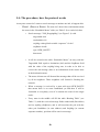
3.3.5- Rumor-based Algorithm
The idea of this type of routing is the use of “agents”, to create the paths through the
network to the events when they happen [23]. Agents are messages with expiring
time which travel over the network. After the agents generate these paths the
“queries” are routed following them. Firstly the queries are sent by a random path.
Each node in the network keeps a neighbour table and another table for events that
contain the information of the expeditions which have gone through it. At the
beginning, lists of neighbours are generated broadcasting each node’s identification.
When the events have a limited life time, timestamps can be used in the events
tables.
29
3.3.5.1- Agents (path creators)
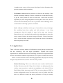
The paths are stored as states in the nodes and are created by the agents. The agents
are created in the nodes of the event adding a path of length 0 to the event. The
agent is generated in a probabilistic way to avoid overhead when many nodes
generate the same event and many paths go to the same event.
The agent travels over the network for a maximum number of hops. It carries its
own event table which combines with the event tables of the nodes it visits.
When an agent cross a path which goes to another event, the agent start to create
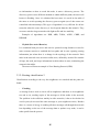
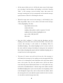
paths to both events (see Figure 3.2).
When an agent finds a node with a longer path to the event, it updates the node
routing table with the shortest path (see Figure3.1).
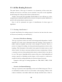
Figure 3.1: The agent modifies the exist path to a more optimal one [23]
The agent uses an algorithm to correct the path in order to generate better paths
by registering the nodes recently visited (avoid cycles) and communicating with its
neighbours in each node.
30
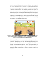
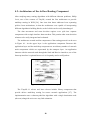
Figure 3.2: When agent prorogation the path to Event 2 comes across a path to Event
1, it begins to propagate the aggregate path to both [23]
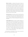
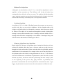
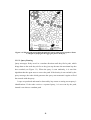
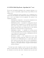
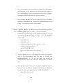
3.3.5.2- Query Routing
Query messages firstly travel in a random direction until they find a path, which
brings them to the node they ask for or they just stop because the maximum hop has
been reached (see Figure 3.3). When the query is sent randomly, it is used the
algorithm that the agent uses to correct the path. If the destiny is not reached by the
query message, the node which generates the query can retransmit it again or flood
the network with the query.
Loops are produced and must be detected by hop count or storing recent query’s
identifications. If the node receives a repeated query, it is not sent by the path;
instead it can choose a random path.
31
Figure 3.3: Query is originated from the query source and searches for a path to the
event. As soon as it finds a node on the path, it’s routed directly to the event [23]
3.4- Link State Estimation
There are many different systems to estimate the link state, systems which performs
great in wired networks and which can not be used in wireless because of the
complete different principles in communication between nodes. Wireless systems
are driven by failures in communication; the transmission mean is less reliable so
the metrics for evaluation which includes agility, stability and amount of history
required for estimator, have to be well tuned according to the constraints of the
wireless network.
For the purposes of Wireless Sensor Networks, it has been evaluated several
estimators as in [24]; the most significant and successful will be described in this
section.
3.4.1- EWMA (Exponentially Weighted Moving Average)
This estimator is very simple, widely used and memory efficient but it requires
constant storage for history tuning.
It is reactive to small shifts, often used in statistical process control applications
detection because of its agility. It is based on a linear combination of infinite
32
history, weighted exponentially, updating the history with packets received
successfully according to a time interval which is suppose to be the time in between
the reception of two consecutive packets; with the time interval, which has to be
tuned, it can be calculated how many packets were lost and make the calculations
for the estimation.
The implementation of EWMA will take 4 bytes (floating point) or 1 byte (fixed
point) to store the current estimation with just 2 multiplications and 1 addition
involved in the computational process.
The process of tuning [24] indicates that in order to keep the estimation within a
10% error, the agility has to be sacrificed. On the other hand if it is tuned to
provides agility, good for detecting disappearance of neighbour nodes over a
relatively short time, the estimation will not be very useful because of the large
overshoots and undershoots (sensitive to small shifts). Besides, it was measured that
the crossing time for EWMA is 167 packets while settling time is close to 180
packets.
3.4.2- Flip-Flop EWMA
As it was described above, it is quite difficult to provide both agility and stability in
the same estimator, because of that it is proposed a flip-flop between two EWMA
estimators which implement stability and agility features.
In [24], this approach was tested; the switching between agile and stable
estimators was produced when the difference in deviation was greater than 10%. On
the other hand if the estimator by default was stability, it changes to the agile
estimator when it can be detected sudden changes such as mobility much earlier. It
was shown in [19, 24] that the flip-flop does not provide advantage over EWMA,
but it could be caused because of the switching threshold.
3.4.3- WMEWMA (Windows Mean EWMA)
It uses the average of a time window to adjust the estimation using the latest
average which is actually an observation of the estimation. EWMA then is applied
to filter more the estimation. It is based on messages received and sum of losses to
calculate a mean in which is involved 2 additions, 1 division and two
33
multiplications as computational operations, saving the result in 1 byte (fixed point)
or 4 bytes (floating point), same as in EWMA, but with the different of using 2
bytes to store the number of messages received and looses. The computation is done
in function of the time window instead of every certain time event.
According to [24], the observed settling time and crossing time is relatively
small, the fastest of all studied but as EWMA is sensitive in the agile scenario there
is not significant improvement.
34
Chapter 4: Routing in TinyOS
4.1- Introduction
The process of routing in Wireless Sensor Networks is based on that of ad hoc
routing protocols which can support the mobility of motes (nodes). The nature and
novelty of WSNs, together with the difficulty of debugging make direct
implementation extremely challenging [25]; therefore most of the current ad hoc
algorithms have only been tested in simulators, but not on real motes.
The main objective in routing is to carry information from the motes to the root
mote or base mote, which is then connected through a gateway to a computer which
can analyze, transform or publish the data.
The main objective in ad hoc routing protocol design is to have the motes acting
as data retrieval devices, directing this information through a root mote for late data
analysis. Two topologies have been used to classify the networks and hence in the
design of new ad hoc protocols; these topologies are: tree-based and cluster-based.
Because of the nature of the monitoring process WSNs fit perfectly into these
systems and hence allow the designers of new ad hoc algorithms to address
constraints such as minimizing the number of communication messages being sent,
leading to a reduction in power consumption by the motes.
In this chapter the routing process in TinyOS will be detailed. As discussed
previously many different versions of TinyOS exist; in this chapter the routing
system used in all versions within 1.x. will be detailed. This type of routing is based
on a hierarchal topology like the tree-based topology.
Overview of the new algorithms provided with more recent releases of TinyOS,
v2.0. will be described. Two new ad hoc routing algorithms have been produced:
one of them is based on data aggregation while the other is concerned about
dissemination of routing data over the network. Hence although the hierarchy is
maintained, both routing directions can be taken, i.e. to and from the root mote.
35
4.2- Architecture of the Ad hoc Routing Component
After studying many routing algorithms with different inherent problems, Philip
Levis, one of the creators of TinyOS, created the first architecture to provide
multihop routing in WSN [26]. One issue that theses addressed was separating
policies from mechanisms; in that the architecture was capable of incorporating
different algorithmic building blocks, each of which can be easily interchanged.
The data movement and route decision engines were split into separate
components with a single interface between them. This permits other route-decision
schemes to be easily integrated and evaluated.
The architecture created and the components of the routing protocol can be seen
in Figure 4.1. At the upper layer is the application component. Between this
application layer and the multi-hop component are an arbitrary number of network
stack components which are represented by the transport layer. An application
interacts with the network stack through the Send and Receive interfaces; use of the
Intercept interface is optional however it is frequently used to sniff packets.
Figure 4.1: Component Architecture [26]
The TinyOS-1.1 release and later releases include library components that
provide ad-hoc multi-hop routing for sensor network applications [27]. The
implementation uses a shortest-path-first algorithm with a single destination node
(the root) alongside active two-way link estimation.
36
4.3- EWMA Multi Hop Router Algorithm (the 1st one)
This was the first algorithm implemented with a component architecture as in
Figure 4.1. It uses an exponentially weighted moving average (EWMA) for link
estimation [24].
As for all the applications written for TinyOS it uses a configuration file to
connect (wire) the components and establish which interfaces are provided and
used, as well as the modules of the new application. The structure of the
components is as follows:
-
MultiHopRouter (configuration) - is the top-level configuration for the
routing layer, which wires (connects) the next modules.
-
MultiHopSend (module) - is responsible for sending packets using the
implemented ad-hoc routing protocol. It is responsible for decisions like
when and how many times to retransmit and when alternate parents
should be requested. When a new message needs to be sent it calls the
RouteSelector component interfaces to prepare the package.
-
MultiHopRoute (module) - is responsible for receiving protocol
messages and deciding whether it should forward them. If a message has
to be forwarded then it passes the packet to MultiHopSend which will
call RouteSelector to prepare the packet.
-
RouteSelector (module) - is the component that can be easily
interchanged. It maintains routing state, which it uses to choose routes
for packets to send. MultiHopSend passes it a packet buffer, which it
fills in with the necessary header fields to be used by MultiHopRoute.
This is the component that makes the decisions of routing based on
estimators (e.g. Link Quality Estimator, Geographic Position Estimator,
and Power Estimator).
The nodes keep a table of neighbour in order to keep track of the neighbours
which are accessible within one radio hop. The information in the table is based on
the information received from other nodes. Information about the parent (node
37
through which it arrives to the root) is stored and is based on ack/nacks that the
parent sends.
The estimation technique in EWMA is based on the link state; a better
description can be found in Chapter 3.
The success in receiving packets is calculated by the difference in the sequence
number, so the reception of messages has to be an small multiple of the time
interval, otherwise the failure is based on an accumulation of a silent count where
there is no reception.
The ack received from the parent is used to increase the value of this node as the
parent, in comparison with the rest of the neighbors.
4.4- WMEWMA Multi Hop Router Algorithm (the 2nd one)
The second version of the algorithm follows the same architecture of that outlined
above, for version 1.x of TinyOS. The difference with respect to its predecessor is
that the link estimator measure is based on WMEWMA (Window Mean with
EWMA) which offers more efficiency and simplicity [28].
According to [27], the configuration which wires (connects) the new
components is given in Figure 4.2; the direction of arrows indicates interface
provider/user relationships, not data flow direction.
Figure 4.2: MultiHopRouter configuration [27]
38
Applications should maintain an average message frequency at or below one
message every 2 seconds. Higher rates can lead to congestion and or overflow of the
communication queue.
4.4.1- Interface Description
The component configuration provides 6 interfaces. A '[ ]' after the interface name
indicates the interface is parameterized and it can contains any type of AM
messages defined in an “.h” file.
-
StdControl - The standard control interface
-
RouteControl - A special interface for controlling monitoring router operation. This is the interface called to obtain the route to the parent.
-
Receive[] - In this implementation, the base station is the only implicit
destination for packets, as it is the sink in the topology. This interface
exists only as a stub and is not implemented.
-
Send[] - The port to use for locally originated packets.
-
Intercept[] - This port is used when a packet is received that will be
forwarded. It provides a means for an application to examine forwarded
traffic and, depending on the value returned, suppress the forwarding
operation in order to control cycles.
-
Snoop[] - The Snoop port uses the 'Intercept' interface definition, but
with different semantics. It is signaled when a packet is received that
will not be forwarded. This interface is useful for passive monitoring of
traffic for replication purposes.
4.4.2- Component Description
The components have changed relative to the previous version but the architecture
schema has been maintained. The configuration file is the same but has internal
code to multiplex between the two versions (different names and new interfaces).
These are the configuration file and the modules:
-
MultiHopRouter - This configuration connects MultiHopEngineM,
MultiHopLEPSM with other necessary components (queueSend, comm,
39
timer…) which are more primitive components used to access the low
layers in the architecture. These are the main tasks of this configuration
file:
o Exports the Receive, Send, Intercept and Snoop ports to
applications.
o SendMsg port of MultiHopEngineM is wired (connected)
to the QueuedSend library components for queuing
outbound packets (both forwarded and locally originated).
o ReceiveMsg and SendMsg ports of MultiHopLEPSM are
wired
(connected)
to
the
AM_MULTIHOPMSG
parameter of the communication provider for the purpose
of exchanging single-hop route updates with neighbors.
-
MultiHopEngineM - Provides the overall packet movement logic for
multi-hop functionality. It only requires that the RouteSelect and
RouteControl interfaces be available.
o Using the RouteSelect interface, it determines the nexthop path and forwards the packets out the parameterized
SendMsg port.
-
MultiHopLEPSM - Provides the Link Estimation and Parent Selection
(LEPS) mechanisms for the multi-hop implementation.
o It monitors all traffic received at the node via the Snoop
port.
o It directly receives single-hop route update messages
(AM_MULTIHOPMSG) that may be sent from neighbors
within the single hop range.
o The
module
internally
sends
and
receives
AM_MULTIHOPMSG messages to manage the nearest
available neighbors and it decides the next hop
destination based on shortest path semantics.
o The root node (address=0) or sink is discovered based on
the minimum number of forwarding messages.
o By default, the module sends a route update message once
every 20 seconds and re-computes after 50 seconds (5
route update messages).
40
o The flexibility in this module is so high that it can be
replaced for another one, just following the same
convention names and parameters within the interfaces.
Thus new estimation measures can be inserted into the
routing layer for evaluating. For example, a min-hop
algorithm might have an estimator that listens for protocol
messages and updates routing tables accordingly.
4.5- Structure of the multihop message
In this section we describe the structure of the message that implements the routing
logic of the protocol (see Figure 4.3). All messages must be parameterised by an
uint8_t id which identifies the type of messages the interfaces are handling, in this
case the id number is 250. As this message will be encapsulated in the data field of a
standard sending message TOS_Msg (see Figure 4.4), it has the same length of the
data field, 29 bytes. 2 bytes are used for keeping the source address of the sending
message, another 2 bytes are used to store the original address of the data being
sent, another 2 bytes are used for the control sequence field and a last control field
contains 1 byte and is used to store the number of hops the packet has been carried
so far. The type of message being sent by any application must fit into 22 bytes (297 bytes). So it can be seen that many different type of messages may be sent in the
base message using the structure based on the data field as a nested link. Because of
this the interfaces are often parameterized to allow for easy identification of the type
of message being sent and to allow the bytes with the appropriate message struct
type.
enum {
AM_MULTIHOPMSG = 250
};
typedef struct MultihopMsg {
uint16_t sourceaddr;
uint16_t originaddr;
int16_t seqno;
uint8_t hopcount;
uint8_t data[(TOSH_DATA_LENGTH - 7)];
} __attribute__ ((packed)) TOS_MHopMsg;
Figure 4.3: AM_MULTIHOP message structure
41
typedef struct TOS_Msg {
uint16_t addr;
uint8_t type;
int8_t group;
int8_t length;
int8_t data[TOSH_DATA_LENGTH];
uint16_t crc;
} TOS_Msg;
Figure 4.4: TOS_Msg message structure
4.6- Sending a packet
The use of the multi-hop library component is mostly transparent to the application,
in so far as the application uses the Send interface to connect to the mutihop
component to achieve multi-hop functionality.
When an application wants to send a packet of a defined type (struct):
-
First of all it should call the Send’s interface getBuffer command to
obtain a pointer to the data region of a mutihop packet, where the data
will be nested for transmission. This call allows interface users to remain
unaware of the packet format used by the provider. Once the command
getBuffer is called, it will automatically initialize the protocol fields to
state that the mote is the source for the packet.
-
Once the pointer is obtained, interface MultiHopRoute will provide
information about routing, e.g. the parent, hops… that can be added to
the appropriate field of the message.
-
Finally the TOS_Msg buffer, where you get the pointer to the field data
within an already nested multihop message, it should be called using the
Send interface’s send command. This send command is wired
(connected) to its equivalent in the MultiHopRoute configuration to
provide multihop functionality.
42
4.7- Receiving a packet
To receive packets from a specified id type in an application, the event
Receive.receive, with the parameter [uint8_t] specifying the type of message it is
desired to receive, must be declared. The multihop components will then signal the
event through to the application layer if the message is from this type and the packet
is destined for this mote. Internally the reception of an AM message signals
MultiHopRoute which determines if the packet is destined for the local node. If so,
it
signals
MultiHopRouter’s
Receive
interface,
otherwise
it
signals
MultiHopRouter’s Intercept interface, which will generally forward the packets.
To forward the packet, MultiHopRoute calls Send.send on MultiHopSend, using
the same sending policy as if it was the packet originator.
4.8- Other Routing Component Projects
Many other different ad hoc protocols have been developed following the
architecture provided. Usually these change the module MultiHopLEPS for a new
one with a different estimation technique, e.g. based on power consumption [29],
other types of link estimation [30], based on hop count, etc.
A functionality that was not implemented initially in the first routing schema
was the aggregation of data. Here, data received from a child mote in the hierarchy
is aggregated into a data packet to be sent up through the topology to the root. This
technique, explained in detail in [31] produces a considerable reduction in the
number of packets being sent, getting more efficiency from the topology and
consequently reducing the power consumption.
4.9- New Recently Released Routing Algorithms (TinyOS
v2.0)
New protocols have been created to address some of the main constraints or
demands in the routing process. These were released in TinyOS version 2.x on July
2006, so they are in beta release and so not completely tested, or not 100% reliable.
43
All components in both protocols follow the architecture (interfaces, component
structure…). The algorithms have different purpose based on the need in WSNs of
routing data, and both are ad hoc protocols.
4.9.1- Collection
This is based on the main requirement in WSN of collecting data at the base root as
the only sink node for data, using topologies based on trees, sending the data
through the nodes to the root. As the nodes will act as routers, they will inspect all
the packets received so depending on the purpose of the application it will be able to
gather statistics, compute aggregates, or suppress redundant transmissions.
Besides, Collection works with forests of trees: more than one base station can
be picked to receive data; every node will pick a parent and implicitly will join one
of those base stations.
It is a any-cast protocol; it provides a best-effort, multihop delivery of packets to
one of those trees. As it is stated in [32], given the limited state information that
nodes can store and a general need for distributed tree building algorithms, simple
collection protocols encounter several challenges which represent a subset of
common networking algorithmic edge cases that occur in this protocol family:
-
Loop detection
-
Duplicate suppression
(detecting and
dealing with
when
lost
acknowledgments)
-
Link estimation (evaluating the link quality to single-hop neighbors).
-
Self-interference, preventing forwarding packets along the route from
introducing interference for subsequent packets.
The new components implementation and logic can be found at its own section
at [32]; as it can be seen, the components match the previous version ones but with
different functionality.
44
4.9.2- Dissemination
This protocol has a complete different approach to the routing process than
Collection; it is based on the data being routed from the base mote through the rest
of the motes. With that it is intended to make the administrators task of reconfigure,
query or reprogram easier.
Concerning reliability, this new protocol is much more robust to temporary
disconnections or high packet loss; it achieves that by using a continuous approach
that can detect when a node is missing the data (that doesn’t occur on flooding
protocols).
According to the dissemination section et al [32], the dissemination protocol can
vary in efficiency depending on the data size being sent; although the control traffic
protocol part tends to be the same or similar, the data traffic protocol part depends a
lot in the size of data. On the other hand, having a good reliably disseminate
protocol based on small values (quite efficient) is enough to cope with the interests
of the administrators, taking into account the limited memory resources of TinyOS.
Finally, it has to be commented that this new protocol works with versioning in
the event of failure, so the last version it will be the only one seen (although it has
been missed some versions with the failure).
The new components implementation and logic can be found at its own section
at [32]. It doesn’t follow the previous architecture; even the interfaces have not the
same logic; now the paradigm is based on producers and consumers of the data.
45
Chapter 5: Hopping - A bidirectional stigmergy
power efficient on-demand driven ad hoc
routing protocol
5.1- Constraints to address in Routing on SensorNet
Because of the nature of the motes in SensorNet, there are some issues to keep in
mind at the time of designing an ad hoc protocol. Those issues are based on the
deficiencies and differences between the wiring powered connected systems and
wireless battery dependent ones.
The set of devices, “motes”, which communicates via radio (wireless) are
limited in memory resources (ROM and RAM) and powered by batteries (AA)
which have limited life time (6 months to a year). Besides it has been shown in [33]
that the cost in battery of sending a message by a mote is equivalent to calculate
thousands of operations.
Having this situation, it has been studied the actual protocol in charged of
multihop in SensorNet, for the versions 1.x of the TinyOS as it can be seeing in
chapter 4. This protocol works in one direction, sending information from the motes
to the base mote, which is the responsible to process the information from each
mote. It is based on a tree structure where the root (base mote connected to pc) is
the end point and all the rest of the motes use their neighbors to reach it.
Because of that, I believe it will be of great interest and useful application, to
create a protocol which communicates among all nodes without hierarchy that even
could let a set of motes being independent from the base mote (not connected to any
pc), to form self-managed colonies for the purpose of monitoring and controlling .
Furthermore, the reduction of the number of messages being sent among motes
it is a goal that will increase the life of the motes. To achieve this goal, and reduce
the number of messages generated by the motes (broadcast packets sent every 20
seconds in the actual configuration), it will be changed, in the ad hoc paradigm,
46
from a proactive protocol to a reactive one, where the route will be discovered upon
demand.
5.2- The protocol basis
Once studied all the SensorNet architecture, the behavior of the motes, the
unidirectional / bidirectional feature in the communication between motes (a mote
can reach another mote sending but not be reached by this mote), the type, structure
and size of the messages being sent, the memory available in each mote and all
different characteristics of the system, this is the proposed algorithm:
-
All nodes will have the same status and hierarchy and they will be well
defined by an exclusive id mote for each group (example 0x7e).
-
All motes will contain a global counter, “sequence message number” and
it will be increased with every message sent (not forwarded, except in
route discovery).
-
There will be two tables for every mote (see Table 5.1 and 5.2).
Reachable Motes
TargetAddr
SendMote/SeqRoute
0x20
0x12/0x125
Table 5.1: Reachable Motes
Routing Table
RecvMote/SeqRoute SendMote/SeqRoute Usage
o0x4/0x23
0x6/0x56
15
Table 5.2: Routing Table
o TargetAddr= Mote address to be reached from this mote.
o SendMote/SeqRoute= Pair “mote address” and “sequence number”
which create a unique identifier that indicates that in order to reach
the TargetAddr mote, the message has to be delivered to the mote
SendMote with this SeqRoute number.
o RecvMote/SeqRoute= Pair “mote address” and “sequence number”
which create a unique identifier that the messages, which come from
47
the RecvMote with this SeqRoute, have to be sent to the mote
SendMote with SeqRoute in order to reach node TargetNode.
o Usage= It is a number that is set to 1 every time a route is created
and that is increased every time this route is used; this is the indicator
to know which routes are not valid anymore or not used, in order to
improve the search process, otherwise the table will grow up with no
useful entries.
-
An important thing to take into account is that the size of the sequences
“seqmsg” and “seqroute” is an int16_t, that will allow a value of 2exp16=065535; once a mote reaches this number of messages sent, the solutions
would be:
o
It will be sent a flood message to alert all the motes to reset all its
counters and start again (start routing process in all motes). All the
tables in all the motes will be deleted and the global variable
sequence will be set to 0.
o Another solution will be the update of sequence route numbers with
new sequence numbers that will renovate the old sequence numbers
guaranteeing that there will be always a distance between the oldest
sequence number and the most new number generated avoiding
collisions of repeated sequence numbers for a node, even if the
counter of the mote is reset to 0. By the time the mote is reset to 0,
all the old sequence numbers that form routes will be replaced by far
distance numbers within the cycle 0-65536. Those sequence update
messages will be generated based on a timer or even better based on
the number of message, for example every 500 messages, so it will
be guaranteed a minimum distance of 500. The potential problem
that has to be measured is that the cost in sending all of these update
messages can be higher than the cost of starting the discovery route
process again every 65536 messages of the first mote which reach it.
Besides sequence numbers in all the tables will have to be updated
and if the table gets bigger that could delay the routing.
-
It could be thought that routes can change dynamically fast, and better routes
can be found, but although that is true, as long as the first route is found and
48
keeps acknowledging, that will show the route is working and the motes are
not moving so much, so the route could not be the best but the difference in
time, that will be minimum between routes (because of the action radios),
will be coped with the save in number of messages sent to look for a new
one.
5.3- Hopping AM message structure
For the purpose of the multihop message, it will be used the structure in Figure 5.1
where the data field will contain the structure of the application message which
actually carries the data being sent. Then, the multihop message, which will be
called “MHoppingMsg”, will be used to transport the type of message the user is
using in the application. The MHoppingMsg will also be nested in the data field of
the TOS_Msg structure to be transported. The AM id type to identify the type of
message is assigned to id 249 although it could be used the id 250 from the
AM_MULTIHOPMSG, because both algorithms are created from the same purpose
so it will not produce collisions with any other application layer id’s. As it can be
seeing in Figure 5.1, the data field with this type of message will have a capacity of
TOSH_DATA_LENGTH(29) – 9, 20 bytes to store any application message that
has to be transported.
enum {
AM_HOPPINGMSG = 249
};
typedef struct HoppingMsg {
uint16_t targetAddr; //final destination mote for the msg
uint16_t senderAddr; //mote which sends the msg each time
int16_t seqMsg;
//seq of the message (generated by the origin mote)
int16_t seqRoute;
//num seq for route of the mote sending
int8_t type;
//type of msg being sent:
- NEW_ROUTE
- ACK_NEW_ROUTE
- FOLLOW_ROUTE
- ACK_FOLLOW_ROUTE
uint8_t data[(TOSH_DATA_LENGTH - 9)]; //any type of msg being sent
} __attribute__ ((packed)) TOS_HoppingMsg;
Figure 5.1: AM_HOPPINGMSG message structure
49
5.4- The procedure, how the protocol works
At any time a mote 0x3 wants to send a message to another one 0x8, it happens this:
-
Phase1 (Discover Route): The mote 0x3 doesn’t have information about
the route in the “Reachable Motes” table (see Table 5.2) to reach 0x8, then:
o Send a message “TOS_HoppingMsg” (see Figure 5.1) with:
targetAddr=0x8
senderAddr=0x3
seqMsg=value global variable “sequence” for 0x3
seqRoute=0/null
type=NEW_ROUTE
data=none
o It will be created in the table “Reachable Motes” an entry with the
TargetAddr field equal to destination (0x8) and the SeqRoute field
with the value of the seqMsg being sent, in order to be able to
receive the ack message (there is no information of the source mote
in the destination mote).
o The motes in between will forward the message that will be received
by all its neighbors. Those neighbors will forward it flooding the
network.
o When a message is received by a mote with type=NEW_ROUTE
that means there is no route established yet and then it will be
forwarded to everybody (even if it contains the route for the target
node).
o Every mote in the middle will fill the table “Routing Table” (see
Table 5.1) with the received message fields senderAddr (RecvMote)
and its seqMsg (SeqRoute), and it will associate the pair with the
other pair SendMote (its own address) and SeqMsg (its current
sequence number), pair that will be sent in a message.
50
o All the motes which receive it will do the same except for the target
one, checking if the RecvMote and SeqMsg, in the table “Routing
Table”, of the message received already exists; that means the
message is turning into cycles (consequently no forward the message
again) because of the fact of flooding the network.
o When the target mote receives the message, it will identify by the
field “targetAddr” that it is for it, then it will send an ack message
“TOS_HoppingMsg” like this:
targetAddr=null (no info)
senderAddr=0x8
seqMsg=value global variable “sequence” for 0x8
seqRoute=ReceiveMote/SeqMsgReceived
type=ACK_NEW_ROUTE
data=none
o Now the field “seqRoute” is filled with the RecvMote and the
SeqMsg (received) and sent to the mote RecvMote. Once the mote
receives this message it will search in its Routing Table for
SendMote/SeqMsg = RecvMote/SeqMsgd and if it exists it will do
the same with the message forwarding it setting now the associated
ReceiveMote/SeqMsg that match with the SendMote/SeqMsg and so
on until it arrives to the origin mote.
o The mote 0x3 (source one) will wait for an ack of the message; it
will identify the message by the seqMsg, not by the targetAddr field,
as there is no information in the destination node (0x8) about which
mote is the sender. The first ack which arrives will be the fastest
route that will possess bidirectional feature so it will update the entry
in the table “Reachable Motes” with the target mote address and the
SendMote/SeqMsg that it just received (that is the beginning of the
route through the target mote, and it will provide the address where
the message has to be sent and the sequence number for the next time
it is needed to reach this target mote 0x8).
51
o If no ack messages are received after a certain time (that will be
controlled with a timer based on trials, maximums and number of
motes in the network), then a reported error will be passed to the user
application alerting the destination can not be reached.
o For every ack message received in each mote (even if it will be
forwarded), then assumes the route has been established and the field
“Usage” in the “Routing Table” will be set to 0.
-
Phase 2 (Follow Route): The mote 0x3 have information about the route
in the “Reachable Motes” table (see Table 5.1) to reach 0x8, then:
o Look for the target mote, get the pair SendMote/SeqRoute, and send
a message TOS_MHoppingMsg (see Figure 5.1) to the SendMote
address with:
targetAddr=0x8
senderAddr=0x3
seqMsg=value global variable “sequence” for 0x3
seqRoute= SeqRoute (send)
type=FOLLOW_ROUTE
data= nested data from the user message
o The mote which receives it will identify the fields of the message
with its RecvMote/SeqRoute and will find its forward pair
SendMote/SeqRoute. It will fill the fields and forward it,
incrementing the Usage field in the table “Routing Table” (see Table
5.2).
o When it arrives to the target mote (check the targetAddr field) the
reverse process will be done, sending an ack message to identify the
message has been received and the route is still valid, like this:
targetAddr=null (no info)
52
senderAddr=0x8
seqMsg=value global variable “sequence” for 0x8
seqRoute= SeqRoute (received)
type=ACK_FOLLOW_ROUTE
data= none
o The source mote waits for the ack an established time; it checks the
seqMsg & senderAddr fields to verify the ack is for the mote because
of the lack of information in the targetAddr field.
o If there is no ack from the message sent through the pair
SendMote/SeqRoute for the source mote after a certain time (timer)
then it will start the discovery process above.
-
Phase 3 (Garbage Collector): This phase is oriented to eliminate the non
valid routes on the “Routing Table”, routes which are not used anymore or
routes which were created but not used ever because they were not fast
enough. This process will keep the table at the minimum size possible in
order to optimize searches, and consequently increase the routing speed.
o Every certain number of messages received (forward), or when the
size of the table is more than a certain threshold, the table will be
searched and entries with the field Usage set to 0 will be deleted.
o The table then will be sorted by Usage field in decreasing mode to
keep the most frequently used routes the first entries.
o All this process will be performed as an atomic operation to avoid
concurrency problems, so the messages being received will be
queued until the process finishes.
o Timestamp could be used as another field in the table to delete non
recently used routes but instead of that, every fixed interval time the
Usage field will be decreased in 1 unit, so that will guarantee all the
routes non being frequently used to reach the 0 value and be deleted
in the next garbage process.
53
5.5- Features and drawbacks of the protocol
-
The protocol could be improved adding more knowledge of the network to
the motes in between a route, creating sub-routes when the acks arrives to
each mote, creating entries in the table Reachable Motes (see Table 5.1) of
these motes to reach the mote being requested. It has not be created in this
first version of the protocol because it is thought there will be motes which
will act just as routers, then the “Reachable Motes” table will be not useful
and the memory will be wasted.
-
Depending on the nature of the network, the new protocol will be more
successful than the one implemented now in the TinyOS v1.x, but it will
depend on factors like mobility of the nodes and number of messages being
sent per time unit. As soon as the motes moves changing its action radio at a
speed of less than 40 seconds, leaving neighbour radios, the number of
messages will increase due to the need of looking for a new route in every
message trying to be sent ad not receive and ack message.
-
According to the characteristics of the application to be developed one of
both multihop protocols could be used, multiplexing them or even a
combination of both (hybrid protocol) could be created.
-
The lack of information of the source node address in the destination node
can be solved by inserting a new field in the structure of the
“TOS_HoppingMsg” message (see Figure 5.1), like “int16_t sourceAddr” or
the address from the source node can be nested in the data field, in the
structure of the user message; the insertion of the source address as a field of
the user structure message will be a requirement at the time of using the
Hopping Multihop component.
54
Chapter 6 – Developing the protocol on
Wireless Sensor Networks
6.1- Introduction
Although there are more technologies and developers of wireless sensor networks,
the most well known and pioneer institution working on that is the TinyOS Intel
Berkeley group, developers of the TinyOS operating system [2]. They are in close
collaboration with the company Crossbow Technologies [3] which is producing a
big diversity of devices like motes, gateways… and uses TinyOS to create its own
applications.
For the purposes of this project it has been used TinyOS as the operating system,
nesC as its associated programming language and hardware devices from Crossbow
Technologies (motes, sensors and programming boards).
In this section it will be presented the hardware and software used, as well as the
steps to start up from the first approach to WSN to the process of implementing the
protocol. Besides it will be commented the difficulties or typical problems which
appeared. It is believed that this chapter is a good starting point for anyone in this
technology.
6.2- Hardware
6.2.1- Motes
For the purpose of this research it has been used 7 MICA2 motes from the company
Crossbow Technologies [3]. This company produces wide range of sensing devices
In figure 6.1, it can be seen a MICA2 mote. It is composed by a board where it is
integrated the connectors, processor, leds, memory components, switches, radio
devices and a big unit connected to the board where it is placed 2 AA batteries
which provide the power.
55
Figure 6.1: Left: Photo of a MICA2 (MPR4x0) without an antenna. Right: Top and
plan views showing the dimensions and hole locations of the MICA2 PCB without the
battery pack. [34]
The processor in MICA2 mote [35] is the Atmel ATmega 128L low power
microcontroller. It has two modes of processing: active mode where its current draw
is 8mA and sleep mode with 15µA.
In sleep mode MICA2 motes are expected to have a battery life of over 1 year
with the 2 AA batteries. On the other hand, in active processor it depends on the
processing operations, message sending rate but usually it reduces the lifetime
exponentially.
Considering memory specifications (see Table 6.1) the MICA2 mote is
characterized by a Program Flash Memory of 128Kb, where the applications are
stored, another memory module of 512 Kb (flash data logger) that it is usually used
to save sensor data and finally a 4 Kb SRAM memory for execution purposes.
56
Table 6.1: Mote Specifications Summary [34]
Communication in the MICA2 mote is leaded by a max. data rate of 38.4
Kbits/sec which operates on this range of frequencies: 315/433/915 MHz which are
part of the Industrial Scientific and Medial band (ISM). For this research it has been
used the MPR 400 MICA2 mote which operates at 900 MHz. The radio
transmission range is within tens of meters (500-1000 ft) depends on the battery and
obstacles, while drawing 27mA, [35]. The radio stack uses carrier sensing to control
access to the wireless medium (CSMA). However, it does not enforce any collision
detection, except that it discards messages which appear to be corrupt. There is no
automatic retransmission of corrupt messages.
In most mote applications, the processor and radio run for a brief period of time,
followed by a sleep cycle. Applications which use routing are lean to be in active
mode more often, receiving, and transmitting data, consequently, applications which
have a higher transmission rate (e.g. ad hoc multihop) will have a more reduced
battery life.
57
6.2.2- Programming Board – Gateway
The programming board used to program the MICA2 motes was the MIB510 serial
interface board from Crossbow Technologies [3] (see Figure 6.2).
Figure 6.2: Programming Board MIB510CA [34]
According to [35], the MIB510 has an on-board in-system processor (ISP) -an
Atmega16L located at U14- to program the Motes. Code is downloaded to the ISP
through the RS-232 serial port. Next the ISP programs the code into the mote. The
ISP and Mote share the same serial port. The ISP runs at a fixed baud rate of 115.2
Kbaud. The ISP continually monitors incoming serial packets for a special multibyte pattern. Once this pattern is detected it disables the Mote’s serial RX and TX,
then takes control of the serial port.
The MICA2 motes are placed in the MICAx-series 51 pin connector for
programming or gateway purposes.
It uses a RS-232 serial port to connection to connect to the serial port of the
computer for programming and gateway purposes.
When the board is used for programming motes, the switch “SW2” should be
placed in ON position, avoiding data coming from outside into the laptop (but it is
not mandatory). If the board used as a gateway the switch “SW2” must be OFF to
allow data coming from the motes into the computer.
The reset switch (SW1) is very useful to restart applications in motes or when a
mote is not responding; it restart first the board ISP and after the mote.
58
The Jtag connector is used for in-circuit debugging.
The board can take the power either from the AC Wall-Power connector (it has
an on-board regulator that will accept 5 to 7 VDC, and supply a regulated 3 VDC to
the motes) or from the batteries of the mote placed into it (that will consume the
batteries from the mote faster).
It has 3 leds in the motes which act as the leds in the mote placed on the board or
as an indication of the state of the programming mode.
Finally it is advised to place the switch of the mote in OFF position when there
is external power in the programming board.
6.2.3- Sensor Boards
Those devices are in charge of the sensing process. There is a huge variety for
different sensing processes like for e.g.: acceleration, vibration, gyroscope, tilt,
magnetic, heat, motion, pressure, temp, light, moisture, humidity, barometric;
besides it also exists actuators like for e.g.: mirrors, motors, smart surfaces, microrobots.
In the project it was used 7 MICA Sensor Boards -MTS300CA- (see Figure 6.3)
from Crossbow Technologies [3].
Microphone
Sounder
Light/
Temperature
51 pin
connector
Figure 6.3: MICA Sensor Board MTS300CA [36]
59
The 51 pin connector is connected to the 51 pin connector in them mote once
they are programmed. The data retrieved by the sensors is available for the
applications in the mote using a 10 bit analogue/digital converter.
In this model of sensor [36] the light and temperature come integrated in the
same measure component, so it must be set to on one of them in order to avoid
collisions in the A/D converter channel. Besides, there are a microphone for
acoustic ranging and recording, and a sounder which is a simple 4 KHz buzzer.
6.3- Software
TinyOS (see Section 2.6) was the operating system used to configure the MICA2
motes. Windows XP was chosen as the platform to operate TinyOS, instead of
Linux. TinyOS is available in a auto installable package for windows and for most
of its versions. With the packet it includes the operating system TinyOS plus the
nesC programming language compiler, the java version 1.4 JDK and cygwin (tool to
emulate Linux). TinyOS is installed within a directory in your hard drive with the
structure of Linux directories and can be accessed through windows or through
command line with the cygwin tool.
The developers of TinyOS have released version 2.0 in July 2006 but is not
tested properly yet. Previous versions like 1.15 or 1.11 are advised but for the
purposes of this project it was selected version 1.1.0. This version is very stable and
although it has had been produced modifications respect to higher versions, it does
not affect for the purpose of this project; the developing of the ad hoc protocol. As it
was explained in Chapter 4, both multihop protocols were already created in version
1.1.0 and they last until version 2.0 where new protocols for aggregation and
dissemination has been developed.
Figure 6.4 show the tree directory structure of the TinyOS. The Hopping
protocol will be developed under the subdirectory “tos/lib/RouteHopping”. An
application created for the purpose of evaluating the protocol will be places in
subdirectory “tinyos-1.x/apps” called HOPPING.
60
Besides, TinyOS offers a documentation directory “tinyos-1.x/doc” where is
stored the results of a documentation generator (similar to javadoc) which creates
api’s from your own applications, just as easy as typing “make docs
<platform(mica2)>”. Besides the tool Graphviz generates a graph with the wiring
(links) among components.
The “/tos” subdirectory is the system directory where the libraries, drivers, types
and interfaces are stored. This is where the internal layers are structured in folders
and it is very useful to learn about programming and how to use components.
Figure 6.4: TinyOS and Subdirectory Map [13]
61
Moreover, tools to operate in TinyOS (most of them developed in java) can be
found in “tinyos-1.x/tools”. Some of the most useful tools are:
-
TOSSIM: A discrete event simulator for TinyOS [37]
-
(MIG) Message Interface Generator: This tool generates stubs to encode
and decode TinyOS messages.
-
Serial Forwarder: it is used to read packet data from a computer’s serial
port and forward it over a server port connection, so that other programs can
communicate with the sensor network via a sensor network gateway. It does
not display the packet data itself (although it was modified to do it) and
updates the packet counters (read and written).
-
MessageInjector: Useful tool to inject packets in the network; just select
type of message (depending on the application installed in the motes), tell
destination mote and send the message.
-
Surge: Java application that draw the topology of the network which is
using multihop components. It needs to have installed in the motes the surge
application which sends message every certain time through the network to
the base station using the routing component “multihopRouter”.
6.4- Start up a WSN with TinyOS and Crossbow motes
Installation of TinyOS is pretty easy under Windows environment, just follow the
steps. It is advised to install it in the root directory (c:/) to increase performance and
it is required to have about 1 Gb free space in your hard drive for the installation
although once installed it takes about 550 Mb.
Once installed it should be tested if the installation has been successful; for that
under the installation directory, go to this path “/tinyos/cygwin/opt/tinyos1.x/tools/scripts” and run the script “toscheck”. If it ends with “toschek completed
successful then the installation is working. Sometimes it happens there was a
version of java already installed and it produces conflicts; this could be produced
because the CLASSPATH is not well configured for the java version; check
62
environment variables (Add in “Path” the new route for the java directory like this:
Path=;D:/tinyos/java/j2sdk1.4/bin) and if still remains the error:
-
It could happen it is needed to set the environment variable CLASSPATH to
“.”
-
Delete Superior Java Versions
Once it is installed, create the MakeLocal file in folder /apps, this will set up the
environmental developing parameters to program the motes like frequency, group id
for the set of motes being programmed and identify the serial port (see Figure 6.5).
#Makelocal File
# Created by Ricardo Simon Carbajo
PFLAGS += -I%T/../beta/MyBetaCode
DEFAULT_LOCAL_GROUP = 0x7e
PFLAGS += -DCC1K_DEF_FREQ=900000000
MIB510=COM1
Figure 6.5: Makelocal file in folder “/apps” in TinyOS
Some java applications may require compilation; simply execute the makefile
file under “/tos/java/net”.
In order to compile your first application, it should be compiled depending on
the platform being used; in this case “mica2”. Although there is an option to
compile all the applications, it is advised to go to the application you wish to
compile, for instance, go to “/apps/blink” and type “make mica2”; that will generate
a folder called “build” with the executables (srec), which should be installed in the
motes.
To program the motes with the application:
-
Programming board switch should be switched OFF
-
Place the mote to program in the board, switched to OFF
-
Connect serial port to pc.
-
Close programs like SerialForwarder that uses the port (e.g.:COM1).
-
In the folder where the application is type:
o MIB510=COM1 make reinstall.<num_mote> mica2
63
This option just load the executables into the mote
o MIB510=COM1 make install.<num_mote> mica2
This option compiles the application and load into the mote (see
Figure 6.6 for a successful compilation and loading).
MIB510=COM1 indicates the programming board is the MIB510 and it uses
the serial port COM1.
<num_mote> is the address the mote will have; the address 0x0 os reserved
for the base mote, the one who will be placed in the motherboard and act as
a gateway between radio communication and serial port.
-
If problems are experienced you should export the shell variable
MOTECOM with the route to read from the serial with:
o export MOTECOM=send@COM1:mica2
or
o export MOTECOM=send@COM1:<freq>
-
Sometimes the motes or programming board do not respond, in that case,
loading phase will throw an error. Possible solutions can be: reset button in
programming board, change from mote, try to load a simple application like
“blink”, restart the cygwin, check serial port properties and reinitiate or even
restart the computer.
There are applications like “blink” which works without radio communication.
Other use radio and in order to monitor the messages, a mote with the application
“TOS_Base” and address 0x0 should be placed in the programming board. Then the
SerialForwarder tool should be run from the “..\opt\tinyos-1.x\tools” like this:
java net.tinyos.sf.SerialForwarder -comm serial@COM1:57600
Then the program will count the number of messages being received (see Figure
6.7).
64
Figure 6.6: Compilation & Load application into a mica2 mote.
Figure 6.7: SerialForwarder Tool
It would be interesting to program some nodes with the “Surge” applications to
obtain mutihop routing. In order to do that, compile as above and load applications
into the motes. Load one mote with surge application and address 0 and place it in
the programming board. Then execute SerialForwarder and afterwards run the client
program, which will join the SerialForwarder to receive packets, to draw the motes
for the surge application like this (go to folder “..\opt\tinyos-1.x\tools”):
65
java net.tinyos.surge.MainClass <GroupId>
GroupId is the specified in the Makelocal, 0x7e
The motes will start to converge in a tree-based routing schema, sending packets
every 2 seconds through the topology to reach the base mote (see Figure 6.8).
Figure 6.8: Surge application using multihop routing in TinyOS
After that and following the tutorial in the TinyOS, you are ready to start
developing your own applications!
6.5- Design and Implementation of Hopping
The design of the architecture of the new protocol was based on the existing routing
architecture. In fact it is provided most of the interfaces of the existing configuration
file (MultiHopRouter), which provides the interfaces to perform multihop routing in
an application (see Chapter 4). It is followed the same architecture and used the
same name for the configuration component, to make easy testing or multiplexing
between components. The new issue which is different from the existing component
66
diagram is that the link estimation component (MultiHopLEPS) is suppressed and
all the logic is concentrated in the HoppingEngineM component (substitute
MultHopEngineM).
Both components are stored in the library folder (see Appendix: CD-ROM):
“opt\tinyos-1.x\tos\lib\RouteHopping”
The configuration component (MutiHopRouter) wires the commands and events
from HoppingEngineM with the commands and events from the components for
communication (GenericCommPromiscuous and QueuedSend). Besides it connects
components to perform other functions like (TimerC and LedsC). Furthermore the
configuration file provides the next interfaces to perform routing: Receive, Send,
Interface and Snoop plus the StdControl interface to initiate the routing components
(see Figure 6.9).
includes AM;
includes Hopping;
configuration MultiHopRouter {
provides {
interface StdControl;
interface Receive;//[uint8_t id];
interface Intercept;//[uint8_t id];
interface Intercept as Snoop;//[uint8_t id];
interface Send;//[uint8_t id];
}
}
implementation {
components HoppingEngineM, GenericCommPromiscuous as Comm,
QueuedSend, TimerC, LedsC;
StdControl = HoppingEngineM;
Receive = HoppingEngineM;
Send = HoppingEngineM;
Intercept = HoppingEngineM.Intercept;
Snoop = HoppingEngineM.Snoop;
HoppingEngineM.SubControl -> QueuedSend.StdControl;
HoppingEngineM.CommStdControl -> Comm;
HoppingEngineM.CommControl -> Comm;
HoppingEngineM.Leds -> LedsC;
HoppingEngineM.SendMsg -> QueuedSend.SendMsg[AM_HOPINGMSG];
HoppingEngineM.ReceiveMsg -> Comm.ReceiveMsg[AM_HOPINGMSG];
HoppingEngineM.Timer -> TimerC.Timer[unique("Timer")];
}
Figure 6.9: MultiHopRouter configuration for the Hopping protocol
67
The HoppingEngineM component manages all phases of the protocol and it
imports the “hopping.h” file which contains definitions of tables (see Section 5.2) as
well as the structure of the HoppingMsg (see Section 5.3). Detailed explanation
about each events, commands and functions can be found at (see Appendix: CDROM):
“opt\tinyos-1.x\tos\lib\RouteHopping/HoppingEngineM.nc”
The graph of components generated with the tool Graphviz can be seen in Figure
6.10; it shows all the wiring components and what interfaces are used and provided.
Besides all the documentation for the Hopping routing components can be seen in
(see Appendix: CD-ROM):
“opt\tinyos-1.x\doc\nesdoc\mica2”
Figure 6.10: Component Diagram for the Hopping protocol.
In order to demonstrate the working of the routing protocol, it was created an
application called Hopping which is explained in Chapter 7. Figure 6.11 shows the
component diagram where it can be seen how it is being used the MultiHopRouter
configuration to provide routing. The code can be found in the folder (see
Appendix: CD-ROM):
“opt\tinyos-1.x\apps/HOPPING”
68
Figure 6.11: Component Diagram for the Hopping application which uses the
Hopping protocol (MultiHopRouter).
6.6- Problems experienced
6.6.1- Problems programming motes
-
Experienced problems with Tinyos 1.1.11 (auto install). It seems the motes
don’t get programmed properly (Error: fuse error flash 0x8a …). As well, it
doesn’t detect the makelocal configuration file in the “/apps” directory. It
can be an incompatibility problem between versions although that happens
in the starting with TinyOS 1.1.0 but it suddenly fixed. There are some
possible solutions in Internet, possible procedures but none of them worked.
Maybe, malfunction in TinyOS 1.1.11 installation.
-
It’s better to use “MIB510=COM1 make install.X mica2” than with the
“reinstall.X” option, because it rebuild the application.
-
It’s useful sometimes to clean the “/build” folder in each application before
doing “make clean” to prevent bad compilation and avoid overlapping in
motes.
-
In the Surge Application which uses Multihop modules:
o The Base Node must be configured with the Surge.nc module and
with id=0.
o The SerialForwarder produces an exception when receives more than
7535 messages.
69
6.6.2- Problem using the multihop components
-
It was experienced that the interface “Receive” in the module
MultiHopEngineM.nc is not connected to the interface ReceiveMsg, so in
order
to
receive
messages
is
necessary
to
use
events
like
“Intercept.intercept” or “Snoop.intercept”, because the events on these
interfaces are the only ones signaled from the ReceiveMsg event,
implemented in the module MultiHopEngineM.nc. SOLUTION: It should be
signaled the event “Receive” from the event “ReceiveMsg” (see Figure
6.12).
-
The special feature about the use of MultihopRoute configuration is that the
interface “ReceiveMsg” is opened to be wired and must be wired with the
type of message your application will handle, like:
multihopM.ReceiveMsg[AM_SURGEMSG]->Comm.ReceiveMsg[AM_SURGEMSG];
-
Besides, the type of message selected for the application, like in Surge:
AM_SURGEMSG, will affect the entire interfaces id’s “[uint8_t id]”. If the
interface “Send[uint8_t id]” of the MultiHopRouter configuration is wired
using the message id: AM_SURGEMSG, all the rest of interfaces like
“Intercept[uint8_t id]” or “Snoop[uint8_t id]”,… will automatically just
accept this type of messages. So the MultiHopRouter configuration accepts
just 1 type of message for application for all the interfaces, except for the
internal AM_MULTIHOPMSG.
70
event TOS_MsgPtr ReceiveMsg.receive[uint8_t id](TOS_MsgPtr pMsg) {
TOS_MHopMsg *pMHMsg = (TOS_MHopMsg *)pMsg->data;
uint16_t PayloadLen = pMsg->length - offsetof(TOS_MHopMsg,data);
……….
// Ordinary message requiring forwarding
if (pMsg->addr == TOS_LOCAL_ADDRESS) { // Addressed to local node
//HERE COMES THE LINE OF CHANGE
signal Receive.receive[id](pMsg,&pMHMsg->data[0],PayloadLen);
if ((signal Intercept.intercept[id](pMsg,&pMHMsg->data[0],PayloadLen)) == SUCCESS)
{
pMsg = mForward(pMsg,id);
}
}
else
{
// Snoop the packet for permiscuous applications
signal Snoop.intercept[id](pMsg,&pMHMsg->data[0],PayloadLen);
}
return pMsg;
}
And create the event Receive.receive to be signaled and that math with the interface provided:
default event TOS_MsgPtr Receive.receive[uint8_t id](TOS_MsgPtr pMsg,
void* payload,
uint16_t payloadLen) {
return pMsg;
}
Figure 6.12: Modifications (in bold) in the MutiHopEngineM component to allow
functionality in the event Receive.receive.
71
Chapter 7 – Evaluation
The implementation of the algorithm has been done in nesC under the TinyOS
operating system. Despite the use of a non specific editor (it could have been used
the plug-in provided for Eclipse for programming in TinyOS [38]) and after wiring
the components properly, making the components match, a compiled version was
built for the mica2 platform to be deployed initially in 2 motes.
For the purpose of evaluating the protocol created (Hopping) in the routing
layer, an application which uses the routing component was implemented. It was
created an application that every certain time (2 seconds), created a message and
send it to the node 0x2. Another application was created to receive this message and
blink the red toggle if the message was for the local mote.
Initially the system should work with 2 motes and later the number of them will
be increased.
It was configured a mote with the address 0x1 and loaded on it the application
which sends a message to 0x2 every 2 seconds, using Hopping. The second mote
was loaded with the application that received the message with destination equal to
0x2 and it was given the address 0x2, to successfully receive the message and then
blink the red led indicating reception.
The motes were successfully loaded with the applications and the mote with
address 0x2 was turned on first, waiting so for a message. The mote with address
0x1 was turned on afterwards.
If routing was working, the red led on the 0x1 will turn on after 2 seconds, then
a discovery route process will be start to get the route to 0x2. Node 0x2 should
receive message (NEW_ROUTE message) from 0x1, prepare the ack message
(ACK_NEW_ROUTE) and send it back to 0x1. Then the mote 0x1 should receive
the ack and send the message that was requested to send following the route already
created. Then 0x2 will receive the message identify it is for it and blink the red led
to identify it has received the message. An ack message from 0x2 to 0x1 should
then be sent to confirm the link is still valid.
72
The results were not exactly the expected ones but it was shown that not
everything was failing; the red led on 0x1 blink after two seconds, then the message
was received by 0x2 and the red led blinked. Amazingly, the red led on 0x1 keeps
blinking after 2 seconds but after the first message the mote 0x2 did not blink
anymore.
In order to verify where the system was failing, the debugging system was based
in leds acting as prints, indicating that the execution had reached this part of the
code, that a message had been sent or received and that commands were executed
and events were signaled.
Using green and yellow one it was followed the execution of mote 0x1. It was
concluded, the discovery phase was successfully completed. Then, it was tested that
the message followed the route already established in the discovery phase through
0x2. After that it was successfully tested that the ack from 0x2, confirming that the
route was still working, was received by 0x1. Then the process of routing had
working but just for the first message, so why?
Using leds it was observed that although the red was blinking every two seconds
in the mote 0x1, the event which indicates the successful sending of a message
(event sendDone) was not signaled anymore (green led, just changed twice, one for
discovery phase and another for the message being sent).
It is believed it could be a problem of concurrency in the sending process or it
could be a pointer not well returned from a command call or receive event. Besides,
the code is using a global variable to generate synchronization in the sending
process, so if there is an already sending process another one can interrupt it. Timers
that controlled the process of not receiving an ack massage after an estimated
maximum time was removed to avoid more hardware event collisions (produce
more concurrency and can preempt tasks).
Motes with different addresses and configured to toggle the yellow led when any
message was received and the green led when the received message was a broadcast
one, were included in the experiment, demonstrating that the discovery phase works
with broadcast and that the acks followed paths of already created routes.
73
It is being restructured the sending process to isolate it in a task and keep in a
queue messages to be sent. That will avoid all type of concurrency problems.
As a final evaluation it can be commented that the protocol develops the
discovery phases and the follow route phase successfully, so entries are created in
tables successfully. The protocol idea seems to be correct and the failure is believed
to be in a hardware event concurrent problem.
Because of the lack of time and the hard process of debugging hardware with
leds, the protocol is not fully working.
74
Chapter 8 - Conclusions and Future Research
After being working with MICA2 motes and TinyOS over Wireless Senor Networks
I have to conclude this technology is quite tricky. Because of the component-based
event-driven programming paradigm used to create the applications, and the new
way of wire components, it has to be adopted another vision of programming, nor
object oriented, neither pure imperative. Besides, working with hardware at a non
high level is a handicap; flashing memories can throw strange errors which
sometimes can only be solved by resetting. Although it takes time and it can be
exasperating the exponential learning curve make you understand, with every
concept, the whole of the system much better and create a big picture of how it
works.
The debugging process is an issue where research should be focused. Although
there are ways of debugging like using simulators, attach hardware to the gateway
or using leds, when the debugging process gets harder and there is the need of
getting values from variables at running time in a mote, there is nothing to do rather
than supposing or using leds.
The new protocol developed in this dissertation (Hopping) has not been fully
tested but it is believed the protocol will help to save battery life in motes, managing
in an efficient way the resources available. The protocol will offer another way of
distributed communication, peer to peer, where there is no hierarchy and all motes
can influence each other. It is thought the protocol can be very useful in this type of
applications where there is no gateway and the motes have to create auto-organized
networks to retrieve data, communicate each other, take decisions and act
consequently. Although the protocol can work in all different types of network
conditions, there are some limitations where the protocol does not behave in an
optimum way, compare to the protocol which is implemented in version 1.x from
TinyOS. Among these limitations it is the mobility of motes; the protocol works in
an ad hoc basis but if the mobility of the motes and the message transmission rate is
so high that the discover phase has to be done every time a message is sent, then the
75
protocol will not perform as good as the existing one. In that case a multiplexing
between both protocols could be done based on mobility of the network.
It should be put effort in getting the protocol fully working and well tested. It
has to be checked concurrency, mainly in the sending process and optimize the use
of tasks. Moreover it should be evaluated the growing speed of the routing table in
different network conditions and consequently tune the garbage collector phase
parameters, to avoid overheads in the routing process; memory increasing has to be
controlled.
Evaluate the protocol in comparison to the existing one would be very
challenging and can provide an idea of a possible hybrid protocol with the best
features of both.
As it is an emerging technology, it is still in the early process of development.
Tools to make the programming and debugging tasks easier are being developed as
well as creating multipurpose applications to interact with motes in a high level
user-oriented programming way.
76
References
[1] Fritsche, K. “TinyTorrent: Combining BitTorrent and SensorNets”. Dissertation
for the Degree of Master of Science in Computer Science, University of Dublin,
Trinity College, September 2005
[2] TinyOS Homepage. Available September 9th, 2006, http://www.tinyos.net
[3] Crossbow Technology, Inc Homepage. Available September 9th, 2006,
http://www.xbow.com
[4] Wikipedia, “Wikipedia entry for network monitoring.” Available August 23rd,
2006, http://en.wikipedia.org/wiki/Network_monitoring
[5] Culler, D., Estrin, D., Srivastava, M. “Guest Editor’s Introduction: Overview of
Sensor Networks”, vol.37, no.8 pp.41-49, 2004
[6] Akyildiz, IF., Su, W., Sankarasubramaniam, Y., Cayirci, E. “Wireless Sensor
Networks: A Survey”. vol.38, no.4pp.393-422, 2002
[7] JLH Labs Homepage. Available September 3rd, 2006, http://www.jlhlabs.com
[8] Patwari, N., Hero, A.O., Perkins, M., Correal, N.S., O’Dea, R.J. “Relative
Location Estimation in Wireless Sensor Networks”. IEEE Transactions on Signal
Processing, vol.51, no.8pp.2137-2148, 2003
[9] Mainwaring, A. and Culler, D. and Polastre, J. and Szewczyk, R. and Anderson,
J. “Wireless sensor networks for habitat monitoring”. Proceedings of the 1st ACM
international workshop on Wireless sensor networks and applications, pp.88-97,
2002
[10] Baer, M. “The Ultimate on the fly Network”. Article for Wired Magazine,
December
2003,
Available
September
3rd,
2006,
http://www.wired.com/wired/archive/11.12/network.html
[11] Delin, K.A. “Sensor Webs in the Wild”. Wireless Sensor Networks: A Systems
Perspective”, Artech House, 2004
[12] Chong C.-Y., Kumar S. P., “Sensor networks: Evolution, opportunities, and
challenges,” Proceedings of the IEEE, vol. 91, no. 8, 2003.
[13] Technology, C. “Getting Started Guide Revision A-Document 7430-0022-04”.
2004.
77
[14] Gay, D., Levis, P., von Behren, R., Welsh, M., Brewer, E., Culler, D. “The
nesC language: A holistic approach to networked embedded systems”. Proceedings
of the ACM SIGPLAN 2003 conference on Programming language design and
implementation, pp. 1-11, 2003
[15] Hill, J.L. “System Architecture for Wireless Sensor Networks” Dissertation for
the degree of Ph.D. in Computer Science, University of California, Berkeley, 2003
[16] J. Hill, R. Szewczyk, A. Woo, S. Hollar, D. E. Culler, and K. S. J. Pister.
“System Architecture Directions for Networked Sensors”. In Architectural Support
for Programming Languages and Operating Systems, p.p. 93–104, 2000.
[17] Cavendish, D., Gerla, M. “Internet QoS Routing using the Bellman-Ford
Algorithm”. Proceedings of IFIP Conference on High Performance Networking,
Austria, 1998
[18] Royer, E.M., Chai-Keong Toh, “A review of current routing protocols for ad
hoc mobile wireless networks” Personal Communications, IEEE [see also IEEE
Wireless Communications], vol.6, no.2pp.46-55, April 1999
[19] Akkaya, K., Younis, M. “A Survey on Routing Protocols for Wireless Sensor
Networks”. Department of Computer Science and Electrical Engineering,
University of Maryland, Baltimore County, September 2003.
[20] Dorigo, M., Bonabeau, E., Theraulaz, G., “Ant Algorithms and Stigmergy”,
Future Generation Computer Systems, 16, Elsevier, pp. 851-871, 2000.
[21] Clausen, T., Jacquet, P. “Optimized Link State Routing Protocol (OLSR)”,
RFC 3626, October 2003
[22] Intanagonwiwat, C., Govindan, R., Estrin, D. “Directed diffusion: A scalable
and robust communication paradigm for sensor networks”. Proc. ACM MOBICOM,
pp. 56–67, August 2000.
[23] Braginsky, D., Estrin, D. “Rumor routing algorthim for sensor networks,” Proc.
WSNA, pp.22–31, September 2002.
[24] Woo, A., Culler, D. “Evaluation of efficient link reliability estimators for lowpower wireless networks”. Technical Report UCB//CSD-03-1270, U.C. Berkeley
Computer Science Division, September 2003.
[25] Turau, V., Renner, C., Venzke, M., Waschik, S., Weyer, C., Witt, M. “The
Heathland Experiment: Results And Experiences”. Workshop on Real-World
Wireless Sensor Networks REALWSN, vol. 5, 2005
[26] Levis, P. “Ad-Hoc Routing Component Architecture”, February, 2003.
Available September 10th, 2006, http://www.tinyos.net/tinyos-1.x/doc/ad-hoc.pdf
[27] Multihop Routing Tutorial. Available September
http://www.tinyos.net/tinyos1.x/doc/multihop/multihop_routing.html
78
8th,
2006,
[28] Woo, A., Tong, T., Culler, D. “Taming the Underlying Challenges of Reliable
Multihop Routing in Sensor Networks”. SenSys’03, Los Angeles, California,
November, 2003
[29] Shelby, Z. and Pomalaza-Raiez, C. and Karvonen, H. and Haapola, J. “Energy
Optimization in Multihop Wireless Embedded and Sensor Networks”. International
Journal of Wireless Information Networks, vol. 12, p.p. 11-21, 2005
[30] Swieskowski, P. and Werner-Allen, G. “Improving the Performance of a Data
Collection Protocol”. Division of Engineering and Applied Sciences, Harvard
University, 2005
[31] Krishnamachari, L. and Estrin, D. and Wicker, S. “The impact of data
aggregation in wireless sensor networks”. 22nd International Conference on
Distributed Computing Systems Workshops, p.p. 575-578, 2002
[32]
TinyOS
version
2.0.
http://www.tinyos.net/tinyos-2.x
Available
September
8th,
2006,
[33] Van Dam, T. and Langendoen, K. “An adaptive energy-efficient MAC protocol
for wireless sensor networks”. Proceedings of the first international conference on
Embedded networked sensor systems, p.p. 171-180, 2003
[34] Technology, C. “MPR-MIB Mote User Manual”, Crossbow Technology Inc.,
San Jose, CA, 2003.
[35] Technology, C. “MICA2 Datasheet”, Crossbow Technology Inc., San Jose,
CA, pp. 6020-0042, 2003.
[36] Technology, C. “MTS-MDA Sensor and Data Acquisition Boards User’s
Manual”. Rev. B, San Jose, CA. 2003
[37] Levis, P., Lee, N. “TOSSIM: A Simulator for TinyOS Networks” Technical
Manual, September, 2003
[38] TinyOS Plugin for Eclipse.
http://www.dcg.ethz.ch/~rschuler
79
Available
September
8th,
2006,
Appendix: CD-ROM
The CD-ROM contains:
-
The install shield wizard for TinyOS release 1.1.0 (Windows).
-
The whole structure of the TinyOS directories starting in folder “/opt” where
it can be found:
o HOPPING application, which uses the new protocol; it can be found
under the path: “/opt/tinyos-1.x/apps”.
o RouteHopping folder, which contains the routing components of the
new protocol; it can be found under the path: “/opt/tinyos1.x/tos/lib”.
o Documentation of the new protocol auto-generated with the
Graphviz
tool
can
be
found
in
path:
“/opt/tinyos-
1.x/doc/nesdoc/mica2/index.html”.
o Typical applications and other projects created during the project like
Surge2 (a modification of the Surge application).
-
The electronic version of this document in pdf format.
80