1
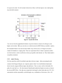
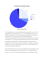
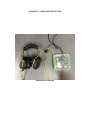
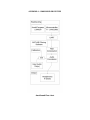
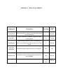
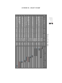
OmniSound
Submitted To
Gustavo de Veciana
Kevin Connor
Cisco
Prepared By
Dalton Altstaetter
Marc Hernandez
Rounok Joardar
Jeffrey Mao
Brian Russell
Jason Weaver
EE464 Senior Design Project
Electrical and Computer Engineering Department
University of Texas at Austin
Fall 2014
CONTENTS
FIGURES ..................................................................................................................................... iv
EXECUTIVE SUMMARY ........................................................................................................ 1
1.0
INTRODUCTION........................................................................................................... 2
2.0
DESIGN PROBLEM STATEMENT ............................................................................ 2
3.0
4.0
2.1
Problem Definition .............................................................................................. 2
2.2
Specifications ....................................................................................................... 3
DESIGN PROBLEM SOLUTION ................................................................................ 4
3.1
Underlying Theories and Operating Principles ............................................... 4
3.2
Key Decisions ....................................................................................................... 4
DESIGN IMPLIMENTATION .................................................................................... 7
4.1
5.0
LSM9DS0 Sensor ................................................................................................ 7
4.1.1
Configuration ........................................................................................... 8
4.1.2
Calibration................................................................................................ 9
4.1.3
Orientation Calculations.......................................................................... 9
4.2
Integrating Headtracking................................................................................... 10
4.3
Audio Convolution .............................................................................................. 11
4.3.1
GUI ........................................................................................................... 12
4.3.2
Dynamic Filtering .................................................................................... 12
4.4
Latency ................................................................................................................. 13
4.5
Open House Demo............................................................................................... 14
TEST AND EVALUATION .......................................................................................... 14
5.1
Component Testing ............................................................................................. 14
5.2
Subsystems Testing ............................................................................................. 15
5.3
5.2.1
Headtracking ............................................................................................ 15
5.2.2
Audio Filtering ......................................................................................... 17
5.2.3
Subystem Integration ............................................................................... 18
Prototype .............................................................................................................. 18
CONTENTS (Continued)
6.0
7.0
8.0
9.0
TIME AND COST CONSIDERATIONS .................................................................... 21
6.1
Headtracking Delays ........................................................................................... 21
6.2
Headphone Delays............................................................................................... 22
SAFETY AND ETHICAL ASPECTS OF DESIGN ................................................... 22
7.1
Safety Factors ...................................................................................................... 22
7.2
Ethical Issues ....................................................................................................... 23
7.3
Public Interest ..................................................................................................... 23
RECOMMENDATION ................................................................................................. 24
8.1
Alternative Computational Methods................................................................. 24
8.2
Implementing the Gyroscope ............................................................................. 25
8.3
Optimizing Gain .................................................................................................. 25
CONCLUSION ............................................................................................................... 26
REFERENCES ........................................................................................................................... 27
APPENDIX A – OMNISOUND PORTOTYPE ................................................................... A-1
APPENDIX B – USER MANUAL ......................................................................................... B-1
APPENDIX C – BILL OF MATERIALS .............................................................................. C-1
APPENDIX D – GHANTT CHART ...................................................................................... D-1
FIGURES
1. System Accuracy ..................................................................................................................... 16
2. System Deviation ..................................................................................................................... 17
3. System Latency ........................................................................................................................ 19
EXECUTIVE SUMMARY
This document discusses Omnisound’s problem statement, design problem solution, design
implementation, our testing and evaluation, time and cost considerations, safety and ethical
aspects of our design, and our recommendations to improve upon Omnisound.
In the design problem statement our team explains how Omnisound will address and assess
issues in current binaural audio with headtracking implementations. The biggest issue our team
assessed was latency. Creating a system with low latency, high accuracy, low cost, and high
portability is highly sought after in the 3D audio field. After researching human auditory
perception, our team found that latency exceeding 60 ms, or accuracy exceeding 8.3 degrees,
would break the illusion of a 3D audio scene adjusting accordingly to head movement.
Omnisound succeeded in its accuracy but exceeded in its latency by 20ms, perceptible to some
users. Also in order to create the illusion of 3D audio, Omnisound needed to rotate sound 360
degrees around the users head, which it did successfully.
The design solution and the design implementation sections in our report discuss the underlying
principles and decisions of creating 3D audio with headtracking. Furthermore, these sections
discuss the hardware and software components needed to create 3D audio. The implementation
to create 3D audio is to take the head position, use this position to index to a pre recorded Head
Related Transfer Functions, HRTFs, and mixes them with an audio source. HRTFs are sounds
recorded at multiple positions 1 meter around a Kevlar dummy’s head to simulate how the ear
hears sound at different points around the head. To realize our implementation, we used
MATLAB to get head position data from our headtracking sensors, index though a library of
HRTFs that correspond to the head position, and do real time audio processing that produces
audio to the headphones.
To ensure that Omnisound addressed our problem statement this document also includes our
tests and evaluations that explain our accuracy and latency test results. While our team was
testing Omnisound we ensured that our project was in compliance with safety regulations and
confirmed that we followed the IEEE Code of Ethics to provide a solution that is beneficial to
the publics interest.
Upon completing OmniSound our team has recommended alternative implementations to
improve our design. The first recommendation would be to use software that can handle real time
signal processing, for OmniSound this means not using MATLAB to decrease computational
overhead. The second recommendation would be to add a gyroscope in our existing design, this
will increase accuracy in headtracking. Finally, our team recommends optimizing the
frontal/back gain around the head to create a more immersive 3D audio.
1.0
INTRODUCTION
This document describes our team’s efforts in designing OmniSound over the course of the last
two semesters. OmniSound is a 3D audio system that incorporates headtracking to generate a
highly immersive soundscape. This audio system provides the illusion of natural sounding audio
by using 3D audio filtering to add a sense of directionality to the sound and using headtracking
to aim that sound at the user.
Previous reports have discussed the development of OmniSound in parts. In this report we will
cover the full story of OmniSound from start to end, thereby giving any reader a complete
understanding of the development of this project. We will begin by describing our initial goals
and the requirements and specifications we wanted OmniSound to meet. Then we will discuss
the plans and ideas we conceived in order to meet our goals. This will be followed by a detailed,
technical look into what we actions we took to make our plans a reality culminating in the final
prototype of OmniSound. This section will contain the majority of the work we did in designing
our final prototype. We will go over the budget we used and the safety in using OmniSound.
Finally we will close with our thoughts on the future of OmniSound.
2.0
DESIGN PROBLEM STATEMENT
Before attempting to create a design solution, we needed to have a thorough understanding of our
design problem. Additionally, it was important to lay out the goals and specifications we needed
OmniSound to meet. Knowing our target parameters and major obstacles, found through
research, was crucial to creating a solution that would satisfy the client’s project needs.
2.1
Problem Definition
OmniSound aims to improve the quality of stereophonic audio. Stereophonic sound, or stereo, is
used to mimic a 3D sound environment. It achieves this by outputting two or more audio
channels through different sound filters in order to create an illusion of directionality. When a
person moves his head, he changes the direction in which he perceives sound. Current systems
have no way to accommodate for this change in positions. Our purpose will be to design a
system that can sense a user’s head movement and adjust the audio filters to preserve a more
realistic sound environment.
This system would greatly improve the audio quality of headphones for a low cost. It would
allow for greater distinction between sounds and create a more natural imitation of the
soundscape. While the system would be applicable to a number of different scenarios, this
project would be most applicable to users in long distance conferences by enhancing the quality
of their telecommunications. Other uses might include faster than sound flight, where sounds
must be simulated in order to make them audible to pilots. 3D audio also has a place in creating
new virtual realities. In any case, creating effective binaural audio gives us innovative new ways
to interact with the world around us.
2.2
Specifications
Before beginning construction it was important that we identify the parameters and specifications
we would need to work around. Though the overall sense of immersion will be subjective there
are a number of items that we can standardize to improve the quality of the product across the
board.
Our primary constraint is latency. Latency is the time between a user’s head movement and the
audio output. We found that OmniSound should have a latency of no more than 60ms [4].
Exceeding this bound is highly likely to cause the illusion of 3D audio to dissolve. As a result,
this is the utmost priority during construction of OmniSound.
We also understood that maintaining a reasonable degree of accuracy would be another key
factor. But to discover the exact specifications a very basic idea of how OmniSound would be
built was needed. We decided that there would utilize two main components. A system of
headtracking and a system of 3D audio generation software.
The headtracking system has to be accurate to within 8.3° of the actual angle [2], the minimum
angle, indicated by our prior art research, that humans can differentiate different audio positions.
Also, to ensure headtracking is minimally intrusive to the user, the headtracking unit cannot
weigh more than 20g. The headtracking system must also operate at a voltage of 3.3V, the
voltage obtainable from a standard USB port or external batteries [1]. To be easily placed atop a
pair of headphones, the sensor board placed on the user’s head must not exceed 1.1" x 1.6" (28 x
41mm) [1].
The 3D audio waveform generation software requires at least a 50 MHz clock speed, which is
equitable to existing video communication software [3]. OmniSound must also pass several
performance benchmarks. The system response from input to output cannot take more than 60
milliseconds (ms) [4], otherwise, the illusion of 3D audio breaks down. Spatially, OmniSound
must simulate an audio source in a specified radius around the user’s head.
3.0
DESIGN PROBLEM SOLUTION
Our design solution is composed of a description of the underlying theories that led us to this
solution, a summary of the root principles and that form the base functionality of OmniSound,
and an outline of how we implemented the solution we came up with, as well as key decisions
that shaped the development of OmniSound.
3.1
Underlying Theories and Operating Principles
Any solution to our design problem needs to truly simulate 3D sound. That is, it needs to
preserve the illusion that sounds are coming from distinct locations around the user, not relative
positions that move along with their head. The only way to achieve this illusion without using
fixed speakers for each sound source is to modulate each source so that sounds as if it is coming
from a fixed position. Since the human brain recognizes the direction a sound is coming from
based on how the sound is affected by the shape of the ear, it is possible to simulate sound from
an arbitrary point by mimicking the ears’ effects through audio convolution.In order to simulate
a fixed point using headphones that rotate with a person’s head, it is necessary to counter this
motion by simulating movement of the audio source in the opposite direction by changing the
filter the audio is convolved through.
3.2
Key Decisions
To accomplish this dynamic audio convolution, or modulation, OmniSound uses a library of
HRTFs. The library we used was created by recording the response that microphones in a model
of the human head have to sounds at many different angles of azimuth and elevation around the
model, and then using an inverse function to determine what filter would have the same effect on
an audio sample. Each HRTF maps to a specific point in space around the user. Changing the
HRTF changes the perceived sound location. Omnisound works by choosing one of the filters in
the HRTF library based on the position of the user’s head and passing a short snippet of the
output audio file through the filter.
Once a solution is able to simulate an audio source at any location, it needs to be able to
determine which location to put each source in real time, so a head mounted solution to our
problem would need to be able to somehow track a user’s head movement. In the end, we
decided to use a combination of an accelerometer, which can measure changes in angular
position relative to gravity, and a magnetometer, which functions similar to a magnetometer by
measuring changes in angular position relative to the Earth’s magnetic field. These two sensors
combined allow us to track the user’s head along two axes of rotation, which is sufficient to
determine an absolute angular position. We considered other options for how our solution would
track a user’s head, however. We ultimately decided to use the accelerometer and magnetometer
for a few key reasons: neither the accelerometer nor the magnetometer suffer from significant
drift in measurement over time like our other considerations, such as a gyroscope. Also, the two
sensors are most accurate along different axes, so we are able to accurately cover more angular
positions.
Early on, we had to make a decision as to whether we would be using a set of sensors mounted
on the user’s head (active headtracking) or a software based camera input analysis (passive
headtracking). We chose not to use passive headtracking because it would require more
complicated software and increase the latency between when the user moved their head and
when the system received a measurement. We decided to use active headtracking for these
reasons. To implement an active sensor based headtracking system, we needed to make a few
key design decisions: what sensor should we use? How would we interface with the sensor?
What kind of microcontroller would we need to have as an intermediary between the sensor and
computer? What computations if any would need to be done on the microcontroller? These
questions have shaped our progress over course of the year.
Our two main choices for headtracking sensor were the Razor IMU and the LSM9DSO. The
Razor sensor has a built in microcontroller, is only compatible with the I2C communication
protocol, and was much more expensive than the LSM8DSO, which is slightly smaller, requires
a microcontroller to interface with a computer, and is compatible with both SPI and I2C. So that
we could keep our options with regard to the serial protocol we would use open and because it
was the cheaper part considering that we already had a microcontroller, we decided to go with
the LSM9DOF sensor. To interface with the sensor, we considered using SPI and I2C. The SPI
protocol uses more lines than I2C, because each line can only either send or receive data, not
both. Because of the simplicity of transfer along each line, SPI is also faster. On the other hand
I2C uses fewer lines that can both send and receive data. I2C is slightly slower and more error
prone than SPI. These reasons contributed to our decision to use SPI to communicate between
our microcontroller and our sensor. As previously stated we already had a microcontroller, which
factored into our decision to use the LSM9DSO, and we had no reason to use a different
microcontroller since it would only function as an intermediary between our sensor and the
computer, so we decided to use our TI LM3S1968. Since we would have a microcontroller
between our sensor and computer, we had the opportunity to perform some calculations on the
sensor data before it was sent to the computer. We decided to use this opportunity to speed up
our calibration process by performing calibration and correcting measurements on our
microcontroller. In the process of answering these questions, we developed our plan for
implementing the hardware headtracking portion of our design.
Once the computer receives the angular measurement from the headtracking module, we needed
to use this angle to update the position of the simulated audio source. To make this adjustment,
we must read the sensor input from the COM port, and select which HRTF would be the best fit
for the angle received. All of these operations could be relatively simply implemented using
almost any programming language as a base. The exception is reading the COM port. Most
programming languages that our team had experience with have convoluted processes for
reading device input, so we decided to use a MATLAB script for the software portion of
OmniSound. MATLAB has many built in interfaces for device input as well as audio output,
both of which would take additional time designing in most other languages. These benefits, as
well as the familiarity our team had with MATLAB led us to choose matlab as our programming
platform. This decision was a significant factor in our inability to meet our latency requirements
however. The overhead that MATLAB adds to both reading the sensor input and outputting the
resultant sound was more than 80% of our final latency. In order to determine which filter would
be used at any time in our software we needed to either load in from a file the filter that
corresponds to the user's head position or select the appropriate HRTF from a collection of preloaded filters. We decided to load the entire HRTF library into memory at the start of the
program to reduce the time spent every time the HRTF is changed at the cost of additional start
up time and increased memory usage.
In retrospect, our design solution was subjectively successful, with most users reporting a
positive experience. However, we didn’t quite meet some of our key product specifications. Our
research found that the human ear is unable to detect up to a 60 millisecond latency between the
expected sound and when the actual sound occurs. Our solution was only able to reduce our
latency to 80 milliseconds. The area in which an alternative solution could have improved this
latency the most was in our decision to use MATLAB as the basis for our software portion. Since
such a large portion of our latency was caused by MATLAB overhead and the need to reduce the
input sample rate in order to achieve an acceptable sound quality. If we had implemented our
software module in a lower level programming language we could have significantly reduced our
latency at the cost of increased development time.
4.0
DESING IMPLEMENTATION
Overall, our design closely followed our Gantt Chart from last semester with some exceptions,
see Appendix D. There were several unanticipated design changes that needed to be made
during the semester. These changes mainly occurred in the headtracking module. Despite these
setbacks, we were able to make up lost time without impacting our projected finish date.
4.1
LSM9DS0 Sensor
We made several modifications from our original design and our final implementation. In our
subsystem testing, we encountered problems interfacing the LSM9DSO with the LM3S1968
microcontroller using the Serial Peripheral Interface (SPI) protocol. We were not able to debug it
directly since it is a clocked protocol and any debugging that interferes with the timing of the
protocol will inherently cause errors during data transfer. To fix this problem, we used a digital
logic analyzer as our main debugging instrument to view the signals changing so we do not
affect the timing. After viewing the timing diagram on the digital logic analyzer, we caught
errors in the initialization of the SPI protocol within the microcontroller and changed the clock
polarity (CPOL) and clock phase (CPHA) which determine whether the data is latched or read on
the rising or falling edge of the clock. This allowed interfacing with the LSM9DSO and
we verified communication with the devices by viewing read-only registers with fixed quantities
and checked to see that it matched the datasheet specifications.
4.1.1 Configuration
Once we were able to communicate with the LSM9DSO the next step was to program it. We
initially were going to use the gyroscope and accelerometer for the headtracking. We initialized
the LSM9DSO to sample the three gyroscope orientations at an output data rate of 760 Hz and
with a cutoff frequency of Fc = 100 Hz [5]. This gives us the most accurate gyroscope
information and sets our lower bound of our latency limit at 1/Fc = 10 milliseconds since if we
are any faster we will run into the problem of aliasing. The gyroscope range was chosen as + 500
degrees per second (dps), this would be more than enough to detect fast head movements with
the best precision since people cannot turn their head even 360 degrees [5]. The next lowest
range was + 245 dps which could be insufficient for fast head movements across the full range of
head motion [5]. The accelerometer output data rate was sampled at 100 Hz since it has a low
frequency response and sampling at higher rates does not add any value and consumes more
power.
After configuring our settings for the accelerometer and gyroscope we soon found out the
difficulty in using a gyroscope because we lacked the ability to verify its accuracy. The 16-bit
signed gyroscope measurements have units of change in ADC sample/second ranging from 32768 to 32767. However, since the gyroscope measurements are a function of time, in order to
check its values we have to know at what rate the gyroscope is being moved angularly. We did
not have an instrument available that rotated at a known radians/second. This presented a
significant problem since we chose to use the active sensor and knew that this was possible but
were not aware of the additional equipment needed to test it. This was a time consuming setback
and required researching other method to determine the elevation and azimuth of the head
position. We found a method that used the magnetometer and the accelerometer. Using two
absolute coordinate systems also seemed an advantage to using one relative coordinate system
and one absolute in terms of reliability testing. The drawback was that magnetometer readings
vary depending on the interference that comes from other electronic devices. We used vector
calculus equations to re-orient the axes and were able to calculate elevation and azimuth [6].
4.1.2 Calibration
Now that we could get the azimuth and elevation the next step was to calibrate our readings from
the LSM9DSO to remove the DC offset. This had to be done for each axis of the accelerometer
and magnetometer and is done by taking summing the maximum and the minimum values and
dividing by two and adding that to that corresponding axis. We had several problems with our
automatic calibration in which we rotated the LSM9DSO around and stored the maximum and
minimum values for each axis. this was because of outliers in the sensor readings that can be
attributed to noise and time before the sensor settles after being initialized. Our solution to this
was to enter the calibration by hand so that those outliers did not skew our reading. This was a
time consuming and tedious process prone to human error since it requires someone to observe
what the average maximum and minimum values seem to be. This also was inadequate and we
went back and modified our original automatic calibration and restricted it to find the maximum
and minimum only along fixed axes rather than trying to find them along any orientation. This
was much less error prone and helped avoid the previous problem by avoiding outliers since it
was moved along a fixed axis which more closely resembles the motion of someone’s head
movement and is ideal for system performance on a fixed vertical elevation.
4.1.3 Oreintation Calculations
In our initial design we were going to do the calculations for the elevation and azimuth within
the microcontroller. Upon implementation on our fixed-point processor, we were using
optimized fixed-point operations for square root using Newton’s method, atan2, atan, sine, and
cosine. However, we soon ran into problems relating to overflow, correct scaling of data before
calculations, and rounding resulting from truncation. Our initial reasoning was that using fixedpoint operations would drastically reduce latency over a floating-point representation. On the
contrary, there were many bugs associated causing the microcontroller to become stuck in
infinite loops due to overflow and underflow. If we were conservative on our estimates then we
would not be using our full range of 32-bit values effectively and would lose a significant
amount of precision. On the other hand, the greater range of values we used the greater chance of
overflow. This was complicated by the doing multiplication of 16-bit numbers which already
maxes out our full 32-bit range and guarantees loss of precision. As the number of calculations
compound, more precision is lost along the way. Our initial idea was to send the elevation and
azimuth to MATLAB to be processed. We soon found this to be a task unsuited to a general
purpose microcontroller limited to a fixed-point processor. We reasoned that since there would
need to be communication with MATLAB that we would do all the processing in MATLAB
using double-precision. We concluded that we would have more computation power using a PC
for the calculations that the trade-off between fixed-point and floating-point would be nominal at
least and, potentially, performance enhancing at best. At that point we determined to use the
microcontroller as a debugging and polling instrument to gather accelerometer and
magnetometer data and send the raw data directly to MATLAB.
4.2
Integrating Headtracking
Integrating the headtracking data with the MATLAB filtering module came with its own issues
with data transfer. We used the Universal Asynchronous Receive Transmit (UART) which sent
bits, clocked serially, at baud rate 9600 bits per second. This baud rate was initially much higher
in testing but was modified after making the final prototype. A higher baud rate reduces latency
but the signal degraded severely in our 10 ft ribbon cable. The microcontroller is constantly
sampling the LSM9DSO and always has the most recent headtracking data. In our initial
implementation we were constantly sending the headtracking through the UART even if we were
not reading the data into MATLAB. We thought this would speed up a transmission since all that
was necessary was to open the receiving side of the UART in MATLAB. However, we quickly
discovered what we thought were incomplete data transmissions. We learned that when we
opened the UART port in MATLAB, our first byte we would get would arrive somewhere in the
middle of a data transmission. To fix this problem, we no longer would continuously transmit
data from the microcontroller, but would instead only transmit the data on request. Before each
read, the microcontroller would poll the UART to see if a UART transmission was requested. If
a transmission is requested, it would transmit the current data and then assume the normal
execution path of reading the headtracking data. Although this increased the latency, this allowed
us to guarantee the order in which we receive the data without having to modify the transmission
to tell different data transmissions apart from one another.
4.3
Audio Convolution
The filtering subsystem convolved the input audio with the Head Related Transfer Function
(HRTF) to create binaural (directional) audio. We first started with binaural audio in a static
environment where the direction of the audio was pre-determined by us in our MATLAB script.
Our first goal, was to test the extremes filtering with the HRTF coefficients for +90 and -90
degrees. This proved successful, and we soon sought to change the source position rather than
having a fixed direction for the sound clip. We created a sound file in which we had the source
move a full 360 degrees around the user’s head in 15 degree movements. However, we noticed
the audio quality decreased during the process and heard intermittent “popping” indicating when
we switched HRTF filters. We discovered a couple reasons for this. We hypothesized that the
using HRTF filters with a precision of 15 degrees was too large. We found there were other
HRTF filters that had precision of 5 degrees and used these in place of the original filters. There
was no discernable difference when comparing the audio when using the higher resolution HRTF
filters. This led us to believe the problem was related to using the MATLAB function convolve
which spreads the spectrum of the audio to n+m-1 where n is the number of audio samples being
convolved and m is the number of HRTF filter coefficients used in the FIR filter. Increasing the
number of samples changes the frequency of the audio due to the group delay of the filter. By
doing this on each audio frame being filtered we were modifying the audio and reducing the
quality. To resolve this, we used MATLAB’s filter function, which returns the same number of
output samples as there are in the input samples. This greatly reduced the level of popping but
did not get rid of it completely. It was not until we consulted Dr. Brian Evans that we realized we
should have been saving the output filter coefficients from each filtering operation to use as
inputs for the next HRTF filter. This solution eliminated all audible “popping.” Now, we had a
stand-alone prototype simulation for an ideal case when there is no latency associated with
acquiring the headtracking position. We would use this as a template for the dynamic filtering.
4.3.1 GUI
Before we can implement our dynamic filtering we first had to build a simple interface with
which a user could interact with our software. To achieve this we made a Graphical User
Interface (GUI). The goal of the GUI is to initialize the processes required to run our system. The
GUI accomplishes two main tasks: 1) taking the path to the HRTF filter library and reading the
filter coefficients into MATLAB. 2) Selecting the audio file the user want to use as the audio
input. We give the user some freedom in steps 1) and 2) therefore stringent error testing was
done to assure that the user selected the correct folders for the HRTF library and that the user,
did in fact, select a valid audio file. If these assumptions were not met the project would wait
until it has the valid HRTF libraries and an audio file. Once it has these two valid inputs, It
would call the dynamic filtering script which would run the system.
4.3.2 Dynamic Filtering
In building the dynamic filtering we realized MATLAB’s deficiencies in implementing a realtime audio system. The tools that worked well for our original static simulation were not
available in the dynamic system. The dynamic filtering required changing three main parameters
associated with playing the audio through the computer’s sound card. Of these three parameters
there is only one independent parameter, with the other two being dependent on other variables.
The first (independent) parameter was the time per frame. Filtering the audio dynamically
requires break the input audio file into frames. The number of samples in a frame is dependent
on the time per frame. Since our sample rate is CD quality of 44.1 kHz the number of samples
can be calculated by (44100 samples/second) * (X seconds/frame) = 44100 * X samples/frame.
The next (dependent) parameter is the sample rate and is fixed based on the audio. As previously
noted, our sample rate was 44.1 kHz. The final (dependent) parameter is the number of samples
per frame, which was calculated above as 44100 * X, where X is defined as the number
seconds/frame. To understand how to optimize our one independent parameter it required
understanding how MATLAB interfaced with the computer’s sound card on a hardware level.
The MATLAB documentation used a queue to store the audio samples. The time per frame
determined the size of the queue [Matlab documentation backing this up]. If we failed to allocate
a large enough queue we ran into underrun problems and our output audio wouldn’t play from
the sound card. If we allocated too many samples the latency performance was unacceptable and
did not meet our 60 ms latency upper bound. This required a significant amount of time to find
the optimal trade-off between low latency audio and audio quality. One way we reduced the
latency was to truncate the HRTF filters from 512 coefficients to 256 coefficients. This would
speed up our on-going calculations being computed while the last frame was playing through the
sound card. Our latency requires the time per frame to always be less than the filter computation
time. this is because these operations are being done in parallel and if our sound card is finished
playing the audio before we have put the next frame into the queue, then we get the queue
underrun warning since MATLAB is attempting to play audio that has not yet been sent to the
queue and the sound card outputs noise until the next frame is loaded into the queue within the
time specified in time per frame, which may carry over for several seconds of audio, not just the
next frame. This details the importance of correctly selecting the time per frame since it has a
ripple effect that may last for up to several hundred frames and seconds of audio.
4.4
Latency
The bottleneck of the latency occurred in the first transmission of the queue to the sound card.
This characterized the lower bound for all other transmissions and determined how far behind in
time our most recent headtracking coordinates were. The calculation time for filtering was on the
order of tens of milliseconds and the queue latency was in the range of 30 to 50 ms to transfer the
audio to the sound card. One solution we found to reduce latency, on a hardware level was use
sound card drivers that interface directly with the sound card hardware, bypassing the windows
drivers. These drivers were called ASIO4ALL. There was potential for these drivers to work too
well, in which the latency was so low that we would not be able to finish the filter computations
before a new frame was being output to the sound card and another queue underrun would occur.
When testing the ASIO4ALL drivers we immediately got the queue underrun warning and heard
the “popping” associated with underrun. This was expected and verified the latency reduction
when bypassing the windows sound card drivers. This had the effect of reducing latency after
exhausting other methods of optimization through software.
4.5
Open House Demo
Our final task was to determine how to best demonstrate our working prototype at Open House.
This was something we had thought about months in advance of Open House since it could
change the design depending on the features we chose to focus our demo on. One idea was to
place several directional audio sources in space with the sound sources being at fixed angles
relative to the each other but with the user’s head being relative to all the sources. Implications of
this include moving the sound sources around the user’s head but keeping the sound sources all
coming in at a different direction as perceived by the user. This is the embodiment of our project
since this would all be done in real-time and would accurately simulate what someone would
hear in a normal soundscape with authentic sounds as opposed to our simulated audio. This idea
seemed promising since it exemplified the design problem our project intended to solve. To our
dismay, when we tested it, the audio was overwhelming to the extent that it was detrimental to
the illusion of binaural audio and did not naturally replicate what a person would hear in a
soundscape. In effect, we simplified our dynamic demo to play a single directional sound to
demonstrate the effectiveness of our design without overwhelming the user. In conjunction with
our dynamic filtering demo, we had our static demo available for people to listen to. This was
our initial simulation that played an audio file from 0 to 360 degrees and showed how the
concept was effective in an ideal situation. The goal of our demo was to educate people about
binaural audio and based on the responses at open house the feedback was overwhelmingly
positive.
5.0
TEST AND EVALUATION
To verify Omnisound we tested it at the component, subsystem, and prototype level. Overall,
our testing focuses on the latency, accuracy, and the listener's perception of the system. For
more background information on our testing plan, refer back to our previous Testing and
Evaluation Plan.
5.1
Component Testing
When we began constructing our head tracking system, we tested the individual components as
we received them to avoid possible defects later in the process when they could be more costly.
Omnisound utilizes three different components: the sensor (LSM9D0 breakout board), the
microcontroller (LM3S1968), and a pair of over-ear headphones.
We first confirmed the sensor and microcontroller were working. We conducted two yes/no tests
that checked whether we could download code into the microcontroller and whether the UART
could send/receive data. Both tests were successful. We then tested that the sensor generally
measured the magnetometer’s north heading and the accelerometer’s gravity heading. It is
impossible to unmarry our interpretation and calibration of the sensors data from the sensors
themselves. Thus at the component level, it is sufficient to know that they pointing in a
direction.
Our headphone tests were also successful. We qualitatively decided that the headphones had a
standard balance and sufficient noise isolating for open house. No malfunctions arose, but we
had duplicates of all physical components for any unforeseen circumstances. Having run these
tests, we are confident that all physical components are functioning properly.
5.2
Subsystems Testing
Omnisound has 2 subsystems (shown in Figure 1): headtracking and audio filtering. Both
systems are closely integrated, so we tested both that the two major subsystems worked
individually and successfully with each other.
5.2.1 Headtracking
First we measured the accuracy of our computed angles from the actual angles. To do so, we
followed the following procedure. First, we labeled a polar grid like the one shown below. Next,
we laid the polar grid parallel to ground. Third, we moved the sensor to point at label 1 330
degree. Fourth, we looked azimuth read by the sensor. We then recorded this data on a graph,
and repeated the process 12 more times for test points 1 through 12.
Figure 1. System Accuracy
Based on Experimental results, our head tracking system is reasonably accurate. However, the
error of our headtracking unit seems to increase the further we go away from the original point of
measure. This is because the headtracking unit reorients everything based on an initial starting
vector front. The further one goes away from front the larger the error becomes hence why 5 and
6 which are the back of the head have the worst accuracy. This is within our accuracy limit;
because, the human head can only turn itself 90 degrees right or 90 degrees left meaning only
test points: 9,10,11,12,1,2, and 3 are really going to be useful.
We then measured how much Omnisound deviates from a value by collecting values when our
prototype was stationary. The average deviation of the elevation was 1.528 degrees. As our
HRTF library is incremented every 10 degrees in the elevation direction, that standard deviation
is well within acceptable limits. We then leave the sensor on in the same position for 15 minutes
to see the drift of values along init. As long as our drift is under 8.3 degrees, we will accept our
values as consistent. Now consider the deviation of the azimuth shown in Figure 2. The Purple
Line represents our experimental deviation of azimuthal values for different Elevations. The
yellow line represents the accuracy at which the error becomes perceptible to the human ear, 8.3
degrees [2]. The Red Line represents our ideal standard deviation, half of the azimuthal precision
for a given elevation. For all variance below the red line, it will not improve our sound quality
any noticeable amount.
Figure 2. System Deviation
You can see from the graph that the further away the elevation is from level (0 degrees), the
higher our deviation. What you can also see is that because the HRTF library resembles a sphere,
the azimuthal distance also increases the further away from level (ex: 90 degrees elevation
rounds all azimuths to a single point). Thus our experimental line is almost completely within
our ideal variance, and it is well below what is perceptible to the human ear. Thus Omnisound is
acceptably consistent.
5.2.2 Audio Filtering
We first tested the audio file and head angle that is the user input. After presenting the midsemester Oral Progress Report, our corporate sponsor from Cisco clarified that Omnisound
doesn’t need to support different inputs and platforms. Thus we only verified valid audio file
paths for .mp3 and .wav. We then ensured OmniSound rounds head angles correctly to chooses
the closest HRTF filter. Note that users input their head angle by their head and not a GUI. We
automated a test that sequentially cycled through every combination of elevation (-40 to +90
degrees) and azimuth (0 to 360 degrees). It confirmed that a file was found for every
combination, and it ensured that the difference between each input and result was no more than
ceiling(input) / 2, choosing the closest HRTF.
Even though we were then sure Omnisound was rounding to the nearest HRTF correctly, we
conducted preliminary tests by typing an angle into a GUI and having the user guess the
location. We had a perfect general localization except when the HRTF was directly in front or
behind the user. The result was not surprising as it is a flaw of the human ear.
5.2.3 Subystem Integration
We then tested that the UART was correctly transmitting data. The test continually sent a stream
of consecutive numbers from the microcontroller. Then computer input a set of consecutive
numbers and checked to see if MATLAB head read the same set. The success of the test ensures
that the UART correctly transmitted the data without introducing any error or losing data. We
also tested latency of this component and the microcontroller at a baud rate of 9600 bits per
second. Everything from reading the sensor to sending the data to MATLAB takes no more than
2 ms.
5.3
Prototype
Once the prototype was complete, we began testing the latency of the full system. This was done
using MATLAB’s internal time profiling functions and users’ judgement. We recorded the
latency of 25 audio steps at the component level. Figure 3 represents these latencies after we
took the rounded ceiling after throwing out the outliers.
Figure 3. System Latency
The two biggest latencies are retrieving the angle from the microcontroller (18ms = 22.5%) and
outputting the audio to the computer (46 ms = 57.5%). Even though the microcontroller can
transmit everything in under 2 ms, the MATLAB input/output overhead increases the latency to
an irreducible 18 ms. The output deals with the same MATLAB input/output
overhead. MATLAB pushes the audio section to a buffer, and the computer comes and pushes it
to the headphones. Even with decreasing the buffer and accurately syncing when the computer
wipes the buffer with when the buffer is written to (both functions of the size of the audio
sample) the component latency was over half of the whole latency. Originally we estimated that
the filtering (5 ms = 6.25%) would be a big factor, and we had ways of truncating the process,
but they proved insignificant comparatively.
We previously defined success to be if on average the difference between requesting the raw data
from the sensor and outputting the audio out is less than 60ms. The components of Figure 3
equate to 71 ms. What’s more, is that when audibly tested by users, we found 80 ms to be the
minimum acceptable latency. Why? Real-time processing is simply being able to compute and
output a sample in less time than the sample takes to play. When the sample takes less time than
everything else, small gaps or pops happen in the audio. We attribute the extra 9 ms (actual
latency - measure latency) to outliers that sometimes take longer than measured and the time the
audio takes to be read from the buffer and output into the user’s headphones.
Omnisound also met the required specifications that didn’t need tests. First it met the weight
requirement. The sensor only weighs 2.3g and even with the ribbon wire it is far below the 20g
limit. The small board is also within the size specification and fit neatly on the headphone
band. Also, all of the hardware was run off of a single USB port. Lastly our system did replicate
a sound environment at a radius around the user’s head, but not with complete success. Many
users claimed that the sounds sounded very close to the instead of at a 1m distance. We believe
this to be a limitation of the HRTF library that we chose.
Lastly, we tested Omnisound with some members of other groups in our Senior Design lab and
presented it at the open house with this accuracy, deviation, and latency. We previously put
numbers and percentages on how we would deem accuracy sufficient, but they did not work in
practice. Pointing was much more practical to identify a spherical direction, and all users were
able to locate the position of the “stationary” sound. Again, we experienced some confusion
directly in front and behind the user, but it was expected. In this we said the accuracy and
deviation were sufficient. Next, we already knew Omnisound was 20 ms longer than our
research said was perceptible, but we wanted to know if it was perceptible in our tests. No one
on our team could detect the delay unless we thrashed out heads back and forth, and only two
people at the entire open house mentioned hearing a delay. Note that it is probable that more
people heard the delay, but did not voice it. In this we said that we did fall short of the latency
requirement, but it would not be that detrimental or noticeable in regular use such as in a
conference call. Overall it is important to note that most users reported a positive user
experience.
6.0
TIME AND COSTS CONSIDEATIONS
We successfully met our time and budget constraints. Although there were some implementation
setbacks, Omnisound was completed within our time constraint. Budget was never an issue for
OmniSound; because, our implementation is cheap easily under $300, see. The two main
setbacks we faced were implementing our headtracking module and our headphones arriving
later than expected.
6.1
Headtracking Delay
When implementing our headtracking module we found that the accelerometer and the
gyroscope pair was insufficient for calculating azimuth. The accelerometer can not help
compensate for the natural drift of the gyroscope along the XY plane; because, the accelerometer
only naturally senses gravity which points down in the Z vector. Without an X or Y reference
vector, the gyroscope will uncontrollably drift way off target for in intervals of time as short as
one second. As a result, we moved toward the magnetometers, which has an XY reference
vector, magnetic north. Marc, Jeffrey, and Dalton focused on implementing the new
headtracking design while the rest of the team remained focused on convoluting the HRTF
functions in MATLAB. This delayed our headtracking completion by half a week. The
LSM9DS0 included a magnetometer attached, so we did not need to order new parts. This
allowed our team to reuse most of the old gyroscope code in the new configuration. Once we
implemented the magnetometer , we realized that the measurements lose a lot of accuracy when
the head tilts up and down. Marc and Jeffrey then had to research methods to compensate for the
tilt. Jeffrey came up with a solution in three days. We used the accelerometer to calculate the
users position in the up and down direction and used that angle to compensate reorient the
magnetometer’s azimuth. This solution did not have the drift of the old solution, and could
handle the tilt fairly well within a reasonable range. Because our accelerometer was already
implemented, we were able to successfully implement the formula’s within one day. All
together, we were able to minimize the time lost from researching and implementing the solution
to one week. However this change ran us into another problem, the electronic magnetometer
needs calibration. We had to spend another week developing automated calibration software to
smooth the set up process. Altogether, our schedule was pushed back two weeks from our
planned schedule, we compensated for the lost time by cutting our user testing period short.
Thankfully, the use case studies, we did do were mostly positive, and we feel that we did not lose
too much data from cutting our testing time.
6.2
Headphone Delay
We ordered the headphones earlier than we needed to in case the the order should take take
longer than expected. However, our headphones managed to take longer than we thought it
would. In fact, they arrived in the middle of November. Our team was able to get around this
delay by testing the headtracking module on our personal headphones. This allowed us to
complete most of the testing before our ordered headphones arrived. Afterwards, we constructed
the fully working prototype and test it in one day. As a result, we were not delayed and
completed our headtracking module on schedule.
7.0
SAFETY AND ETHICAL ASPECTS OF DESIGN
Omnisound adheres to safety and ethical standards that protect the the public's interests. The
safety and ethical standards are set to protect the user from injury and the environment by
properly disposing the electrical components used in Omnisound, if need be.
7.1
Safety Factors
During Omnisounds implementation, many safety factors were considered in order to protect the
user from being injured. Omnisound is constructed with over the ear headphones, a
microcontroller, and a headtracking sensor. The headphones consist of a cable, two speakers, a
headband, and ear pads. The the wires within the cable are covered by insulation that protects the
user from being shocked when the earphones are plugged into the computer. The volume at
which the speakers produce sound is controlled by the user. The Occupational Safety and Health
Administration,OSHA, recommends to the general public to keep volume levels below 85decibels, this is equivalent to a running lawnmower [7]. The headband, that presses the speakers
against the users ears, are built to fit various head sizes. To ensure that the headband is not
uncomfortable, many headphone users stretch the headband on an object that is equivalent to the
users head size [8]. The ear pads are used to separate the metal plating from the speakers from
the users head. Furthermore, the ear pads increases comfort for the user.
To protect the user from the exposed microcontroller and the exposed sensor our team has
covered the headtracking sensor with insulation tape and placed the microcontroller in a plastic
container. The microcontroller possesses exposed pins that connect to the headtracking sensor.
Our microcontroller operates at 3.3 V and 4 milliamps [9]. According to OSHA 4 milliamps is
safe for operation [10]. Should the user should come in contact with the exposed microcontroller
while using Omnisound, he or she will feel a faint tingle at the touch [11]. Similarly, the
headtracking sensor operates at 3.3 V and 4 milliamps. The headtracking sensor has exposed
solderings that at the touch can cause a faint tingle at the touch. So to ensure the users safety, our
team has covered the exposed soldered wires attached to the microcontroller with insulation
shrink wrap and covered the headtracking sensor with insulation tape.
7.2
Ethical Issues
Omnisound follows accordingly with the IEEE code of ethics.The ethical standards, from the
IEEE code of ethics, that are most relevant to Omnisound are 1, 3, 5, and 6 [11]. According to
IEEE ethic code 1, our team was responsible in keeping Omnisound consistent with the safety,
health, welfare of the public, and the environment. The Safety Factors section discuss all
possible components that could injure the user and how our team has taken precautions to
prevent user injury. To protect the environment Omnisound was built with components that are
easy to dispose of that will not harm the environment. All of the results presented in this
document, and presented to stakeholders, are honest and realistic in stating claims or estimates
based on available data [11]. Omnisound follows IEEE ethic codes 5, and 6 because the purpose
of constructing this project was to improve understanding of 3D audio with headtracking
technology with low-latency. This project contributes to in the public's increasing interest in 3D
audio for video game applications and video conferencing.
7.3
Public Interest
Omnisound serves the public's interest and humanity. This project serves the public's interest and
humanity because this project demonstrates that someone that is unfamiliar with 3D audio can
purchase the same hardware and use the same open source code to further their understanding of
latency with 3D audio and headtracking. Since Omnisound is open source, people can replicate
our results, improve our system, and find other methods of lowering latency in 3D audio with
headtracking systems. 3D audio with headtracking is becoming increasingly prevalent and more
projects similar to Omnisound will be built to contribute to the publics interest in 3D audio
applications.
8.0
RECOMMENDATIONS
Overall, OmniSound is a successfully finished design;however, if we were given the chance to
improve on it, we could see several possible avenues. The three main areas of improvement we
could take would be: moving away from Matlab to decrease computational overhead,
incorporating a gyroscope into our design, or optimizing the frontal/back gain around the head.
We feel like each of these changes could significantly improve the OmniSound experience.
8.1
Alternative Computational Methods
First, we would recommend migrating away from Matlab.One solution would be to migrate all
the computations on to the microcontroller. This would require changing to a microcontroller to
one that could perform floating point operations and could interface with a DSP. The DSP is
optimized for mathematical calculations meant for filtering. Combining a DSP with a powerful
general purpose microcontroller would reduce the amount of overhead required for the user and
get rid of the need for an expensive commercial license of MATLAB. This would change a
division of tasks in subsystem. The microcontroller would then be used as a control unit for
initialization and intermediate instructions. In parallel, the DSP would calculate the azimuth and
elevation angles and then filter the audio source in real time. Instead of requiring a computer, we
could send our audio output to a high-speed Digital-to-Analog Converter (DAC) and then attach
the DAC to a stereo headphone jack. The benefits associated with this approach would get rid of
any need to interface with an external computer and would allow the project to be completely
self-contained. This would also removing the latency associated with interfacing between
MATLAB and the microcontroller. Drawbacks to this method require a microcontroller and DSP
with large enough memory capacity to store the audio samples and the HRTF Library, the power
consumption would intrinsically increase due to the increased performance requirements and
need to power both a microcontroller and a DSP along with a high-speed DAC. Another
drawback would be that the size and cost of the project would increase due to needing more
hardware and a high performance necessary for a real-time system application where latency has
already been defined the critical issue. Also, the testability of this design would require constant
use of an oscilloscope and digital logic analyzer to verify proper operation. Ultimately, this
would be a more robust and portable design at the cost of placing more requirements on the
hardware.
An alternative approach would be to write a C or C++ program that would interface with the
computer and microcontroller to poll data from the microcontroller and perform the computation
in the C program taking place within the computer. C being a lower level language runs up to ten
times faster than Matlab and Java; however, there would still be a small overhead present when
performing the operations. The main advantage of this approach of the microcontroller is that the
computer has much more memory and debugging tools than any microcontroller. This advantage
allows for longer sound files to be played and for an easier development cycle at the price of a
speed. This opens up the possibility for future study to find the better solution.
8.2
Implementing Gyroscope
Another avenue of improvement we would recommend is adding a third gyroscopic sensor. We
did not have the equipment necessary to test the gyroscope in our project therefore had could not
implement it. In theory, if we add a Complimentary filter with the gyroscope and our original
computation done in our design implementation plan, it should improve the accuracy of our
headtracking module greatly, and reduce the error incurred from tilt. The greatest problem our
headtracking module faces is when it experiences a large amount of up and down tilt, so adding
the gyroscope should alleviate most of these problems.
8.3
Optimizing Gain
Finally, finding the optimal response for the frontal and back audio gains would increase the
binaural audio illusion. One of the problems with the HRTF is that it does not simulate the
frontal sounds very well. One simple solution is to add a gain for sounds in the front to simulate
real life better. This would require a much larger user case study than the one we performed to
optimize the coefficients for the front coefficients for a good population people; however, we are
confident that it would improve the audio experience.
9.0
Conclusion
Over the last two semesters, our team designed and constructed OmniSound, a system of 3D
audio that incorporates low latency headtracking. The final prototype utilized a combination of
accelerometer and magnetometer to provide accurate and timely headtracking. A MATLAB
software that we created uses HRTF filters along with the aforementioned headtracking data to
add the illusion of 3D direction to the output audio. Combining these two systems results in a
soundscape that reacts naturally to the user’s head movements. The whole process is carried out
with low latency in order to preserve the illusion of 3D audio. This project was carried out within
our time constraints and well under budget and had no safety or ethical concerns. This
technology can be applied to improving business telecommunications, and in there is future work
available integrating OmniSound with teleconferencing software. In the future, we also advise
moving the software components out of MATLAB to reduce latency. Using a gyroscope to
improve the accuracy and optimizing gain to refine the illusion of 3D audio. These changes
would be important to fully market OmniSound. At this juncture OmniSound clearly
demonstrates the ability to create an immersive 3D soundscape that adapts to the users head
movements.
REFERENCES
[1] L. A. Ludovico, D. A. Mauro, D. Pizzamiglio. (2010). Head In Space: A Head-Tracking
Based Binaural Spatialization System [Online]. Available:
http://www.ludovico.net/download/papers/SMC2010.pdf [April 13, 2014].
[2] A. D. Musicant, D. R. Perrott, " Minimum auditory movement angle: Binaural localization of
moving sound sources," The Journal of the Acoustical Society of America, vol. 62, no. 6, pp.
1463, 1977.
[3] D. Yang (2004, Dec.). 3D Sound Synthesis using the Head Related Transfer Function
[Online]. Available:
http://trace.tennessee.edu/cgi/viewcontent.cgi?article=3597&context=utk_gradthes [April 19,
2014].
[4] 9 Degrees of Freedom - Razor IMU, SparkFun Electronics, 2014;
https://www.sparkfun.com/products/10736
[5] Stmicroelectronics. "INEMO Inertial Module: 3D Accelerometer, 3D Gyroscope, 3D
Magnetometer." (n.d.): n. pag. Adafruit. Web. 24 Nov. 2014.
<http://www.adafruit.com/datasheets/LSM9DS0.pdf>.
[6] Semiconductor, Inc. Freescale. "Roll, Pitch, Yaw Equations." AN4248, Implementing a TiltCompensated ECompass Using Accelerometer and Magnetometer Sensors - Application Notes
(n.d.): n. pag. Web. 25 Nov. 2014.
<http://cache.freescale.com/files/sensors/doc/app_note/AN4248.pdf>.
[7] "OSHA Rules on Earphones." Business & Entrepreneurship. N.p., n.d. Web. 26 Nov. 2014.
<http://yourbusiness.azcentral.com/osha-rules-earphones-14271.html>.
[8] "Make Your Tight, Brain-Squeezing Headphones More Comfortable with These DIY
Tricks." Lifehacker. N.p., n.d. Web. 27 Nov. 2014. <http://lifehacker.com/5886125/make-yourtight-brain-squeezing-headphones-more-comfortable-with-these-diy-tricks>.
[9] [Spms037G, Texas Instruments Incorporated, and ]. "LM3S1968 Evaluation Board." (n.d.):
n. pag. Texas Instruments. Web. 25 Nov. 2014.
<http://www.ti.com/lit/ds/spms037g/spms037g.pdf>.
[10] "Controlling Electrical Hazards." Controlling Electrical Hazards. N.p., n.d. Web. 27 Nov.
2014. <https://www.osha.gov/Publications/3075.html>.
[11] "IEEE Code of Ethics." IEEE. N.p., n.d. Web. 25 Nov. 2014.
<http://www.ieee.org/about/corporate/governance/p7-8.html>.
APPENDIX A – OMNISOUND PROTOTYPE
APPENDIX A – OMNISOUND PROTOTYPE
OmniSound Prototype
APPENDIX A – OMNISOUND PROTOTYPE
OmniSound Flow chart
APPENDIX B – USER MANUAL
APPENDIX B – USER MANUAL
INSTUCTIONS TO OPERATING OMNISOUND:
1. Plug in the USB, from the microcontroller, into the computer. This turns Omnisound on.
2. Plug in the headphones into the audio jack.
3. Calibrate the LSM9DOF sensor by rotating the headphones 360 degrees in the azimuth
direction and press select on the microcontroller. Then, rotate the headphones in the forward
direction 360 degrees and press select.
4. Turn on MATLAB, and load the source code.
5.Select ‘RUN’ ounce source code is properly loaded.
6. The GUI will prompt the user to select an audio file. (Rooster, gunshot, saxophone)
7.Select ‘Play’ in the GUI.
8. When sound is present, begin turning head. *
9. To turn off Omnisound simply press ‘Stop’ in MATLAB. From here you can run the code
again and pick different audio file or shut down MATLAB.
*Be aware of headphone volume. To ensure that volume levels are tolerable, begin with low
levels of volume then increase the volume level as needed .
APPENDIX C – BILL OF MATERIALS
APPENDIX C – BILL OF MATERIALS
Component
Description
Quantity
Total
Cost
TI LM3S1968
Microcontroller to convert raw data from sensor
into position data
2
$80.00
LSM9DOF
Sensor board that combines a gyroscope and
accelerometer
2
$30.00
Headphones
Our prototype requires a pair of headphones
with a reasonably large band to hold our sensor
board
1
$60.00
Personal
Computer
OmniSound will require the use of a computer
N/A
NA
Ribbon Wire
Needed to connect off-board microcontroller to
the LSM9DOF
10 ft
$10.00
Total
Cost
$280.00
APPENDIX D – GHANTT CHART
APPENDIX D – GHANTT CHART
ID
Critical Path:
Milestones:
Tasks:
Task Name
Project Schedule
5 Construct User Interface
3
Construct 3D Audio
Composition Subsystem
Construct Headtracking
Subsystem
10/31/2014 11/5/2014 All
10/17/2014 10/30/2014 All
10/17/2014 11/6/2014
10/15/2014 10/15/2014 All
10/9/2014 10/14/2014 All
9/8/2014
9/8/2014
9/8/2014
10/8/2014 BR, JW
10/8/2014 JM, DA
9/15/2014 MH, RJ
8/28/2014 9/5/2014 MH, RJ
9/8/2014 10/16/2014
1d
4d
10d
15d
1d
4d
23d
23d
6d
7d
29d
People Duration
Technical Performance
6
Assessment of Subsystems
11/5/2014 All
19d
Finish
7 Pre-Demo subsystems
4
Technical Preformance of
integrated system
11/5/2014
12/3/2014 All
Start
10
Final Demo of integrated
system
11/7/2014
1 Phase I: Ordering Parts
2 Phase II: Implementation
11
Phase IV: Finalize
documentation
1d
9 Integrate all Subsytems
Phase III: Subsystem
Integration
12
Present OmniSound at Open
11/24/2014 11/24/2014 All
House
8
13
Sep 2014
9/7
Oct 2014
Nov 2014


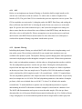


![Audio Extremes Entertainment [Graffiti Spray User Manual]](http://vs1.manualzilla.com/store/data/005858722_1-74e7fc11dae975c9529a69c83302f350-150x150.png)