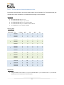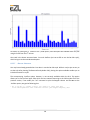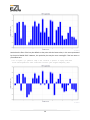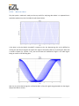
1
EZL USER MANUAL V1.0 CONTENTS 1 WELCOME ..................................................................................................................................................... 4 2 INSTALLATION ............................................................................................................................................... 4 3 OVERVIEW ..................................................................................................................................................... 5 4 DIRECTORY BROWSER ................................................................................................................................... 6 4.1 5 LISTINGS ..........................................................................................................................................................7 COMMAND WINDOW ................................................................................................................................... 8 5.1 5.2 5.3 5.4 VERBOSE MODE ...............................................................................................................................................8 AVAILABLE COMMANDS .....................................................................................................................................8 COMMAND HELP ..............................................................................................................................................9 KEYBOARD SHORTCUTS ......................................................................................................................................9 6 TOOLBOXES ................................................................................................................................................. 10 7 TOOLBAR ..................................................................................................................................................... 10 8 PLOTTING DATA FROM FILES ....................................................................................................................... 13 8.1 USING THE FILE SETUP DIALOG ..........................................................................................................................13 8.1.1 The Key Column......................................................................................................................................15 8.1.2 Reading Dates and Times.......................................................................................................................16 8.2 USING THE COMMAND WINDOW ......................................................................................................................17 8.2.1 The EZL Command – Basic Options ........................................................................................................18 8.2.1.1 8.2.1.2 8.2.1.3 8.2.2 Plotting Multiple Curves ............................................................................................................................... 18 Plotting Multiple Files ................................................................................................................................... 20 Plotting Multiple Curves From Multiple Files ................................................................................................ 21 The EZL Command – Advanced Options.................................................................................................22 8.2.2.1 8.2.2.2 8.2.2.3 8.2.2.4 8.2.2.5 8.2.2.6 8.2.2.7 8.2.2.8 –Date, –Time, and –Datetime ....................................................................................................................... 22 –Spanx and –Spany ....................................................................................................................................... 24 –Limitxmin, –Limitxmax, –Limitymin, and –Limitymax ................................................................................. 25 –Z, –Limitzmin, and –limitzmax..................................................................................................................... 25 –Lookfor ........................................................................................................................................................ 26 –Pntlbl ........................................................................................................................................................... 27 –Bar and –Barfloor ........................................................................................................................................ 28 –Modx and –Mody ........................................................................................................................................ 30 9 COMMAND-LINE PLOTTING ......................................................................................................................... 31 10 LABELING PLOTS .......................................................................................................................................... 31 10.1 CUSTOM LABELS .............................................................................................................................................31 10.2 CUSTOM LINES AND ARROWS ............................................................................................................................32 10.2.1 Text ....................................................................................................................................................33 10.2.2 Text Rotation .....................................................................................................................................33 10.2.3 Text Frame .........................................................................................................................................33 1 10.2.4 11 Changing Arrow Position/Shape ........................................................................................................33 EZSCRIPT ..................................................................................................................................................... 33 11.1 11.2 EZSCRIPT EDITOR............................................................................................................................................33 EZSCRIPT INPUT ARGUMENTS ...........................................................................................................................34 APPENDIX A. DATE/TIME FORMATTING ........................................................................................................... 37 APPENDIX B. EZL COMMANDS ......................................................................................................................... 37 B.1. B.2. B.3. B.4. B.5. B.6. B.7. B.8. B.9. B.10. B.11. B.12. B.13. B.14. B.15. B.16. B.17. B.18. B.19. B.20. B.21. B.22. B.23. B.24. B.25. B.26. B.27. B.28. B.29. B.30. B.31. B.32. B.33. B.34. B.35. FORWARD SLASH (/) ........................................................................................................................................38 ADD, SUB, MUL, DIV, AND ADDX, SUBX, MULX, DIVX ...........................................................................................39 CACHE ..........................................................................................................................................................39 CACHERETRIEVE (OR CACHER) ...........................................................................................................................39 CD ...............................................................................................................................................................40 CLEAR ...........................................................................................................................................................40 CLOSETAB ......................................................................................................................................................40 CROP ............................................................................................................................................................40 DIFF .............................................................................................................................................................40 EXIT..............................................................................................................................................................41 EXPR.............................................................................................................................................................41 EZL ...............................................................................................................................................................41 FOOTNOTE.....................................................................................................................................................41 FUNCTION .....................................................................................................................................................41 HELP ............................................................................................................................................................42 HMARKER .....................................................................................................................................................42 LEGENDPOS....................................................................................................................................................42 LINE .............................................................................................................................................................42 LINEWIDTH ....................................................................................................................................................43 LS ................................................................................................................................................................43 MEAN...........................................................................................................................................................43 MEANAGGR ...................................................................................................................................................43 NEWTAB .......................................................................................................................................................43 NORM ..........................................................................................................................................................43 PNTRAD ........................................................................................................................................................44 PNTS ............................................................................................................................................................44 POLY ............................................................................................................................................................44 PWD.............................................................................................................................................................45 REMOVE........................................................................................................................................................45 RESCALE ........................................................................................................................................................45 SINK .............................................................................................................................................................45 SMOOTH .......................................................................................................................................................45 SORT ............................................................................................................................................................46 SPANX ..........................................................................................................................................................46 SPANY...........................................................................................................................................................46 2 B.36. B.37. B.38. B.39. B.40. B.41. B.42. B.43. B.44. B.45. B.46. STATS ...........................................................................................................................................................46 TITLE ............................................................................................................................................................46 UNDO ...........................................................................................................................................................47 UNWRAP .......................................................................................................................................................47 USINGTAB......................................................................................................................................................47 VERBOSE .......................................................................................................................................................47 VERSION........................................................................................................................................................47 VMARKER .....................................................................................................................................................47 XLBL .............................................................................................................................................................48 YLBL .............................................................................................................................................................48 BACKSLASH (\) ...............................................................................................................................................48 APPENDIX C. WALKTHROUGH .......................................................................................................................... 48 3 1 WELCOME Welcome to EZL! We’re very excited about our latest product and truly hope it lives up to your expectations. If you ever have any questions, concerns, update requests, or simply cannot figure out how to make it do what you need, please do not hesitate to send us a message or call. We look forward to hearing from you. Support: Email: Web: (208) 907-1395 [email protected] www.ezlsoftware.com 2 INSTALLATION Installation of EZL is easy! A lot of effort was made to keep EZL self-contained so that no heavy installation packages are required. EZL can be run from any directory you desire. Just create the directory (if it doesn’t already exist) and place ezl.exe and your license file (ezlicense.lic) within. Typically, we use C:\EZL as the directory, but you can use anything. This manual will assume we are using C:\EZL. To create a shortcut icon on your desktop, simply drag ezl.exe with your right mouse button, from your EZL directory to the desktop. This will open a menu. Select “Create Shortcut Here”. Then right-click the new shortcut, choose Rename, type EZL, and press Enter. It is always a good idea to add your EZL directory to your computer’s system path. This will make the program accessible for command-line usage. This is optional; if you never intend to run EZL from the command-line, this can be skipped. To add EZL to the system path for Windows XP: Click StartControl PanelSystem. On the Advanced tab, click Environment Variables. In the System Variables section, select the variable “Path” and click Edit. At the end of the Variable Value field, type “;C:\EZL” (without the quotes and note the leading semicolon). Then click Ok. Click Ok again. To add EZL to the system path for Windows 7: Click the Windows Button. In the search box, type Environment Variables. Click either “Edit environment variables for your account”, or “Edit the system environment variables”. In the Environment Variables windows, select the “Path” variable. If “Path” cannot be found, create it. Add “;C:\EZL” to the end of the Variable Value field (without the quotes and note the leading semicolon). Then click Ok. Why no installation program? There are many reasons, but here are a few: 4 Portability - EZL can easily be run directly from USB memory. This means you can carry the program with you to run on any system. User Privileged Access - Many office workstations block setup programs from running, for nonadministrator accounts. With no setup required, EZL will run right out of the box. Maintain a Cleaner Computer - No installation means no uninstallation. No residual files, orphaned shortcuts, bad registry entries, etc. 3 OVERVIEW EZL is a scientific graphing and data plotting application, built to simplify your workload. Our primary goal was to ease the task of routine data plotting and analysis. Loading data into EZL is as simple as dragging-and-dropping or double-clicking your data file. The most commonly used functions are at the front of the interface while the more advanced capabilities, such as live data streaming, take just a few mouse clicks. When EZL is first run it will display an interface similar to the one shown below, with 5 primary components. 5 1. Directory Browser The Directory Browser is used to provide a quick and easy way to find and import data files. Use the browser to navigate through your computer to find your data files or scripts. Then simply double-click a file or drag one or more files from the browser onto the Plotter (5) to prompt EZL to plot your data. 2. Command Window The Command Window is used to provide warnings, errors, or information from EZL, or to issue commands to EZL such as to enable markers, show statistics, or remove data. To see a complete list of available commands, type “help” in the command window. To see help on a specific command, type “help <command>”, where <command> is replaced with the name of the command. Example: “help smooth”. To get information on help syntax formatting, type “help help”. 3. Toolboxes The Toolboxes provide a categorized view of the functions available to EZL. Nearly all of the functions contained within the toolboxes have accompanying commands which can be issued through the command window. 4. Toolbar The buttons on the toolbar provide access to important commonly-used tasks. 5. Plotter The central object, the Plotter, provides access to the data plots. Plots are stacked inside the Plotter, with each plot raised by clicking a tab on the tab bar, found on the top of the Plotter. When EZL first opens (as shown above) only a single tab exists, labeled “Plot 1”. Tabs can be relabeled by right-clicking on the appropriate tab label. New tabs can be created, and old tabs removed, by clicking the and buttons on the top-right of the Plotter, respectively. 4 DIRECTORY BROWSER The Directory Browser makes it easy to find data or scripting files on the computer. The default directory (i.e. the path which is automatically loaded when EZL is run) can be set in one of these three ways: 1. From the system menu click FileDefault Directory, then browse to the desired directory. 2. Use the shortcut key sequence: Ctrl+D, then browse to the desired directory. 6 3. From the Toolboxes, click SystemDefault Settings. In the System Settings section, type the desired path into the System Path box. Then click Apply & Save for that item. A green check next to the Apply & Save button will indicate that the new setting was saved. Note that the check does not indicate that the path was valid, only that it was saved to load the next time EZL is run. a. When setting the default directory through the Default Settings page, the Directory Browser does not change to the new directory (as it does by the other two methods). This is by design, not by accident. b. Once you are finished with the Default Settings page, it is hidden (or toggled off) by again clicking SystemDefault Settings in the Toolboxes pane. The Directory Browser’s current directory establishes the workspace path used throughout EZL. In other words, whenever you reference a file, unless you explicitly type the full path, EZL will use the path of Directory Browser’s current directory. Therefore, the current workspace path may be changed three different ways: 1. Navigate to the desired path from within the Directory Browser using the volume selector dropdown box and the parent directory icon in the listings or the parent directory tool button . 2. Browse to the desired path from within the Directory Browser using the Browse tool button . 3. Or, manually specify the path using the “cd” command within the Command Window (eg. cd c:\my data). These methods change your current workspace path, but do not change your default workspace path as described above. As with all windows of the main interface, the Directory Browser is dockable. You can “float” the browser or re-dock it by dragging it out of its current location by grabbing its title. It can also be closed by clicking the X on the top-right of the browser. Once closed, it can be re-opened from the system menu, DockDirectory Browser. 4.1 LISTINGS The listings (i.e. files & directories) in the Directory Browser can be directly renamed, deleted, or moved. Furthermore, files within the listings can be dragged onto the Plotter (or double-clicked) for plotting. Upon doing so, a simple setup dialog is automatically opened which allows you to define the plotting parameters. This setup dialog is discussed in greater detail later. To drag multiple files on to the Plotter, click a file, hold down the Ctrl key on your keyboard, and then click additional files. Once all the files are selected simply drag one of the selected files on the Plotter – it will be accompanied by the other files in the selection. You may also use the Shift key, which will select all files between (and including) the first and last files clicked. 7 EZScripts (EZL scripts are denoted with .ezs file extensions) are displayed in the listing with the EZL logo, for easy recognition. EZScripts are discussed in greater detail later. Sometimes a file(s) may appear to be absent from the listing, for example if a new file was created from outside of EZL. The listing may be repopulated using the Refresh tool button . To view the contents of a file (for all files but EZScripts) simply right-click the file and select View from the displayed menu. EZScripts are viewed by right-clicking the script and selecting Edit. This will open the script in EZL’s built-in EZScript Editor. 5 COMMAND WINDOW The Command Window is used to provide feedback (warnings, errors, or information) from EZL to you and to issue commands from you to EZL. Commands exist to provide quick access to the functions within EZL. Typing commands is often easier and faster than finding them in the Toolbox pane or Toolbar. Furthermore, commands can be stored in text files and saved with .ezs extensions to create EZL scripts. 5.1 VERBOSE MODE To enable verbose messaging, type “verbose” and press enter. The “verbose” command toggles verbose mode on and off, or it can be explicitly enabled or disabled via commands “verbose on” and “verbose off”, respectively. 5.2 AVAILABLE COMMANDS At the current software version (v1.0.1) the following commands are available through the Command Window or EZScripts: 1 / Cd Div Footnote Line Mul Pnts Sink Stats Unwrap Xlbl Add Clear Divx Function Linewidth Mulx Poly Smooth Sub Usingtab Ylbl Addx Closetab Exit Help Ls Newtab Pwd Sort Subx Verbose 1 \ Cache Crop Expr Hmarker Mean Norm Remove Spanx Title Version Cacher Diff Ezl Legendpos Meanaggr Pntrad Rescale Spany Undo Vmarker 1 While the first and last items, “/” and “\”, are not commands (they are used for EZL text formatting), they are provided here as they do have in-program help contexts. 8 For detailed descriptions of the commands, refer to Appendix B of this manual. 5.3 COMMAND HELP EZL provides in-program help on its commands. Typing “help” in the Command Window will return a list of available commands. For help on a specific command, type “help [command]”, where [command] is replaced with the command of interest. Example: Command Window ----------------------------> help title > Format : Title [label] Purpose : Sets the title for the plot currently in view. Calling title with no label sets an empty title (ie. removes the title). Example : "title Ramsey Fringes" Notes : Labels can be multi-line by inserting \n within the label to indicate a line break. EZL includes a set of special characters available for use in labels. Type "help /" for a display of the character set. > The Help system uses the following conventions: Quotes (“) are to be ignored, except where noted. For example, in the description above, “help [command]” means to type the syntax within the quotes, excluding the quotation marks themselves. All commands are case-insensitive. Typing “help ADD” is the same as typing “help add”. Less-than/greater-than symbols < > denote mandatory parameters. Brackets [ ] denote optional parameters. Braces { } denote an enumerated list of parameters. o Mandatory lists will therefore be presented as < { } > o And optional lists as [ { } ] Typing “help help” in the Command Window will elaborate on the Help system’s syntax convention discussed above. 5.4 KEYBOARD SHORTCUTS The Command Window has the following keyboard shortcuts: Up-arrow/Down-arrow – Use the keyboard up/down arrow keys to scroll through the commands which have recently been issued. The history has a depth of 20 commands. Tab – Use the tab key to auto-complete partially entered file/path names. For example, suppose your workspace contains files “datafile1.dat”, “datafile2.dat”, and “datafile3.dat”. If you type “data” into the Command Window and press tab, “data” will change to “datafile1.dat”. Pressing tab again will change it to “datafile2.dat”. Tab again will change it to “datafile3.dat”, and then 9 back to “datafile1.dat”. If the file/path you are auto-completing contains a space (eg. “c:\my path\data file.dat”) the auto-complete will only work if you add a quote (“) in front of the syntax, before pressing Tab. Examples: o ezl –f datafile| (pressing tab at the | will auto-complete) o ezl –f “c:\my path\data file| (pressing tab at the | will auto-complete) o ezl –f c:\my path\data file| (pressing tab at the | will fail to auto-complete without the quote, because of the spaces in the path) Ctrl+C – Use this to copy one or more lines from the Command Window. Select the lines you wish to copy then press Ctrl+C on the keyboard. If no text is selected, Ctrl+C acts as a command abort. In this case, any text currently entered will be ignored and the cursor will move to a new line. Note that Ctrl+C does not act as a process abort. Ctrl+V – Paste the text saved to the clipboard (via Ctrl+C). If multiple lines are copied to the clipboard and then pasted using Ctrl+V, the commands are executed line-by-line as they arrive. 6 TOOLBOXES The Toolboxes provide a categorized view of the functions available to EZL. Nearly all of the functions contained within the toolboxes have accompanying commands which can be issued through the command window. The items contained in the Toolboxes panel will be discussed throughout this manual. 7 TOOLBAR Cache – This button allows you to manually cache (store in memory) the current data set, providing you with a backup for later re-use. This can be a great time-saver in the event of mistaken data operations - accidental over-smoothing, for example. You should try to get in the habit of caching your data before performing operations. Doing so will spare you the frustration of having to rework your steps if you’re involved in a lengthy process and make a mistake. The cache is automatically initialized when you first load a data file. So if you do forget to cache your data, you can always revert back to the original state. Clicking the cache button will provide a submenu with options to either cache the current data set or to retrieve an existing data set. The cache has storage for only one data set. Caching a data set will replace the existing set, if one already exists. The equivalent command is “cache” to store data, and “cacheretrieve” (or “cacher” for short) to retrieve stored data. 10 Statistics – Clicking this button will compute a set of common statistics for all the curves in the currently active plotter. The results will be displayed in the Command Window. The equivalent command is “stats”. Trim Outliers – This button is used to automatically remove data outliers. Outlier determination is based on the standard deviation of the data. With a curve plotted, clicking this button will present a submenu with the following options: 1, 2, 3, and n. Selecting one of these will remove all points with absolute values which exceed 1 standard deviation, 2 standard deviations, 3 standard deviations, or n standard deviations from the mean, respectively. Choosing n allows you to specify a value for n. If verbose-mode is enabled the statistical results will be displayed in the command window. Example: > C1: σ = 1.0008, μ = 0.000404752, Upper Bound = 1.0012, Lower Bound = -1.00039 C1 Trimmed: 317138 points (31.714%). Total trimmed: 317138 points (31.7138%). When multiple curves are plotted, the Trim Outliers button will allow you to operate on each curve independently or to treat all curves as a single data set. In the latter case, the standard deviation and mean calculations will include all data from all plotted curves and will remove points based on those values. Example: > Concatenated data: σ = 0.98657, μ = 0.0012, Upper Bound = 0.9873, Lower Bound = -0.9851 C1 Trimmed: 161274 points (32.339%). C2 Trimmed: 160469 points (32.176%). Total trimmed: 321743 points (32.2573%). The equivalent command is “trimoutliers” (or “trim” for short). Crop Tool – This button toggles the crop mode on or off enabling you to manually trim outliers or discard unwanted data points. When this mode is off, using your mouse to draw a box around a selection of data zooms-in on the data. This is done internally by changing the x and y-axis scales to the dimensions represented by the top-left and bottom-right corners of the drawn box. The data which is no longer visible (i.e. points which are outside of the new scale) are not thrown away; they still exists for all operations and statistical calculations, they are simply no longer in view. However, when the crop mode is on the act of drawing a box around data (we call this “drawing a rubber band”) does discard all data which falls out of view. This tool is therefore very useful for quickly removing unwanted data points, or for shortening large data sets. Simply draw a rubber band around the data you wish to keep; everything outside of the rubber band is removed and the plot automatically rescales. 11 Note that when you click on the plot to begin drawing a rubber band, and crop mode is on, a scissors icon will follow the mouse pointer to remind you that you are in fact in crop mode, and not zoom mode. If you mistakenly crop data where you intended to zoom, type “undo” or click the undo button. Eraser Tool – The eraser tool is the counter-part to the crop tool. In this mode, all data points encapsulated by the rubber band are discarded and points outside the rubber band are retained. So, it behaves in a manner opposite of the crop tool. Selection Tool – The selection tool is mix between the crop tool and the eraser tool. Drawing a rubber band around a section of data will remove the encapsulated data points from their parent curve, but instead of discarding the points, they will form a new curve. Undo – EZL provides you with two types of data caches: the User Cache, which is accessed by you (via the Cache toolbar button, or the “cache” command), and the Auto Cache, which is automatically populated whenever you perform an operation which modifies the current data set. As is the case with the User Cache, the Auto Cache is only one deep. Unlike the User Cache, the Auto Cache is emptied upon retrieval thus restoring the used memory back to the program. The equivalent command is “undo”. Snap-To – This toggle button becomes available when mouse pointer tracking (accessed by going to ToolboxesPointer) is enabled. Mouse tracking displays the coordinates of the mouse pointer’s position within the plot. When this mode is off the displayed coordinates do not necessarily correspond to any particular point within the plotted data curves, but only to the plot’s coordinate system itself. However, when this button is toggled on, the displayed coordinates will snap to the curve’s point which is closest to the pointer’s current position. An animation will hover over the chosen point, to indicate which coordinate is being display. If more than one curve is plotted, you will be asked to choose the curve of interest upon enabling this feature. In order to find the point closest to the mouse pointer, EZL must convert every data point to corresponding pixel locations and then compute Pythagorean distances from the current mouse position to each of the locations. And it must do this for every movement of the mouse. This is a computationally expensive procedure. Therefore, for very large data sets you may experience lag in graphics refresh. 12 Rescale – This button provides a convenient way to rescale the plotter to show all the plotted data. It essentially removes any zoom settings or mouse-wheel scrolls. The equivalent command is “rescale”. Zoom-In – Each time a rubber band is drawn to zoom in or out, the resulting zoom span and range (zoom setting) is saved for later reuse. This button becomes available when a zoom-in setting is available. - Zoom-out – As with the zoom-out button, this button becomes available when a zoom-out setting is available. Abort – The Abort toolbar button is displayed during Allan Deviation computations. Because the Allan Deviation is a CPU intensive algorithm (for All Tau calculations) it can take quite a while for large data sets. This button stops the calculation and displays any results which were computed prior to the abort. Future versions of EZL will use this button for other potentially long wait-time processes, such as data file loading. 8 PLOTTING DATA FROM FILES With EZL there are multiple ways to plot data from files. This section discusses these methods. 8.1 USING THE FILE SETUP DIALOG The File Setup Dialog provides a simple way to load and configure data from data files. To use the File Setup Dialog, browse to the file you wish to plot using the Directory Browser, and then double-click the file or drag it onto the Plotter. The File Setup Dialog will be displayed automatically. An example is shown below. 13 The panel on the left contains a listing of the files to be plotted. The example shows only a single file; to load multiple files into the dialog, simply select all the desired files (using the Shift and/or Ctrl keys on your keyboard) from within the Directory Browser, and then drag them onto the Plotter. When configuring multiple files, the settings for each file are displayed by clicking on the file names in the panel on the left. For each individual file, the File Setup Dialog parses a sample of its contents and places the sample into a preview table on the bottom (as shown). Choose the desired x and y data columns from the dropdown boxes above each table column. If you wish to have no x-axis column, change the default selection to “-“. Enter any scaling factors for the x and y axis columns into the appropriate fields of the top-left tabbed control box. If your file begins with comment lines which need to be ignored, or you wish to begin your data plot at some midpoint within the file, enter the number of lines to be skipped using the Skip field in the “Other Options” section. You can then repopulate the table if desired, by clicking the Reload button. Doing so will extract the 15 lines which directly follow the line number indicated in the Skip field. You may also use the reload button to repopulate the table if the file is modified externally to EZL. The Get field is used to instruct EZL to plot only a certain number of data points from the file. As an example, suppose you have a million-point data file and you want to plot the data from lines 500,000 to 600,000. In this scenario you would set the Skip field to 499,999 and the Get field to 100,000. 14 The Header field is used to specify a header row, should your data file contain one. In the example figure above, our field has a header at the first row. It is important to know that the Header parameter always precedes the Skip parameter. For example, if your file contains 9 lines of comments followed by a header row, you would set Header to 10 and Skip to None because the 9 comment lines will be bypassed to get to the header row on the 10th line. Or suppose your file contains 10 comment lines where the 4th line is actually a header row. In this case you would set Header to Row 4 and Skip to 6 to skip the remaining unnecessary comment lines before getting to the first data row. Above the Ok button on the right is an Append checkbox. If you are plotting to a Plotter which already contains data curves, use this checkbox to add (or “append”) the new data curves to those which already exists. Checking this box will keep the existing curves in place and unmodified. Leaving the box unchecked, however, will replace all existing curves with the new curves generated from the files in the File Setup Dialog. Upon clicking Ok, the resulting plot command is printed to the Command Window and executed. To repeat or modify the plot command, simply press the up arrow on your keyboard to retrieve the command from the command history. 8.1.1 THE KEY COLUMN One of EZL’s advanced plotting features is the Key parameter. The Key parameter specifies a column that contains information which disambiguates curves within a given file. As an example, consider the data shown in the File Setup Dialog below. 15 As shown, this particular file contains a mix of data points, half of which contain data points corresponding to measurements of “Car3” and the other half of “Car4”. By designating this column to be a Key column, EZL will know to separate the data points into unique curve sets as it parses the file. The plot resulting from this example is shown below. 8.1.2 READING DATES AND TIMES When the data in the input files are time-stamped with dates and/or times, the time-stamp columns may be identified by selecting “date”, “time”, or “datetime” from the drop-down box above the preview table. Selecting these options will present corresponding tabs to input their formatting. An example is shown below. 16 Because time-stamps come in many different forms, EZL allows you to build your own format using time and date specifiers. In the example above, the date is formatted as “%Y-%m-%d”. As you enter your specifiers, an example of a formatted date/time, as represented by your format string, will be dynamically displayed in the tab. Several commonly used formats are pre-loaded into the Format box. You can choose one of the pre-loaded formats, or build your own. A table describing all available format specifiers is provided in the Appendix of this manual. In the example above, the input file has its date and time separated into two columns. This does not have to be the case. For instance, suppose our time stamp is ISO-8601 formatted, such as “2013-0826T01:05:58Z”. In this case, we will select “datetime” for the appropriate column and change our Format to: %Y-%m-%dT%H:%M:%SZ. At other times, the date and time may span multiple columns, such as: Mon, 26 Aug 2013 01:05:58. In this case we can either select this to be a datetime and format it all at once, or as a date and time pair. Choosing the former, our format specifiers would look like this: “%a, %d %b %Y %H:%M:%S”. Important: In cases such as this, where commas are included in the time-stamp, the commas will not be visible in the preview table, as commas (like spaces) are inherently used by EZL as column delimiters. However, if they exist the commas must be included among the specifiers when formatting the timestamp. In cases like this, it can be helpful to view the raw data. To do so, right-click on the file within the Directory Browser, and click View. When parsing data files which contain dates and/or times, EZL converts all time-stamps to decimal Modified Julian Date (MJD) values for plotting. The plotted results are therefore shown as MJD values along the x-axis. To convert these values to ASCII dates and times, open the Grid Adjustments category in the Toolboxes pane, and select MJD->Date/Time. Any errors in parsing the time-stamps will be displayed in the Command Window. If errors occur, you may either reopen the File Setup Dialog as before, or press the up arrow on your keyboard to edit the plot command. Press enter to then accept and execute the modified command. 8.2 USING THE COMMAND WINDOW Data files can be plotted via the Command Window, using the “ezl” command. In fact, this is how the File Setup Dialog (described above) operates. The File Setup Dialog is simply a graphical entry form which uses your input to build an “ezl” command. The resulting command is sent to the Command Window for execution. Bypassing the dialog, and entering the command manually, or saving them to EZScripts for later repeated execution, often saves you time. Finally, the “ezl” command has options not available through the File Setup Dialog, which offer additional plotting flexibility and functionality. 17 8.2.1 THE EZL COMMAND – BASIC OPTIONS The “ezl” command is used to load and plot data files. The file import, data preprocessing, and plot configurations are passed to the “ezl” command via input options. Options begin with a minus sign and are followed by an argument which contains one or more fields. Options syntax: -option field1 field2 … fieldn The –f option is used to specify the name of the file to plot. The x and y-axis columns are passed in as –x and –y, respectively. Therefore, the command > ezl -f file.dat –x 2 –y 3 will plot data from the file “file.dat” using the file’s second column for the x-axis and the file’s third column for y. The default value for –x is 1 and the default value for –y is 2. Therefore, if you are plotting column 2 versus 1 you can shorten your command to > ezl -f datafile.dat Specify –x 0 to use no x-axis column from the input file. In this case, EZL will use a data point counter for the x-axis values, starting at 0. Arithmetic operations may be performed on the x and y column(s) using options –addx <value>, −subx <value>, –mulx <value>, and –divx <value> for the x-axis column, and –add <value>, –sub <value>, −mul <value>, and –div <value> for the y-axis column. For instance, to scale our above example by 2 and then add 0.5 we could issue: > ezl –f file.dat –x 2 –y 3 –mul 2 –add 0.5 Note, to ease memorization the –mul and –mulx options are also accepted as –mult and –multx. Additionally, the y-axis arithmetic options (–add, –sub, –mul, and –div) can be provided as –addy, –suby, −muly (or –multy), and –divy. The order of the options within the “ezl” command does not matter. So, > ezl –f file.dat –x 2 –y 3 –mul 2 –add 0.5 > ezl –f file.dat –y 3 –x 2 –add 0.5 –mul 2 > ezl –y 3 –x 2 –add 0.5 –mul 2 –f file.dat all result in the same plot. 8.2.1.1 PLOTTING MULTIPLE CURVES Multiple columns can be read in from the input file by appending additional fields to the –y option. For instance, to plot columns 2 and 3 versus an x-axis defined by column 1 we can issue this command: > ezl –f file.dat –x 1 –y 2 3 18 or equivalently (since the default of –x is 1) > ezl –f file.dat –y 2 3 There is no limit to the number of columns which may be added to the –y option. As before, the data can be preprocessed with arithmetic options: > ezl –f file.dat –y 2 3 –sub 5 2.5 While the order of the options within the “ezl” command does not matter, the order of the fields within any particular option does! Notice that for this example, the arithmetic option passes two fields (5 and 2.5). The first field value (5) applies to the first y-axis column (2) and the second field (2.5) applies to the second column (3). > ezl –f file.dat –y 2 3 –sub 5 2.5 When there are not enough arithmetic fields to satisfy each of the column fields, the last arithmetic field propagates forward. This means that if you wish to apply the same value to all data columns, you need only to pass the value once; you are not required to pass the same value for every column. > ezl –f file.dat –y 2 3 –sub 5 As another example, suppose we are plotting many columns, say 2, 3, 4, 8, and 12, and we want to subtract a value 5 from the first two columns (2 & 3) and subtract 2.5 from the remaining columns. > ezl –f file.dat –y 2 3 4 8 12 –sub 5 5 2.5 Notice that the field which is propagated is that which is last entered, 2.5 in this example. As a final example, suppose we wish to subtract 2.5 from column 12 and subtract nothing from the other columns. This can be accomplished by either of the following commands: > ezl –f file.dat –y 2 3 4 8 12 –sub 0 0 0 0 2.5 > ezl –f file.dat –y 12 2 3 4 8 –sub 2.5 0 The second command shortcuts the syntax of the first by changing the position of column 12 in the –y listing, thereby allowing the –sub 0 to propagate. However, there is a difference between these two commands. Because the second command places column 12 at the top of the order, column 12 will be the first curve plotted. The plotted curve of column 12 will then be followed by plots of columns 2, 3, 4, and 8. Therefore, the plotted curve of column 12 will be “underneath” the remaining curves. This is an important feature to understand as it affects the presentation of your data. Changing the order of your −y fields gives you the ability to control the plotted order of your curves. While expected in future 19 versions, the current version of EZL has no method to adjust the order of your curves once they are on the Plotter. 8.2.1.2 PLOTTING MULTIPLE FILES Multiple files may be plotted by either listing all input files with a common –f, or by using multiple –f’s. The following two commands are identical; they both load two files and plot column 2 versus 1 from each file. > ezl –f file1.dat –f file2.dat > ezl –f file1.dat file2.dat This syntactic flexibility is offered to provide improved readability in EZScripts, as discussed later in this manual. The files may be listed individually, as they are above, or they may be input using regular expressions (see http://en.wikipedia.org/wiki/Regular_expression). For instance, all of the following commands will yield the same result: > ezl –f file1.dat –f file2.dat > ezl –f file1.dat file2.dat > ezl –f file[12].dat Use the wildcard * in a filename to match zero or more additional characters. For example “file*.dat” will match file.dat, file1.dat, file2.dat, file_anything_.dat, etc. Similar to the manner in which we assign arithmetic options to input columns (as discussed in section 8.2.1.1), we assign input columns to files by supplying corresponding column options. Consider the following example: > ezl –f file1.dat file2.dat file3.dat –x 1 -y 2 -x 2 -y 5 Notice that the first column options apply to the first file and the second column options apply to the second file. Also notice that, as there are no column options explicitly stated for the third input file, the third file assumes the last columns specified. In general, for each option passed to the “ezl” command, the default for that option is updated to the last entry of its type. This is true for column options and arithmetic options alike. Also notice that, in the example above, there are in fact two unique –y entries; the columns 2 and 5 are not bundled together as fields of the same –y option. Indeed “–y 2 –y 5” and “–y 2 5” are two very different things. The first statement says “use column 2 from the first file, use column 5 from the second file”. The latter statement says “use columns 2 and 5 from the first file” and since no direction exists for the second file, columns 2 and 5 are used from it as well. Therefore, “–y 2 –y 5” will result in two total plots, whereas “–y 2 5” would result in four. 20 8.2.1.3 PLOTTING MULTIPLE CURVES FROM MULTIPLE FILES By combining the information in the two sections above we can formulate “ezl” commands which plot multiple curves from multiple files. Let’s demonstrate through a set of examples: Commands 1. 2. 3. 4. 5. ezl –f file1.dat file2.dat –y 2 5 –y 2 ezl –f file1.dat file2.dat –y 2 5 –y 2 –mul 5 ezl –f file1.dat file2.dat –y 2 5 –y 2 –mul 5 –mul 1 ezl –f file1.dat file2.dat –y 2 5 –add 10 –sub 0 –sub 0 10 ezl –f file[12].dat –y 2 5 –add 10 –add 10 0 Resulting Plots Command File 1 2 3 4 5 Column Add Sub Mul Div file1.dat 2 0 0 1 1 file1.dat 5 0 0 1 1 file2.dat 2 0 0 1 1 file1.dat 2 0 0 5 1 file1.dat 5 0 0 5 1 file2.dat 2 0 0 5 1 file1.dat 2 0 0 5 1 file1.dat 5 0 0 5 1 file2.dat 2 0 0 1 1 file1.dat 2 10 0 1 1 file1.dat 5 10 0 1 1 file2.dat 2 10 0 1 1 file2.dat 5 10 10 1 1 file1.dat file1.dat file2.dat file2.dat 2 5 2 5 10 10 10 0 0 0 0 0 1 1 1 1 1 1 1 1 Explanations 1. Using the default x-axis column (–x 1), this command applies –y 2 5 to file1.dat and –y 2 to file2.dat. Therefore, this command creates three total plots. 21 2. 3. 4. 5. 8.2.2 Same as above but now there is a –mul 5 which is applied to the fields of the first –y option (-y 2 5). But because there are two fields in the –y option and only one field in the –mul option, the 5 in the –mul option is propagated to the second –y field (see 8.2.1.1). As –mul 5 is the last specified option of its kind, it becomes the -mul default (8.2.1.2) and is now applied to the second –y option (–y 2). Same as above but now we have supplied two –mul options, one for each of our –y’s. The first –mul applies to the first –y (which applies to the first file as before). The second –mul entry (–mul 1) applies to the second –y (–y 2) which applies to file2.dat. A bit more complicated, here we have the same two input files with a default to plot columns 2 and 5 from each file. Notice that the entire –y option becomes the default, not just the final field of the option. Therefore –y 2 5 applies to the first file (file1.dat) and, as –y 2 5 is now the default, applies also to the second file (file2.dat), resulting in 4 total plotted curves. Next we consider the arithmetic options –add 10, −sub 0, and –sub 0 10. As there is only one –add stated, it becomes the default and 10 is added to all columns for each file. Then, there are two –sub options. The former applies to the first –y option (which applies to the first file) and so 0 is subtracted from both input columns of file1.dat. The latter (–sub 0 10) applies to the second –y option which, while not explicitly stated, is implied by the default –y 2 5 and so 0 is subtract from column 2 of file2.dat and 10 is subtracted from column 5 of file2.dat. th th While the syntax of the 5 command is quite different from that of the 4 command, the net result is the same. Here we succinctly specify the two input files, file1.dat and file2.dat, through the use of a regularexpression. The –y columns 2 and 5 are applied to each file, the value 10 is added to column 2 of file1.dat and is propagated for addition to column 5 of file1.dat. Then, via the second –add option (−add 10 0), the value 10 is added to column 2 of file2.dat and 0 is added to column 5 of file2.dat. THE EZL COMMAND – ADVANCED OPTIONS In addition to the options discussed above, the “ezl” command supports several advanced options. 8.2.2.1 –DATE, –TIME, AND –DATETIME When your data is time-stamped with ASCII characters which are not directly plottable, such as “June 13, 1975” or “06/13/75”, the –x option can be replaced with –date, –time, or –datetime to specify columns which contain date strings, time strings, or date/time strings, respectively. The –date and −time options may be used simultaneously in an “ezl” command, but both options are mutually exclusive with the –datetime option. It makes no sense to use both –datetime and –date, for example. Let’s see how this works. Assume we have a data file (time_series.dat) comprised of the following content: 2013-08-26 2013-08-26 2013-08-26 2013-08-26 2013-08-26 2013-08-26 2013-08-26 … 01:05:58 01:07:24 01:08:51 01:10:17 01:11:44 01:13:10 01:14:36 0.0125357 0.0466993 0.3763479 0.2396948 0.3918675 0.5206156 0.3438054 We can plot this file with the following command: > ezl –f time_series.dat –date 1 –time 2 –y 3 Doing so results in the plot shown below. 22 Notice that the values along the x-axis have been converted from the ASCII date and time values (as read from the data file) to the default timescale of EZL, Modified Julian Date (MJD). The MJD values may be displayed as ASCII date/time values once the data has been plotted, by clicking Grid Adjustments”MJD -> Date/Time” from within the Toolboxes panel. But how does EZL know how to read the data file’s dates and times? How does it know what date and time formats should be used? It doesn’t. The dates and times in the example data above happen to be formatted using EZL’s default date and time formats: Year-month-day (YYYY-mm-dd) and hour:minute:second (HH:MM:SS). Chances are good that your date and time formats will differ. Date and time formats may be passed to the “ezl” command using options –dateformat, -timeformat, and –datetimeformat. Each of these options must then be followed by a format string. Date/time format strings contain specifiers which you use to define your dates and times. A complete list of date/time specifiers is provided in Appendix A. Using the specifiers, your can construct your own date and time formats. Below are several examples: Example 1 Data file content 2013-08-26 01:05:58 0.0125357 2013-08-26 01:07:24 0.0466993 2013-08-26 01:08:51 0.3763479 > ezl –f datafile.dat –date 1 –dateformat %Y-%m-%d –time 2 –timeformat %H:%M:%S –y 3 Or > ezl –f datefile.dat –datetime 1 –datetimeformat “%Y-%m-%d %H:%M:%S” –y 3 Notes The timestamps in data can be represented by formatting the date and time columns individually (as shown in the first command), or by formatting both columns using a single datetime field (as shown in the second command). In the latter case, note that the –datetime 1 option indicates that the field begins with the 1st column. It then extends to the 2nd column, where the two columns are separated by a space. Whenever your format specifiers 23 include a space, you must wrap the entire format in quotes, as shown. The y-column remains as 3, even though the first two columns are included as parts of the datetime field. Example 2 Data file content 2013-08-26T01:05:58Z 0.0125357 2013-08-26T01:07:24Z 0.0466993 2013-08-26T01:08:51Z 0.3763479 > ezl –f datafile.dat –datetime 1 –datetimeformat %Y-%m-%dT%H:%M:%SZ –y 2 Notes For this example, where the data file contains timestamps given in the ISO-8601 format, the only appropriate option is to –datetime, as there exist no column delimiters separating the dates and times. Note that while the format’s Z (for Zulu) must be accounted for within the −datetimeformat specifier string (as it is in the example), the Z is ignore by EZL as an actual time-zone. EZL always assumes times are provided as UTC, irrespective of any provided time-zone designators. Example 3 Data Mon, Mon, Mon, file content 26 Aug 2013 01:05:58 GMT 0.0125357 26 Aug 2013 01:07:24 GMT 0.0466993 26 Aug 2013 01:08:51 GMT 0.3763479 > ezl –f datafile.dat –date 1 –dateformat “%a, %d %b %Y” –time 5 –y 7 Or > ezl –f datafile.dat –date 1 –dateformat “%a, %d %b %Y” –time 5 –timeformat “%H:%M:%S” –y 7 Or > ezl –f datafile.dat –datetime 1 –datetimeformat “%a, %d %b %Y %H:%M:%S” –y 7 Notes This example is similar to those above, but here we show off some of the fancier formatting specifiers. Note again that the timezone designator (here “GMT”) is ultimately ignored as EZL always assumes input time-zones are given in UTC. In this case the GMT field is excluded altogether from the format string, as the field is automatically portioned off into an unused column by its preceding space delimiter. Notice that the first example command does not include a time format string (i.e. there is no –timeformat option). This command is relying on the default time format. In all cases the data column (7) is fixed, regardless of how we bundle together the date and time columns. 8.2.2.2 –SPANX AND –SPANY By default, EZL automatically sets the domain and range axes to tightly encompass the plotted data. For instance, if you are plotting data from 10 to 100, the x-axis grid will start at 10 and end at 100. However, you may change this by manually changing the plot spans using –spanx and –spany. These options must be followed by low and high span values. For example > ezl –f datafile.dat –spanx -50 50 –spany 20 250 24 The –spanx and –spany options need not be used as a pair. In other words, you may use either –spanx or –spany, or both, as you desire. These options only change the viewport of the data. Data points which exist outside of the spans are not removed from the data sets. They still exist and will be included in any calculations or statistics performed on the data. As an alternative to passing these options directly to the “ezl” command, they may be set at any time after the data is plotted by issuing them as commands directly to the Command Window. Example: > ezl –f datafile.dat > spanx -50 50 > spany 20 250 Once a span is set, the span range is fixed as a hard limit to the plotter; clicking the Rescale button (Section 7. Toolbar) to remove any zoom states will rescale the plotter again using your fixed span limits. To remove the span limits issue the command “spanx auto” or “spany auto”. 8.2.2.3 –LIMITXMIN, –LIMITXMAX, –LIMITYMIN, AND –LIMITYMAX These options are used to filter out data points as they are read in from a file. Each option must be followed by a single value. As EZL reads each data point from a file, the point is first scaled by any arithmetic options and the result is then checked against the limits set by these options. If the scaled point exceeds the limits set by these options, either in the abscissa or the ordinate, it is discarded. > ezl –f datafile.dat –limitxmin -50 –limitymax 250 8.2.2.4 –Z, –LIMITZMIN, AND –LIMITZMAX As an extension of the x and y limit options (8.2.2.3), the “ezl” command offers the ability to further restrict data input based on a 3rd column, denoted the z-column. Although the z-column is not, strictlyspeaking, used as an axis for plotting, it can be used as a filter for those which are. The column is defined using the –z option (followed by a valid column number), and its limits are set using –limitzmin and −limitzmax, both followed by a limit value. While parsing the data file, EZL will check the value contained in the designated z-column against the z-limits and will remove the associated x,y data point wherever the z-column value exceeds its set limits. As an example, assume the command > ezl –f datafile.dat –y 2 3 –header 1 produces the following plot: 25 Now suppose we wish to plot only the portions of the sin wave where the tan signal is greater than 0. We can accomplish this by treating the tan data (column 3) as a z-column, and impose upon it a minimum limit: > ezl –f datafile.dat –y 2 –z 3 –limitzmin 0 –spany -3.1416 3.1416 –header 1 It is worth noting that the use of the –spany option in the above command was not required for the operation of the z-column filtering. We include it here only to force the ordinate scale of the plot to be consistent with the prior sin/tan plot. 8.2.2.5 –LOOKFOR The –lookfor option can be used to “look for” a particular string in each data row while parsing the input file. If the row contains a match, the row will be used; if the string is not found in the row, the row will be ignored. For example, suppose we have a file (called racecar_velocities.dat, reusing our example from 8.1.1) with the following contents: 26 Time(s) 0.00000 0.00000 0.00011 0.00011 0.00023 0.00023 … Velocity(mph) 0.000 0.000 0.002 0.011 0.005 0.023 Car_ID Car3 Car4 Car3 Car4 Car3 Car4 In 8.1.1 we used this file to illustrate the use of the –key (or –k) option which, when applied to column 3, separated the data rows into unique curves identified by the text of column 3. Suppose instead, we wish to plot only the rows associated with “Car3”. To do so we can issue the following command: > ezl –f racecar_velocities.dat –header 1 –lookfor Car3 8.2.2.6 –PNTLBL The –pntlbl (point label) option may be a rarely used feature, but it can sometimes provide you with attractive plots. The best way to describe this option is with an example. Suppose we have a file called acq.dat, with the following context: Ch 1 2 3 4 5 6 7 8 9 10 … 30 31 32 Acq 20.349 18.297 64.088 15.609 17.674 11.322 52.658 18.334 16.353 18.429 Doppler Lbl -600.0 PRN1 +3000.0 PRN2 +3400.0 PRN3 -2600.0 PRN4 +3400.0 PRN5 +2200.0 PRN6 -5000.0 PRN7 -4000.0 PRN8 -3000.0 PRN9 +1800.0 PRN10 14.988 -2000.0 PRN30 17.442 -2200.0 PRN31 13.517 -3000.0 PRN32 This particular file was captured from a software GPS receiver after searching the sky for available GPS satellites (denoted PRN1, PRN2, …, PRN32). The 1st column is the receiver’s channel number, the 2nd column is the received signal strength, and the 3rd column is the signal’s offset Doppler frequency. The 4th column was added to the file for the purpose of this example, and will allow us to use the –pntlbl option to label the plotted points. Issuing the command > ezl -f acq.dat -pntlbl 4 –skip 1 -bar -barfloor 0 -spanx 0 33 -spany -3 100 -title "GPS Acquisition" −xlbl "Satellites in View" -ylbl "Signal Strength" results in the following plot: 27 As shown, by passing the 4th column to the –pntlbl option, each data point was labeled within the plot using the texts from the 4th column. Also used in the above command were –bar and –barfloor (to instruct EZL to use the Bar Plot style), which brings us to the next advanced option. 8.2.2.7 –BAR AND –BARFLOOR You may have already guessed what –bar does: it sets the Bar Plot style. While it may be just as easy to set the style after plotting (ToolboxesPlot StyleBar Plot), having the option available enables you to include the switch in scripts. The accompanying –barfloor option, however, is not currently available within the GUI. This option allows you to set the focal point from which the bars extend. Returning to the GPS acq.dat file of the previous section, if we modify the “ezl” command to plot the Doppler column and do not set the −barfloor option, we get the following plot: > ezl -f acq.dat -y 3 -pntlbl 4 -skip 1 -bar -spanx 0 33 -spany -6000 6000 -title "GPS Acquisition" -xlbl "Satellites in View" -ylbl "Doppler Frequency (Hz)" 28 Notice that the floor of the bar plot defaults to the point with the lowest value, in this case represented by the point labeled PRN7. However, this particular plot may be more meaningful if the bars were to pivot about zero: > ezl -f acq.dat -y 3 -pntlbl 4 -skip 1 -bar –barfloor 0 -spanx 0 33 -spany -6000 6000 -title "GPS Acquisition" -xlbl "Satellites in View" -ylbl "Doppler Frequency (Hz)" 29 8.2.2.8 –MODX AND –MODY The plot options –modx and –mody can be very useful for analyzing data where it is expected that a repetitious pattern may exist. Consider the plot shown below: Is the data in this plot ideally sinusoidal? It appears to be, but determining this can be difficult by viewing this plot alone. Suppose we expect this signal to be exactly 10Hz. By re-plotting the data with a -modx 0.1 option (i.e. 1/10Hz = 0.1s), we can see how well matched the signal is to a 10Hz signal. Doing so results in the following plot: Now it is very clear that the signal is not fixed at 10Hz. In fact, this signal was generated as a chirp signal, swept from 10Hz to 10.1Hz. 30 9 COMMAND-LINE PLOTTING Running EZL from a Windows/Linux command line (terminal), as opposed to double-clicking a desktop icon, allows you to pass in arguments to construct initial plots. In this way, you can readily use EZL in your native OS scripts, or even from your own application code. All of the options and “ezl” command rules defined in Section 8.2 are directly applicable. 10 LABELING PLOTS In EZL customizing the primary labels on a plot is easy. The primary labels, including the Title, X-Axis, YAxis, and Footnote (bottom-right) can be changed simply by clicking them. To remove a label, click it, delete its text, and press Ok. To add the label back again go to ToolboxesPlot Annotations and select the appropriate label from the list. Alternatively you may use a command: “Title”, “Xlbl”, “Ylbl”, or “Footnote” (all case-insensitive). For example: > title > title Welcome to EZL In the examples above, the first command removes the title since it is not followed by any text. The second command changes the title to read “Welcome to EZL”. The vertical ordinate axis label (which we lazily refer to as the Y-Axis) is rotated 90 degrees by default. This rotation can be changed by right-clicking on the label. All labels can be multi-line. Using the “\n” character sequence indicates where the line-breaks should occur. For example the command “title My Title\nMy Subtitle” will set the title to read “My Title” with “My Subtitle” underneath. When multiple lines are provided to the title, EZL decreases the font size of each successive line, in order to provide attractive subtitling. This is special only to the title; the other primary labels retain their font size across lines. 10.1 CUSTOM LABELS Within the Plot Annotations toolbox is an “Add Label” item. Clicking this will open a Labeler window in which you can create your own custom labels. 31 In the figure above, the window to the back is initially displayed. Double-click in the Fill Color box to set the label’s background color. The X Pos and Y Pos denote the exact placement of the label within the Plotter. They provide Vernier positioning, typically used when trying to precisely line up multiple labels. Typically though, they can be ignored. Clicking with the Label text box will display the window shown in the front of the figure above. This is where the label’s text is entered and formatted. Once you have completed text entry, close the window by clicking on the window’s close button on the top right. To create a second label, right click within the white area of the Labeler (the window shown in the back of the figure), and then click Add Row. Custom labels can be relocated within the Plotter simply by clicking and dragging the label. Reshape the label by double-clicking it, and then grab one of its edges or corners. Finally reseat the label by clicking anywhere within the plotter, to lose the label’s focus. 10.2 CUSTOM LINES AND ARROWS Within the Plot Annotations toolbox is an “Add Arrow” item. Clicking this will open an Arrow table in which you can create your own custom lines and arrows. To add additional arrows, right click within the empty white area of the table (below all existing rows) and click Add Row. 32 10.2.1 TEXT Double-click the text box to change or delete the arrow text label. As opposed to Custom Label Editor, arrow text is restricted to a single-line. This is expected to change in future updates. 10.2.2 TEXT ROTATION When an arrow is rotated on the plot (i.e. by grabbing the arrow near its head or tail and dragging), the angle of its text will rotate with it when the “Text Rotation” box is checked. 10.2.3 TEXT FRAME Enabling this text box will display a frame around the arrow text. 10.2.4 CHANGING ARROW POSITION/SHAPE While the Arrow Table is equipped with controls for Vernier positioning similar to the Custom Label Editor, the easiest method for arrow placements is to simple grab the arrow on the plotter and drag it to the desired position. Grabbing the arrow near its center will move the entire arrow (plus text), while grabbing the arrow near one of its ends will allow you to move just that end, leaving the other end of the arrow fixed in position. To relocate the arrow’s text box, grab the text box – be careful to not grab too close to the arrow itself or the arrow will be grabbed instead. 11 EZSCRIPT An EZScript is simply a list of commands to be executed as a batch within EZL. The scripts can be created using any text editor of your choice, but be sure to save them with .ezs extensions. This extension informs EZL to treat the file as an EZScript instead of as a data file. 11.1 EZSCRIPT EDITOR For convenience, EZL comes with a built-in editor, specifically tailored to writing EZLScripts. 33 Notice that the example script in the figure above uses two special character sets: “-->” and “…”. These denote comment-lines and line-continuations, respectively. Any line which begins with “-->” will be ignored by EZL’s command engine. Notes about comments: Comments must be on their own separate line. Comment lines cannot be continued to a new line with the continuation set “…”. This is by design to allow commenting items within multi-line commands. For instance, in the example script above, the line “-header …” can be commented out, without affecting the subsequent lines (“-xlbl Time …”, “-ylbl Signal …”, etc.) Comment lines will appear green in the EZScript Editor The line-continuation character set (…) is used only to help you make your script pretty. Functionally, EZL will concatenate together all lines which include the line-continuations. For instance: usingtab sin/cos/tan could also be written as usingtab ... sin/cos/tan 11.2 EZSCRIPT INPUT ARGUMENTS One powerful aspect of EZScripts is the ability to write generic scripts using input arguments. When run through the Command Window, you may pass input arguments to an EZScript, which will then be embedded into the script text. Argument designators are specified in an EZScript using the syntax ”%d”, where d is a number which indicates which argument to use. For example: 34 Suppose we have data files for several GPS receivers: receiver1.dat, receiver2.dat, receiver3.dat, etc… The EZScript shown above allows us to pass in the receiver number and a tailored x-label. Running the example script with this command (via the Command Window) > acq.ezs 3 “GPS Satellites” replaces all instances of %1 with 3, and %2 with “GPS Satellites”. So, the input file becomes receiver3.dat, the title becomes “Acquisition of Receiver 3”, and the x-label becomes “GPS Satellites”. Notice that the first argument (%1) was used twice in the script: once as a portion of the input data file “receiver%1.dat”, and again as a portion of the title “Acquisition of Receiver %1”. Arguments may be reused as many times as desired, and there is no limit to the number of input arguments (eg. %1, %2, %3, %4…) Running the above script, might produce the example plot shown below. If there are more input arguments than there are designators in the script, the extra arguments are ignored. For example, if our command was > acq.ezs 3 “GPS Satellites” “Extra Argument” the final argument “Extra Argument” would simply be ignored, since the script has no %3 designator. However, if a script designator specifies an argument which does not exist, an error is produced. For example, if our command was > acq.ezs 3 an error would be displayed to indicate that a parameter is missing (in this case, parameter %2). 35 36 Appendix A. DATE/TIME FORMATTING The following table details the specifiers for date and time formatting: Date Specifiers Format Specifier Description %a Abbreviated weekday name %A Long weekday name %b Abbreviated month name %B Long month name %d Day of the month as a decimal 01 to 31 %e Day of the month with leading spaces instead of 0s, _1 to 31 %j * Day of the year as a decimal 001 to 365 (or 366 for leap year) %m Month as a decimal 01 to 12 %w * Weekday as a decimal 0 to 6 %y Two digit year %Y Four digit year * this option is not available for image filename timestamp Time Specifiers Format Specifier %H %M %S %F Description Hour as a decimal using 24-hour clock 00 to 23 Minute as a decimal 00 to 59 Seconds as a decimal 00 to 59 Fractional seconds (used when not zero) Date/Time Examples Format Specifier %Y-%b-%d %H:%M:%S %Y-%m-%d %H:%M:%S %Y-%m-%d %H:%M:%S%F %Y-%m-%dT%H:%M:%SZ %a, %d %b %Y %H:%M:%S Example “Mon” “Monday” “Feb” “February” “01” “ 1” “060” -> Feb-29 “01” -> January “0” -> Sunday “05” -> 2005 “2005” Example “06” “07” “08” “08” or “08.0013” Example 2005-Oct-15 06:07:08 2005-10-15 06:07:08 2005-10-15 06:07:08.001 2005-10-15T06:07:08Z (ISO-8601 format) Sat, 15 Oct 2005 06:07:08 Appendix B. EZL COMMANDS While it is true that EZL can be fully used without ever learning a single command, having a proficiency in EZL’s command set can greatly enhance the overall speed and efficiency of your work. While the command set is continuously growing (in no small part, thanks to our customers’ feedbacks and suggestions), you will find that by learning a small set of fundamental commands you will be able to write time-saving EZScripts and generate and customize data plots in a matter of seconds. 37 At the current software version (v1.0.1) the following commands are available through the Command Window or EZScripts: / Cd Div Footnote Line Mul Pnts Sink Stats Unwrap Xlbl Add Clear Divx Function Linewidth Mulx Poly Smooth Sub Usingtab Ylbl Addx Closetab Exit Help Ls Newtab Pwd Sort Subx Verbose \ Cache Crop Expr Hmarker Mean Norm Remove Spanx Title Version Cacher Diff Ezl Legendpos Meanaggr Pntrad Rescale Spany Undo Vmarker Type “help” in the Command Window to see a list of the commands available to your version of EZL. For help on any of these commands, type “help [command]” in the Command Window. The Help system’s syntax convention can be reviewed by typing “help help”: > help help > Format : Help [command] Purpose : Displays a list of the commands available to EZL, or usage information for a specific command. Example : "Help" prints a list of available commands to the command window. "Help linewidth" prints usage information regarding the command "linewidth". Notes : The following formatting is used in command help: () - Implied syntax. Example: add(y) means the command "add" is an abbreviated form of "addy". <> - Mandatory parameters [] - Optional parameters {} - Enumerated list of parameters <{}> - Mandatory enumeration [{}] - Optional enumeration * - An asterisks is used to indicate a default selection in an optional enumeration. | - Used to separate enumerated items where only 1 option may be chosen (ie. OR) & - Used to separate enumerated items where more than 1 option may be chosen (ie. AND) For example: "help legendpos" will show "Legendpos <{off|top|bottom|left|right}>" which means the command "Legendpos" must be followed by one of the items in the list (i.e. off, top, bottom, left, or right) B.1. FORWARD SLASH (/) The forward slash is used to insert special characters into plot text areas (titles, labels, arrows, etc). > Format : /symbol Purpose : / is used in EZL labeling to indicate a special character. The following symbols are available... -------------------------------------------------------------------/ALPHA - Α /alpha - α /BETA - Β /beta - β /GAMMA - Γ /gamma - γ /DELTA - Δ /delta - δ /EPSILON - Ε /epsilon - ε /ZETA - Ζ /zeta - ζ /ETA - Η /eta - η 38 /THETA /IOTA /KAPPA /LAMBDA /MU /NU /XI /OMICRON /PI /RHO /SIGMA /TAU /UPSILON /PHI /CHI /PSI /OMEGA /Del /Integral/arrowl /arrowu /arrowlr /micro - Θ Ι Κ Λ Μ Ν Ξ Ο Π Ρ Σ Τ Υ Φ Χ Ψ Ω ∇ ∫ ← ↑ ↔ μ /theta /iota /kappa /lambda /mu /nu /xi /omicron /pi /rho /sigma /tau /upsilon /phi /chi /psi /omega /scriptL /Degrees /arrowr /arrowd /arrowud - θ ι κ λ μ ν ξ ο π ρ σ α υ φ χ ψ ω ℒ ° → ↓ ↕ B.2. ADD, SUB, MUL, DIV, AND ADDX, SUBX, MULX, DIVX Use these commands to quickly add, subtract, multiply, or divide the x or y values in your data by a constant. > Format : Add(y) <{value|function}> [Cj] Purpose : This command is part of the arithmetic method group: addx, addy, subx, suby, mulx, muly, divx, divy These commands provide convenient and computationally efficient methods for scaling plotted data. Options : value - a constant numerical value OR function - a curve function. Type "help function" for available functions. Cj - An option curve list (eg C1 C2 C3...). Example : "Mult 1e9" multiply all curves by 1e9 (default y values). "Subx 53000 C3" subtracts 53000 from x on curve 3. "Subx mean(x)" removes the aggregate x-axis mean from all curves. "Subx mean(x, Cj)" removes each curve's x-axis mean from its own x-axis. "Div stdev(C5) C5" divides curve 5 by its standard deviation. Notes : addy, suby, muly, and divy are synonymous with add, sub, mul, and div, respectively. B.3. CACHE This command caches the current plot (to volatile memory) for later retrieval. > Format : Cache Purpose : Caches the plot data for later retrieval (use command "cacher" to retrieve). Type "help cacher" for more information. Notes : The user cache is automatically populated when a new plot is created. Cache operations are reflected in the Verbose Window (issue command "verbose" to enable the Verbose Window). B.4. CACHERETRIEVE (OR CACHER) Cacheretreive (or cacher, for short) retrieves the plot which was set using the “cache” command. > Format : Cacher(etrieve) Purpose : Cacheretrieve (or cacher for short) retrieves the plot data currently stored in the user cache. Use command "cache" to store data in the cache, and "cacher" to retrieve it. 39 B.5. CD Changes the path of the workspace. > Format : cd [new_path] Purpose : Changes the current path to new_path. If new_path is not specified (i.e. "cd" alone) the path will change to the root of the current volume. Example : "cd c:\my data" changes to path "c:\my data" "cd" changes to the default workspace data path. Notes : This command changes the path for the current session. It does not set the default path. B.6. CLEAR Clears the current plot. > Format : Clear Purpose : Clears (resets to default) the current plot. B.7. CLOSETAB Closes the current plot-tab (plotter) or a named plot-tab. > Format Purpose Example Notes : : : : Closetab [tab_label] Closes the current plot-tab or the tab matching the optional tab_label. "closetab Tab 1" closes the tab with the label "Tab 1". While commands are not case-sensitive, tab_label is. Also available is a shorter version of the command: Close {tab_label} B.8. CROP Crops the data in the current plot. > Format : Crop <xmin xmax> [ymin ymax] [Cj] Purpose : Crops the data sets to include only data within xmin and xmax (along the x-axis) and within ymin and ymax (along the y-axis). The crop command must be followed by either 2 or 4 values, depending on whether or not the optional ymin and ymax parameters are desired. Because there cannot be a 0-span, setting xmin and xmax equal will force ezl to ignore the x-axis parameter (and similarly for the y-axis). Example : "crop -5 5" crops all data sets, discarding values which are outside of -5 and +5 along the x-axis. : "crop 0 0 -5 5" crops all data sets, discarding values which are outside of -5 and and +5 along the y-axis. : "crop 0 0 -5 5" crops all data sets, discarding values which are outside of -5 and and +5 along the y-axis. : "crop 0 10 C2" crops the data in curve C2 only, discarding values which are outside of 0 and 10 along the x-axis. : "crop -5 5 -10 10 C1 C5" crops the data in curves C1 and C5 only, discarding values which are outside of -5 and 5 along the x-axis AND values which are outside of -10 and 10 along the y-axis. B.9. DIFF Numerical differentiation or n-difference operation. > Format : Diff<n> [Cj] or Diff(erentiate) [Cj] Purpose : The first format, diff<n> [Cj], replaces each curve in Cj with its n-th order difference. Operates on all curve in the plot if the the curve identifier list, Cj, is missing. The second format, diff(erentiate) [Cj], performs a first order numerical differentiation of the curves in Cj (or all curves if Cj is missing). 40 y'(x) = ( y(xm + h) - y(xm-h) ) / 2h, for evenly spaced points separated by h. Example : "Diff1" replaces each curve with its 1st order difference. So, given a curve C which has elements y0, y1, y2, ..., ym, the new curve Cnew will have elements (y1-y0) (y2-y1), ..., (ym-ym_1) : "Diff2 C1 C4" replaces curves C1 and C4 with their 2nd order difference. i.e. the new curves Cnew will have elements (y2-2y1+y0), (y3-2y2+y1), ... : "Diff42 C5" replaces curve C5 with its 42nd order difference. (although, why you would ever want to do that?) Example : "Diff" replaces each curve with its 1st order numerical differentiation. Given a curve C which has elements y0, y1, y2, ..., ym, the new curve Cnew will have elements (y2-y0)/(x2-x0) (y3-y1)/(x3-x1), ... B.10. EXIT Exist EZL. B.11. EXPR Executes an expression to create a new curve from one or more combinations of existing curves. > Format : Expr <expression_string> Purpose : Used to create a new curve from a mathematical combination of existing curves. Expr allows you to combine your data in ways that are not built-in to Ezl. Example : "expr C1-C2" differences curve C2 from C1. "expr C1*(180/pi)" convert radians to degrees "expr C1*(9/5)+32)" convert celsius to fahrenheit Notes : Also available are: abs(...), sqrt(...), sin(...), and ^ for exponents. B.12. EZL Used to perform Command Window, or command-line, plotting of files. > Format : Ezl <-f filename> [options] Purpose : Initiates construction of a new plot using data from file filename Example : "ezl -f mydata.dat -x 1 -y 3 4 -mult 10" using data file mydata.dat, plots columns 3 and 4 against column 1, and multiplies columns 3 and 4 by 10. Notes : See the EZL manual for extensive help with this command. B.13. FOOTNOTE Changes the text of the current plot’s footnote. > Format : Footnote [label] Purpose : Sets footnote for the plot currently in view. Calling footnote with no label sets an empty footnote (ie. removes the footnote). Example : "Footnote 50MHz Bandwidth" Notes : Labels can be multi-line by inserting \n within the label to indicate a line break. EZL includes a set of special characters available for use in labels. Type "help /" for a display of the character set. B.14. FUNCTION Functions are used to print specific statistics on a curve or a group of curves. They may also be used in conjunction with the arithmetic commands (add, sub, mul, div). > Format : <function>([{x|y*}], [{Cj|"Cj"}]) Options : Ok, we know the format above looks confusing. But it is really pretty simple...) <function> is replaced with one of these: * max, min, mean, median, rms, stdev, sum, or var (this list will grow in future releases). Then, in parentheses, the first argument [{x|y*}] is optional and is either x or y (default). The second argument [{Cj|"Cj"}], also optional, is either a list of curves for the Function to operate on, or is literally "Cj" (without the 41 quotation marks). If you provide a list of curves (eg. C1 C4 C5) the function will operate on the aggregate of these curves. If you pass "Cj" instead, the function will operate on every available curve independently. Example : "max(x)" - returns the maximum x-axis value considering all curves in the plot "max(x, Cj)" - returns a list of maximum x-axis values, one for each individual curve in the plot "min()" - returns the minimum (y-axis) value considering all curves in the plot "stdev(C2)" - returns the standard deviation (y-axis) of curve 2 "var(Cj)" - returns a list of the (y-axis) variances, one for each individual curve in the plot "sum(C1 C4)" - returns the aggregate sum of C1 and C2 (ie. the sum of all values in C1 and C4) "median(x, C5 C6)" - returns the median x-axis values for the aggregate of curves C5 and C6 Notes : Functions can be used directly in the command window to view the returned outputs, or they can be embedded in arithmetic commands: "sub mean(Cj)" removes individual means from each curve. B.15. HELP Used to display the available commands, to display help regarding a specific command, or to display a description of the help system’s syntax. > Format : Help [command] Purpose : Displays a list of the commands available to EZL, or usage information for a specific command. Example : "Help" prints a list of available commands to the command window. "Help linewidth" prints usage information regarding the command "linewidth". B.16. HMARKER Displays one or more horizontal markers on the plot. > help hmarker > Format : Hmark(er) <value1, value2, ..., valuen> Purpose : Adds one or more horizontal marker(s) at the given position(s). Example : "Hmarker -0.5, 0.5" adds markers at positions -0.5 and 0.5 of the y-axis Notes : The commas separating the values are not required. B.17. LEGENDPOS Repositions the plot legend. > Format : Legendpos(ition) <{off|top|bottom|left|right}> Purpose : Hides or move legend position to top, bottom, left, or right of plot. Example : "Legendpos bottom" turns the legend on (if it is hidden) and moves it to the bottom. B.18. LINE Enables or disables the line connecting the points in a curve. > Format : Line [Cj] Purpose : Toggles the lines shown for all or select curves. Options : None - Toggles the lines for all curves in the current plot {on|off} - Optional parameters which forces lines to be on or off. This is useful to set a known state in scripts. Cj - Indicates a selection of curves on which to toggle lines Example : "line" On all curves, shows the lines which are currently off, or hides the lines which are currently on. "line C1 C4" toggles the lines for curves C1 and C4 "line on C1 C4" ensures lines are turned on for curves C1 and C4 42 Notes "line on" ensures lines are turned on for all curves : You cannot have both the line and points off for a given curve. Hiding the line for a curve will automatically enable (show) its points. B.19. LINEWIDTH Sets the thickness of the line connecting the points in the curves. > Format : Linew(idth) [value] Purpose : Sets or echoes the line width (thickness) of the curves' lines, for value >= 0. Example : "Linewidth" reports the value of the line width currently in use "Linewidth 5" sets the line width to 5 Notes : Linewidths may also be increased and decreased using the keyboard shortcut sequences CTRL+] and CTRL+[ (i.e. hold down the Ctrl key then press ] or [ as many times as desired. Note that for the keyboard shortcut to work, the plot must be actively selected first. Click once somewhere with the plot to ensure that it is. B.20. LS Lists the files and directories within the current workspace. > Format : Ls Purpose : Displays the contents within the current directory. B.21. MEAN A shortcut command which removes the mean of each curve from itself. > Format : Mean [Cj] Purpose : Removes the mean of each curve from itself. If the optional curve identifier list is missing, the command will operate on all curves. Otherwise, it will operate on the curves provided. Example : "Mean" removes the mean from all curves on the current plot. "Mean C1 C3" removes the mean of C1 from C1, and the mean of C3 from C3. Notes : This essentially is a shortcut version of the command "sub mean(Cj)". B.22. MEANAGGR A shortcut command which removes the aggregate mean (i.e. the mean of all curves in the plot) from each individual curve. > Format : Meanaggr [Cj] Purpose : Removes the aggregate mean (of all curves) from each curve. If the optional curve identifier list is missing, the command will operate on all curves. Otherwise, it will operate on the curves provided. Notes : This function shifts all curves about 0 without removing their relative biases. *Important - the aggregate mean is taken of ALL curves on the plot, not just those listed in the curve identifier list (ie. Cj). The total aggregate mean will be removed from only the curves listed in Cj, however. This command essentially is a shortcut version of the command "sub mean()". B.23. NEWTAB Creates a new tab (plotter). > Format : Newtab [tab_label] Purpose : Creates a new plot-tab using the optional tab_label. B.24. NORM 43 Normalizes the data in the curves. > Format : Norm(alize) [<a> <b>] [Cj] Purpose : Used to normalize (scale) the data curves. If a curve identifier list (Cj), is provided, only these curves are normalized. Otherwise, all curves in the current plotter are normalized. This command performs the function x' = a + (x-xmin)(b-a)/(xmax-xmin) Options : [<a> <b>] - If this optional parameter is provided, the curves are normalized to fit between a and b (inclusive). Default is a = -1, b = 1. Example : "norm" - Equivalent to "norm -1 1", this scales all data in all curves to fall between -1 and 1. "norm 0 1 C1 C3" - scales all data in curves C1 and C3 to fall between 0 and 1. Notes : The values a and b may be represented either as constant values (eg. -1 1) or as multiples of PI (eg. -2PI 2PI). B.25. PNTRAD Changes the radius of the points (when they are enabled for display) for each curve. > Format : Pntrad [value] Purpose : Sets or reports the radius of the points; 2 < value < 100. Example : "Pntrad" reports the value of the point radius currently in use "Pntrad 11" sets the point radius to 11 Notes : Point radius may also be increased and decreased using the keyboard shortcut sequences CTRL++ and CTRL+- (i.e. hold down the Ctrl key then press + or as many times as desired. Note that for the keyboard shortcut to work, the plot must be actively selected first. Click once somewhere with the plot to ensure that it is. Notes : Use odd values for best results. Even radius values will be misaligned by one pixel. B.26. PNTS Enables or disables the display of the curves’ points. > Format : Pnts [{on|off}] [Cj] Purpose : Toggles the points shown for all or select curves. Options : None - Toggles the points for all curves in the current plot {on|off} - Optional parameters which forces points to be on or off. This is useful to set a known state in scripts. Cj - Indicates a selection of curves on which to toggle points Example : "pnts" On all curves, shows the points which are currently off, or hides the points which are currently on. "pnts C1 C4" toggles the points for curves C1 and C4 "pnts on C1 C4" ensures points are turned on for curves C1 and C4 "pnts on" ensures points are turned on for all curves Notes : You cannot have both the line and points off for a given curve. Hiding the line for a curve will automatically enable (show) its points. B.27. POLY Polynomial curve fitting. > Format : Poly<n> [{model|overlay*|replace}] [Cj] Purpose : Polynomial curve fitting. Options : n - order of polynomial (required). "model" - instructs ezl to write the polynomial equation to the command window, and not plot the polynomial curve (optional enumeration). "overlay" - instructs ezl to plot the polynomial on top of the original data, as a new curve. The equation will also be written to the command window. This is the default enumertion option. "replace" - replaces the original data with the polynomial curve. The equation will also be written to the command window. Cj - Indicates a selection of curves on which to operate. 44 Example : "Poly1" Creates a 1st order fit for each curve in the plot, writes the equation to the command window, and plots the curve fit. "Poly4 model" Writes 4th order polynommial fit equations to the command window for all curves in the plot. "Poly2 replace C1" Replaces curve C1 with its 2nd order fit. B.28. PWD Displays the current working path. > Format : pwd Purpose : Displays the session's current path. B.29. REMOVE Removes one or more curves from the plotter. > help remove > Format : Remove <{Cj|all}> Purpose : Removes curve(s) Cj, or all curves, from the plotter. Example : "remove C2" removes curve C2 "remove all" removes all curves (i.e. clears the plot) B.30. RESCALE Rescales the plotter. > Format : Rescale Purpose : Rescales the current plot, removing any zoom levels, to fully span the data. If the x-span or y-span has been manually set by the user, this function will not remove these settings. Instead, the zoom will be scaled to these spans. B.31. SINK Sets a log file for capture of all input/output of the Command Window. > Format : Sink [logfilename|{on|enable|off|disable}] Options : [logfilename|{on|enable|off|disable}] - optional parameter used to either set a log file name, or to enable/disable logging. Purpose : Sets, enables, disables, or displays the current log filename. When a log file is set and enabled, all entries or messages written to the Command Window will be echoed to a log file on your system. Calling the Sink command with no log filename will display the name of the log file currently in use. The current log file can be turned on or off by using "on" (or, equivalently "enable") or "off" ("disable"), respectively. Example : "sink" displays the name of the command log file currently in use "sink C:\Ezl\ezllog.log" enables a command log file with the name "C:\Ezl\ezllog.log" "sink disable" disables command logging Notes : When setting a new log file, the new file does not need to be explicitly enabled; it will be enabled by default. If a log file under a previous name was already set, the old log will be disabled and the new log enabled. There can only be one log file at any time for a given window. If you sink to a log file without specifying a full path (eg. "sink mylog.log") the file will be saved to the current working directory B.32. SMOOTH Smooths (FIR-filters) the data. > Format : Smooth <n> [Cj] [{overlay|replace*}] Purpose : Smooth curve(s) Cj by n points. Options : [Cj] - Optional list of curves to smooth (ex. C1 C3) "overlay" - instructs ezl add the smoothed results to the plot as new curves. 45 "replace" - (default) instructs ezl to replace the existing unsmoothed curves. with the new smoothed results. Example : "smooth 15" smooths all curves by 15 "smooth 15 C1 C2" smooths curves C1 and C2 by 15 "smooth 10 C1 overlay" smooths curve C1 by 10 and add results as a new curve B.33. SORT Data point sorting. > Format Purpose Options Example : : : : Sort [Cj] Sorts curve(s) Cj. [Cj] - Optional list of curves to sort (ex. C1 C3) "sort" sorts all curves "sort C1 C2" sorts curves C1 and C2 B.34. SPANX Manually sets the domain span. > Format : Spanx <{value1 value2|auto}> Purpose : Sets the span of the x-axis to auto or to start at value1 and end at value2. Options : value1 value2 - Specifies the start (value1) and stop (value1) points auto - Sets the span to auto - i.e. to full span Example : "spanx -10 10" sets the x-axis span to start at -10 and end at 10 "spanx auto" sets the x-axis span to full span for the unzoomed plot. Notes : This command does not filter the data (i.e. no data points are removed from the set, and will still be included in any operations, statistics, etc), it simply set the viewing span of the plot. The commands Spanx and Domain are synonymous. B.35. SPANY Manually sets the range span. > Format : Spany <{value1 value2|auto}> Purpose : Sets the span of the y-axis to auto or to start at value1 and end at value2. Options : value1 value2 - Specifies the start (value1) and stop (value1) points auto - Sets the span to auto - i.e. to full span Example : "spany -10 10" sets the y-axis span to start at -10 and end at 10 "spany auto" sets the y-axis span to full span for the unzoomed plot. Notes : This command does not filter the data (i.e. no data points are removed from the set, and will still be included in any operations, statistics, etc), it simply set the viewing span of the plot. The commands Spany and Range are synonymous. B.36. STATS Displays a table of common statistics for all curves in the plot. > Format : Stats Purpose : Displays a data statistics table. Example : +-------+---------+---------+----------+--------+--------------+--------+--------+--------+--------------+-----------------+--------+ | Curve | Start | Stop | Min | Max | Mean | Median | Pk-Pk | Stdev | Rate (Uy/Ux) | Drift (Uy/Ux^2) | Points | +-------+---------+---------+----------+--------+--------------+--------+--------+--------+--------------+-----------------+--------+ | All 3 | 0.00000 | 0.19990 | -3.14159 | 3.1416 | -0.000476149 | 0 | 6.2832 | 1.1959 | N/A | N/A | 11997 | | 1 | 0.00000 | 0.19990 | -1 | 1 | 1.964e-06 | 0 | 2 | 0.7073 | -1.91122 | -0.140468 | 3999 | | 2 | 0.00000 | 0.19990 | -1 | 1 | -0.000250055 | 0 | 2 | 0.7071 | -0.015011 | 17.8846 | 3999 | | 3 | 0.00000 | 0.19990 | -3.1416 | 3.1416 | -0.0012 | 0.0000 | 6.2832 | 1.8141 | 0.7034 | 34.5704 | 3999 | +-------+---------+---------+----------+--------+--------------+--------+--------+--------+--------------+-----------------+--------+ B.37. TITLE Sets the plot’s title. 46 > Format : Title [label] Purpose : Sets the title for the plot currently in view. Calling title with no label sets an empty title (ie. removes the title). Example : "title Ramsey Fringes" Notes : Labels can be multi-line by inserting \n within the label to indicate a line break. EZL includes a set of special characters available for use in labels. Type "help /" for a display of the character set. B.38. UNDO Retrieves the auto-cached data set. Shortcut: Ctrl+Z. > Format : Undo Purpose : Each plot is automatically cached before every operation on its data. The Undo Command replaces the current plot with the cached data (essentially undoing the last operation). Notes : The autocache is only 1 level deep; however, a manual cache can be created at any time by clicking on the Cache button on the Toolbar B.39. UNWRAP Unwraps phase rollovers in curve data. > Format : Unwrap [phase] [Cj] Purpose : Unwraps phase rollovers in curve data. The phase of the rollovers can be specified using a numeric constant, or given as a multiple of PI (eg. 2PI). If the optional phase is omitted, the unwrap command will attempt to determine if the rollover is either PI or 2PI. If neither case is determine, a prompt will be shown for phase entry. A rollover is assumed when the data jumps by more than 1/2 the phase. Example : "unwrap PI" - unwraps all curves where rollovers occur which jumps the data by PI. "unwrap 100 C2" - unwraps curve C2 where rollovers occur which jumps the data by 100. B.40. USINGTAB Switches to a named plot-tab. This command is mostly useful for within EZScripts. > Format : Using(tab) <tab_label> Purpose : Switches the current plot-tab to the tab labeled tab_label if it exists, otherwise a new tab labeled tab_label is created and made visible. B.41. VERBOSE Enables/disables verbose messaging. > Format : V(erbose) [{on|off}] Purpose : Shows/hides the verbose log and enables/disbales verbose messages Notes : When the verbose command is invoked without an on|off option, the verbose state is toggled on (if it is currently off) and off (if it is currently on). B.42. VERSION Displays the software version. > Format : Ver(sion) Purpose : Displays the version and build date of your ezl software. B.43. VMARKER Displays one or more vertical markers on the plot. 47 > Format : (V)mark(er) <value1, value2, ..., valuen> Purpose : Adds one or more vertical marker(s) at the given position(s). Example : "Vmarker -0.5" adds a marker at position -0.5 along the x-axis "Vmarker -0.5, 0.5" adds two markers: one at position -0.5, and one at position 0.5 along the x-axis Notes : The commas separating the values are not required. Commands Vmarker, marker, and mark are synonymous. B.44. XLBL Sets the x-axis label. > Format : Xlbl [label] Purpose : Sets the x-axis label for the plot currently in view. Calling xlbl with no label sets an empty x-axis label (ie. removes the label). Example : "xlbl Time" Notes : Labels can be multi-line by inserting \n within the label to indicate a line break. EZL includes a set of special characters available for use in labels. Type "help /" for a display of the character set. B.45. YLBL Sets the y-axis label. > Format : Ylbl [label] Purpose : Sets the y-axis label for the plot currently in view. Calling ylbl with no label sets an empty y-axis label (ie. removes the label). Example : "ylbl Voltage" Notes : Labels can be multi-line by inserting \n within the label to indicate a line break. EZL includes a set of special characters available for use in labels. Type "help /" for a display of the character set. B.46. BACKSLASH (\) The backslash, when followed by an ‘n’ (as in \n), is used to insert new-lines in label texts. > Format : \n Purpose : \ is used as \n in labeling to indicate a new line Appendix C. WALKTHROUGH This Walkthrough will use Excel to create a simple example data file, and will then plot the results in EZL. Step 1 – Create the Data (using Excel) 1. 2. 3. 4. Enter 0 in cell A1 Enter =A1+0.02 in cell A2 Scroll down and click on cell A51 On the keyboard, press Ctrl+Shift+Up (i.e. press the ctrl button, hold it and press shift, hold it then press the up arrow). This should highlight cells A2 through A51. 5. Now press Ctrl+D. This should populate cells A2 though A51 with values from 0 to 1 in increments of 0.02. 6. Enter =sin(2*pi()*A1) in cell B1 7. Scroll down and click on cell B51. 48 8. Press Ctrl+Shift+Up. 9. Press Ctrl+D. Step 2 – Save the Data 1. Press Ctrl+S. Navigate to the save directory. In this walkthrough we move to directory C:\EZL and then create a subdirectory called Data. See the figure below. 2. Change the Save type to CSV (*.csv), for comma separated values. Note EZL does not have to be comma separated. Delimiters can be tabs, spaces, semicolons, commas, etc. 3. Change the file name to walkthrough1 and click Save (click through the formatting warnings). Step 3 – Plot the Data 1. Now for the easy part; we’ll plot the data using EZL. If EZL is not already running, open it. 2. Using the Directory Browser on the left, navigate to where you saved walkthrough1.csv (in our case, this was C:\EZL\data. 3. Now just click and drag the file walkthrough1.csv to the Plotter. A setup dialog window will open to assist setting up the file for plotting. In this case we will accept all defaults and simply click Ok. You should now see results similar to the figure below. 49 Step 4 – Decorate the Plot 1. Let’s add a few decorations to the plot. First click the word Range (which is a placeholder for the vertical axis label) and type Voltage. Notice that it only takes a single click to change labels and set the label size. The vertical axis label is rotated 90 degrees by default. This rotation can be changed by right-clicking on the label. 2. Click the Title label and enter this: Walkthrough 1\nA simple plotting example. The “\n” portion is used to instruct EZL to insert a new line, in this case between the 1 and the A. 3. Click the Domain label and enter: Time /tau. The “/tau” instructs EZL to insert a lowercase Greek Tau symbol. All Greek letters are represented in the notation. To see all available special characters, type “help /” in the Command Window. 4. Now in the Toolboxes, select Plot Annotations, and the click Add Label. a. In the first row, click where it reads “Click to open editor” b. Change the font size to 14 c. Type this into the editor: f(t) = sin(2/pit) i. Notice that the / character is used again here, this time as /pi. EZL will therefore replace the /pi syntax with the Greek symbol π. d. Close the editor by clicking on the red X on the top left corner of the editor window e. Close the labeler by clicking on the red X on the top left corner of the labeler window f. You should now see your new label on the plot. Move the label simply by dragging it to the desired location. 50 g. EZL will automatically attempt to size your label nicely. However, you can manually reshape the label, which lets you control where the text wraps. i. Double-click the label to put it into reshape mode. Reshape the label and then click off of the label to take it out of focus. 51