Download Microprocessor-controlled reluctance motor

MICROPROCESSOR-CONTROLLED
RELUCTANCE MOTOR
J.C. Compter
Microprocessor-controlled reluctance motor
PROEFSCHRIFT
ter verkrijging van de graad van doctor in de technische wetenschappen aan de Technische
Hogeschool Eindhoven, op gezag van de rector magnificus, prof. dr. S.T.M. Ackermans, voor een
commissie aangewezen door het college van dekanen in het openbaar te verdedigen op vrijdag 4 mei
1984 te 16.00 uur.
door
Johan Cornelis Compter
geboren te 's-Gravenhage
DIT PROEFSCHRIFT IS GOEDGEKEURD
DOOR DE PROMOTOREN
Prof.dr.ir. A.J.C. Bakhuizen
en
Prof.dr.ir. J.G. Niesten
CJP-gegevens
Compter, Johan Cornelis
Microprocessor-controlled reluctance motor / Johan Cornelis Compter.
[S.1. : s.n.]. - lll. fig" tab.
Proefschrift Eindhoven. - Met lit. opg., reg. ISBN 90-9000644-3
SISO 662.3 UDC 621.313.292 UGI 650
Trefw.: reluctantiemotoren.
Aan
Karin
Dankbetuiging
Bij deze wil ik mijn dank uitspreken aan allen die in welke vorm dan ook bijgedragen
hebben aan de totstandkoming van dit proefschrift, in het bijzonder aan:
De directie van het Philips Natuurkundig Laboratorium voor de mogelijkheid die mij
geboden is dit proefschrift te schrijven en voor al de faciliteiten, welke mij ter
beschikking zijn gesteld om deze publicatie te verwezenlijken.
Ing. P. Heijmans voor het realiseren van de meetopstelling, het uitvoeren van de
metingen en het opzetten van vele programma's voor de besturing van de motor.
De heer G. Luton voor het kritisch lezen van de engetse tekst.
Contents
Introduction
1. Qualitative description of the system
2. Analysis of the single-phase reluctance motor
2.1. Analytical approach . . . .
2.2. Numerical approach . . . .
2.3. Analysis including saturation
2.4. Conclusions . . . . .
3. Motor control . . . . . .
3.1. Selection of the control
3.2. Description of the control program .
3.3. Program . . .
3.4. Conclusions . .
4. Measuring equipment
5. Electronics . . . . .
6. Design aspects . . .
6.1. Flux and resistance
6.2. The permanent magnets
6.3. The start . . . . . . .
6.4. Higher ratings with the prototype
7. Conclusions
References . .
List of symbols
Appendix
Summary . .
Samenvatting
3
4
4
15
25
37
38
38
40
47
54
57
59
69
69
79
83
86
88
90
92
96
98
100
lntroduction
Tuis study deals with a brushless electronically controlled single-phase rductance
motor. The motor has a high speed capability, due to its very robust rotor, and
requires only one electronic power switch in its control circuitry. The Jatter
feature considerably reduces the cost of production.
Research on polyphase reluctance motors has been done by Prof. Lawrenson et
al. (see refs. [1], [2] and [3]). The polyphase operation of these motors, however,
entails the use of many electronic power switches in the control circuitry and the
cost of these switches is evidently an obstacle to the successful commercial use of
polyphase motors in consumer products.
As our study is aimed particularly at the applicability of a reluctance motor in
consumer products it concentrates on the single-phase reluctance motor. However
the choice of a single-phase motor involves a starting problem and a strongly
pulsating torque, which means that the motor is not suitable for applications that
require constant torque or speed, as for example in video or audio equipment.
Typical applications of this motor are to be found in domestic appliances, and in
this area we consider this motor a serious cornpetitor of the widely used
A.C. series motor.
To solve the starting problem we use a microprocessor, which also facilitates
control of the torque-speed curve over a wide range.
·chapter 1 begins with a qualitative description of the behaviour of the singlephase reluctance motor and discusses the additional components needed. An
analytica! and a numerical method that can be used to describe the motor are
presented in chapter 2, and the results of these methods are cornpared with the
results of the performance measurements on a prototype. Particulars of the
control system are discussed in chapter 3. Because of the numerous measurements
made necessary by the fact that many input parameters have to be independently
varied, the test rig had to be automated, as described in chapter 4. Chapter 5 deals
with the electronics of our experirnental motors, and aspects of the design of a
single-phase reluctance motor are described in chapter 6.
2
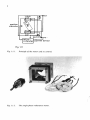
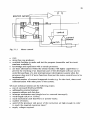
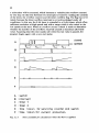
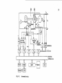
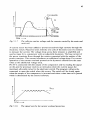
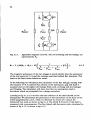
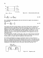
position
indicator
Fig. 1.1.1
Fig. /.J.l.
Principle of the motor and its control.
,
1
<I
.
•
v
.jo
:
,
•
.
~. ~
,,
?
,,.
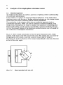
Fig. 1.1.2.
The single-ph ase reluctance motor.
3
1.
Qualitative description of the system
Compared with the A.C. series motor the single-phase reluctance motor has a
number of disadvantages, in particular a starting problem and complex control
electronics. In this section we give an account of the method used to eliminate the
drawbacks.
Fig. Lt.1 gives the configuration of a single-phase reluctance motor. The rotor
consists of a stack of laminated iron, mounted on a shaft. The current through
the coils is controlled by just one switch. If either one of the coils carries a
current in the situation shown, a torque is developed in the positive direction,
·
producing a motor action.
However when the rotor passes the vertical position, the torque becomes negative.
To reduce this negative torque, the switch is opened before the rotor attaîns the
vertical position. The switch is closed again when the rotor is near its horizontal
position and so on. Tuis switching action requires a rather sophisticated control
system.
Tuis motor unlike other motors requires no reversing of the current within one
revolution, because its torque is independent of the polarity of the current. Owing
to this characteristic just one switch suffices to control the motor.
lt will be clear that torque production is heavily dependent on the rotor positions
selected for closing or opening the switch; another important parameter in this
respect is the angular velocity, as will be discussed in chapter 2. A switching
action with satisfactory efficiency of the motor can be achieved by selecting
optimum rotor positions for every torque/speed combination.
Therefore proper control requires accurate information on the position of the
rotor at any given moment. This can be obtained from any suitable detector fitted
to the shaft. In order to keep the cost of production as low as possible we use a
very simple position sensor, which gives two pulses per revolution only. This
simple sensor, however, requires some sophistication in the electronic equipment
as will be discussed in chapter 3.
An important problem met in this type of motor is the start from standstill. For
this purpose two permanent magnets are fitted to the stator, which give the rotor
a favourable starting position under conditions we wil\ discuss in chapter 6.
Furthermore a special start procedure is implemented in the control unit.
Mainly for reasons of economy, as discussed in chapter 3, the control unit bas
been built around a microprocessor. For the processor we developed the software
to fulfil the following tasks:
• to determine the moment for opening and closing the switch;
• to start the motor;
• to protect the electronic switch against excessively high currents.
The software is designed to work with the simple sensor, providing two pulses per
revolution of the shaft.
4
2.
Analysis of the single-phase reluctance motor
2.1. Analytical approach
An analyticar description is usually a good way of getting a better understanding
of a particular phenomenon.
In this chapter we analyse the electromechanical behaviour of the single-phase
reluctance motor with the aim of finding relations between e.g. the average torque
of the motor, the motor constants and the control parameters.
The conclusion of this chapter will be that an analytica! approach leads to
complicated equations, which can only be solved by numerical methods, even
though many assumptions are made to simplify the equations. Considering their
limited applicability and the existing more flexible, numerical methods, this line
wil! not be pursued. Results of the analytica! method, however, are to be used for
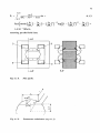
the verification of subsequent calculations.
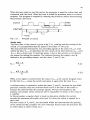
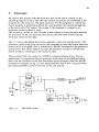
Fig. 2.1.1 shows a basic construction of the two-pole reluctance motor, which
consists of the stator yoke with coil and the rotor. This system acts as a motor by
energizing the coil in such a way that a positive mean value of torque is
developed, the positive direction of the torque being defined in the same direction
as that of the rotor angle.
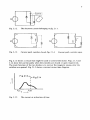
Fig. 2.1.l.
Motor provided with one coil.
5
Fig. 2.1.2.
The electronic circuit belonging to fig. 2. 1. l.
(
*'!
1
l
1
1
1
u
- -
..,
1
1
1
1
i
L_ __
-~-
(
~
u
r
l1~
1
~
_)
Fig. 2.1.3.
1
- - _j
\_
Current path, switches ciosed. Fig. 2. 1.4.
J
Current path. switches open .
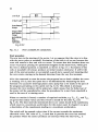
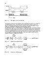
. Fig. 2.1.2 shows a circuit that might be used to control the motor. Figs. 2.1.3 and
2.1.4 show the current paths when the switches are closed or open respectively.
The main function of the two diodes is to recover the magnetic energy after the
switches are opened. Fig. 2.1.5 shows a current versus time diagram.
Fig.2.1.3;
1
.
Fig.2.1.4
1
1
ton
Fig. 2. 1.5.
t
-
toff
The current as a function of time.
6
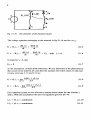
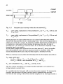
Fig. 2.1.6.
The motor provided with two coils. Definition of the angles a and p.
u
•
Fig. 2.1.7.
The circuit belonging to fig. 2.1.6.
- - -- -
f
u
u
1
1
•
-Fig. 2.1.8.
Switch closed.
-- -
r
1
\.__
Fig. 2.1.9.
'
1
Switch open.
~
i2
_)
•
7
An alternative way to control the current is presented by figs. 2.1.6 and 2.1.7. An
advantage of this solution is that only one switch and one diode are required, bul
here we have to provide a second coil on the stator. We call this additional coil
the catch coil and the other one the main coil. Tuis catch coil permits the
recovery of energy stored in the magnetic field after opening the switch.
The behaviour of both circuits (figs. 2.1.2 and 2.1.7) can be described w;th similar
analytica! equations. The following analysis will be based on figures 2.1 .6 and
2.1.7. The voltages and currents are defined in figures 2.1.8 and 2.1.9.
In
•
•
•
•
•
•
•
•
describing the second system we make the following assumptions:
the rotational speed of the rotor is constant and clockwise;
the currents carried by the main and the catch coil are periodic;
there are no eddy currents in the rotor and stator;
neither saturation nor hysteresis bas to be reckoned with in the rotor- and
stator iron;
the two coils wound on the stator have the same number of turns;
for the inductance of the coils a relation L(6) is assumed to be known;
the mutual inductance between the main and the catch coil is given by yL(fl);
the diode and the switch are ideal components.
The meaning of this last assumption is that the resistance of the component
equals zero in the conducting state and infinity in the blocking state.
As mentioned before, the control circuit determines when the switch is opened or
closed. In the following discussion it is assumed that the switch is closed when:
0
= -a - n/2 + kn
2.1.I
(see fig. 2.1 .6) and opened when:
0 = -f} + kn.
2.1.2
As we are treating the steady-state behaviour of the motor it is sufficient to
analyse the performance in the interval:
-n/2
a <9 <n/2 - a.
2.1.3
For further analysis we will require information about the initia! values of the
currents at the moment of the switching actions. At the moment t 00 , where 0
equals 7t/2-a, the switch is closed. Suppose that the current through the diode bas
a value
h(ton)
ho,
with
ho> 0.
2. I .4
8
R1 ,L(9}
u
•J. Ll9l
'----•
Fig. 2. 1.10.
The e/ements of the electrical circuit.
The voltage equations bel on ging to the network in fig. 2.1.10 are for t = t0 n:
_ R .
U - 111
+d{Li1) +
--
.
R 212
U=
dt
-
d(yLh)
dt
d(yL ii)
d(Lb)
dt
dt
---
2.1.5
+ ud.
with
b>
o.
2.1.6
1t ho Ids for i 2 > 0, that
2.1.7
on the assumption of ideal diode behaviour. We are interested in the phenomenon
that occurs in the interval AT, just after the moment the switch closes. In this case
we may write eqs. 2.1.5 and 2.1.6 as:
2.1.8
U
=
-
R .
.
212 - 11m
AT~()
A(Lh
+ yLi1)
!J.T
.
2.1.9
For a physical system we are allo wed to assume finite values for the .currents i 1
and i2• With this assumptlon the last two equations give for AT-0:
+ yL h = continuous
L h + yL ii = continuous.
L ii
2.1.10
2.1.11
9
Further we have:
2.1.12
with to-:. =ton+ .1t.
Combining eqs. 2.1.10 ... 2. 1.12 gives:
Y b(ton) = i1(t.in)
Îz(ton)
=
h(ttn)
+ Y b(t.in) -Y ho = i1(t.in) + Y h(ttn)
+ Y i1(t.in) -
Îio
Îz(t.in)
+ '( Îi(ttn).
2.1.13
2.1.14
When we multiply 2.1.14 by y, and subtract the result from 2.1.13 we get:
2.1.15
For y < > 0 it holds that:
2.1.16
Because of their bifilar winding, the two coils on the stator are assumed to be
fully coupled magnetically, so in our case we have:
2.1.17
y = l.
A verification of eq. 2.1.17 is given in section 2.3. Addition of eqs. 2.1.8 and 2.1.9
gives:
2.1.18
Together with eqs. 2.1.13 and 2.1.14 this yields:
2 U + Rzizo
R1 + R2
Î1(t:n)
= -----
iz(t.in)
=
-2U + Rsi20
2.1.19
2.1.20
The presence of the diode prevents the current i2 from going negative. lnspection
of eq. 2.1.20 shows that this occurs immediately after the moment the switch is
closed, provided that the following condition is satisfied:
.
2U
120<--.
R1
2.l.21
10
Eq. 2.1. t 3 gives for this case:
2.1.22
For the protection of the electronic equipment the control was made capable of
limiting the currents to a safe value. Tuis value was adjusted such that
.
0
2U
120<
Ri'
2.1.23
and consequently
2.1.24
When the switch opens at toir, following the same line of reasoning it can be
shown that
2.1.25
and
2.1.26
which is evident.
Now we know the behaviour of the currents at t =t 0 n and t = t0 wrespectively. This
knowledge will be used in the following treatment, where the currents will be
analysed for:
'
-7t/2
a <0 <
-P
and
-P <0 <11:/2 -
a.
2.1.27
The switch closes when:
9
= -7t/2 - a.
2.1.28
The initia! condition for the flux Jinkage is given by
~(-n/2
- a)
= L(-n/2
- a) ii(-n/2 - a).
2.1.29
We have the following equation for the circuit in fig. 2.1.10 when the switch is
closed:
2.1.30
11
Introduction of
(l)
= -de
dt
2.1.31
and
R1
2.1.32
dt'1 = -d0
roL
leads to
2.1.33
The solution of eq. 2.1.33 is
~(t1)
= exp(-T1)
j
Îl
~;
exp(t1') dt,'
+ Aexp(-T1).
2.1.34
0
Substitution of eq. 2.1.32 in to eq. 2. t .34 and use of the initial condition of
eq. 2. t .29 gives
L(0)it(0) =
~
e
exp(-î1)
j exp(1'1(0'))d0
1
+
2.1.35
-11/2-a
L(-n/2 - a) i1(-n/2 - a) exp(-1'1).
A good approximation for the inductance L(6), based on measurements, is
L(O)
= Lo +
L2 cos(20),
with L1 < Lo.
2. l.36
To reduce the complexity of the following expressions we introduce the
dimensionless variable
2.1.37
and the dimensionless parameters
R1
roLo
r1= - -
2.1.38
12
Lz
Lo
g= -
2.1.39
a 1(8) = (1 _ r1g2)' 12 arctan
{(l-g)112
tan(8) }.
1+
8
2.1.40
Now eq. 2.1.32 can be written in another form:
9
t,(9)
=
r, /
-n/2-a
t1(8) = 01(8)
1
1 + g cos <20 ,> da'
2.1.41
01(-n/2 - a).
2.1.42
Substitution of eq. 2.1.36 into eq. 2. t.35 leads to
. (0)
Ji
= r1exp(-01(8))
1
+ g cos(29)
j
9
'
exp\Ot
(81))d8'
+
2.1.43
-n/2-a
l - g eos(2a) .
1 + g cos(20) Ji(-n/2 - a)exp(-t1(8)).
Equation 2.1.43 applies for:
-n/2 - a
<8 <-P.
2.1.44
The same procedure can be followed to obtain the formula for the current i2•
Introduction of
ii(O) = R2 h(9)
2.1.45
u
2.1.46
a2(6)
=
(1
r 2g ) arctan {
2 112
(
1 - g ) 112 tan(&) }
t+g
2.1.47
2.1.48
leads to
13
r2exp(-a2{0))
1 + g cos(2e)
h(0) =
Jaexp(a2(0 ,)) d0 ,+ exp(-î 2(0)) *
2.1.49
-P
-P
J
r1exp(-01(-Jl))
{ 1 + g cos(20)
ex (01(0'))d0'
p
+
-1t/2-a
1 - g cos(2a) . (-1t/l
11
1 + g cos(20)
where the assumptions are made that
hC-P + A)
j1(-P - A)
with
2.1.50
A-+ 0
and
P < 0 < 1t/2 -
2.1.51
a.
As we are dealing with the steady-state behaviour of the motor we can write
M1t/2 - a
j1(1t/2 - a
A)
+ A) =
h(-1t/2 - a - A)
A-+O.
2.1.52
-P
exp(o1(0'))d0' -
2.1.53
with
Combination of equations 2.1.43, 2.1.49 and 2.1.52 leads to
î2(-1t/2 - ex))
j
-n/2-a
n/2-a
r2exp(-02(-1t/2
a))
j
exp(a2(0 1))d0 1 }
•
-P
[{l
gcos(2a)) Il
exp(-•1(-Jl)
•2(1t/2 - a)))] 1
With eqs. 2.1.43, 2. 1.49 and 2.1.53 the currents are given for
h(-1t/2 - a) > 0.
2.1.54
14
lf j 2(-x/2-a) equals zero, eqs. 2.1.43 and 2. 1.49 become by subsdtution of
j 2(-x/2-a) = 0:
8
i1(9)
= r1exp(-a1(9))
l + g cos(29)
J
exp(o11ll'\)d0'
1
2~1.s5
\V
-'lt/2-u
and
-P
jz(9) = {r1 exp(-o,(-P) - T2(9))
J exp(o (9')) d9' 1
2.1.56
-'ltf2-a
8
r2exp(-02(9))
J
exp(a2(9'))d9'}/u
+ gcos(29)1
-Il
Whether eq. 2.1.54 is fulfilled or not depends largely on the values of a and ~· To
express this condition in an analytica! form we use the following line of
reasoning:
lf i2(6) equats zero for 0=-7t/2-a then i2 can already reach zero for 6=6;., with
-P < 9z < n/2 -
2.l.57
a.
Then eq. 2.1.56 gives
-P
J
r1exp(-01(-P) - Ti(9z))
exp(o1(9'))d0 1 =
2.1.58
-x/2-a
r2exp(-02(9z))
j
&z
exp(o2(9'))d9'.
-P
The unknown value of ez can be determined by means of a numerical scanning
procedure.
In the foregoing we have found expressions for the currents through the motor
coils. The validity of the expressions 2.1.43, 2.1.49 and 2.1.53 depends on the
condition of eq. 2.1.54. If this is not valid, eqs. 2.1.55 and 2.1.56 have to be used
as long as j 2(6) > 0.
15
The mean torque
T of the motor is given by
2. l.59
Evaluation of the analytical equatioos
Our intention is to analyse the electromechanical behaviour of the motor in order
to show the inftuence of the control variables a and J) on the torque and the
efficiency of the motor.
To simplify the equations we have introduced many assumptions as mentioned at
the beginning of this section. Nevertheless the equations remain too complex to
be solved solely by analytica! means; in solving the equations a computer has to
be used.
With a computer, however, there are more straightforward ways of calculating
motor performance. Moreover a number of assumptions can then be discarded,
leading to a more realistic model. We propose the application of a completely
numerical method, which makes it possible to introduce a non-sinusoidal relation
between the inductance L and the rotor position Il and to allow for saturation in
the magnetic circuit.
The analytica! method of description developed in this section will be used as a
test of the following numerical approach.
2.2.
Numerical approach
To arrive at a more genera! method of describing the steady-state behaviour of
the single-phase reluctance motor we treat in this section a method based on the
time discretization of the differential equations.
As will be shown, the resulting formulas allow us to make calculations with a
non-sinusoidal relation between the inductance of the stator winding and the
rotor position. Some examples will be given to demonstrate the inftuence of the
control variables and conclusions will be drawn concerning an ideal reluctance
motor. In section 2.3 we also introduce magnetic saturation and for the
description we use formulas partly based on the expressions given in this section.
Fig. 2.2.1 shows the electrical diagram of the motor. In this section we assume
that magnetic saturation, hysteresis and eddy currents are absent. To make the
formulas valid for the time interval the switch is closed and open, we introduce
the variables a and Ra with the following characteristics:
-n/2 - a
+ kn
~
0<
~
+ kn-+ a = 1, Ra
corresponding to a closed switch and
R1
2.2.1
16
R1 • Ll9)
u
Fig. 2.2.1.
The electrical circuit. assuming that the two coils are fully
magnetically coupled.
-P + k1t ~ 0 < 7t/2 - a + kn -a =
-1, Ra= R2
2.2.2
corresponding to an open switch.
The equations belonging to the circuit, using the variables a and Ra, are:
.
aU =
T
R .
= i ·2
11
d(Li)
al+
2.2.3
--cït
dL
2.2.4
d0 .
In fact eq. 2.2.3 belongs to the circuit in fig. 2.1.3. But it also suits the circuit in
fig. 2.2.1 provided that the current i2 equals zero if the switch is closed and that
the current i 1 equals zero if the switch is open.
Further we have:
2.2.5
2.2.6
L = L(0)
0(t) = O(ti)
+j
t
co . dt = 0(t;)
+ co(t -
t;).
2.2.7
t;
The relation 2.2.6 bas to be specified in the program.
A Runge-Kutta procedure can be used to evaluate eq. 2.2.3 and 2.2.4 in
combination with eqs. 2.2.1 and 2.2.2, but numerical instability might then occur
17
if the differential equations are stiff (see ref. [4]). Since in the following st:ction the
motor will be described for the case where magnetic saturation is presen:, the
differential equations will indeed be stiff. Another problem connected with
available Runge-Kutta procedures is the required format of the input data. In
section 2.3 we represent the flux linked with the coils as a function of tht: current
and the rotor position by means of an array <l>(i"Oy), with a suitable nurr,ber x of
current values and rotor positions y. Available Runge-Kutta procedures are not
well suited to this kind of input, because they require an analytica! expression for
the linked flux.
To achieve uniformity in sections 2.2 and 2.3 we want to use one procedure to
find the solution of the differential equations in the more complicated situations
as wel!. In the following we write the differential equations as a set of difference
equations and solve these equations as a function of time.
To arrive at a set of difference equations we introduce:
2.2.8
I; = i(t;)
àl;
2.2.9
= Iï+1 -
I;
2.2.10
2.2.11
L{= dLI
d9
2.2.12
t=t;
2.2.13
9;
9(t;)
=
9;+1
=
2.2.14
9; +co àT.
2.2.15
We assume that the following condition holds:
t;
~
t
~ t;+1
2.2.16
Then we are allowed to use as an approximation:
L(t)
L1 + co(t
,
t;) . L ;
i
+ :i co
(t
t;)2 L"
àT
· ;·
2.2.17
2.2.18
18
Equation 2.2.17 is equivalent to
= L; + (0
L(0)
- 0;). L{
+t
~~+~ !i!~
.L{'.
2.2.19
To build up the difference equations we use the following algorithm:
~+I
f1(t)
= f2(t)-
AlT
j
4+1
f1(t') dt'
=
AlT
j
f2(t 1) dt'.
2.2.20
t;
Eq. 2.2.3 becomes
2.2.21
Substitution of eq. 2.2.17 and 2.2.18 into 2.2.21 leads to
a U = l;(Ra +co L! + lco L{')
+AI{;~
+ ro L;' + lw L{' + l Ra)·
2.2.22
The current AI; is the only unknown, which becomes after rearranging:
a U - l;(Ra + ro L{ + t ro L{')
Al;=---~~~~~~~--~~
L; +co L'; + ,ro
i
L"
AT
;
+
l
1
Ra .
2.2.23
The mean torque within the time interval t; •..t; + 1 is given by
2.2.24
or
2.2.25
To have a simpte accuracy check we introduce the following energy relations:
t;+1
wdiss,i
=
Wdiss.i-1
+
i
! i2Radt = I
t;
j=O
Ra(If + Alj.lj + iAif)AT
2.2.26
19
i
li+ !
W mech,i = W mech,i -
!
+
J
ffi
T dt
=
I
=
W;n,i-l
+
Tj AT
2.2.27
i
ti+ l
Win,i
CO
j=O
ti
J au
i(t') dt' =
ti
I
ai U(lj + j Alj)AT
2.2.28
j=O
2.2.29
The variable aj has the value of a at t = tj. _The calculation starts with t = t 0 and we
assume that the calculation ends at t t"" The energy balance at time tn is:
i Lo Ia + W;n,n =
W magn,n
+W
diss,n
+W
mech,n
+ AW
n•
2.2.30
The variable AWn represents the error due to the method used after n time steps.
To get an indication of the accuracy of the calculation we introduce
AWn
2.2.31
S=-Win,n
The value of this variable increases with increasing time step AT. The time steps
have to be shortened if the error is unacceptable.
With the expressions found we can analyse the inftuence of the control variables
a and 13 by means of computer calculations. Fig. 2.2.2 gives the flow chart of the
program.
Before the calculation starts for t = t0 we have to give the initia! conditions at
t = t0 , namely the rotor position and the current. We use as initia! rotor position
6 = -1t/2-a, where the switch is closed. It is assumed in the program that the
current in the catch coil might not be zero at the moment the switch doses.
Whether this is the case depends on the values of the control variables a and 13,
the speed and the motor constants.
If the inductance is given by eq. 2.1.36, then eq. 2.1.58 can be used to determine
whether the current i2 equals zero or not just before the moment the switch doses.
If not, eq. 2.1.53 gives us the right value of i2 at t = t 00 •
Knowing the initia! value of the current, it is sufficient to solve the equations for
the interval
-x/2 - a
~
e < x/2 -
a
to get the mean torque and the efficiency, whièh is defined as:
2.2.32
20
Procedure scanning a.~
Input: data motor and supply, áT. ro.
range a and ~. áa,áp
·
(eq. 2.2.26), Wmech.i (eq. 2.2.27),
W; 0 .1 (eq. 2.2.28)
e, + 1 < -a + it/2
WRITE 11. Î, a, ~
WRITE W0;".;, Wmech.i• W;n.i
Wdis..i
PLOT 11(a,~). î(a,p)
Procedure 10
2.1.58)
6,<n/2-a
N-;;--__
1" (eq. 2. 1.53) 1
Fig. 2.2.2.
..----Yes
l"=0
The flowchart of a numerical program that solves the equatians
belonging to the idealized reluctance motor.
21
2.2.33
where the index n means that at t = t 0 + 1 the rotor position 0 bas passed n/2-a. If
the inductance of the stator coil is not the same function as eq. 2.1.36 another
procedure should be followed. The current should be given an initial value and
the calculation of the current should be repeated until an acceptable small
difference exists between the calculated currents at -n/2-a + kn and
-1t/2-a + (k + 1)7t.
It is possible to verify the formulas develóped in this section by comparing the
results of the analytica! formulas described in section 2.1 with the results of the
computer procedure of this section. The analytica! expressions belonging to the
currents are eqs. 2.1.43 and 2.1.49; the mean torque is given by eq. 2.1.59. These
latter equations are solved by means of a numerical integration procedure
available for the computer used.
The input data used are:
R1
R2
4.275 Q
L(0)
0.102
4.275
Q
2.2.34
+ 0.0856 cos (20) H
2.2.35
=
u=
120
v
2.2.36
co
1571 rad/s.
2.2.37
Table 2.2.1 gives the results, which show fair agreement. The existing deviations
can be reduced by demanding a higher accuracy in the numerical programs.
a
~
torque
section 2.1
eff.
torque
section 2.2
eff.
(rad)
(rad)
(mNm)
(%)
(mNm)
(O/o)
0.0
0.0
0.0
0.3
0.3
0.3
0.6
0.6
0.6
0.0
0.3
0.6
1.36
8.83
8.35
70.26
20.71
21.42
38.87
137.4
37.33
61.4
94.8
95.9
34.7
92.7
93.8
6.5
49.9
90.8
1.36
8.83
8.35
70.10
20.71
21.42
38.66
137.4
37.33
61.3
94.8
95.9
34.6
92.7
93.8
6.4
49.9
90.8
Table 2.2.1
o.o
0.3
0.6
0.0
0.3
0.6
22
Fig. 2.2.3.
The behaviour of the relative error s of the energy balance as a
function of the time step L1 T.
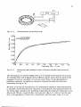
Fig. 2.2.3 shows the behaviour of eq. 2.2.31 as a function of the time step AT. We
consider the results presented in table 2.2.1 and fig. 2.2.3 to be an indication of
the correctness of the program. A proof that the method followed is suitable for
our purpose is given in section 2.3, where the method is extended to include
magnetic saturation and where the results of the new method are compared with
the results of measurements.
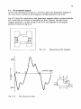
To show the inHuence of the control variables a and ~ we use the parameters of
the experimental motor as input for the program in fig. 2.2.2. We note that the
results are of limited value, because eddy currents, hysteresis and saturation in the
magnetic circuit are not included in this numerical procedure.
In the program the following constants and relations are used:
R1 = 4.35
L(0) = 0.102
U
ro
R2 = 4.35
Q
+ 0.0856 cos(20) H
220V
= 1571
a
2.2.38
2.2.39
2.2.40
rad/s
2.2.41
2.2.42
tJ.. T = 0.015/ro s
- n/2
Q
~
e < n/2 -
a.
2.2.43
23
l.0
0.5
Fig. 2.2.4a.
15
10
a(rud l___...o.s
Calculated torque at 15 000 r.p.m. The torque depends on the angles a
and fJ, which are defined in fig. 2.1.6.
to
t
/
/
1:1
0
~os
/
a!radl~
Fig. 2.2.4b.
/
/
10
15
Calculated efficiency. The dashed curve connects the sets of a and fJ
that give a maximum obtainable efficiency for every occurring value of
the torque.
24
"',-,,
..."----=----... ' ",45000
-g 0.6
-------:::.:--"
150001'
... - - - - - ,,,,,,,,
--- ----'5000 /r.p.m .
...:
CD.
T__...
0.4
0.2
0
~~~~~~~~~~~~~---
0
Fig. 2.2.5a.
0.2
0.4
0.6
0.8
1.0
a(rad )____....
1.2
Optimum sets of a and f3 for different speeds.
1.6
1.4
1.2
"*- 1.0
0
0
::: 0.8
F
E
g0.6
1-
0.4
0.2
0.2
0.4
0.6
0.8
1.0
Cloptirnurn -
Fig. 2.2.5b.
Efficiency and torque related to the curves in fig. 2.2.5a.
25
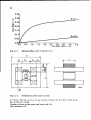
We have used fig. 2.2.3. to obtain a value for the time step AT that gives lln
acceptable error in the energy balance. We regard an energy balance errc r of Iess
than 0.1 o/o as acceptable, because the measuring error in the test rig will be larger.
Fig. 2.2.4 gives the curves with a constant torque (T) and a constant efficiency (Tl)
as a function of the control variables. The dashed curve connects the points
where a maximum efficiency is found for a certain value of the torque. In
fig. 2.2.Sa these curves are given for other velocities.
lt appears that steep gradients of both torque and efficiency are related to the
situation where i2 > 0 at t = t00 •
From these curves the following conclusiÓns are drawn:
• For every angular velocity ro and applied torque one set of values for a. and ~
gives a maximum efficiency.
• The value of~ is near 0.6 for these optimum combinations at the three selected
speeds.
• It is mainly the variable a that determines the value of the torque.
• If the value of the control variable a increases, a point is reached where the
current in the motor windings becomes continuous. In that situation the torque
assumes larger values, but efficiency decreases considerably (see fig.2.2.5b).
Apparently the continuous current is favourable for the torque production. At
the same time, however, the dissipation increases very fast. This is caused by
the presence of the current during the time the term dL/d6 is negative in
eq. 2.2.4. lts inftuence grows rapidly when a increases.
l.3. Analysis including saturation
In the preceding section the electromechanical behaviour of the motor was
described under the assumption of negligible saturation. In practice saturation
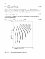
will be present, as shown in fig. 2.3.1, where the measured flux in our
experimental motors is given as a function of the rotor position and the current.
Each mark represents a measured flux value. These data were obtained in an
array cf>(i"6y) and will be used as input for the program that will be described in
this section. With this program the behaviour of the motor as a function of the
variables a and ~ can be obtained in a shorter time than by measuring the
behaviour in the test rig, even in our case where the measurements are automated.
The following assumptions are made:
• eddy currents and hysteresis are negligible.
• the electronic components are ideal.
• the angular velocity ro is constant.
• the main coil and catch coil on the stator are magnetically fully coupled, have
the same number of turns and their resistances remain constant.
26
1 -
0.2A
2 -0.4
3 -0.6
4 -OB
5 -10
6 1.4
7 ~ 2.0
6
9
10
11
12
-3.0
-40
50
60
7.0
2.0
Fig. 2.3. J.
The marks give the measured value of the flux related to a certain
current and rotor position.
•.....
u
2.4
main
catch
R1
eR2
12
Fig. 2.3.2.
The electrical circuit for the motor when magnetic saturation is
involved.
27
Figure 2.3.2 gives the following network equations:
U =
.
R111
()<IJ
+ ro -
ae
()<IJ di 1
ai1 -dt
+-
2.3.l
if the switch is closed, and
()<IJ dh
ae oh -dt
if the switch is open and i2 > 0.
- U
.
()<IJ
= R2 lz + ro -
+-
2.3.2
This includes the assumption that no current passes the catch coil if the switch is
closed (see the discussion in section 2.1).
The torque wil! be computed by way of the magnetic co-energy Wco (ref. [5]),
using the expression:
T = oWco
2.3.3
ae •
where the co-energy is defined as:
i
Wco =/<IJ
dil 9 =constant •
2.3.4
0
Inspection of the preceding equations shows that for every occurring combination
of the rotor position 6 and current i the values of é)<IJ/Oi, iJ4'/o0 and iJWc0 /ö0
should be available.
To get these function values use is made of a cubic spline interpolation (see
ref. [6D to interpolate the data of the flux measurements (see fig. 2.3.1) for both
the current and the rotor position in order to refine the grid 6,i. The refined grid is
given by:
0
0
~
1t/2,
.1.0 = 1t/60
2.3.5
and
Ai= 0.2.
2.3.6
In this grid the required functions are calculated at every nodal point and these
data are used in the program that solves the equations belonging to the motor.
For every combination of 6,i the above-mentioned functions are calculated by
means of a six-point interpolation of the function values at the surrounding nodal
points.
To analyse the behaviour of the torque and efficiency of the motor as a function
of the control variables a and~ with a numerical program the equations 2.3.1 and
2.3.2 have to be written in a time-discrete form, in accordance with the examples
given in the preceding sections.
28
First we reduce eqs. 2.3. t and 2.3.2 to
aU
.
= Ra 1 + ro
a~
a0
a~di
+ af dt
2.3.7
= i1
2.3.8
with
a = 1,
Ra
= R1
and
i
if the switch is closed and with
a = - 1, Ra = R2 and i
=
h
2.3.9
if it is open. The calculation of the current will start at t =ton• where the initia!
conditions are:
i
=0
2.3.10
0
=
-n/2 - a
2.3.11
a
=
1
2.3.12
ro = roo.
2.3.13
Using the algorithm of eq. 2.2.20 on eq. 2.3.7, we get
2.3.14
We assume that for the small interval
a = constant.
~T
we have
2.3.15
To obtain an approximated value of (J~/(}0 and (J~/öi, the value of the current
should be predicted for t > ti. We wil! use as extrapolation:
2.3.16
We define
Isugg
as:
2.3.17
The rotor position ai+ 1 is given by:
2.3.18
29
according to the assumption that the angular velocity is constant. On the basis of
the last equations the terms a<1>1ae and éJ<l>/ai will be:
2.3.19
2.3.20
Substitution into 2.3.14 leads to
2.3.21
The unknown current change AI; becomes:
a U - Ral; -
AI;= 2
a<1>
Ra+
i ro ( -a<1>
éJ0
(-a·1
1
0;,li
+
1
0i>Ii
a<I>
+ -a<1>
a0
1
)
0i + i.lsugg
~1
)/AT
vl
0; + 1,l,ugg
•
2.3.22
Under the constraint AT--0 we assume that it holds that:
2.3.23
The mean torque over the interval t;<t<t;+i becomes
2.3.24
The mean value of the torque and the efficiency over the interval t 0 •.. tn are given
respectively by
n-1
II-T
-n
i
j=O
and
2.3.25
30
n-1
11 =
!I
2.3.26
j=O
where ai means the value of a over the interval ti ... ti+ 1• The steady-state
behaviour can be described by repeating the calculation of equations 2.3.22 and
2.3.24 during the time that the rotor position is given by:
-n/2 - a
~0 ~n/2
2.3.27
- a.
If the current 1 is unequal to zero just for the moment t =t 0 "' the calculation
should be repeated until:
Il 9= -a+1t/2+k1t =Il 9= -a+1t/2+(k+l)1t +e,
2.3.28
1.5 . . . . . - - - - - - - - - - - - - - - - - - .
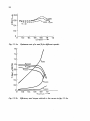
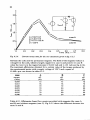
1.0
î
0.5
a(radl-- 0.5
Fig. 2.3.3.
The measured torque at 15 000 r.p.m.
1.0
31
where the varîable & represents an acceptable error. Here the steady-state mean
torque and efficiency should be calculated by using the results over the last
iteration, given by:
a
+ n/2 + kn
~
0
-a + 7t/2 + (k + 1)1t.
2.3.29
We are not interested in the case I > 0 at t t 0 m because the efficiency will be less
than we will accept for the applications we have mentîoned in the introduction.
The efficiency should be better than 60 O/o.
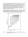
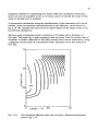
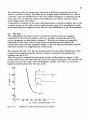
Fig. 2.3.3 and fig. 2.3.4 present the measured torque and efficiency of our
experimental motors as a function of the control variables a and ~· The
measurement equipment is described in chapter 4 and the dimensions of the
motor are given in chapter 6. We note that we have measured the torque by
"O
e
C!l.
0.5
Û'---'-~-'---'"~~~'---'-~....___.~_.___,
0
Fig. 2.3.4.
a(rad) -
0.5
The measured efficiency at 15 000 r.p.m.
1.0
32
means of the reaction tof~ue on the stator. The results of the program based on
the method described in this section are given in fig. 2.3.5 and fig. 2.3.6.
A fair agreement exists between figures 2.3.3 and 2.3.5, representing respectively
the measured and calculated torque. On the other hand, there is a great
discrepancy between the efficiency curves in figures 2.3.4 and 2.3.6. We note a
lower efficiency for all combinations of a and IJ and the shape of the curves is
different.
The following effects may contribute to this discrepancy:
• losses in the iron;
• non-ideal behaviour of the electronic components;
• increased resistance of the coils owing to temperature rise;
• increased resistance owing to high-frequency effects;
• faulty assumptions concerning the linkage of the catch and main coils.
1.5~-----------------.
g
c::i
1.0
î
0.5
O'---'-~..__.._~..__........~...____.~_.____....__.....
0
Fig. 2.3.5.
a (rad)--• 0.5
1.0
Calculated torque at 15 000 r.p.m. (including saturation). This figure
should be compared with fig. 2.3.3.
33
To check the last-mentioned possibility we have connected the coils in series and
in such a manner that the direction of the current of the main coil is oprosite to
the current carried by the catch coil. A full coupling should lead to a purely
resistive and frequency-independent character of the impedance of the two coils
connected in series. lt is only at frequencies higher than 5 kHz that a chrnge of
the impedance occurs greater than the measurement errors. The switching
frequency, which corresponds to the speed of 15 000 r.p.m., used for the
measurements, equals 500 Hz. Comparing this frequency with 5 kHz, we reject the
possibility of non-ideally coupled coils.
We assumed the resistance of the coils to_ be constant, so we neglected an increase
due to temperature rise and current displacement. The occurrence of the Jatter
effect is possible, hut cannot explain the strong increase of the losses, taking into
account the wire thickness (0.5 mm) and a basic frequency of 500 Hz.
1.0
î
0.5
o'---'-~-'---'-~-'-~"'----'-~-'---'----'----'
0
Fig. 2.3.6.
a(rad)- 0.5
1.0
Calculated efficiency at 15 000 r.p.m. (including saturation). Related
measurement given in fig. 2.3.4.
34
Introducing in the program the changing resistance of the coils due to the
temperature rise and the non-ideal behaviour of the electronic switch and the
diode leads to the results shown in figs. 2.3.7 and 2.3.8. Comparing figs. 2.3.6 and
2.3.8 we see a decrease of the efficiency of between t o/o and 3 O/o; there remains a
remarkable difference between the measured and the calculated efficiency
(figs. 2.3.4 and 2.3.8 respectively).
There remain the losses due to the eddy currents and the hysteresis in the
magnetic material used in the stator and rotor.
The nature of these losses is rather complicated. We point out that the flux does
not vary sinusoidally with time, that the distribution of the flux in the rotor and
the stator poles is not uniform and that the direction of the magnetic field with
respect to the rotor changes with time. So specifications given by the producer of
the lamination are not suitable to be used as data for a calculation. Numerical
1.5..-----------------.
.,.,
0
0
ei
1.0
l
"O
0
....
co.
0.5
a[radlFig. 2.3. 7.
0.5
1.0
The calculated torque after a correct ion for the temperature
dependence of the coil resistance and the losses in the power
electronics. Related measurement given in fig. 2.3.3.
35
programs suitable for calculating iron losses under the conditions mentioned
above are not yet available as far as we know, and it is beyond the scope of this
study to develop such a program.
Conventional calculations using the specifications of the lamination will not be
reliable. Such conventional calculations lead to the efficiency curves shown in
fig. 2.3.9. We consider the result to be an improvement of the shape of the curve,
but still not satisfactory.
We have used a Jamination with a resistivity of 70 µ!lcm and a thickness of
0.35 mm. The resistivity is high compared. with the usual value for silicon steel of
50 µilcm. A further reduction of the eddy current losses can be achieved by using
a magnetic circuit made of a lamination with a thickness of 0.1 mm instead of
0.35 mm.
1.5.---------------,
1.0
î
"O
....0
en.
95.0
0.5
O'---'--~'---'----J'--.....J----J~-'-----J~-'----'
0
Fig. 2.3.8.
a(rad)-
0.5
1.0
The calculated efficiency after the correction. Related measurement
given in fig. 2.3.4.
36
The improvement of the torque calculations obtained with the more complicated
model can be seen by comparing figs. 2.3.5 and 2.3.10. The Jatter figure shows the
results of the method described in section 2, where the following input is used:
2.3.30
R1 = 4.8 0,
+ 0.0901 cos(26) H
L(9) = 0.10S8
2.3.31
u=
120
v
2.3.32
ro
1S71 rad/s.
2.3.33
=
The maximum and minimum inductances in eq. 2.3.31 correspond to the
maximum and minimum flux of the experimental motor measured with a current
of 1 A.
1.5....-----------------.
1.0
!
v
"C
~
C!2.
0.
Q.___._--J,___._--J,___._--J,__--'-,.......~-'---'
0
Fig. 2.3.9.
a (rad, _ _ o.s
1.0
The ca/culated efficiency when the temperature rise of the coils, losses
in the power electronics, eddy current losses in the lamination and
hysteresis /osses in the lamination are included.
37
2.4 Conclusions
With a more sophisticated numerical model developed for describing the
electromechanical behaviour of the motor it is found that the calculated torque as
a function of the switch-on and switch-off time agrees wel! with the results of the
measurements.
The efficiency as a function of the same variables does not agree with the
measurements, most probably owing to eddy current and hysteresis losses in the
stator and rotor iron. An accurate calculation for the losses related to eddy
currents and hysteresis by analytica] means is difficult, because the ftux
distribution is not uniform and does not change sinusoidally in time and the
calculation has to include the rotation of the rotor in the pulsating field. As far as
we know, no numerical programs exist that can solve this problem and we
consider the development of such a program to be outside the scope of this study.
The consequence is that the efficiency of the motor should be obtained by
measurement.
1.5..--------------~
1.0
î
0.5
o~~__._.....___._~__._.....___.
0 a(radlFig. 2.3.10.
0.5
_
_.___.
1.0
This figure gives the torque when the linear model given in Ch. 2.2 is
used.
38
3.
Motor control
3.1. Selection of the control
In the preceding chapter we saw that the behaviour of the motor is to a large
extent determined by the va\ues of the control variables a and !}. For every speed
a certain combination of a and ~ can be found that gives a maximum efficiency
for the required torque at that speed. Now we have to decide on the control of
the motor and on the way in which to implement a mechanism that selects these
optimum va\ues.
Due to the characteristics of the motor an unusual procedure has to be applied to
start it. Tuis procedure too, which we discuss later on, has to be incorporated in
the control.
Another important aspect of the control is the protection of the power electronics
against too high currents.
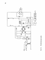
Signals that have to be available for the control are the ON/OFF signa! (given by
the user), the rotor position signa! and a signal indicating whether the current
exceeds the maximum value or not.
From the rotor position signàl the speed is obtained by measuring the time the
rotor needs to rotate over a certain artgle. Assuming a constant rotor speed this
angle might be e.g. 180 degrees. We choose this angle because a simpte and
relatively cheap sensor can be used to get'a pulse signal every 180 degrees. Tuis
gives the control the additional task of measuring the time between two successive
sensor signals to determine the speed.
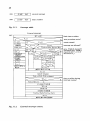
The current in the coils of the motor is determined by measuring the voltage drop
across two resistors connected in series with the two coils of the motor (see
fig. 3.1.1). The current in both coils has to be sensed, because due toa negative
value of ()(/)/()9 the current in the catch coil can risè above values allowed by the
switch. The switch should not be dosed when this occurs.
We propose the use of a microprocessor because it offers the following
advantages compared with other solutions such as discrete electronics, or analog
and digital integrated circuits:
• small size;
• low energy consumption (hence a small power supply);
• ftexibility during the experimental phase (no new wiring when changes are
necessary);
• complicated algorithms and features are easily introduced.
When the decision is made to use a processor, a member of a particular family of
processors bas to be chosen. Genera! considerations are:
39
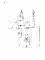
position sensor
con trol
Fig. 3.U.
•
•
•
•
•
•
Motor control.
cost;
more than one producer;
available facilities to make and test the program (assembler and in-circuit
emulator available?);
knowledge and experience with a certain processor;
are there alternatives (within the chosen family) with higher capabilities to
prevent the rewriting of an important part of the developed software and to
avoid the purchase of a new microprocessor development system when the
processor does not fit if more functions than just the motor control have to be
implemented?
required number of external integrated circuits (e.g. for the clock, timers and
communication with other parts of the system).
Of more technica! interest are the following topics:
• size of on-board RAM and ROM;
• addressable external memory;
• separate address and data bus;
• interrupt mechanism used (single level or vectored interrupt?);
• word length (4,8,16 or 32 bits);
• stack mechanism used (hardware or pointer-stack);
• number of timers;
• speed of the processor and power of the instruction set high enough in order
to reach the required execution times?
• supply voltages required.
40
To determine the power of;the instruction set important matters to be considered
are:
• the available ways of addressing a memory location (direct, indirect. relative
and indexed)?
• types of jumps;
• bit manipulation;
• ck operations;
• arithmetic instructions (double precision ?).
We selected the type 8048, a single-chip processor, because it meets all the general
questions mentioned above (see ref.[?]). When the type 8048 is compared with
other processors, however, it is seen to have a number of limitations (such as
speed, instruction set, stack and interrupt mechanism, memory size and number
of timers). If this processor is not suitable for applications of the motor that
require the implementation of other functions, a more powerful member of the
same family (e.g. the 8051) might be used.
3.2. Description of the control program
The information required for controlling the switch comprises the signals of the
position sensor and the current sensor. In this section we discuss how this
information is used, without going into the details of the program. At the end we
give a comparison between the time diagram for the processor used and the
diagram that would apply if the 8051 were used.
Input signals
The sensor for the rotor position gives a signal every .180 degrees. The processor
has to acknowledge this signa! immediately, because it contains the essential
information of the speed and the rotor position. From this information the
correct moment to open or close the electronic switch bas to be determined, for
which purpose we connect the signal with the interrupt input of the processor. To
record the time between two interrupts, which is related to the actual speed, we
use the 8-bit timer of the processor.
A signa) will be given by the current sensor when the current approaches the
maximum allowable value for the power electronics. Tuis signa! bas a high
priority, because to ignore it would lead to damage. Owing to the lack of a
second interrupt input this signa! bas to be fed to another input port or be mixed
with the signa! of the position sensor. In the Jatter case an additional signal bas to
be added to give the processor the information that the pending interrupt is
caused by the current detection. Because of the inductive character of the motor
the current cannot rise to unacceptable values within e.g. 20 µs, and this allows us
to connect the current detector with an input port of the processor. Tuis means
that the program should verify whether or not the current exceeds the maximum
value by a repetitive check of this port. In our program this is done every 25 µs.
41
When the user wants to start the motor, the processor is reset for a shor1 time and
connected with the clock. When the reset is ended the processor starts tt e con trol
program. The program is stopped by resetting the processor and by disconnecting
the processor and clock.
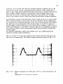
closed
switch
F""'===-~-"'==='-~--'/~.-~.~.~=·~·==~,.;====--opened
Îc,n+1ÎV'..n+ÎÎa,n+2Îb,n+2
interrupt 1----.,,.-----. .--------1..------.,.--Îi,n
Îi,n+l
-time
Fig. 3.2.1.
Principle of control.
Steady state
The basic idea of the control is given in fig. 3.2.1, starting with the closing of the
switch. It is assumed here that the speed is more than 11 720 r.p.m.
The measured time between the two preceding signals of the sensor (Ti,n) is used
within the time Tc,n+t to determine the new values of the time intervals Ta.n+ 2 and
Tb,n+ 2; this is done every 32 interrupt pulses. Later in this section we wil! discuss
the reason for taking this number. The relations between the angles a and ~'
defined in the preceding chapter, and the times T. and Tb are:
Ta=
Tt/2 - a
ro
3.2.1
Tb
n/2 + a - Il
ro
3.2.2
When a new signa! is received from the sensor (T w,n + 1) the control program waits
for the time Ta,n + 2, doses the switch and opens it again aft er the time Tb,n + 2•
A software timer is required to realize the times T. and Tb, because the type 8048
processor contains only one on-board timer and it is the task of this timer to
measure the time between the interrupt signals. We have developed for this
purpose a procedure whose execution time is adjustable by means of the value of
a variable.
In this procedure a regular check is made to determine whether the current
exceeds the maximum allowable value and, if it does, the switch is opened for a
short time.
The new values of T. and Tb are calculated within the time between the opening
of the switch and the reception of a new interrupt, because here the processor bas
no other tasks, as shown in fig. 3.2.2.
42
switch
interrupt
:Ta:
Îb
hardware
timer
executim
software 1--_.c:::::..i1----=::::::..."----c::.llf--timer
available
tor
calculations
Fig.3.2.2
Fig. 3.2.2.
Time available /or calculations.
Start procedure
We now turn to the starting of the motor. Let us suppose that the rotor is in line
with the stator poles at standstill. Excitation of the coils is of no use, because the
rotor will remain in line and will not rotate. To ensure that this situation does not
occur we propose placing two permanent magnets in the stator bore, which give
the rotor a defined position at standstill, as shown in fig. 3.1.1. Excitation of the
coils at standstill will always produce an initia! rotation clockwise. It will be the
task of the start procedure to accomplish a good start, a good start meaning that
the rotor starts rotating in the desired direction from the very first moment.
After the command to start the motor the program has to check whether the rotor
is rotating. If it is, then the speed has to be determined by measuring the time
between two successive interrupt pulses and a jump has to be made to the part of
the program pertaining to this speed (see fig. 3.2.3). Tuis check is necessary
because the rotor position will be unknown, which means that the behaviour of
the motor will be unpredictable when the procedure for a start from standstill is
used in the case of a rotating rotor.
When no rotation is found, a number of required variables, e.g. Tb,h Ta,2 and Tb,2,
are given their initia! values and the switch is closed for the time Tb,t (see
fig. 3.2.4), The time intervals mentioned above are values found from experiment,
which result in a maximum acceleration for the motor used. In chapter 6 we give
a description of the cxperiments leading to a maximum acceleration.
The switch wilt be opened a short time if the current exceeds the maximum
allowable value. The value of Tb,t is such that in practice the rotor has reached
the position where the sensor produces an interrupt when the interval Tb,t is
43
switch
closed
opened
interrupt
--•time
Fig. 3.2.3.
Rotating rotor at the start.
...
~============~:!..!:!.---=======----====----'===
opened
"
...
....
Îb,1
.....
Îa,2
interrupti-----------~,
Tb, 2
Îa,3
Tb,3
lflJ
100 ms.
---time
"-.>
Fig. 3.2.4.
Start /rom standstill.
passed. Once the interrupt is received, then the switch remains open for the time
Ta,2 and is closed again for the time Tb, 2•
The same time values are used again after the reception of the second interrupt
(Ta,3 =Ta,2 and Tb,3 Tb,2). After the third putse a "table look-up" procedure is
used to obtain new values for T. and Tb by means of the measured time between
the preceding interrupts. This will be repeated every five interrupt pulses until the
time interval is less than 2.56 ms (corresponding speed: 11 720 r.p.m.).
Supposing a very fast acceleration of the rotor in the case of a small load torque,
the interrupt wil! occur at an earlier moment than expected by the program, e.g.
in the time interval with a closed switch or within the time taken to calculate new
values of T. and Tb. We distinguish between two situations, namely when this
phenomenon occurs during the two start pulses and when it occurs in the time
afterwards.
Tb, 1:
open switch, replacement of the predefined T •. 2 by T' •. 2
T' b, 2 = T/2 (see fig. 3.2.5).
.28 ms and
44
closed
switch
opened
"
interrupt
---•~time
Fig. 3.2.5.
Tb. 2:
Tc, 1:
Reception of an interrupt within the time interval Tb.I·
open switch, replacement of the predefined Ta,3 by T' a,l =Ta.r1.28 ms and
T' b,3=T;f2.
open switch, replacement of the predefined Ta,2 by T' a,i=Ta.i-1.28 ms and
T' b,2 =T;f2.
During the start we cannot afford the loss of a pulse for the electronic switch,
because this increases the risk of a stillstanding rotor. The control program bas to
obtain new values of Ta and Tb by using the available information and this has to
be realized in a minimum of time, because the processor bas also the task of
guarding the Ta by means of a software timer.Soa calculation requiring a long
execution time is not possible.
As the speed is higher than expected, the new time interval Ta bas to be smaller
than the predefined value; the "same argument holds for the putse width. The
actions mentioned above are crude, but they require a minimum of time.
When an interrupt occurs within the following intervals the program proceeds to:
Tb,n: open switch and
for Ta,n>2.56 ms -Ta,n+l =T.,n-1.28 ms, Tb,n+I =T;/2
for Ta,n < 2.56 ms - new calculation for Ta,n+t and Tb,n+t
Tc,n: new calculation of Ta,n+l and Tb,n+t (see fig. 3.2.6).
The aim of these procedures is to ensure that the interrupt is not received at a
wrong moment a second time.
It is possible that the first pulse will not start the motor properly. To increase the
certainty that the motor will start, the first pulse is repeated when the time
between the first closing of the switch and the reception of an interrupt exceeds a
45
closed
switch
1---~~~======:!__~~_..;:==============-~opened
""-·
'---v-'
calculation
interrupt
,___. . . time
Fig. 3.2.6.
Reception of an inîerrupt within the time taken up by calculations.
maximum value. The start pulse is also given when the time between successive
interrupts exceeds that value. This check is built into the timer overflow routine,
which will be discussed later on in this section.
Speeding-up
Adaptation of T. and Tb, instead of after every five pulses, takes place every 32
pulses when the time between the two preceding interrupts is less than 2.56 ms.
The reason for this number of 32 pulses is that the microprocessor requi•es more
time than is available for the execution of the "table look-up" procedure at very
high speeds (e.g. 60 000 r. p.m.). When in this case the interrupt is received during
the determination of Ta and Tb, the switch remains open until a new interrupt is
received. Meanwhile the "table look-up" procedure is executed (see fig. 3.2.6.), so
one pulse in 32 might be absent.
Adaptation every 32 pulses gives rise to a delay time in the control loop, because
the actual values of T. and Tb belong to the speed measured between 2 and 33
interrupt pulses ago. An increase in delay time in a control loop leads to unstable
behaviour. The critica) value of the delay time depends on the transfer function
of the other components in the loop (see ref. [8]). We found by experiment that
the number of pulses should not be higher than 32 for our motor and control
program.
Timer
The on-board timer of the processor has the task of measuring the time that
elapses between two successive interrupts. The content of this timer is increased
automatically one step every n cycles of an oscillator connected with the
processor. The number of cycles is determined by some hardware components
connected with the processor. Starting and stopping of the timer are coupled with
the reception of an interrupt by means of some instructions in the program. An
overflow of this 8-bit timer sets the timer overflow flag and creates a timer
overflow interrupt. When this interrupt is acknowledged the ftag will be reset and
46
a subroutine will be executed, which increases a variable (the overflow counter)
by one step. So the time between two interrupts is found by reading the contents
of the timer, the overflow counter and the timer overflow ftag. The ftag bas to be
tested, because the timer overflow interrupt is not acknowledged under all
conditions. In this way the 8-bit timer is extended toa 16-bit timer, which offers
sufficient resolution at high speeds and with a range which is also suited to the
low speeds at the start. When an overflow occurs a check is made to determine
whether the number of the overflows received exceeds a maximum allowable
value. Assuming that the rotor stands still when this last value is passed, the
program begins again with a new start putse.
A
closed
i===:;::;;.==::====-;!=====:;:~=====;;==opened
Îb.n-1
B
c
D
E
-----~l--fli-----iu-
F
A : switch
B : interrupt
C : timer 1
D : timer 2
E : time taken for servicing counter and switch
F : time taken tor current protection
Fig. 3.2. 7.
Time available for calculations when the 8051 is applied.
47
8051 versus 8048
The more recent type 8051 processor has two 16-bit timers and two extemal
interrupt inputs; the use of this processor would result in a time diagram as
shown in fig. 3.2.7, which should be compared with the time diagram of the 8048
given in fig. 3.2.2. With the 8051 far more time remains available for det!rmining
T 3 and Tb, because the task of guarding the times T. and Tb is performed by the
second timer. The signa) of the current sensor might be connected with the second
interrupt input. In that case the time given by Il is claimed by the motor controL
Therefore when more functions have to be implemented (e.g. fora display or
other control functions) we advise the use of this processor. Since our aim up to
now is simply to control the motor, we use the 8048 processor, especially because
it costs about 70 % less to produce than the 8051.
3.3. Program
Tuis section gives a detailed description of the control program for the 8048.
To control the motor we need integer variables with a range from 0 to 65535,
which in terms of a microprocessor means 16-bit variables. The 8048 is an 8-bit
processor and to get 16-bit numbers we had to split the numbers into two parts,
e.g. T 3 (1), T.(2) and Tb(t), Tb(2). Each second term represents the most significant
part.
The following relations exist between the variables used in the preceding section
and the variables we will introduce now:
(Ta(l)
+ 256Ta(2)J * 5 µs
Ta
3.3.1
3.3.2
(T(l)
+ 256 T(2)} •
10 µs = T;.
3.3.3
Figs. 3.3.1 ... 3.3.6 present the flowchart of the program and fig. 3.3.7 gives the list
of symbols used. Two timers are used in the program, namely the hardware timer
of the microprocessor and a program loop (WAIT procedure). The time measured
by the hardware timer is given by:
{(timer)
+
256 (OVF
+ TF)J
• 10 µs,
3.3.4
where (timer) means the contents of the 8-bit timer, OVF the contents of the 8-bit
extension and TF the timer overflow flag (see section 3.2). lt is the divider, placed
between the clock and the timer input of the processor, that determines the time
10 µs (see chapter 5). The execution time of the WAIT procedure is:
(T(l)
+ 256 T(2)}
• 5 µs.
3.3.5
48
0003
JUMP
INT
external interrupt
0007
JUMP
TOF
timer overllow
Fig. 3.3.l.
Interrupt table.
External interrupt
INT
HT:=OF
~F1
F 1:=0
CLEAR
TIMER
OVF:=O
U:=I
RT:=2
ENABLE
TIMER
OVERFLOW
START
TIMER
limit timer overllow
1
N
;--__u=~y
1
X=Yvf
U:=I
Tb(2):=T(2), Th(l):=T(I)
>r~;Y;
r•f\
Y ~<2~
F 1:=1
~
~"(I~
T"(2):=
T.12)-1
start procedure active?
switch closed?
interrupt not allowed?
proc. TABLE aborted?/
execution proc. TABLE
required (set F3: = 1) or
decrement T"?
T"(I):= 1 T"( l):=T"( 1)-1
FJ:= 1 ~(I~
Fi:=O
1T"( I):= 1
F-':=I
(RETURN):=
REST
~I)~
F 1:=11
(RETURN):= LAB
F~:=I
STOP TIMER
T(2):=0VF. T( l):={timer)
y - - - - - - - T F = 1 - - - - - - - -N
T(2):= T(2)+ 1
1
CLEAR TIMER
TF:=O
OVF:=O
START TIMER
Tw(2):=T"(2). T.(l):=T.(I)
A:=I
RETURN RESTORE
Fig. 3.3.2.
External interrupt routine.
timer overllow during
interrupt routine?
49
We start with the external interrupt and the timer overflow interrupt. The
microprocessor is allowed to acknowledge an interrupt when this interrupt is
enabled and the instruction in progress does not belong to an interrupt service
routine. Once the interrupt is acknowledged, then the processor wil! stop the
program under execution, store on the stack the address of the next instruction
and make a call to location 0003 for an external interrupt and to 0007 for a timer
overflow interrupt (see fig. 3.3. 1). On these addresses the service routine:; start.
These routines have to be terminated with a RETURN RESTORE to indicate the
end of the service routine, which means that new interrupts might be
acknowledged and the interrupted program has to be continued.
For our application we need the facility that the program continues at a different
location when errors occur , e.g. when the external interrupt is received with a
closed switch. This is possible by changing the stored address on the stack, which
is indicated in the flow chart with: (RETURN):= .... (see ref. [9]).
Due to the interrupt mechanism of the processor used the putse length of the
interrupt should be Jonger than the time taken to execute the timer overflow
routine. The background of this requirement is that the processor does not
acknowledge an external interrupt received during the execution of the timer
overflow routine. Further the length should be shorter than the execution time of
the interrupt service routine. If it is not, the still pending interrupt signal will be
interpreted as a new interrupt when the execution of the interrupt service routine
is ended. This wilt lead to a wrong measurement of the speed of the motor.
Starting with the external interrupt routine INT (fig. 3.3.2), we meet the statement:
HT=OF. This means that when 15 timer overflows occur before a new interrupt is
received, the program has to be restarted at BEG in the Main program (see
fig. 3.3.3 and 3.3.4), because the velocity of the rotor is too low.
When the flag F 1 equals one, an external interrupt is received in the observation
time of 100 ms (see Main program), which means that the rotor is already moving
at the start of the program. In this case the timer is started from zero, and F 2: = 0
and F3 : = 1 indicate that the TABLE procedure has to be executed after the
reception of a new external interrupt to get the proper values for T 0 and Tb
belonging to the actual speed.
If the flag F 1 equals zero, then the state of the switch is tested by means of the
variable U. If the switch is open (U = 1) and the external interrupt is expected by
the program (F2 = 0), then the interrupted program will be continued after storage
of the value of the timer, the variable OVF and a test of the overflow flag TF.
Otherwise something was wrong and after the execution of RETURN RESTORE
the processor has to continue with the instructions, starting at LAB.
The following errors are possible:
• interrupt white the switch was closed (U = O);
• interrupt within the time T• (F2 = 1);
• interrupt during execution of the TABLE routine (F2 = 2).
50
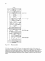
Timer overftow routine
OVF~=OVF+
TOF:
1
HT:=HT-1
time between interrupts
!""--...-=--------"y-> too long'!
U:=I
(RETURN):= BEG
DISABLE INTERRUPT
RETURN RESTORE
Fig. 3.3.3.
Timer overflow routine.
Main program
F1:=1
ENABLE INTERRUPT
Delay 100 ms
is the rotor
rotating?
DISABLE INTERRUPT
F1:=0. F,:=0, FJ:=O,
BEG:
reset flags
reset timer and
overflow
CLEAR TIMER
OVF:=O
HT:=OF, RT:=02
T"(l):=AO, Tw(2):=0A
T.(1):=50, T.(2):=04
Tb0):=50, Th(2):=04
ENABLE TIMER OVERFLOW
initialisation
START TIMER
close switch
U:=O
ENABLE INTERRUPT
(WAITTh)
REST:
A:=O
waiting for external
interrupt
A=O
1
~
F,~N
F.1:=0
F,:=2
(TABLE)
(WAITT.)
Tw(I ):=Th(I ), Tw(2):= Th(2)
execution of proc.
TABLE immediately'?
(WAITTh)
F,:=2
RT:=RT-1
~T=O
1 (TABLE)
F,:=0
Fig. 3.3.4.
Main program.
y
execution proc.
TABLE now '.:'
51
In the flowchart the corrections belonging to a certain error are given. The ftag F3
is set to one when a decrease of T. only is supposed not to be sufficient.
For the case F3 0 the elements of T w are given the correct values, which
determine the time between the interrupt and the closing of the switch. When
F3 =1, then Tw gets the final values in the TABLE procedure.
We draw attention to the statement A: 1 at the end of the external interrupt
routine, because this statement will be important when the instruction
(RETURN): LAB is not executed, which means that no error is found. This will
be treated later on.
The main program starts with a delay of 100 ms to see if the rotor is moving. If
no external interrupt (the signa! from the sensor) is received, the processor
continues with the initiation of some variables. RT = 02 means that after every
two interrupts the TABLE routine has to be executed to get new values for T. and
Tb· The length of the first pulse T w• the time between the first interrupt and the
second pulse (T.) and the length of the second putse (Tb) are set. Sequentially the
timer is started, the switch closed and the WAIT routine executed during the time
interval T w· In the latter routine the current overlaad protection is implemented,
which opens the switch when the current is too high. At the end of the WAIT
routine the switch is opened.
Returning to REST, the processor waits for an external interrupt by repeating a
short loop, which tests whether the variable A equals zero.
This loop is left for a short time after the reception of an external interrupt,
because the processor has to execute the external interrupt routine. In this routine
the value of A is changed to one, as mentioned before. Returning from the service
routine it is found that A = 1 and the loop is left.
The program waits for the time given by T• and sequentially the switch is closed
fora time given by the new values of Tb. Depending on the decremented value of
RT, the TABLE routine is executed before the processor continues the program
with the instructions starting at REST.
If the interrupt is received e.g. while the switch is closed, the program will be
continued at LAB also. In this case the ftag F3 equals one when correct values for
T. and Tb are not available and then the TABLE routine will be executed.
RT determines the number of external interrupts that has to be passed before a
new combination of Ta and Tb is calculated. The value of RT at the start was two.
This variable becomes five the first time the T ABLE routine is executed and
finally, when no timer overflow occurs, the value is changed to 32 ( &H20).
The task of the TABLE routine is to get proper values for Ta and Tb, belonging to
the actual values ofT(t) and T(2), which are related to the speed. Ifno timer
overflow has occurred (T(2) 0), two elements of the TAB array are selected. If
T(2) < > 0 then four values are selected and transferred to the elements of Ta and
Tb.
52
WAIT
coarse loop
X:=26
X<>O
Y:=3
Y<>O
current too high?
delay
fine loop
current too high?
U:=
U:=(U OR 1)
u..id
current too high?
U:=NOT(
RETURN
Fig. 33.5.
Wait procedure.
With the contents of the TAB array the torque-speed relation of the motor is
determined. Additional arrays have to be added to the program if an &pplication
requires several torque-speed relations. A particular torque-speed curve can be
selected in this casse by placing a certain value on an input port, which has to be
read by some additional instructions in the TABLE routine to select the correct
array.
TABLE
T 0(2):=0
A:=T(2) AND FC
T,(2):=0
T( l ): = TC 1)/2
X:=T(l) AND FE
T 0(l):=TAB(X)
T,(l):=TAB(X+ 1)
RT:=20
X:=80 X:=84
Ta(l):=TAB(X+2), T,(2):=TAB(X+3)
.RT:=05
RETURN
Fig. 3.3.6.
Table procedure.
54
3A. Condusions
The program described in this chapter performs the following tasks: it
determines the correct moment for opening and closing the electronic switch;
• it accomplishes a start from standstill and a good restart when the rotor is still
rotating;
• it protects the power electronics against too high currents.
The program developed allows the use of a sensor that gives just two pulses per
revolution, and if an application requires another torque versus speed curve than
the one implemented, it is only necessary to reprogram a table stored in the
processor.
As a concession to the program, we had tó add to the motor two permanent
magnets to give the rotor a well-known position at standstill to accomplish a
good start.
55
Flags:
F1 =0
F, 1
f,=O
F;=I
F2 =2
F 1 =1
Input:
Output:
Execute TABLE subroutine
Pending timer overflow
1
Current exceeds maximum value
l
U=O
X.Y.A
TAB
T
T"
T
T~
OYF
HT
RT
Fig. 3.3.7.
Interrupt allowed
Interrupt not allowed
Interrupt during execution of TABLE
subroutine
TF=I
U=l
Variables:
Condition
Start frorn standstill
Start with moving rotor
Switch closed
Switch opened
Temporary variables
Array, stored values of T" and T"
Array, time between interrupts
Arrav. used for WAIT subroutine
Array. switch-on time
Array, pulse width
Counter. number of timer overflow
Counter. guards OVF
Counter. number of interrupts to be passed
before adaptation of T" and Tt, in the
TABLE subroutine
Temporary variable
Symbols used in control program.
~
El"11<:1 +
U1n
multimeters
!.E.C. bus
~-...2J.:,___ _~L----LI----..U..---__l(;..-------....., doto-bus
L---.,..,.------...--------..,.r-----------~-___,oddress-bus
Apple
Plotter K:::I l.B.M.
Fig. 4.1.J.
Automated test rig.
Monitor
Disk
57
4.
Measuring equipment
In chapter 2 we used a method of calculation to describe the influence of the
control variables a and 13 on the torque and efficiency of a reluctance motor and
we compared this influence with the results of measurements.
This chapter deals with the equipment used.
The purpose of the measuring equipment is to measure the torque and efficiency
of a single-phase reluctance motor at a fixed speed, fixed supply voltage and at a
number of switch-on and switch-off angles. Changing these variables leads to a
large number of measurements and data. We have automated the whole test
procedure and the processing of the results to reduce the time required for the
measurements and thus bring forward the moment when figures become available
which describe the behaviour of the motor, and also to minimize the chance of
measurement errors.
Fig. 4.1.1 shows the complete measuring equipment, in which a microcomputer
accomplishes the tasks of genera! controller and administrator. We chose an
Apple Il computer, because the required hardware, e.g. digital-to-analog and
analog-to-digital converters and parallel input/output ports, were available for
this computer. All the measured data are stored on a magnetic disk and when a
measurement at a certain motor speed is finished the data are sent to another
computer (in our case an l.B.M. computer). On this computer the software
package G.P.C.P. (Genera! Purpose Contouring Program from Calcomp) is used
to make plots as given in fig. 2.3.3, which give a good impression of the behaviour
of the motor at the actual speed and supply voltage.
For the microcomputer we developed a program which controls the
measurements. When the required speed of the motor and the required
combinations of switch-on and switch-off angles are given, the program calculates
the required set-point for the speed control of the eddy current brake and
calculates the width of the pulses and the length of time between the signa! of the
rotor position sensor and the next pulse. We will call the latter time the triggering
moment. The triggering moment and the pulse width are transferred to a
simulator for the processor, which contains a program similar to the motor
control program described in chapter 3. A distinction has to be made between the
ways in which the pulse width and the triggering moment are obtained. Instead of
using a "table look-up" procedure, here we use the data placed on the input port
coupled with the microcomputer.
When the control program ·has accepted the new pulse width and triggering
moment, it sends a "ready" signa! to an electronic circuit to start the conversion
of the measured time between two sensor pulses (Ti), the measured pulse width
(Tb) and the measured triggering moment (T.) into analog signals. The
microcomputer reads these signals by means of three 10-bît AID converters.
58
The microcomputer gives the calculated set-point to the eddy current brake
control when the ready signal is sent. The brake causes the reluctance motor to
have the required speed by changing the braking torque. The set-point is adjusted
ifthe measured time T; does not agree within t %.
The torque of the motor is measured by means of the reaction torque on the
stator to eliminate the inftuence of the friction of the rotor hearings. We use a
torque measurement system made by Staiger-Mohilo. A low-pass filter is placed
between the torque meter and the related A/D converter to obtain the mean value
of the torque.
Two electronic multimeters are connected with the microcomputer by means of
an l.E.C. bus, a standardized form of comtnunication which enables the computer
to select one of the functions of the multimeter and to choose the right sensitivity.
The microcomputer stores the triggering moment and pulse width, the related
switch-on and switch-off angles, the measured time T;, the mean value of the
electromagnetic torque 'f, the supply voltage U;m the mean value of the supply
current 1;0 , the input power P, the effective current through the main coil lef!' and,
if required, the temperature 6 of the motor windings and the ambient
temperature.
Subsequently the whole range of required values of a and ~ is scanned. When all
measurements are completed, the data might be transferred to a printer to obtain
a list of the data or transferred to an l.B.M. computer via a modem to get a plot
of the torque and efficiency as a function of a and ~ for the speed and supply
voltage used.
Conclusions
The equipment described in this chapter measures automatically the steady-state
behaviour of the single-phase reluctance motor at a fixed speed and for a required
number of switch-on and switch-off angles.
The automated measurement method used reduces the chance of errors caused by
erroneous registration, and leads quite quickly to a graphical presentation that
gives a good impression of the behaviour of the motor. As we have seen in
chapter 2, there is a non-negligible difference between the measured and the
calculated efficiency of the motor. For this reason a test rig is required to
determine accurately the efficiency of the motor.
59
5.
Electronics
We deal in this chapter with the electronic part of the motor control. In the
preceding chapter we have seen that the control procedures are embodied in the
program for the processor. The input necessary for this program to control the
motor properly is information about the rotor position, the current through the
coils and an ON/OFF signa!. The output of the program is a signa) to an
electronic switch to open or close.
The electronic circuits we will consider in this chapter are the interfaces between
the processor on the one hand and the sensors, the ON/OFF switch and the
electronic switch on the other.
Fig. 5.1.1 shows the digital electronics required to start and stop the motor. The
electronic switch always has to receive the command to open the switch when the
motor has to be stopped. This is realized by a RESET command to the processor
during more than 50 ms. Within this time the processor reaches its initia! state,
which includes a command to the switch to open.
The command ON also results in a RESET command during 50 ms. For our
application it is important that the processor starts from its well-defined initia!
state with the execution of the first instruction of the program when the RESET
command is stopped. In fig. 5.1.2 the signals RESET and XTAL are given when
the command OFF or ON is received, as the case may be.
1----.---~RE SET
r1µF
on
Fig. 5.1.1.
ON/OFF circuit.
60
on/off
..------On
1---====-=-=-=---=--=-=-'-'J:!.._____ of f
>50ms
>50ms
time
Fig. 5.1.2.
The signals XTAL and RESET.
Information about the rotor position can be obtained by means, for example, of
an optical sensor and a two-slotted disc mounted on the shaft, as shown in
fig. 5.1.3. The given electronic circuitry produces the required number of two
pulses per revolution as discussed in the preceding chapter.
An altemative sensor is a Hall element in combination with a permanent magnet
(see fig. 5.1.4). Tuis sensor is less sensitive to dust and soiling and is cheaper, but
it involves accepting reduced accuracy in the position detection. For this reason
we use an optical sensor in our test rig. The use of a two-pole magnet entails that
on the negative and positive going edge of the sensor signal a pulse must be
created by means of single-shot circuits.
2rc
-----l-INT 8048
Fig. 5.1.3.
Circuit/or an optica! sensor.
Fig. 5.1.4.
Circuit/or a Hall element.
61
The output of the sensor electronics is connected with the interrupt input of the
processor. We have chosen a pulse width of 28 µs because the width has to be
Jonger than the execution time of the timer overflow routine and shorter than the
execution time of the interrupt service routine, as discussed in section 3.3.
8048
T,11
XTAL{
40
3
+5
39 ,__'"-'T"-1~
RESET
4
28 i-----::::t:::=--•
+5
26
+5
5
6
7
11
INT
Fig. 5.1.5.
1
2
20
ALE
t--9--~
The connections with the microprocessor.
The internal counter of the processor is used to measure the time between the
interrupt pulses. In fact the number of pulses received on pin Tt is counted (see
fig. 5.1.5) and by connecting this pin with a signa! of fixed frequency we ensure
that the contents of the counter will be related to the time elapsed between two
interrupts. The frequency is obtained by dividing the clock frequency by 60. On
the pin ALE is found the clock frequency divided by 15 and an external circuit
divides this signa! by 4, leading to the factor 60. Thus the counter is incremented
every t 0 µs with the clock frequency of 6 Mhz.
The output of the processor is the command to open or close the electronic
switch. One of the pins of the data bus (pin Pt t) is used as output for this signal.
The signa) is transmitted to the power electronics part of the system by means of
a pulse transformer, as shown in fig. 5. 1.6. The output of the transformer consists
of small pulses and positive feedback is used to ensure that these small signals
lead to an open or closed switch.
A snubber circuit is connected with the collector of the power transistor to
prevent damage from high transient voltages occurring during the opening of the
switch. The power supply for the motor comes from the rectified mains voltage
(220 V A.C.). Because of t~e characteristics of the circuit (see fig. 5.1.7), the power
transistor should be suitable for more than twice the rectified voltage.
62
63
tronsients
/-
1
\
1
'\.ecti fied
main
\ _voltage
\ 12
timeFig. 5.1. 7.
The cotlector-emitter voltage and the currents carried by the main and
catch coil.
A current sensor has been added to prevent excessively high currents through the
electronic switch. Placed in series with the two coils of the motor are two resistors
to measure the current. The voltage drop across these resistors is amplified and
used as input for a comparator with an adjustable hysteresis. The base current of
the power transistor flows through the resistor connected with the emitter of the
power transistor. This current introduces an additional voltage drop. For correct
operation of the current overload protection the hysteresis should have the same
value as this additional voltage drop.
Pin TO is connected with the output of the comparator and by reading the signa!
on this pin the processor receives an indication when the current passes the
maximum allowable value for the electronic switch. The program will give the
command to open the switch when this occurs. The switch will be closed again
when the output of the comparator is inverted and when a time interval is passed
which is determined by the control software.
Imox
î
"'
+
timeFig. 5.1.8.
The signa/ seen by the current overload protection.
64
65
From fig. 5. t .8 it will be clear that the chopper frequency depends only on the
time interval of the control, assuming that the hysteresis of the comparator is
equal to the voltage drop introduced by the base current. A smaller time interval
gives a higher chopper frequency and therefore leads to higher losses in the
electronic switch, due to the non-ideal behaviour of the switch, and to higher
losses in the snubber circuit. These losses limit the allowable chopper frequency.
An alternative circuit for the electronic switch is given in fig. 5.1.9, where a field
effect transistor (FET) is used to drive the power transistor. Fewer components
are required, but it depends especially on the cost of producing the FET whether
this solution is more economical. The circuits in figs. 5.1.6 and 5.1.9 require a
second supply to deliver the base current of the power transistor. With a view to
further development it is advisable to consider the use of a Darlington transistor
as a switch to achieve a more economical control circuit without a second low
voltage supply.
For domestic appliances a filter will probably have to be added bebind the
rectifier to prevent mains interference.
Figs. 5. t .10 and 5.1.11 give an example of the current carried by the main coil
and catch coil respectively. The switch voltage waveform is given by fig. 5.1.12.
Fig. 5.J .10.
Main coil current at 14 500 r.p. m" 120 V, a =0.62 rad and f3=1.02
rad.
Calibrations: 1.25 Aldiv, 0.5 msldiv.
66
Fig. 5.1.11.
Catch coil cu"ent.
Calibrations: 0.5 A/div, 0.5 ms/div.
Fig. 5.1.12. Switch voltage waveform.
Calibrations: 100 V/div, 0.5 ms/div.
67
Conclusions
The electronics necessary to control the motor are, besides the microprocessor:
• the electronic switch;
• a circuit for the position sensor;
• a circuit for the current sensor;
• an ON/OFF circuit for the processor.
A 5 V supply is used for the digital electronics and it depends on the electronic
switch used whether a second low voltage supply is required.
o.s
to
ts
2.0
2.s
3.o
3.s
Current (A) -
4.o
4.s
Measuredjlux at 8=0 and 8=1t/2.
Fig. 6.1.1.
b
AA'
A'
Fig. 6.1.2.
Dimensions of the motor in mm.
b= 70, b1 = 18.1, be= 15, b,= 11, h"= JO, he= JO, h5 = 13, h= 70, 1=29.5, d=8,
R, = 15.00, R, = 14.90.
Number of turns of the main and catch coil: 314.
Wire diameter: 0.5.
69
6.
Design aspects
In this chapter we will discuss a number of aspects related to the design and the
control of a single-phase reluctance motor. We will not deal here with the
optimization of the motor, because this depends to a great extent on the
application and on the weight factor of e.g. the costs. We consider that an
optimization, due to its complexity (see e.g. ref.[10]) is a separate study in itself.
The first section deals with the parameters governing the performance of the
motor, in particular the flux linked with the coils and the resistance of the coils.
In the second section we describe the influence of the permanent magnets. The
third section presents a procedure leading to the optimum Iength of the first and
the second pulse for the electronic switch and the optimum moment of triggering
the second putse, which largely determine the starting behaviour of the motor.
The last section deals with the supply voltage.
6.1. Flux and resistance
The performance of the single-phase reluctance motor is mainly determined by
the flux linked with the coils as a function of the angular position of the rotor
and the current. To implement the method given in section 2.3. we need the flux
for a limited number of rotor positions and current values. The required number
and the values depend on the shape of the function <l>(i,0).
Fig. 2.3.1 shows the flux linkage of one of our experimental motors. It is obvious
that a set of sinusoidal functions, depending on the rotor position, might be used
as a good approximation for the linked flux. Each function is related to a fixed
value of the current. We suggest the following function:
<l>(S) 1 i=constant
<l>o
+ <1> 2 cos(W),
6.1.1
in which the values of the unknown components <1> 0 and <1>2 depend on the value
of the current. In order to obtain these unknown components we need to know
the minimum and maximum value of the flux for every relevant current.
Fig. 6. t. t shows the linked flux at 6 =0 and 6 =n/2 as a function of the current
measured in the motor shown in fig. 6.1.2.
The maximum values are measured for the rotor position 6 = 0 and we remark
that the non-linearity of the relation between the flux and current is caused by the
characteristics of the iron parts of the motor, namely the stator and rotor
lamination and the shaft. lt is interesting to note the almost linear relation
between the flux and the current when the rotor stands at 0 = n/2. In order to
explain this we use the equivalent magnetic network for the motor given in
fig. 6.1.3. The flux linked with the two coils connected in series is given by:
70
1
1N·
2'
Po
1
Pgap
2
t
2
Pstotor
Protor
Pstotor
1
Pgap
...
t
Pa
Fig, 6.1.3.
èP
=
-1N·
2
[
Equivalent magnetic network. The coil overhang and slot leakage are
represented by Pa-
2.iN{èPm
+ èPa)
=
N2 (
2
/
l
+ -P rotor
- + P-stator
p gap
+
lPo)
i.
6.1.2
The magnetic permeance of the two airgaps is much smaller than the permeance
of the iron parts for 6 =O and the currents used (and related ftux densities). This
leads to the fairly linear behaviour noted.
In the following we will discuss the calculation of the flux linkage, starting with
the situation 6=0. A uniform flux density in the lamination, gap and shaft is
assumed and we will neglect the leakagefields (coil-overhang and slot leakage)
and fringing. The calculation will show that the two assumptions lead to
deviations which are acceptable for a design procedure.
Looking at fig. 6.1.2 it is obvious that the inftuence of the shaft should not be
disregarded. We determined the permeance of the lamination on the basis of the
initial magnetization curve, which we obtained by means of a ring of the
laminated iron used, as shown in fig. 6.1.4. The initia) B-H curve of the shaft is
measured with a permeameter. The flux linked with the motor coils, calculated by
means of fig. 6.1.3, is shown in fig. 6.1.5.
71
~lil
Plotter
t-
Fig. 6.1.4.
0.3
Î 0.30
Determination of the B-H curve.
calculated
--measured
~ 0.25
~ 0.20
u:::
0.15
0.10
0.05
O.OL----'-----'-----'---,___ _,___ __.__--'--...L.--.....1.
0.0
0.5
1.0
1.5
2.0
2.5
3.0
3.5
4.0
4.5
Current (A) Fig. 6.1.5.
Measured and calculated relatian between the flux and current at
8=0.
The discrepancy at currents higher than 2 A is caused by leaving out of account
the leakage fields and fringing, whose influence grows when the iron parts of the
magnetic circuit are saturated. At currents lower than 2 A the discrepancy is
probably caused by an unknown clearance between the shaft and the rotor
lamination (see fig. 6. 1.6).
We have to accept the introduction of a mechanical clearance when the material
is stamped, and furthermore the clearance is increased by the manual removal of
the sharp edges caused by the stamping. Supposing the respective clearances to be
40 µmand 100 µm, we get the flux curves given in fig. 6.1.7, where it can be seen
that a fair agreement is found for a calculation with the latter value. It is not
72
D
Fig. 6.1.6.
The clearance between the shaft
and the rotor lamination.
0.35
t
:0
~
0.25
0.20
x
-= 0.15
u.
0.10
0.5
1.0
1.5
2.0
25
10
15
40
Current (A) Fig. 6.1. 7.
The relation between the flux and the current at 8 = 0 aft er a
correctionfor the gap (seefig. 6.1.6).
possible to measure the clearance without damaging the rotor. With another rotor
we found a clearance up to 300 µm, so it is reasonable to take 100 µm as a
realistic value for the mechanical clearance introduced.
We consider this method of calculation to be satisfactory for a design procedure
because the discrepancy between the result of the measurement and the
calculation is less than S % for a current higher than 2 A.
For the situation 6=x/2 we take the permeance of the iron parts of the circuit to
be much higher than the permeance of the airgap. When we split the magnetic
field outside the iron parts into separate areas as shown in fig. 6.1.8 the permeance
for area 1, using the symbols in fig. 6.1.9, is given by:
73
bi/2
J
bi/2
µol
-(R-2_x..:...2-"-)1-12-_-b-tl2- dx
6.1.3
=
'
• ( bi )
bi {
( bi
2µ 0 1[ arcsm 2R, - iR, 1 -
2R,
)2} ·1/2 log {( l -
1.4 10- 7 Wb/A,
assuming parallel field lines.
1--A
3
3
AA'
Fig. 6. 1.8.
Flux paths.
--~1
1
f
1
Fig. 6.1.9.
Permeance calculation (eq. 6.1.3).
( bi
ZR,
)2)l/2 -
bi }]
ZR,
74
For area 2 we find in ref. (11}, p,. 134, eq. 11:
P2 = 0.52µ 0 1=0.19310- 1 Wb/A.
6.1.4
The slot leak:age in area 3 is given by (ref. [12D:
P3
= ( 3~c +
hs ;c he) µ 0 1 = 0.1565 l0- 7 Wb/A.
6.1.S
The inductance so far is given by:
6.1.6
The use of a two-dimensional field program such as MAGGY (see ref. [13]) leads
to 10.8 mH. We therefore consider eqs. 6.1.3 ... 6.1.5 satisfactory for our purpose.
The areas 4 and 5 are related to the third dimension, and the permeances for
these areas are as follows:
Area 4 (ref. [11], p. 132, eq. 8a and fig. 6.1.10):
J
bi/2
P4 =
(R;-
x~.1~~bi/l +
b1/2
- btf2
dx
=
0.64µob1arcsin
1
( 2~J = 0.09 J0-
7
Wb/A.
6.1. 7
Area 5 (ref. [11), p. 132, eq. 7):
Ps = 0.26 µ 0 b,
••
•
Fig. 6.1. JO.
= 0.059 10- 1
Wb/A.
..
t
Permeance calculation ( eq. 6. J. 7).
6.1.8
75
We were unable to find in the literature any analytica! method or tables for the
coil-overhang leakage in a configuration similar to our reluctance motor.
To show the importance of the coil-overhang leakage we note that
eqs. 6.1.3 ... 6. t. 7 give for the inductance
6.1.9
However a measurement gives 15.7 mH. Attempts to find methods giving an
upper and lower limit for the coil-overhang leakage required a large number of
assumptions in order to arrive at solvable analytica! equations. However the
assumptions tended to increase the unreliableness of the results (see also ref. (14))
and we conclude that a reliable determination of the inductance at 1t = 612 is only
possible by using a numerical field program such as e.g. PADDY (see ref. (15)),
which gave us an inductance of 15.6 mH.
Summarizing, we see that a simpte method can be used to obtain the flux for
0 = 0. However a three-dimensional numerical field calculation program has to be
used to obtain the flux at a= n/2. One calculation with such a program is
sufficient, because of the almost linear relation between the flux and current at
· 6=rc/2.
The results of these calculations can be used in the program described in
section 2.3 to determine the torque production of the motor in relation to the
speed, supply voltage and the value of the control variables a and Il
When a fin al design is obtained (e.g. optimized for an acceptable combination of
cost, mechanica! output power and dimensions) the flux as a function of the
current and rotor position can be verified by means of a three-dimensional field
calculation program, such as PADDY. We advise a three-dimensional program
because the neglected coil-overhang leakage and the fringing are essentially a
three-dimensional field problem, as mentioned in connection with the flux
determination at a= rc/2.
An equal flux density in all the iron parts at e 0 is used as the starting point for
designing the cross-section of the yoke, stator poles and rotor. Mechanica!
clearances and the available stamping tools introduce small deviations.
The flux in the rotor is assumed to be carried by the shaft as wel! (see fig. 6.1.7),
and of course one bas to take into consideration that this leads to losses due to
eddy currents in the solid iron shaft. We therefore consider the rotor given in
fig. 6.1.11 a better design, because less flux will be carried by the shaft, entailing
lower losses. The wider rotor also reduces the inftuence of the unknown
mechanica] clearance between the rotor lamination and the shaft.
As a compromise we have to accept an increase of the inductance at e=n/2. For
this rotor we measured an inductance of 17 mH, whereas the original rotor gave
15.7 mH, an increase of approximately 10 %. As a consequence the slope of the
flux line at e= n/2 in fig. 6.1.1 will also increase, which means a decrease of
76
0)
---~
.:::t"
Fig. 6.1.11 a. Dimensions of the wider rotor.
Fig. 6.1.11 b. The wider rotor.
77
approximately 2 % for the maximum obtainable mechanica! output power of the
motor.
Only experiments with different rotors wil! provide an answer to the question of
which cross-section of the rotor is optima! for a given cross-section of the shaft,
because the losses in the shaft cannot easily be calculated (see the discussion at
the end of section 2.3).
The airgap between the rotor and stator poles is t 00 µm. A decrease of the gap
will give a faster rise from i =0 for the <I> line at 6 = 0 in fig. 6.1.1. The area
between the two <I> lines increases, leading to a higher value of the maximum
obtainable mechanica! output power. However one should find an optimum
between the price to be paid for the decreased clearance and the increased output
power.
- We note that the inftuence of the decreased gap diminishes when saturation
occurs in the iron parts of the circuit, because then the magnetic resistance of the
iron will dominate.
In our design we have chosen the same width for the rotor and the stator poles
(18 mm). The result in our configuration is a fairly sinusoidal relation between the
flux and the rotor position at a fixed current. We note that this relation mainly
determines the torque production and the current carried by the coils as a
function of time.
In our motor the value of the tooth-width/tooth-pitch ratio is 0.38. In ref. [16) a
ratio of 0.35 ... 0.42 is given as optimum for the torque production. However
these values relate to the statie torque production in stepping motors, which have
a large number of teeth per pole. As far as we know, nothing has been reported in
the literature on the optimum relation between the flux linkage, rotor position
and current with respect to the torque production and efficiency of the reluctance
motor. A further study of this aspect is desirable.
In the reluctance motor we distinguish the bifilar-wound main and catch coils; the
coils have the same number of windings and their resistances are inversely
proportional to the copper cross-section. Choosing the same copper cross-section
for the wire of both coils is not the optimum if we consider the dissipation.
Assuming a fixed copper cross-section available for two coils, we have (see
fig. 6.1.12):
Acu
= Acu,m + Acu,c = a Acu + (1
- a) Acu·
6.1.10
For the sake of simplicity we have drawn two separate coils to represent the
bifilar-wound coils. Let the effective current for the main coil be Im and for the
catch coil Ic, then the dissipation is given by:
P(:)
_!L + I~
Acu,m
Acu,c
6.1.11
78
Ic
(1-cd
Nmain
Acu
Fig. 6. J.12.
= Ncotch
Cross-section of the coils.
or
P(:)
p
12
a Acu + (1 - ~) Acu
6.1.12
For a minimum total dissipation the ratio between the copper cross-sections is
then given by:
dP = O- Acu,c = ~.
da
Acu,m
6.1.13
Im
The result is the same current density in the wires of both coils. Looking at our
experimental motor with bifilar-wound main and catch coils, we observe the
effective current through the main coil to be much higher (note that the ratio also
depends on the control variables and a realistic value is 5). With eq. 6.1.13 an
optimum ratio of 5 is found between the cross-sections of both wires, and the
theoretica! decrease of the copper losses should be 31 % compared to the case
with equal wires.
For the production of bifilar-wound coils a ratio of 2 is the maximum allowable
value. A higher ratio will involve problems during the winding of the coils and
for this reason we cannot select the optimum cross-section ratio.
For further development we suggest experiments with two coils as shown in
fig. 6.1.13. These coils can be wound separately and the use of the optimum wire
size ratio is possible. One should pay attention here, however, to the Hux linkage
between the main and catch coils, since a decreased linkage will increase the
dissipation in the snubber circuit of the power electronics (see fig. 5.1.6).
Fig. 6.1.13.
Separate coils.
79
6.2 The permanent magnets
As has been discussed in section 3.1, we had to place two permanent magnets in
the stator bore to obtain an advantageous starting position for the rotor.
Fig. 6.2.1 gives the construction with permanent magnets which we found suitable
for a Ioad with low friction at standstill (less than 5 mNm). The field of the
magnets generates a torque acting on the rotor that depends on the angular
position as shown in fig. 6.2.2.
Fig. 6.2.1.
50.0
1
E
z
E
1-
-50.0
Fig. 6.2.2.
The measured torque.
Dimensîons of the magnets.
80
When a maximum speed is required after the first pulse given by the co1trol
circuitry the rotor position Oshould be slightly higher than 7t/2, becausc the
maximum amount of energy can then be transferred to the mechanical part when
the pulse ends at 6 =7t.
However a magnet configuration that leads to tbis starting position entails a high
sensitivity to friction torques, because the friction might cause a rotor position
slightly smaller than 7t/2, which leads to a wrong initia! rotation of the rotor.
Furthermore we note that the torque production of the motor is low when the
rotor position is near 7t/2, so the rotor will not rotate when the friction is too
high.
For this reason low friction is a necessary requirement with the the chosen
magnet configuration. In the design of th.e magnets the following aspects have to
be considered:
• the expected friction torque;
• the position at which the torque caused by the magnets gives a stable
equilibrium;
• the slope of the torque-versus-angular-position curve at the stable point.
We are still experimenting with a view to finding solutions that would allow a
load with a relatively high friction. This involves studying the influence of the
dimensions, position and the direction of the magnetization of the magnets.
-T1
C'
e ::O
Fig. 6.2.3.
A solution leading to a good starting position when the coulomb
friction is given between IJ or -T1 ( depending on the direct ion of
rotation).
A magnet configuration leading to the torque-angle relation given in fig. 6.2.3 is
one possibility. The rotor position at standstill will be in area A or B when the
coulomb friction torque is given between Tr and -T,. It should be in area B to
obtain the right initia! direction of rotation at the start. To ensure that the rotor is
at this position at the start, a limited current should be carried by the main coil.
The rotor will be attracted in line with the stator poles (6 1t or 0 = 0) and
subsequently the current should be switched off by the control. The torque caused
by the field of the magnets will force the rotor to the required area B. The starting
81
procedure described in chapter 3 can be used when the rotor has arrived in
area B. But, as mentioned before, this is still a subject of research.
Eddy current and hysteresis losses are introduced in the rotor and stator iron by
the field of the magnets when the rotor rotates. This might diminish the efficiency
of the motor compared with the motor without magnets. Furthermore since the
field of the magnets is linked with the coils (see fig. 6.2.4), this leads to a change
of the current through the coils as a function of time.
î
t
1.25
x
0
Fig. 6.2.4.
x
1t
e-
2tt
Linkage between the field of the magnets and the main coil.
X: closed switch (see fig. 6.2.6).
We have measured the torque and efficiency of the motor with the magnets for
the two cases shown in fig. 6.2.5; the difference between the two cases is a reverse
direction of the current in the coils. With an oscilloscope we measured the
currents as a function of time for a = 0.22 rad and 13 = 1.01 rad and a speed of
15 000 r.p.m. (see fig. 6.2.6). These curves show the influence of the flux linkage
Bifilar-wound
. - - - - - - - - - - - - - . m a i n and catch.--------------.
coils
case A
Fig. 6.2.5.
Reversal of current direction.
case
B
82
2.0
E
u
a. =0.22 rad
rad
rad/s
U =120V
p., =1. 01
w =1571
0.5
0.1
Fig. 6.2.6.
0.2
0.3
:~:.::::::::::::::::c=ase===A-.
caseB
0.4
0.5
0.6
0.7
time (ms l -
0.8
Current versus timefor the two situations given in fig. 6.2.5.
between the coils and the permanent magnets. The field of the magnets induces a
voltage E in the coils, which is largely negative in case A and positive in case B
when the rotor is in the region between 1t/2-0.22 rad and 1t-1.01 rad (see fig. 6.2.4).
The maximum efficiencies obtained for a certain value of the torque produced by
the experimental motor with a supply voltage of 120 V and a speed of
15 000 r.p.m. are shown in table 6.2.1.
case
A
B
torque
(Nm)
0.010
0.015
0.020
0.025
0.030
0.035
0.040
elf.
eff.
eff.
(%)
(%)
(%)
72
73
78
79
80
80
80
80
76
78
80
80
80
80
80
76
79
79
79
78
78
Table 6.2.1. Efficiencies found fora motor provided with magnets (the cases A
and B) and without magnets (case C). Fig. 6.2.5 shows the dilference between the
cases A and B.
83
We emphasize that the results were obtained at different combinations of the
control variables a and Jl The table shows slightly higher efficiencies for case B.
Column C gives the efficiencies for the case without magnets. Comparing case B
with case C we see that the values of the efficiency are almost equal at torque
values higher than 0.02 mNm.
A quantitative analysis of the observed phenomenon is hardly possible, due to the
complex nature of the eddy current and hysteresis losses. It is nevertheless worth
mentioning that the magnets do not lead to lower efficiencies in all circumstances.
6.3. The start
The single-phase reluctance motor is started by means of the two magnets
mentioned in the previous section, and by a number of pulses given by the
control program, as described in chapter 3. The first two pulses are especially
important for the start, and for this reason we describe in this section the
experiments that yield the optimum length of the first and second pulses and the
optimum moment for triggering the second putse.
We suppose that the rotor has the position given by the stable equilibrium in the
torque-versus-angular-position relation, which is created by the permanent
magnets (see fig. 6.2.2).
The start pulse is initiated by closing the switch, as discussed in chapter 3. The
switch opens when the time interval of the start putse has passed. The current will
be taken over by the catch coil and disappear quickly. Our aim is to reach the
highest possible speed after the start pulse.
32
Tv
1
28
U)
E 24
20
16
L__._.____.___._~-­
o
8 10 12 14 16 18
o
1
I
Îb :
Fig. 6.3.1.
start pulsQ !ms) -
Influence of the length of the start pulse.
-.;l
2800
A
~l/:-·
~~~?:
c.. 2400
~
.#;~:,,-·
"t:I
QI
QI
c.. 2000
111
·~/"'
2•
, ..........._
1200
0
Fig. 6.3.2.
/"
43 • ::;;.....--".
'
1600
2
.--·
/"
/
.,,,,,,... / '
4
6
8
10
.
1Sms Îa Îb
il r," ",
1
:
1
' 1
I sensor
~switch
start pulse
.
Îa: 1-6.6 ms
2-1.s ms
3-9.1 ms
4-10.5 ms
5-12.3 ms
6-13.3 ms
12
Tb: pulse width îms) -
lnjluence of the triggering moment and the length of the second pu/se.
85
A numerical description of the system might be used to determine the optimum
length of the start pulse. Calculations have shown a high sensitivity to the rotor
position at standstill (see Appendix). A prediction of the rotor position at
standstill is possible by means of the determination of the torque-versus-angularposition curve caused by the field of the magnets. The position at which the
torque becomes negative has to be considered as the position at standstill. A
measurement error of some degrees, however, will give a less appropriate length.
For this reason we advise practical experiments directed to the determination of
the optimum pulse length. In the following we give a procedure which we
consider most applicable.
We tested the proposed procedure on an experimental motor without load, a
supply voltage of 120 V and with the current overload protection adjusted to
3.2 A. Fig. 6.3.1 gives the relation between the length of the start pulse Tb and the
time T, between the beginning of the start pulse and the moment when the rotor
attains the in-line position.
A higher value for Tb than 17.7 ms leads to the situation where the switch is still
closed when the in-line position has been passed. In that case the torque reverses
and the rotor speed decreases. To prevent this unwanted situation we have
implemented a procedure in the control program that immediately cuts the pulse
when the rotor attains the in-line position (see chapter 3). For this reason we
stopped the measurements after Tb= 17 .7 ms. A length of 15 ms gives a value for
T, near the minimum and we wil! use this length for further experiments.
The load torque in certain applications is not fixed, for example when the motor
is used in a mixer. However the procedure mentioned above gave an optimum
start pulse only for one load.
The earlier-mentioned procedure in the control program offers a solution for this
problem. Let us suppose that we have followed the procedure to determine the
optimum start pulse in combination with the highest expected load, and that a
minimum for Tv is found at Tb=25 ms. The rotor will attain the in-line position
within the time of 25 ms when the load is small. The procedure mentioned above
cuts the start putse if the switch is still closed when the in-line position is reached.
Thus the length of the start pulse is automatically adapted to the load.
However the control program described in chapter 3 has to be changed to allow
the use of this mechanism.
For the second pulse we distinguish the triggering moment and the pulse width.
The optimum values depend on the angular velocity which the rotor bas reached.
So the following experiment bas to be carried out after settling the start pulse,
which we gave a value of 15 ms.
Fig. 6.3.2 shows the speed of the motor after the second pulse as a function of the
triggering moment and the length of the second pulse. The maximum value of the
pulse width is limited by the coincidence of the ending of the second pulse and
the reception of the sensor signa!. If we require the highest acceleration we prefer
the combination of Ta and Tb given by point A.
86
We conclude that simple experiments give the optimum values for the length of
the first two pulses and the moment of triggering the second one for a well-known
Ioad. Experiments are in progress to find an appropriate procedure for the first
pulses fitted for applications in which there is no well-defined load torque.
6.4.
Higher ratings with the prototype.
In chapter 3 we gave figures representing the characteristics of the experimental
motor (fig. 6.1.2) at a supply voltage of 120 V and a speed of 15 000 r.p.m.
Figs. 2.3.3 and 2.3.4 show an efficiency of 80 o/o ••• 81 o/o at a mean torque of
0.025 Nm (a=0.4 rad, j3=0.85 rad). In ~is case the mechanica! output power is
near 40 W. In the same figures an efficiency of 78 O/o is found at 0.05 Nm,
corresponding to 80 W (a=0.8rad,13=0.8 rad).
The temperature of the coils in the Jatter circumstances was appproximateJy 63° C
at an ambient temperature of 30° C. Considering the temperature rise higher
losses can be accepted, because the insuJation is capable of withstanding higher
temperatures. This fact allows experiments to see if higher ratings are possible.
To obtain an increased output power one could alter the control variables a and
13 in such a manner that the current carried by the coils becomes continuous as
discussed at the end of section 2.2. However a considerable decrease of the
efficiency has to be accepted in that case.
A better way is to increase the suppJy voltage. The circuit given in fig. 5.1.9 is
designed fora supply voltage up to 310 V (bebind the rectifier). We used this
suppJy voltage and altered the vaJues of the control variabJes a and 13 in our test
rig (see chapter 4) to determine the ratings.
The current is limited to a value of 4.2 A to prevent an excessive temperature rise
in the coil insulation. We measured a final temperature of more than 120°C at this
Jatter current vaJue under steady-state conditions. We found the ratings given in
tables 6.4.1 and 6.4.2 by altering the control variables a and J3. The power
delivered by the 5 V and 15 V supply and the Josses in the rectifier (see fig. 5.1.9)
were not taken into account for determining the efficiency with the test rig.
Our experimental motor was not provided with forced cooling. We expect that
the addition of forced cooling, allowing higher losses in the motor, would lead to
a higher obtainable output power.
We conclude that a mechanica! output power of more than 200 W is possible. It is
the temperature rise of the coil insulation that limits the allowable losses and,
related to these losses, the mechanica! output power.
87
Speed (r.p.m.)
Torque (Nm)
Efficiency (%)
Output power (W)
Temperature of the
coil-ends
10000
0.176
70
184
105
15 000
0.162
78
255
110
20000
0.110
82
230
80
Table 6.4.1. Measured maximum torque values, ambient temperature 35°C.
Speed (r.p.m.)
Torque (Nm)
Efficiency (%)
Output power (W)
Tem perature of the
coil-ends
10000
0.122
77.5
128
74
15 000
0.131
86
206
76
20000
0.077
85
161
54
Table 6.4.2. Measured maximum efficiency values, arnbient temperature 35°C.
88
7.
Conclusions
This study deals with the single-phase, electronically controlled reluctance motor.
The single-phase reluctance motor may be considered as one of the simplest
motors, because there are no windings of any type on the rotor, which consists
only of iron laminations. This simpte and robust rotor gives the motor a high
speed capability.
Furthermore there is no need to provide for a current reversal during one
revolution of the rotor. This characteristic allows the use of only one electronic
switch to control the motor, which considerably reduces the costs of the electronic
power circuitry.
.
In spite of its attractive points this single-phase motor bas two major drawbacks.
lts torque production is strong!y pulsating, which makes it unsuitable for
applications requiring a constant torque or speed, as for example in audio or
video equipment.
Another drawback is the starting problem. lt depends on the position of the rotor
at standstill whether the motor will start rotating in the required direction or in
the opposite direction. It is even possible that no rotation will occur. Provisions
have to be made to prevent this unwanted behaviour.
The starting problem is solved by mounting two permanent magnets in the stator
bore, which give the rotor a favourable starting position, and by an electronic
control system featuring an appropriate start procedure.
The torque production and the efficiency of the motor are mainly determined by
the rotor position reached at the moment the switch is closed and the position
when the switch is opened. For every rotor speed and applied torque a
combination of the switch-on and switch-off position can be found which gives
an optimum efficiency.
The electronic switch is controlled by means of a microprocessor, which obtains
the information required for the switching action by being supplied with the
signal from a rotor position sensor.
The costs of the sensor are reduced by an adaptation of the control program to a
sensor which gives only two pulses per revolution.
Within a wide range one or more torque versus speed relations can be selected by
programming the processor in an appropriate manner.
Experiments with our prototype proved that a mechanical output power of 200 W
can be obtained at 15 000 r.p.m. The efficiency under these circumstances was
78%.
Considering applications of the single-phase reluctance motor in domestic
appliances we have to compare our motor with the A.C. series motor. The stators
of both motors are fairly equivalent. However, the rotor of the series motor is
more complicated. Additional to the stack of laminated iron, as found in the
reluctance motor, the series motor contains a commutator, brushes and a number
89
of coils. The consequences of the additions are higher production costs and a
lower high-speed capability than we have found for the reluctance motor.
On the other hand the reluctance motor requires an electronic control system, the
most important parts of which are the microprocessor, the position sensor and
power electronic circuitry. The costs of the electronic control are mainly
determined by the power electronic circuitry. The use of a microprocessor makes
it possible to select one or more torque versus speed relations for the motor.
The solution of the starting problem with permanent magnets is suitable for
applications with a low friction and load at standstill. Further research is needed
to find a suitable solution for applications with a high friction and load at
standstill, as wel! as to optimize the single-phase reluctance motor for specific
applications.
90
References
(11 Lawrenson, P.J. and J.M. Stephenson, P.T. Blenkinsop, J. Corda, N._'l. Fulton
Variable-speed switched reluctance motors.
IEE Proc. B, Vol. 127(1980), p. 253-265.
121 Davis, R.M. and W.F. Ray, R.J. Blake
Inverter drive for switched reluctance motor: Circuits and
ratings.
IEE Proc. B, Vol. 128(1981), p. 126-136.
compon·~nt
131 Unnewehr, LE.
Series-commutated SCR controllers for variable-speed reluctance motor
drives.
In: PESC-73 Record: IEEE Power Electronics Specialists Conf., Pasadena,
Calif" 11-13 June 1973.
New York: IEEE, 1973. P. 180-191.
141 Dahlquist, G. and A. Björck
Numerical methods.
Englewood Cliffs, N.J.: Prentice-Hall, 1974.
Prentice-Hall series in automatic computation.
(51 Woodson, H.H. and J.R. Melcher
Electromechanical dynamics. Part 1: Discrete systems.
New York: Wiley, 1968.
(61 Mathematische Hilfsmittel des Ingenieurs. Teil 3.
Herausgegeben von R. Sauer und 1. Szabó.
Berlin: Springer, 1968. P. 265-277.
(7)
MCS-48 family of single chip microcomputers. User's manual.
Santa Clara, Calif.: Intel Corporation, 1978.
181 Marshall, J.E.
Control of time-delay systems.
Stevenage: Peter Peregrinus, 1979.
IEE control engineering series, Vol. 10.
(9)
Personality module PM 4321: User's manual.
Eindhoven (Netherlands): Philips (S&I).
Order No. 9499 620 01311. P. 5-13.
91
1101 Dijken, R.H.
Optimization of small AC series commutator motors.
Ph.D. Thesis. Eindhoven University of Technology, 1970.
1111 Roters, H.C.
Electromagnetic devices.
New York: Wiley, 1955.
1121 Vogt, K. et al.
Elektrische Maschinen: Berechnung rotierender elektrischer Maschinen.
Herausgegeben von G. Müller.
Berlin: VEB Verlag Technik, 1972. P. 275.
1131 Beer, A. de and S.J. Polak, A.J.H. Wachters, J.S. van Wely
MAGGY2 user manual.
Eindhoven (Netherlands): Philips (ISA), 1977.
1141 Corda, J. and J.M. Stephenson
An analytica) estimation of the minimum and maximum inductance of a
double-salient motor.
In: Proc. 3rd Int. Conf. on Stepping Motors and Systems, Leeds, 19-20 Sept.
1979. Ed. by A. Hughes.
Leeds: Department of Electrical and Electronic Engineering, University of
Leeds, 1979. P. 50-59.
1151 Beer, A. de and S.J. Polak, A.J.H. Wachters, J.S. van Wely
PADDY user manual.
Eindhoven (Netherlands): Philips (ISA), 1981.
Order No. 4322 270 07371.
1161 Harris, M.R. and A. Hughes, P.J. Lawrensoo
Statie torque production in saturated doubly-salient machines.
IEE Proc., Vol. 122(1975), p. 1121-1127.
92
List of symbols
a
variable, referring to an open switch. (a = t) or to a closed switch (a =-1)
be
width of the slots (m)
b,
width of the stator pole (m)
g
ratio
he
height of the coils (m)
hs
height of the slots (m)
i,
current carried by the main ooit (A)
i2
current carried by the catch coil (A)
i20
current carried by the catch coil just before the switch is closed (A)
ib
base current (A)
j1
normalized current carried by the main coil
j2
normalized current carried by the catch coil
~/Lo
length of rotor and siator (m)
r1
normalized resistance of the main coil
r2
normalized resistance of the catch coil
ton
moment at which the switch is closed (s)
tow
moment at which the switch is opened (s)
t
moment of time (s)
Acu
copper cross-section of the main and catch coils together (m2)
Aa..c
copper cross-section of the catch coil (m 2)
Acu.m
copper cross-section of the main coil (ml)
B
flux density (Wb/m2)
93
H
magnetic field strength (Alm)
Ii
current at t; (A)
120
current carried by the catch coil just before the switch is closed (A)
Ic
effective current carried by the catch coil (A)
Im
effective current carried by the main coil (A)
lsugg
extrapolated value of the current (A)
AI; t;
change of the current within a time interval starting with t; (A)
L
coefficient of self-inductance of the motor coils (H)
L°'L2
coefficients related to L (H)
L;'
dL/d6 at timet; (H/rad)
L;"
change of the dL/dO, defined by eq. 2.2.13 (H/rad)
N
number of tums of a coil
P."
permeance (Wb/ A)
P
power (W)
R1
resistance of the main coil (0)
R2
resistance of the catch coil (0)
Ra
represents R 1 and R2, depending on the value of a (0)
R.
radius of the stator bore (m)
T
torque (Nm)
T
average value of the torque (Nm)
AT
small time interval (s)
T.
time elapsed between the reception of an interrupt and the triggering
of the preceding pulse (s)
94
Tb
pulse width (s)
Te
time interval taken up by calculations (s)
T;
time interval between two interrupts (s)
coulomb friction torque (N m)
time interval (s)
time interval in which the processor waits for an interrupt (s)
supply voltage (V)
u
voltage drop over the diode (V)
amount of energy (Nm s)
w
angle related to the rotor position when the switch is closed (rad)
a
a
the ratio between the cross-sections of the main and catch coils in
section 6.2
13
angle related to the rotor position when the switch is opened (rad)
&
relative error in the energy balance, see eq. 2.2.31
&
discrepancy between two values of the current, see eq. 2.3.28 (A)
y
coefficient related to the linkage of the main and catch coils
fl
efficiency
e
rotor position (rad)
00
start position of the rotor (rad)
ez
rotor position where ii becomes zero (rad)
µo
constant (H/m)
95
angular velocity (rad/s)
infinitesimally small angle (rad)
flux linked with the coils of the motor (Wb)
coefficients related to <I> (Wb)
part of the flux (Wb)
leakage flux (Wb)
96
Appendix
In section 6.3 we discussed the optimum length of the first putse given by the
control circuitry at the start. To determine the optimum length we have i:hosen a
number of measurements with the experimental motor, because the length
depends to a great extent on the starting position of the rotor. Tuis appendix
gives the results of a simplified numerical description of the start to show the
influence of the starting position.
For the simplified model of the start we introduce a number of assumptions.
We suppose that the current carried by ~ain the coils arrives immediately after
the electronic switch is closed at the value given by the current overload
protection and it keeps this value until the rotor attains the in-line position. The
current is assumed to be zero in the main and catch coils when this position is
passed.
In practice a rise time of approximately 1 ms is found at a supply voltage of
t 20 V and a current overload protection adjusted to 3.2 A. The fall time found
under the same circumstances was approximately 2 ms. We neglect these times,
because they are small in comparison with the optimum length of approximately
15 ms which is found in section 6.3.
We use for the torque production of the motor with magnets (given in fig. 6.2.5,
case B) the measured torque-versus-angular-position curve at a current of 3.2 A
(see fig. A.t ).
Only a coulomb friction (Tr) is assumed and the inertia of the rotor J has the
value 1.48 to-s kg.m2.
To determine the angular position as a function of time we have to solve the
following equation:
0.5
l o e-0.5
Fig. A.l Torque production at 3.2 A.
97
2
d0
J dt 2
T
. ( d0)
+ Trs1gn
dt .
A.l
We solved this equation by numerical means and fig. A.2 gives the time interval
between the closing of the switch and the moment the rotor attains the in-line
position as a function of the starting position of the rotor (6 0). Furthermore this
figure gives the speed at the in-line position. Case A deals with a situation without
coulomb friction; in case B we introduced a friction of 0.02 Nm.
For both cases a minimum value of the elapsed time is found near 160°, but this
is not an interesting minimum because the final speed at 180° is low compared
with the obtainable speed at a start position in the range 90° ... 110°.
The consequence of the introduced coulomb friction, however, is no acceleration
if 90°<0<92°, because the generated torque is less than the coulomb friction of
0.02 Nm. One should use a starting position at which the generated torque is
higher than the friction torque when coulomb friction occurs.
Fig. A.2 shows that the time between the ignition of the pulse and the arrival at
the in-line position (and consequently the optimum length of the start putse)
depends to a great extent on the starting position when is this position is less than
l 00°. A small discrepancy between the assumed and the true starting position
leads to a considerably different value for the optimum length of the first pulse.
The high sensitivity of the optimum length to the starting position is caused by
the low value of the torque production near e= 90°.
With a view to the speed at the in-line position we conclude that a favourable
starting position is given by:
100°
A.2
< 0o < 110°.
00
î
u
00 $
Ul
E
<l>
E
time
10
O'--~~'--~~"'--~~"'--~~...&........J'--"o
90
110
130
150
170 180
90 (degrees)___.,.
Fig. A.2
98
Summary
Compared with the A.C. series motor the single-phase reluctance motor is
characterized by the simplicity of its construction. The rotor of the reluctance
motor consists only of a stack of iron laminations, whereas the rotor of the series
motor consists of a stack of laminated iron, a number of coils and a commutator.
Furthermore there is no need to provide for a current reversal during one
revolution of the rotor. This characteristic allows the use of only one eleetronic
power switch. In view of these attractive aspects this study was started to
investigate whether the single-phase reluctance motor could be considered as a
potential replacement of the A.C. series motor.
The reluctance motor does, however, have some drawbacks. Special attention bas
to be paid to the conditions leading to a good start, which implies that the rotor
must start rotating in the required direction with a high acceleration from the
very first moment of the start. Furthermore the single-phase reluctance motor bas
a strongly pulsating torque production and for this reason it is less suited for
applications that require a constant torque or speed as for example in video and
audio equipment.
It is shown that the motor can be described by means of analytica! equations
when a large number of assumptions are accepted. Due to the complexity of the
solution of the analytica) equations a computer bas to be used to obtain a
numerical result. A more realistic description of the motor is obtained when the
analytica! equations are replaced by a set of dilference equations, which can be
solved easily by a computer. The aim of the model is to predict the torque
production and efficiency of the motor. The results of calculations and
measurements show a fair agreement as far as the torque is concemed. A
considerable discrepancy, however, exists between the measured and calculated
efficiency, and we ascribe this fact to hysteresis and eddy current losses, which are
difficult to describe by analytica} or numerical methods.
The mean value of the torque and the efficiency of the motor depend critically on
the angular position of the rotor at the moments the switch is opened and closed.
For every applied torque and rotor speed a combination of the switch-on and
switch-otf position can be found which gives an optimum efficiency.
This study shows that a microprocessor is very well suited to act as motor
controller. With an adequate program the optimum switch-on and switch-off
positions in relation to the speed can be selected. Furthermore the torque-versusspeed relation of the motor can be altered by modifications of the program.
The motor controller requires information about the rotor position, and this is
provided by a simpte sensor which gives two pulses per revolution of the rotor.
We chose this simpte sensor for reasons of economy and adapted the program
accordingly.
r~
I .~
99
The combination of a suitable program and two permanent magnets in the stator
bore was chosen to solve the starting problem. This combination is well suited for
applications with a low friction and load torque at the start. Further research is
required to solve the starting problem in the case of a high friction or high load
torque.
Measurements on the prototype (which was not optimized) yielded a mechanica!
output power of approximately 200 W with an efficiency of 78 % at a speed of
15 000 r.p.m.
A number of aspects related to the optimization are discussed, but we consider
the optimization as a separate study in itself, due to the close relation between the
optimum design and the application.
Summarizing we conclude that the single-phase reluctance motor in combination
with the proposed control circuitry using a microprocessor should be considered
as a potential replacement of the A.C. series motor. Attractive aspects of this
motor are the simplicity of the motor and the required power electronics and
further the selectable torque-versus-speed relation, achieved by the use of a
microprocessor. However certain applications require careful attention to the
starting problem of this motor.
100
Samenvatting
Ten opzichte van de wisselstroom-serie-motor wordt de eenfase-reluctantie-motor
gekenmerkt door zijn grote eenvoud. De rotor van de reluctantie-motor bestaat
slechts uit een blikpakket. terwijl bij de serie-motor de rotor bestaat uit een
blikpakket, een aantal spoelen en een commutator.
Verder is de reluctantie-motor niet gevoelig voor de richting van de stroom in de
spoelen, zodat het niet noodzakelijk is de stroomrichting binnen een omwenteling
van de rotor om te keren. Door deze eigenschap is het mogelijk in de
motorsturing slechts een elektronische vermogensschakelaar te gebruiken.
Met het oog op deze aantrekkelijk aspecten werd deze studie gestart om te
onderzoeken of de eenfase-reluctantie-motor kon worden beschouwd als een
mogelijke vervanger van de wisselstroom-serie-motor.
Naast de voordelen van de onderzochte motor dienen de bijzondere eisen
genoemd te worden, waaraan voldaan moet zijn voor een goede start van de
motor, waarbij een goede start inhoudt, dat de motor vanuit stilstand direct en
met een hoge versnelling in de gewenste richting draait. Verder is het koppel van
de eenfase-reluctantie-motor sterk pulserend, waardoor deze motor minder
geschikt is voor toepassingen, die een constant koppel of toerental verlangen
(bijvoorbeeld audio- of video-apparatuur).
De beschrijving van de motor met behulp van een analytische model blijkt
mogelijk, indien een groot aantal vereenvoudigende veronderstellingen wordt
gedaan. De complexiteit van de langs analytische weg gevonden oplossing dwingt
ons echter om een rekenmachine te gebruiken om tot numerieke resultaten te
komen.
Een realistischer model van de motor kan verkregen worden door het analytisch
model te verlaten en te vervangen door een model, dat beschreven wordt door een
aantal differentie vergelijkingen, waarvan de oplossing op eenvoudige wijze
bepaald kan worden met een rekenmachine.
Het doel van het model is het koppel en rendement van een reluctantie-motor te
kunnen voorspellen. Een vergelijking van de resultaten van metingen en
berekeningen laat zien, dat het koppel goed berekend wordt met het numerieke
model. Een aanzienlijk verschil blijkt echter te bestaan tussen het berekende en
het gemeten rendement en wij schrijven dit toe aan wervelstroom- en
hysteresisverliezen, die zich door hun complexe aard moeilijk lenen voor een
numerieke of analytische beschrijving.
Het gemiddelde koppel en het rendement van de motor blijken sterk afhankelijk
te zijn van de positie van de rotor op de moment, dat de elektronische schakelaar
geopend of gesloten wordt. Voor ieder toegepast koppel is bij een zekere snelheid
een combinatie van ontsteekhoek en doofhoek te vinden, die een optimaal
rendement geeft.
101
Het onderzoek laat zien, dat een microprocessor zeer geschikt is om als centraal
orgaan te dienen in de besturing van de motor. Met de juiste programmatuur kan
de bovengenoemde afhankelijkheid van de motorsnelheid gerealiseerd worden.
Door het wijzigen van de programmatuur is de koppel-toeren-kromme van de
motor over een groot gebied beïnvloedbaar. Het programma, beschreven in dit
proefschrift, staat het gebruik toe van een eenvoudige en goedkope sensor, die
slechts twee pulsen per omwenteling van de rotor geeft.
De gekozen oplossing om een goede start te bereiken, bestaat uit een combinatie
van geschikte programmatuur en het plaatsen van twee magneten in de
statorboring. Deze oplossing blijkt te voldoen voor toepassingen, waarin een lage
waarde van het wrijvings- en belastingskoppel wordt gevonden bij de aanloop.
Verder onderzoek is nodig om een oplossing te vinden voor het aanloopprobleem,
indien de motor wordt gebruikt in een toepassing, waar een hoge waarde van het
wrijvings- en/ of belastingskoppel bij de aanloop optreedt.
Metingen aan het prototype laten zien dat een mechanisch vermogen van
ongeveer 200 Watt bereikbaar is bij een rendement van 78 O/o en 15000 toeren per
minuut. Wij merken op, dat het prototype niet geoptimaliseerd is. Een aantal
aspecten, samenhangend met een optimalisatie, wordt besproken, maar gezien de
nauwe samenhang tussen het optimale ontwerp en de toepassing, beschouwen wij
een optimalisatie als deel van een nieuw onderzoek.
Samenvattend mogen wij stellen, dat de eenfase-reluctantie-motor met de
voorgestelde besturing door een microprocessor beschouwd mag worden als een
mogelijke opvolger van de wisselstroom-serie-motor. Sterke punten zijn de
eenvoud van de motor en benodigde vermogenselektronica en verder de
mogelijkheid de koppel-toeren-kromme van de motor te veranderen door het
programma van de microprocessor aan te passen. Echter het gedrag van de
reluctantie-motor tijdens het aanlopen wordt sterk bepaald door de aard van de
belasting. Hieraan dient derhalve veel aandacht besteed te worden.
STELLINGEN
bij het proefschrift van J.C. Compter
4 mei 1984, Technische Hogeschool, Eindhoven
I
S.A. N asar beoordeelt een geïdealiseerde reluctantie motor aan de hand van
de verhouding tussen het mechanisch vermogen en het gewicht van de motor.
Zijn stelling. dat deze verhouding niet veel toeneemt door het verhogen van
de verhouding tussen de maximale en minimale zelfinductie, heeft geen
algemene geldigheid.
Nasar, S. A.
The goodness of a reluctance machine.
Proc. IEE, Vol. 118 (1971), p. 796.
II
Voor het bepalen van het dynamische gedrag van kleine elektrische motoren
kan met succes de techniek, die bekend staat als Laser-Doppler anemome. trie, toegepast worden in die gevallen, waarin meer conventionele meettechnieken falen.
Welling, W. A.
De Laser-Doppler-methode voor het meten van snelheden.
PT/Werktuigbouw, 37 (1982), No. 12, p. 72-75.
lil
Bij het ontwikkelen en testen van programmatuur, die bestemd is voor een
motorregeling met een microprocessor, is het verstandig om een simulator te
gebruiken voor de motor en zijn sturing.
IV
De nadruk, die gelegd wordt op het opgenomen vermogen van apparatuur,
die bestemd is voor huishoudelijk gebruik, snijdt de weg af naar alternatieve
oplossingen (bijv. een beter stofafscheidings-systeem in stofzuigers).
v
Elektrotechnische meetapparatuur (bijv. de oscilloscoop en de universeel
meter) kan in vele gevallen vervangen worden door een microcomputer met
adequate programmatuur en hardware. Het is derhalve verstandig de microcomputer als meetinstrument op te nemen in het praktische deel van de
ingenieurs-opleiding.
VI
Vriendelijkheid is kostbaar als dit betrekking heeft op programmatuur voor
computers en microprocessoren. Omdat niet-deskundige gebruikers met
deze programmatuur gaan werken, dient men toch aan de vriendelijkheid de
hoogste prioriteit te geven.
VII
De indeling van het QWERTY-toetsenbord is voor computergebruik voor
verbetering vatbaar.
VIII
Het gebruik van personal computers voor technisch en wetenschappelijk
rekenen dient afgewezen te worden, tenzij deze gekoppeld kunnen worden
met een netwerk.
IX
Het zal van grote betekenis zijn voor aankomende computergebruikers, als
er een onafhankelijke nederlandse organisatie komt, die de programma's van
de vele software-leveranciers test en kwalificeert.
Dowdney, D. L.
Software testing; Evaluation by independent groups gives buyers an
unbaised software standard.
Small Bus. Comput., Vol. 8 (1984), No. 1, p. 48-49.
x
Door het presenteren van hun telefoonnummers laten de omroepverenigingen zien dat men toch kan spreken over een verschil in identiteit.
4 mei 1984
J.C. Compter