Download Tutorial: Database Communication in LabVIEW

Telemark University College
Department of Electrical Engineering, Information Technology and Cybernetics
Database Communication
in LabVIEW
HANS-PETTER HALVORSEN, 2011.02.11
Faculty of Technology, Postboks 203, Kjølnes ring 56, N-3901 Porsgrunn, Norway. Tel: +47 35 57 50 00 Fax: +47 35 57 54 01
Preface
This document explains the basic concepts of a database system and how to communicate with a
database from LabVIEW.
You should have some basic knowledge about LabVIEW, e.g., the “An Introduction to LabVIEW”
training. This document is available for download at http://home.hit.no/~hansha/.
In addition to LabVIEW Professional Development System, you need to install the “LabVIEW
Database Connectivity Toolkit”.
For more information about LabVIEW and Databases, visit my Blog: http://home.hit.no/~hansha/
Some text in this document is based on text from www.wikipedia.org and “LabVIEW Database
Connectivity Toolkit User Manual”.
2
Table of Contents
Preface..................................................................................................................................................... 2
Table of Contents ....................................................................................................................................iii
1
2
3
Introduction to LabVIEW ................................................................................................................ 1
1.1
Dataflow programming ........................................................................................................... 1
1.2
Graphical programming........................................................................................................... 1
1.3
Benefits.................................................................................................................................... 2
Database Systems ........................................................................................................................... 3
2.1
RDBMS Components ............................................................................................................... 3
2.2
Data warehouse ...................................................................................................................... 4
2.3
Relational Database................................................................................................................. 4
2.4
Real-time databases ................................................................................................................ 4
2.5
Database Management Systems ............................................................................................. 5
2.6
MDAC....................................................................................................................................... 5
2.6.1
ODBC................................................................................................................................ 5
2.6.2
OLE DB ............................................................................................................................. 5
2.6.3
ADO (ActiveX Data Objects) ............................................................................................ 6
Relational Databases ...................................................................................................................... 7
3.1
Tables....................................................................................................................................... 7
3.2
Unique Keys and Primary Key.................................................................................................. 7
3.3
Foreign Key .............................................................................................................................. 9
3.4
Views ....................................................................................................................................... 9
3.5
Functions ............................................................................................................................... 10
3.6
Stored procedures ................................................................................................................. 10
iii
iv
Table of Contents
3.7
4
5
6
7
Triggers .................................................................................................................................. 11
Structured Query Language (SQL) ................................................................................................ 12
4.1
Queries .................................................................................................................................. 12
4.2
Data manipulation ................................................................................................................. 13
4.3
Data definition ....................................................................................................................... 14
4.4
Data types.............................................................................................................................. 14
4.4.1
Character strings............................................................................................................ 14
4.4.2
Bit strings ....................................................................................................................... 15
4.4.3
Numbers ........................................................................................................................ 15
4.4.4
Date and Time ............................................................................................................... 15
Database Modelling ...................................................................................................................... 16
5.1
ER Diagram ............................................................................................................................ 16
5.2
Microsoft Visio....................................................................................................................... 17
5.3
EXERCISES .............................................................................................................................. 18
Microsoft SQL Server .................................................................................................................... 20
6.1
Introduction ........................................................................................................................... 20
6.2
Requirements ........................................................................................................................ 20
6.3
SQL Server Express ................................................................................................................ 20
6.4
AdventureWorks ................................................................................................................... 21
6.5
SQL Server Management Studio ........................................................................................... 21
6.6
Create a new Database ......................................................................................................... 22
6.7
Backup/Restore ..................................................................................................................... 24
6.8
Example Database ................................................................................................................. 25
6.9
Exercises ................................................................................................................................ 27
Microsoft Office Access ................................................................................................................ 28
7.1
Introduction ........................................................................................................................... 28
Tutorial: Database Communication in LabVIEW
v
8
9
Table of Contents
7.2
Example Database ................................................................................................................. 28
7.3
Exercises ................................................................................................................................ 30
ODBC ............................................................................................................................................. 32
8.1
What is ODBC?....................................................................................................................... 32
8.2
Create an ODBC Connection in “ODBC Data Source Administrator” .................................... 32
8.3
Get data into Excel using your ODBC Connection ................................................................. 34
LabVIEW Database Connectivity Toolkit....................................................................................... 38
9.1
10
9.1.1
DSN ................................................................................................................................ 40
9.1.2
UDL ................................................................................................................................ 41
9.1.3
Connection String .......................................................................................................... 42
9.2
Reading Data from the Database .......................................................................................... 42
9.3
Writing Data to the Database ................................................................................................ 46
9.4
Creating and Dropping Tables ............................................................................................... 48
9.5
Using the Database Connectivity Toolkit Utility VIs .............................................................. 49
9.6
Performing Advanced Database Operations ......................................................................... 50
Creating and Using Tables ............................................................................................................ 52
10.1
11
Exercises ................................................................................................................................ 62
Creating and Using Triggers .......................................................................................................... 63
13.1
14
Exercises ................................................................................................................................ 59
Creating and using Stored Procedures ......................................................................................... 60
12.1
13
Exercises ................................................................................................................................ 55
Creating and Using Views ............................................................................................................. 56
11.1
12
Connect to the Database ....................................................................................................... 39
Exercises ................................................................................................................................ 66
Creating and using Functions ....................................................................................................... 67
14.1
Exercises ................................................................................................................................ 67
Tutorial: Database Communication in LabVIEW
vi
15
Table of Contents
SQL Toolkit .................................................................................................................................... 68
15.1
Installation ............................................................................................................................. 68
Tutorial: Database Communication in LabVIEW
1 Introduction to LabVIEW
LabVIEW (short for Laboratory Virtual Instrumentation Engineering Workbench) is a platform and
development environment for a visual programming language from National Instruments. The
graphical language is named "G". Originally released for the Apple Macintosh in 1986, LabVIEW is
commonly used for data acquisition, instrument control, and industrial automation on a variety of
platforms including Microsoft Windows, various flavors of UNIX, Linux, and Mac OS X. The latest
version of LabVIEW is version LabVIEW 2009, released in August 2009. Visit National Instruments at
www.ni.com.
The code files have the extension “.vi”, which is a abbreviation for “Virtual Instrument”. LabVIEW
offers lots of additional Add-Ons and Toolkits.
1.1 Dataflow programming
The programming language used in LabVIEW, also referred to as G, is a dataflow programming
language. Execution is determined by the structure of a graphical block diagram (the LV-source code)
on which the programmer connects different function-nodes by drawing wires. These wires
propagate variables and any node can execute as soon as all its input data become available. Since
this might be the case for multiple nodes simultaneously, G is inherently capable of parallel
execution. Multi-processing and multi-threading hardware is automatically exploited by the built-in
scheduler, which multiplexes multiple OS threads over the nodes ready for execution.
1.2 Graphical programming
LabVIEW ties the creation of user interfaces (called front panels) into the development cycle.
LabVIEW programs/subroutines are called virtual instruments (VIs). Each VI has three components: a
block diagram, a front panel, and a connector panel. The last is used to represent the VI in the block
diagrams of other, calling VIs. Controls and indicators on the front panel allow an operator to input
data into or extract data from a running virtual instrument. However, the front panel can also serve
as a programmatic interface. Thus a virtual instrument can either be run as a program, with the front
panel serving as a user interface, or, when dropped as a node onto the block diagram, the front panel
defines the inputs and outputs for the given node through the connector pane. This implies each VI
can be easily tested before being embedded as a subroutine into a larger program.
The graphical approach also allows non-programmers to build programs simply by dragging and
dropping virtual representations of lab equipment with which they are already familiar. The LabVIEW
1
2
Introduction to LabVIEW
programming environment, with the included examples and the documentation, makes it simple to
create small applications. This is a benefit on one side, but there is also a certain danger of
underestimating the expertise needed for good quality "G" programming. For complex algorithms or
large-scale code, it is important that the programmer possess an extensive knowledge of the special
LabVIEW syntax and the topology of its memory management. The most advanced LabVIEW
development systems offer the possibility of building stand-alone applications. Furthermore, it is
possible to create distributed applications, which communicate by a client/server scheme, and are
therefore easier to implement due to the inherently parallel nature of G-code.
1.3 Benefits
One benefit of LabVIEW over other development environments is the extensive support for accessing
instrumentation hardware. Drivers and abstraction layers for many different types of instruments
and buses are included or are available for inclusion. These present themselves as graphical nodes.
The abstraction layers offer standard software interfaces to communicate with hardware devices.
The provided driver interfaces save program development time. The sales pitch of National
Instruments is, therefore, that even people with limited coding experience can write programs and
deploy test solutions in a reduced time frame when compared to more conventional or competing
systems. A new hardware driver topology (DAQmxBase), which consists mainly of G-coded
components with only a few register calls through NI Measurement Hardware DDK (Driver
Development Kit) functions, provides platform independent hardware access to numerous data
acquisition and instrumentation devices. The DAQmxBase driver is available for LabVIEW on
Windows, Mac OS X and Linux platforms.
Tutorial: Database Communication in LabVIEW
2 Database Systems
A database is an integrated collection of logically related records or files consolidated into a common
pool that provides data for one or more multiple uses.
One way of classifying databases involves the type of content, for example: bibliographic, full-text,
numeric, and image. Other classification methods start from examining database models or database
architectures.
The data in a database is organized according to a database model. The relational model is the most
common.
A Database Management System (DBMS) consists of software that organizes the storage of data. A
DBMS controls the creation, maintenance, and use of the database storage structures of
organizations and of their end users. It allows organizations to place control of organization-wide
database development in the hands of Database Administrators (DBAs) and other specialists. In large
systems, a DBMS allows users and other software to store and retrieve data in a structured way.
Database management systems are usually categorized according to the database model that they
support, such as the network, relational or object model. The model tends to determine the query
languages that are available to access the database. One commonly used query language for the
relational database is SQL, although SQL syntax and function can vary from one DBMS to another. A
great deal of the internal engineering of a DBMS is independent of the data model, and is concerned
with managing factors such as performance, concurrency, integrity, and recovery from hardware
failures. In these areas there are large differences between products.
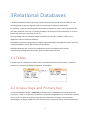
2.1 RDBMS Components
A Relational Database Management System (DBMS) consists of the following components:




Interface drivers - A user or application program initiates either schema modification or
content modification. These drivers are built on top of SQL. They provide methods to prepare
statements, execute statements, fetch results, etc. An important example is the ODBC driver.
SQL engine - This component interprets and executes the SQL query. It comprises three
major components (compiler, optimizer, and execution engine).
Transaction engine - Transactions are sequences of operations that read or write database
elements, which are grouped together.
Relational engine - Relational objects such as Table, Index, and Referential integrity
constraints are implemented in this component.
3
4
2

Storage engine - This component stores and retrieves data records. It also provides a
mechanism to store metadata and control information such as undo logs, redo logs, lock
tables, etc.
2.2 Data warehouse
A data warehouse stores data from current and previous years — data extracted from the various
operational databases of an organization. It becomes the central source of data that has been
screened, edited, standardized and integrated so that it can be used by managers and other end-user
professionals throughout an organization.
2.3 Relational Database
A relational database matches data using common characteristics found within the data set. The
resulting groups of data are organized and are much easier for people to understand.
For example, a data set containing all the real-estate transactions in a town can be grouped by the
year the transaction occurred; or it can be grouped by the sale price of the transaction; or it can be
grouped by the buyer's last name; and so on.
Such a grouping uses the relational model (a technical term for this is schema). Hence, such a
database is called a "relational database."
The software used to do this grouping is called a relational database management system. The term
"relational database" often refers to this type of software.
Relational databases are currently the predominant choice in storing financial records,
manufacturing and logistical information, personnel data and much more.
Strictly, a relational database is a collection of relations (frequently called tables).
2.4 Real-time databases
A real-time database is a processing system designed to handle workloads whose state may change
constantly. This differs from traditional databases containing persistent data, mostly unaffected by
time. For example, a stock market changes rapidly and dynamically. Real-time processing means that
a transaction is processed fast enough for the result to come back and be acted on right away.
Real-time databases are useful for accounting, banking, law, medical records, multi-media, process
control, reservation systems, and scientific data analysis. As computers increase in power and can
store more data, real-time databases become integrated into society and are employed in many
applications
Tutorial: Database Communication in LabVIEW
5
2
2.5 Database Management Systems
There are Database Management Systems (DBMS), such as:








Microsoft SQL Server
Oracle
Sybase
dBase
Microsoft Access
MySQL from Sun Microsystems (Oracle)
DB2 from IBM
etc.
This document will focus on Microsoft Access and Microsoft SQL Server.
2.6 MDAC
The Microsoft Data Access Components (MDAC) is the framework that makes it possible to connect
and communicate with the database. MDAC includes the following components:



ODBC (Open Database Connectivity)
OLE DB
ADO (ActiveX Data Objects)
MDAC also installs several data providers you can use to open a connection to a specific data source,
such as an MS Access database.
2.6.1
ODBC
Open Database Connectivity (ODBC) is a native interface that is accessed through a programming
language that can make calls into a native library. In MDAC this interface is defined as a DLL. A
separate module or driver is needed for each database that must be accessed.
2.6.2
OLE DB
OLE allows MDAC applications access to different types of data stores in a uniform manner.
Microsoft has used this technology to separate the application from the data store that it needs to
access. This was done because different applications need access to different types and sources of
data, and do not necessarily need to know how to access technology-specific functionality. The
technology is conceptually divided into consumers and providers. The consumers are the applications
Tutorial: Database Communication in LabVIEW
6
2
that need access to the data, and the provider is the software component that exposes an OLE DB
interface through the use of the Component Object Model (or COM).
2.6.3
ADO (ActiveX Data Objects)
ActiveX Data Objects (ADO) is a high level programming interface to OLE DB. It uses a hierarchical
object model to allow applications to programmatically create, retrieve, update and delete data from
sources supported by OLE DB. ADO consists of a series of hierarchical COM-based objects and
collections, an object that acts as a container of many other objects. A programmer can directly
access ADO objects to manipulate data, or can send an SQL query to the database via several ADO
mechanisms.
Tutorial: Database Communication in LabVIEW
3 Relational Databases
A relational database matches data using common characteristics found within the data set. The
resulting groups of data are organized and are much easier for people to understand.
For example, a data set containing all the real-estate transactions in a town can be grouped by the
year the transaction occurred; or it can be grouped by the sale price of the transaction; or it can be
grouped by the buyer's last name; and so on.
Such a grouping uses the relational model (a technical term for this is schema). Hence, such a
database is called a "relational database."
The software used to do this grouping is called a relational database management system. The term
"relational database" often refers to this type of software.
Relational databases are currently the predominant choice in storing financial records,
manufacturing and logistical information, personnel data and much more.
3.1 Tables
The basic units in a database are tables and the relationship between them. Strictly, a relational
database is a collection of relations (frequently called tables).
3.2 Unique Keys and Primary Key
In relational database design, a unique key or primary key is a candidate key to uniquely identify
each row in a table. A unique key or primary key comprises a single column or set of columns. No two
distinct rows in a table can have the same value (or combination of values) in those columns.
Depending on its design, a table may have arbitrarily many unique keys but at most one primary key.
7
8
Relational Databases
A unique key must uniquely identify all possible rows that exist in a table and not only the currently
existing rows. Examples of unique keys are Social Security numbers or ISBNs.
A primary key is a special case of unique keys. The major difference is that for unique keys the
implicit NOT NULL constraint is not automatically enforced, while for primary keys it is enforced.
Thus, the values in unique key columns may or may not be NULL. Another difference is that primary
keys must be defined using another syntax.
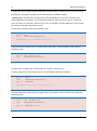
Primary keys are defined with the following syntax:
CREATE TABLE table_name (
id_col INT,
col2
CHARACTER VARYING(20),
...
CONSTRAINT tab_pk PRIMARY KEY(id_col),
...
)
If the primary key consists only of a single column, the column can be marked as such using the
following syntax:
CREATE TABLE table_name (
id_col INT PRIMARY KEY,
col2
CHARACTER VARYING(20),
...
)
The definition of unique keys is syntactically very similar to primary keys.
Likewise, unique keys can be defined as part of the CREATE TABLE SQL statement.
CREATE TABLE table_name (
id_col
INT,
col2
CHARACTER VARYING(20),
key_col SMALLINT,
...
CONSTRAINT key_unique UNIQUE(key_col),
...
)
Or if the unique key consists only of a single column, the column can be marked as such using the
following syntax:
CREATE TABLE table_name (
id_col INT PRIMARY KEY,
col2
CHARACTER VARYING(20),
...
key_col SMALLINT UNIQUE,
...
)
Tutorial: Database Communication in LabVIEW
9
Relational Databases
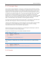
3.3 Foreign Key
In the context of relational databases, a foreign key is a referential constraint between two tables.
The foreign key identifies a column or a set of columns in one table that refers to a column or set of
columns in another table. The columns in the referencing table must be the primary key or other
candidate key in the referenced table. The values in one row of the referencing columns must occur
in a single row in the referenced table. Thus, a row in the referencing table cannot contain values
that don't exist in the referenced table. This way references can be made to link information
together and it is an essential part of database normalization. Multiple rows in the referencing table
may refer to the same row in the referenced table. Most of the time, it reflects the one (master
table, or referenced table) to many (child table, or referencing table) relationship.
The referencing and referenced table may be the same table, i.e. the foreign key refers back to the
same table. Such a foreign key is known as self-referencing or recursive foreign key.
A table may have multiple foreign keys, and each foreign key can have a different referenced table.
Each foreign key is enforced independently by the database system. Therefore, cascading
relationships between tables can be established using foreign keys.
Improper foreign key/primary key relationships or not enforcing those relationships are often the
source of many database and data modeling problems.
Foreign keys can be defined as part of the CREATE TABLE SQL statement.
CREATE TABLE table_name (
id
INTEGER PRIMARY KEY,
col2 CHARACTER VARYING(20),
col3 INTEGER,
...
CONSTRAINT col3_fk FOREIGN KEY(col3)
REFERENCES other_table(key_col),
... )
If the foreign key is a single column only, the column can be marked as such using the following
syntax:
CREATE TABLE table_name (
id
INTEGER PRIMARY KEY,
col2 CHARACTER VARYING(20),
col3 INTEGER REFERENCES other_table(column_name),
... )
3.4 Views
Tutorial: Database Communication in LabVIEW
10
Relational Databases
In database theory, a view consists of a stored query accessible as a virtual table composed of the
result set of a query. Unlike ordinary tables in a relational database, a view does not form part of the
physical schema: it is a dynamic, virtual table computed or collated from data in the database.
Changing the data in a table alters the data shown in subsequent invocations of the view.
Views can provide advantages over tables:






Views can represent a subset of the data contained in a table
Views can join and simplify multiple tables into a single virtual table
Views can act as aggregated tables, where the database engine aggregates data (sum,
average etc) and presents the calculated results as part of the data
Views can hide the complexity of data; for example a view could appear as Sales2000 or
Sales2001, transparently partitioning the actual underlying table
Views take very little space to store; the database contains only the definition of a view, not
a copy of all the data it presents
Views can limit the degree of exposure of a table or tables to the outer world
Syntax:
CREATE VIEW <ViewName>
AS
…
3.5 Functions
In SQL databases, a user-defined function provides a mechanism for extending the functionality of
the database server by adding a function that can be evaluated in SQL statements. The SQL standard
distinguishes between scalar and table functions. A scalar function returns only a single value (or
NULL), whereas a table function returns a (relational) table comprising zero or more rows, each row
with one or more columns.
User-defined functions in SQL are declared using the CREATE FUNCTION statement.
Syntax:
CREATE FUNCTION <FunctionName>
(@Parameter1 <datatype>,
@ Parameter2 <datatype>,
…)
RETURNS <datatype>
AS
…
3.6 Stored procedures
Tutorial: Database Communication in LabVIEW
11
Relational Databases
A stored procedure is executable code that is associated with, and generally stored in, the database.
Stored procedures usually collect and customize common operations, like inserting a tuple into a
relation, gathering statistical information about usage patterns, or encapsulating complex business
logic and calculations. Frequently they are used as an application programming interface (API) for
security or simplicity.
Stored procedures are not part of the relational database model, but all commercial
implementations include them.
Stored procedures are called or used with the following syntax:
CALL procedure(…)
or
EXECUTE procedure(…)
Stored procedures can return result sets, i.e. the results of a SELECT statement. Such result sets can
be processed using cursors by other stored procedures by associating a result set locator, or by
applications. Stored procedures may also contain declared variables for processing data and cursors
that allow it to loop through multiple rows in a table. The standard Structured Query Language
provides IF, WHILE, LOOP, REPEAT, CASE statements, and more. Stored procedures can receive
variables, return results or modify variables and return them, depending on how and where the
variable is declared.
3.7 Triggers
A database trigger is procedural code that is automatically executed in response to certain events on
a particular table or view in a database. The trigger is mostly used for keeping the integrity of the
information on the database. For example, when a new record (representing a new worker) added to
the employees table, new records should be created also in the tables of the taxes, vacations, and
salaries.
The syntax is as follows:
CREATE TRIGGER <TriggerName> ON <TableName>
FOR INSERT, UPDATE, DELETE
AS
…
Tutorial: Database Communication in LabVIEW
4 Structured Query
Language (SQL)
SQL (Structured Query Language) is a database computer language designed for managing data in
relational database management systems (RDBMS).
4.1 Queries
The most common operation in SQL is the query, which is performed with the declarative SELECT
statement. SELECT retrieves data from one or more tables, or expressions. Standard SELECT
statements have no persistent effects on the database.
Queries allow the user to describe desired data, leaving the database management system (DBMS)
responsible for planning, optimizing, and performing the physical operations necessary to produce
that result as it chooses.
A query includes a list of columns to be included in the final result immediately following the SELECT
keyword. An asterisk ("*") can also be used to specify that the query should return all columns of the
queried tables. SELECT is the most complex statement in SQL, with optional keywords and clauses
that include:





The FROM clause which indicates the table(s) from which data is to be retrieved. The FROM
clause can include optional JOIN subclauses to specify the rules for joining tables.
The WHERE clause includes a comparison predicate, which restricts the rows returned by the
query. The WHERE clause eliminates all rows from the result set for which the comparison
predicate does not evaluate to True.
The GROUP BY clause is used to project rows having common values into a smaller set of
rows. GROUP BY is often used in conjunction with SQL aggregation functions or to eliminate
duplicate rows from a result set. The WHERE clause is applied before the GROUP BY clause.
The HAVING clause includes a predicate used to filter rows resulting from the GROUP BY
clause. Because it acts on the results of the GROUP BY clause, aggregation functions can be
used in the HAVING clause predicate.
The ORDER BY clause identifies which columns are used to sort the resulting data, and in
which direction they should be sorted (options are ascending or descending). Without an
ORDER BY clause, the order of rows returned by an SQL query is undefined.
Example:
12
13
Structured Query Language (SQL)
The following is an example of a SELECT query that returns a list of expensive books. The query
retrieves all rows from the Book table in which the price column contains a value greater than
100.00. The result is sorted in ascending order by title. The asterisk (*) in the select list indicates that
all columns of the Book table should be included in the result set.
SELECT *
FROM Book
WHERE price > 100.00
ORDER BY title;
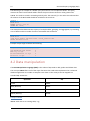
The example below demonstrates a query of multiple tables, grouping, and aggregation, by returning
a list of books and the number of authors associated with each book.
SELECT Book.title,count(*) AS Authors
FROM Book
JOIN Book_author ON Book.isbn = Book_author.isbn
GROUP BY Book.title
Example output might resemble the following:
Title
Authors
------------------------------SQL Examples and Guide
4
The Joy of SQL
1
An Introduction to SQL
2
Pitfalls of SQL
1
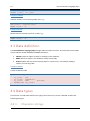
4.2 Data manipulation
The Data Manipulation Language (DML) is the subset of SQL used to add, update and delete data.
The acronym CRUD refers to all of the major functions that need to be implemented in a relational
database application to consider it complete. Each letter in the acronym can be mapped to a
standard SQL statement:
Operation
SQL
Create
INSERT
Read (Retrieve)
SELECT
Update
UPDATE
Delete (Destroy)
DELETE
Example: INSERT
INSERT adds rows to an existing table, e.g.,:
Tutorial: Database Communication in LabVIEW
14
Structured Query Language (SQL)
INSERT INTO My_table field1, field2, field3)
VALUES ('test', 'N', NULL)
Example: UPDATE
UPDATE modifies a set of existing table rows, e.g.,:
UPDATE My_table
SET field1 = 'updated value'
WHERE field2 = 'N'
Example: DELETE
DELETE removes existing rows from a table, e.g.,:
DELETE FROM My_table
WHERE field2 = 'N'
4.3 Data definition
The Data Definition Language (DDL) manages table and index structure. The most basic items of DDL
are the CREATE, ALTER, RENAME and DROP statements:



CREATE creates an object (a table, for example) in the database.
DROP deletes an object in the database, usually irretrievably.
ALTER modifies the structure an existing object in various ways—for example, adding a
column to an existing table.
Example: CREATE
Create a Database Table
CREATE TABLE My_table
(
my_field1
INT,
my_field2
VARCHAR(50),
my_field3
DATE
NOT NULL,
PRIMARY KEY (my_field1)
)
4.4 Data types
Each column in an SQL table declares the type(s) that column may contain. ANSI SQL includes the
following datatypes.
4.4.1
Character strings
Tutorial: Database Communication in LabVIEW
15
Structured Query Language (SQL)




CHARACTER(n) or CHAR(n) — fixed-width n-character string, padded with spaces as needed
CHARACTER VARYING(n) or VARCHAR(n) — variable-width string with a maximum size of n
characters
NATIONAL CHARACTER(n) or NCHAR(n) — fixed width string supporting an international
character set
NATIONAL CHARACTER VARYING(n) or NVARCHAR(n) — variable-width NCHAR string
4.4.2


BIT(n) — an array of n bits
BIT VARYING(n) — an array of up to n bits
4.4.3



Numbers
INTEGER and SMALLINT
FLOAT, REAL and DOUBLE PRECISION
NUMERIC(precision, scale) or DECIMAL(precision, scale)
4.4.4




Bit strings
Date and Time
DATE
TIME
TIMESTAMP
INTERVAL
Tutorial: Database Communication in LabVIEW
5 Database Modelling
5.1 ER Diagram
In software engineering, an Entity-Relationship Model (ERM) is an abstract and conceptual
representation of data. Entity-relationship modeling is a database modeling method, used to
produce a type of conceptual schema or semantic data model of a system, often a relational
database, and its requirements in a top-down fashion.
Diagrams created using this process are called entity-relationship diagrams, or ER diagrams or ERDs
for short.
There are many ER diagramming tools. Some of the proprietary ER diagramming tools are ERwin,
Enterprise Architect and Microsoft Visio.
Microsoft SQL Server has also a built-in tool for creating Database Diagrams.
16
17
Database Modelling
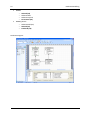
5.2 Microsoft Visio
Microsoft Visio is a diagramming program for creating different kinds of diagrams. Visio have a
template for creating Database Model Diagrams.
Tutorial: Database Communication in LabVIEW
18
Database Modelling
In the Database menu Visio offers lots of functionality regarding your database model.
“Reverse Engineering” is the opposite procedure, i.e., extraction of a database schema from an
existing database into a database model in Microsoft Visio.
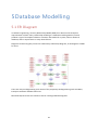
5.3 EXERCISES
Exercise: Database Diagram
Create the following tables in an ER Diagram using MS Visio.


CUSTOMER
o CustomerId (PK)
o FirstName
o LastName
o Address
o Phone
o PostCode
o PostAddress
PRODUCT
o ProductId (PK)
o ProductName
o ProductDescription
o Price
o ProductCode
Tutorial: Database Communication in LabVIEW
19
Database Modelling


ORDER
o OrderId (PK)
o OrderNumber
o OrderDescription
o CustomerId (FK)
ORDER_DETAIL
o OrderDetailId (PK)
o OrderId (FK)
o ProductId (FK)
Database Diagram:
Tutorial: Database Communication in LabVIEW
6 Microsoft SQL Server
6.1 Introduction
Microsoft SQL Server is a relational model database server produced by Microsoft. Its primary query
languages are T-SQL and ANSI SQL.
The latest version is Microsoft SQL Server 2008.
Microsoft SQL Server homepage: www.microsoft.com/sqlserver
The Microsoft SQL Server comes in different versions, such as:





SQL Server Developer Edition
SQL Server Enterprise Edition
SQL Server Web Edition
SQL Server Express Edition
Etc.
The SQL Server Express Edition is a freely-downloadable and -distributable version.
6.2 Requirements
In order to install SQL Server 2008, you need:



Microsoft .NET Framework 3.5 SP1
Windows Installer 4.5
Windows PowerShell 1.0
Note: You must have administrative rights on the computer to install Microsoft SQL Server 2008.
6.3 SQL Server Express
The SQL Server Express Edition is a freely-downloadable and -distributable version.
However, the Express edition has a number of technical restrictions which make it undesirable for
large-scale deployments, including:
20
21
Microsoft SQL Server



Maximum database size of 4 GB per. The 4 GB limit applies per database (log files excluded);
but in some scenarios users can access more data through the use of multiple interconnected
databases.
Single physical CPU, multiple cores
1 GB of RAM (runs on any size RAM system, but uses only 1 GB)
SQL Server Express offers a GUI tools for database management in a separate download and
installation package, called SQL Server Management Studio Express.
6.4 AdventureWorks
The AdventureWorks is a sample Database with lots of examples, etc.
You should install this sample Database because some of the examples in this document will use the
AdventureWorks database.
6.5 SQL Server Management Studio
SQL Server Management Studio is a GUI tool included with SQL Server for configuring, managing, and
administering all components within Microsoft SQL Server. The tool includes both script editors and
graphical tools that work with objects and features of the server. As mentioned earlier, version of
SQL Server Management Studio is also available for SQL Server Express Edition, for which it is known
as SQL Server Management Studio Express.
A central feature of SQL Server Management Studio is the Object Explorer, which allows the user to
browse, select, and act upon any of the objects within the server. It can be used to visually observe
and analyze query plans and optimize the database performance, among others. SQL Server
Management Studio can also be used to create a new database, alter any existing database schema
by adding or modifying tables and indexes, or analyze performance. It includes the query windows
which provide a GUI based interface to write and execute queries.
Tutorial: Database Communication in LabVIEW
22
Microsoft SQL Server
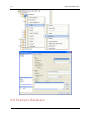
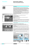
6.6 Create a new Database
It is quite simple to create a new database in Microsoft SQL Server. Just right-click on the
“Databases” node and select “New Database…”
Tutorial: Database Communication in LabVIEW
23
Microsoft SQL Server
There are lots of settings you may set regarding your database, but the only information you must fill
in is the name of your database:
Tutorial: Database Communication in LabVIEW
24
Microsoft SQL Server
6.7 Backup/Restore
An important task in database systems is to take backup of the database with regular intervals, e.g.,
during the night when the system is not in use.
Database backup and Restore:
Tutorial: Database Communication in LabVIEW
25
Microsoft SQL Server
6.8 Example Database
Tutorial: Database Communication in LabVIEW
26
Microsoft SQL Server
Examples and exercises in this training are based on some basic tables. The Example Database
consists of the following Tables:




CUSTOMER
o CustomerId (PK)
o FirstName
o LastName
o Address
o Phone
o PostCode
o PostAddress
PRODUCT
o ProductId (PK)
o ProductName
o ProductDescription
o Price
o ProductCode
ORDER
o OrderId (PK)
o OrderNumber
o OrderDescription
o CustomerId (FK)
ORDER_DETAIL
o OrderDetailId (PK)
o OrderId (FK)
o ProductId (FK)
Tutorial: Database Communication in LabVIEW
27
Microsoft SQL Server
6.9 Exercises
Exercise: New Database
Create a new Database in MS SQL Server called TEST_SQLSERVER.
Exercise: Database Diagram
Create the tables in the Example Database using the Diagram Designer Tool in Microsoft SQL Server.
Exercise: Database Script
Create the tables in the Example Database Tables using SQL Code. Save the Tables as a SQL Script file
(.sql). Use The Query Tool in Microsoft SQL Server.
Exercise: ODBC
Create an ODBC connection for the Database.
Tutorial: Database Communication in LabVIEW
7 Microsoft Office Access
7.1 Introduction
Microsoft Office Access, previously known as Microsoft Access, is a relational database management
system from Microsoft that combines the relational Microsoft Jet Database Engine with a graphical
user interface and software development tools. It is a member of the Microsoft Office suite of
applications and is included in the Professional and higher versions for Windows. Access stores data
in its own format based on the Access Jet Database Engine.
Microsoft Access is used by programmers and non-programmers to create their own simple database
solutions.
Microsoft Access is a file server-based database. Unlike client-server relational database
management systems (RDBMS), e.g., Microsoft SQL Server, Microsoft Access does not implement
database triggers, stored procedures, or transaction logging. All database tables, queries, forms,
reports, macros, and modules are stored in the Access Jet database as a single file. This makes
Microsoft Access useful in small applications, teaching, etc. because it is easy to move from one
computer to another.
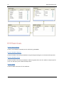
7.2 Example Database
I will present an example database in Microsoft Access 2007 which will be used in some of the
examples and exercises in this document.
The database consists of the following tables:


CUSTOMER
o CustomerId (PK)
o FirstName
o LastName
o Address
o Phone
o PostCode
o PostAddress
PRODUCT
o ProductId (PK)
o ProductName
28
29
Microsoft Office Access


o ProductDescription
o Price
o ProductCode
ORDER
o OrderId (PK)
o OrderNumber
o OrderDescription
o CustomerId (FK)
ORDER_DETAIL
o OrderDetailId (PK)
o OrderId (FK)
o ProductId (FK)
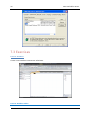
ODBC Connection:
Administrative Tools → Data Sources (ODBC)
Tutorial: Database Communication in LabVIEW
30
Microsoft Office Access
7.3 Exercises
Exercise: Database
Create a new Database in MS Access called TEST.
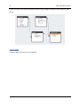
Exercise: Database Tables
Tutorial: Database Communication in LabVIEW
31
Microsoft Office Access
Create the tables in the Example Database Tables using the Diagram Designer Tool in Microsoft SQL
Server.
Exercise: ODBC
Create an ODBC connection for the Database.
Tutorial: Database Communication in LabVIEW
8 ODBC
8.1 What is ODBC?
In computing, Open Database Connectivity (ODBC) provides a standard software API method for
using database management systems (DBMS). The designers of ODBC aimed to make it independent
of programming languages, database systems, and operating systems.
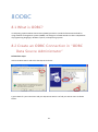
8.2 Create an ODBC Connection in “ODBC
Data Source Administrator”
Follow these steps:
Add a new Data Source and select the SQL Server driver:
Type a Name for your Connection and your SQL Server Name. You find your Server name as shown
below:
32
33
ODBC
Select SQL Server authentication and type your sa password (System Administrator).
the password for the sa user during the setup procedure of SQL Server:
Complete your configuration and Test your data source to see if its OK:
Tutorial: Database Communication in LabVIEW
You defined
34
ODBC
If you get this message you have succeeded:
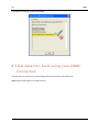
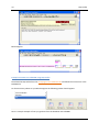
8.3 Get data into Excel using your ODBC
Connection
The purpose is to use Excel as a client and get data into Excel from your SQL Server.
Step 1: Open Excel and go to the Data section:
Tutorial: Database Communication in LabVIEW
35
ODBC
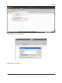
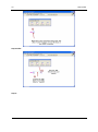
Step 2: Select your ODBC connection
Step 3: Select your Table(s)
Tutorial: Database Communication in LabVIEW
36
ODBC
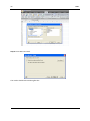
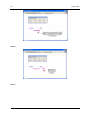
Step 4: Insert Data into Excel
The results should look something like this:
Tutorial: Database Communication in LabVIEW
37
ODBC
Tutorial: Database Communication in LabVIEW
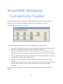
9 LabVIEW Database
Connectivity Toolkit
LabVIEW offers an additional Toolkit called “LabVIEW Database Connectivity Toolkit”. With this
toolkit you can communicate with different databases, such as SQL Server, Oracle, etc.
Functions Palette: Connectivity → Database
The following list describes the main features of the Database Connectivity Toolkit:







Works with any provider that adheres to the Microsoft ActiveX Data Object (ADO) standard.
Works with any database driver that complies with ODBC or OLE DB.
Maintains a high level of portability. In many cases, you can port an application to another
database by changing the connection information you pass to the DB Tools Open Connection
VI.
Converts database column values from native data types to standard Database Connectivity
Toolkit data types, further enhancing portability.
Permits the use of SQL statements with all supported database systems, even non-SQL
systems.
Includes VIs to retrieve the name and data type of a column returned by a SELECT statement.
Creates tables and selects, inserts, updates, and deletes records without using SQL
statements.
Some of the text in this chapter is based on the “LabVIEW Database Connectivity Toolkit User
Manual”.
38
39
LabVIEW Database Connectivity Toolkit
9.1 Connect to the Database
Before you can access data in a table or execute SQL statements, you must establish a connection to
a database. You may use different methods in order to connect to the database:



ODBC Data Source Name (DSN)
Universal Data Link (UDL)
Connection String
These different methods are explained below.
For all of these methods, you will use the same VI:
Connecting to a database is where most errors occur because each database management system
(DBMS) uses different parameters for the connection and different levels of security. The different
standards also use different methods of connecting to databases. For example, ODBC uses Data
Source Names (DSN) for the connection, whereas the Microsoft ActiveX Data Object (ADO) standard
uses Universal Data Links (UDL) for the connection. The “DB Tools Open Connection.vi” VI supports
all these methods for connecting to a database.
When you are finished with reading from the database and writing to the database, you should
always close the Connection. Use the “DB Tools Close Connection.vi”.
Tutorial: Database Communication in LabVIEW
40
9.1.1
LabVIEW Database Connectivity Toolkit
DSN
A DSN (ODBC Data Source Name (DSN)) is the name of the data source, or database, to which you
are connecting. The DSN also contains information about the ODBC driver and other connection
attributes including paths, security information, and read-only status of the database. Two main
types of DSNs exist: machine DSNs and file DSNs. Machine DSNs are in the system registry and apply
to all users of the computer system or to a single user. DSNs that apply to all users of a computer
system are system DSNs. DSNs that apply to single users are user DSNs. A file DSN is a text file with a
.dsn extension and is accessible to anyone with proper permissions. File DSNs are not restricted to a
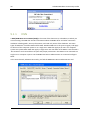
single user or computer system. Use the ODBC Data Source Administrator to create and configure
DSNs.
In the Control Panel, Administrative Tools, you find the ODBC Data Source Administrator tool.
Tutorial: Database Communication in LabVIEW
41
LabVIEW Database Connectivity Toolkit
Example: DSN
This Example specifies a DSN called MS Access to open a connection to that specific database.
Example: DSN from File
You can use a path to specify a file DSN. This example specifies a path to a file DSN called
“access.dsn” to open a connection to the database.
Example: DSN with UserId and Password
Most Database systems (DBMS – Database Management Systems) also require a UserId and a
Password.
9.1.2
UDL
Whereas you must create a DSN to connect to a database using ODBC, you use UDL (Universal Data
Link) to connect to databases that use ADO and OLE DB.
A UDL is similar to a DSN in that it describes more than just the data source. A UDL specifies what
OLE DB provider is used, server information, the user ID and password, the default database, and
other related information.
In order to create a new UDL file, create an empty text file and change the file extension of this
document from .txt to .udl. You then can double-click the UDL file to display the Data Link Properties
dialog box.
Tutorial: Database Communication in LabVIEW
42
LabVIEW Database Connectivity Toolkit
Example: UDL
Connect to a Database using UDL:
9.1.3
Connection String
Rather than including an existing UDL in an application, you also can use an ODBC connection string
with the Microsoft ActiveX Data Object (ADO) standard.
A connection string is written like this:
PROVIDER=SQLOLEDB;DATA
SOURCE=server_name;UID=user_name;PWD=password;DATABASE=database_name;
You could use more parameters, but the parameters used above are the most common ones.
9.2 Reading Data from the Database
Reading data from a database table is similar to writing data to the database. You open a connection
to the database, select the data from a table, and then close the connection.
Tutorial: Database Communication in LabVIEW
43
LabVIEW Database Connectivity Toolkit
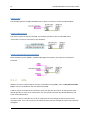
The “DB Tools Select Data.vi" is used to read data from the Database:
Example: Select Data from MS Access
The following example gets data from the CUSTOMER table in MS Access.
The Front Panel looks like this:
Notice in Figures 5-4 and 5-5 that the database data is returned as a two-dimensional array of
variants. As the name implies, the Microsoft ActiveX Data Object (ADO) standard is based on ActiveX,
which defines variants as its data types. Variants work well in languages such as Visual Basic that are
not strongly typed. Because LabVIEW is strongly typed, you must use the Database Variant To Data
Tutorial: Database Communication in LabVIEW
44
LabVIEW Database Connectivity Toolkit
function to convert the variant data to a LabVIEW data type before you can display the data in
standard indicators such as graphs, charts, and LEDs.
Example: Select Data from MS Access
The following example gets data from the CUSTOMER table in MS Access and converts the data to
text.
The Front Panel looks like this:
You may read from more than one table if you use a comma-delimited string to specify multiple table
names:
Tutorial: Database Communication in LabVIEW
45
LabVIEW Database Connectivity Toolkit
You may select which columns you want to read by using the “Columns” input:
You may also restrict which data to receive using the “optional Clause” input:
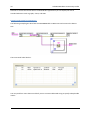
Example: Read Data
Using some VIs from the “Advanced” palette, create the following example:
Tutorial: Database Communication in LabVIEW
46
LabVIEW Database Connectivity Toolkit
9.3 Writing Data to the Database
Writing data to a database with the LabVIEW Database Connectivity Toolkit is similar to reading data
to a file. You open a connection, insert the data, and close the connection when you are finished.
The “DB Tools Insert Data.vi" is used to write data to the Database:
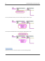
Example: Write Data
Create the following block diagram:
Tutorial: Database Communication in LabVIEW
47
LabVIEW Database Connectivity Toolkit
Front Panel:
Example: Write Data
Create the following block diagram using some VIs from the “Advanced” palette.
Tutorial: Database Communication in LabVIEW
48
LabVIEW Database Connectivity Toolkit
9.4 Creating and Dropping Tables
You may use standard SQL syntax in order to create:
CREATE TABLE <TableName> (…)
Or you may use the “DB Tools Create Table.vi” in order to create a table.
You may use standard SQL syntax in order to drop tables (delete tables):
DROP TABLE <TableName>
Or you may use the “DB Tools Drop Table.vi” in order to drop/delete a table.
Tutorial: Database Communication in LabVIEW
49
LabVIEW Database Connectivity Toolkit
9.5 Using the Database Connectivity Toolkit
Utility VIs
In the “Utility” palette there are several useful VIs for getting more information about tables, saving
to text files, etc.
Here is a short description of the VIs located in the “Utility” palette:
This VI lists the tables in the database identified by connection reference.
This VI lists the columns present in table. The column information includes the
name, the data type, and the defined size of the column.
This VI sets properties on the object as determined by the inputs.
This VI gets properties of the object as determined by the inputs.
This VI Returns a string containing the formatted date and time, and
identifies the string as a date/time string so other VIs can interpret it.
This VI begins, commits, or rolls back a transaction for any type of
reference.
Tutorial: Database Communication in LabVIEW
50
LabVIEW Database Connectivity Toolkit
This VI saves the recordset identified by the recordset reference to
either an XML or ADTG file. The ADTG file format is a proprietary format that only the LabVIEW
Database Connectivity Toolkit can interpret. The ADTG format results in a smaller file than the XML
format.
This VI loads a recordset from a file and returns a recordset
reference that identifies this recordset. You can retrieve data from this recordset like any other
recordset, but some properties might not be available on this recordset.
9.6 Performing Advanced Database
Operations
When creating real programs you will soon need some of the VIs in the “Advanced” palette.
Here is a short description of some of the VIs located in the “Advanced” palette:
This VI Executes an SQL query and returns a recordset reference that you
must eventually free with the DB Tools Free Object VI.
This VI retrieves the data in the recordset identified by the recordset
reference input. You can convert each element in the array to its native LabVIEW data type using the
“Database Variant To Data function”.
Tutorial: Database Communication in LabVIEW
51
LabVIEW Database Connectivity Toolkit
This VI frees an object by destroying its associated reference and returns a
different reference object.
Tutorial: Database Communication in LabVIEW
10 Creating and Using
Tables
The SQL syntax for creating a Table is as follows:
CREATE TABLE <TableName>
(
<ColumnName> <datatype>
…
)
The SQL syntax for inserting Data into a Table is as follows:
INSERT INTO <TableName> (<Column1>, <Column2>, …)
VALUES(<Data for Column1>, <Data for Column2>, …)
Example: Insert Data into Tables
We will insert some data into our tables:
52
53
Creating and Using Tables
The following SQL Query inserts some example data into these tables:
--CUSTOMER
INSERT INTO [CUSTOMER]
([FirstName],[LastName],[Address],[Phone],[PostCode],[PostAddress]) VALUES
('Per', 'Nilsen', 'Vipeveien 12', '12345678', '1234', 'Porsgrunn')
GO
INSERT INTO [CUSTOMER]
([FirstName],[LastName],[Address],[Phone],[PostCode],[PostAddress]) VALUES
('Tor', 'Hansen', 'Vipeveien 15', '77775678', '4455', 'Bergen')
GO
INSERT INTO [CUSTOMER]
([FirstName],[LastName],[Address],[Phone],[PostCode],[PostAddress]) VALUES
('Arne', 'Nilsen', 'Vipeveien 17', '12345778', '4434', 'Porsgrunn')
GO
--PRODUCT
INSERT INTO [PRODUCT]
([ProductName],[ProductDescription],[Price],[ProductCode]) VALUES ('Product
A', 'This is product A', 1000, 'A-1234')
GO
INSERT INTO [PRODUCT]
([ProductName],[ProductDescription],[Price],[ProductCode]) VALUES ('Product
B', 'This is product B', 1000, 'B-1234')
GO
INSERT INTO [PRODUCT]
([ProductName],[ProductDescription],[Price],[ProductCode]) VALUES ('Product
C', 'This is product C', 1000, 'C-1234')
GO
--ORDER
INSERT INTO [ORDER] ([OrderNumber],[OrderDescription],[CustomerId]) VALUES
('10001', 'This is Order 10001', 1)
GO
INSERT INTO [ORDER] ([OrderNumber],[OrderDescription],[CustomerId]) VALUES
('10002', 'This is Order 10002', 2)
GO
INSERT INTO [ORDER] ([OrderNumber],[OrderDescription],[CustomerId]) VALUES
('10003', 'This is Order 10003', 3)
GO
--ORDER_DETAIL
INSERT INTO [ORDER_DETAIL]
GO
INSERT INTO [ORDER_DETAIL]
GO
INSERT INTO [ORDER_DETAIL]
GO
INSERT INTO [ORDER_DETAIL]
GO
INSERT INTO [ORDER_DETAIL]
GO
INSERT INTO [ORDER_DETAIL]
GO
INSERT INTO [ORDER_DETAIL]
GO
INSERT INTO [ORDER_DETAIL]
GO
([OrderId],[ProductId]) VALUES (1, 1)
([OrderId],[ProductId]) VALUES (1, 2)
([OrderId],[ProductId]) VALUES (1, 3)
([OrderId],[ProductId]) VALUES (2, 1)
([OrderId],[ProductId]) VALUES (2, 2)
([OrderId],[ProductId]) VALUES (3, 3)
([OrderId],[ProductId]) VALUES (3, 1)
([OrderId],[ProductId]) VALUES (3, 2)
Tutorial: Database Communication in LabVIEW
54
Creating and Using Tables
INSERT INTO [ORDER_DETAIL] ([OrderId],[ProductId]) VALUES (3, 3)
GO
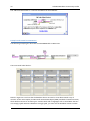
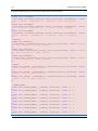
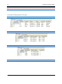
Executing the following Queries then gives:
select * from CUSTOMER
select * from PRODUCT
select * from [ORDER]
select * from ORDER_DETAIL
Tutorial: Database Communication in LabVIEW
55
10.1
Creating and Using Tables
Exercises
Run the queries above from LabVIEW.
Tutorial: Database Communication in LabVIEW
11 Creating and Using
Views
In database theory, a view consists of a stored query accessible as a virtual table composed of the
result set of a query. Unlike ordinary tables in a relational database, a view does not form part of the
physical schema: it is a dynamic, virtual table computed or collated from data in the database.
Changing the data in a table alters the data shown in subsequent invocations of the view.
Views can provide advantages over tables:







Views can represent a subset of the data contained in a table
Views can join and simplify multiple tables into a single virtual table
Views can act as aggregated tables, where the database engine aggregates data (sum,
average etc) and presents the calculated results as part of the data
Views can hide the complexity of data; for example a view could appear as Sales2000 or
Sales2001, transparently partitioning the actual underlying table
Views take very little space to store; the database contains only the definition of a view, not
a copy of all the data it presents
Depending on the SQL engine used, views can provide extra security
Views can limit the degree of exposure of a table or tables to the outer world
Just as functions (in programming) can provide abstraction, so database users can create abstraction
by using views. In another parallel with functions, database users can manipulate nested views, thus
one view can aggregate data from other views.
Syntax:
CREATE VIEW <ViewName>
AS
…
Create a VIEW:
Step 1: Create a new View
56
57
Creating and Using Tables
Step 2: Add your tables
Step 3: Add your columns
Tutorial: Database Communication in LabVIEW
58
Creating and Using Tables
Step 4: Save it
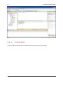
Using the VIEW in a Query:
Tutorial: Database Communication in LabVIEW
59
11.1
Creating and Using Tables
Exercises
Create a simple view based on the example tables and run the view from LabVIEW.
Tutorial: Database Communication in LabVIEW
12 Creating and using
Stored Procedures
A stored procedure is a subroutine available to applications accessing a relational database system.
Typical uses for stored procedures include data validation (integrated into the database) or access
control mechanisms. Furthermore, stored procedures are used to consolidate and centralize logic
that was originally implemented in applications. Large or complex processing that might require the
execution of several SQL statements is moved into stored procedures, and all applications call the
procedures only.
A stored procedure is a precompiled collection of SQL statements and optional control-of-flow
statements, similar to a macro. Each database and data provider supports stored procedures
differently. Stored procedures offer the following benefits to your database applications:
Performance—Stored Procedures are usually more efficient and faster than regular SQL queries
because SQL statements are parsed for syntactical accuracy and precompiled by the DBMS when the
stored procedure is created. Also, combining a large number of SQL statements with conditional logic
and parameters into a stored procedure allows the procedures to perform queries, make decisions,
and return results without extra trips to the database server.
Maintainability—Stored Procedures isolate the lower-level database structure from the application.
As long as the table names, column names, parameter names, and types do not change from what is
stated in the stored procedure, you do not need to modify the procedure when changes are made to
the database schema. Stored procedures are also a way to support modular SQL programming
because after you create a procedure, you and other users can reuse that procedure without
knowing the details of the tables involved.
Security—When creating tables in a database, the Database Administrator can set EXECUTE
permissions on stored procedures without granting SELECT, INSERT, UPDATE, and DELETE
permissions to users. Therefore, the data in these tables is protected from users who are not using
the stored procedures.
Stored procedures are similar to user-defined functions. The major difference is that functions can be
used like any other expression within SQL statements, whereas stored procedures must be invoked
using the CALL statement.
The syntax for creating a Stored Procedure is as follows:
CREATE PROCEDURE <ProcedureName>
@<Parameter1> <datatype>
60
61
Creating and using Stored Procedures
…
Example: Create a Stored Procedure
This Procedure gets Customer Data based on a specific Order Number.
IF EXISTS (SELECT name
FROM
sysobjects
WHERE name = 'sp_CustomerOrders'
AND
type = 'P')
DROP PROCEDURE sp_CustomerOrders
GO
CREATE PROCEDURE sp_CustomerOrders
@OrderNumber varchar(50)
AS
/*------------------------------------------------------------------------Last Updated Date:
2009.11.03
Last Updated By:
[email protected]
Description:
Get Customer Information from a specific Order Number
-------------------------------------------------------------------------*/
SET NOCOUNT ON
declare @CustomerId int
select @CustomerId = CustomerId from [ORDER] where OrderNumber = @OrderNumber
select CustomerId, FirstName, LastName, [Address], Phone from CUSTOMER where
CustomerId=@CustomerId
SET NOCOUNT OFF
GO
Example: Using a Stored Procedure
Using the Stored procedure like this
exec sp_CustomerOrders '10002'
gives the following result:
Tutorial: Database Communication in LabVIEW
62
12.1
Creating and using Stored Procedures
Exercises
Run the Stored Procedure created above from LabVIEW.
Tutorial: Database Communication in LabVIEW
13 Creating and Using
Triggers
A database trigger is procedural code that is automatically executed in response to certain events on
a particular table or view in a database. The trigger is mostly used for keeping the integrity of the
information on the database. For example, when a new record (representing a new worker) added to
the employees table, new records should be created also in the tables of the taxes, vacations, and
salaries.
Triggers are commonly used to:








prevent changes (e.g. prevent an invoice from being changed after it's been mailed out)
log changes (e.g. keep a copy of the old data)
audit changes (e.g. keep a log of the users and roles involved in changes)
enhance changes (e.g. ensure that every change to a record is time-stamped by the server's
clock, not the client's)
enforce business rules (e.g. require that every invoice have at least one line item)
execute business rules (e.g. notify a manager every time an employee's bank account
number changes)
replicate data (e.g. store a record of every change, to be shipped to another database later)
enhance performance (e.g. update the account balance after every detail transaction, for
faster queries)
The major features of database triggers, and their effects, are:




do not accept parameters or arguments (but may store affected-data in temporary tables)
cannot perform commit or rollback operations because they are part of the triggering SQL
statement
can cancel a requested operation
can cause mutating table errors, if they are poorly written.
Microsoft SQL Server supports triggers either after or instead of an insert, update, or delete
operation.
The syntax is as follows:
63
64
Creating and using Stored Procedures
CREATE TRIGGER <TriggerName>
FOR INSERT, UPDATE, DELETE
AS
… Create your Code here
GO


on <TableName>
Replace <TriggerName> with the Name of your Trigger
Replace <TableName> with the Name of your Table
Define when the Trigger should be execute





If the Trigger should be executed only when you insert data into the table: FOR INSERT
If the Trigger should be executed only when you update data into the table: FOR UPDATE
If the Trigger should be executed only when you delete data into the table: FOR DELETE
If the Trigger should be executed when you insert and update data into the table: FOR
INSERT, UPDATE
Etc.
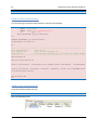
Example: Trigger
The Example above change the “below” in the Table “SCHOOL” from ‘TUC’ to ‘Telemark University
College’
CREATE TRIGGER CheckSchoolData on SCHOOL
FOR INSERT, UPDATE
AS
DECLARE
@SchoolName varchar(50)
select @SchoolName=SchoolName from INSERTED
If @SchoolName='TUC'
update SCHOOL set SchoolName='Telemark University College' where
SchoolName=@SchoolName
GO
Note! Note the use of a temporary table called “INSERTED”. This temporary table contains the last
inserted record into the SCHOOL table
Note! In SQL you define a variable like this
DECLARE
@myVariable <datatype>
Example:
DECLARE
@SchoolName varchar(10)
Tutorial: Database Communication in LabVIEW
65
Creating and using Stored Procedures
Note! You have to use the symbol “@” before the name of the variable!!!
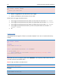
Below we see how we create a Trigger from the “SQL Server Management Studio”:
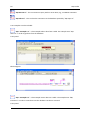
Check if the Trigger is working as expected:
Procedure:
Step 1: Check the data in your table before you do anything, e.g.:
select * from SCHOOL
Step 2: Insert some test data into your table, e.g.:
insert into SCHOOL (SchoolId, SchoolName) values (5, 'TUC')
Step 3: Check the data has been updated according to your code in the Trigger:
select * from SCHOOL
Tutorial: Database Communication in LabVIEW
66
Creating and using Stored Procedures
→ As you see the data you inserted into the table has been automatically been changed by the
Trigger
13.1
Exercises
Create a Trigger that adds “+47” to all Phone numbers in the CUSTOMER table.
Test and see if the Trigger works properly by inserting and updating some data in the CUSTOMER
table.
Tutorial: Database Communication in LabVIEW
14 Creating and using
Functions
In SQL databases, a user-defined function provides a mechanism for extending the functionality of
the database server by adding a function that can be evaluated in SQL statements. The SQL standard
distinguishes between scalar and table functions. A scalar function returns only a single value (or
NULL), whereas a table function returns a (relational) table comprising zero or more rows, each row
with one or more columns.
Stored Procedures vs. Functions:







Only functions can return a value (using the RETURN keyword).
Stored procedures can use RETURN keyword but without any value being passed[1]
Functions could be used in SELECT statements, provided they don’t do any data manipulation
and also should not have any OUT or IN OUT parameters.
Functions must return a value, but for stored procedures this is not compulsory.
A function can have only IN parameters, while stored procedures may have OUT or IN OUT
parameters.
A function is a subprogram written to perform certain computations and return a single
value.
A stored procedure is a subprogram written to perform a set of actions, and can return
multiple values using the OUT parameter or return no value at all.
User-defined functions in SQL are declared using the CREATE FUNCTION statement.
14.1
Exercises
Create a simple function that finds number of order for a specific customer and use it in the following
query:
“Select FirstName, LastName, fn_NumberOfOrders(CustomerId) from CUSTOMER”
67
15 SQL Toolkit
I have made a simple and easy to-use SQL Toolkit. The SQL Toolkit is available for download from my
Blog: http://home.hit.no/~hansha/
15.1
Installation
The installation procedure is as follows:
1.
2.
3.
4.
5.
Download the zip file SQLToolkit.zip from my Blog
Unzip the file
Copy "SQLToolkit.mnu" to ...\LabVIEW 2009\menus\Categories\
Copy "SQLToolkit.llb" to ...\LabVIEW 2009\vi.lib\
The SQL Toolkit is ready to use and in the Functions palette in LabVIEW a new palette named
"SQL" will appear.
The SQL Toolkit palette in available in LabVIEW:
The SQL Toolkit contains the following VIs:
“SQL Open.vi” - This VI open a connection to the database specified in the Connection string.
The connection string may be as follows:
“PROVIDER=SQLOLEDB; DATA SOURCE=xxx;UID=xxx;PWD=xxx;DATABASE=xxx”
You need to replace the “xxx” with the parameters from your database.
“SQL Select.vi” -This VI get data from the database specified in the SQL Query. The output is a
2D string array with data.
68
69
SQL Toolkit
“SQL Execute.vi” - This VI executes a Query with no return Data, e.g., an INSERT statement
“SQL Close.vi” - This VI Close the connection to the database opened by "SQL Open.vi"
Two examples are also included:
“SQL – Example 1.vi” – This example selects data from a table. The example uses “SQL
Select.vi” in order to get data from the database.
Front panel:
Block Diagram:
“SQL – Example 2.vi” – This example inserts data into a table. The example uses “SQL
Execute.vi” in order to insert data into the database. No data is returned.
Front panel:
Tutorial: Database Communication in LabVIEW
70
SQL Toolkit
Block Diagram:
Example: Get Data into LabVIEW using SQL Toolkit
Download the SQL toolkit from the Homepage of the Database Lab and follow the instructions in the
ReadMe file.
On the Functions palette on your Block Diagram the following palette should appear:
Here is a simple example of how you get data from the database into LabVIEW:
Tutorial: Database Communication in LabVIEW
71
SQL Toolkit
The procedure is as follows:
Step 1:
Step 2:
Tutorial: Database Communication in LabVIEW
72
SQL Toolkit
Step 3 and 4:
Step 5:
Tutorial: Database Communication in LabVIEW
73
SQL Toolkit
Step 6:
Step 7:
Tutorial: Database Communication in LabVIEW
74
SQL Toolkit
Step 8:
Tutorial: Database Communication in LabVIEW
Telemark University College
Faculty of Technology
Kjølnes Ring 56
N-3914 Porsgrunn, Norway
www.hit.no
Hans-Petter Halvorsen, M.Sc.
Telemark University College
Department of Electrical Engineering, Information Technology and Cybernetics
Phone: +47 3557 5158
E-mail: [email protected]
Blog: http://home.hit.no/~hansha/
Room: B-237a